A New Method to Analyze the Tsunami Incitement Process …tsunamisociety.org/282Zhub.pdf · 1 A New Method to Analyze the Tsunami Incitement Process and Site-selection for Tsunami

1

A New Method to Analyze the Tsunami Incitement Process and Site-selection for

Tsunami Observations in China's Eastern Sea

Yuanqing Zhu1,

Shuangqing Liu,

Yanlin Wen,

Yan Xue 1Professor, Earthquake Administration of Shanghai Municipality;

National Geophysical Observatory at Sheshan, Shanghai, 200062, China

Email: [email protected], [email protected]

ABSTRACT

In this paper, we present a CONTROL volume model for tsunami incitement process by combining the

Navier-Stokes equation, the jet theory and relative velocity model. We conclude that the initial condition for

tsunami propagation simulation is equivalent to the static near-field seismic displacement of earthquake that

induces the tsunami. The error analyzed from this method is only about 1 percent for a common seafloor

earthquake, and it is consistent with the result of Ansys/Ls-dyna numerical analysis. EDGRN/EDCMP and

COMCOT program provide some new acquirement for the tsunami studies. In the second part of the paper, we

develop a site-selection method for anchor-grounded tsunami observation in Chinese eastern sea.

KEYWORDS: N-S equation, Jet theory, Relative velocity, Optimal analysis

INTRODUCTION

At present, there is little solid and constructive study on the tsunami near-field characteristics or initial

condition of propagating simulation. The classic paper by Gutenberg (1939) showed that most previous studies

on tsunami were rested on the qualitative approaches. The essential study about the tsunami near-field

characteristics maybe owned to Kajiura (1970). He separated the energy pattern from the non-homogeneous

wave equation. Most of subsequent tsunami propagation researches all made a statement to cite its conclusion,

albeit there was a defect in that article, which the energy of dynamic retrieved from the incitement source was

completely independent of the water depth. Based on the linear shallow water wave equations, Todorovska et al.

(2001,2002,2003) derived analytical integral solution for tsunami incited by a landslide. Ward (2003) deduced,

with traditional seismological procedures, some 1st-order approximate integral formula of results including

patterns of incitement of the landslide, celestial impact, and seismic tensor combined with focal geometry

parameters. Ohmachi et al. (2001) utilized BEM and FDM methods to simulate a tsunami incitement process by

a fault rupture. Partial interrelated experiments and corresponding numerical calculations were carried out by

Grilli et al. (2001,2004,2005) and Liu et al. (2005). Except above, most researches put focus on the propagation

and simulation algorithm, and paid little attention to the “initial value problem.” We present a new way to

analyze the tsunami near-field characteristics. Also, in the part 2, we discuss the method for selecting a best site

for anchor-grounded tsunami observational station.

Science of Tsunami Hazards, Vol. 28, No. 2, page 129 (2009)

2

PART (I) INITIAL VALUE PROBLEM

Mathematical Model

In general fluid mechanism theory, the Navier-Stokes momentum equation is

)(1

jiijTt

eefVVV

!"+="!+#

#

$ (1)

Where, V is velocity vector, f is body force, ! is density, Tij is a tenor, and ei, ej is unit directional vector. This is a

differential equation. Along with the continuous equation: 0)( =!"+#

#V$

$

t

, it constitutes the traditional

foundation of fluid mechanism theory. Especially, they are suitable for the shallow wave studies. However, these

equations only allow researchers to derive the complex integral solutions to the wave initial deformation, it is still

difficult to obtain the relationship between the tsunami and its incitement source, even for the case in which the

hypothesis source is very simple. But if we consider the integral equation form of momentum is

! !! ! !!" "

+=#+$

$D D

ndAddAd

tTfnVV

VV)(V

)(%%

% (2)

Where n is a normal vector. We can develop a CONTROL volume model to analyze it.

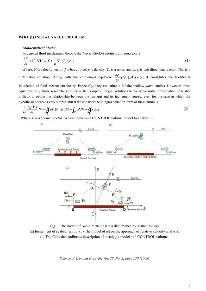
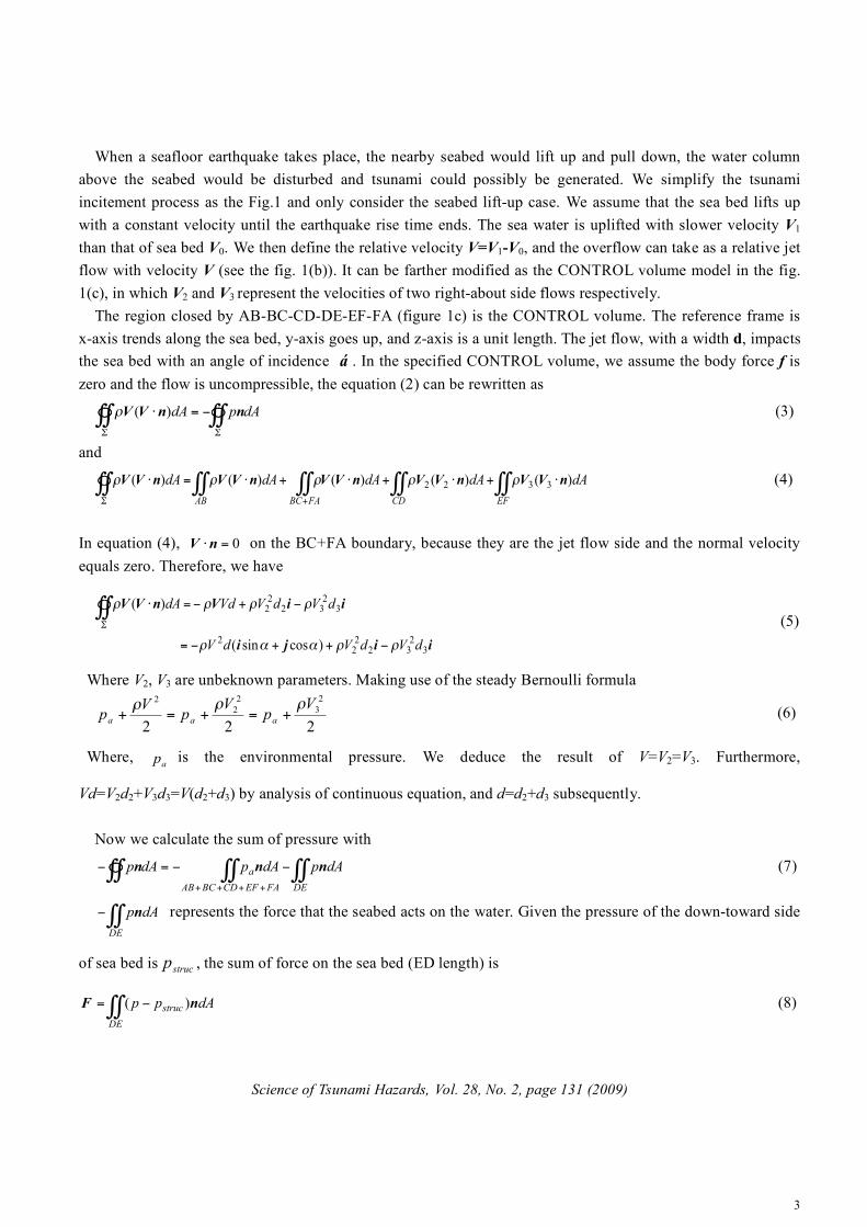
Fig .1 The sketch of two-dimensional sea disturbance by seabed run-up

(a) Incitement of seabed run up, (b) The model of jet on the approach of relative velocity analysis,

(c) The Cartesian-ordinates description of steady jet model and CONTROL volume.


3

When a seafloor earthquake takes place, the nearby seabed would lift up and pull down, the water column

above the seabed would be disturbed and tsunami could possibly be generated. We simplify the tsunami

incitement process as the Fig.1 and only consider the seabed lift-up case. We assume that the sea bed lifts up

with a constant velocity until the earthquake rise time ends. The sea water is uplifted with slower velocity V1

than that of sea bed V0. We then define the relative velocity V=V1-V0, and the overflow can take as a relative jet

flow with velocity V (see the fig. 1(b)). It can be farther modified as the CONTROL volume model in the fig.

1(c), in which V2 and V3 represent the velocities of two right-about side flows respectively.

The region closed by AB-BC-CD-DE-EF-FA (figure 1c) is the CONTROL volume. The reference frame is

x-axis trends along the sea bed, y-axis goes up, and z-axis is a unit length. The jet flow, with a width d, impacts

the sea bed with an angle of incidence á . In the specified CONTROL volume, we assume the body force f is

zero and the flow is uncompressible, the equation (2) can be rewritten as

dApdA !!!!""

#=$ nnVV )(% (3)

and

dAdAdAdAdA

EFCDAB FABC

)()()()()( 3322 nVVnVVnVVnVVnVV !+!+!+!=! """""" "" ""# +

$$$$$ (4)

In equation (4), 0=!nV on the BC+FA boundary, because they are the jet flow side and the normal velocity

equals zero. Therefore, we have

iiji

iiVnVV

3232

22

2

3232

22

)cossin(

)(

dVdVdV

dVdVVddA

!!""!

!!!!

#++#=

#+#=$%%& (5)

Where V2, V3 are unbeknown parameters. Making use of the steady Bernoulli formula

222

2

3

2

2

2 Vp

Vp

Vp aaa

!!!+=+=+ (6)

Where, ap is the environmental pressure. We deduce the result of V=V2=V3. Furthermore,

Vd=V2d2+V3d3=V(d2+d3) by analysis of continuous equation, and d=d2+d3 subsequently.

Now we calculate the sum of pressure with

!!!!!! ""="

++++ DEFAEFCDBCAB

a dApdApdAp nnn (7)

!!"

DE

dApn represents the force that the seabed acts on the water. Given the pressure of the down-toward side

of sea bed isstrucp , the sum of force on the sea bed (ED length) is

!! "=

DE

struc dApp nF )( (8)


4

Substitute p into equation (7), we have

!!!!!!!!

!!!!!!!!!!!!

+""=

"+""="=

++++

DE

a

DE

struca

DE

a

DE

a

DE

struc

FAEFCDBCAB

a

DE

struc

dApdApdApdAp

dApdApdApdApdApdApp

nnnn

nnnnnnF )(

(9)

The second item on the right is equal to zero as it integrates on a closed facet. And equation (9) can be

simplified as

!!!!!! +"=

DE

a

DE

struc dApdApdAp nnnF (10)

Substitute equations (10), (5) into (3):

!!!! +""="++"

DE

a

DE

struc dApdApdVdVdV nnFiiji 32

222 )cossin( ##$$#

then

ijnn

nniijiF

)sin()cos(

)cossin(

23

22

22

32

222

!"""!"

""!!"

dVdVdVdVdApdAp

dApdApdVdVdV

DE

a

DE

struc

DE

a

DE

struc

###++#=

+#+#+=

$$$$

$$$$ (11)

Considering the water is approximately an idealized fluid, only the normal force exists on the seabed, and the

x-axis component of F is zero.

jnnF )cos( 2 !" dVdApdAp

DE

a

DE

struc ++#= $$$$ (12)

!sin32ddd =" (13)

Since ddd =+32

, we have 2

)sin1(2

!+=d

d and2

)sin1(3

!"=d

d .

Hereby, the inter-force on the interface between water and sea bed can be written as

!!""=

DE

aeraction dApdV njF )cos( 2int #$ (14)

Therefore, Finteraction is a function of the fluid density, relative velocity and incidence angle of jet, the pressure

of environment, and the ED length of seabed incitement. If we assume the length of ED is l, ld != , !" (0,1)

is a ratio (we define it as a factor of effective width of jet flow), then

njF !""# ghllVeraction $%&$ )cos( 2int

)cos(cos|||| 221int ghVlghllVF eraction +=+= !"##!"# (15)

In fact, the value of ! reflects the homogenization of fluid velocity and pressure on the entrance and exit of

jet. Where, g is the gravity acceleration force, h is the depth of water.


5

We can also consider the effect of Finteraction to the water energy by the formula !!"

#=$

$dA

t

EnVT , where E is

the total energy of water.

!!

!!!!!!

"

"""

+=

##$$=#=#=%

%

dAghVVl

dAghllVdAdAt

Eeractionn

)coscos(

))cos((

22

2

int

&&'(

(&'( VnjVFVT

(16)

The above equation is very simple but with an important implication to separate the pattern of energy. We can

define Q to illustrate the result as well:

ghVcQ /2

!= (17)

Where, c is the ratio of !" 2cos and !cos in the equation (16).

It is believed that, once a tsunami is induced by an earthquake, the uplift velocity of seabed is between

0.1-10m/s, and h is between 500-5000m. According to Equation (17), Q would be in the range of 2.04!10-7

to

0.0204 if c is about 1. This range of Q value shows that, compared with the potential energy, the kinetic energy

of water is very small in the tsunami incitement process. On the other hand, the initial tsunami height is

correlated with the energy of the potential; hence, we can conclude that tsunami propagation simulating initial

condition is approximately replaced by the seismic static near-field displacement.

To test this statement, we did an Ansys/Ls-Dyna numerical simulation.

Ls-Dyna is mainly an explicit scheme code first developed by Hallquist (1976), and it became a commercial

product inbuilt in the Ansys software around 2003. Anghileri et al. (2005) used it to simulate four descriptive

patterns of water model. We utilize the Lagrange method to simulate the water. The model parameters are given

in table 1.

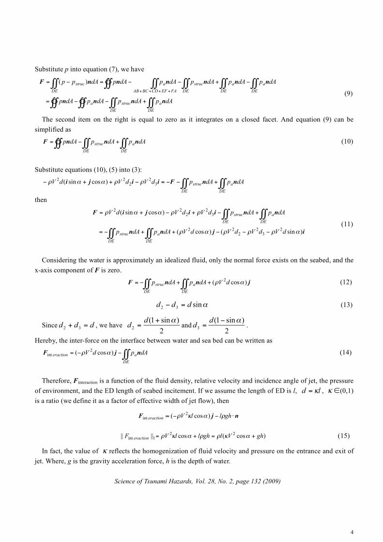
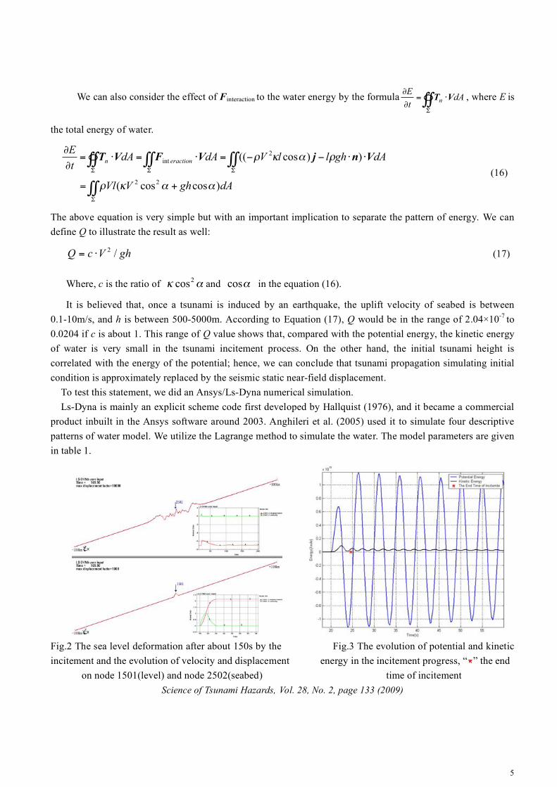
Fig.2 The sea level deformation after about 150s by the Fig.3 The evolution of potential and kinetic

incitement and the evolution of velocity and displacement energy in the incitement progress, “ ” the end

on node 1501(level) and node 2502(seabed) time of incitement


6

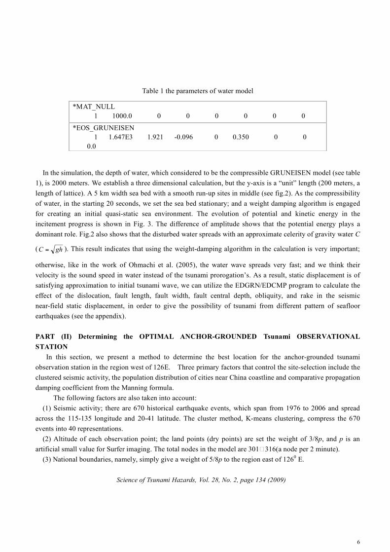
Table 1 the parameters of water model

In the simulation, the depth of water, which considered to be the compressible GRUNEISEN model (see table

1), is 2000 meters. We establish a three dimensional calculation, but the y-axis is a “unit” length (200 meters, a

length of lattice). A 5 km width sea bed with a smooth run-up sites in middle (see fig.2). As the compressibility

of water, in the starting 20 seconds, we set the sea bed stationary; and a weight damping algorithm is engaged

for creating an initial quasi-static sea environment. The evolution of potential and kinetic energy in the

incitement progress is shown in Fig. 3. The difference of amplitude shows that the potential energy plays a

dominant role. Fig.2 also shows that the disturbed water spreads with an approximate celerity of gravity water C

( ghC = ). This result indicates that using the weight-damping algorithm in the calculation is very important;

otherwise, like in the work of Ohmachi et al. (2005), the water wave spreads very fast; and we think their

velocity is the sound speed in water instead of the tsunami prorogation’s. As a result, static displacement is of

satisfying approximation to initial tsunami wave, we can utilize the EDGRN/EDCMP program to calculate the

effect of the dislocation, fault length, fault width, fault central depth, obliquity, and rake in the seismic

near-field static displacement, in order to give the possibility of tsunami from different pattern of seafloor

earthquakes (see the appendix).

PART (II) Determining the OPTIMAL ANCHOR-GROUNDED Tsunami OBSERVATIONAL

STATION

In this section, we present a method to determine the best location for the anchor-grounded tsunami

observation station in the region west of 126E. Three primary factors that control the site-selection include the

clustered seismic activity, the population distribution of cities near China coastline and comparative propagation

damping coefficient from the Manning formula.

The following factors are also taken into account:

(1) Seismic activity; there are 670 historical earthquake events, which span from 1976 to 2006 and spread

across the 115-135 longitude and 20-41 latitude. The cluster method, K-means clustering, compress the 670

events into 40 representations.

(2) Altitude of each observation point; the land points (dry points) are set the weight of 3/8p, and p is an

artificial small value for Surfer imaging. The total nodes in the model are 301� 316(a node per 2 minute).

(3) National boundaries, namely, simply give a weight of 5/8p to the region east of 1260 E.


*MAT_NULL

1 1000.0 0 0 0 0 0 0

*EOS_GRUNEISEN

1 1.647E3 1.921 -0.096 0 0.350 0 0

0.0

7

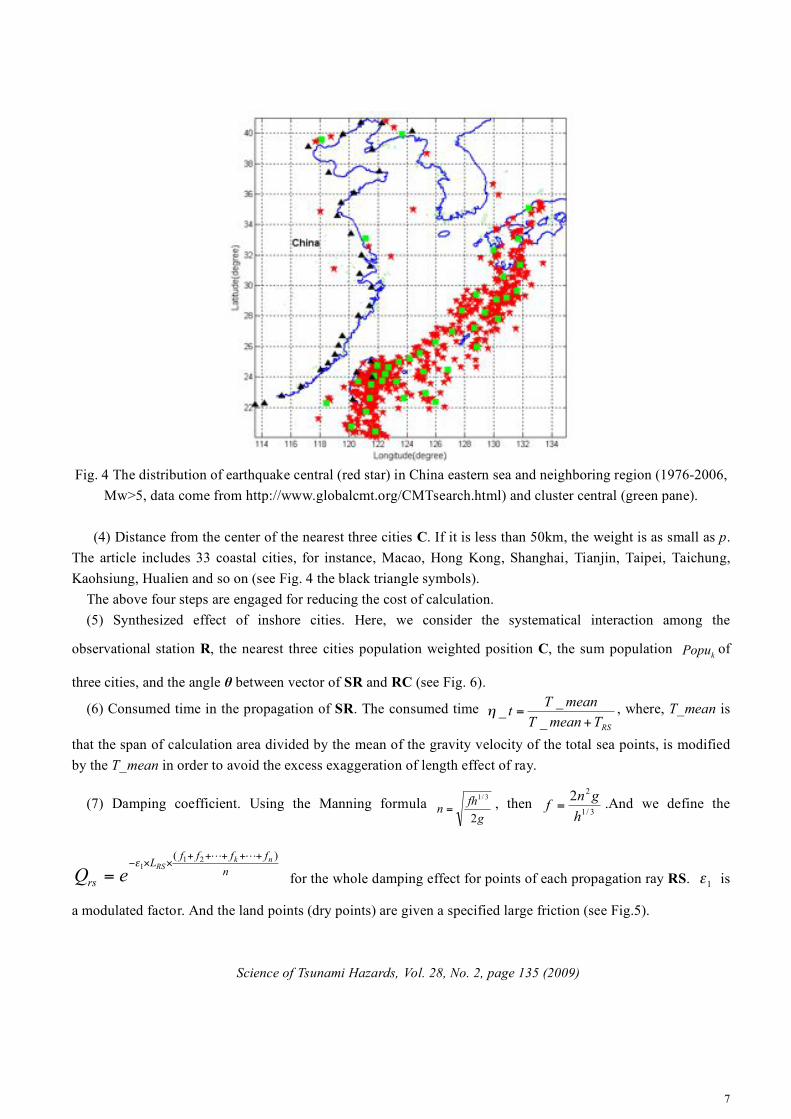
Fig. 4 The distribution of earthquake central (red star) in China eastern sea and neighboring region (1976-2006,

Mw>5, data come from http://www.globalcmt.org/CMTsearch.html) and cluster central (green pane).

(4) Distance from the center of the nearest three cities C. If it is less than 50km, the weight is as small as p.

The article includes 33 coastal cities, for instance, Macao, Hong Kong, Shanghai, Tianjin, Taipei, Taichung,

Kaohsiung, Hualien and so on (see Fig. 4 the black triangle symbols).

The above four steps are engaged for reducing the cost of calculation.

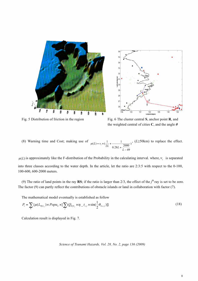
(5) Synthesized effect of inshore cities. Here, we consider the systematical interaction among the

observational station R, the nearest three cities population weighted position C, the sum population kPopu of

three cities, and the angle " between vector of SR and RC (see Fig. 6).

(6) Consumed time in the propagation of SR. The consumed time

RSTmeanT

meanTt

+=

_

__! , where, T_mean is

that the span of calculation area divided by the mean of the gravity velocity of the total sea points, is modified

by the T_mean in order to avoid the excess exaggeration of length effect of ray.

(7) Damping coefficient. Using the Manning formula g

fhn

2

3/1

= , then 3/1

22

h

gnf = .And we define the

n

ffffL

rs

nkRS

eQ

)( 211

+++++!!"

=

LL#

for the whole damping effect for points of each propagation ray RS. 1! is

a modulated factor. And the land points (dry points) are given a specified large friction (see Fig.5).


8

Fig. 5 Distribution of friction in the region Fig. 6 The cluster central S, anchor point R, and

the weighted central of cities C, and the angle "

(8) Warning time and Cost; making use of )

49

200028.0

1

2

1()(

!+

+"=

LL

LvLi

µ, (L"50km) to replace the effect.

)(Lµ is approximately like the F-distribution of the Probability in the calculating interval. where,iv is separated

into three classes according to the water depth. In the article, let the ratio are 2:3:5 with respect to the 0-100,

100-600, 600-2000 meters.

(9) The ratio of land points in the ray RS; if the ratio is larger than 2/3, the effect of the jth

ray is set to be zero.

The factor (9) can partly reflect the contributions of obstacle islands or land in collaboration with factor (7).

The mathematical model eventually is established as follow

})]2

1sin(_([)({ ,,,! ! """"=

k

jik

j

jiSRkCRi tQPopuLPjiki

#$µ (18)

Calculation result is displayed in Fig. 7.


9

0

0.05

0.1

0.15

0.2

0.25

0.3

0.35

0.4

0.45

0.5

0.55

0.6

0.65

0.7

0.75

0.8

1

2

3

4

5

6

7

8

9

10

11

12

13

14

15

16

17

18

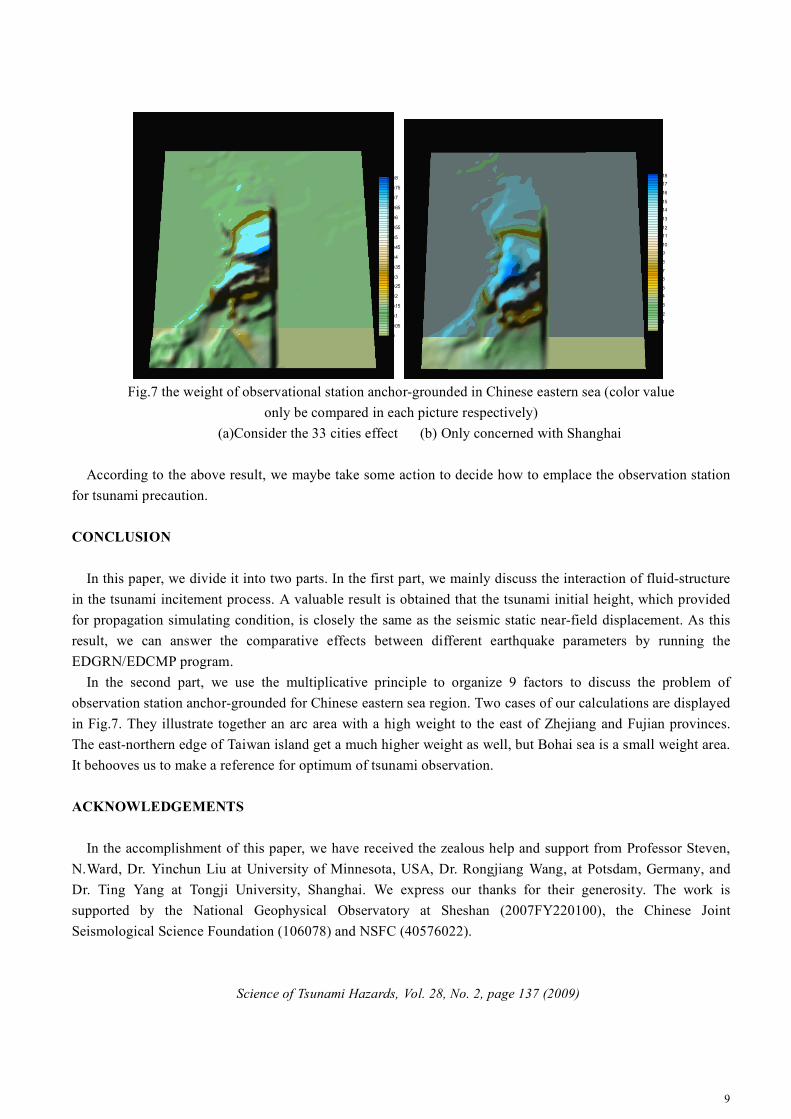
Fig.7 the weight of observational station anchor-grounded in Chinese eastern sea (color value

only be compared in each picture respectively)

(a)Consider the 33 cities effect (b) Only concerned with Shanghai

According to the above result, we maybe take some action to decide how to emplace the observation station

for tsunami precaution.

CONCLUSION

In this paper, we divide it into two parts. In the first part, we mainly discuss the interaction of fluid-structure

in the tsunami incitement process. A valuable result is obtained that the tsunami initial height, which provided

for propagation simulating condition, is closely the same as the seismic static near-field displacement. As this

result, we can answer the comparative effects between different earthquake parameters by running the

EDGRN/EDCMP program.

In the second part, we use the multiplicative principle to organize 9 factors to discuss the problem of

observation station anchor-grounded for Chinese eastern sea region. Two cases of our calculations are displayed

in Fig.7. They illustrate together an arc area with a high weight to the east of Zhejiang and Fujian provinces.

The east-northern edge of Taiwan island get a much higher weight as well, but Bohai sea is a small weight area.

It behooves us to make a reference for optimum of tsunami observation.

ACKNOWLEDGEMENTS

In the accomplishment of this paper, we have received the zealous help and support from Professor Steven,

N.Ward, Dr. Yinchun Liu at University of Minnesota, USA, Dr. Rongjiang Wang, at Potsdam, Germany, and

Dr. Ting Yang at Tongji University, Shanghai. We express our thanks for their generosity. The work is

supported by the National Geophysical Observatory at Sheshan (2007FY220100), the Chinese Joint

Seismological Science Foundation (106078) and NSFC (40576022).


10

APPENDIX

(I) The Effect of Earthquake Parameters

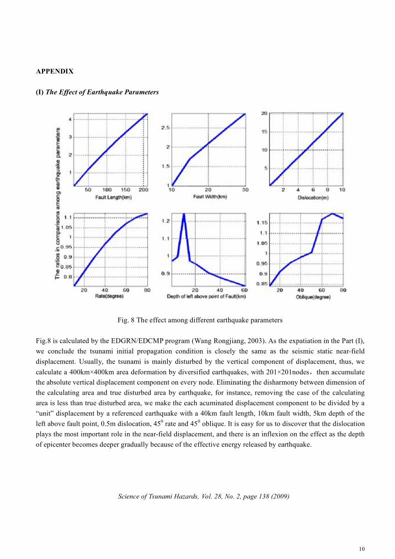
Fig. 8 The effect among different earthquake parameters

Fig.8 is calculated by the EDGRN/EDCMP program (Wang Rongjiang, 2003). As the expatiation in the Part (I),

we conclude the tsunami initial propagation condition is closely the same as the seismic static near-field

displacement. Usually, the tsunami is mainly disturbed by the vertical component of displacement, thus, we

calculate a 400km!400km area deformation by diversified earthquakes, with 201!201nodes!then accumulate

the absolute vertical displacement component on every node. Eliminating the disharmony between dimension of

the calculating area and true disturbed area by earthquake, for instance, removing the case of the calculating

area is less than true disturbed area, we make the each acuminated displacement component to be divided by a

“unit” displacement by a referenced earthquake with a 40km fault length, 10km fault width, 5km depth of the

left above fault point, 0.5m dislocation, 450 rate and 45

0 oblique. It is easy for us to discover that the dislocation

plays the most important role in the near-field displacement, and there is an inflexion on the effect as the depth

of epicenter becomes deeper gradually because of the effective energy released by earthquake.


11

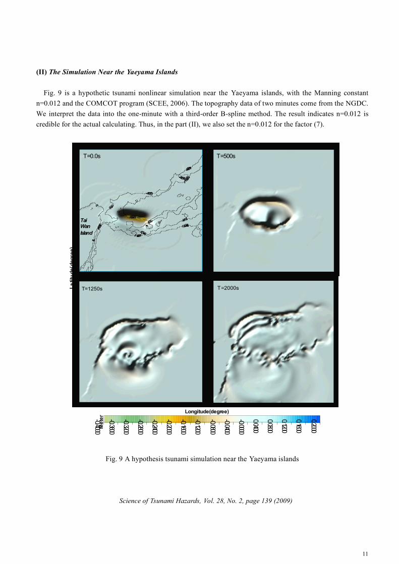
(II) The Simulation Near the Yaeyama Islands

Fig. 9 is a hypothetic tsunami nonlinear simulation near the Yaeyama islands, with the Manning constant

n=0.012 and the COMCOT program (SCEE, 2006). The topography data of two minutes come from the NGDC.

We interpret the data into the one-minute with a third-order B-spline method. The result indicates n=0.012 is

credible for the actual calculating. Thus, in the part (II), we also set the n=0.012 for the factor (7).

-0 .4 000

- 0. 36 00

- 0. 32 00

-0 .28 00

-0 .2 400

- 0. 200 0

- 0. 160 0

- 0. 120 0

- 0. 080 0

- 0. 040 0

-0 .0 000

0. 040 0

0. 080 0

0 .120 0

0. 160 0

0 .20 00

T=0.0s T=500s

T=1250s T=2000s

Tai

Wan

Island

Longitude(degree)

Latitude(degree)

Met er

Fig. 9 A hypothesis tsunami simulation near the Yaeyama islands


12

REFERENCES

[1] Carlo Brandini, Stéphan T. Grilli.(2001). Modeling of freak wave generation in a 3D-NWT, To appear in

Proc.ISOPE 2001 Conf. Stavanger, Norway (http://www.oce.uri.edu/~grilli/isope13.pdf)

[2] Gutenberg, B. (1939). Tsunamis and earthquakes, Bull, seism, Soc.America. 29:4, 517-526

[3] John O.Hallquist (2006). LS-DYN A theory manual

[4] Kajiura, K (1970). Tsunami Source, Energy and the Directivity of Wave Radiation, Bulletin of the

Earthquake Research Institute, Vol.48, 835-869

[5] M.D. Trifunac, A. Hayir, M.I. Todorovska. (2003). A note on tsunami caused by submarine slides and

slumps spreading in one dimension with non-uniform displacement amplitudes, Soil Dynamics and Earthquake

Engineering Vol.23, 223-234

[6] Maria I. Todorovska, Mihailo D. Trifunac (2001). Generation of tsunamis by a slowly spreading uplift of the

sea floor, Soil Dynamics and Earthquake Engineering Vol.21, 151-167

[7] M.I.Todorovska, A.Hayir, M.D.Trifunac (2002). A note on tsunami amplitudes above submarine slides and

slumps, Soil Dynamics and Earthquake Engineering Vol.22, 129-141

[8] Philip Watts, Stephan T. Grilli, M. Asce (2005). David R. Tappin and Gerard J.Fryer, Tsunami Generation

by Submarine Mass Failure II: Predictive Equations and Case Studies, Journal of Waterway, Port, Coastal, and

Ocean Engineering, Vol.131, No.6, November 1

[9] P.L.-F Liu, T. -R. Wu, F. Raichlen et al. (2005). Run-up and rundown generated by three-dimensional

sliding masses, J. Fluid. Mech, 107-144

[10] Rongjiang Wang et al. (2003). Computation of deformation induced by earthquakes in a multi-layered

elastic crust—FORTRAN programs EDGRN/EDCMP, Computers & Geosciences Vol.29 (2003), 195-207

[11] SCEE (School of Civil and Environmental Engineering, Cornell University)(2006). COMCOT User

Manual, Version 1.6

[12] Stéphan T. Grilli, Richard W. Gilbert (2004). Pierre Lubin et al., Numerical Modeling and Experiments for

Solitary Wave Shoaling and Breaking over a Sloping Beach, Proceedings of The Thirteenth (2004) International

Offshore and Polar Engineering Conference Toulon, France, May23-28, 2004, 306-312

[13] Steven N. Ward (2003). Classical Tsunami Theory-a la Ward


13

[14] Steven N.Ward. Tsunamis in The Encyclopedia of Physical Science and Technology, ed. R. A. Meyers,

Academic Press, Vol. 17, 175-191

[15] Tatsuo Ohmachi et al. (2001). Simulation of Tsunami Induced by Dynamic displacement of Seabed due to

Seismic Faulting, Bulletin of Seismological Society of America, 91:6, 1898-1909


Documents

A New Method to Analyze the Tsunami Incitement Process …tsunamisociety.org/282Zhub.pdf · 1 A New Method to Analyze the Tsunami Incitement Process and Site-selection for Tsunami