A New MIP Model for Parallel-BatchScheduling with Non-Identical Job Sizes

Sebastian Kosch and J. Christopher Beck

Department of Mechanical & Industrial EngineeringUniversity of Toronto, Toronto, Ontario M5S 3G8, Canada

{skosch,jcb}@mie.utoronto.ca

Abstract. Parallel-batch machine problems arise in numerous manu-facturing settings from semiconductor manufacturing to printing. Theyhave recently been addressed in constraint programming (CP) via thecombination of the novel sequenceEDD global constraint with the exist-ing pack constraint to form the current state-of-the-art approach. In thispaper, we present a detailed analysis of the problem and derivation of anumber of properties that are exploited in a novel mixed integer program-ming (MIP) model for the problem. Our empirical results demonstratethat the new model is able to outperform the CP model across a range ofstandard benchmark problems. Further investigation shows that the newMIP formulation improves on the existing formulation primarily by pro-ducing a much smaller model and enabling high quality primal solutionsto be found very quickly.

1 Introduction

Despite the widespread application of mixed integer programming (MIP) tech-nology to optimization problems in general and scheduling problems specifi-cally,1 there is a significant body of work that demonstrates the superiority ofconstraint programming (CP) and hybrid approaches for a number of classesof scheduling problems [1–5]. While the superiority is often a result of stronginference techniques embedded in global constraints [6–8], it is sometimes due toproblem-specific implementation in the form of specialized global constraints [4]or instantiations of decomposition techniques [1–3]. The flexibility of CP and de-composition approaches which facilitates such implementations is undoubtedlypositive from the perspective of solving specific problems better. However, theability to create problem-specific approaches is in some ways in opposition tothe compositionality and model-and-solve “holy grail” of CP [9]: to enable usersto model and solve problems without implementing anything new at all.

Our overarching thesis is that, in fact, MIP technology is closer to this goalthan CP, at least in the context of combinatorial optimization problems. Inour investigation of this thesis, we are developing MIP models for scheduling

1 For example, of the 58 papers published in the Journal of Scheduling in 2012, 19 useMIP, more than any other single approach.

problems where the current state of the art is customized CP or hybrid ap-proaches. Heinz et al. [10] showed that on a class of resource allocation andscheduling problems, a MIP model could be designed that was competitive withthe state-of-the-art logic-based Benders decomposition. This paper represents asimilar contribution in different scheduling problem: a parallel-batch processingproblem which has previously been attacked by MIP, branch-and-price [11], andCP [4] with the latter representing the state of the art.

We propose a MIP model inspired by the idea of modifying a canonical fea-sible solution. The definition of our objective function in this novel context isnot intuitive until we reason algorithmically about how constraints and assign-ments interact – a strategy often used in designing metaheuristics. Indeed, wesuggest that the analogy between branching on independent decision variablesand making moves between neighbouring schedules should be explored in moredetail for a range of combinatorial problems.

In the next section we present the formal problem definition and discussexisting approaches. In Section 3 we prove a number of propositions that allowus to formally propose a novel MIP model for the problem in Section 4. Section5 presents our empirical results, demonstrating that the performance of the newmodel is superior to the existing CP model, both in terms of mean time to findoptimal solutions and in terms of solution quality when optimal solutions couldnot be found within the time limit.

2 Background

Batch machines with limited capacity exist in many manufacturing settings informs such as ovens [12], autoclaves [4], and tanks [13]. In this paper, we tacklethe problem of minimizing the maximum lateness, Lmax, in a single machineparallel batching problem where each job has an individual due date and size.

We use the following notation: a set J of n jobs is to be assigned to a set ofn batches B = {B1, . . . , Bn}. Batches can hold multiple jobs or remain empty.Each job j has a processing time, pj , a size, sj , and a due date, dj . Jobs canbe assigned to arbitrary batches, as long as the sum of the sizes of the jobs in abatch does not exceed the machine capacity, b.

The single machine processes one batch at a time. Each batch Bk has a batchstart date Sk, a batch processing time, defined as the longest processing time ofall jobs assigned to the batch, Pk = maxj∈Bk

(pj), and a batch completion date,which must fall before the start time of the next batch, Ck = Sk + Pk ≤ Sk+1.

The lateness of a job j, Lj , is the completion time of its batch Ck less itsdue date dj . The objective function is to minimize the maximum lateness overall jobs, Lmax = maxj∈J (Lj). Since we are interested in the maximum lateness,only the earliest-due job in each batch matters and we define it as the batch duedate Dk = minj∈Bk

(dj).

The problem can be summarized as 1|p-batch; b < n; non-identical|Lmax [4,11], where p-batch; b < n represents the resource’s parallel-batch nature and

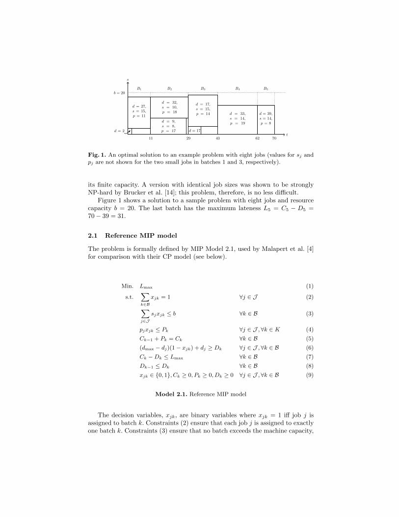
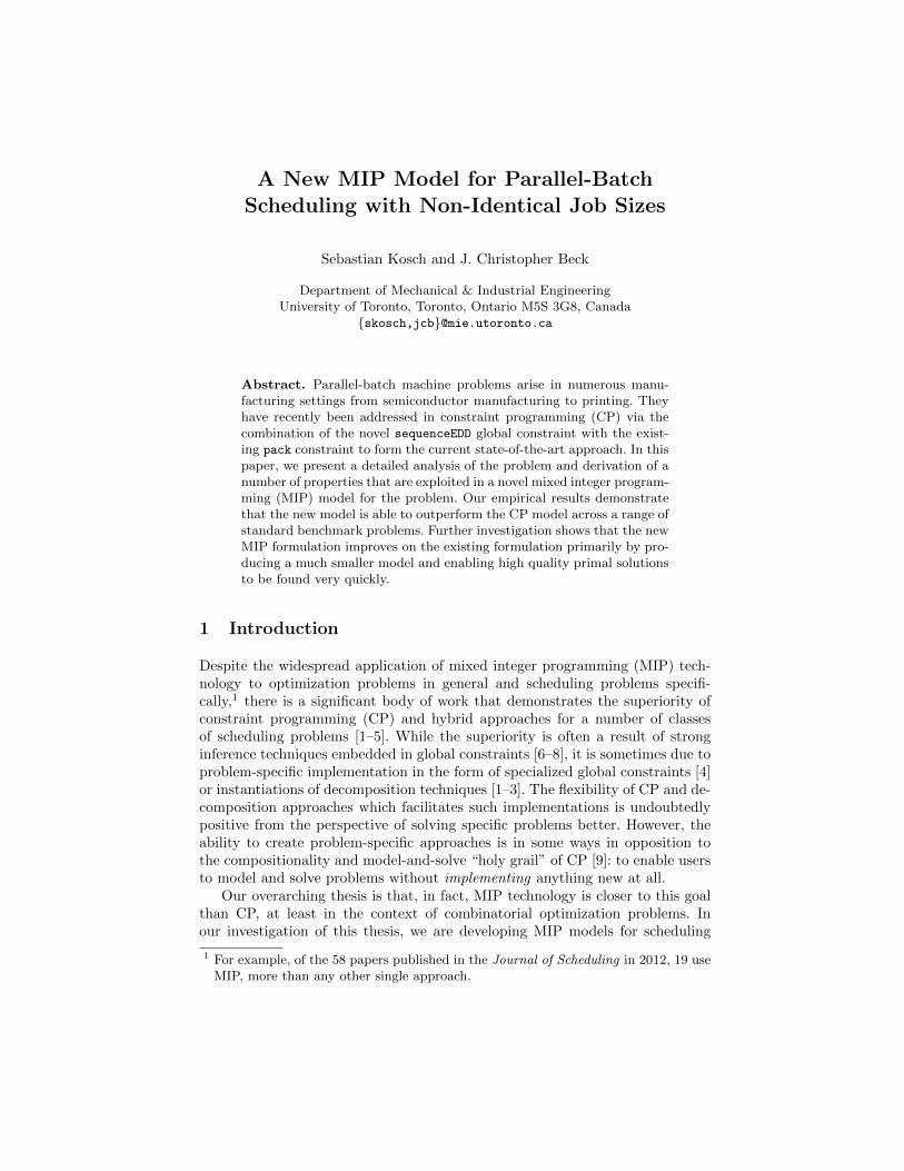
Fig. 1. An optimal solution to an example problem with eight jobs (values for sj andpj are not shown for the two small jobs in batches 1 and 3, respectively).

its finite capacity. A version with identical job sizes was shown to be stronglyNP-hard by Brucker et al. [14]; this problem, therefore, is no less difficult.

Figure 1 shows a solution to a sample problem with eight jobs and resourcecapacity b = 20. The last batch has the maximum lateness L5 = C5 − D5 =70− 39 = 31.

2.1 Reference MIP model

The problem is formally defined by MIP Model 2.1, used by Malapert et al. [4]for comparison with their CP model (see below).

Min. Lmax (1)

s.t.∑k∈B

xjk = 1 ∀j ∈ J (2)

∑j∈J

sjxjk ≤ b ∀k ∈ B (3)

pjxjk ≤ Pk ∀j ∈ J ,∀k ∈ K (4)

Ck−1 + Pk = Ck ∀k ∈ B (5)

(dmax − dj)(1− xjk) + dj ≥ Dk ∀j ∈ J ,∀k ∈ B (6)

Ck −Dk ≤ Lmax ∀k ∈ B (7)

Dk−1 ≤ Dk ∀k ∈ B (8)

xjk ∈ {0, 1}, Ck ≥ 0, Pk ≥ 0, Dk ≥ 0 ∀j ∈ J ,∀k ∈ B (9)

Model 2.1. Reference MIP model

The decision variables, xjk, are binary variables where xjk = 1 iff job j isassigned to batch k. Constraints (2) ensure that each job j is assigned to exactlyone batch k. Constraints (3) ensure that no batch exceeds the machine capacity,

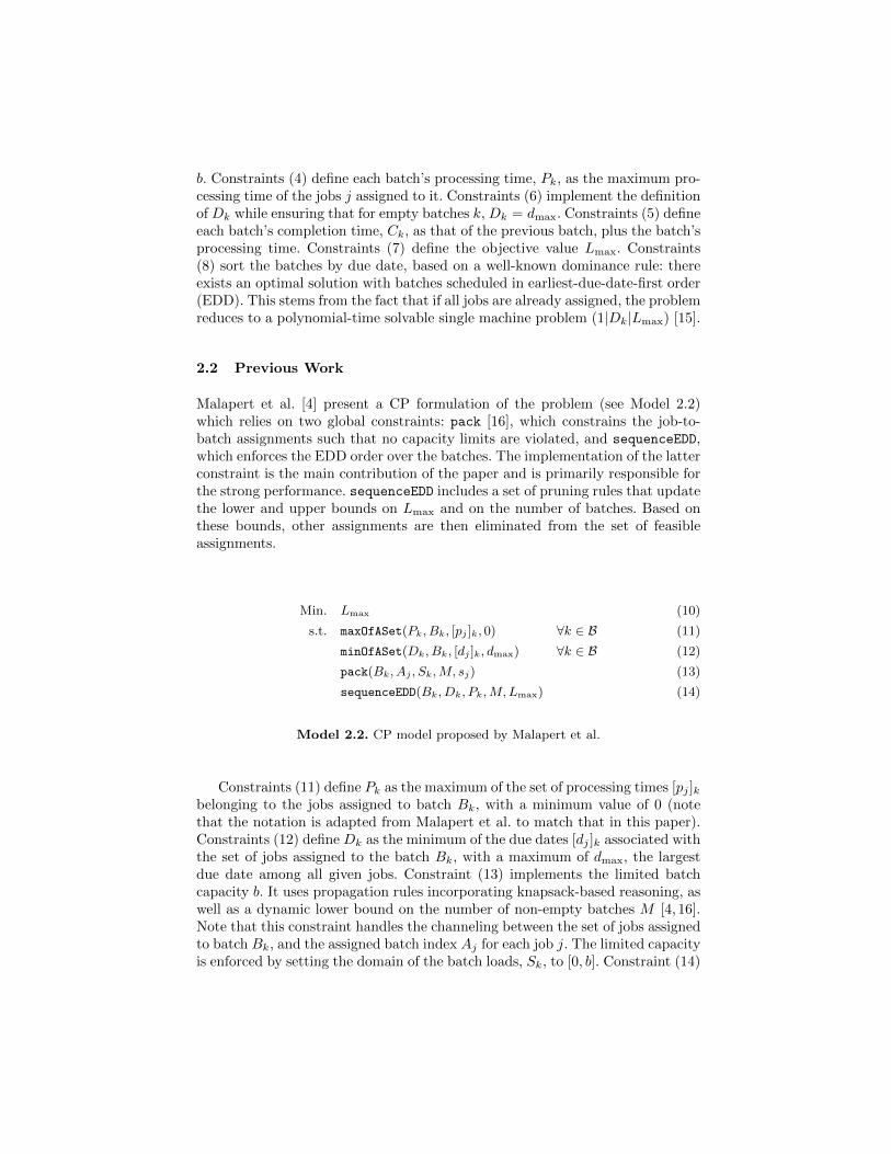
b. Constraints (4) define each batch’s processing time, Pk, as the maximum pro-cessing time of the jobs j assigned to it. Constraints (6) implement the definitionof Dk while ensuring that for empty batches k, Dk = dmax. Constraints (5) defineeach batch’s completion time, Ck, as that of the previous batch, plus the batch’sprocessing time. Constraints (7) define the objective value Lmax. Constraints(8) sort the batches by due date, based on a well-known dominance rule: thereexists an optimal solution with batches scheduled in earliest-due-date-first order(EDD). This stems from the fact that if all jobs are already assigned, the problemreduces to a polynomial-time solvable single machine problem (1|Dk|Lmax) [15].

2.2 Previous Work

Malapert et al. [4] present a CP formulation of the problem (see Model 2.2)which relies on two global constraints: pack [16], which constrains the job-to-batch assignments such that no capacity limits are violated, and sequenceEDD,which enforces the EDD order over the batches. The implementation of the latterconstraint is the main contribution of the paper and is primarily responsible forthe strong performance. sequenceEDD includes a set of pruning rules that updatethe lower and upper bounds on Lmax and on the number of batches. Based onthese bounds, other assignments are then eliminated from the set of feasibleassignments.

Min. Lmax (10)

s.t. maxOfASet(Pk, Bk, [pj ]k, 0) ∀k ∈ B (11)

minOfASet(Dk, Bk, [dj ]k, dmax) ∀k ∈ B (12)

pack(Bk, Aj , Sk,M, sj) (13)

sequenceEDD(Bk, Dk, Pk,M,Lmax) (14)

Model 2.2. CP model proposed by Malapert et al.

Constraints (11) define Pk as the maximum of the set of processing times [pj ]kbelonging to the jobs assigned to batch Bk, with a minimum value of 0 (notethat the notation is adapted from Malapert et al. to match that in this paper).Constraints (12) define Dk as the minimum of the due dates [dj ]k associated withthe set of jobs assigned to the batch Bk, with a maximum of dmax, the largestdue date among all given jobs. Constraint (13) implements the limited batchcapacity b. It uses propagation rules incorporating knapsack-based reasoning, aswell as a dynamic lower bound on the number of non-empty batches M [4, 16].Note that this constraint handles the channeling between the set of jobs assignedto batch Bk, and the assigned batch index Aj for each job j. The limited capacityis enforced by setting the domain of the batch loads, Sk, to [0, b]. Constraint (14)

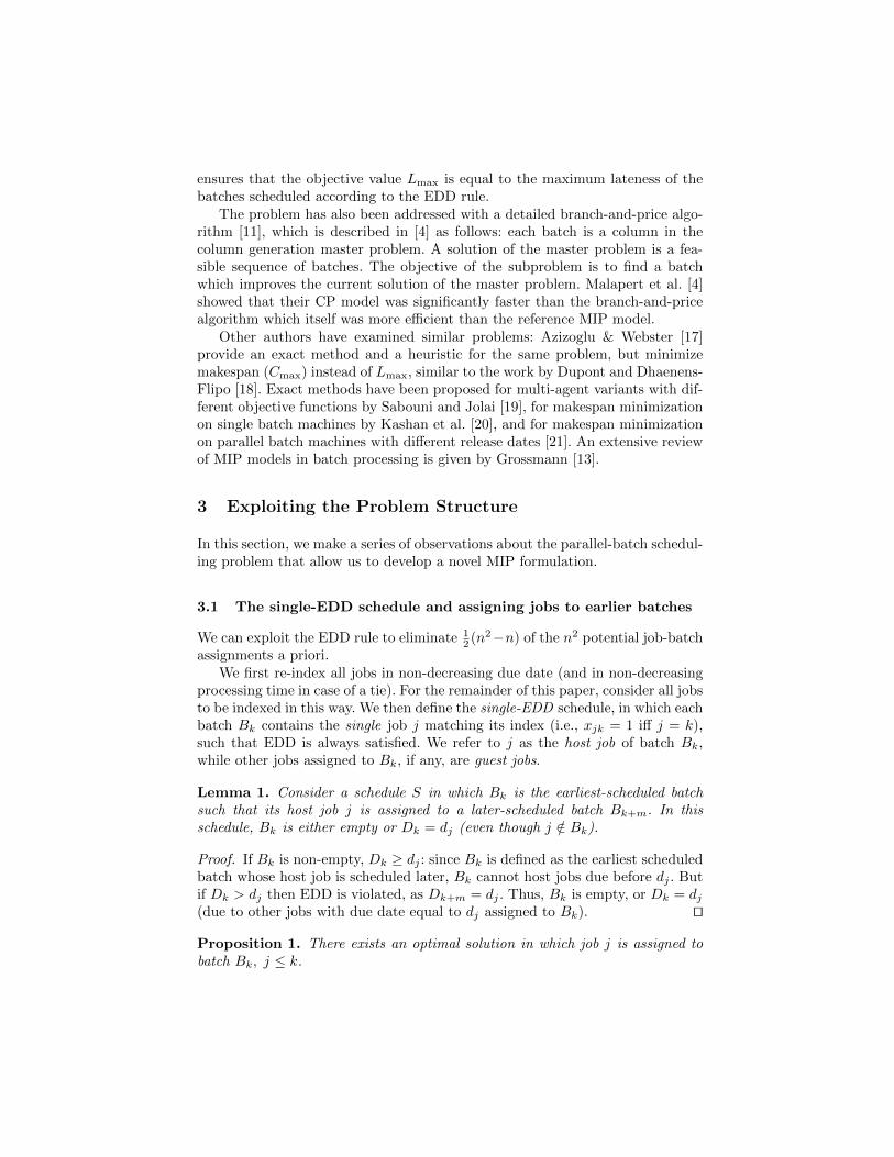
ensures that the objective value Lmax is equal to the maximum lateness of thebatches scheduled according to the EDD rule.

The problem has also been addressed with a detailed branch-and-price algo-rithm [11], which is described in [4] as follows: each batch is a column in thecolumn generation master problem. A solution of the master problem is a fea-sible sequence of batches. The objective of the subproblem is to find a batchwhich improves the current solution of the master problem. Malapert et al. [4]showed that their CP model was significantly faster than the branch-and-pricealgorithm which itself was more efficient than the reference MIP model.

Other authors have examined similar problems: Azizoglu & Webster [17]provide an exact method and a heuristic for the same problem, but minimizemakespan (Cmax) instead of Lmax, similar to the work by Dupont and Dhaenens-Flipo [18]. Exact methods have been proposed for multi-agent variants with dif-ferent objective functions by Sabouni and Jolai [19], for makespan minimizationon single batch machines by Kashan et al. [20], and for makespan minimizationon parallel batch machines with different release dates [21]. An extensive reviewof MIP models in batch processing is given by Grossmann [13].

3 Exploiting the Problem Structure

In this section, we make a series of observations about the parallel-batch schedul-ing problem that allow us to develop a novel MIP formulation.

3.1 The single-EDD schedule and assigning jobs to earlier batches

We can exploit the EDD rule to eliminate 12 (n2−n) of the n2 potential job-batch

assignments a priori.We first re-index all jobs in non-decreasing due date (and in non-decreasing

processing time in case of a tie). For the remainder of this paper, consider all jobsto be indexed in this way. We then define the single-EDD schedule, in which eachbatch Bk contains the single job j matching its index (i.e., xjk = 1 iff j = k),such that EDD is always satisfied. We refer to j as the host job of batch Bk,while other jobs assigned to Bk, if any, are guest jobs.

Lemma 1. Consider a schedule S in which Bk is the earliest-scheduled batchsuch that its host job j is assigned to a later-scheduled batch Bk+m. In thisschedule, Bk is either empty or Dk = dj (even though j /∈ Bk).

Proof. If Bk is non-empty, Dk ≥ dj : since Bk is defined as the earliest scheduledbatch whose host job is scheduled later, Bk cannot host jobs due before dj . Butif Dk > dj then EDD is violated, as Dk+m = dj . Thus, Bk is empty, or Dk = dj(due to other jobs with due date equal to dj assigned to Bk). ut

Proposition 1. There exists an optimal solution in which job j is assigned tobatch Bk, j ≤ k.

Proof. Consider again schedule S. Since Dk+m = dj , EDD requires that no batchBq, k ≤ q < k + m, is due after dj . By Lemma 1, we only need to consider thefollowing two cases:

1. Bk is empty, so Pk = 0. Since EDD is not violated, we know that Dq =dj ∀ Bq, k ≤ q ≤ k + m. We can assign all jobs from Bk+m to Bk, suchthat Pk+m = 0. Lmax will stay constant, as the completion time of the last-scheduled of all batches due at dj does not change.

2. Bk is non-empty and due at Dk = dj (although j /∈ Bk), due to at leastone job g from a later-scheduled batch for which dg = dj , which is assignedto Bk. In this case, since Dk = dj = Dk+m and since EDD is not violated,all batches Bq where k ≤ q ≤ k + m must be due at dj . But then we canre-order these batches such that their respective earliest-due jobs are onceagain assigned to their single-EDD indices. The jobs in Bk+m (including j)will be assigned to Bk as a result. Lmax is not affected by this re-assignment,as the completion time of the last-scheduled batch due at dj does not change.

ut

We thus introduce the following constraint to exclude solutions in which jobsare assigned to later batches than their single-EDD batches.

xjk = 0 ∀{j ∈ J , k ∈ B|j < k} (15)

We can also show that in every non-empty batch Bk, the earliest-due job jmust be the host job. This means that when batch Bk’s host job is assigned toan earlier batch, no other jobs can be assigned to Bk; a batch that is hostlessmust be empty. This requirement rests on the following proposition.

Proposition 2. There exists an optimal solution that has no hostless, non-empty batches.

Proof. Consider an EDD-ordered schedule in which batch Bj is the last-scheduledbatch which is hostless but non-empty: instead of its host job, only a set G oflater-due guest jobs is assigned to Bj (j /∈ G).

The earliest-due job g ∈ G must have the same due date as batch Bj+1: if itis due later, EDD is violated; if it is due earlier, G is not a set of later-due guestjobs. Job g’s own host batch Bg (which is hostless) cannot itself be due laterthan dg = Dj+1 – this would require Bg to have guest jobs from later batches,but we defined Bk as the last batch with this property – therefore, Dq = Dj+1

for all batches Bq, j ≤ q ≤ g.Then we can re-assign the guest jobs G from Bj into Bg, such that g is again

host job in its own single-EDD batch. This re-assignment has no impact on Lmax

since it makes Pj = 0, resulting in the same completion time of the set of allbatches with batch due date D = Dj+1. ut

The above proposition translates to the following constraint:

xkk ≥ xjk ∀{j ∈ J , k ∈ B|j > k} (16)

This observation allows us to define the due date of all batches to be the duedate of their respective host jobs: Dk = dj , ∀{j ∈ J , k ∈ B|j = k}. This ruleholds even for empty batches Bk: Pk = 0, so Ck = Ck−1; but Dk−1 ≤ Dk due tothis rule, so Lk−1 ≥ Lk and thus Lk has no impact on Lmax.

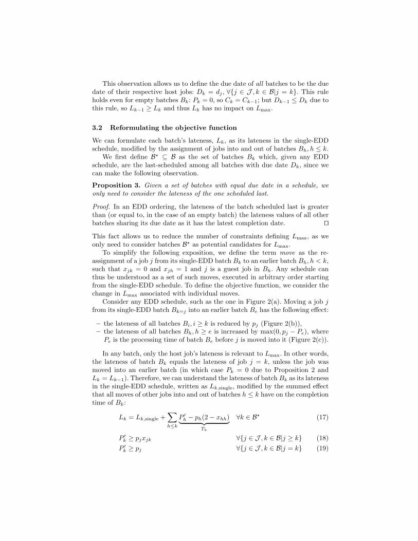
3.2 Reformulating the objective function

We can formulate each batch’s lateness, Lk, as its lateness in the single-EDDschedule, modified by the assignment of jobs into and out of batches Bh, h ≤ k.

We first define B? ⊆ B as the set of batches Bk which, given any EDDschedule, are the last-scheduled among all batches with due date Dk, since wecan make the following observation.

Proposition 3. Given a set of batches with equal due date in a schedule, weonly need to consider the lateness of the one scheduled last.

Proof. In an EDD ordering, the lateness of the batch scheduled last is greaterthan (or equal to, in the case of an empty batch) the lateness values of all otherbatches sharing its due date as it has the latest completion date. ut

This fact allows us to reduce the number of constraints defining Lmax, as weonly need to consider batches B? as potential candidates for Lmax.

To simplify the following exposition, we define the term move as the re-assignment of a job j from its single-EDD batch Bk to an earlier batch Bh, h < k,such that xjk = 0 and xjh = 1 and j is a guest job in Bh. Any schedule canthus be understood as a set of such moves, executed in arbitrary order startingfrom the single-EDD schedule. To define the objective function, we consider thechange in Lmax associated with individual moves.

Consider any EDD schedule, such as the one in Figure 2(a). Moving a job jfrom its single-EDD batch Bk=j into an earlier batch Be has the following effect:

– the lateness of all batches Bi, i ≥ k is reduced by pj (Figure 2(b)),– the lateness of all batches Bh, h ≥ e is increased by max(0, pj − Pe), where

Pe is the processing time of batch Be before j is moved into it (Figure 2(c)).

In any batch, only the host job’s lateness is relevant to Lmax. In other words,the lateness of batch Bk equals the lateness of job j = k, unless the job wasmoved into an earlier batch (in which case Pk = 0 due to Proposition 2 andLk = Lk−1). Therefore, we can understand the lateness of batch Bk as its latenessin the single-EDD schedule, written as Lk,single, modified by the summed effectthat all moves of other jobs into and out of batches h ≤ k have on the completiontime of Bk:

Lk = Lk,single +∑h≤k

P ′h − ph(2− xhh)︸ ︷︷ ︸Th

∀k ∈ B? (17)

P ′k ≥ pjxjk ∀{j ∈ J , k ∈ B|j ≥ k} (18)

P ′k ≥ pj ∀{j ∈ J , k ∈ B|j = k} (19)

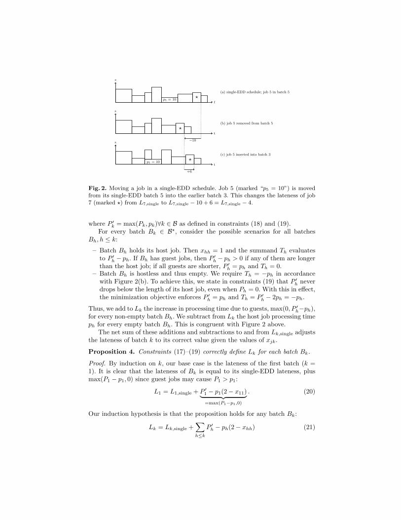
Fig. 2. Moving a job in a single-EDD schedule. Job 5 (marked “p5 = 10”) is movedfrom its single-EDD batch 5 into the earlier batch 3. This changes the lateness of job7 (marked ?) from L7,single to L7,single − 10 + 6 = L7,single − 4.

where P ′k = max(Pk, pk)∀k ∈ B as defined in constraints (18) and (19).For every batch Bk ∈ B?, consider the possible scenarios for all batches

Bh, h ≤ k:

– Batch Bh holds its host job. Then xhh = 1 and the summand Th evaluatesto P ′h − ph. If Bh has guest jobs, then P ′h − ph > 0 if any of them are longerthan the host job; if all guests are shorter, P ′h = ph and Th = 0.

– Batch Bh is hostless and thus empty. We require Th = −ph in accordancewith Figure 2(b). To achieve this, we state in constraints (19) that P ′h neverdrops below the length of its host job, even when Ph = 0. With this in effect,the minimization objective enforces P ′h = ph and Th = P ′h − 2ph = −ph.

Thus, we add to Lk the increase in processing time due to guests, max(0, P ′h−ph),for every non-empty batch Bh. We subtract from Lk the host job processing timeph for every empty batch Bh. This is congruent with Figure 2 above.

The net sum of these additions and subtractions to and from Lk,single adjuststhe lateness of batch k to its correct value given the values of xjk.

Proposition 4. Constraints (17)–(19) correctly define Lk for each batch Bk.

Proof. By induction on k, our base case is the lateness of the first batch (k =1). It is clear that the lateness of Bk is equal to its single-EDD lateness, plusmax(P1 − p1, 0) since guest jobs may cause P1 > p1:

L1 = L1,single + P ′1 − p1(2− x11)︸ ︷︷ ︸=max(P1−p1,0)

. (20)

Our induction hypothesis is that the proposition holds for any batch Bk:

Lk = Lk,single +∑h≤k

P ′h − ph(2− xhh) (21)

To show how an expression for Lk+1 then follows, we relate Lk+1 to Lk:

Lk+1 = Lk + Pk+1︸ ︷︷ ︸Ck+1−Ck

− (dk+1 − dk)︸ ︷︷ ︸Dk+1−Dk

(22)

The difference Lk+1 − Lk can also be written in terms of single-EDD latenessvalues and processing time adjustments due to guests or hostlessness, all of whichare expressed in known terms:

Pk+1−(dk+1−dk) = Lk+1,single−Lk,single+

{max(Pk+1 − pk+1, 0) xk+1,k+1 = 1

−pk+1 xk+1,k+1 = 0.

(23)The conditional expression is equivalent to P ′k+1 − pk+1(2 − xk+1,k+1). We cannow rewrite (22) for Lk+1 and arrive at

Lk+1 =

Lk,single +∑h≤k

P ′h − ph(2− xhh)

+ Lk+1,single − Lk,single + P ′k+1 − pk+1(2− xk+1,k+1), (24)

which, after cancelling out Lk,single terms, becomes

Lk+1 = Lk+1,single +∑

h≤k+1

P ′h − ph(2− xhh) (25)

and agrees with (21). Since (25) follows from (21), and the latter is true for thebase case of k = 1, (17) is true for all k. ut

Note also that in the case of an empty batch Bk ∈ B?, if Bk−1 /∈ B?, dk =dk−1 and xkk = 0, so Lk = Lk−1 as evident from (24); if Bk−1 ∈ B?, dk > dk−1,and thus Lk < Lk−1. as dk = dk−1 and xkk = 0 if Bk is empty.

3.3 Additional lazy constraints

Lazy constraints [22] are also used in the model. Lazy constraints are constraintsbased on the specific problem instance. Large numbers of them are generatedprior to solving, but they are not immediately used in the model. Instead, theyare checked against whenever an integral solution is found, and only those thatare violated are added to the LP model. In practice, only few of the lazy con-straints are used in the solution process. Nevertheless, they can noticeably im-prove solving time in some cases.

Symmetry-breaking rule This rule creates an explicit, arbitrary preferencefor certain solutions. Consider two schedules S1 and S2. Both schedules containbatches Bh and Bk, both of which are holding their respective host jobs only.

Two jobs j and i are now assigned as the only guests to the two batches; further-more max(pi, pj) ≤ min(ph, pk), max(sh, sk) + max(sj , si) ≤ b and min(dj , di) ≥max(dh, dk). If j ∈ Bh and i ∈ Bk in schedule S1 and vice versa in S2, then theconstraint renders S2 infeasible.

2(4− xhh − xkk − xjh − xjk − xih − xik

+∑g

g 6=jg 6=i

(xgh + xgk)) ≥ xjk + xih

∀{j, i ∈ J ,h, k ∈ B

| h < k < j < i∧[pq ≤ pr ∧ b− sr ≥ sq

∀q ∈ {j, i},∀r ∈ {h, k}]}

(26)

The left-hand side of the equation evaluates to zero exactly when the aboveconditions are met, which in turn disallows the assignment given on the right.For all other job/batch pairings, the left side evaluates to at least two, whichplaces no constraint on the right hand side.

This kind of symmetry-breaking rule can be extended to m > 2 batches,with the number of constraints growing combinatorially with m. Since it takesa constant but appreciable time to generate these constraints prior to solving,we have in our trials kept to the simplest variant shown here, and limited theiruse to problem instances with n ≥ 50 jobs.

Dominance rule on required assignments A schedule is not uniquely opti-mal if a job j is left in its single-EDD batch although there is capacity for it inan earlier batch. This constraint can be expressed logically as: if a job j can besafely assigned to Bk without violating the capacity constraint, then j must beassigned to any earlier batch, or Bk must be empty (or both).

The left side of the above if-then statement is written as (1.0 + b − sj −∑nj

i=ki 6=j

sixik)/b, which evaluates to 1.0 or greater iff sk plus the sizes of guest jobs

in k sum to less than b− sj . The constraint is written as follows:

2− xjj − xkk ≥

1.0 + b− sj −nj∑i=ki 6=j

sixik

/b

∀{j ∈ J , k ∈ B|j > k ∧ pk ≥ pj

∧sk + sj ≤ b}(27)

As with the rule above, we have found that only more difficult problems withn ≥ 50 benefit from these constraints.

4 A New MIP Model

The full novel MIP model we are proposing is defined in Model 4.1.

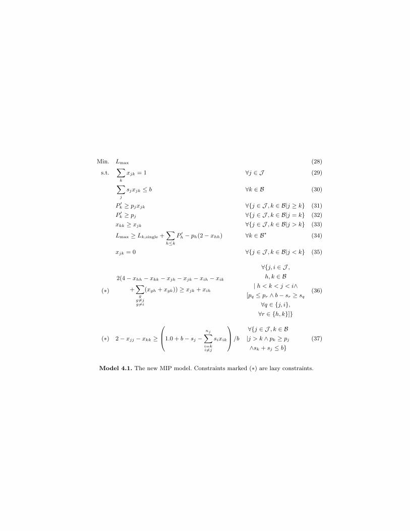
Min. Lmax (28)

s.t.∑k

xjk = 1 ∀j ∈ J (29)∑j

sjxjk ≤ b ∀k ∈ B (30)

P ′k ≥ pjxjk ∀{j ∈ J , k ∈ B|j ≥ k} (31)

P ′k ≥ pj ∀{j ∈ J , k ∈ B|j = k} (32)

xkk ≥ xjk ∀{j ∈ J , k ∈ B|j > k} (33)

Lmax ≥ Lk,single +∑h≤k

P ′h − ph(2− xhh) ∀k ∈ B? (34)

xjk = 0 ∀{j ∈ J , k ∈ B|j < k} (35)

(∗)

2(4− xhh − xkk − xjh − xjk − xih − xik

+∑g

g 6=jg 6=i

(xgh + xgk)) ≥ xjk + xih

∀{j, i ∈ J ,h, k ∈ B

| h < k < j < i∧[pq ≤ pr ∧ b− sr ≥ sq

∀q ∈ {j, i},∀r ∈ {h, k}]}

(36)

(∗) 2− xjj − xkk ≥

1.0 + b− sj −nj∑i=ki 6=j

sixik

/b

∀{j ∈ J , k ∈ B|j > k ∧ pk ≥ pj

∧sk + sj ≤ b}(37)

Model 4.1. The new MIP model. Constraints marked (∗) are lazy constraints.

Constraints (29) and (30) are uniqueness and capacity constraints: batcheshave to remain within capacity b, and every job can only occupy one batch.Constraints (31) and (32) define the value of P ′k for every batch k as the longestp of all jobs in k, but at least pk. This is required in (34), which follows theexplanation above. Constraints (33) ensure that no job is moved into a hostlessbatch, i.e. in order to move job j into batch k (xjk = 1), job k must still bein batch k (xkk = 1). Constraints (35) implement the requirement that jobsare only moved into earlier batches. Constraints (36) and (37) implement theadditional lazy constraints described above.

5 Empirical comparison

We empirically compared the performance of the CP model by Malapert etal. and Model 4.1. Both models were run on 120 benchmark instances as inMalapert et al. (i.e. 40 instances of each nj = {20, 50, 75}). The benchmarksare generated as specified by Daste [11], with a capacity of b = 10 and valuesfor pj , sj and dj distributed as follows: pj = U [1, 99], sj = U [1, 10], and dj =

U [0, 0.1] · Cmax + U [1, 3] · pj . U [a, b] is a uniform distribution between a and b,

and Cmax = 1bn ·

(∑nj

j=1 sj ·∑nj

j=1 pj)

is an approximation of the time requiredto process all jobs.

The MIP benchmarks were run using cplex 12.5 [23] on an Intel i7 Q740CPU (1.73 GHz) and 8 GB RAM in single-thread mode, with cplex parametersProbe = Aggressive and MIPEmphasis = Optimality (the latter for n = 20only). The CP was implemented using the Choco solver library [24] and run onthe same machine using the same problem instances.2 Solving was aborted aftera time of 3600 seconds (1 hour).

The reference MIP model solves fewer than a third of the instances within thetime limit. The branch-and-price model [11] is reported to perform considerablyworse than CP [4]. Therefore, neither of the two is included here.

5.1 Results

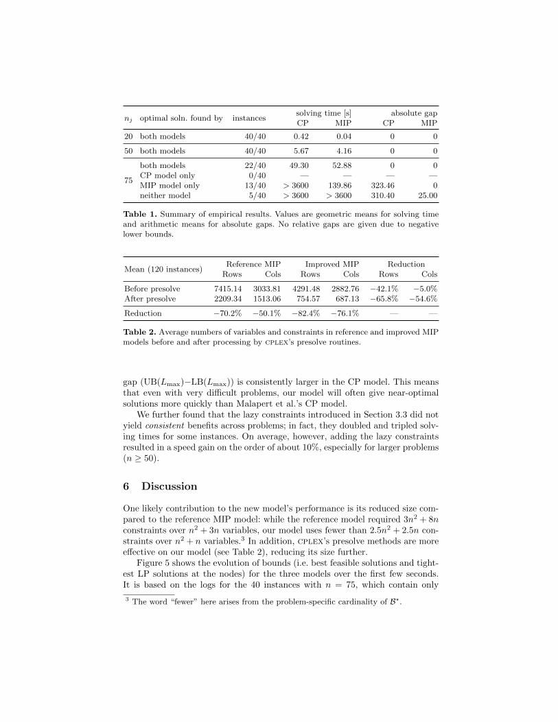
The overview in Table 1 shows aggregated results that demonstrate the perfor-mance and robustness of our new model. As shown in Figure 3, our MIP modelperforms better overall on instances with nj = 20 and nj = 75, while MIP andCP perform similarly well on intermediate problems (nj = 50).

Wherever an optimal solution was not found, the improved MIP modelachieved a significantly better solution quality: out of the 40 instances withnj = 75, 22 were solved to optimality by both CP and MIP, 13 were solvedto optimality by the MIP only, and 5 were solved by neither model within anhour. A comparison of solution quality where no optimal schedule was foundconfirms the robustness of the improved MIP model: as Figure 4 illustrates, the

2 The authors would like to extend a warm thank-you to Arnaud Malapert for bothproviding his code and helping us run it.

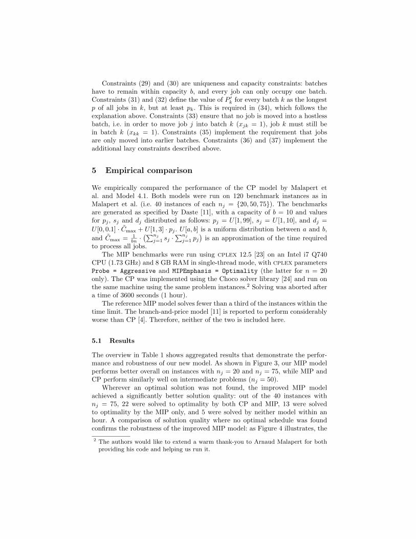
nj optimal soln. found by instancessolving time [s] absolute gapCP MIP CP MIP

20 both models 40/40 0.42 0.04 0 0

50 both models 40/40 5.67 4.16 0 0

75

both models 22/40 49.30 52.88 0 0CP model only 0/40 — — — —MIP model only 13/40 > 3600 139.86 323.46 0neither model 5/40 > 3600 > 3600 310.40 25.00

Table 1. Summary of empirical results. Values are geometric means for solving timeand arithmetic means for absolute gaps. No relative gaps are given due to negativelower bounds.

Mean (120 instances)Reference MIP Improved MIP Reduction

Rows Cols Rows Cols Rows Cols

Before presolve 7415.14 3033.81 4291.48 2882.76 −42.1% −5.0%After presolve 2209.34 1513.06 754.57 687.13 −65.8% −54.6%

Reduction −70.2% −50.1% −82.4% −76.1% — —

Table 2. Average numbers of variables and constraints in reference and improved MIPmodels before and after processing by cplex’s presolve routines.

gap (UB(Lmax)−LB(Lmax)) is consistently larger in the CP model. This meansthat even with very difficult problems, our model will often give near-optimalsolutions more quickly than Malapert et al.’s CP model.

We further found that the lazy constraints introduced in Section 3.3 did notyield consistent benefits across problems; in fact, they doubled and tripled solv-ing times for some instances. On average, however, adding the lazy constraintsresulted in a speed gain on the order of about 10%, especially for larger problems(n ≥ 50).

6 Discussion

One likely contribution to the new model’s performance is its reduced size com-pared to the reference MIP model: while the reference model required 3n2 + 8nconstraints over n2 + 3n variables, our model uses fewer than 2.5n2 + 2.5n con-straints over n2 + n variables.3 In addition, cplex’s presolve methods are moreeffective on our model (see Table 2), reducing its size further.

Figure 5 shows the evolution of bounds (i.e. best feasible solutions and tight-est LP solutions at the nodes) for the three models over the first few seconds.It is based on the logs for the 40 instances with n = 75, which contain only

3 The word “fewer” here arises from the problem-specific cardinality of B?.

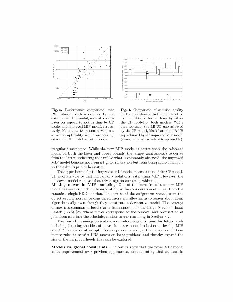
Fig. 3. Performance comparison over120 instances, each represented by onedata point. Horizontal/vertical coordi-nates correspond to solving time by CPmodel and improved MIP model, respec-tively. Note that 18 instances were notsolved to optimality within an hour byeither the CP model or both models.

Fig. 4. Comparison of solution qualityfor the 18 instances that were not solvedto optimality within an hour by eitherthe CP model or both models. Whitebars represent the LB-UB gap achievedby the CP model, black bars the LB-UBgap achieved by the improved MIP model(straight line where solved to optimality).

irregular timestamps. While the new MIP model is better than the referencemodel on both the lower and upper bounds, the largest gain appears to derivefrom the latter, indicating that unlike what is commonly observed, the improvedMIP model benefits not from a tighter relaxation but from being more amenableto the solver’s primal heuristics.

The upper bound for the improved MIP model matches that of the CP model.CP is often able to find high quality solutions faster than MIP. However, theimproved model removes that advantage on our test problems.Making moves in MIP modeling One of the novelties of the new MIPmodel, as well as much of its inspiration, is the consideration of moves from thecanonical single-EDD solution. The effects of the assignment variables on theobjective function can be considered discretely, allowing us to reason about themalgorithmically even though they constitute a declarative model. The conceptof moves is common in local search techniques including Large NeighbourhoodSearch (LNS) [25] where moves correspond to the removal and re-insertion ofjobs from and into the schedule, similar to our reasoning in Section 3.2.

This line of reasoning presents several interesting directions for future workincluding (i) using the idea of moves from a canonical solution to develop MIPand CP models for other optimization problems and (ii) the derivation of dom-inance rules to restrict LNS moves on large problems and thereby expand thesize of the neighbourhoods that can be explored.

Models vs. global constraints Our results show that the novel MIP modelis an improvement over previous approaches, demonstrating that at least in

Fig. 5. Evolution of upper and lower bounds. Left cutoffs indicate the approximatemean time at which the respective bound was first found.

this case, the performance of a specialized global constraint implementation canindeed be matched and exceeded by a comparatively simple mathematical for-mulation. Mathematical models have the general benefit of being more readilyunderstandable, straightforward to implement and reasonably easy to adapt tonew, similar problems.

A global constraint is most valuable when it is the encapsulation of a problemstructure that occurs across a number of interesting problem types. It can thenbe used far beyond its original context. However, with the flexibility to definearbitrary inference operations comes the temptation to develop problem-specificglobal constraints and to trade the ideal of re-usability for problem solving power.We believe that the collection of global constraints in CP is mature enough thatmost problem-specific efforts are now best placed on exploring novel ways toexploit problem structure using existing global constraints. To this end, one ofour current research efforts is the development of a CP model exploiting thepropositions proved in this paper without needing novel global constraints.

7 Conclusion

In this paper, we addressed an existing parallel-batch scheduling problem forwhich CP is the current state-of-the-art approach. Inspired by the idea of movesfrom a canonical solution, we proved a number of propositions allowing us tocreate a novel MIP model that, after presolving, is less than half the size of theprevious MIP model. Empirical results demonstrated that, primarily due to theability to find good feasible solutions quickly, the new MIP model was able toout-perform the existing CP approach over a broad range of problem instancesboth in terms of finding and proving optimality and in terms of finding highquality solutions when the optimal solution could not be proved.

References

[1] Hooker, J.: A hybrid method for planning and scheduling. Constraints 10 (2005)385–401

[2] Beck, J.C., Feng, T.K., Watson, J.P.: Combining constraint programming andlocal search for job-shop scheduling. INFORMS Journal on Computing 23(1)(2011) 1–14

[3] Tran, T.T., Beck, J.C.: Logic-based benders decomposition for alternative re-source scheduling with sequence-dependent setups. In: Proceedings of the Twen-tieth European Conference on Artificial Intelligence (ECAI2012). (2012) 774–779

[4] Malapert, A., Gueret, C., Rousseau, L.M.: A constraint programming approachfor a batch processing problem with non-identical job sizes. European Journal ofOperational Research 221 (2012) 533–545

[5] Schutt, A., Feydy, T., Stuckey, P.J., Wallace, M.: Solving RCPSP/max by lazyclause generation. Journal of Scheduling 16(3) (2013) 273–289

[6] Baptiste, P., Le Pape, C.: Constraint propagation and decomposition techniquesfor highly disjunctive and highly cumulative project scheduling problems. Con-straints 5(1-2) (2000) 119–139

[7] Baptiste, P., Le Pape, C., Nuijten, W.: Constraint-based Scheduling. KluwerAcademic Publishers (2001)

[8] Vilım, P.: Edge finding filtering algorithm for discrete cumulative resources inO(kn log n). In: Principles and Practice of Constraint Programming-CP 2009.Springer (2009) 802–816

[9] Freuder, E.C.: In pursuit of the holy grail. Constraints 2 (1997) 57–61[10] Heinz, S., Ku, W.Y., Beck, J.C.: Recent improvements using constraint integer

programming for resource allocation and scheduling. In Gomes, C., Sellmann, M.,eds.: Integration of AI and OR Techniques in Constraint Programming for Com-binatorial Optimization Problems. Volume 7874 of Lecture Notes in ComputerScience. Springer Berlin Heidelberg (2013) 12–27

[11] Daste, D., Gueret, C., Lahlou, C.: A branch-and-price algorithm to minimize themaximum lateness on a batch processing machine. In: Proceedings of the 11th

International Workshop on Project Management and Scheduling (PMS), Istanbul,Turkey. (2008) 64–69

[12] Lee, C.Y., Uzsoy, R., Martin-Vega, L.A.: Efficient algorithms for scheduling semi-conductor burn-in operations. Oper. Res. 40(4) (July 1992) 764–775

[13] Grossmann, I.E.: Mixed-integer optimization techniques for the design andscheduling of batch processes. Technical Report Paper 203, Carnegie Mellon Uni-versity Engineering Design Research Center and Department of Chemical Engi-neering (1992)

[14] Brucker, P., Gladky, A., Hoogeveen, H., Kovalyov, M.Y., Potts, C.N., Tautenhahn,T., van de Velde, S.L.: Scheduling a batching machine. Journal of Scheduling 1(1)(1998) 31–54

[15] Pinedo, M.L.: Scheduling: Theory, Algorithms, and Systems. 2nd edn. Prentice-Hall (2003)

[16] Shaw, P.: A constraint for bin packing. In Wallace, M., ed.: Proceedings of the 10th

International Conference on Principles and Practice of Constraint Programming(CP 2004). Volume 3258 of Lecture Notes in Computer Science. (2004) 648–662

[17] Azizoglu, M., Webster, S.: Scheduling a batch processing machine with non-identical job sizes. International Journal of Production Research 38(10) (2000)2173–2184

[18] Dupont, L., Dhaenens-Flipo, C.: Minimizing the makespan on a batch machinewith non-identical job sizes: an exact procedure. Computers & Operations Re-search 29(7) (2002) 807–819

[19] Sabouni, M.Y., Jolai, F.: Optimal methods for batch processing problem withmakespan and maximum lateness objectives. Applied Mathematical Modelling34(2) (2010) 314–324

[20] Kashan, A.H., Karimi, B., Ghomi, S.M.T.F.: A note on minimizing makespanon a single batch processing machine with nonidentical job sizes. TheoreticalComputer Science 410(27-29) (2009) 2754–2758

[21] Ozturk, O., Espinouse, M.L., Mascolo, M.D., Gouin, A.: Makespan minimisationon parallel batch processing machines with non-identical job sizes and releasedates. International Journal of Production Research 50(20) (2012) 6022–6035

[22] IBM ILOG: User’s manual for cplex (2013)[23] Ilog, I.: Cplex optimization suite 12.5 (2013)[24] Choco Team: Choco: An open source java constraint programming library. version

2.1.5 (2013)[25] Shaw, P.: Using constraint programming and local search methods to solve vehicle

routing problems. In: Proceedings of the Fourth International Conference onPricinples and Practice of Constraint Programming. Volume 1520 of Lecture Notesin Computer Science. (1998) 417–431