Embed Size (px)
Citation preview
A New Multigrid Method for MolecularMechanics
Pingbing Ming
k [email protected] http//lsec.cc.ac.cn/˜mpb
Joint with Jingrun Chen (ICMSEC)
&W. E (Princeton University)
Supported by 973, NSFC
Ecole des Ponts –Peking University Joint Workshop, 01/04–01/09, 2009
Outline
Motivation and algorithm
Examples
Homogeneous deformation:tension in 1d
tension in Aluminum (3d)
shear in Aluminum
Inhomogeneous deformation:Vacancy (Aluminum)nanoindentation (Aluminum)
Summary
Multigrid Method – p.1
Atomistic model of crystalline solids
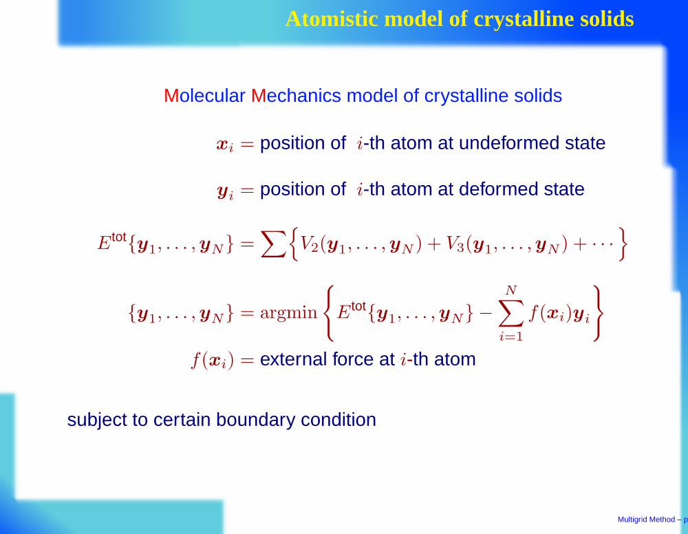
Molecular Mechanics model of crystalline solids
xi = position of i-th atom at undeformed state
yi = position of i-th atom at deformed state
Etoty1, . . . , yN =∑
V2(y1, . . . , yN ) + V3(y1, . . . , yN ) + · · ·
y1, . . . , yN = argmin
Etoty1, . . . , yN −N
∑
i=1
f(xi)yi
f(xi) = external force at i-th atom
subject to certain boundary condition
Multigrid Method – p.2
Difficulty in solving molecular mechanics
Total energy is nonconvex w.r.t. position of atoms; Fortunately, weaim for the physically relevant local minimizer instead of globalminimizer (cf. geometry optimization problem: look for globalminimization configuration)
How to find the physically relevant local minimizer efficiently?
Larger the atomistic system, more the local minimizer
What is a good initial guess for iteration algorithms
Is there any O(N) algorithm=linear scaling algorithm
Multigrid Method – p.3
Local minimizer forest
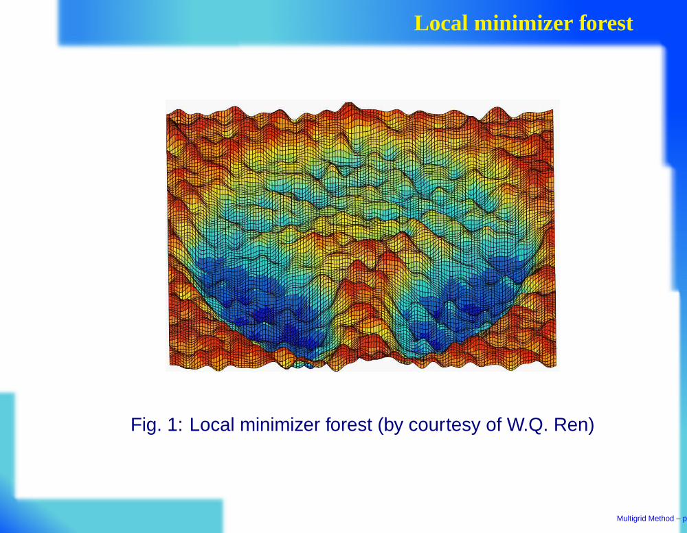
Fig. 1: Local minimizer forest (by courtesy of W.Q. Ren)
Multigrid Method – p.4
Conjugate gradient method is not linear scaling
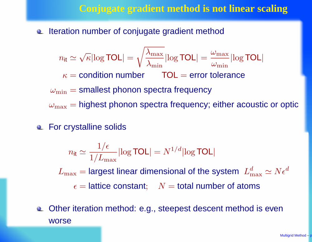
Iteration number of conjugate gradient method
nit ≃√
κ|log TOL| =
√
λmax
λmin
|log TOL| =ωmax
ωmin
|log TOL|
κ = condition number TOL = error tolerance
ωmin = smallest phonon spectra frequency
ωmax = highest phonon spectra frequency; either acoustic or optic
For crystalline solids
nit ≃1/ǫ
1/Lmax
|log TOL| = N1/d|log TOL|
Lmax = largest linear dimensional of the system Ldmax ≃ Nǫd
ǫ = lattice constant; N = total number of atoms
Other iteration method: e.g., steepest descent method is evenworse
Multigrid Method – p.5
Criteria for linear scaling algorithm
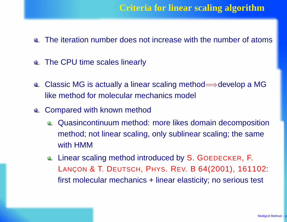
The iteration number does not increase with the number of atoms
The CPU time scales linearly
Classic MG is actually a linear scaling method=⇒develop a MGlike method for molecular mechanics model
Compared with known method
Quasincontinuum method: more likes domain decompositionmethod; not linear scaling, only sublinear scaling; the samewith HMM
Linear scaling method introduced by S. GOEDECKER, F.LANÇON & T. DEUTSCH, PHYS. REV. B 64(2001), 161102:first molecular mechanics + linear elasticity; no serious test
Multigrid Method – p.6
Algorithm
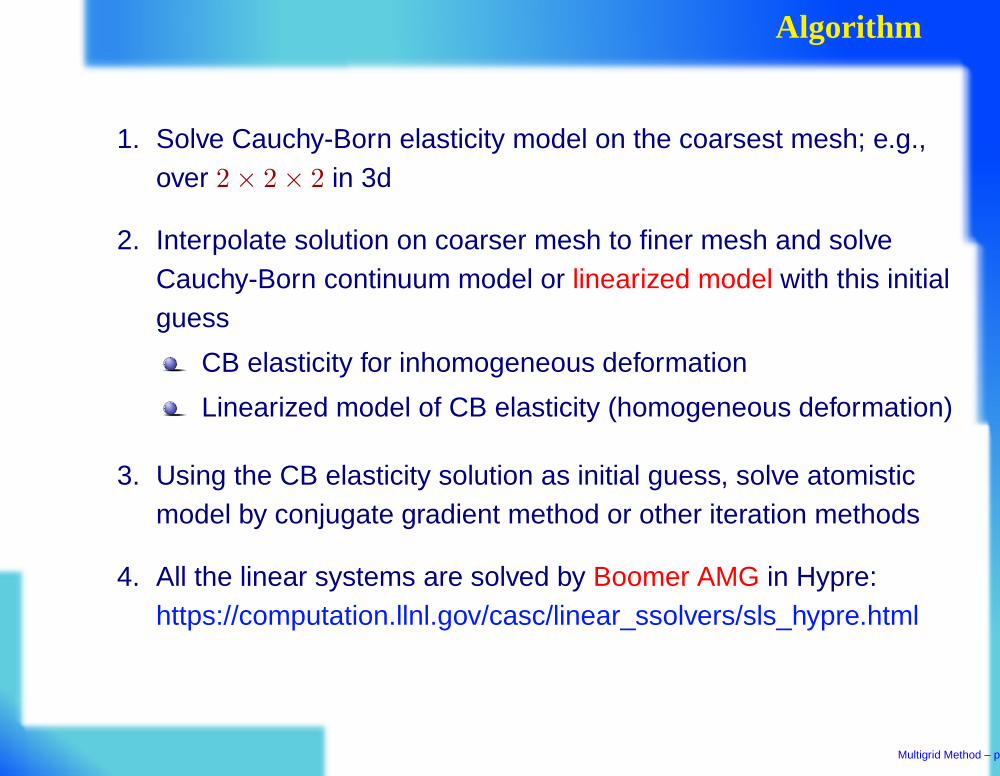
1. Solve Cauchy-Born elasticity model on the coarsest mesh; e.g.,over 2 × 2 × 2 in 3d
2. Interpolate solution on coarser mesh to finer mesh and solveCauchy-Born continuum model or linearized model with this initialguess
CB elasticity for inhomogeneous deformation
Linearized model of CB elasticity (homogeneous deformation)
3. Using the CB elasticity solution as initial guess, solve atomisticmodel by conjugate gradient method or other iteration methods
4. All the linear systems are solved by Boomer AMG in Hypre:https://computation.llnl.gov/casc/linear_ssolvers/sls_hypre.html
Multigrid Method – p.7
Continuum model of solids
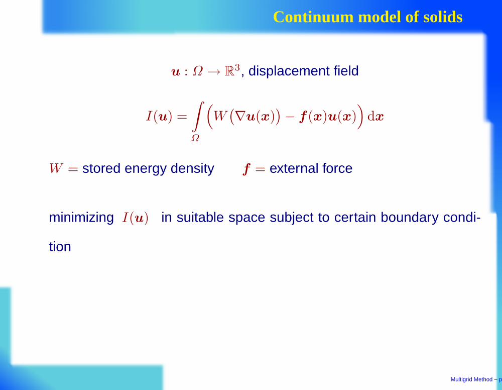
u : Ω → R3, displacement field
I(u) =
∫
Ω
(
W(
∇u(x))
− f(x)u(x))
dx
W = stored energy density f = external force
minimizing I(u) in suitable space subject to certain boundary condi-
tion
Multigrid Method – p.8
Cauchy-Born rule: simple lattice
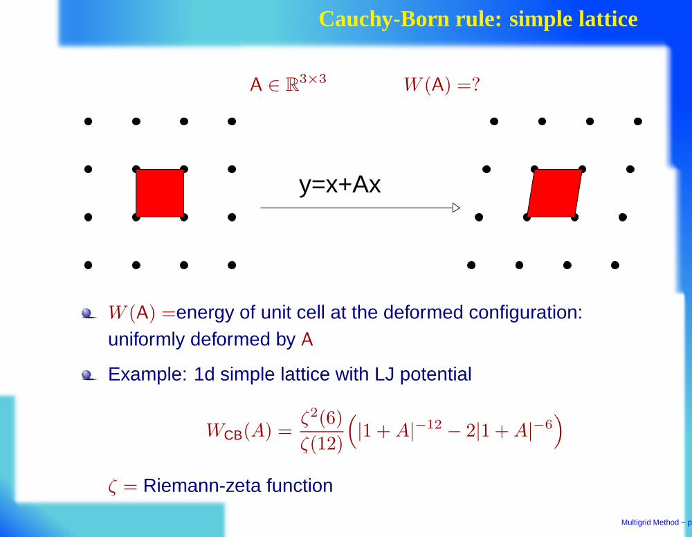
A ∈ R3×3 W (A) =?
y=x+Ax
W (A) =energy of unit cell at the deformed configuration:uniformly deformed by A
Example: 1d simple lattice with LJ potential
WCB(A) =ζ2(6)
ζ(12)
(
|1 + A|−12 − 2|1 + A|−6
)
ζ = Riemann-zeta function
Multigrid Method – p.9
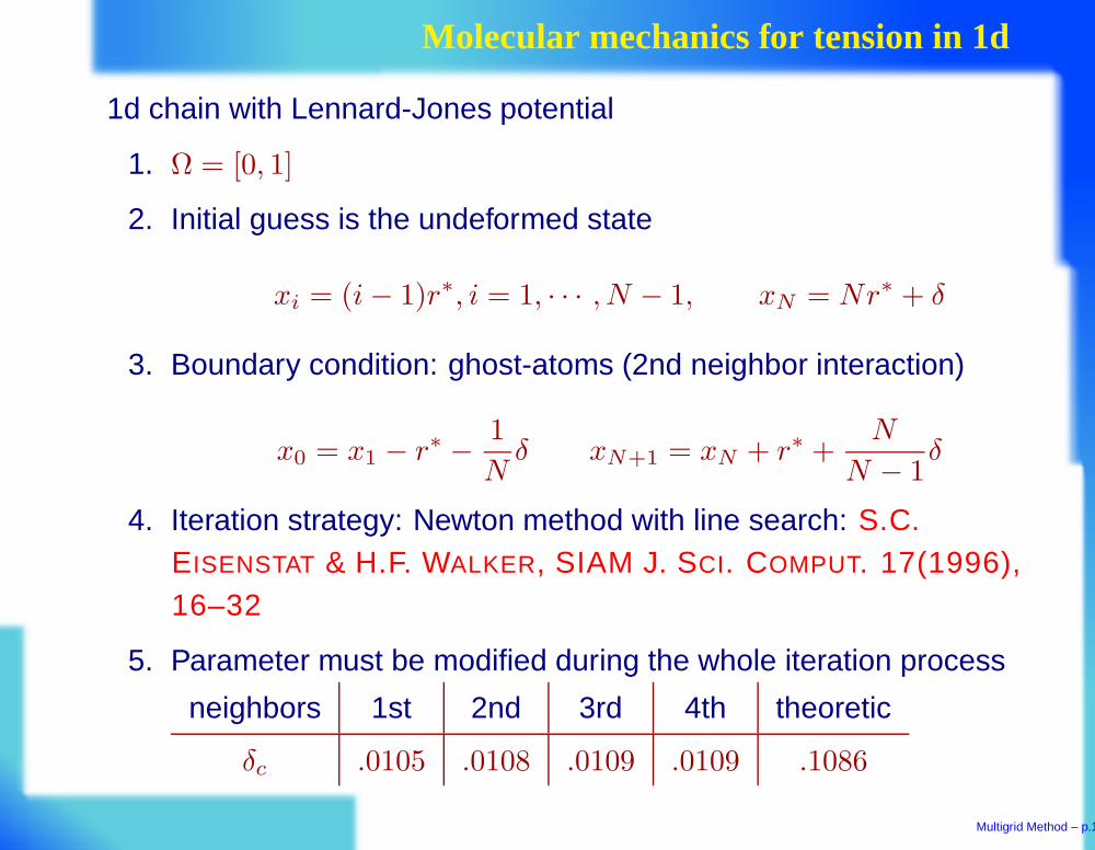
Molecular mechanics for tension in 1d
1d chain with Lennard-Jones potential
1. Ω = [0, 1]
2. Initial guess is the undeformed state
xi = (i − 1)r∗, i = 1, · · · , N − 1, xN = Nr∗ + δ
3. Boundary condition: ghost-atoms (2nd neighbor interaction)
x0 = x1 − r∗ − 1
Nδ xN+1 = xN + r∗ +
N
N − 1δ
4. Iteration strategy: Newton method with line search: S.C.EISENSTAT & H.F. WALKER, SIAM J. SCI. COMPUT. 17(1996),16–32
5. Parameter must be modified during the whole iteration process
neighbors 1st 2nd 3rd 4th theoretic
δc .0105 .0108 .0109 .0109 .1086
Multigrid Method – p.10
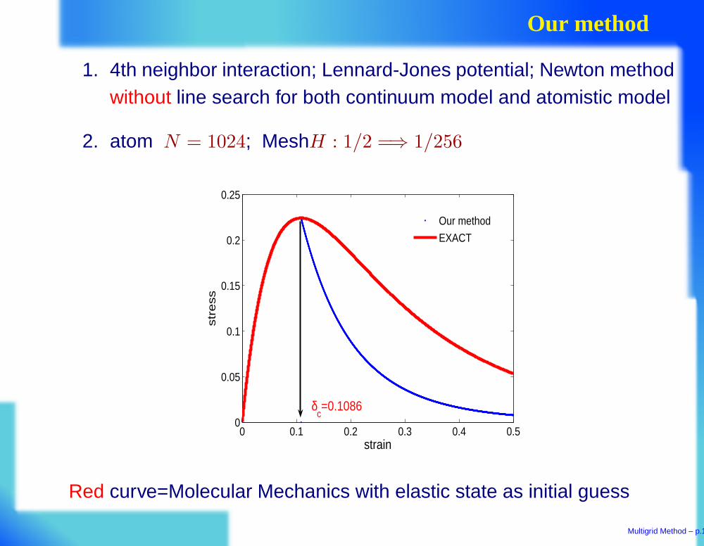
Our method
1. 4th neighbor interaction; Lennard-Jones potential; Newton methodwithout line search for both continuum model and atomistic model
2. atom N = 1024; MeshH : 1/2 =⇒ 1/256
0 0.1 0.2 0.3 0.4 0.50
0.05
0.1
0.15
0.2
0.25
strain
str
ess
Our method
EXACT
δc=0.1086
Red curve=Molecular Mechanics with elastic state as initial guess
Multigrid Method – p.11
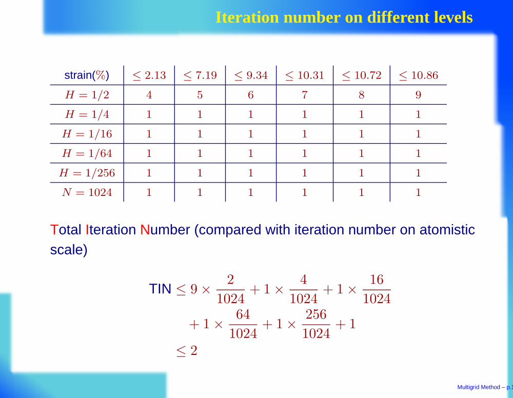
Iteration number on different levels
strain(%) ≤ 2.13 ≤ 7.19 ≤ 9.34 ≤ 10.31 ≤ 10.72 ≤ 10.86
H = 1/2 4 5 6 7 8 9
H = 1/4 1 1 1 1 1 1
H = 1/16 1 1 1 1 1 1
H = 1/64 1 1 1 1 1 1
H = 1/256 1 1 1 1 1 1
N = 1024 1 1 1 1 1 1
Total Iteration Number (compared with iteration number on atomisticscale)
TIN ≤ 9 × 2
1024+ 1 × 4
1024+ 1 × 16
1024
+ 1 × 64
1024+ 1 × 256
1024+ 1
≤ 2
Multigrid Method – p.12
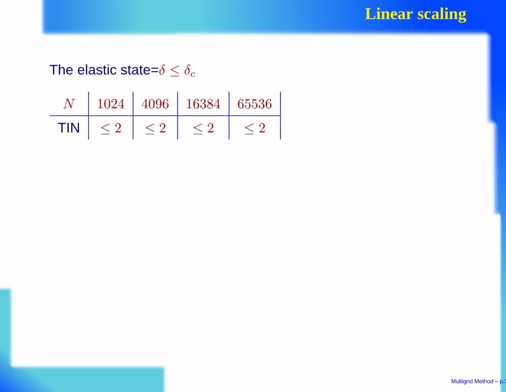
Linear scaling
The elastic state=δ ≤ δc
N 1024 4096 16384 65536
TIN ≤ 2 ≤ 2 ≤ 2 ≤ 2
Multigrid Method – p.13
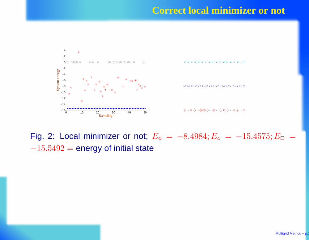
Correct local minimizer or not
0 10 20 30 40 50−16
−14
−12
−10
−8
−6
−4
−2
0
2
4
Sampling
Sys
tem
ene
rgy
Fig. 2: Local minimizer or not; E⋄ = −8.4984; E = −15.4575; E2 =
−15.5492 = energy of initial state
Multigrid Method – p.14
3d: Aluminum
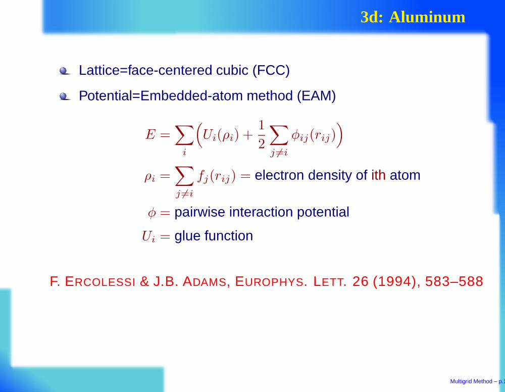
Lattice=face-centered cubic (FCC)
Potential=Embedded-atom method (EAM)
E =∑
i
(
Ui(ρi) +1
2
∑
j 6=i
φij(rij))
ρi =∑
j 6=i
fj(rij) = electron density of ith atom
φ = pairwise interaction potential
Ui = glue function
F. ERCOLESSI & J.B. ADAMS, EUROPHYS. LETT. 26 (1994), 583–588
Multigrid Method – p.15
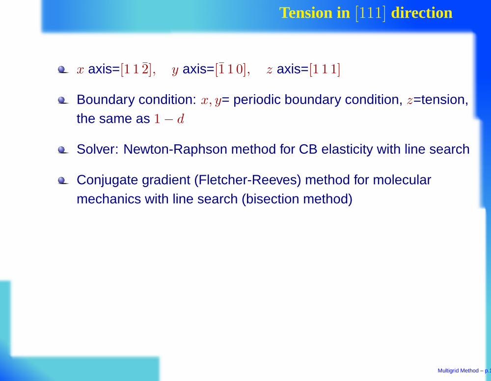
Tension in [111] direction
x axis=[1 1 2], y axis=[1 1 0], z axis=[1 1 1]
Boundary condition: x, y= periodic boundary condition, z=tension,the same as 1 − d
Solver: Newton-Raphson method for CB elasticity with line search
Conjugate gradient (Fletcher-Reeves) method for molecularmechanics with line search (bisection method)
Multigrid Method – p.16
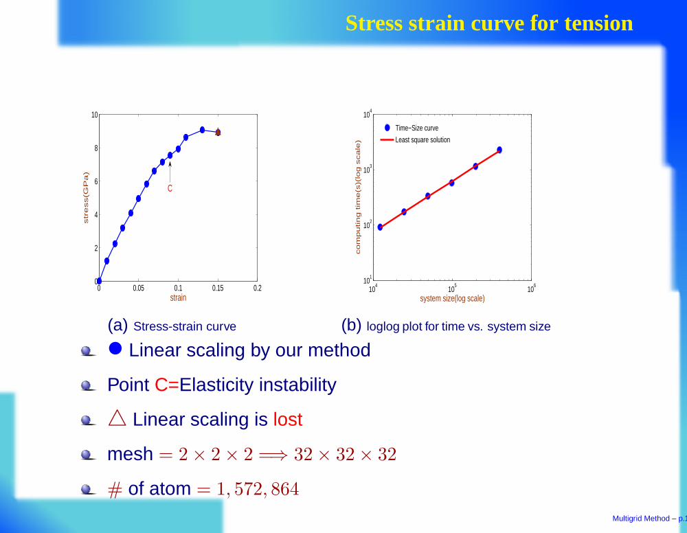
Stress strain curve for tension
0 0.05 0.1 0.15 0.20
2
4
6
8
10
strain
str
ess(G
Pa
)
C
(a) Stress-strain curve
104
105
106
101
102
103
104
system size(log scale)
co
mp
utin
g tim
e(s
)(lo
g s
ca
le)
Time−Size curve
Least square solution
(b) loglog plot for time vs. system size
• Linear scaling by our method
Point C=Elasticity instability
Linear scaling is lost
mesh = 2 × 2 × 2 =⇒ 32 × 32 × 32
# of atom = 1, 572, 864
Multigrid Method – p.17
Linear scaling
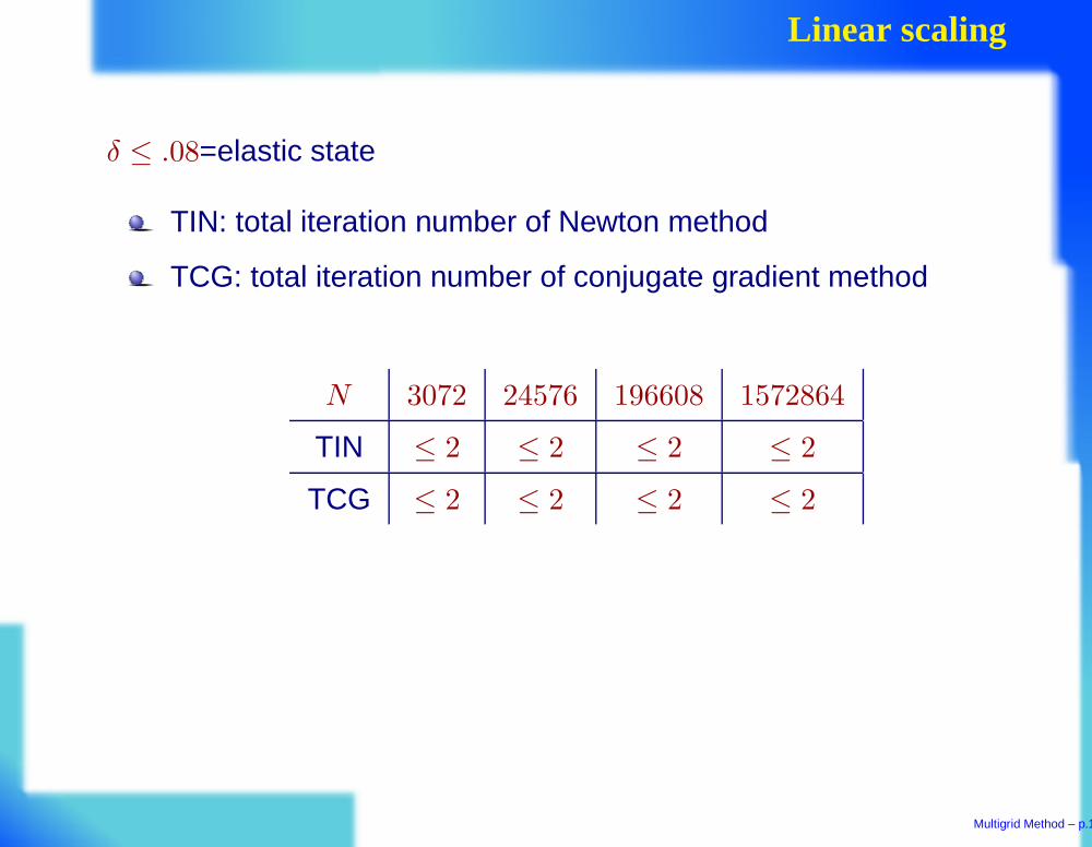
δ ≤ .08=elastic state
TIN: total iteration number of Newton method
TCG: total iteration number of conjugate gradient method
N 3072 24576 196608 1572864
TIN ≤ 2 ≤ 2 ≤ 2 ≤ 2
TCG ≤ 2 ≤ 2 ≤ 2 ≤ 2
Multigrid Method – p.18
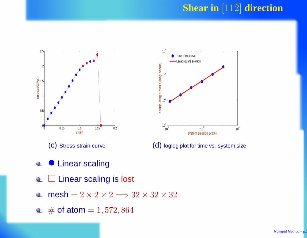
Shear in [112] direction
0 0.05 0.1 0.15 0.20
0.5
1
1.5
2
2.5
strain
str
ess(G
Pa
)
(c) Stress-strain curve
104
105
106
101
102
103
104
system size(log scale)
co
mp
utin
g tim
e(s
)(lo
g s
ca
le)
Time−Size curve
Least square solution
(d) loglog plot for time vs. system size
• Linear scaling
Linear scaling is lost
mesh = 2 × 2 × 2 =⇒ 32 × 32 × 32
# of atom = 1, 572, 864
Multigrid Method – p.19
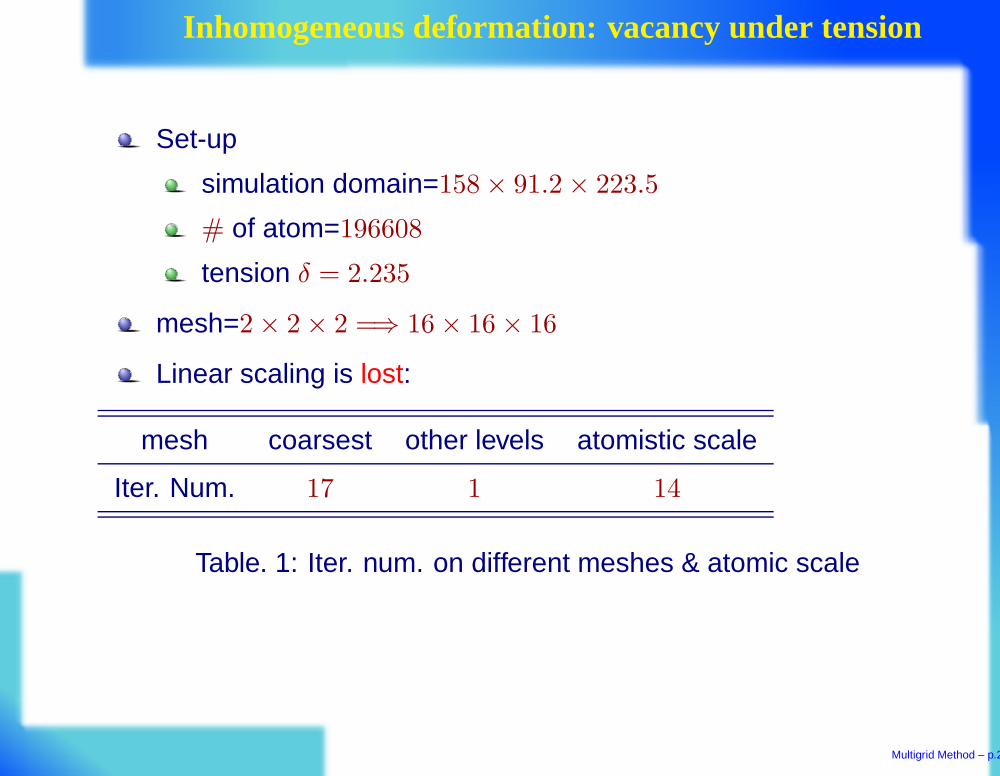
Inhomogeneous deformation: vacancy under tension
Set-up
simulation domain=158 × 91.2 × 223.5
# of atom=196608
tension δ = 2.235
mesh=2 × 2 × 2 =⇒ 16 × 16 × 16
Linear scaling is lost:
mesh coarsest other levels atomistic scale
Iter. Num. 17 1 14
Table. 1: Iter. num. on different meshes & atomic scale
Multigrid Method – p.20
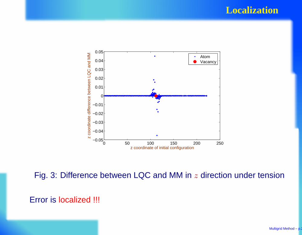
Localization
0 50 100 150 200 250−0.05
−0.04
−0.03
−0.02
−0.01
0
0.01
0.02
0.03
0.04
0.05
z coordinate of initial configuration
z co
ordi
nate
diff
eren
ce b
etw
een
LQC
and
MM Atom
Vacancy
Fig. 3: Difference between LQC and MM in z direction under tension
Error is localized !!!
Multigrid Method – p.21
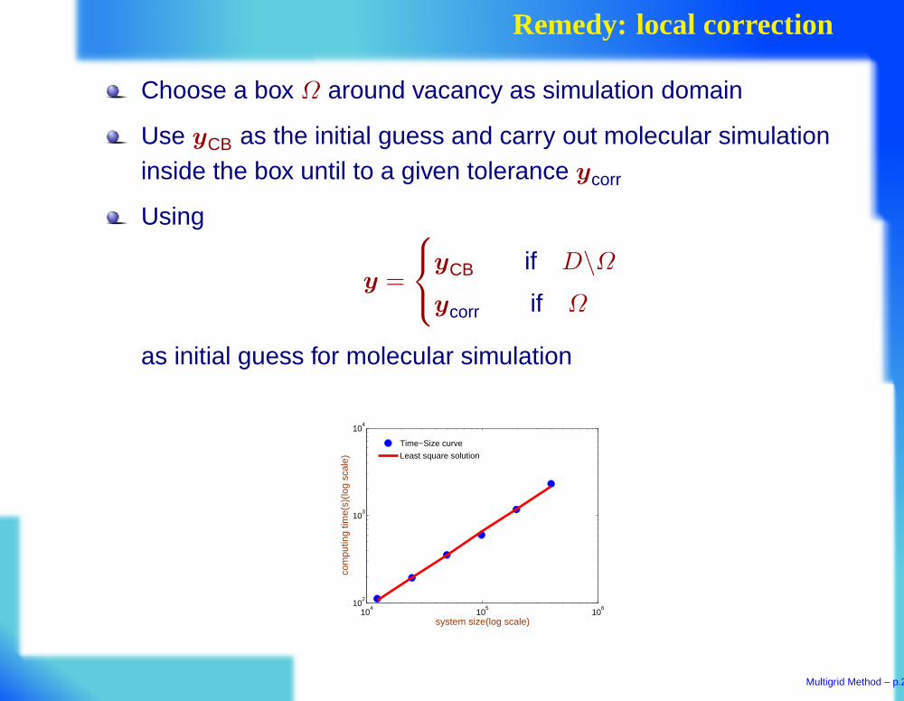
Remedy: local correction
Choose a box Ω around vacancy as simulation domain
Use yCB as the initial guess and carry out molecular simulationinside the box until to a given tolerance ycorr
Using
y =
yCB if D\Ωycorr if Ω
as initial guess for molecular simulation
104
105
106
102
103
104
system size(log scale)
com
putin
g tim
e(s)
(log
scal
e)
Time−Size curve
Least square solution
Multigrid Method – p.22
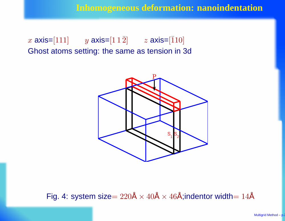
Inhomogeneous deformation: nanoindentation
x axis=[111] y axis=[1 1 2] z axis=[110]
Ghost atoms setting: the same as tension in 3d
S1
S2
P
Fig. 4: system size= 220Å × 40Å × 46Å;indentor width= 14Å
Multigrid Method – p.23
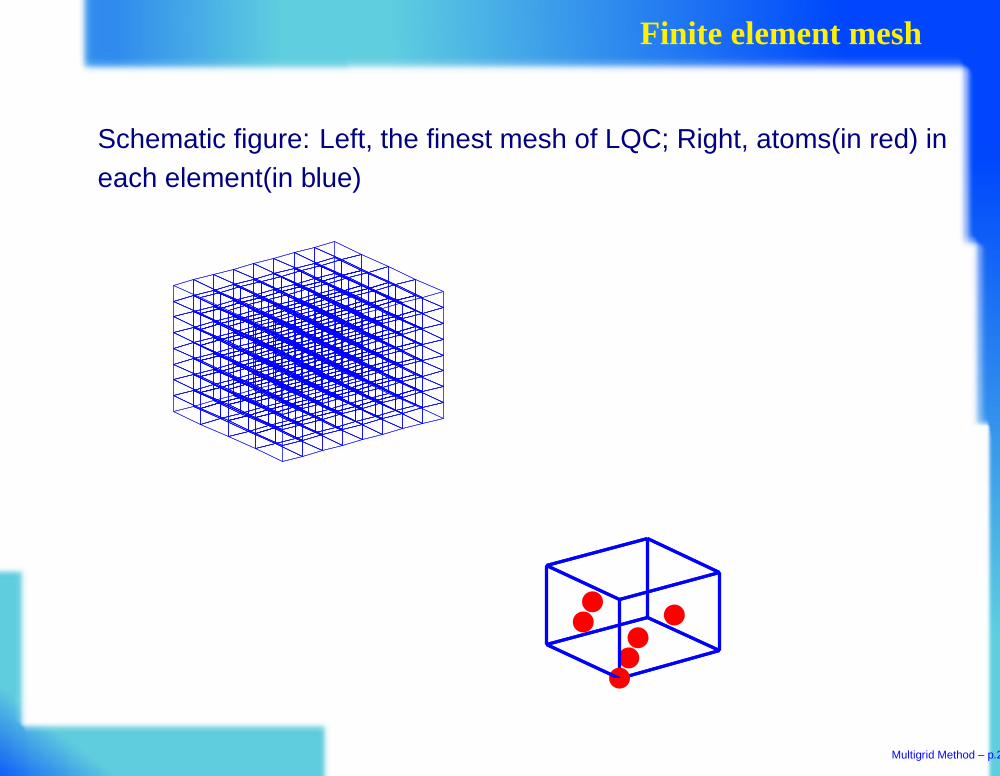
Finite element mesh
Schematic figure: Left, the finest mesh of LQC; Right, atoms(in red) ineach element(in blue)
Multigrid Method – p.24
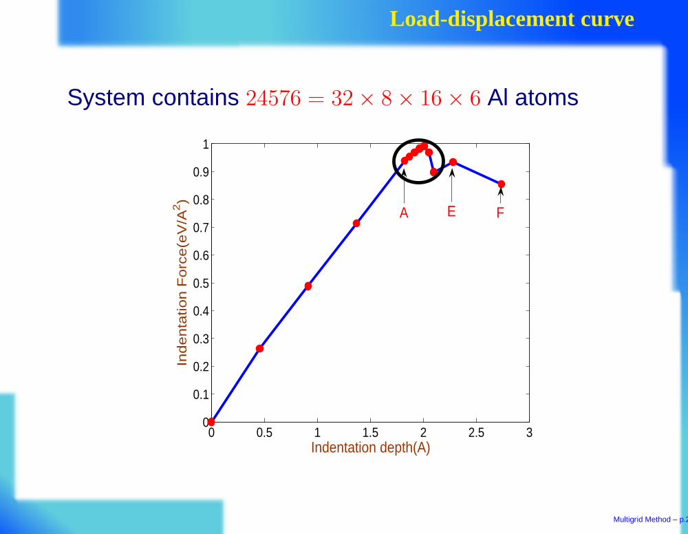
Load-displacement curve
System contains 24576 = 32 × 8 × 16 × 6 Al atoms
0 0.5 1 1.5 2 2.5 30
0.1
0.2
0.3
0.4
0.5
0.6
0.7
0.8
0.9
1
Indentation depth(A)
Ind
en
tatio
n F
orc
e(e
V/A
2)
A E F
Multigrid Method – p.25
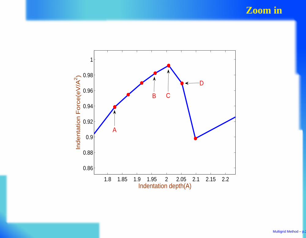
Zoom in
1.8 1.85 1.9 1.95 2 2.05 2.1 2.15 2.2
0.86
0.88
0.9
0.92
0.94
0.96
0.98
1
Indentation depth(A)
Ind
en
tatio
n F
orc
e(e
V/A
2)
A
B C
D
Multigrid Method – p.26
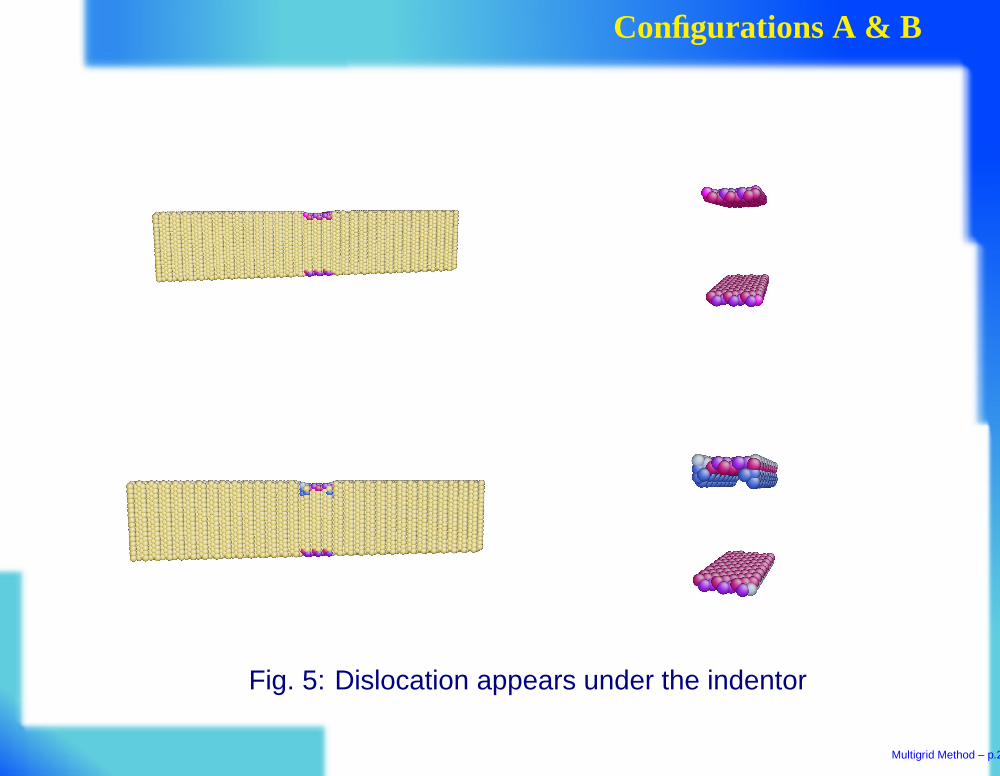
Configurations A & B
Fig. 5: Dislocation appears under the indentor
Multigrid Method – p.27
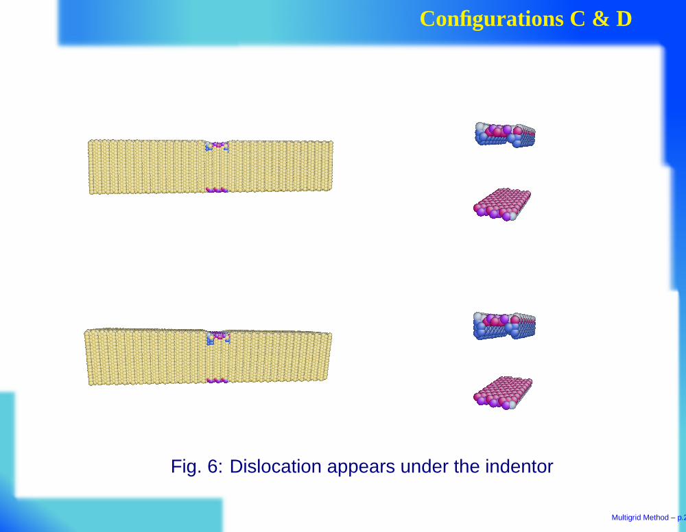
Configurations C & D
Fig. 6: Dislocation appears under the indentor
Multigrid Method – p.28
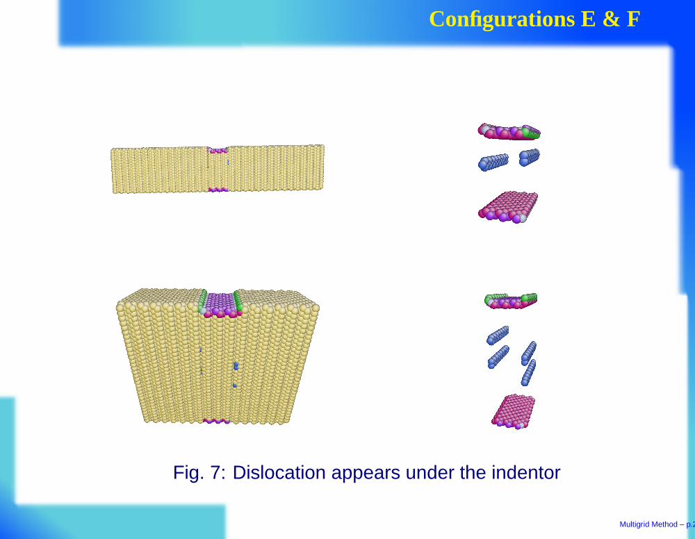
Configurations E & F
Fig. 7: Dislocation appears under the indentor
Multigrid Method – p.29
Discussion
Results
Dislocation (B) comes in before the load-displacement curvedecreases(dC)
Plasticity cannot be judged by load-displacement curve
Although the system is small, above results are conforming with with
Numerical result: number of atom= 2.5 × 10¹¹: (J. KNAP AND M.ORTIZ, PHYS. REV. LETT. 90 (2003) , 226102)
Experiment result: (A.M. MINOR, S.A. SYED ASIF , Z.W. SHAN,E.A. STACH, E. CYRANKOWSKI, T.J. WYROBEK & O.L. WARREN,NATURE MATERIALS 5 (2006), 697-702))
Multigrid Method – p.30
Iteration numbers
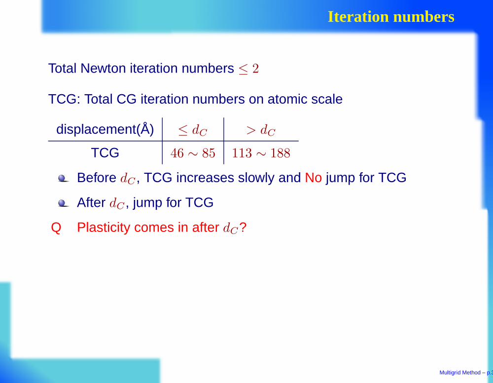
Total Newton iteration numbers ≤ 2
TCG: Total CG iteration numbers on atomic scale
displacement(Å) ≤ dC > dC
TCG 46 ∼ 85 113 ∼ 188
Before dC , TCG increases slowly and No jump for TCG
After dC , jump for TCG
Q Plasticity comes in after dC?
Multigrid Method – p.31
Two stability regions
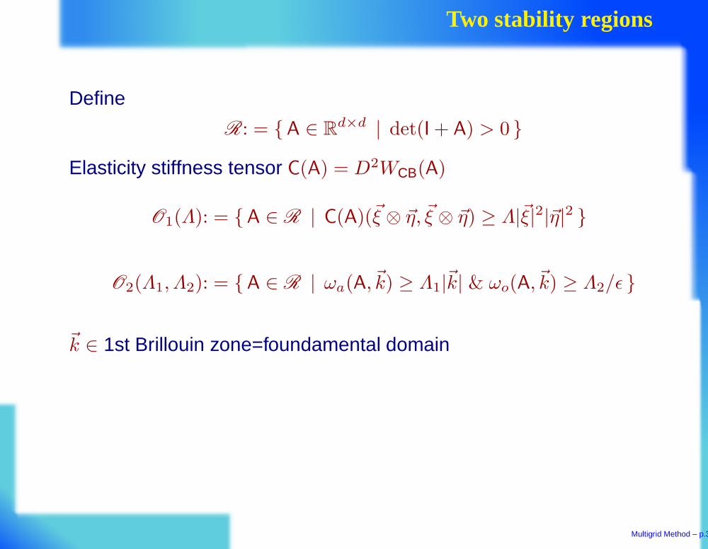
Define
R: = A ∈ Rd×d | det(I + A) > 0
Elasticity stiffness tensor C(A) = D2WCB(A)
O1(Λ): = A ∈ R | C(A)(~ξ ⊗ ~η, ~ξ ⊗ ~η) ≥ Λ|~ξ|2|~η|2
O2(Λ1, Λ2): = A ∈ R | ωa(A, ~k) ≥ Λ1|~k| & ωo(A, ~k) ≥ Λ2/ǫ
~k ∈ 1st Brillouin zone=foundamental domain
Multigrid Method – p.32
Theoretical result[E–M, ARMA, 07]
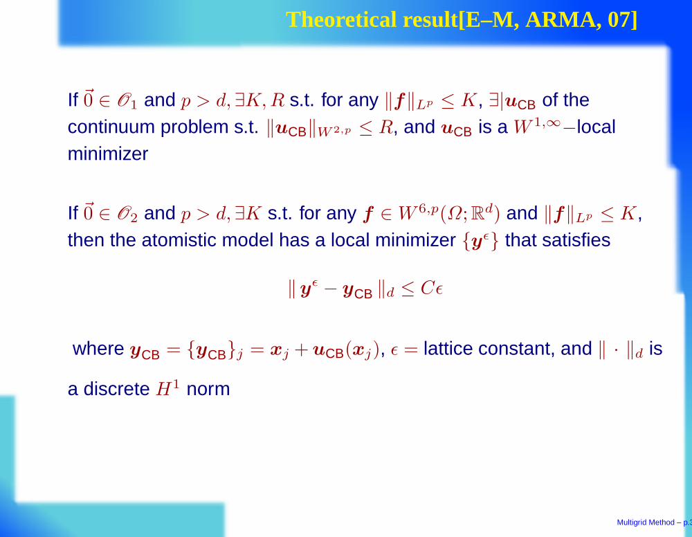
If ~0 ∈ O1 and p > d, ∃K, R s.t. for any ‖f‖Lp ≤ K, ∃|uCB of thecontinuum problem s.t. ‖uCB‖W 2,p ≤ R, and uCB is a W 1,∞−localminimizer
If ~0 ∈ O2 and p > d, ∃K s.t. for any f ∈ W 6,p(Ω; Rd) and ‖f‖Lp ≤ K,then the atomistic model has a local minimizer yǫ that satisfies
‖yǫ − yCB ‖d ≤ Cǫ
where yCB = yCBj = xj + uCB(xj), ǫ = lattice constant, and ‖ · ‖d is
a discrete H1 norm
Multigrid Method – p.33
Summary of Our method
In elastic regime
Physically reasonable configuration
Insensitive to parameters of nonlinear iteration method
Linear scaling of the computing complexity
Linear scaling is recovered if local correction is added(Vacancy)
Out of this regime
Physical reasonable result (nanoindentation)
unphysical configuration (tension)
Linear scaling is lost (tension, nanoindentation)
An efficient way to find physically relevant local minimizer; Hiddenmechanism: automatically bypass many unphysically localminimizer
Multigrid Method – p.34
Conclusion
Drawbacks of the algorithm:
Inefficient for inhomogeneous deformation
Adaptive FEM is required in solving Cauchy-Born elasticity
More realistic applications are needed: e.g., othernanoindentation simulation; dislocation/fracture (Maradudin,Tewary)
Theoretically understand of this alg., e.g.,
Mechanism for bypassing local minimizer
Rigorous prove the algorithm is linear scaling, at least forhomogeneous deformation; vacancy is much harder
Multigrid Method – p.35
Extension and perspective
Wider implementation: lattice equations in many other fields
Repetitive structure in solid mechanics (A.K. Noor)
Power grid (Babuska, Sauter)
Protein folding lattice model (Thumas, 1995)
Ising model
Quantum chromodynamics (lattice QCD)
Integer programming problem in operations research
Lattice-based cryptography and communication theory
Difficulty
Do all the aforementioned problems concern local minima
Does there exists an efficient macroscopic model as CBelasticity in crystalline solids (e.g., finite differencehomogenization for linear lattice equation)
Multigrid Method – p.36