WP/06/105

A New Risk Indicator and Stress Testing Tool: A Multifactor Nth-to-Default CDS Basket

Renzo G. Avesani, Antonio García Pascual,

and Jing Li

© 2006 International Monetary Fund WP/06/105

IMF Working Paper

Monetary and Financial Systems Department

A New Risk Indicator and Stress Testing Tool: A Multifactor Nth-to-Default CDS Basket

Prepared by Renzo G. Avesani, Antonio García Pascual, and Jing Li1

Authorized for distribution by David Marston

April 2006

Abstract

This Working Paper should not be reported as representing the views of the IMF. The views expressed in this Working Paper are those of the author(s) and do not necessarily represent those of the IMF or IMF policy. Working Papers describe research in progress by the author(s) and are published to elicit comments and to further debate.

This paper generalizes a market-based indicator for financial sector surveillance using a multifactor latent structure in the determination of the default probabilities of an nth-to-default credit default swap (CDS) basket of large complex financial institutions (LCFIs). To estimate the multifactor latent structure, we link the market risk (the covariance of the LCFIs’ equity) to credit risk (the default probability of the CDS basket) in a coherent manner. In addition, to analyze the response of the probabilities of default to changing macroeconomic conditions, we run a stress test by generating shocks to the latent multifactor structure. The results unveil a rich set of default probability dynamics and help in identifying the most relevant sources of risk. We anticipate that this approach could be of value to financial supervisors and risk managers alike. JEL Classification Numbers: G11, G13, G15, G21, G24 Keywords: Risk management, market indicators, stress testing, credit default swap (CDS),

collateralized debt obligation (CDO), credit risk, large complex financial institutions (LCFIs)

Author(s) E-Mail Address: ravesani@imf.org; agarciapascual@imf.org; jli2@imf.org

1 We would like to thank Gianni De Nicolo, Mike Gibson, Eduardo Ley, David Marston, Salih Neftci, Fabio Stella, Walter Vecchiato, and seminar participants at the Research Department of the IMF for comments. Special thanks go to Kexue Liu for his valuable help with the programming.

- 2 -

Contents Page

I. Introduction ............................................................................................................................3

II. Description of the Indicator...................................................................................................4

III. Model Description ...............................................................................................................5

IV. Data Description ..................................................................................................................7

V. Factor ANALYSIS: Estimation Results ..............................................................................9

VI. Computation of the Probabilities of Default......................................................................12

VII. Sensitivity Analysis..........................................................................................................15

VIII. Stress Testing .................................................................................................................18

IX. Concluding Remarks ........................................................................................................21 References................................................................................................................................22 Tables 1. Large Complex Financial Institutions: Estimated Correlations.............................................9 2. Rotated Factor Loadings, Maximum Likelihood Estimates ................................................11 3. Variance Contribution..........................................................................................................12 Figures 1. Large Complex Financial Institutions: Credit Spreads..........................................................8 2. Probability of Default: One- to Twenty-Quarter Ahead ......................................................13 3. Two-Year-Ahead Probability of No Defaults......................................................................14 4. Estimated Correlation and Factor Structure (2001-05)........................................................15 5. Default Probabilities under High and Low Correlation Scenarios ......................................16 6. Probability of default over range of correlation and factor structures .................................17 7. Two-year Ahead Probability of Default: Variable vs. Fixed Correlation and Factors ........17 8. Stress Testing: Probabilities of Default Under an All Factor Recession Scenario ..............19 9. Stress Testing: Probabilities of Default under Alternative Recession Scenarios ................20

- 3 -

I. INTRODUCTION

The costly financial crises of the 1990s sparked the interest of supervisory agencies and central banks in developing a broader understanding of financial markets and institutions through macro-prudential analysis. Such analysis is intended to complement the micro analysis of individual institutions, as it aims at unveiling aggregate risks emerging from common shocks and risk correlations across institutions (Crocket, 2000). Large complex financial institutions (LCFIs) play a key role in the stability of global financial markets, and, as such, their surveillance has features of both micro- and macro-prudential analysis. The health of LCFIs can be analyzed by looking at levels and trends in financial soundness indicators, also referred to as macro-prudential indicators. Financial soundness indicators are based on balance sheet information usually published quarterly, semi-annually, or annually.2 A problem with these indicators is their use of lagged, historical information based on balance sheet items, which represent a decreasing proportion of LCFIs activities. To analyze forward-looking information, prices of debt, equity, and derivatives have been proposed in devising early warning indicators of bank performance. One of the most widely used market-based indicators is distance-to-default, which is based on Merton’s seminal contribution (Merton, 1974). Other market measures are based on spreads on (primary and secondary market) subordinated debt issued by banks.3 A problem with the distance-to-default indicators is that they also need some information on balance sheet items and, therefore, they only partially reflect current market information. Additionally, the information content of secondary markets on senior- and subordinated-debt spreads is also hampered by insufficient liquidity in bank bond markets. For these reasons, such indicators have a limited role as timely early warning measures of risks and vulnerabilities emerging in financial institutions. This paper develops a market-based indicator for financial sector surveillance using a basket of credit default swaps (CDSs). It generalizes the approach taken in Avesani (2005) in two main directions. First, it determines and analyzes the multivariate latent factor structure which underpins the LCFIs’ correlation dynamics. By doing so, we move from a framework in which the risk factor sensitivities are the same across institutions and regions, as in the capital asset pricing model (CAPM), to one in which the multifactor risk sensitivities are institution-specific, as in the arbitrage pricing theory (APT).4 Second, it uses the identified 2 The International Monetary Fund (2003) has developed a core set of financial soundness indicators covering the financial sector.

3 See, among others, Flannery and Sorescu (1996) and, more recently, Gropp, Vesala, and Vulpes (2002).

4 See Berndt and others (2005) for an alternative approach to model firm-specific sensitivities to risk factors.

- 4 -

latent factor structure for conducting stress tests in a coherent fashion. Specifically, the risk profile of each institution and of the entire group of LCFIs is stressed through shocks applied to the default correlations and to the values of the identified factors. The paper is organized as follows. The next section provides a description of the market-based indicator. Section III briefly describes the methodology for computing the probabilities of default of a CDS basket in a multifactor framework. This section also presents the econometric estimation of the latent factor structure through factor analysis. Section IV describes the CDS spread data and Section V shows the results of the factor analysis estimation. Section VI shows the results of the computation of the default probabilities for different horizons. Sections VII and VIII contain the sensitivity analysis and stress testing of the probabilities of default to shocks in the correlation and factor structures. Section IX concludes.

II. DESCRIPTION OF THE INDICATOR

Many studies on macro-prudential analysis have been based on the lessons learned from the banking crises of the 1980s and 1990s. In this paper we take a more financial-oriented approach by focusing on the information content, relevant for financial stability analysis, of an nth-to-default CDS basket.5 An nth -to-default CDS basket is the simplest example of a collateralized debt obligation (CDO). A CDO is the securitization of a pool of debt obligations, generally corporate debt, into classes (i.e., the “tranches”) of securities with various levels of exposure to the underlying credit risk. The CDO exposure to the underlying pool of debt securities can be direct, that is, a cash transaction where the CDO owns the actual debt securities (cash CDO), or indirect, that is, a synthetic transaction where the CDO writes CDSs on a pool of corporate names or asset backed securities (synthetic CDO). In a synthetic CDO, the reference portfolio is made up of credit default swaps (CDSs). Much of the risk transfer that occurs in the credit derivatives market is in the form of synthetic CDOs. Understanding the risk characteristics of synthetic CDOs is important for understanding the nature and magnitude of credit risk transfer. In this paper, the synthetic CDO is composed by the actively traded CDSs of 15 large complex financial institutions (LCFIs). The main differences between an nth-to-default basket of CDSs and a CDO are the leverage and exposure, which the CDO provides and the CDSs don’t. The buyer of a CDO (investor) is exposed to the risk caused by the different credit events, which affect the tranches at different points in time. The seller of protection (investor) on an nth -to-default basket of CDSs is exposed only until the specific event on which protection has been sold takes place. For example, in a first-to-default basket, protection on the basket is provided and paid for 5 CDSs are financial contracts where the financial guarantor agrees to make a payment, sometimes subject to a loss threshold, contingent on a credit event concerning the reference asset in exchange for a periodic fee.

- 5 -

only until the first name in the basket is subject to a credit event. After that, the financial instrument ceases to exist. In this sense, a first-to-default basket is similar to the equity tranche of a CDO. Default correlations are the main driver of the CDS basket’s value. Let us suppose that we have a basket of five credits where each CDS pays a spread of 100 basis points (bps). In the case of zero correlation, the first-to-default swap would have a spread of 500 bps, i.e., the simple sum of the individual credit spreads. If, instead, the correlation is one, the spread for the basket would be 100 bps, i.e., the maximum of the individual swap spread. Given the relevance of default correlations, this paper concentrates on the determinants of the default correlation structure underlying an nth -to-default basket of CDSs.

III. MODEL DESCRIPTION

Our modeling strategy is based on two key elements. First, following Hull and White (2005), Gibson (2004), and Andersen, Sidenius, and Basu (2003), we compute the probabilities of default conditional on a multifactor structure. Second, the multifactor structure is estimated by factor analysis and will allow us to express the LCFI’s correlation structure in terms of a set of common factors related to the macroeconomic conditions in which financial institutions operate. As a by-product, the multifactor structure also serves as a platform to conduct stress testing of the default probabilities to shocks in all or some of these factors. The Pricing Model This section presents a schematic representation of the multifactor pricing model. In pricing a CDO or a CDS basket, it is assumed, following Vasicek (1987) and Merton (1974), that the asset value of each institution in the portfolio is influenced by a common set of factors and a specific, idiosyncratic factor. When the value of the asset falls below a certain pre-specified level given by the value of the debt of that institution, the institution defaults. The asset value of financial institution i can be expressed as a random variable )1( Nixi ≤≤ ,

222

212211 ...1... imiiimimiii aaaZMaMaMax −−−−++++= (1)

where the common factors Μ = ( 1M ,…, mM ) and the idiosyncratic factor iZ have independent zero-mean and unit-variance distributions. The factor loadings ija are such that

}1,1{−∈ija and 2 2 21 2 ... 1i i ima a a+ + + ≤ . The correlation matrix among the N institutions,Σ , is

such that the pair-wise correlation between asset i and j can be expressed as jmimjiji aaaaaa +++ ...2211 .

Let H be the cumulative distribution of the iZ . The default probability of ix , i.e., the probability of ix falling below a threshold ix , is characterized as:

- 6 -

1 12 21

( ... )Pr ( | ) ( | )1 ...

i i im mi i i

i im

x a M a Mob x x Q t Ha a

⎡ ⎤− + +⎢ ⎥< Μ = Μ =⎢ ⎥− − −⎣ ⎦

(2)

Let ( , | ),Np l t Μ Nl ,...,0= , denote the probability that exactly l defaults occur by time t , conditional on the common factorsΜ , in a reference portfolio of N financial institutions. Let iF be the cumulative distribution of ix . Under the copula model, ix are mapped to the it using a percentile-to-percentile transformation. The percentile point in the probability distribution for ix is transformed to the same percentile point in the probability distribution of it . We define )(tQi as the cumulative risk-neutral probability that institution i will default before time t , in general, the point ii xx = is transformed to tti = where )]([1

iii xFQt −= . )(tQi can be expressed as follows:

∫−≡≤

−t

i duu

ii ettQ 0)(

1)(λ

(3) where iλ is a (forward) default hazard rate function. The functions NitQi ,...,1),( = can be bootstrapped by standard means from the quoted CDS spreads and are assumed known for all t . The distribution of the number of defaults conditional on the common factors Μ can be computed through recursion.6 Once we have the conditional default distribution, the unconditional default distribution ),( tlp can be solved as

( , ) ( , | ) ( )m

N

Rp l t p l t g d= Μ Μ Μ∫ . (4)

The joint density distribution of Μ g (Μ ), is the product of m standard (independent) Gaussian densities. As we can see, the probability of default is conditional on the factor structure which approximates the correlation among the 15 financial institutions. We describe the estimation of such factor structure in the next section. Factorization of the Correlation Matrix: “Factor Analysis” We approximate the copula default correlation matrix between the N institutions is by their equity return correlation matrix. The factorization of the equity return correlation matrix is accomplished through “factor analysis,” whereby the 15-dimensional matrix of observed LCFIs’ equity returns can be expressed as the sum of an unobserved systematic part and an unobserved error part:

6 For details, see Gibson (2004).

- 7 -

UAFX ++= µ (5)

The vector of observed equity returns ( X ), the error term or idiosyncratic variable (U ), and the constant vector of means (µ ) are column vectors of N components (i.e., 15 LCFIs). The common factors ( F ) is a column vector of m factors, with Nm ≤ . The factor loadings matrix (A) is a mN × matrix (where aij in equation 1 is the generic element of A). The N components of F are assumed to be independent standard Gaussian variables. U is assumed to be independently distributed of F with zero mean and covariance matrix Ψ . 7 Under these assumptions, the maximum likelihood (ML) estimator of A and Ψ are determined by the following two conditions: -1-1AA( Ψ=)Ι+ΑΨ′ C and diag(C)) Adiag(A =Ψ+′ (6)

where C is defined as (1/T) )'()(1

xxxx t

T

tt −−∑

=

and T is the number of observations (for

details, see Anderson, 2003).

IV. DATA DESCRIPTION

This paper focuses on the group of LCFIs as defined by the Bank of England (2004).8 The financial institutions are ABN Amro (ABN), Bank of America (BoA), Barclays (BARC), BNP Paribas (BNP), Citigroup (CITI), Credit Suisse (CS), Deutsche Bank (DB), Goldman Sachs (GS), HSBC Holdings (HSBC), JP Morgan Chase (JPM), Lehman Brothers (LEH), Merrill Lynch (ML), Morgan Stanley (MS), Société Génerale (SG), and UBS. We used the daily quotation of five years CDS spreads, the most liquid contract (computed as the end of day average bid-ask spread), from 2003 to 2005. Figure 1 shows the CDS spreads of the 15 LCFIs in the basket. The last three years are characterized by an overall improvement (shrinking) in the credit spreads, with a few exceptions for some specific periods, such as Spring 2005. At that time the spreads experienced a temporary increase following the downgrading of General Motors. It is also interesting to note that since the second half of 2004, the market has identified three main

7 For identification purposes, we need to add the restriction that AA 1−Ψ′ is diagonal. If the diagonal elements of AA 1−Ψ′ are ordered and different, then A is uniquely determined (Anderson, 2003).

8 The financial institutions selected are ranked in the top ten in at least two of the following six categories: (i) equity book runners, (ii) bond book runners, (iii) syndicated loans book runners, (iv) interest rate derivatives outstanding, (v) foreign exchange revenues, and (vi) holders of custody assets.

- 8 -

groups of financial institutions and ranked them according to their perceived relative riskiness. The first group with the largest credit spreads corresponds to the financial institutions more active in investment banking (i.e. Lehman Bothers, Morgan Stanley, Goldman Sachs, JP Morgan and Merrill Lynch). The second group includes institutions with more diversified activities, such as the largest U.S. and European banks (e.g. Citigroup, Bank of America, Deutsche Bank and Credit Suisse). The third group, with the lowest spreads, corresponds to banks that are seen by the market as well diversified and with a very good quality credit portfolio (e.g. HSBC, UBS, Société Génerale, BNP Paribas, ABN Amro, and Barclays). Overall, the very benign market conditions keep the spreads in a very narrow band that ranges from 7–8 to 24–25 bps.

Figure 1. Large Complex Financial Institutions: Credit Spreads (in basis points)

0

10

20

30

40

50

60

70

80

Jan-

03

Apr-0

3Ju

l-03

Oct-03

Jan-

04

Apr-0

4Ju

l-04

Oct-04

Jan-

05

Apr-0

5Ju

l-05

Oct-05

Jan-

06

Source: Bloomberg.

Another important feature of LCFIs is their high degree of cross correlation. Following Hull and White (2005), we use stock returns of the reference entities to estimate their correlation structure. The average estimated correlation for the period (2003–05) was about 40 percent, well above the correlations observed for non-financial companies (Table 1).9 The correlations seem to have a marked geographical pattern, with the correlations observed among the European-based institutions and among the U.S.-based institutions being higher than cross-continent correlations.

9 As pointed out in FitchRatings (2005), correlation estimates based on equity-price movements may tend to overestimate actual correlations on average by 10-15 percent.

- 9 -

Table 1. Large Complex Financial Institutions: Estimated Correlations SG BNP DB ABN HSBC BARC UBS CS BoA CITI JPM LEH ML GS MS

SG 1.00 0.87 0.70 0.80 0.65 0.66 0.73 0.67 0.01 0.08 0.06 0.04 0.06 0.05 0.08BNP 1.00 0.69 0.73 0.62 0.67 0.67 0.59 0.04 0.11 0.08 0.04 0.09 0.04 0.13DB 1.00 0.67 0.55 0.61 0.65 0.64 0.27 0.24 0.29 0.21 0.36 0.30 0.33ABN 1.00 0.68 0.68 0.75 0.63 0.05 0.11 0.13 0.06 0.08 0.01 0.04HSBC 1.00 0.78 0.68 0.63 -0.06 0.16 0.06 0.06 0.15 0.02 0.16BARC 1.00 0.73 0.62 0.04 0.16 0.09 0.15 0.15 0.07 0.16UBS 1.00 0.81 -0.01 0.04 0.08 0.05 0.09 0.03 0.00CS 1.00 0.09 0.13 0.05 0.07 0.10 0.13 0.14BoA 1.00 0.76 0.75 0.61 0.71 0.59 0.62CITI 1.00 0.66 0.51 0.67 0.50 0.67JPM 1.00 0.53 0.68 0.53 0.46LEH 1.00 0.71 0.82 0.64ML 1.00 0.67 0.75GS 1.00 0.64MS 1.00

Note: Calculations are based on 2005:QIV equity returns.

There are also important variations in the cross-correlations of the financial institutions as different macroeconomic and financial shocks affect their correlation structure. The common factors underlying the variation in the correlation matrix are analyzed next.

V. FACTOR ANALYSIS: ESTIMATION RESULTS

One of the key inputs in the computation of the probability of default and the pricing of the CDS basket are the factor loadings in the asset valuation equation. Following Hull and White (2005), the factor loadings in (1) are estimated so that they “best” approximate the correlation structure observed in the asset returns series of the LCFIs. To this end, the latent factor model in (5) is made to fit the asset return data. The number of underlying common factors is an important choice variable in order to make the factor model consistent with the observed data. We start by testing that the number of common factors is 0m (e.g., 1 m0 = ). If this hypothesis is rejected, we proceed to test for m0+1 and continue iteratively until the null hypothesis is accepted or until 0 1))/2-m)-((N m)-((N ≤ . 10 The ML estimates of the multifactor structure and the results of the likelihood ratio test indicate that 5 common factors fit best the LCFI’s asset-return data.11 The 5 common factors

10 The likelihood ratio test can be expressed as )likelihood log*(T and is distributed as a chi-square with 1))/2-m)-((N m)-((N degrees of freedom. We follow Bartlett (1950) by using a correction factor 2m/3) - 11)/6(2N-((T + instead of T .

11 The chi-square statistic with 40 degrees of freedom has a p-value of 8.4 percent. Therefore, we fail to reject the null hypothesis of 5 factors at the 95 percent level. The ML estimates are

(continued…)

- 10 -

explain 78 percent of the variance of the asset returns, with the remaining 22 percent being a result of the institution-specific or idiosyncratic variance. In order to provide an interpretation of the sizes and signs of the estimates of the factor loadings, we undertook an exploratory, principal-component analysis (PCA) of the asset return data for the 15 LCFIs. 12 This analysis revealed that the first 5 principal components could be interpreted as: (i) a factor common to all financial institutions; (ii) a factor mainly related to European institutions; (iii) a factor mainly related to U.S. institutions; and two other factors that could be related to institutions mainly (iv) in commercial banking and (v) in investment banking (similar results have been reported by Hawkesby, Marsh, and Stevens, 2005). Following the PCA results, we rotated the ML estimates of the factor loadings matrix A in order to facilitate the interpretation of the factors—i.e., to make the factors look “similar” to the 5 components described above. Each row of A , i.e., the factor loading vector for each financial institution, can be interpreted as coordinates of a point in our m-dimensional space. Thus each factor corresponds to a coordinate axis, and factor rotation is equivalent to rotating those axes and computing new loadings in the rotated coordinate system. Consequently, the factor rotation leaves the statistical properties of our ML estimates unchanged, including the common factors’ variance and the residuals’ variance. Table 2 shows the rotated, ML estimates of A . The results show clear patterns related to “geography” and “line of business,” in particular: • The estimates of the first common factor (i.e., “financial institution” factor) in the first

column of Table 2 show that all institutions are positively affected by the “financial-institution” factor, with values ranging from 0.64 (Société Génerale) to 0.23 (HSBC).

• The second factor is related to a regional European effect whereby all European

institutions are positively affected by it. Factor loadings range from 0.84 (HSBC) to 0.34 (Deutsche Bank). The U.S. banks are also affected by the European factor, but its effect is negative. The negative effect appears to be significant for Bank of America, JP Morgan, and Citibank, and close to zero for the rest.

• The third factor is related to a regional U.S. effect whereby all U.S. institutions are

positively affected by it. Factor loadings range from 0.67 (Citibank) to 0.42 (Goldman Sachs). The factor loadings for the European banks are all negative—with the exception of the two U.K. banks in the sample (HSBC and Barclays)—and are generally much smaller than those of the European institutions.

based on the most recent CDS data—daily CDS spread data, computed as the bid/ask average, corresponding to the last quarter of 2005.

12 The results are available from the authors upon request.

- 11 -

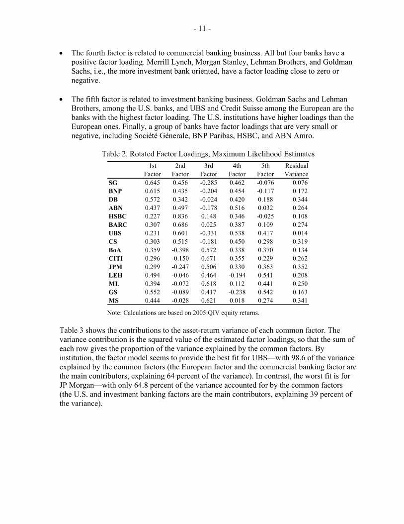
• The fourth factor is related to commercial banking business. All but four banks have a positive factor loading. Merrill Lynch, Morgan Stanley, Lehman Brothers, and Goldman Sachs, i.e., the more investment bank oriented, have a factor loading close to zero or negative.

• The fifth factor is related to investment banking business. Goldman Sachs and Lehman

Brothers, among the U.S. banks, and UBS and Credit Suisse among the European are the banks with the highest factor loading. The U.S. institutions have higher loadings than the European ones. Finally, a group of banks have factor loadings that are very small or negative, including Société Génerale, BNP Paribas, HSBC, and ABN Amro.

Table 2. Rotated Factor Loadings, Maximum Likelihood Estimates

1st Factor

2nd Factor

3rd Factor

4th Factor

5th Factor

Residual Variance

SG 0.645 0.456 -0.285 0.462 -0.076 0.076BNP 0.615 0.435 -0.204 0.454 -0.117 0.172DB 0.572 0.342 -0.024 0.420 0.188 0.344ABN 0.437 0.497 -0.178 0.516 0.032 0.264HSBC 0.227 0.836 0.148 0.346 -0.025 0.108BARC 0.307 0.686 0.025 0.387 0.109 0.274UBS 0.231 0.601 -0.331 0.538 0.417 0.014CS 0.303 0.515 -0.181 0.450 0.298 0.319BoA 0.359 -0.398 0.572 0.338 0.370 0.134CITI 0.296 -0.150 0.671 0.355 0.229 0.262JPM 0.299 -0.247 0.506 0.330 0.363 0.352LEH 0.494 -0.046 0.464 -0.194 0.541 0.208ML 0.394 -0.072 0.618 0.112 0.441 0.250GS 0.552 -0.089 0.417 -0.238 0.542 0.163MS 0.444 -0.028 0.621 0.018 0.274 0.341

Note: Calculations are based on 2005:QIV equity returns. Table 3 shows the contributions to the asset-return variance of each common factor. The variance contribution is the squared value of the estimated factor loadings, so that the sum of each row gives the proportion of the variance explained by the common factors. By institution, the factor model seems to provide the best fit for UBS—with 98.6 of the variance explained by the common factors (the European factor and the commercial banking factor are the main contributors, explaining 64 percent of the variance). In contrast, the worst fit is for JP Morgan—with only 64.8 percent of the variance accounted for by the common factors (the U.S. and investment banking factors are the main contributors, explaining 39 percent of the variance).

- 12 -

Table 3. Variance Contribution

1st Factor

2nd Factor

3rd Factor

4th Factor

5th Factor

Idiosyncratic Variance

SG 0.416 0.208 0.082 0.214 0.006 0.076BNP 0.378 0.189 0.042 0.206 0.014 0.172DB 0.327 0.117 0.001 0.176 0.035 0.344ABN 0.191 0.247 0.032 0.266 0.001 0.264HSBC 0.052 0.698 0.022 0.119 0.001 0.108BARC 0.094 0.470 0.001 0.149 0.012 0.274UBS 0.054 0.361 0.110 0.289 0.174 0.014CS 0.092 0.265 0.033 0.202 0.089 0.319BoA 0.129 0.158 0.328 0.114 0.137 0.134CITI 0.088 0.022 0.450 0.126 0.053 0.262JPM 0.090 0.061 0.256 0.109 0.132 0.352LEH 0.244 0.002 0.215 0.038 0.293 0.208ML 0.155 0.005 0.382 0.013 0.194 0.250GS 0.305 0.008 0.174 0.057 0.294 0.163MS 0.197 0.001 0.386 0.000 0.075 0.341Average 0.187 0.187 0.167 0.139 0.101 0.219

Note: Calculations are based on 2005:QIV equity returns.

VI. COMPUTATION OF THE PROBABILITIES OF DEFAULT

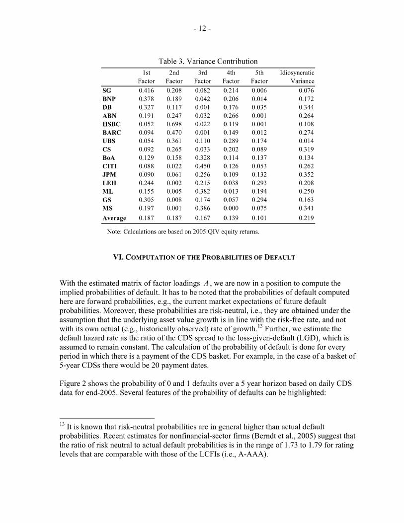
With the estimated matrix of factor loadings A , we are now in a position to compute the implied probabilities of default. It has to be noted that the probabilities of default computed here are forward probabilities, e.g., the current market expectations of future default probabilities. Moreover, these probabilities are risk-neutral, i.e., they are obtained under the assumption that the underlying asset value growth is in line with the risk-free rate, and not with its own actual (e.g., historically observed) rate of growth.13 Further, we estimate the default hazard rate as the ratio of the CDS spread to the loss-given-default (LGD), which is assumed to remain constant. The calculation of the probability of default is done for every period in which there is a payment of the CDS basket. For example, in the case of a basket of 5-year CDSs there would be 20 payment dates. Figure 2 shows the probability of 0 and 1 defaults over a 5 year horizon based on daily CDS data for end-2005. Several features of the probability of defaults can be highlighted:

13 It is known that risk-neutral probabilities are in general higher than actual default probabilities. Recent estimates for nonfinancial-sector firms (Berndt et al., 2005) suggest that the ratio of risk neutral to actual default probabilities is in the range of 1.73 to 1.79 for rating levels that are comparable with those of the LCFIs (i.e., A-AAA).

- 13 -

• The one quarter forward probability of no defaults is very high (0.99 percent). This is typical of CDS baskets of highly rated financial institutions, such as the LCFIs.

• The probability of no default falls systematically from one quarter ahead to 20 quarters

ahead (83.7 percent), logically implying that the market sees the likelihood of defaults increasing as time passes.

• The other side of the coin is that the probability of one default over the next quarter is

very small (0.8 percent) and it increases over the 5 year horizon up to 8.2 percent. Although not shown in the figure, a similar pattern can be observed for the probability of 2 defaults, 3 defaults, etc.

Figure 2. Probability of Default: One- to Twenty-Quarter Ahead

0.80

0.84

0.88

0.92

0.96

1.00

1 2 3 4 5 6 7 8 9 10 11 12 13 14 15 16 17 18 19 200.00

0.02

0.04

0.06

0.08

0.10Probability of no default (left axis)

Probability of one default (right axis)

Note: Calculations are based on end-2005 CDS spreads, correlations, and factor structure.

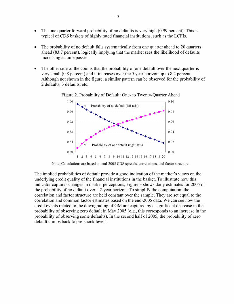
The implied probabilities of default provide a good indication of the market’s views on the underlying credit quality of the financial institutions in the basket. To illustrate how this indicator captures changes in market perceptions, Figure 3 shows daily estimates for 2005 of the probability of no default over a 2-year horizon. To simplify the computation, the correlation and factor structure are held constant over the sample. They are set equal to the correlation and common factor estimates based on the end-2005 data. We can see how the credit events related to the downgrading of GM are captured by a significant decrease in the probability of observing zero default in May 2005 (e.g., this corresponds to an increase in the probability of observing some defaults). In the second half of 2005, the probability of zero default climbs back to pre-shock levels.

- 14 -

Figure 3. Two-Year-Ahead Probability of No Defaults

0.88

0.89

0.90

0.91

0.92

0.93

Jan-05

Feb-05

Mar-05

Apr-05

May-05

Jun-05

Jul-05

Aug-05

Sep-05

Oct-05

Nov-05

Dec-05

GM downgrading

Note: Calculations are based on CDS spreads for 2005 (constant correlation and factor structure).

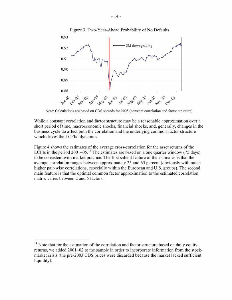
While a constant correlation and factor structure may be a reasonable approximation over a short period of time, macroeconomic shocks, financial shocks, and, generally, changes in the business cycle do affect both the correlation and the underlying common-factor structure which drives the LCFIs’ dynamics. Figure 4 shows the estimates of the average cross-correlation for the asset returns of the LCFIs in the period 2001–05.14 The estimates are based on a one quarter window (75 days) to be consistent with market practice. The first salient feature of the estimates is that the average correlation ranges between approximately 25 and 65 percent (obviously with much higher pair-wise correlations, especially within the European and U.S. groups). The second main feature is that the optimal common factor approximation to the estimated correlation matrix varies between 2 and 5 factors.

14 Note that for the estimation of the correlation and factor structure based on daily equity returns, we added 2001–02 to the sample in order to incorporate information from the stock-market crisis (the pre-2003 CDS prices were discarded because the market lacked sufficient liquidity).

- 15 -

Figure 4. Estimated Correlation and Factor Structure (2001–05)

0.25

0.30

0.35

0.40

0.45

0.50

0.55

0.60

0.65

Apr-0

1Se

p-01

Jan-

02Ju

n-02

Oct-0

2M

ar-0

3Au

g-03

Dec-

03M

ay-0

4Se

p-04

Feb-

05Ju

l-05

Nov-

05

0

1

2

3

4

5

Num

ber of comm

on factors

Avera ge correlation

Note: Estimates are based on daily equity-return data for the 15 LCFIs for 2001–05.

In sum, the rich dynamics in the correlation and common factor structure of the equity returns suggest that a multifactor approach is better suited than a single factor model to compute the probability of default and the pricing of the CDS basket. How sensitive is the implied probability of default to a time-varying correlation and a multifactor representation? Can the multifactor approximation to the correlation matrix serve as a platform to conduct stress test analysis of the LCFIs to macroeconomic and financial shocks? These and other issues involving the sensitivity analysis are examined in the next section.

VII. SENSITIVITY ANALYSIS

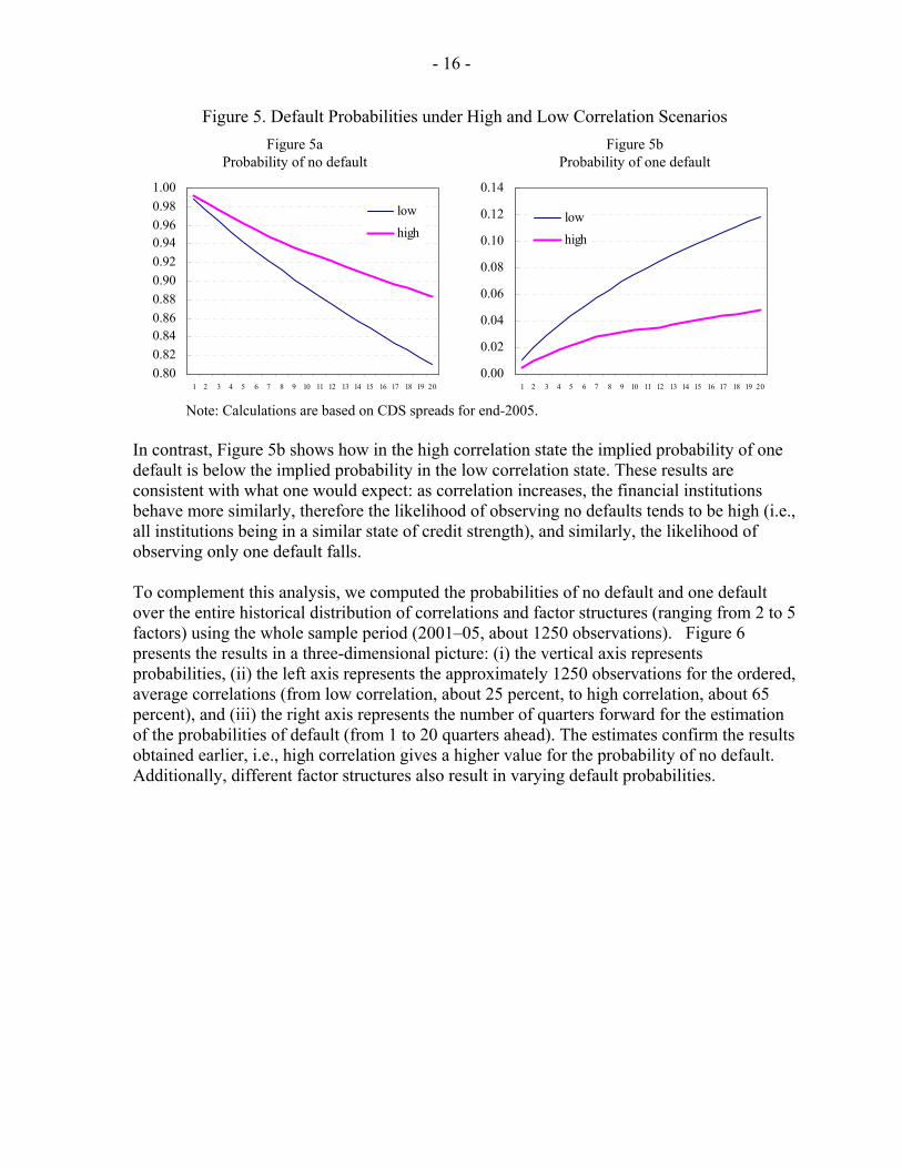
To assess the impact on the implied probability of default of different correlations and their multifactor representation, we selected some extreme correlation values from their observed historical distribution. In particular, we selected the highest and lowest average correlations among those with a 5-factor representation, which correspond to the 99.2 percentile and the 1.3 percentile of the historical distribution of average correlation, respectively. They correspond to the 3-month period ending in January 14, 2004 and October 21, 2002, respectively. Figure 5a shows how in the high-correlation scenario the implied probability of no defaults—over one-quarter to a five-year horizon—is much higher than that in the low-correlation scenario. The computation of the probability of default is again based on end-2005 data on CDS spreads.

- 16 -

Figure 5. Default Probabilities under High and Low Correlation Scenarios

Figure 5a Figure 5b Probability of no default Probability of one default

0.800.820.840.860.880.900.920.940.960.981.00

1 2 3 4 5 6 7 8 9 10 11 12 13 14 15 16 17 18 19 20

low

high

0.00

0.02

0.04

0.06

0.08

0.10

0.12

0.14

1 2 3 4 5 6 7 8 9 10 11 12 13 14 15 16 17 18 19 20

low

high

Note: Calculations are based on CDS spreads for end-2005.

In contrast, Figure 5b shows how in the high correlation state the implied probability of one default is below the implied probability in the low correlation state. These results are consistent with what one would expect: as correlation increases, the financial institutions behave more similarly, therefore the likelihood of observing no defaults tends to be high (i.e., all institutions being in a similar state of credit strength), and similarly, the likelihood of observing only one default falls. To complement this analysis, we computed the probabilities of no default and one default over the entire historical distribution of correlations and factor structures (ranging from 2 to 5 factors) using the whole sample period (2001–05, about 1250 observations). Figure 6 presents the results in a three-dimensional picture: (i) the vertical axis represents probabilities, (ii) the left axis represents the approximately 1250 observations for the ordered, average correlations (from low correlation, about 25 percent, to high correlation, about 65 percent), and (iii) the right axis represents the number of quarters forward for the estimation of the probabilities of default (from 1 to 20 quarters ahead). The estimates confirm the results obtained earlier, i.e., high correlation gives a higher value for the probability of no default. Additionally, different factor structures also result in varying default probabilities.

- 17 -

Figure 6. Probability of default over range of correlation and factor structures

Probability of no default Probability of one default

Note: Calculations are based on CDS spreads for end 2005. Finally, we re-estimated all the probabilities of default for the entire sample of CDS spreads (2003–05). Figure 7 shows the 2-year-ahead probability of zero and one defaults. First, we kept the correlation and factor structure constant and equal to the median average correlation estimated over the period 2001–05 (represented by the thin line in the graph). Second, we let the correlation and factor structure be reestimated over time as new information becomes available using a 3-month estimation window. This results in significant changes in the estimates of probabilities of default (thick line), indicating that updating the correlation structure, as well as its multifactor representation, is critical in the computation of the probabilities of default.

Figure 7. Two-year Ahead Probability of Default: Variable vs. Fixed Correlation and Factors

Probability of no default Probability of one default

0.800.820.840.860.880.900.920.940.96

Jan-03

Jul-03

Jan-04

Jul-04

Jan-05

Jul-05

fixedvariable

0.020.030.040.050.060.070.080.090.10

Jan-03

Jul-03

Jan-04

Jul-04

Jan-05

Jul-05

fixedvariable

Note: “Variable” shows the two-year-ahead probability of default using the rolling estimation of the correlation and factor structure using a 75 day window. “Fixed” corresponds to estimates of the probability of default with a constant correlation structure set equal to the median correlation from its historical distribution (based on 2001–05).

- 18 -

VIII. STRESS TESTING

In the previous section we have shown how the probabilities of default are sensitive to changes in the correlation and in the factor structure. The multifactor structure allows us to analyze also the response of the probabilities of default to shocks in the factors themselves. As we have seen, the estimated factors are in fact related to the state of the financial and macroeconomic conditions in which the LCFIs operate. For example, if a global recession hits both the European and U.S. financial institutions, the probabilities of default are likely to increase. It then becomes important to understand the relative significance of the different channels (i.e., factors) through which this scenario affects the default probabilities of the institutions. Specifically, to implement a stress test, we can estimate the probabilities of default (0 defaults, 1 default, 2 defaults, etc.) conditional on a certain value of the common factor. For example, to examine the effect of a “recession” (“boom”) on a given factor, we can integrate over the set the values of the factor in the left (right) tail of the factor’s distribution (Gibson, 2004). Figure 8 shows such a calculation. We first computed the implied probability of default over the next 5 years (i.e., 20 quarters). Figure 8a shows the probability of zero default (left axis) and one, two, and three defaults (right axis) in the baseline scenario. The baseline-scenario probabilities are computed based on the end-2005 correlation and factor structure (i.e., the 5 factor structure described earlier). In general, given the high quality of the LCFIs the probability of two and three defaults are well below 5 percent even at the 5-year horizon. In contrast to the baseline, when all factors enter simultaneously into a generalized recession, the probabilities of default change substantially. As Figure 8b shows, the probability of zero defaults falls from around 90 percent (one quarter ahead), to around 30 percent (two years ahead), and below ten percent (5 years ahead ). The flip side of the coin is that the probability of one default over a two-year horizon jumps significantly up to about 40 percent. The pattern of the different default probability dynamics in a recession is in fact intuitively very appealing. At longer time horizons, there is a progressive worsening of the credit conditions. This shows up as an increase in the probability of observing a larger number of defaults. 15

15 Indeed, the estimates show that the probability of observing only one default falls after two years and, after three years, the probability of two defaults is even higher than the probability of one default. Between 3 to 5 years ahead, a similar pattern emerges, namely, the probability of observing three defaults increases, rising above the probability of observing two and one defaults, which then start to decline.

- 19 -

Figure 8. Stress Testing: Probabilities of Default Under an “All Factor” Recession Scenario

Figure 8a

0.00

0.20

0.40

0.60

0.80

1.00

1 2 3 4 5 6 7 8 9 10 11 12 13 14 15 16 17 18 19 2 00.000.050.100.150.200.250.300.350.400.45

PD0 PD1 PD2 PD3

Left scale

Right scale

Baseline

Figure 8b

0.00

0.20

0.40

0.60

0.80

1.00

1 2 3 4 5 6 7 8 9 10 11 12 13 14 15 16 17 18 19 2 00.000.050.100.150.200.250.300.350.400.45

All factors in recession

Note: Calculations are based on CDS spreads for end 2005.

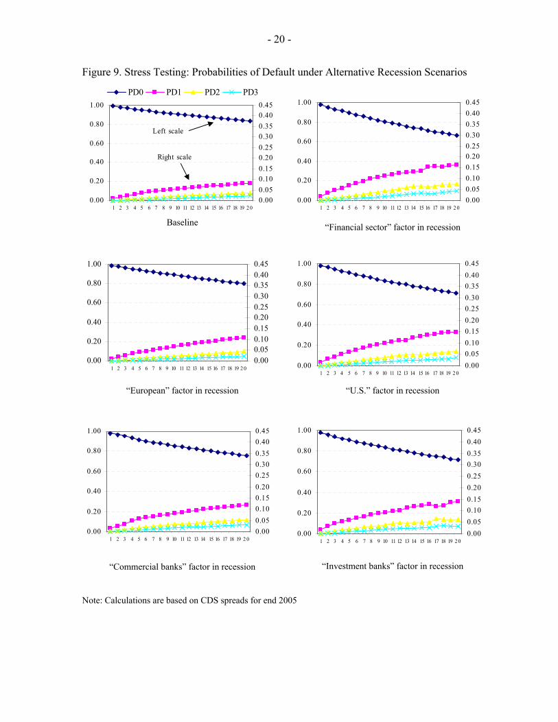
The multifactor framework also allows for an analysis of shocks to each of the factors individually. Figure 9 shows the probability of default under a negative shock (a recession) to each of the 5 factors individually. Under a negative shock to the first factor or, in other words, when the financial-sector factor enters into a recession, the probability of observing zero defaults falls relative to the baseline scenario. This is a result of all the loadings for the first factor being large and positive. Consistently, the probability of observing 1, 2, and 3 defaults rises above the baseline-scenario probabilities. When shocks affect the other 4 factors, similar patterns emerge. However, the overall impact in terms of the probability of default has a comparatively smaller effect than for the first-factor shock, since some of the loadings are small and/or negative. We also conducted a stress test analysis for a positive shock (“boom”) to all factors as well as one factor at a time.16 When all factors are jointly in a boom scenario, most of the probability mass concentrates on zero defaults. In the case of a boom for each factor at a time, the probability of zero defaults also has higher values than in the baseline; however, the probability of observing just one default increases over time relative to the baseline. And, consistently, the probability of observing more than one default falls relative to the baseline.

16 The results of the boom scenarios are available from the authors upon request.

- 20 -

Figure 9. Stress Testing: Probabilities of Default under Alternative Recession Scenarios

0.00

0.20

0.40

0.60

0.80

1.00

1 2 3 4 5 6 7 8 9 10 11 12 13 14 15 16 17 18 19 2 00.000.050.100.150.200.250.300.350.400.45

PD0 PD1 PD2 PD3

Left scale

Right scale

Baseline

0.00

0.20

0.40

0.60

0.80

1.00

1 2 3 4 5 6 7 8 9 10 11 12 13 14 15 16 17 18 19 2 00.000.050.100.150.200.250.300.350.400.45

“Financial sector” factor in recession

0.00

0.20

0.40

0.60

0.80

1.00

1 2 3 4 5 6 7 8 9 10 11 12 13 14 15 16 17 18 19 2 00.000.050.100.150.200.250.300.350.400.45

“European” factor in recession

0.00

0.20

0.40

0.60

0.80

1.00

1 2 3 4 5 6 7 8 9 10 11 12 13 14 15 16 17 18 19 2 00.000.050.100.150.200.250.300.350.400.45

“U.S.” factor in recession

0.00

0.20

0.40

0.60

0.80

1.00

1 2 3 4 5 6 7 8 9 10 11 12 13 14 15 16 17 18 19 2 00.000.050.100.150.200.250.300.350.400.45

“Commercial banks” factor in recession

0.00

0.20

0.40

0.60

0.80

1.00

1 2 3 4 5 6 7 8 9 10 11 12 13 14 15 16 17 18 19 2 00.000.050.100.150.200.250.300.350.400.45

“Investment banks” factor in recession

Note: Calculations are based on CDS spreads for end 2005

- 21 -

IX. CONCLUDING REMARKS

This paper develops a market-based indicator for financial sector surveillance. Building on Hull and White (2005) and Gibson (2004), our approach generalizes Avesani (2005) by adopting a multifactor latent structure in the determination of the default probabilities of a credit default swap basket of large complex financial institutions. Factor analysis shows that the correlation among the financial institutions requires a multifactor representation, which is critical for the computation of the default correlations and, therefore, for the accuracy of this indicator. The identification and estimation of the factors, which drive the covariance-matrix dynamics, offer an opportunity to bring macroeconomic-related factors to bear in a purely financial model. By doing so, we are proposing a new angle from which to approach stress testing. In fact, the impact of changing macroeconomic conditions (e.g., a recession) is directly modeled through shocks to the multifactor structure that is generated within the financial model. Our empirical results based on end-2005 credit default swap spreads and stress testing analysis provide the following insights. First, the two-year forward probability of no default (92 percent) has increased markedly compared to the one observed during the May 2005 credit events related to the downgrading of General Motors (88 percent). Second, the stress-testing results for a scenario where all common factors enter a recession simultaneously show that the two-year forward probability of no default would fall to around 30 percent. And, third, a recession in the U.S. factor, that is, a more similar shock to the May 2005 credit events, which affected mostly U.S. institutions, would result in two-year forward probability of default of about 80 percent. Overall, the results obtained from the application of these shocks unveil a rich set of default probability dynamics and help in identifying the most relevant sources of risk.

- 22 -

References Andersen, Leif, Jakob Sidenius and Susanta Basu, 2003, “All Your Hedges in One Basket,”

Risk, November, pp. 67–72. Anderson, T.W., 2003, An Introduction to Multivariate Analysis, 3rd Edition John Wiley &

Sons (New York). Avesani, Renzo G., 2005, “FIRST: A Market-Based Approach to Evaluate Financial System

Risk and Stability,” Working Paper No. 05/232 (Washington: International Monetary Fund).

Bartlett, M.S., 1950, “Tests of Significance in Factor Analysis,” British Journal of

Psychology, Vol. 3, pp. 77—85. Bank of England, 2004, Financial Stability Review, (London: Bank of England), December. Berndt, A., R. Douglas, D. Duffie, M. Ferguson, and D. Schranz, 2005, “Measuring Default

Risk Premia from Default Swap Rates and EDFs,” (unpublished; Palo Alto: Stanford University).

Black, F., and M. Scholes, 1973, “The Pricing of Options and Corporate Liabilities,” Journal

of Political Economy, Vol. 81, No. 3 (May/June), pp. 637—54. Crockett, Andrew, 2000, “Marrying the Micro- and Macro-Prudential Dimensions of

Financial Stability,” Eleventh International Conference of Banking Supervisors, Basel, September 2000.

Elsinger, Helmut, Alfred Lehar, Martin Summer, and Simon Wells, 2004, “Using Market

Information for Banking System Risk Assessment,”, (unpublished; London: Bank of England).

FitchRatings, 2005, “A Comparative Empirical Study of Asset Correlations,” Structured

Finance, July. Flannery, M.J., and S.M. Sorescu, 1996, “Evidence of Bank Market Discipline in

Subordinated Debenture Yields: 1983–1991,” Journal of Finance 51, (September), pp. 1347–77.

Gibson, Michael, 2004, “Understanding the Risk of Synthetic CDOs” (unpublished

Washington: Federal Reserve Board). Gropp, R., J. Vesala, and G. Vulpes, 2002, “Equity and Bond Market Signals As Leading

Indicators of Bank Fragility,” Working Paper No. 150 (Frankfurt: European Central Bank).

- 23 -

Hawkesby, Christian, Ian Marsh, and Ibrahim Stevens, 2005, “Comovements in the Price of Securities Issued by Large Complex Financial Institutions,” Working Paper No. 256, (London: Bank of England).

Hull, John, and Alan White 2005, “Valuation of a CDO and an Nth -to-default CDS Without

Monte Carlo Simulation,” Journal of Derivatives, Vol. 12, No. 2, pp. 8–23. International Monetary Fund, 2003, “Compilation Guide on Financial Soundness Indicators,”

March draft (Washington: International Monetary Fund). Available on the Internet at http://www.imf.org/external/np/sta/fsi/eng/guide/index.htm.

Kevin J. Stiroh, 2005, “Bank Risk and Revenue Diversification: An Assessment of Using

Equity Returns” (unpublished; New York: Federal Reserve Bank System). Merton, R.C., 1974, “On the Pricing of Corporate Debt: The Risk Structure of Interest

Rates,” Journal of Finance, Vol. 29, pp. 449–70. Pesaran, M.H., T. Schuermann, B.-J. Treutler, 2005, “Global Business Cycle and Credit

Risk, ” Working Paper No. 11493 (Cambridge, Massachusetts: National Bureau of Economic Research).

Vasicek, O., 1987, “Probability of Loss on Loan Portfolio,” KMV Working Paper (San

Francisco: KMV Corporation).