A New Valuation Approach - EUR

ERASMUS UNIVERSITY ROTTERDAM ERASMUS SCHOOL OF ECONOMICS ECONOMICS & BUSINESS MASTER FINANCIAL ECONOMICS MASTER MARKETING

MASTER THESIS

A New Valuation Approach INTEGRATING BIG DATA ANALYTICS TO FORECAST CUSTOMER BEHAVIOR AND DRIVING SHAREHOLDER VALUE

PIETER LIEVENSE July 14, 2016

Erasmus University Rotterdam Erasmus School of Economics Burgemeester Oudlaan 50, 3062 PA Rotterdam, the Netherlands * [email protected] ) +31 643 546 466

2

3

DISCLAIMER

In providing the data used for this thesis, as well as in processing data

in general, the company mentioned in this thesis complies with all

relevant (privacy) laws and regulations.

4

5

© Pieter Lievense, 2016 “A New Valuation Approach – Integrating Big Data Analytics to Forecast Customer Behavior and Driving Shareholder Value” Erasmus University Rotterdam Erasmus School of Economics

Economics & Business Master Financial Economics Master Marketing Master Thesis (32 ECTS)

6

7

Erasmus School of Economics

Prof. Dr. B. Donkers (supervisor Marketing) Drs. H. Haanappel (supervisor Financial Economics)

8

9

Acknowledgements No master thesis is solely the effort of its author. This one is certainly no exception. I would like to thank my

manager, who remains anonymous, for providing me the opportunity in conducting my study.

The first six months of my internship were characterized by creating trust and obtaining support for my study.

An early pre-study concerning the historical development of customer equity compared to the share price, has boosted

the internal trust and needed support. With the support of data-specialists, the development of a custom-built dataset

was now on the go. This particular type of dataset was a first-time attempt for all involved. It provides an integrated

customer-centric view for all products, brands and segments of the firm. My special thanks go to the firm’s senior data

specialist. This dataset would not have been there without his specialized data-architectural knowledge and his support.

I would also like to thank four of his team members who supported in collecting the data for all brands and market

segments.

It is thanks to my colleagues of the teams that I joined that I found my way into the firm’s data-warehouse. They

offered me valuable insights on data-availability. Therefore, many thanks go to all of them. In addition, I would like to

thank the team and its manager that supported in gathering the relevant financials.

I continue by thanking Drs. Hans Haanappel (supervisor for the master Financial Economics) for his input on

the financial valuation part of this study. I have spent many hours on preparing and modeling the data; I would like to

thank Prof. Dr. Bas Donkers (supervisor for the master Marketing) for his highly valuable input on this part.

Rotterdam July 14, 2016

10

11

Abstract The most important intangible asset of a firm are its customers. Why? Because ultimately, paying customers

provide the expected future cash flows which determine the value of a firm. As such, it follows to take the individual

relationship as a starting point for firm valuation. The process of valuation is well established in finance. The most

common used methodology among practitioners and academics is the discounted cash flow approach. Against all odds,

the discounted cash flow methodology does not take the individual customer as central object of analysis, and instead

applies an aggregated ‘product-centric’ analysis in forecasting cash flows. Traditionally, the role of the marketing

department is to advocate the customer within the firm. As a consequence, the department is well informed on detailed

information on every individual relationship it has with its customers. Driven by the rise of big data, marketers can

now analyze and accurately forecast the development of the individual future relationship with the customer. This

forms the foundation for valuation of every individual customer relationship with the firm. The objective of this study

is to develop a new valuation method by integrating big data analytics to forecast customer behavior and drive

shareholder value, bridging the gap between marketing and finance. It demonstrates this new approach in valuation,

based on a combination of existing methods and techniques in finance and quantitative marketing. For this purpose,

it combines publicly available data and big data on customer behavior. This study is successful in finding a substantial

and positive correlation between customer equity and shareholder value. In addition, the analysis, forecast and

valuation of individual customer behavior, leads to an accurate firm valuation in terms of obtained shareholder value

compared to a well calibrated discounted cash flow valuation. It also delivers new insights on value creation. An

example is that the largest customer behavior value driver, in terms of total SHV contribution is ‘retention,’ ranging

between EUR 6.7–10.4b. Another insight example comes from improving the customer probabilities for the customer

behavior value driver ‘defection.’ An improvement in this value driver of 1% yields an incremental SHV of EUR 360–

596m. Overall, the results show that the integration of big data analytics into a valuation context, valuing individual

customer relationships linked to shareholder value is successful, accurate and insightful.

12

13

14

Contents 1. Introduction ............................................................................................................................................................................... 21

2. Theoretical framework and hypotheses ................................................................................................................................ 262.1 Shareholder value and value drivers ................................................................................................................................ 26

2.1.1 Discounted cash flow valuation ............................................................................................................................... 282.2 Marketing and shareholder value ..................................................................................................................................... 29

2.2.1 Customer-based valuation ......................................................................................................................................... 322.2.2 Customer behavior value drivers and forecasting ................................................................................................. 352.2.3 Customer brand choice behavior and forecasting ................................................................................................. 382.2.4 Customer characteristics, relationship age, share of wallet and forecasting ...................................................... 38

2.3 Conceptual model .............................................................................................................................................................. 39

3. Data ............................................................................................................................................................................................. 423.1 Financial data ...................................................................................................................................................................... 42

3.1.1 Historical performance .............................................................................................................................................. 423.2 Integrated customer-centric dataset ................................................................................................................................ 43

3.2.1 Data availability ........................................................................................................................................................... 453.2.2 Descriptive statistics ................................................................................................................................................... 47

4. Methodology .............................................................................................................................................................................. 504.1 Discounted cash flow valuation model .......................................................................................................................... 504.2 Customer-based valuation models .................................................................................................................................. 55

4.2.1 Customer equity valuation model ............................................................................................................................ 554.2.2 Customer behavior based status quo valuation model ......................................................................................... 574.2.3 Customer behavior based valuation model ............................................................................................................ 58

4.2.3.1 Profit regression model ...................................................................................................................................... 624.2.3.2 Behavior logit model .......................................................................................................................................... 63

5. Results......................................................................................................................................................................................... 655.1 Discounted cash flow value .............................................................................................................................................. 655.2 Customer-based values ...................................................................................................................................................... 67

5.2.1 Customer equity value ............................................................................................................................................... 675.2.2 Customer behavior based status quo value ............................................................................................................ 685.2.3 Customer behavior based value ............................................................................................................................... 70

5.2.3.1 Estimation results profit regression models ................................................................................................... 745.2.3.2 Estimation results behavior logit models ........................................................................................................ 77

6. Conclusions ............................................................................................................................................................................... 846.1 Hypotheses testing ............................................................................................................................................................. 856.2 Comparing DCF and CBB valuation models ................................................................................................................ 87

6.2.1 Pros and cons .............................................................................................................................................................. 89

15

6.3 Limitations of the study .................................................................................................................................................... 896.4 Managerial implications ..................................................................................................................................................... 91

6.4.1 Directions for future studies ..................................................................................................................................... 926.5 System requirements .......................................................................................................................................................... 93

Appendix ........................................................................................................................................................................................ 94

References .................................................................................................................................................................................... 104

16

Index of figures Figure 1 Shareholder value drivers (Koller et al. 2010) ........................................................................................................... 26

Figure 2 Customer behavior spectrum ...................................................................................................................................... 35

Figure 3 Conceptual model ......................................................................................................................................................... 41

Figure 4 Share price index 2003–2014 ....................................................................................................................................... 42

Figure 5 DCF framework ............................................................................................................................................................ 51

Figure 6 Revenues (EURm) ........................................................................................................................................................ 52

Figure 7 Revenue growth (YoY%) ............................................................................................................................................. 52

Figure 8 EBITDA (EURm) ........................................................................................................................................................ 52

Figure 9 EBITDA-margin (%) .................................................................................................................................................... 52

Figure 10 CAPEX to depreciation ratio (x) .............................................................................................................................. 52

Figure 11 Net working capital (EURm) .................................................................................................................................... 52

Figure 12 Tax rate (%) .................................................................................................................................................................. 52

Figure 13 FCF (EURm) ............................................................................................................................................................... 52

Figure 14 Cash flow from operations 2003–2014 (EURm) (m) ........................................................................................... 56

Figure 15 Average annual retention rate 2003–2014 (r) ......................................................................................................... 56

Figure 16 Average post tax WACC 2003–2014 (d) ................................................................................................................. 56

Figure 17 Growth rate after customer defection 2003–2014 (g) ........................................................................................... 56

Figure 18 CBB valuation framework ......................................................................................................................................... 59

Figure 19 DV distribution log transformed EBITDA - CM ................................................................................................. 60

Figure 20 DV distribution log transformed EBITDA - BM (excl. outliers) ........................................................................ 60

Figure 21 Predictor distribution log transformed EBITDA - CM ........................................................................................ 61

Figure 22 Predictor distribution log transformed EBITDA - BM (excl. outliers) .............................................................. 61

Figure 23 Shareholder value ranges per valuation model (EURm) ....................................................................................... 65

Figure 24 Customer equity and share price 2003–2014 .......................................................................................................... 67

Figure 25 Shareholder value contribution range per customer behavior value driver (95% CI – EURm) .................... 73

Figure 26 Shareholder value impact by 1% improvement per customer behavior value driver (95% CI – EURm) .... 73

Figure 27 Customer equity scenario forecast by DCF and CBB valuation 2015–2018 ..................................................... 84

17

Index of tables Table 1 Competitive advantage drivers (Koller et al. 2010) ................................................................................................... 27 Table 2 Growth drivers (Koller et al. 2010) .............................................................................................................................. 27 Table 3 Marketing assets and actions contribution to shareholder value (Srinivasan & Hanssens 2009) ...................... 31 Table 4 Quick overview integrated customer-centric dataset ................................................................................................ 43 Table 5 EBITDA-margins 2014 ................................................................................................................................................. 43 Table 6 Pearson correlations of third party customer characteristics and EBITDA 2013–2014 (r-coefficient) ........... 45 Table 7 Data availability by BSP-combination per period ...................................................................................................... 47 Table 8 Descriptive statistics ....................................................................................................................................................... 48 Table 9 Pearson correlation matrix customer-behavior in 2013 and 2014 CM .................................................................. 48 Table 10 Pearson correlation matrix customer-behavior in 2013 and 2014 BM ................................................................ 49 Table 11 Free cash flow definition ............................................................................................................................................. 51 Table 12 DCF valuation ............................................................................................................................................................... 65 Table 13 Discounted cash flow statement ................................................................................................................................ 66 Table 14 Weighted average cost of capital ................................................................................................................................ 66 Table 15 Customer equity (EURb) ............................................................................................................................................. 68 Table 16 Customer behavior based status quo valuation ....................................................................................................... 68 Table 17 Customer equity valuation (EURm) .......................................................................................................................... 69 Table 18 Customer behavior based status quo cash flow statement .................................................................................... 70 Table 19 CBB forecasted EBITDA composition .................................................................................................................... 70 Table 20 Customer behavior based valuation (EURm) .......................................................................................................... 71 Table 21 Customer behavior based cash flow statement (EURm) ....................................................................................... 72 Table 22 Estimation results profit regression model (CM) .................................................................................................... 75 Table 23 Estimation results profit regression model (BM) .................................................................................................... 76 Table 24 Estimation results behavior logit models CM .......................................................................................................... 79 Table 25 Estimation results behavior logit models BM .......................................................................................................... 81 Table 26 Summary of hypotheses-testing results ..................................................................................................................... 85 Table 27 Comparing DCF and CBB valuation model ............................................................................................................ 88 Table 28 Pros and cons of DCF and CBB valuation models ................................................................................................ 89 Table 29 Historical financials ...................................................................................................................................................... 94 Table 30 Historical KPIs ............................................................................................................................................................. 95 Table 31 One-to-one relations [1 out of 2] ............................................................................................................................... 96 Table 32 Descriptive statistics: purchase rates ......................................................................................................................... 98 Table 33 Ownership correlations 2013-2014 (Pearson correlation r-coefficient) ............................................................... 99 Table 34 Forecast on key value drivers ................................................................................................................................... 100 Table 35 Forecasted financials .................................................................................................................................................. 101 Table 36 DCF valuation scenario analysis .............................................................................................................................. 102 Table 37 Input customer equity forecast 2015–2018 ............................................................................................................ 103

18

Index of equations Eq. 1 ........................................... 28

Eq. 2 ........................................... 28

Eq. 3 ........................................... 29

Eq. 4 ........................................... 29

Eq. 5 ........................................... 29

Eq. 6 ........................................... 29

Eq. 7 ........................................... 30

Eq. 8 ........................................... 33

Eq. 9 ........................................... 34

Eq. 10 ......................................... 34

Eq. 11 ......................................... 44

Eq. 12 ......................................... 44

Eq. 13 ......................................... 44

Eq. 14 ......................................... 45

Eq. 15 ......................................... 50

Eq. 16 ......................................... 50

Eq. 17 ......................................... 53

Eq. 18 ......................................... 53

Eq. 19 ......................................... 53

Eq. 20 ......................................... 53

Eq. 21 ......................................... 53

Eq. 22 ......................................... 53

Eq. 23 ......................................... 53

Eq. 24 ......................................... 54

Eq. 25 ......................................... 54

Eq. 26 ......................................... 54

Eq. 27 ......................................... 54

Eq. 28 ......................................... 55

Eq. 29 ......................................... 55

Eq. 30 ......................................... 57

Eq. 31 ......................................... 57

Eq. 32 ......................................... 57

Eq. 33 ......................................... 57

Eq. 34 ......................................... 58

Eq. 35 ......................................... 58

Eq. 36 ......................................... 58

Eq. 37 ......................................... 58

Eq. 38 ......................................... 59

Eq. 39 ......................................... 60

Eq. 40 ......................................... 60

Eq. 41 ......................................... 61

Eq. 42 ......................................... 61

Eq. 43 ......................................... 61

Eq. 44 ......................................... 62

Eq. 45 ......................................... 62

Eq. 46 ......................................... 63

Eq. 47 ......................................... 63

Eq. 48 ......................................... 63

Eq. 49 ......................................... 64

Eq. 50 ......................................... 64

Eq. 51 ......................................... 64

Eq. 52 ......................................... 64

19

List of abbreviations

BS Balance sheet BSP Brand segment product CAPEX Capital expenditures CBB Customer behavior based CBV Customer-based valuation CE Customer equity CF Cash flow CFO Cash flow from operations CLV Customer lifetime value CV Continuing value DCF Discounted cash flow DV Dependent variable EBITDA Earnings before interest, taxes, depreciation, and amortization EMH Efficient market hypotheses EV Enterprise value FCF Free cash flow IV Independent variable KPI Key performance indicator MARKET CAP Market capitalization NOA Non-operating assets NOPLAT Net operating profit less adjusted taxes NPV Net present value NWC Net working capital P&L Profit & loss PP Planning period PV Present value ROIC Return on invested capital RONIC Return on new invested capital SHV Shareholder value SOW Share of wallet YOY Year on year

20

21

1. Introduction

“Customers are the pulse; they provide cash flows – the vital sign of life in a firm” 1

Pieter Lievense (2013–2014)

Originally this is a quote from Jack Welch, retired CEO of General Electric Inc. (1981–2001). However, it is

rewritten to what I believe really is the pulse of a firm: its customers! Ultimately, its them paying bills and thus providing

CFs to the firm. This makes customers the most important intangible asset of a firm, and therefore should be carefully

managed and valued (Gupta & Lehmann 2003). Valuing assets is traditionally a specialty within the finance domain

which is underlined by one of its principles: “if it doesn’t create cash flow, it doesn’t create shareholder value” (Koller

et al. 2010). In addition to finance, the marketing domain is emerging as the specialist in valuing individual customers,

as described in the relatively recent emerged CBV literature; introducing concepts like ‘CLV.’ Therefore, this study

aims to develop a new approach in valuation, combining methods from both quantitative marketing and finance,

integrating big data. The main model, an algorithm driven valuation model, analyzes, forecasts and values customer

behavior, directly linking customers to SHV.

Problem background | The main challenge for senior executives is to create sustainable SHV (Koller et al.

2010). This is accomplished by developing successful strategies that drive future CFs (Koller et al. 2010). In order to

determine the impact of future strategies on CFs, senior executives have to continuously translate and understand how

their strategic choices affect SHV (Koller et al. 2010; Srinivasan & Hanssens 2009). This process is called ‘the firm value

adjustment process’ (Koller et al. 2010; Srinivasan & Hanssens 2009). First, based on their strategic options the value per

share is determined for each scenario, commonly using a DCF valuation model (Koller et al. 2010). Next, based on

the estimated outcome(s) senior executives start managing the expectations of the investor community (Koller et al. 2010).

However, based on their personal view and interpretation of strategic choices investors develop their own expectation

on future CFs (Srinivasan & Hanssens 2009). Different earning expectations lead to trading activity, resulting into the

firm’s share price, hence SHV (Koller et al. 2010; Srinivasan & Hanssens 2009). A down trending share price is

perceived as a failure of senior executive strategic decision making (Koller et al. 2010). An upwards trending share

price is perceived as the opposite (Koller et al. 2010). However, this comes with the risk of getting trapped in the so

called ‘expectations treadmill’ (Koller et al. 2010). Managing down market expectations, or ‘damage control’ is a very hard

task (Koller et al. 2010). This ‘thin line’ between ‘success’ and ‘failure’ creates the need for data driven decision making

(Manyika et al. 2011). According to Manyika et al. (2011) sophisticated big data analytics can substantially improve the

senior executive decision making process. This potentially improves senior executives’ strategy development, future

value assessment and expectations management, ultimately increasing SHV creation (Manyika et al. 2011). A very

promising development in big data analytics is that every day big data becomes bigger and analysis gets more

sophisticated (Arthur 2013). More information on customer preference and other types of customer behavior becomes

available together with the increase of computing and applications power. This makes big data analytics increasingly

important (Arthur 2013), which is also recognized by the World Economic Forum (Davos, Switzerland 2012). The

forum declared big data as a new asset class (Lohr 2012), underlined by that year's payoff: “big data, big impact.” That

the impact and applications of big data analytics are no longer ignored is confirmed by the study of the McKinsey

Global Institute – MGI and McKinsey’s Business Technology Office (Manyika et al. 2011). Manyika et al. (2011)

1 The original quote reads: “cash flow is the pulse – the vital sign of life in a firm.”

22

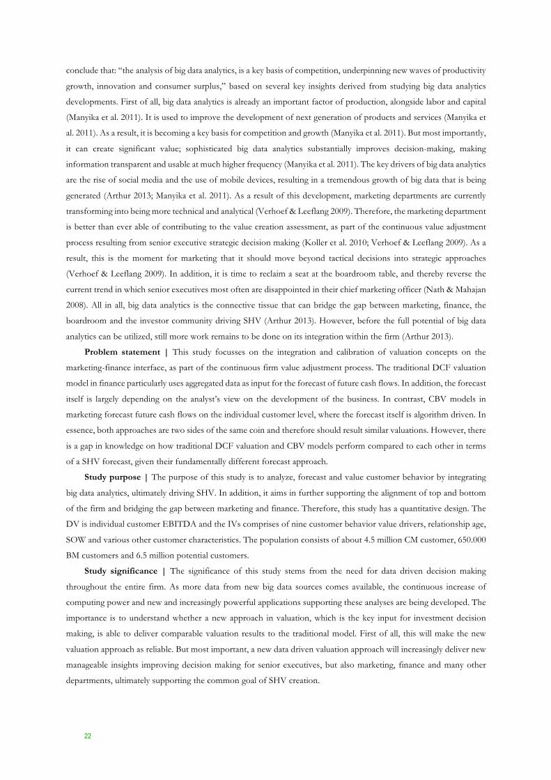
conclude that: “the analysis of big data analytics, is a key basis of competition, underpinning new waves of productivity

growth, innovation and consumer surplus,” based on several key insights derived from studying big data analytics

developments. First of all, big data analytics is already an important factor of production, alongside labor and capital

(Manyika et al. 2011). It is used to improve the development of next generation of products and services (Manyika et

al. 2011). As a result, it is becoming a key basis for competition and growth (Manyika et al. 2011). But most importantly,

it can create significant value; sophisticated big data analytics substantially improves decision-making, making

information transparent and usable at much higher frequency (Manyika et al. 2011). The key drivers of big data analytics

are the rise of social media and the use of mobile devices, resulting in a tremendous growth of big data that is being

generated (Arthur 2013; Manyika et al. 2011). As a result of this development, marketing departments are currently

transforming into being more technical and analytical (Verhoef & Leeflang 2009). Therefore, the marketing department

is better than ever able of contributing to the value creation assessment, as part of the continuous value adjustment

process resulting from senior executive strategic decision making (Koller et al. 2010; Verhoef & Leeflang 2009). As a

result, this is the moment for marketing that it should move beyond tactical decisions into strategic approaches

(Verhoef & Leeflang 2009). In addition, it is time to reclaim a seat at the boardroom table, and thereby reverse the

current trend in which senior executives most often are disappointed in their chief marketing officer (Nath & Mahajan

2008). All in all, big data analytics is the connective tissue that can bridge the gap between marketing, finance, the

boardroom and the investor community driving SHV (Arthur 2013). However, before the full potential of big data

analytics can be utilized, still more work remains to be done on its integration within the firm (Arthur 2013).

Problem statement | This study focusses on the integration and calibration of valuation concepts on the

marketing-finance interface, as part of the continuous firm value adjustment process. The traditional DCF valuation

model in finance particularly uses aggregated data as input for the forecast of future cash flows. In addition, the forecast

itself is largely depending on the analyst’s view on the development of the business. In contrast, CBV models in

marketing forecast future cash flows on the individual customer level, where the forecast itself is algorithm driven. In

essence, both approaches are two sides of the same coin and therefore should result similar valuations. However, there

is a gap in knowledge on how traditional DCF valuation and CBV models perform compared to each other in terms

of a SHV forecast, given their fundamentally different forecast approach.

Study purpose | The purpose of this study is to analyze, forecast and value customer behavior by integrating

big data analytics, ultimately driving SHV. In addition, it aims in further supporting the alignment of top and bottom

of the firm and bridging the gap between marketing and finance. Therefore, this study has a quantitative design. The

DV is individual customer EBITDA and the IVs comprises of nine customer behavior value drivers, relationship age,

SOW and various other customer characteristics. The population consists of about 4.5 million CM customer, 650.000

BM customers and 6.5 million potential customers.

Study significance | The significance of this study stems from the need for data driven decision making

throughout the entire firm. As more data from new big data sources comes available, the continuous increase of

computing power and new and increasingly powerful applications supporting these analyses are being developed. The

importance is to understand whether a new approach in valuation, which is the key input for investment decision

making, is able to deliver comparable valuation results to the traditional model. First of all, this will make the new

valuation approach as reliable. But most important, a new data driven valuation approach will increasingly deliver new

manageable insights improving decision making for senior executives, but also marketing, finance and many other

departments, ultimately supporting the common goal of SHV creation.

23

Academic relevance | As far as my knowledge of the concerning academic literature reaches there has never

been a comparison of a DCF valuation model and a CBV model. Therefore, the academic relevance of this study stems

from its focus on ‘finalytics,’ the point where analytics and finance meet. This study demonstrates a new valuation

approach based on when the best of both academic worlds in quantitative marketing and corporate finance meet. It

combines and integrates value relevant concepts, methods and models from both fields. Or in other words, the advance

in science from this study comes from the merger of a DCF valuation model and a CBV model, complementing each

other. However, the real advance in science stems from the fact that researchers have not shown a direct link between

the forecast of individual customer behavior and its impact on SHV.

Central question | The central question of this study in developing and calibrating a new approach in valuation

that integrates big data analytics, bridging the gap between marketing and finance, is:

DOES INDIVIDUAL CUSTOMER BEHAVIOR DRIVE SHAREHOLDER VALUE?

Sub-questions | Before answering this central question more investigation is required, resulting in various sub-

questions. It is important to understand the concept of value, how value is build up and how the traditional DCF

valuation model in finance determines SHV, thus resulting in the sub-questions:

What is shareholder value?

How is it driven?

How is it derived?

Given that the marketing department is the customer’s ambassador within the firm, and its ultimate goal is to

maximize individual customer profitability, the sub-question is:

Does marketing drive shareholder value?

Given the recently emerged literature stream of CBV in marketing, it is important to understand the concept of

customer-based valuation, what drives customer value and how it can be determined. Therefore, the associated sub-

questions are:

What is customer based value?

How is it driven?

How is it derived?

Given that customer behavior drives customer profitability and customer profitability drives value, the final sub-

questions are:

What is customer behavior?

How does it drive value?

24

Research design | This study uses two main sources of data. On the one hand it uses publicly available firm

financials and on the other hand it heavily relies on large quantities of big data containing customer behavior. The

collection of data from the firm’s various data sources is conducted through database software Microsoft SQL. Five

of the firm’s top data specialists and myself have built an integrated customer centric dataset, combining about 12

million customers (CM: 4.5m; BM: 0.6m and potential: 6.5m), 4 brands, 2 market segments and 29 products. These

main data sources serve as input for two main models. First, a traditional DCF valuation model is used to forecast

future cash flows during a 4-year PP (2015–2018) and derive SHV. The valuation process comprises of four steps: (1)

understanding industry dynamics, (2) understanding competitive position and strategy, (3) analyzing historical

performance and (4) discounting and valuing cash flows. The focus of the first main model in this study is on the last

part of the process. This consist of (4a) identifying key value drivers, (4b) forecasting operating value drivers (P&L, BS

and CF), (4c) determining the WACC, (4d) estimating the CV, and finally (4d) estimating the EV and equity value. In

addition, sensitivity analysis is applied by computing three different scenarios. The second model is an algorithm driven

model, analyzing, forecasting and valuing customer behavior. This so called CBB valuation model is developed based

on various concepts in CBV, rooted in recently emerged marketing literature. The forecast of the model is driven by

18 estimated behavior logit models and 2 profit regression models. The number of predictors for the different models

varies between approximately 60–115. The 18 behavior logit models forecast customer behavior, which serves as input

for the forecast of customer profitability in both profit regression models. The behavior logit and profit regression

models are complemented with additional predictors based on customer characteristics like: relationship age, SOW

and many more. The model forecasts customer behavior and profitability during a 4-year PP (2015–2018) for 3

different scenarios. This results in the calculation of 216 different equations, producing 2 billion estimated probabilities.

Ultimately, for every individual customer an EBITDA forecast is obtained which is finally translated into SHV, hence

equity value. In addition, the second model delivers new and highly valuable insights for senior executives and

managers in their challenge to increase the creation of SHV.

Assumptions | Several assumptions underlie the DCF valuation model. First of all, it assumes that the firm is

all equity financed, so that the financing effects are incorporated in the valuation through the WACC. Then, in

determining the CV it assumes that the firm maintains a competitive advantage in the near future, thus generating a

RONIC higher than the WACC. Finally, in determining the WACC the %& is set to 1.5%; it assumes that current yield

on a ten year German government bond is too low and thus will overestimate the CV of the firm, as it is expected that

yields will rise in the future. Also several assumptions underlie the intermediate CBB status quo valuation model. It

assumes that the EBITDA realized at time ' (2014) simply remains constant during the planning period (2015–2018).

Then, there are also assumptions underlying the algorithm driven CBB valuation model. First, there are several

assumptions with regards to the new developed integrated customer centric dataset. The dataset contains on average

for 88% of unique customers, as it has a location based structure. Therefore, it assumes that each location equals a

unique customer. In determining the DV it assumes that the historical EBITDA-margins remain stable overtime. It

also assumes that for each year of the PP the outlier EBITDA grows by the forward looking inflation rate fixed at

1.5%. In addition, it assumes that the customers driving the outlier EBITDA remain with the firm during the PP, so

that incorporating the retention rate (r) is not needed. Then, concerning the CBB valuation model itself it assumes that

for the forecast all customer characteristic predictors (relationship age, SOW, etc.), observed in 2014, remain stable

over time. The final assumption underlies the forecast of the CE model, it assumes a forward looking retention rate

(%()*,-).), discount rate (/()*,-).) and growth rate (0()*,-).).

25

Scope | The geographical scope of this study concerns the market in which the firm is active in. Only the firm’s

four major brands are included, excluding four relatively small brands. As a result, the generalizability of the study is

very limited.

Summary | This study aims to develop a new approach in valuation, by integrating big data analytics in order to

analyze, forecast and value customer behavior driving SHV. Therefore, it covers four areas. The data that is used as

input for both main models DCF valuation and CBB valuation is discussed, in addition elaborates on the challenges

concerning the development of the integrated customer-centric dataset. It continuous by presenting the used

methodologies in finance and marketing. It also describes how the different models are integrated and merged with

each other. The results present highly valuable new insights arising from this new approach in valuation, driving

improved strategic decision making and the execution of tactics. It ends by concluding and comparing both models,

its pros and cons and the limitations of the study. It also describes directions for future studies. However, it will start

next with discussing origins of SHV and how its driven on the various levels of the firm. This is followed by a brief

review of the most frequently used approach by practitioners and academics in valuation: the DCF valuation model,

rooted in finance literature. Then, it moves on to the marketing section of this study where the contribution of this

domain to SHV is discussed. This includes a review and application of the fundamentals of CLV and CE, forming the

building blocks of CBV. In addition, the value drivers in customer behavior are presented and discussed,

complemented by a review of brand choice behavior and customer characteristics. Finally, the conceptual model is

presented, resulting from the theoretical framework.

26

2. Theoretical framework and hypotheses

“Integrating big data analytics to forecast customer behavior and driving shareholder value”

The theory chapter will broadly cover two literature streams. First, from a finance perspective it describes the

concept of SHV, its drivers and how it can be derived. Then, from a marketing perspective it describes the concept of

CLV and CE, their drivers and how both can be derived. It is remarkable how similar both theoretical concepts are,

however in practice they tend to be far apart. Therefore, the objective of this chapter is to bridge the gap between both

domains. More specific, while describing both subjects it builds the practical link between the concept of CE and SHV

by integrating big data analytics. In doing so, it starts with finance theory describing SHV and its fundamental value

drivers, followed by a brief introduction to DCF valuation theory. A more detailed description on the DCF valuation

method will be covered in the methodology chapter. Then, it switches to marketing theory describing the empirical

findings of marketing’s contribution to SHV. First, it reviews CBV theory, covering the concepts of CLV and CE.

Then, the fundamental value drivers in customer purchase-behavior are discussed. CBV heavily relies on large

quantities of data containing these behaviors. The concept of big data and its relation to valuation and the boardroom’s

relation to value are described previously. Finally, it concludes by presenting the conceptual model derived from theory.

It visualizes the parallelism between the conceptual models of DCF and CBB valuation; two sides of the same coin in

determining and driving SHV.

2.1 Shareholder value and value drivers

“Shareholders value value”

Koller et al. (2010)

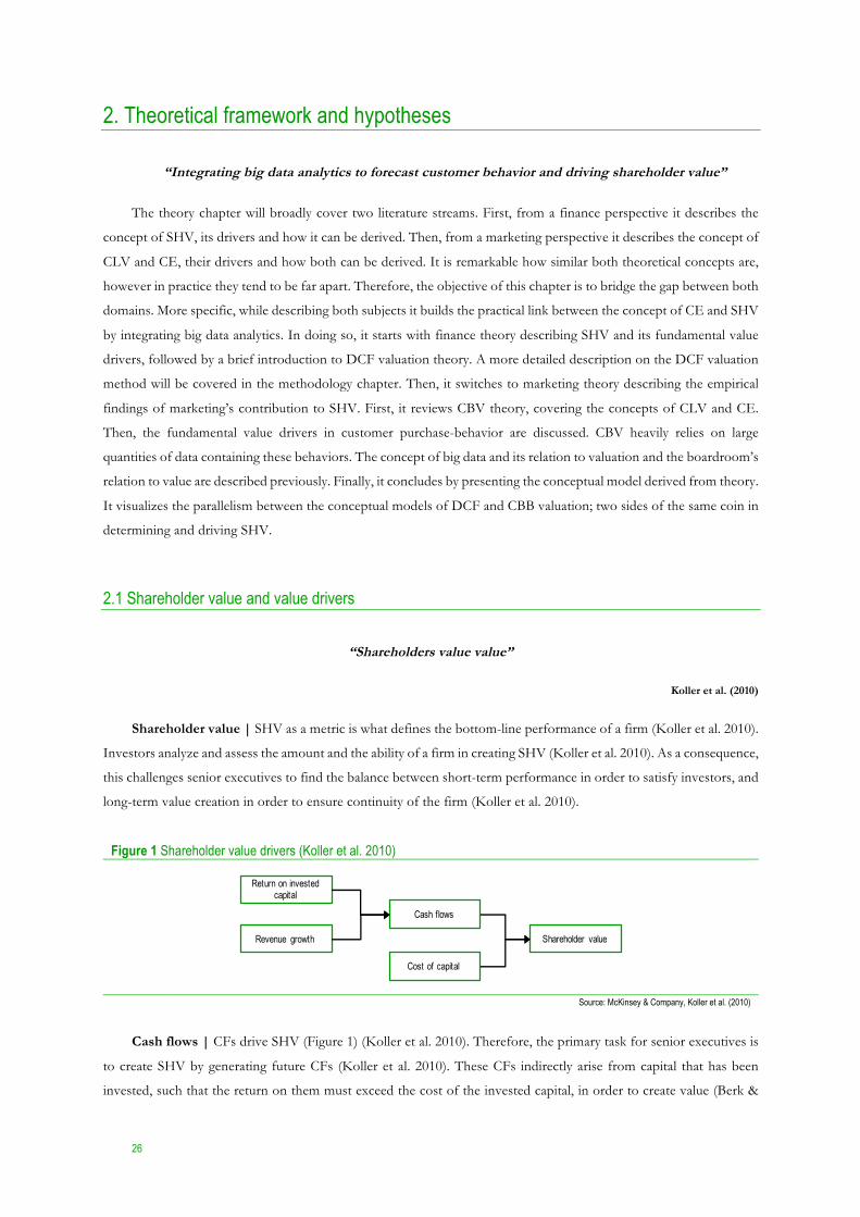
Shareholder value | SHV as a metric is what defines the bottom-line performance of a firm (Koller et al. 2010).

Investors analyze and assess the amount and the ability of a firm in creating SHV (Koller et al. 2010). As a consequence,

this challenges senior executives to find the balance between short-term performance in order to satisfy investors, and

long-term value creation in order to ensure continuity of the firm (Koller et al. 2010).

Figure 1 Shareholder value drivers (Koller et al. 2010)

Source: McKinsey & Company, Koller et al. (2010)

Cash flows | CFs drive SHV (Figure 1) (Koller et al. 2010). Therefore, the primary task for senior executives is

to create SHV by generating future CFs (Koller et al. 2010). These CFs indirectly arise from capital that has been

invested, such that the return on them must exceed the cost of the invested capital, in order to create value (Berk &

Shareholder value

Cash flows

Cost of capital

Return on invested capital

Revenue growth

27

DeMarzo 2007). Modigliani & Miller (1958) showed that senior executives should focus on increasing CFs. They argue

that changes in capital structure that do not change the overall CFs generated by the firm, do not affect SHV. This is

in accordance with a quote of Koller et al. (2010): “if you can’t pinpoint the tangible source of value creation, you’re

probably looking at an illusion.” However, if tax deductibility of debt related interest payments changes the firms CFs,

then this does create value (Koller et al. 2010). Creating value, by generating future CFs is surrounded by uncertainty,

which needs to be taken into account (Koller et al. 2010).

Cost of capital | The COC reflects the price of future CF risk (Koller et al. 2010), resulting from the time value

of money on future CFs (Berk & DeMarzo 2007). The COC, also known as the discount rate, represents at the firm

side the cost of invested capital, as to investors it represents the expected return on invested capital (Berk & DeMarzo

2007). The returns to both equity and debt suppliers are weighted, this results in the WACC (Berk & DeMarzo 2007).

Return on invested capital | Improving ROIC relative to the COC drives SHV (Koller et al. 2010). A good

strategy is the foundation for improvements in ROIC (Marshall 1890; Porter 1980). Senior executives who have

developed a successful strategy deliver the firm a competitive advantage (Koller et al. 2010). The process of continuously

seeking and exploiting new sources of competitive advantage is vital for long-term SHV creation (Koller et al. 2010).

This enables the firm to charge a price premium or to produce with a cost and capital efficiency2 or a combination of both,

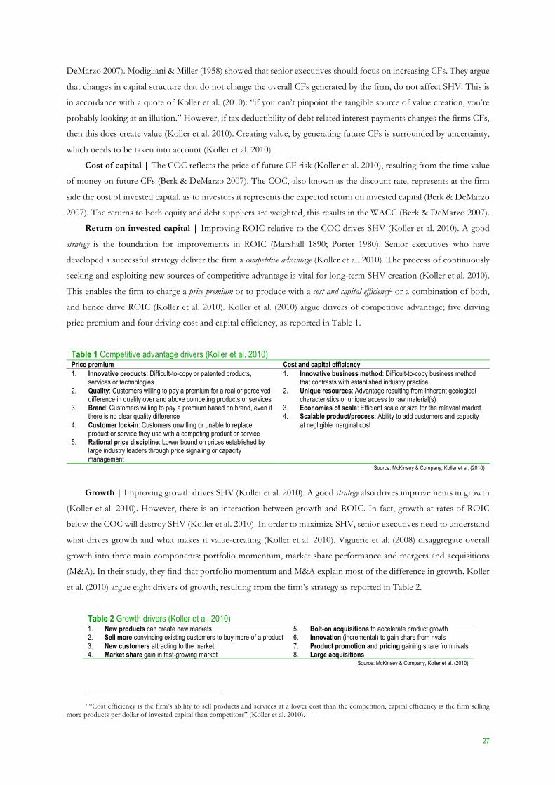
and hence drive ROIC (Koller et al. 2010). Koller et al. (2010) argue drivers of competitive advantage; five driving

price premium and four driving cost and capital efficiency, as reported in Table 1.

Table 1 Competitive advantage drivers (Koller et al. 2010) Price premium Cost and capital efficiency 1. Innovative products: Difficult-to-copy or patented products,

services or technologies 2. Quality: Customers willing to pay a premium for a real or perceived

difference in quality over and above competing products or services 3. Brand: Customers willing to pay a premium based on brand, even if

there is no clear quality difference 4. Customer lock-in: Customers unwilling or unable to replace

product or service they use with a competing product or service 5. Rational price discipline: Lower bound on prices established by

large industry leaders through price signaling or capacity management

1. Innovative business method: Difficult-to-copy business method that contrasts with established industry practice

2. Unique resources: Advantage resulting from inherent geological characteristics or unique access to raw material(s)

3. Economies of scale: Efficient scale or size for the relevant market 4. Scalable product/process: Ability to add customers and capacity

at negligible marginal cost


Growth | Improving growth drives SHV (Koller et al. 2010). A good strategy also drives improvements in growth

(Koller et al. 2010). However, there is an interaction between growth and ROIC. In fact, growth at rates of ROIC

below the COC will destroy SHV (Koller et al. 2010). In order to maximize SHV, senior executives need to understand

what drives growth and what makes it value-creating (Koller et al. 2010). Viguerie et al. (2008) disaggregate overall

growth into three main components: portfolio momentum, market share performance and mergers and acquisitions

(M&A). In their study, they find that portfolio momentum and M&A explain most of the difference in growth. Koller

et al. (2010) argue eight drivers of growth, resulting from the firm’s strategy as reported in Table 2.

Table 2 Growth drivers (Koller et al. 2010) 1. New products can create new markets 2. Sell more convincing existing customers to buy more of a product 3. New customers attracting to the market 4. Market share gain in fast-growing market

5. Bolt-on acquisitions to accelerate product growth 6. Innovation (incremental) to gain share from rivals 7. Product promotion and pricing gaining share from rivals 8. Large acquisitions


2 “Cost efficiency is the firm’s ability to sell products and services at a lower cost than the competition, capital efficiency is the firm selling

more products per dollar of invested capital than competitors” (Koller et al. 2010).

28

New products typically create more SHV, while acquisitions typically create the least (Koller et al. 2010). As Koller

et al. (2010) say: “the crucial point in creating SHV is that revenue growth is not all that matters, it is the value created

per euro of additional revenues that drives the true creation of SHV.” SHV, CFs, COC, ROIC and growth are tightly

linked (Koller et al. 2010). This relation is mathematically expressed in the key value driver formula (Eq. 1) (Koller et

al. 2010):

123( =56789:()* 1 −

=(0()*)

@6AB(C9BB( − =(0()*)

Eq. 1

Where 56789:(DE is the next period’s net operating profit less adjusted taxes, representing the profits generated

from the firm’s core operation after subtracting the income taxes related to these operations (a proxy for CF) and

=(0()*) is the expected growth rate in perpetuity. As Jiang & Koller (2007) say: “the right balance between growth

and ROIC is critically important to SHV creation.”

2.1.1 Discounted cash flow valuation

“If it doesn’t increase cash flow, it doesn’t create value3”

Koller et al. (2010)

As has become clear the creation of SHV is the primary task of a firm (Koller et al. 2010). Senior executives

should focus on increasing CFs by investing capital at a ROIC larger than the COC (Koller et al. 2010; Modigliani &

Miller 1958). In order to determine the amount of SHV generated by the firm, forecasted future CFs need to be

discounted with a discount rate (Berk & DeMarzo 2007; Koller et al. 2010).

Discounted cash flow valuation | DCF valuation is based on the key value driver formula (Eq. 1), representing

the concept governing the theory of valuation (Koller et al. 2010). However, in practice this formula is not used for

firm valuation (Koller et al. 2010). It is too restrictive; it assumes a constant ROIC and growth rate going forward

(Koller et al. 2010). For firms whose key value drivers are expected to change, the DCF valuation model offers more

flexibility in forecasting (Koller et al. 2010). DCF valuation is used for valuing firms, projects or assets using the

concept of the time value of money (Berk & DeMarzo 2007). In his book ‘theory of interest’, Fisher (1930) expressed

as first DCF valuation in modern economic terms. Since then, several valuation methods have emerged, nevertheless

DCF valuation still remains favorite of practitioners and academics (Koller et al. 2010). It relies solely on CFs in and

out of the firm rather than on accounting based earnings, which explains its popularity according to Koller et al. (2010).

Discounted cash flow valuation process | The DCF valuation process for valuing a firm’s common equity is

described by Koller et al. (2010) in a three-part process. First, the value of the firm’s operations (Eq. 2) needs to be derived,

consisting of the PV of the estimated future FCFs during the PP (Koller et al. 2010):

3FGHIJKJLI%F'MJNO = 73 PBPQRSTUVWW Eq. 2

3 Assuming there are no changes in the firm’s risk profile, reflected in the cost of capital.

29

The forecast on CFs is driven by the forecast on key and operating value drivers (Koller et al. 2010). These CFs

are discounted at the WACC in order to obtain their PV (Berk & DeMarzo 2007). The sum of all these future CFs,

both incoming and outgoing, is the NPV (Berk & DeMarzo 2007). Second, the value of the discounted CFs after the

planning period is a perpetuity based CV, denoted as the key value driver formula (Eq. 1). The estimation of the CV

is essential to any valuation because it accounts for at least 56% (up to 125%) of the firm’s total value (Koller et al.

2010). In other words, a firm’s CV is highly dependent on the forecast of ROIC and growth, which has important

implications for valuing a firm (Koller et al. 2010). The EV results from the sum of the value during the planning

period and the CV (Koller et al. 2010) (Eq. 3):

=3 = 3FGHIJKJLI%F'MJNO + B3 Eq. 3

Third and last, in order to derive the value of common equity (or equity value) (Eq. 4), NOA4 need to be

identified, valued and added to the EV (Koller et al. 2010). In addition, the value of all debt and non-equity financial claims5

need to be identified, valued and subtracted from the EV (Koller et al. 2010):

=YHM'Z[FGHI = =3 + 569 − \I]' Eq. 4

The obtained equity value equals the market price of common equity (Koller et al. 2010), implied by the EMH

(Fama 1991). It states that: “investors fully and accurately incorporate any new information that has value relevance”

(Fama 1991). This implies that the firms market cap (Eq. 5), the ultimate metric of SHV, equals the equity value.

=YHM'Z[FGHI = ^F%_I'`FL = 1ℎF%IL%MÌ ∗ 1ℎF%IOJH'O'FN/MN0 Eq. 5

Or (Eq. 6):

=YHM'Z[FGHI

1ℎF%IOJH'O'FN/MN0=

^F%_I'`FL

1ℎF%IOJH'O'FN/MN0 Eq. 6

Thus, the following is expected:

H1: The value per share estimated by DCF valuation, approximates the price per share.

2.2 Marketing and shareholder value

“Marketing is all about building the intangible assets of the firm”

Srinivasan & Hanssens (2009)

The first part of literature review has revealed that the finance domain is specialized in the valuation process, and

that DCF valuation methodology enables the option to account for changes in key value drivers (Koller et al. 2010).

4 “NOA consist of excess marketable securities, nonconsolidated subsidiaries, and other equity investments” (Koller et al. 2010). 5 “Non-equity financial claims consist of fixed-rate and floating-rate debt, unfunded pension liabilities, employee options and preferred stock”

(Koller et al. 2010).

30

The change in value drivers is caused by changes of strategy (Koller et al. 2010), hence marketing strategy. In short,

the firm’s marketing strategy particularly affects the demand-side of the firm, affecting ROIC and growth, and thus

profitability, hence CFs and ultimately SHV (Koller et al. 2010; Srinivasan & Hanssens 2009).

Marketing’s contribution to shareholder value | The challenge for the marketing domain is to assess and

communicate its contribution to SHV (Srinivasan & Hanssens 2009). With respect to the EMH6 (Fama 1991), it is

crucial to successfully translate the marketing resource allocation and the impact on performance, into financial and

SHV contributions (Srinivasan & Hanssens 2009). However, Srinivasan & Hanssens (2009) question whether short-

term impact on SHV can be made visible. This is relevant to investors as they respond to quarterly changes in sales

and earnings accordingly (Srinivasan & Hanssens 2009). The complication of this challenge, arises from the fact that

marketing is all about building the intangible asset of the firm, aiming for long-term SHV creation (Srinivasan &

Hanssens 2009). A first but modest move in the right direction, is a specific request to investors. The marketing domain

asks them to adopt an investment perspective on marketing spending’s, similar to R&D spending’s (Srinivasan &

Hanssens 2009). The general constant pressure on the marketing domain is an additional complication in

accomplishing this challenging task (Gupta 2009). The comparatively short tenure of chief marketing officers

underlines this pressure (Nath & Mahajan 2008).

Finance literature supports in the marketing-SHV-relevance-challenge | Srivastava et al. (1998) argue that

marketing impacts the magnitude, ability and volatility of the generation of future CFs. In addition, Rao & Bharadwaj

(2008) argue that marketing affects the shape of the probability distribution of future CFs. This impacts the firm’s

future cash needs, hence working capital requirements (Rao & Bharadwaj 2008). However, Lev (2004) reports that

‘intangible-intensive’ firms are systematically undervalued. This indicates that the building of the intangible asset by

marketing is not recognized by investors (Lev 2004). Or in other words, investors do not recognize the relevance of

marketing on SHV (Lev 2004). This is potentially the start of a vicious circle, as undervaluation may lead to a higher

COC, resulting in reduced investments in intangibles (Lev 2004). This has a negative impact on the generation of

future CFs, leading to higher risk for investors (Lev 2004). A higher risk means a higher compensation, such that

investors demand a higher return (Myers 2003). However, it could be that the EMH (Fama 1991) is not entirely

complete and accurate on the prediction of investor response mechanisms (Srinivasan & Hanssens 2009). More work

on investigating the marketing-SHV-relevance-challenge is required, due to these contradictive findings in finance.

Four factor model | Therefore, marketing academics have integrated finance theory in their empirical studies.

Much of this work builds on finance literature, in particular the four-factor model (Carhart 1997). This is an explanatory

financial model for the expected returns on shares and is buildup from several previous models in finance. The most

fundamental model underlying the four-factor model is the CAPM (Fama 1965). The CAPM recognizes the random-

walk nature of share prices, as the model is expressed as if the return on shares are stationary (Fama 1965). This first

factor in the four-factor model captures this phenomenon (Srinivasan & Hanssens 2009). The second fundamental

model is an extension of the CAPM; the three-factor model (Fama & French 1992; 1996), adding two more factors to

the CAPM model. The final extension of the model comes from Carhart (1997), resulting in the four-factor model as

expressed (Eq. 7):

@T( − @S&,( = dT + eT @f( − @S&,( + OT1^g( + ℎT2^8( + HTh^\( + iT( Eq. 7

6 Marketing actions are publicly observable which makes the semi-strong EMH the most appropriate.

31

Where @T( is the stock return for firm M at time ', @S&,( is the risk-free rate of return in period ', @f( is the

average market rate of return in period ' (Carhart 1997). Then, @f( − @S&,( is the CAPM market risk factor (Fama

1965). This factor captures the excess return on a broad market portfolio (Fama 1965). The size risk factor (1^g()

captures the difference in return between a large-cap and a small-cap portfolio (Fama & French 1992; 1996). The value

risk factor (2^8() captures the difference in return between high and a low book-to-market portfolio (Fama & French

1992, 1996). The momentum factor h^\( captures the difference in return between a portfolio that has performed

well in the recent past and continues to do so, and a portfolio that has performed poor in the recent past and continues

to do so as well (Carhart 1997). Then, dT is the model intercept, eT , OT , ℎT , and HT are parameter estimates of the factors

and iT( is the error term (Carhart 1997). Where eT is a measure of the firms sensitivity to market changes; the stock

market as a whole has a eT of 1 (Carhart 1997). If the firm’s share performs ‘normally,’ then the four-factor model

captures the variation in @T(, so that dT is zero (Carhart 1997). Therefore, dT is the abnormal return associated with

firm M, and iT( captures additional abnormal (excess) returns in period ' (Carhart 1997).

Risk and return | Finance theory describes the risk-return tradeoff; a higher risk results in a higher return (Berk

& DeMarzo 2007). Where the total return equals the sum of expected return and abnormal return (Koller et al. 2010).

And total risk, which is a fundamental metric in finance (Hamilton 1994), equals the sum of systematic risk and

idiosyncratic risk (unsystematic or firm-specific) (Koller et al. 2010). The factors in the four-factor model capture the

variability in returns originating from the firm’s systematic risk (Carhart 1997). It follows that, marketing studies on

the SHV-relevance-challenge, focus on the variability in returns (excess returns) originating from the firm’s

idiosyncratic risk, that cannot be explained by changes in average market portfolio returns (Srinivasan & Hanssens

2009). Hence, these studies focus on the unanticipated component of stock returns, where abnormal returns are

captured in dT (the hunt for alpha) and excess returns are captured in iT( (Srinivasan & Hanssens 2009).

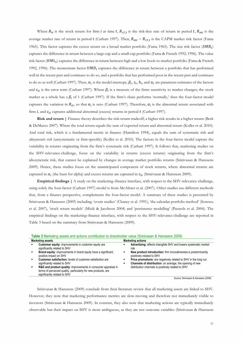
Empirical findings | A study on the marketing–finance interface, with respect to the SHV-relevance-challenge,

using solely the four-factor (Carhart 1997) model is from McAlister et al. (2007). Other studies use different methods

that, from a finance perspective, complements the four-factor model. A summary of these studies is presented by

Srinivasan & Hanssens (2009) including: ‘event studies’ (Chaney et al. 1991), ‘the calendar portfolio method’ (Sorescu

et al. 2007), ‘stock return models’ (Mizik & Jacobson 2004) and ‘persistence modelling’ (Pauwels et al. 2004). The

empirical findings on the marketing–finance interface, with respect to the SHV-relevance-challenge are reported in

Table 3 based on the summary from Srinivasan & Hanssens (2009).

Table 3 Marketing assets and actions contribution to shareholder value (Srinivasan & Hanssens 2009) Marketing assets Marketing actions § Customer equity: improvements in customer equity are

significantly related to SHV § Brand equity: improvements in brand equity have a significant,

positive impact on SHV § Customer satisfaction: levels of customer satisfaction are

significantly related to SHV § R&D and product quality: improvements in consumer appraisal in

terms of perceived quality, particularly for new products, are significantly related to SHV

§ Advertising: affects intangible SHV and lowers systematic market risk

§ New product introduction: firm innovativeness is predominantly positively related to SHV

§ Price promotions: are negatively related to SHV in the long run § Channels of distribution: on average, the opening of new

distribution channels is positively related to SHV

Source: Srinivasan & Hanssens (2009)

Srinivasan & Hanssens (2009) conclude from their literature review that all marketing assets are linked to SHV.

However, they note that marketing performance metrics are slow-moving and therefore not immediately visible to

investors (Srinivasan & Hanssens 2009). In contrast, they also note that marketing actions are typically immediately

observable but their impact on SHV is more ambiguous, as they are not outcome variables (Srinivasan & Hanssens

32

2009). Srinivasan & Hanssens (2009) finally note that preliminary evidence suggests that changes in firm value drive

some marketing actions. Or in other words, they acknowledge that at times there is a reverse causality effect of

marketing actions (Srinivasan & Hanssens 2009). The ultimate evidence of marketing’s-SHV-relevance-challenge is

provided by the impact of marketing related exogenous variables in the four-factor model (Carhart 1997),

demonstrating how marketing related managerial actions contributes to SHV (Srinivasan & Hanssens 2009).

2.2.1 Customer-based valuation

“Customers are the central object for valuing a firm”

Gupta et al. (2004)

As has become clear previously, the marketing department is in charge of building the intangible assets. This

requires them to assesses and communicate the (incremental) value of those assets. Recently, a new stream of valuation

literature has emerged in marketing, making the individual customer the central object of analysis.

Customer-based valuation | According to Schulze et al. (2012) CBV is a concept that values firms based on

information about their customer base. In addition, Gupta et al. (2004) argue that CBV is the term that describes all

approaches in which customers are the central object for valuing a firm. The premise of CBV in valuing the current

and future customer base of a firm is simple (Gupta et al. 2004). If the growth in number of customers can be

forecasted accurately, then the CLV framework can estimate the long-term value of a customer (Gupta & Lehmann

2003). CBV provides a good alternative approach for the forecast of future CFs of a firm (Gupta et al. 2004). Especially

in the situation where a firm has negative CFs, such that the DCF valuation method can’t be applied (Gupta et al.

2004; Koller et al. 2010). Or the situation in which a firm has no earnings such that the traditional P/E (price/earnings)

ratio can’t be applied either (Gupta et al. 2004; Koller et al. 2010). In addition, CBV can provide useful insights and

guidelines to investors, given that the firm’s overall value stems to a large extent from its customer base (Hogan et al.

2002; Kim et al. 1995). CBV has even found its way into investment banking, which is the industry that is specialized

in valuation (Gupta et al. 2006). In this example the investment banking department of Credit Suisse based a valuation

case largely on the estimation of CLV (Gupta et al. 2006). In essence this valuation case was about forecasting the

number of new customers and the future parameters of a CLV model (Gupta et al. 2006).

Marketing studies on customer-based valuation | Various marketing studies with regards to CBV have been

conducted. Libai, Muller & Peres (2009) and Rust et al. (2004) compare the value of current and future customers

against SHV. Kumar & Shah (2009) regress measures of CE on the share price of firms. The best-known example of

a CBV study is the one by Gupta et al. (2004). Their CBV approach was based on publicly available information of

five firms to estimate the after-tax value of the customer bases (Gupta et al. 2004). Their results show that the sum of

CLVs approximates market value of three firms very well (Gupta et al. 2004). For two firms total CLV is significantly

below their market values (Gupta et al. 2004). However, the results suggest either that they have unaccounted for

growth opportunities or that the market overvalued both firms (Gupta et al. 2004).

Customers as assets | “Customers have become the ultimate scarce resource” (Peppers & Rogers 2005), and

are the most important intangible asset of a firm (Gupta & Lehmann 2003). Lev (2001) has shown that in the US the

500 largest corporations have a market value of almost six times their book value; underlining again the importance of

intangible assets. As a result, a wide consensus has emerged around the importance of customers as assets (Gupta &

Lehmann 2003; Seybold 2001). Nevertheless, investors still mainly use traditional financial approaches where they

33

implicitly capitalize R&D expenditures, but continue to treat marketing and customer acquisition as an expense

(Demers & Lev 2001). In CBV customers are treated as assets, so that customer related (marketing) expenditures are

treated as investments (Gupta 2009). Therefore, investor’s need to know more about the intangible assets of a firm

(Gupta & Lehmann 2003). As a consequence, it is becoming increasingly important to value and manage customers

properly (Gupta & Lehmann 2003). According to Seybold (2001), this follows logically as a next step in the already

widely accepted importance of a customer-centric firm. However, the acceptance of customers recognized as assets is

negatively impacted by the requirements of extensive data and complex modeling (Gupta & Lehmann 2003).

Customer life time value concept | The fundamental building block for CBV of firms is the CLV concept,

developed and discussed in marketing literature (Gupta 2009). It is defined as the PV (Berk & DeMarzo 2007) of all

future CFs obtained during the relationship of a customer with the firm (Getz & Thomas 2001; Rust et al. 2001). CLV

has emerged as an important metric to manage and grow customers, and has gained the attention of senior executives

(Gupta 2009) and investors (Jain & Singh 2002) due to its link to SHV. Its acceptance in the boardroom stems from

its intuitive methodology very similar to DCF valuation, with two key differences (Gupta & Lehmann 2006). First, as

the name implies CLV is estimated at the individual customer level (Gupta & Lehmann 2006), where its acceptance

and use of it in customer management is driven by the ‘individual-aspect’ (Gupta & Lehmann 2006). Second, CLV

explicitly accounts for the possibility of customer defection (Gupta & Lehmann 2006). However, there have been few

attempts to capture a firm’s option value (Smit & Trigeorgis 2004), in the development of theoretical CLV models,

even though a firm’s option value often accounts for a large portion of total value (Gupta and Lehmann 2006; Koller

et al. 2010; Smit & Trigeorgis 2004). Gupta and Lehmann (2006) suggest that finance literature may be useful in further

developing such CLV models. For now, the proposed CLV models do not capture the entire market value of a firm,

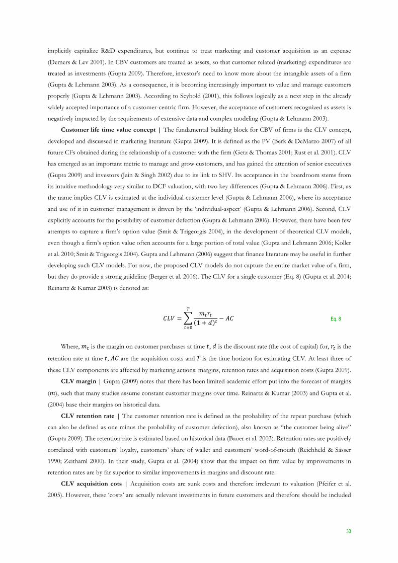
but they do provide a strong guideline (Berger et al. 2006). The CLV for a single customer (Eq. 8) (Gupta et al. 2004;

Reinartz & Kumar 2003) is denoted as:

B83 =

j(%(

1 + / (− 9B

k

(lm

Eq. 8

Where, j( is the margin on customer purchases at time ', / is the discount rate (the cost of capital) for, %( is the

retention rate at time ', 9B are the acquisition costs and : is the time horizon for estimating CLV. At least three of

these CLV components are affected by marketing actions: margins, retention rates and acquisition costs (Gupta 2009).

CLV margin | Gupta (2009) notes that there has been limited academic effort put into the forecast of margins

(j), such that many studies assume constant customer margins over time. Reinartz & Kumar (2003) and Gupta et al.

(2004) base their margins on historical data.

CLV retention rate | The customer retention rate is defined as the probability of the repeat purchase (which

can also be defined as one minus the probability of customer defection), also known as “the customer being alive”

(Gupta 2009). The retention rate is estimated based on historical data (Bauer et al. 2003). Retention rates are positively

correlated with customers’ loyalty, customers’ share of wallet and customers’ word-of-mouth (Reichheld & Sasser

1990; Zeithaml 2000). In their study, Gupta et al. (2004) show that the impact on firm value by improvements in

retention rates are by far superior to similar improvements in margins and discount rate.

CLV acquisition cots | Acquisition costs are sunk costs and therefore irrelevant to valuation (Pfeifer et al.

2005). However, these ‘costs’ are actually relevant investments in future customers and therefore should be included

34

in valuation (Gupta 2009). Though, improvements in acquisition costs have the smallest impact on firm value, among

the other CLV components (Gupta et al. 2004).

CLV horizon | Assumptions on the time horizon in CLV are determined to some extent by the product category

(Gupta 2009). Several assumptions have been used in studies. Reinartz & Kumar (2000) and Thomas (2001) use an

expected customer lifetime, Gupta et al. (2004); Fader, Hardie & Lee (2005) use an infinite time horizon.

CLV growth | Assuming that margins (j) and retention rates (%) are constant over time and the time horizon

is infinite and adding an extra growth rate (0) representing ‘acquisition growth per existing customer’, then CLV

simplifies to (Gupta & Lehmann 2003; 2006; Gupta et al. 2004) (Eq. 9):

B83 =

j%(

1 + / ((1 + 0) − 9B = j

%

1 + / − %(1 + 0) − 9B

n

(lm

Eq. 9

This is a simple CLV premise where the margin (j) is multiplied by a multiple (%/(1 + / − %) ∗ (1 + 0)), where

(%) is the retention rate, (/) the discount rate, times a growth rate (0) minus the acquisition costs (9B) for new

customers. This equation (Eq. 9) is the foundation of CBV that can be used for firm valuation (Gupta et al. 2004).

Customer equity | CE is defined as the sum of all CLVs and has emerged as a key metric to manage and grow

customers (Schulze et al. 2012). This concept is intrinsically related with the firm valuation concept as both are two

versions of the PV rule (Berk & DeMarzo 2007) of expected future CFs (Srinivasan & Hanssens 2009). This overlap

with finance makes marketing financially more relevant and accountable (Schulze et al. 2012). This is demonstrated by

Gupta & Lehmann (2003) and Gupta et al. (2004), as their estimated CE in these studies approximate the market value

of three out of five firms very well. Although CE does not capture all the sources of market value for a firm, it does

provide a strong guideline (Gupta & Lehmann 2003). Thus, the following is expected:

H2: CE and share price are positively correlated.

Gupta & Lehmann (2003) and Gupta et al. (2004) also show the relative impact of similar improvements between

the CE drivers. They find among others that a 100 basis points improvement in retention rate results in a 5% increase

of CE (Gupta & Lehmann 2003; Gupta et al. 2004). Thus, the following is expected:

H3: Improvements in the retention rate affects CE.

Customer equity to shareholder value | Schulze et al. (2012) incorporate valuation theory in their CE model,

in order to account for the effect of NOA and debt on CE in order to obtain SHV (Damodaran 2006; Koller et al.

2010). They propose the following adjustment to CE (Eq. 10):

123 = =YHM'Z[FGHI = B= + 569 − \I]' Eq. 10


H4: The EV estimated by DCF valuation, approximates CE estimated by CE valuation.

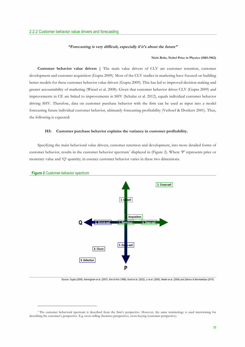
35

2.2.2 Customer behavior value drivers and forecasting

“Forecasting is very difficult, especially if it's about the future”

Niels Bohr, Nobel Prize in Physics (1885-1962)

Customer behavior value drivers | The main value drivers of CLV are customer retention, customer

development and customer acquisition (Gupta 2009). Most of the CLV studies in marketing have focused on building

better models for these customer behavior value drivers (Gupta 2009). This has led to improved decision making and

greater accountability of marketing (Wiesel et al. 2008). Given that customer behavior drives CLV (Gupta 2009) and

improvements in CE are linked to improvements in SHV (Schulze et al. 2012), equals individual customer behavior

driving SHV. Therefore, data on customer purchase behavior with the firm can be used as input into a model

forecasting future individual customer behavior, ultimately forecasting profitability (Verhoef & Donkers 2001). Thus,

the following is expected:

H5: Customer purchase behavior explains the variance in customer profitability.

Specifying the main behavioral value drivers, customer retention and development, into more detailed forms of

customer behavior, results in the customer behavior spectrum7 displayed in (Figure 2). Where ‘P’ represents price or

monetary value and ‘Q’ quantity; in essence customer behavior varies in these two dimensions.

Figure 2 Customer behavior spectrum

Source: Gupta (2009), Keiningham et al. (2007), Kim & Kim (1999), Knott et al. (2022), Li et al. (2005), Neslin et al. (2006) and Zakirov & Momtselidze (2015)

7 The customer behavioral spectrum is described from the firm’s perspective. However, the same terminology is used intertwining for

describing the customer’s perspective. E.g. cross-selling (business perspective), cross-buying (customer perspective).

1. Retention

2. Cross-sell

3. Up-sell

4. Deep-sell

7. Acquisition

6. Shrink-sell

5. Down-sell8. Churn

9. Defection

Q

P

36

Customer behavior value driver 1: retention | Keiningham et al. (2007) define customer retention as follows:

“the customers’ stated continuation of a business relationship with the firm.” Customer retention has a large impact

on firm profitability (Reichheld & Sasser 1990) and firm value (Gupta et al. 2004). Thus, the following is expected:

H6: There is a positive relation between retention and customer profitability.

Customer behavior value driver 2: cross-sell | Li et al. (2005) define cross-sell (or from the customer

perspective: cross-buying) as follows: “the practice of selling additional products or services to existing customers.”

Cross-sell is of high importance in CBV (Donkers et al. 2007), it mainly drives ROIs (Knott et al. 2002) and improves

margins (Gupta 2009). As a result, firms in many industries have put the highest strategic priority to cross-selling (Li

et al. 2005). Thus, the following is expected:

H7: There is a positive relation between cross-sell and customer profitability.

Customer behavior value driver 3: up-sell | Kim & Kim (1999) define up-sell (or from the customer

perspective: up-buying) as follows: “the firms attempt to sell a similar but more expensive version of the same services

or products.” Up-selling is an important component of CLV (Kim & Kim 1999) and improves margins (Gupta 2009).


H8: There is a positive relation between up-sell and customer profitability.

Customer behavior value driver 4: deep-sell | Zakirov & Momtselidze (2015) define deep-sell (or from the

customer perspective: deep-buying) as follows: “the attempt to let customers increase their usage of the services and

products they currently have.” Thus, the following is expected:

H9: There is a positive relation between deep-sell and customer profitability.

The behaviors cross-sell, up-sell and deep-sell imply the existence of a counterpart in the customer behavior

spectrum. The following types of customer behavior are exact opposites and are based on economic reasoning within

the described theoretical framework thus far.

Customer behavior value driver 5: down-sell | Down-sell (or from the customer perspective: down-buying)

can be perceived as the counterpart of customer up-sell; it follows that it can be defined as: ‘the firm selling less

expensive version of the same services or products.’ Thus, the following is expected:

H10: There is a negative relation between down-sell and customer profitability.

Customer behavior value driver 6: shrink-sell | Shrink-sell (or from the customer perspective: shrink-buying)

can be perceived as the counterpart of customer deep-sell; it follows that it can be defined as: ‘the firm selling less of

the same product or service to the same customer.’ Thus, the following is expected:

H11: There is a negative relation between shrink-sell and customer profitability.

37

The types of customer behavior discussed so far are more specified subtypes of both retention and development.

In essence these types come down to the fact that the customer is retained in the subsequent period, just that it has

changed its behavior in terms of ‘quantity’ (Q) or ‘monetary value’ (P) or a combination both. The following (and last)

types of customer behavior discussed, are independent customer behavior events within the spectrum.

Customer behavior value driver 7: acquisition | Gupta (2009) defines customer acquisition as follows: “the

first-time purchase by new or lapsed customers.” Customer acquisition has an important impact on long-term

profitability of the firm (Villanueva et al. 2008) and represents an important investment with effect on the future

retention rate (Thomas 2001). Moreover, Schulze et al. (2012) show that it affects SHV more than customer retention.

However, Reinartz et al. (2005) mention that firms poorly understand the underlying linkage between acquisition and

the long-term impact on profitability. Thus, the following is expected:

H12: There is a positive relation between acquisition and customer profitability.

Customer behavior value driver 8: churn | Neslin et al. (2006) define customer churn as follows: “the moment

a customer does not stay with a certain product or service of the firm8.” In their study they conclude that customer

churn has a negative impact on CLV. Thus, the following is expected:

H13: There is a negative relation between churn and customer profitability.

Customer behavior value driver 9: defection | Gupta (2009) defines customer defection as follows: “a

customer that is lost for good.” In addition, he notes that some researchers consider customer defection as ‘switching

to competitors’ as transient, or ‘always a share.’ The probability of customer defection is explicitly part of CLV (Gupta

2009). Thus, the following is expected:

H14: There is a negative relation between defection and customer profitability.

When observing a single customer’s behavior during a certain period, a variety of purchase behavior combinations

can occur at once. In the most ‘extreme’ scenario all types can occur in the same time, apart from acquisition and

defection as these are isolated events. Multi-purchase behavior is induced by at least two factors. In the first place this

is due to multi-brand, multi-product and multi-segment. Then, cross-sell as a common highest strategic priority (Li et

al. 2005) functions as a catalyst for ‘multi-purchase-behavior’ and encourages customers to be more exposed to firm

products, which drives general purchase-behavior activity. The impact of both factors is supported by findings from

Donkers et al. (2007) on purchase behavior between two periods among several products within one insurance firm

(Donkers et al. 2007). They find high correlations among purchased products for subsequent years, especially on the

diagonal (Donkers et al. 2007). This indicates that a product is repurchased and implicitly drives retention (Donkers et

al. 2007). But they also find high correlations between different products, indicating cross-sell and or churn (Donkers

et al. 2007). Thus, the following is expected:

H15: Observed customer behavior affects future customer behavior.

8 The customer remains with the firm purchasing other products or services, but simply ends for example a product in a certain product

category.

38

2.2.3 Customer brand choice behavior and forecasting

“Through the years, customers may come and go, but strong brands will endure”

Leone et al. (2006)

Customers and brands are two sides of the same coin; they both improve the profitability of marketing within

the firm (Leone et al. 2006).

Brand equity | In addition to the CE metric, marketing has developed another equity metric for the value

measurement of its other major intangible asset: brands (Doyle 2000). Together with other marketing intangibles brand

equity accounts on average for 75% of a firm’s value (Doyle 2000). Keller (1993) defines customer based brand equity

as: “the differential effect of brand knowledge on consumer response to the marketing of the brand.” This definition

implies that in the end customers drive a brand’s success. The firm’s marketing department develops brands for

customers (Bick 2009) to be attracted, to be reminded (Lemon et al. 2001) and to be connected emotionally to the firm

(Lemon et al. 2001; Leone et al. 2006). Brands represent value to customers (Aaker 1996). As a result, this drives

customer loyalty and price premiums driving incremental CFs (Leone et al. 2006), hence SHV (Bick 2009; Koller et al.

2010).

Brand choice behavior | Customers need and value brands (Leone et al. 2006). However, in the end a brand is

only as good as the customers it attracts (Leone et al. 2006). The associations a customer has with a brand drives the

brand experience, affecting customer satisfaction and customer loyalty (Brakus et al. 2009). As loyalty goes down a

customer is more likely to switch between brands of which it might derive utility from switching itself and the new

brand choice (McAlister & Pessemier 1982; Van Oest & Franses 2005). Ultimately, the customer brand-switching is

related to individual customer brand choice behavior (Van Oest & Franses 2005). From a theoretical perspective

customer brand choice behavior is complementary to the customer behavior value driver spectrum (Figure 2), as it

moderates a customer’s movement within the spectrum. Thus, the following is expected:

H16: Customer brand choice affects customer behavior.

H17: Customer brand choice affects customer profitability.

2.2.4 Customer characteristics, relationship age, share of wallet and forecasting

Customer characteristics or socio-demographics, are important predictors (Kamakura et al. 1991). In addition to

the traditional variables (e.g. income, age, education, household composition, gender, risk attitude, social class, etc.),

the family lifecycle is a good predictor as well (Antonides & van Raaij 1998). Customer characteristics are linked to

customer needs (Engel et al. 1995) and customer needs drive the purchase decision process (Hauser & Urban 1986).

In addition, Verhoef & Donkers (2001) note that: “as there is hardly ever complete information on needs available,

customer characteristics relating to tastes and needs can be used instead.” It follows that, to a certain extent customer

characteristics drive the movements within the customer behavior value driver spectrum (Figure 2). Thus, the following

is expected:

H18: Customer characteristics affect customer behavior.

39

As customer characteristics are indirectly linked to customer purchase behavior, it follows that customer

characteristics are linked to customer profitability. Thus, the following is expected:

H19: Customer characteristics affect customer profitability.

Relationship age | The customer’s length of the relationship has a moderating effect on loyalty (Cooil et al.

2007) and is a good predictor for retention probabilities (Donkers et al. 2007). The relationship of the firm with the

customer evolves over time, creating a bond between them (Cooil et al. 2007). As a result, this decreases the probability

of a customer’s defection (Anderson & Sullivan 1993), and creates satisfaction that drives customer loyalty (Anderson

& Weitz 1989). The cumulative effect of the customer journey with the firm affects the customer’s entire judgement

of its relationship (Kalwani & Narayandas 1995). So, when the length of a customer relationship ages, movements in

satisfaction have less impact on loyalty (Homburg et al. 2003). In addition, switching costs tend to increase when the

relationship length increases (Cooil et al. 2007). Thus, the following is expected:

H20: Relationship age affects customer purchase behavior.

H21: There is a positive relation between relationship age and customer profitability.

Share of wallet | Keiningham et al. (2007) define customer SOW as follows: “the stated percentage of total

spending on products or services held at the firm with respect to the total capacity of the customers’ wallet.” In

addition, it measures customer loyalty behavior (Bowman et al. 2000; Bowman & Narayandas 2004; Jones & Sasser

1995). However, measures of loyalty are forward looking, where SOW just summarizes the current situation in a single

metric (Oliver 1999). Improvements in customers’ SOW results in greater financial impact than customer retention

(Keiningham et al. 2007). In combination with retention improvements, this results in ten-times greater value to a firm

than customer-retention improvements solely (Coyles & Gokey 2005). Thus, the following is expected:

H22: Share of wallet affects customer purchase-behavior.

H23: There is a positive relation between share of wallet and customer profitability.

2.3 Conceptual model

The conceptual model derived from theory is displayed in Figure 3, presenting two value driver concepts in

valuation. The concept above the blue line is in essence the value driver model derived from DCF valuation theory.

Below the line, is a value driver model based on customer behavior derived from both CBV and DCF theory. Both

concepts are two sides of the same coin, having only one value driver in common: the firm’s marketing-strategy,

resulting from boardroom strategy development. A well-balanced marketing mix execution then drives the chain of

value drivers for both concepts, driving the product-market performance of the firm. The conceptual model

emphasizes the differences in value driver’s origin. For the DCF value driver concept this is more ‘product-centric’

oriented, where for the customer behavior based value driver concept has a solely ‘customer-centric’ orientation. Both

concepts aim to forecast future CFs based on the changes in value drivers. The systematic risk surrounding future CFs

40

needs to be taken into account by discounting future CFs at the firm’s WACC representing the COC. The level of

WACC is essentially a consequence of the firm’s strategy. Ultimately, after some financial adjustments, both value

driver concepts are expected to result similar SHV estimates. In addition, estimated CE (including NOA) is expected

to be of a same level as the EV. Finally, there is a feedback loop of SHV to strategy. This line is left out on purpose

from the conceptual model, as it is out of the scope of this study. Nevertheless, it is important to underline the

continuous process underlying this conceptual model.

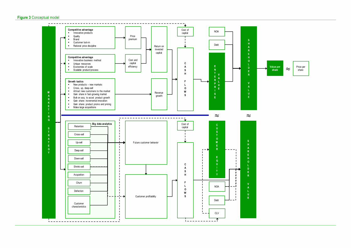
Figure 3 Conceptual model

Big data analytics

SHAREHOLDER

VALUE

Cost of capital

Price premium

MARKETING

STRATEGY

Competitive advantage§ Innovative products§ Quality§ Brand§ Customer lock-in§ Rational price discipline

Competitive advantage§ Innovative business method§ Unique resources§ Economies of scale§ Scalable product/process

Cost and capital

efficiencyCASH

FLOWS

Growth tactics§ New products – new markets§ Cross, up, deep-sell§ Attract new customers to the market§ Gain share in fast-growing market§ Bolt-on acq. to accel. product growth§ Gain share: incremental innovation§ Gain share: product promo and pricing§ Make large acquisitions

Return on invested capital

Revenue growth

Value per share

Price per share≈

Future customer behavior

CLV

CUSTOMER

EQUITY

Customer profitability

Customer characteristics

Cross-sell

Up-sell

Deep-sell

Down-sell

Shrink-sell

Acquisition

Churn

Defection

CASH

FLOWS

ENTERPRISE

VALUE

≈

SHAREHOLDER

VALUE

≈Retention

Debt

NOA

Cost of capital

Debt

NOA

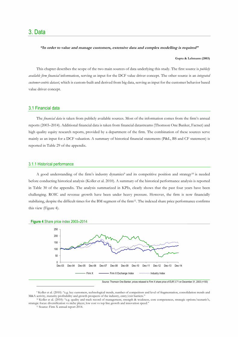
3. Data

“In order to value and manage customers, extensive data and complex modelling is required”

Gupta & Lehmann (2003)

This chapter describes the scope of the two main sources of data underlying this study. The first source is publicly

available firm financial information, serving as input for the DCF value driver concept. The other source is an integrated

customer-centric dataset, which is custom-built and derived from big data, serving as input for the customer behavior based

value driver concept.

3.1 Financial data

The financial data is taken from publicly available sources. Most of the information comes from the firm’s annual

reports (2003–2014). Additional financial data is taken from financial datastreams (Thomson One Banker, Factset) and

high quality equity research reports, provided by a department of the firm. The combination of these sources serve

mainly as an input for a DCF valuation. A summary of historical financial statements (P&L, BS and CF statement) is

reported in Table 29 of the appendix.

3.1.1 Historical performance

A good understanding of the firm’s industry dynamics9 and its competitive position and strategy10 is needed

before conducting historical analysis (Koller et al. 2010). A summary of the historical performance analysis is reported

in Table 30 of the appendix. The analysis summarized in KPIs, clearly shows that the past four years have been

challenging. ROIC and revenue growth have been under heavy pressure. However, the firm is now financially

stabilizing, despite the difficult times for the BM segment of the firm11. The indexed share price performance confirms

this view (Figure 4).

Figure 4 Share price index 2003–2014

Source: Thomson One Banker, prices rebased to Firm X share price of EUR 3.71 on December 31, 2003 (=100)

9 Koller et al. (2010): “e.g. key customers, technological trends, number of competitors and level of fragmentation, consolidation trends and

M&A activity, maturity profitability and growth prospects of the industry, entry/exit barriers.” 10 Koller et al. (2010): “e.g. quality and track record of management, strength & weakness, core competences, strategic options/scenario’s,

strategic focus: diversification vs niche player, low cost vs top line growth and innovation speed.” 11 Source: Firm X annual report 2014.

0

50

100

150

200

250

Dec-14Dec-13Dec-12Dec-11Dec-10Dec-09Dec-08Dec-07Dec-06Dec-05Dec-04Dec-03

Firm X Firm X Exchange Index Industry Index

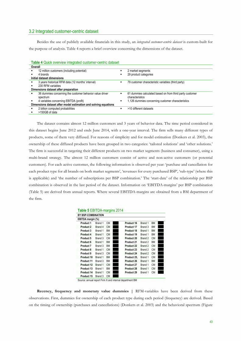
43

3.2 Integrated customer-centric dataset

Besides the use of publicly available financials in this study, an integrated customer-centric dataset is custom-built for

the purpose of analysis. Table 4 reports a brief overview concerning the dimensions of the dataset.

Table 4 Quick overview integrated customer-centric dataset Overall § 12 million customers (including potential) § 4 brands

§ 2 market segments § 29 product categories

Initial dataset dimensions § 3 years historical RFM data (12 months’ interval) § 230 RFM variables

§ 79 customer characteristic variables (third party)

Dimensions dataset after preparation § 36 dummies concerning the customer behavior value driver

spectrum § 4 variables concerning EBITDA (profit)

§ 61 dummies calculated based on from third party customer characteristics

§ 1,126 dummies concerning customer characteristics Dimensions dataset after model estimation and solving equations § 2 billion computed probabilities § >150GB of data

§ >10 different datasets

The dataset contains almost 12 million customers and 3 years of behavior data. The time period considered in

this dataset begins June 2012 and ends June 2014, with a one-year interval. The firm sells many different types of

products, some of them very diffused. For reasons of simplicity and for model estimation (Donkers et al. 2003), the

ownership of these diffused products have been grouped in two categories: ‘tailored solutions’ and ‘other solutions.’

The firm is successful in targeting their different products on two market segments (business and consumer), using a

multi-brand strategy. The almost 12 million customers consist of active and non-active customers (or potential

customers). For each active customer, the following information is observed per year: ‘purchase and cancellation for

each product type for all brands on both market segments’, ‘revenues for every purchased BSP’, ‘sub-type’ (where this

is applicable) and ‘the number of subscriptions per BSP combination.’ The ‘start-date’ of the relationship per BSP

combination is observed in the last period of the dataset. Information on ‘EBITDA-margins’ per BSP combination

(Table 5) are derived from annual reports. Where several EBITDA-margins are obtained from a BM department of

the firm.

Table 5 EBITDA-margins 2014 BY BSP-COMBINATION EBITDA margin (%)

Product 1 Brand 1 CM XX % Product 16 Brand 1 BM XX % Product 2 Brand 4 CM XX % Product 17 Brand 3 BM XX % Product 3 Brand 1 BM XX % Product 18 Brand 1 BM XX % Product 4 Brand 1 CM XX % Product 19 Brand 1 BM XX % Product 5 Brand 3 CM XX % Product 20 Brand 2 CM XX % Product 6 Brand 1 BM XX % Product 21 Brand 2 BM XX % Product 7 Brand 3 BM XX % Product 22 Brand 2 CM XX % Product 8 Brand 1 CM XX % Product 23 Brand 2 CM XX % Product 9 Brand 3 CM XX % Product 24 Brand 2 CM XX % Product 10 Brand 1 BM XX % Product 25, Brand 1 CM XX % Product 11 Brand 3 BM XX % Product 26 Brand 1 BM XX % Product 12 Brand 1 CM XX % Product 27 Brand 1 CM XX % Product 13 Brand 1 BM XX % Product 28 Brand 1 CM XX % Product 14 Brand 1 CM XX % Product 29 Brand 1 CM XX % Product 15 Brand 3 CM XX %

Source: annual report Firm X and internal department BM

Recency, frequency and monetary value dummies | RFM-variables have been derived from these

observations. First, dummies for ownership of each product type during each period (frequency) are derived. Based

on the timing of ownership (purchases and cancellations) (Donkers et al. 2003) and the behavioral spectrum (Figure

44

2) 9 behavioral dummies (recency) have been derived. These behavioral dummies are derived based on the transition

during the periods 2012–2013 and 2013–2014. A customer’s total EBITDA contribution (monetary value), is derived

as the sum of: ownership dummies for each product type times the product specific EBITDA-margin.

Relationship age dummies | The relationship age per product in the customer’s portfolio is observed for the

last period (2014). The longest relationship among the customer’s portfolio is taken for the derivation of 11 dummies

indicating the relationship age.

Customer characteristic dummies | Variables on customer characteristics (socio-demographics) complement

the dataset. These variables originate from commercial third-party sources,12 and contain information on an aggregated

business and household level. For each individual customer in the dataset (consumer and business; active and potential-

customers), these variables are observed in the last period (2014) of the dataset. These variables may be aggregated on

the location, household or business level. Customer characteristics have predictive power (Verhoef & Donkers 2001).

In addition, these variables bridge the ‘data-gap’ in between active customers and non-active customers (potential

customers). Hence, there is no purchase behavior data available for non-active customers. As a first impression of

predictability, Pearson correlation coefficients between the customer characteristics (before being recoded into

dummies) and EBITDA (2013 and 2014) are reported in Table 6. These variables have been selected from a broader

list of variables by economic reasoning. There are two significant and relatively substantial correlations (≥.10) with

regards to the ‘number of employees.’ Indicating that the size of a firm is positively related to total EBITDA. It is

expected that, especially after recoding into dummies, more variables will have substantial predictive power. All

customer characteristics have been recoded, resulting in 1,176 dummy variables.

Share of wallet dummies | Combining observed RFM-variables with customer characteristics enables the

computation of a customer’s SOW. The formula (Eq. 11) for calculating SOW for a CM customer ! at time " (June

2014) (Cooil et al. 2007) is:

#$%&'(,*

=,-./0,1230,1

Eq. 11

Where ,-./0,1 is customer’s ! annual revenues with the firm at time " and 230,1 is its aggregated average annual

fiscal income. For a BM customer ! the SOW concerning Firm X industry’s related products and services at time " is

defined (Eq. 12) (Gartner IT Key Metrics Data 2012) as:

#$%4'(5,*

=,-./06,18(#06,1)

Eq. 12

Here ;is the type industry where the BM customer is active in, 8(#06,1) is its estimated annual industry related

spending at time ". Then the estimated annual industry related spending (8(#06,1)) is derived as follows (Eq. 13):

8 #06,1 = <=06,1 ∗ -,-./06,1 Eq. 13

12 SIZO provides business related information (www.sizo.com). Mosaic provides household related information (www.experian.nl/mosaic).

45

Table 6 Pearson correlations of third party customer characteristics and EBITDA 2013–2014 (r-coefficient) EBITDA EBITDA Customer characteristics 2013 2014 Customer characteristics 2013 2014

1 Number of SIZO BM .01** .01** 36 House type CM .01** .01** 2 Number of ultimate parents BM .01** .01** 37 Tenure CM .00** .00** 3 Special location (indicator) HYB -.00** -.00** 38 Number of moves CM .00 .00 4 Complex for demolition (indicator) HYB -.01** -.01** 39 Last move CM -.00** -.00** 5 Competitor 1 available on location (indicator) HYB .00* .00 40 Business HYB -.01** -.01** 6 Competitor 2 available on location (indicator) HYB .00 .00 41 Density surrounding addresses HYB .00 .00 7 Competitor 3 available on location (indicator) HYB .00 .00 42 Degree of urbanity HYB .00 .00 8 Competitor 4 available on location (indicator) HYB .00 .00 43 Number of residents CM .00 .00 9 Years since business establishment BM -.01** -.01** 44 Number of men CM .00 .00

10 Importing business (indicator) BM .01** .01** 45 Number of women CM .00 .00 11 Exporting business (indicator) BM .01** .01** 46 Percentage age 0-5 CM .00 .00 12 Mother company (indicator) BM .02** .02** 47 Percentage age 5-25 CM .00 .00 13 Number of employees BM .15** .15** 48 Percentage age 25-45 CM .00 .00 14 Number of employees in concern BM .02** .02** 49 Percentage age 45-65 CM .00 .00 15 Number of employees on concern location BM .19** .19** 50 Percentage age ≥65 CM .00 .00 16 Business complex (indicator) BM .02** .02** 51 Percentage nonwestern immigrant CM -.01** -.01** 17 Number of parts in concern BM .01** .01** 52 Number of total private households CM .00 .00 18 Score decision making unit (DMU) BM .01** .01** 53 Percentage one person households CM .00 .00 19 Score decision making unit location (DMU) BM .03** .03** 54 Percentage more persons households without children CM .00 .00 20 Months since last annual report BM .02** .02** 55 Percentage more persons households with children CM .00 .00 21 Consolidated results (category) BM .04** .04** 56 Average household size CM .00 .00 22 Revenues BM .07** .07** 57 Number of housing CM .00 .00 23 Consolidated revenues BM .06** .06** 58 Average house value EUR000 CM .00 .00 24 Special location type (category) BM -.00* -.00* 59 Average fiscal income EUR/month CM .00* .00 25 Mosaic group description (category) CM -.00** -.00** 60 Percentage low income CM .00 .00 26 Segment type (category) CM .00 .00 61 Percentage high income CM .01 .00 27 Age household CM .00* .00** 62 Percentage benefit recipients CM .00 .00 28 Age oldest child in household CM .06** .05** 63 Percentage entrepreneur CM -.00 .00 29 Household size CM .00** .00** 64 SBI segment description BM .01** .01** 30 Marital status CM .00** .00** 65 Percentage on industry related spending (Gartner) BM -.01 -.00 31 Average income (category) CM .01** .01** 66 NACE description BM .01** .01** 32 Level of education CM .00** .00** 67 Main or sub (indicator) BM .00 .00 33 Work situation CM .00 .00 68 Legal entity type BM -.00** -.00** 34 Number of cars household CM .00** .00** 69 Relationship to concern BM .02** .02** 35 Number of children CM .01** .02** 70 Code ZZP type BM -.01** -.01** **: p<0.01, *: p<0.05

Where <=06,1 is the Gartner industry related percentage spending for customer ! in industry ; at time " and

-,-./06,1 is its reported annual revenue taken from the annual report customer ! in industry ; at time ". Finally, the

Gartner Percentage (<=06,1) (Eq. 14) for customer ! in industry ; at time " is calculated as:

<=06,1 =

#6,1?@-./6,1?@

Eq. 14

Where #6,1?@ is the total industry related spending per industry ; in the previous period "AB and -./6,1?@ are the

total revenues generated by this industry ; in the previous period "AB. The Gartner percentage on industry related

spending is available for many different industries. Based on industry descriptions in the customer dataset, coming

from third party sources, Gartner’s industry related percentage is linked to individual business customers.

3.2.1 Data availability

Five major internal and external factors have influenced the eventual shape and content of the integrated

customer-centric dataset.

46

Geographical definition | The first factor of influence is the geographical definition of the customers

represented in the dataset. The focus is on the home country activities of the firm,13 accounting for the vast majority

of revenues; about 80%14 of total revenues in 2014. The major brands positioned on its home market are: Brand 115,

Brand 216, Brand 317 and Brand 418 accounting for an estimated 75% of total revenues for the home market division.

As a result, the Brand 519 group (foreign division) and Brand 620 customers are out of the scope of the dataset.

Data architecture | The second factor of influence is the architecture of data within the firm. As a consequence,

there is no data available for the remaining home market labels: Brand 721, Brand 822 and Brand 923. Roughly estimated,

these labels represent at maximum just a few percent of total revenues in 2014. However, the firm does not disclose

any information on these brands. One explanation for the current data-architecture arises from talks with internal data-

specialists. Historical agreements at times of mergers and acquisitions left the acquired firm with a certain degree of

autonomy, such as data-ownership. This has resulted in situations where information sharing (customer data) is

executed on aggregated levels.

Data accessibility | The third factor of influence is the accessibility of customer data. The specialized analyst

team is limited to accessing customer data on the level of product ownerships. Analysis on e.g. web related activity of

customers is analyzed by another specialized team. Customer-service related activities are analyzed by yet another team.

In short, the firm has diffused teams across the brands and market segments that do not cooperate in sharing data or

conducting analysis. As a result, there is a limited data accessibility for analysts across the firm. The diffused data-

ownership across the firm, has limited the data availability for this study.

Regulation | The fourth factor of influence comes from regulation imposed by the regulation authority. It

follows that, the collection of the data is in compliance with these regulations. Two measures with major impact on

the data collection are: (1) restricted period of customer data storage, and (2) the use of customer specific data for

analysis purposes is forbidden. The last measure directly limits the amount of available variables in the dataset with

expected highly predictive capacity, as it was expected to contain detailed information on customer behavior.

Newly developed dataset | This dataset is the outcome of a first-time attempt within the firm, in developing

an integrated customer-centric view. Therefore, this dataset is a unique approach in bridging the analysis-gap in multi-

dimensional customer purchase-behavior (in a context of multi-segment, multi-brand and multi-product). As a result,

learnings from the development-process of this dataset serve as input in developing a dataset with even more

integration of data sources in the future.

Consequences | Two consequences emerge from the limitations surrounding the data. In the first place, the

almost 12 million active and non-active customers in the dataset are in fact unique locations. At the moment of

constructing the dataset it was impossible to build a dataset based on solely individual customers. For simplicity reasons

it is assumed24 that every unique location equals one unique customer. On average, in 88% of the cases there is an one-

to-one relation between the location and the customer as reported in Table 31 of the appendix. In the second place,

13 At the time of constructing the dataset, Firm X was in the process of selling foreign activities. 14 Source: Firm X annual report 2014. 15 Is the quality brand, providing their customers with value-added services (source: Firm X annual report 2014). 16 Is the brand serving the no frills segment (source: Firm X annual report 2014). 17 Is the high-end brand for the top of the market (source: Firm X annual report 2014). 18 Is the brand targeting youth (source: Firm X annual report 2014). 19 Is the brand that pursues a challenger strategy on a foreign market (source: Firm X annual report 2014). 20 Is the brand that provides national and international wholesale to third parties (source: Firm X annual report 2014). 21 Is the online brand with specific propositions (source: Firm X annual report 2014). 22 Is the low-cost brand for internationally oriented customers (source: Firm X annual report 2014). 23 Is the challenger brand that focusses on the SME segment (source: Firm X annual report 2014). 24 The assumption may influence the valuation outcome; as customer-behavior is not always observed for the individual, thus affecting the

profitability or CF forecast, hence value.

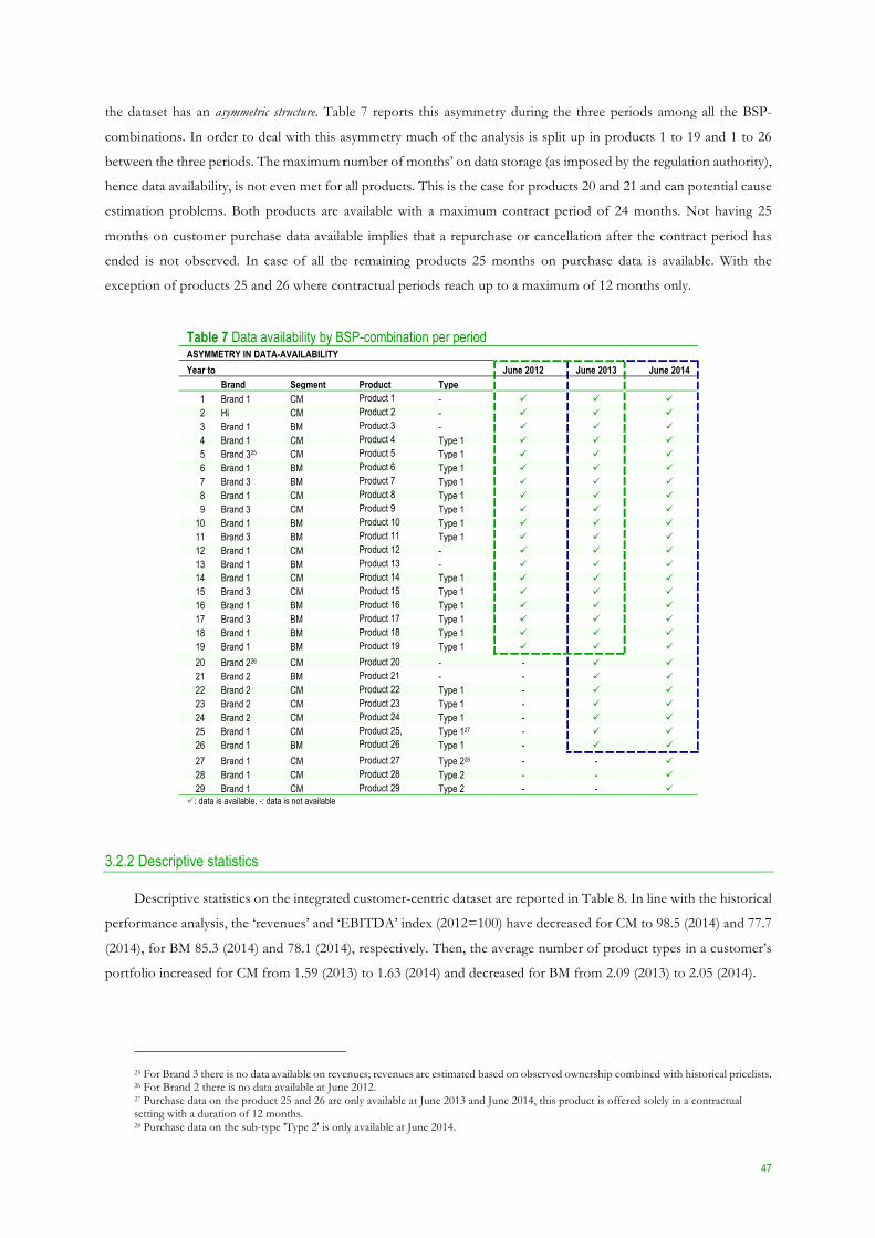
47

the dataset has an asymmetric structure. Table 7 reports this asymmetry during the three periods among all the BSP-

combinations. In order to deal with this asymmetry much of the analysis is split up in products 1 to 19 and 1 to 26

between the three periods. The maximum number of months’ on data storage (as imposed by the regulation authority),

hence data availability, is not even met for all products. This is the case for products 20 and 21 and can potential cause

estimation problems. Both products are available with a maximum contract period of 24 months. Not having 25

months on customer purchase data available implies that a repurchase or cancellation after the contract period has

ended is not observed. In case of all the remaining products 25 months on purchase data is available. With the

exception of products 25 and 26 where contractual periods reach up to a maximum of 12 months only.

Table 7 Data availability by BSP-combination per period ASYMMETRY IN DATA-AVAILABILITY Year to June 2012 June 2013 June 2014

Brand Segment Product Type 1 Brand 1 CM Product 1 - ü ü ü 2 Hi CM Product 2 - ü ü ü 3 Brand 1 BM Product 3 - ü ü ü 4 Brand 1 CM Product 4 Type 1 ü ü ü 5 Brand 325 CM Product 5 Type 1 ü ü ü 6 Brand 1 BM Product 6 Type 1 ü ü ü 7 Brand 3 BM Product 7 Type 1 ü ü ü 8 Brand 1 CM Product 8 Type 1 ü ü ü 9 Brand 3 CM Product 9 Type 1 ü ü ü

10 Brand 1 BM Product 10 Type 1 ü ü ü 11 Brand 3 BM Product 11 Type 1 ü ü ü 12 Brand 1 CM Product 12 - ü ü ü 13 Brand 1 BM Product 13 - ü ü ü 14 Brand 1 CM Product 14 Type 1 ü ü ü 15 Brand 3 CM Product 15 Type 1 ü ü ü 16 Brand 1 BM Product 16 Type 1 ü ü ü 17 Brand 3 BM Product 17 Type 1 ü ü ü 18 Brand 1 BM Product 18 Type 1 ü ü ü 19 Brand 1 BM Product 19 Type 1 ü ü ü

20 Brand 226 CM Product 20 - - ü ü 21 Brand 2 BM Product 21 - - ü ü 22 Brand 2 CM Product 22 Type 1 - ü ü 23 Brand 2 CM Product 23 Type 1 - ü ü 24 Brand 2 CM Product 24 Type 1 - ü ü 25 Brand 1 CM Product 25, Type 127 - ü ü 26 Brand 1 BM Product 26 Type 1 - ü ü

27 Brand 1 CM Product 27 Type 228 - - ü 28 Brand 1 CM Product 28 Type 2 - - ü 29 Brand 1 CM Product 29 Type 2 - - ü

ü: data is available, -: data is not available

3.2.2 Descriptive statistics

Descriptive statistics on the integrated customer-centric dataset are reported in Table 8. In line with the historical

performance analysis, the ‘revenues’ and ‘EBITDA’ index (2012=100) have decreased for CM to 98.5 (2014) and 77.7

(2014), for BM 85.3 (2014) and 78.1 (2014), respectively. Then, the average number of product types in a customer’s

portfolio increased for CM from 1.59 (2013) to 1.63 (2014) and decreased for BM from 2.09 (2013) to 2.05 (2014).

25 For Brand 3 there is no data available on revenues; revenues are estimated based on observed ownership combined with historical pricelists. 26 For Brand 2 there is no data available at June 2012. 27 Purchase data on the product 25 and 26 are only available at June 2013 and June 2014, this product is offered solely in a contractual setting with a duration of 12 months. 28 Purchase data on the sub-type 'Type 2' is only available at June 2014.

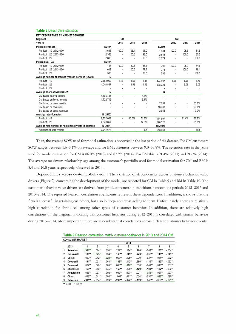
48

Table 8 Descriptive statistics KEY DESCRIPTIVES BY MARKET SEGMENT Segment CM BM Year to 2012 2013 2014 2012 2013 2014 Indexed revenues EURm EURm

Product 1-19 (2012=100) 1,693 100.0 96.4 96.0 1,934 100.0 95.5 81.5 Product 1-26 (2013=100) 2,353 - 100.0 98.5 2,646 - 100.0 85.3 Product 1-29 2,603 - - 100.0 2,274 - - 100.0

Indexed EBITDA EURm Product 1-19 (2012=100) 427 100.0 89.3 68.3 799 100.0 96.9 74.6 Product 1-26 (2013=100) 613 - 100.0 77.7 774 - 100.0 78.1 Product 1-29 518 - - 100.0 596 - - 100.0

Average number of product types in portfolio (RGUs) N Product 1-19 2,852,069 1.48 1.58 1.41 474,997 1.66 1.68 1.76 Product 1-26 4,040,857 - 1.59 1.63 598,325 - 2.09 2.05 Product 1-29 - - - - - - - -

Average share of wallet (SOW) N N CM based on avg. income 1,805,431 - - 1.6% - - - - CM based on fiscal. income 1,722,746 - - 3.1% - - - - BM based on cons. results - - - - 7,791 - - 33.8% BM based on revenues - - - - 16,433 - - 23.6% BM based on cons. revenues - - - - 2,956 - - 9.0%

Average retention rates N (2012) Product 1-19 2,852,069 - 86.0% 71.8% 474,997 - 91.4% 82.2% Product 1-26 4,040,857 - - 87.9% 598,325 - - 91.6%

Average max number of relationship years in portfolio N (2014) N (2014) Relationship age (years) 3,941,674 - - 8.4 543,961 - - 10.8

Then, the average SOW used for model estimation is observed in the last period of the dataset. For CM customers

SOW ranges between 1.6–3.1% on average and for BM customers between 9.0–33.8%. The retention rate in the years

used for model estimation for CM is 86.0% (2013) and 87.9% (2014). For BM this is 91.4% (2013) and 91.6% (2014).

The average maximum relationship age among the customer’s portfolio used for model estimation for CM and BM is

8.4 and 10.8 years respectively, observed in 2014.

Dependencies across customer-behavior | The existence of dependencies across customer behavior value

drivers (Figure 2), concerning the development of the model, are reported for CM in Table 9 and BM in Table 10. The

customer behavior value drivers are derived from product ownership transitions between the periods 2012–2013 and

2013–2014. The reported Pearson correlation coefficients represent these dependencies. In addition, it shows that the

firm is successful in retaining customers, but also in deep- and cross-selling to them. Unfortunately, there are relatively

high correlation for shrink-sell among other types of customer behavior. In addition, there are relatively high

correlations on the diagonal, indicating that customer behavior during 2012–2013 is correlated with similar behavior

during 2013–2014. More important, there are also substantial correlations across different customer behavior-events.

Table 9 Pearson correlation matrix customer-behavior in 2013 and 2014 CM CONSUMER MARKET 2014 2013 1 2 3 4 5 6 7 8 9 1 Retention .331** .084** .050** .224** .164** .286** -.245** .163** -.004** 2 Cross-sell .118** .025** .034** .166** .145** .243** -.062** .149** -.049** 3 Up-sell .059** .012** .022** .053** .106** .079** -.027** .034** -.032** 4 Deep-sell .191** .031** .061** .189** .142** .296** -.130** .132** -.022** 5 Down-sell .032** .040** .009** .003** .017** .038** -.041** .018** .031** 6 Shrink-sell .169** .052** .045** .160** .105** .129** -.109** .102** -.032** 7 Acquisition .056** .037** -.002** .082** .027** .027** -.056** .027** .027** 8 Churn .032** .041** .006** .001* .011** .024** -.035** .012** .020** 9 Defection -.395** -.054** -.024** -.239** -.074** -.139** .042** -.069** -.071** **: p<0.01, *: p<0.05

49

Table 10 Pearson correlation matrix customer-behavior in 2013 and 2014 BM BUSINESS MARKET 2014 2013 1 2 3 4 5 6 7 8 9 1 Retention .329** .033** .052** .136** .198** .311** -.279** .192** -.073** 2 Cross-sell .106** .012** .037** .135** .139** .171** -.057** .137** -.065** 3 Up-sell .054** .008** .043** .061** .092** .085** -.027** .039** -.036** 4 Deep-sell .184** .027** .061** .206** .169** .294** -.118** .153** -.090** 5 Down-sell .042** .023** .019** -.003* .039** .050** -.048** .032** .007** 6 Shrink-sell .157** .011** .048** .059** .131** .128** -.136** .120** -.033** 7 Acquisition .028** .004** -.010** -.046** -.012** -.014** -.044** -.005** .020** 8 Churn .033** .023** .011** -.011** .024** .031** -.043** .020** .013** 9 Defection -.368** -.037** -.021** -.179** -.091** -.160** .066** -.089** 0.002 **: p<0.01, *: p<0.05

Purchase rates | Descriptive statistics on purchase rates across product ownerships are reported in Table 32 of

the appendix. Customer defection in relation to purchase rates of the products is expected to decrease over time for

the retained customers. However, for 10 out of 26 products (2013–2014) these rates increase, indicating that the firm

is relatively successful at cross-selling. This is expected, since customers who purchase more products are more likely

to stay with the firm (Donkers et al. 2007).

Ownership correlations | An ownership correlations matrix of these products is reported in Table 33 of the

appendix. There are high correlations on the diagonal, so having a certain product type in 2013 is highly correlated

with having that same product in 2014. More important, there are also substantial correlations across different product

types. Both findings are in in accordance with Donkers et al. (2007).

4. Methodology

“Forecasting is very difficult, especially if it's about the future”

Niels Bohr (1885–1962), Nobel Prize in Physics

This chapter describes the different methods used for valuation. Both main methods, DCF and CBB valuation

aim to determine the level of SHV, but have a total different approach in forecasting key value drivers in determining

future CFs. As described in the previous chapter, the DCF valuation method leverages publicly available firm financials.

Most of the input data is aggregated on firm, brand, segment, product and customer-cohort level. Then, a forecast on

the traditional value driver framework drives the forecast on future CFs. In contrast, the CBB valuation method

leverages and integrates big data analytics on individual customer-behavior. Then, algorithm-driven models analyze

and forecast individual customer purchase-behavior, driving the forecast of future CFs. Once the value of operations

has been determined for both methods, the method of accounting for the effect of NOA and debt on EV is in

accordance with valuation theory and is therefore identical for both models. In theory both models should produce

approximately similar SHV results, despite that the value drivers and forecast methodology are entirely different.

4.1 Discounted cash flow valuation model

DCF valuation uses expected future FCFs and discounts them to arrive at a PV estimate, ultimately in order to

determine SHV, which is a widely used method in the field of finance (Berk & DeMarzo 2007; Koller et al. 2010).

Present value | Much of financial valuation theory builds on the PV-rule (Berk & DeMarzo 2007), where the

value of any asset is the =C (Eq. 15) of expected future CFs, denoted as (Koller et al. 2010):

=C =

D211 + G 1

1HI

1HB

Eq. 15

Where J is the life of the asset, D21 is the cash flow in period " and G is the discount rate reflecting the riskiness

surrounding the future CFs (Koller et al. 2010). An extension of the PV-rule is the DCF valuation method, that

estimates the intrinsic value of an asset based on its fundamentals (Koller et al. 2010). The intrinsic value is obtained

by discounting future expected CFs at the WACC during the PP (Koller et al. 2010).

Firm value | Koller et al. (2010) rewrite the PV-rule (Berk & DeMarzo 2007) (Eq. 16) and show that the value

of a firm is denoted as:

CKLM.NOO!PQ =

2D2"NO!PQ1

1 + %,DD (1AR.T)

1HI

1HB

Eq. 16

Where 2D2"NO!PQ1 is the FCF available to the firm at time ". As CFs are equally spread out over the year, the

discount rate needs to be corrected (Koller et al. 2010). The end of a year in which the CFs are expected, is represented

by ". In order to reflect the equal spread-out of receiving CFs throughout a year, a correction of minus a half is required,

hence " − 0.5 (Koller et al. 2010).

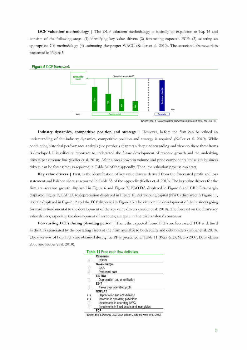
51

DCF valuation methodology | The DCF valuation methodology is basically an expansion of Eq. 16 and

consists of the following steps: (1) identifying key value drivers (2) forecasting expected FCFs (3) selecting an

appropriate CV methodology (4) estimating the proper WACC (Koller et al. 2010). The associated framework is

presented in Figure 5.

Figure 5 DCF framework

Source: Berk & DeMarzo (2007); Damodaran (2006) and Koller et al. (2010)

Industry dynamics, competitive position and strategy | However, before the firm can be valued an

understanding of the industry dynamics, competitive position and strategy is required (Koller et al. 2010). While

conducting historical performance analysis (see previous chapter) a deep understanding and view on these three items

is developed. It is critically important to understand the future development of revenue growth and the underlying

drivers per revenue line (Koller et al. 2010). After a breakdown in volume and price components, these key business

drivers can be forecasted, as reported in Table 34 of the appendix. Then, the valuation process can start.

Key value drivers | First, is the identification of key value drivers derived from the forecasted profit and loss

statement and balance sheet as reported in Table 35 of the appendix (Koller et al. 2010). The key value drivers for the

firm are: revenue growth displayed in Figure 6 and Figure 7, EBITDA displayed in Figure 8 and EBITDA-margin

displayed Figure 9, CAPEX to depreciation displayed in Figure 10, net working capital (NWC) displayed in Figure 11,

tax rate displayed in Figure 12 and the FCF displayed in Figure 13. The view on the development of the business going

forward is fundamental to the development of the key value drivers (Koller et al. 2010). The forecast on the firm’s key

value drivers, especially the development of revenues, are quite in line with analysts’ consensus.

Forecasting FCFs during planning period | Then, the expected future FCFs are forecasted. FCF is defined

as the CFs (generated by the operating assets of the firm) available to both equity and debt holders (Koller et al. 2010).

The overview of how FCFs are obtained during the PP is presented in Table 11 (Berk & DeMarzo 2007; Damodaran

2006 and Koller et al. 2010).

Table 11 Free cash flow definition Revenues (-) COGS Gross margin

(-) G&A (-) Personnel cost EBITDA

(-) Depreciation and amortization EBIT

(-) Taxes over operating profit NOPLAT

(+) Depreciation and amortization (+) Increase in operating provisions (-) Investments in operating NWC (-) Investments in fixed assets and intangibles

FCF Source: Berk & DeMarzo (2007); Damodaran (2006) and Koller et al. (2010)

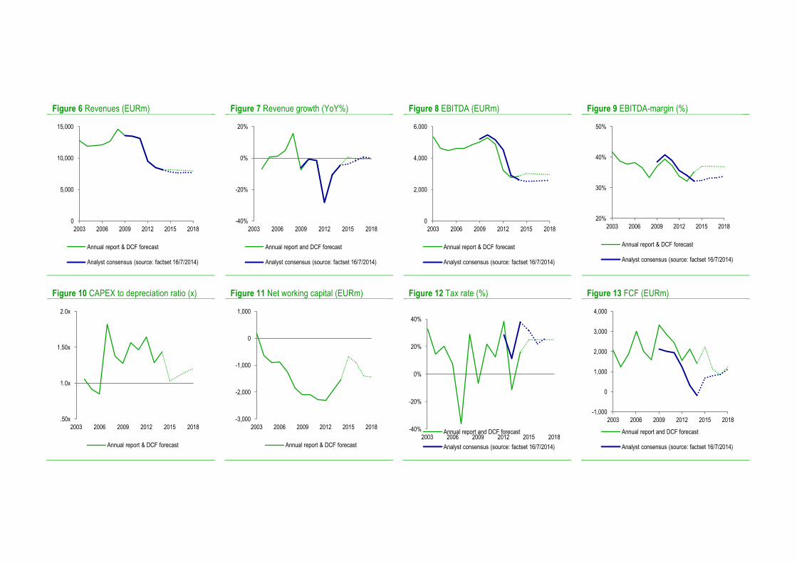
Figure 6 Revenues (EURm) Figure 7 Revenue growth (YoY%) Figure 8 EBITDA (EURm) Figure 9 EBITDA-margin (%)

Figure 10 CAPEX to depreciation ratio (x) Figure 11 Net working capital (EURm) Figure 12 Tax rate (%) Figure 13 FCF (EURm)

0

5,000

10,000

15,000

2003 2006 2009 2012 2015 2018

Annual report & DCF forecast

Analyst consensus (source: factset 16/7/2014)

-40%

-20%

0%

20%

2003 2006 2009 2012 2015 2018

Annual report and DCF forecast


0

2,000

4,000

6,000

2003 2006 2009 2012 2015 2018



20%

30%

40%

50%

2003 2006 2009 2012 2015 2018



.50x

1.0x

1.50x

2.0x

2003 2006 2009 2012 2015 2018


-3,000

-2,000

-1,000

0

1,000

2003 2006 2009 2012 2015 2018


-40%

-20%

0%

20%

40%

2003 2006 2009 2012 2015 2018Annual report and DCF forecast


-1,000

0

1,000

2,000

3,000

4,000

2003 2006 2009 2012 2015 2018

Annual report and DCF forecast


These CFs are obtained assuming the firm is all equity financed; the financing effects will be incorporated in the

valuation through the WACC (Koller et al. 2010).

Continuing value | Next, is the CV29 to be derived, which is the value of the business going forward, after the

PP (Koller et al. 2010). The value during and after the PP added together results in the EV (Koller et al. 2010). The

value-driver model for deriving the CV by Koller et al. (2010) assumes that the firm generates a RONIC higher than

the WACC. This implies that the firm maintains a competitive advantage in the near future (Koller et al. 2010). An

alternative model for estimating the CV, the ‘aggressive growth formula,’ is expected to overestimate the CV, as it

assumes that the firm will generate a RONIC which is approaching infinity (Koller et al. 2010). In contrast, the

‘converge model’ is expected to underestimate the CV of the firm, as it assumes that the firm will generate a RONIC

equal to the WACC (Koller et al. 2010). So, the formula for deriving the !"#$% (Eq. 17), which equals the key value

driver formula (Eq. 1), is (Koller et al. 2010):

!"#$% ='()*+,#-. 1 −

1 2#3(4!#

/(8+!! − 1 2# )

1 + 8+!! (#;<.>) Eq. 17

Where '()*+,#$% (Eq. 18) is the after-tax operating profit for all investors, which on its turn is defined as

(Koller et al. 2010):

'()*+,#$% = 1?4,#$% − (@ABCDEF2DCGAH#$% Eq. 18

1 2# (Eq. 19) is the estimated growth rate after the planning period and is defined as (Koller et al. 2010):

1 2# = 3(4!# ∗ 33# Eq. 19

3(4!# (Eq. 20) is the return on invested capital and is defined as (Koller et al. 2010):

3(4!# =

'()*+,#(@ABCDEF2JC@EDCK#

Eq. 20

33# (Eq. 21) is the reinvestment ratio and is defined as (Koller et al. 2010):

33# =

'ADEFLAHDMAFD#'()*+,#

Eq. 21

'ADEFLAHDMAFD# (Eq. 22) is defined as (Koller et al. 2010):

'ADEFLAHDMAFD# = 4FLAHDMAFDEF'8!# + ,NDCK!C@AG# − OA@BAJECDENF# Eq. 22

Summing the value during and after the PP (CV), results in the EV (Eq. 23) (Koller et al. 2010):

1" = )" P!P + )"(!") Eq. 23

29 The estimation of this value is critical as it significantly affects firm value (>50% of value) (Koller et al. 2010).

54

Adjustments to get to value of common equity is needed, because the CF implications of these assets and liabilities

are not reflected in the expected FCF (Koller et al. 2010). The final step to be taken is to derive the equity value from

the EV, this results in the value available to shareholders. The adjustments to the EV (Eq. 24) are as follows (Koller

et al. 2010):

1QREDSLCKRA = 1" + '(+ − 'NFAQREDSJKCEMH Eq. 24

Where nonequity claims are: short-term debt, long-term debt, unfunded retirement liabilities, capitalized

operating leases, and outstanding employee options (Koller et al. 2010).

Estimating WACC | The final step in the DCF valuation process, is to estimate the WACC (Eq. 25) (Koller et

al. 2010). The WACC is the “composite forward looking after tax cost of capital of the firm and forms the discount

factor for discounting the future expected CFs and CV, accounting for future CF risk” (Koller et al. 2010), and is

defined as:

8+!! = TU

1

1 + O+ TV(1 − WX)

O

(O + 1) Eq. 25

Where 1 and O are the proportion of equity and debt used to fund the business, TU is the cost of equity, TV is

the pretax cost of debt and WX is the tax rate. The cost of equity (TU) is estimated via the CAPM (Eq. 26) (Fama 1965):

TU = 1 3Y = BZ + [U,Y ]3) + ^P)Y Eq. 26

Where 1 3Y is the expected return for security E , BZ the risk free rate, ]3) the market risk premium. The

systematic market risk of the firm E’s ([U,Y), reflects the correlation of returns with the returns of the market portfolio

(Koller et al. 2010). The CAPM (Fama 1965) does not take into account the size of the firm, that may come with

limited liquidity, higher default risk and limited trading volumes (Koller et al. 2010). In order not to underestimate the

cost of equity (TU) of small caps, a small firm premium (^P)Y) is added (Koller et al. 2010). The ^P) depends on the

firm’s market capitalization (Koller et al. 2010), and is set in this case to 3.6%. The BZ is set to 1.5%; it is assumed that

the very low current yield on a ten year German government bond (0.34% at 31/12/2014) will overestimate the CV

of the firm. The ]3) is given by an internal department of the firm and is set to 6%, which is in line with the market

risk premium for well-developed capital markets (Koller et al. 2010). The equity beta ([U,Y) is derived by the relevering

the unlevered beta using the Hamada (1972) (Eq. 27) formula:

[U,Y = [_ 1 + 1 − WX

O

1 Eq. 27

Where [_ is the unlevered beta, implying that the firm is all equity financed (Hamada 1972), and reflects the risk

of the operating assets (Koller et al. 2010). The unlevered beta for the firm equals 0.5430. Further, WX is the tax rate and

O/1 the target ratio debt to equity. The cost of debt (TV) (Eq. 28) is estimated through the CAPM (Fama 1965) as

well, denoted as:

30 Source: Thomson Banker One (31/12/2014).

55

TV = BZ + [V ∗ ]3) + O3) Eq. 28

Where [V is the beta of debt and O3) is the default risk premium (3.5%). The cost of debt (TV) equals the

promised yield to maturity (Koller et al. 2010). This is given the duration and rating set to investment grade bond

(rating >BBB) (Koller et al. 2010). This is similar for high yield bonds (rating <BBB), with the exception that the

default probability is taken into account (Koller et al. 2010). This is approximated by the yield on a BBB bond

(Copeland 1979). The rating of Firm X is BBB-, which implies medium risk, resulting in a post-tax cost of debt (TV)

of 3.8% at a marginal tax rate of 25%.

Forecasting CE | Finally, the forecast on CE is estimated based on the CFOs resulting from the EBITDA

forecast. These values are inserted into the CE formula (Eq. 29) in combination with assumptions on the forward

looking retention rate (B#%àb), discount rate (c#%àb) and growth rate (2#%àb).

4.2 Customer-based valuation models

The forecast of individual customer behavior, hence individual customer CFs, is rather complex. The firm is

active in a multi-product industry, executing a multi-brand strategy, targeting multi-segments. This results in

multidimensional customer purchase behavior. Due to this complexity, two ‘basic’ methods are introduced first in

determining customer based benchmark values. First, a replication of the approach of Gupta et al. (2004) for calculating

historical CE from publicly available information. The historical development of CE is linked to the historical share

price of the firm, hence SHV. Then, in line with Donkers et al. (2003) a status quo model is developed. This model

assumes a constant forecast on the total of individual customer EBITDA contributions during the PP. Finally, based

on a combination of methods presented by Bolton et al. (2000), Donkers et al. (2003), Malthouse & Blattberg (2005)

and Verhoef & Donkers (2001) an advanced forecast model is developed. This CBB valuation model combines various

profit regression models in forecasting a customer’s EBITDA contribution, hence SHV. Nine predictors of the profit

models are ‘updated’ through various behavior logit models, forecasting individual customer behavior. The core of the

CBB valuation model is the customer behavior value driver spectrum as presented in Figure 2.

4.2.1 Customer equity valuation model

The method used for modelling historical CE based on publicly available data is to a large extent in accordance

with Gupta & Lehmann (2003) and Gupta et al. (2004) method. With the only remark that, in order to obtain more

accurate results, publicly available data is replaced by the firm’s internal data when available. The CE model used, relies

on the concept of CLV (Eq. 29), denoted as:

!1# = !*"Y,# = MY,#BY,#

1 + c# − BY,#∗ 1 + 2Y,# Eq. 29

Where !1# at time D is the sum of all individual customer E lifetime values, MY,# is the margin, BY,# the retention

rate, c# the discount rate and 2Y,# is the growth rate incorporating acquisition.

Model input | As a first input, the calculated annual CFOs (2003–2014) as displayed in Figure 14, serve as a

proxy for margin (MY,#).

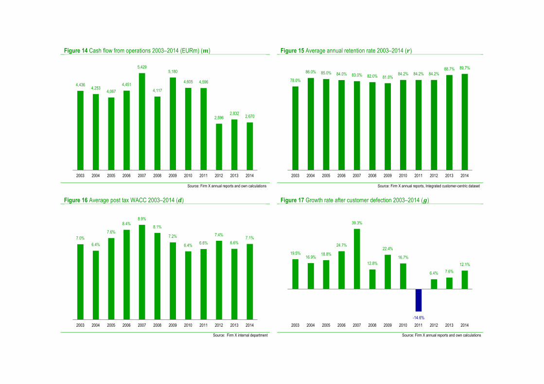
Figure 14 Cash flow from operations 2003–2014 (EURm) (!) Figure 15 Average annual retention rate 2003–2014 (")

Source: Firm X annual reports and own calculations Source: Firm X annual reports, Integrated customer-centric dataset

Figure 16 Average post tax WACC 2003–2014 (#) Figure 17 Growth rate after customer defection 2003–2014 ($)

Source: Firm X internal department Source: Firm X annual reports and own calculations

4,4364,253

4,0674,451

5,429

4,117

5,180

4,605 4,596

2,5962,832

2,670

2003 2004 2005 2006 2007 2008 2009 2010 2011 2012 2013 2014

78.0%

86.0% 85.0% 84.0% 83.0% 82.0% 81.0%84.2% 84.2% 84.2%

88.7% 89.7%

2003 2004 2005 2006 2007 2008 2009 2010 2011 2012 2013 2014

7.0%6.4%

7.6%

8.4%8.9%

8.1%

7.2%

6.4% 6.6%

7.4%

6.6%7.1%

2003 2004 2005 2006 2007 2008 2009 2010 2011 2012 2013 2014

19.5%16.9%

18.8%

24.7%

39.3%

12.8%

22.4%

16.7%

-14.6%

6.4% 7.6%12.1%

2003 2004 2005 2006 2007 2008 2009 2010 2011 2012 2013 2014

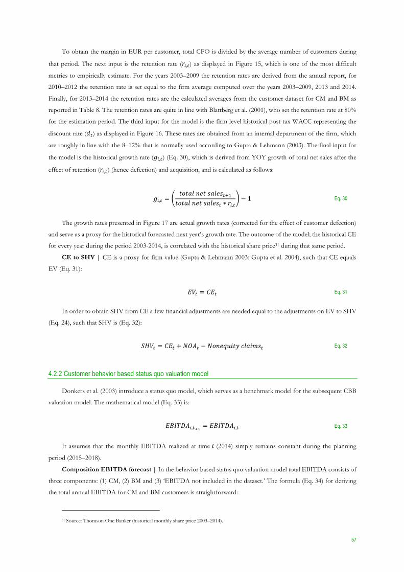
57

To obtain the margin in EUR per customer, total CFO is divided by the average number of customers during

that period. The next input is the retention rate (!",$) as displayed in Figure 15, which is one of the most difficult

metrics to empirically estimate. For the years 2003–2009 the retention rates are derived from the annual report, for

2010–2012 the retention rate is set equal to the firm average computed over the years 2003–2009, 2013 and 2014.

Finally, for 2013–2014 the retention rates are the calculated averages from the customer dataset for CM and BM as

reported in Table 8. The retention rates are quite in line with Blattberg et al. (2001), who set the retention rate at 80%

for the estimation period. The third input for the model is the firm level historical post-tax WACC representing the

discount rate (%$) as displayed in Figure 16. These rates are obtained from an internal department of the firm, which

are roughly in line with the 8–12% that is normally used according to Gupta & Lehmann (2003). The final input for

the model is the historical growth rate (&",$) (Eq. 30), which is derived from YOY growth of total net sales after the

effect of retention (!",$) (hence defection) and acquisition, and is calculated as follows:

&",$ =

()(*+-.(/*+./$01()(*+-.(/*+./$ ∗ !",$

− 1 Eq. 30

The growth rates presented in Figure 17 are actual growth rates (corrected for the effect of customer defection)

and serve as a proxy for the historical forecasted next year’s growth rate. The outcome of the model; the historical CE

for every year during the period 2003-2014, is correlated with the historical share price31 during that same period.

CE to SHV | CE is a proxy for firm value (Gupta & Lehmann 2003; Gupta et al. 2004), such that CE equals

EV (Eq. 31):

56$ = 75$ Eq. 31

In order to obtain SHV from CE a few financial adjustments are needed equal to the adjustments on EV to SHV

(Eq. 24), such that SHV is (Eq. 32):

896$ = 75$ + ;<=$ − ;)-.>?@(AB+*@C/$ Eq. 32

4.2.2 Customer behavior based status quo valuation model

Donkers et al. (2003) introduce a status quo model, which serves as a benchmark model for the subsequent CBB

valuation model. The mathematical model (Eq. 33) is:

5DEFG=",$HI = 5DEFG=",$ Eq. 33

It assumes that the monthly EBITDA realized at time ( (2014) simply remains constant during the planning

period (2015–2018).

Composition EBITDA forecast | In the behavior based status quo valuation model total EBITDA consists of

three components: (1) CM, (2) BM and (3) ‘EBITDA not included in the dataset.’ The formula (Eq. 34) for deriving

the total annual EBITDA for CM and BM customers is straightforward:

31 Source: Thomson One Banker (historical monthly share price 2003–2014).

58

J",$ = <K-"L,$ ∗ M.N"L,$ ∗ 5DEFG=OL,$ ∗ 12"

Eq. 34

Where J",$ is the sum of EBITDA contribution per individual customer @, <K-"L,$ is a dummy for ownership for

a particular BSP-combination (Q) at time (, M.N"L,$ and 5DEFG=OL,$ are the corresponding revenues and EBITDA-

margins aggregated on the BSP-level Q, as reported in Table 5. The EBITDA that is not included in the dataset

(5DEFG=RSRTU,$), as a consequence of data availability (see chapter 3), is an average-based estimate (2013–2014;

(V1, (). The estimated amount is added as a fixed amount to every single year of the forecast and is calculated as follows

(Eq. 35 through Eq. 37):

5DEFG=RSRTU,$ = 5DEFG=WXW,$ − 5(5DEFG=SRTU,$) Eq. 35

Where, 5DEFG=WXW,$ is total EBITDA reported in the annual report, 5(5DEFG=SRTU,$) is the ‘normally’

expected amount of EBITDA included in the dataset as a percentage of included revenues in the dataset, at time (.

Then, 5(5DEFG=SRTU,$) (Eq. 36) is calculated as follows:

5(5DEFG=SRTU,$) = 5DEFG=OWXW,$ ∗ M.NSRTU,",$ Eq. 36

Where 5DEFG=OWXW,$ is the total EBITDA-margin and M.NSRTU,",$ is the sum of the revenues for all

individual customer @’s included in the dataset, at time (. The total EBITDA-margin (5DEFG=OWXW,$) (Eq. 37) is

calculated as follows:

5DEFG=OWXW,$ =

5DEFG=WXW,$M.NWXW,$

Eq. 37

Where, 5DEFG=WXW,$ is the total EBITDA and M.NWXW,$ are total revenues at time (, taken from the annual

report of the firm.

Merging forecast output | In order to obtain the amount of SHV from the customer behavior based status

quo valuation model forecast, the obtained EBITDA during the planning period is inserted into the DCF valuation

model. Both models merge on the level of ‘EBITDA’ as presented in Table 11. From here the last part of the model

continues until the end with DCF valuation methodology.

4.2.3 Customer behavior based valuation model

The CBB valuation model originates from a combination of methods presented by Bolton et al. (2000), Donkers

et al. (2003), Malthouse & Blattberg (2005) and Verhoef & Donkers (2001). The derived framework is displayed in

Figure 18, revealing that the model forecast is entirely algorithm driven. For each year of the PP (2015–2018) 4

horizontal ‘main-algorithms,’ forecast an individual customer’s EBITDA contribution. Then, 9 vertical sub-algorithms

‘update’ the predictor values, the customer behavior value driver probability, based on Figure 2, in each of the 4 ‘main-

algorithms.’ The ‘main-algorithms’ consists of a multiple linear regression model, called the ‘profit regression models.’

And the ‘sub-algorithms’ consists of a binary logistic regression model, called the ‘behavior logit models.’

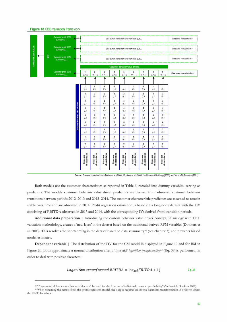
59

Figure 18 CBB valuation framework

Source: Framework derived from Bolton et al. (2000), Donkers et al. (2003), Malthouse & Blattberg (2005) and Verhoef & Donkers (2001)

Both models use the customer characteristics as reported in Table 6, recoded into dummy variables, serving as

predictors. The models customer behavior value driver predictors are derived from observed customer behavior

transitions between periods 2012–2013 and 2013–2014. The customer characteristic predictors are assumed to remain

stable over time and are observed in 2014. Profit regression estimation is based on a long-body dataset with the DV

consisting of EBITDA observed in 2013 and 2014, with the corresponding IVs derived from transition periods.

Additional data preparation | Introducing the custom behavior value driver concept, in analogy with DCF

valuation methodology, creates a ‘new layer’ in the dataset based on the traditional derived RFM variables (Donkers et

al. 2003). This resolves the shortcoming in the dataset based on data asymmetry32 (see chapter 3), and prevents biased

model estimates.

Dependent variable | The distribution of the DV for the CM model is displayed in Figure 19 and for BM in

Figure 20. Both approximate a normal distribution after a ‘first-aid’ logarithm transformation33 (Eq. 38) is performed, in

order to deal with positive skewness:

[)&*!@(ℎC(!*-/])!C.%5DEFG= = log1a(5DEFG= + 1) Eq. 38

32 “Asymmetrical data causes that variables can’t be used for the forecast of individual customer profitability” (Verhoef & Donkers 2001). 33 When obtaining the results from the profit regression model, the output requires an inverse logarithm transformation in order to obtain

the EBITDA values.

DCF

Customer profit 2018!"#$%&'( ,*+4

Customer profit 2017!"#$%&'(,*+ -

Customer profit 2016!"#$%&'(,*+ .

Customer profit 2015!"#$%&'(,*+ /

101,*23 Customer characteristics

101,*

201,*23

301,*23

401,*23

501,*23

601,*23

701,*23

201,*

801,*23

901,*23

301,*401,*501,*601,*701,*801,*901,*

101,*

201,*301,*401,*501,*601,*701,*801,*901,*

Cust

omer

ch

arac

teris

tics

Cust

omer

ch

arac

teris

tics

101,*201,*301,*401,*501,*601,*701,*801,*901,*

101,*201,*301,*401,*501,*601,*701,*801,*901,*

Cust

omer

ch

arac

teris

tics

Cust

omer

ch

arac

teris

tics

101,*201,*301,*401,*501,*601,*701,*801,*901,*

101,*201,*301,*401,*501,*601,*701,*801,*901,*

Cust

omer

ch

arac

teris

tics

Cust

omer

ch

arac

teris

tics

101,*201,*301,*401,*501,*601,*701,*801,*901,*

101,*201,*301,*401,*501,*601,*701,*801,*901,*

Cust

omer

ch

arac

teris

tics

Cust

omer

ch

arac

teris

tics

Customer behavior value drivers

Cust

omer

ch

arac

teris

tics

Cust

omer

beh

avio

r val

ue d

river

s

101,*201,*301,*401,*501,*601,*701,*801,*901,*

Customerbehaviorvaluedrivers01, *24






SHAR

EHOL

DER

VALU

E

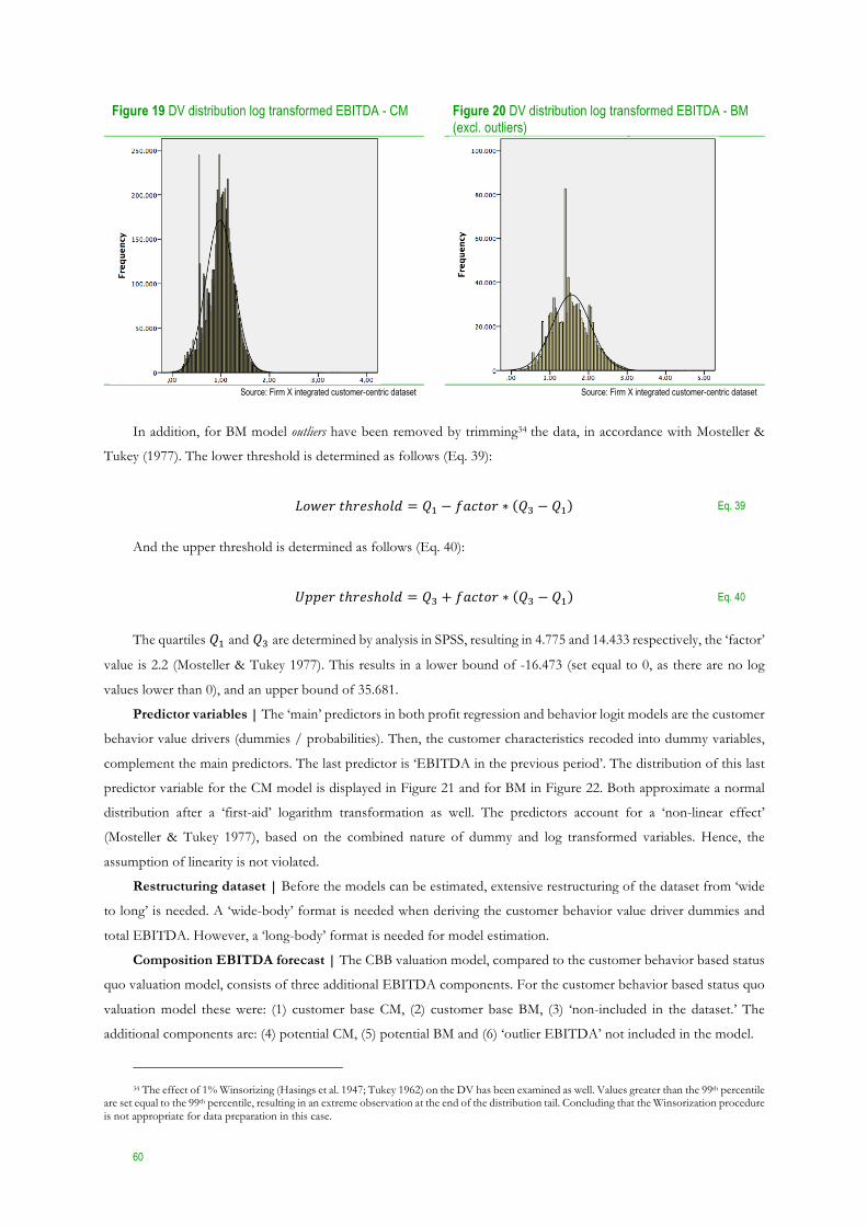
60

Figure 19 DV distribution log transformed EBITDA - CM Figure 20 DV distribution log transformed EBITDA - BM (excl. outliers)

Source: Firm X integrated customer-centric dataset Source: Firm X integrated customer-centric dataset

In addition, for BM model outliers have been removed by trimming34 the data, in accordance with Mosteller &

Tukey (1977). The lower threshold is determined as follows (Eq. 39):

[)K.!(ℎ!./ℎ)+% = b1 − ]*B()! ∗ bc − b1 Eq. 39

And the upper threshold is determined as follows (Eq. 40):

dee.!(ℎ!./ℎ)+% = bc + ]*B()! ∗ bc − b1 Eq. 40

The quartiles b1 and bc are determined by analysis in SPSS, resulting in 4.775 and 14.433 respectively, the ‘factor’

value is 2.2 (Mosteller & Tukey 1977). This results in a lower bound of -16.473 (set equal to 0, as there are no log

values lower than 0), and an upper bound of 35.681.

Predictor variables | The ‘main’ predictors in both profit regression and behavior logit models are the customer

behavior value drivers (dummies / probabilities). Then, the customer characteristics recoded into dummy variables,

complement the main predictors. The last predictor is ‘EBITDA in the previous period’. The distribution of this last

predictor variable for the CM model is displayed in Figure 21 and for BM in Figure 22. Both approximate a normal

distribution after a ‘first-aid’ logarithm transformation as well. The predictors account for a ‘non-linear effect’

(Mosteller & Tukey 1977), based on the combined nature of dummy and log transformed variables. Hence, the

assumption of linearity is not violated.

Restructuring dataset | Before the models can be estimated, extensive restructuring of the dataset from ‘wide

to long’ is needed. A ‘wide-body’ format is needed when deriving the customer behavior value driver dummies and

total EBITDA. However, a ‘long-body’ format is needed for model estimation.

Composition EBITDA forecast | The CBB valuation model, compared to the customer behavior based status

quo valuation model, consists of three additional EBITDA components. For the customer behavior based status quo

valuation model these were: (1) customer base CM, (2) customer base BM, (3) ‘non-included in the dataset.’ The

additional components are: (4) potential CM, (5) potential BM and (6) ‘outlier EBITDA’ not included in the model.

34 The effect of 1% Winsorizing (Hasings et al. 1947; Tukey 1962) on the DV has been examined as well. Values greater than the 99th percentile

are set equal to the 99th percentile, resulting in an extreme observation at the end of the distribution tail. Concluding that the Winsorization procedure is not appropriate for data preparation in this case.

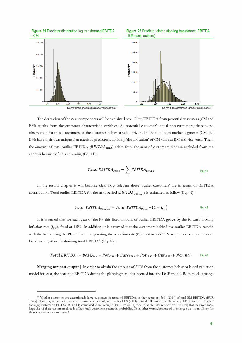
61

Figure 21 Predictor distribution log transformed EBITDA - CM

Figure 22 Predictor distribution log transformed EBITDA - BM (excl. outliers)

Source: Firm X integrated customer-centric dataset Source: Firm X integrated customer-centric dataset

The derivation of the new components will be explained next. First, EBITDA from potential customers (CM and

BM) results from the customer characteristic variables. As potential customer’s equal non-customers, there is no

observation for these customers on the customer behavior value drivers. In addition, both market segments (CM and

BM) have their own unique characteristic predictors, avoiding ‘the allocation’ of CM value at BM and vice versa. Then,

the amount of total outlier EBITDA (5DEFG=fg$,$) arises from the sum of customers that are excluded from the

analysis because of data trimming (Eq. 41):

F)(*+5DEFG=fg$,$ = 5DEFG=",fg$,$"

Eq. 41

In the results chapter it will become clear how relevant these ‘outlier-customers’ are in terms of EBITDA

contribution. Total outlier EBITDA for the next period (5DEFG=fg$,$HI) is estimated as follow (Eq. 42):

F)(*+5DEFG=fg$,$HI = F)(*+5DEFG=fg$,$ ∗ 1 + @h,$ Eq. 42

It is assumed that for each year of the PP this fixed amount of outlier EBITDA grows by the forward looking

inflation rate (@h,$), fixed at 1.5%. In addition, it is assumed that the customers behind the outlier EBITDA remain

with the firm during the PP, so that incorporating the retention rate (!) is not needed35. Now, the six components can

be added together for deriving total EBITDA (Eq. 43):

F)(*+5DEFG=$ = D*/.Ti,$ + j)(.Ti,$+ D*/.li,$ + j)(.li,$+ <?(.li,$+ ;)-@-B+$ Eq. 43

Merging forecast output | In order to obtain the amount of SHV from the customer behavior based valuation

model forecast, the obtained EBITDA during the planning period is inserted into the DCF-model. Both models merge

35 "Outlier customers are exceptionally large customers in terms of EBITDA, as they represent 56% (2014) of total BM EBITDA (EUR

764m). However, in terms of numbers of customers they only account for 1.8% (2014) of total BM customers. The average EBITDA for an ‘outlier’ (or large) customer is EUR 65,000 (2014), compared to an average of EUR 955 (2014) for all other business customers. It is likely that the exceptional large size of these customers directly affects each customer’s retention probability. Or in other words, because of their large size it is not likely for these customers to leave Firm X.

62

on the level of ‘EBITDA’ as presented in Table 11. From here the last part of the model continues with DCF valuation

methodology.

SHV range (95% CI) | EBITDA is calculated for three different scenarios: the base case, low and high. For the

low- and high-scenarios, parameter estimates for the lower and upper bound of the 95% CI are used. Then, for each

scenario the 4 profit equations and 9 behavior logit36 equations are solved, resulting in three EBITDA values per

customer. These values then again merge into the DCF valuation model. The behavior logit models report exponential

betas on the CI estimates. In order to prepare these parameters for equation solving, the inverse needs to be obtained

(Eq. 44):

m = ln .o Eq. 44

SHV contribution per customer behavior value driver | Next, now that scenario analysis has set the lower

and upper bound of the SHV range, is to determine the SHV contribution range per customer behavior value driver.

In order to obtain the range of SHV contribution per driver, the value is estimated for the low and high scenarios. The

exact same procedure for estimating the SHV range is applied here as well. However, there is one difference. In order

to estimate the isolated SHV contribution of one customer behavior value driver, the SHV is estimated by eliminating37

the concerning driver. In other words, all corresponding values are set to ‘0’ for the concerning value driver. Now

SHV can be estimated without the concerning customer behavior value driver. Then, this SHV outcome is subtracted

from the ‘full-model’ (including all value drivers) outcome, resulting in the SHV contribution for the corresponding

customer behavior value driver.

Incremental SHV at customer behavior value driver improvement | Almost a similar method will be applied

in determining the impact of an improvement of a particular customer behavior value driver. However, an

improvement in value driver means in practice an improvement of the customer probability for the corresponding

value driver. This implies that for all customers in the customer base their probability on a value driver is improved by

a certain fixed percentage. Then again, the difference in outcome is the estimated incremental SHV when improving

the customer probabilities for the concerning value driver.

Forecasting CE | Finally, the forecast on CE is estimated based on the CFOs resulting from the EBITDA

forecast. These values are inserted into the CE formula (Eq. 29) in combination with assumptions on the forward

looking retention rate (!$Ipqr), discount rate (%$Ipqr) and growth rate (&$Ipqr).

4.2.3.1 Profit regression model

The profit regression model is a multiple linear regression model, aiming to forecast a customer’s EBITDA

contribution (Malthouse & Blattberg 2005) for each year of the planning period (2015–2018). The general idea behind

the profit regression model is as follows (Eq. 45):

5DEFG="L,$HI"

= ] j st"L,$HI , 5t"L,$, 7t"L Eq. 45

36 For the logit equations, for each year the same scenario-type output is used as input for the same scenario-type in the next year. Or in other

words, the output for the low-scenario is used as input for the low-scenario of the next period. 37 Given that all else remains the same.

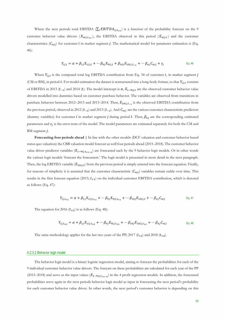
63

Where the next periods total EBITDA ( 5DEFG="L,$HI" ) is a function of the probability forecast on the 9

customer behavior value drivers (st"L,$HI ), the EBITDA observed in this period (5t"L,$ ) and the customer

characteristics (7t"L) for customer @ in market segment Q. The mathematical model for parameter estimation is (Eq.

46):

J"L,$ = u + m1Ls1"L,$ + ⋯mwLsw"L,$ + m1aL51a"L,$xI + ⋯mtL7t"L + yL Eq. 46

Where J"L,$ is the computed total log EBITDA contribution from Eq. 34 of customer @, in market segment Q

(CM or BM), in period (. For model estimation the dataset is restructured into a long-body format, so that J"L,$ consists

of EBITDA in 2013 ((V1) and 2014 ((). The model intercept is u, s1Vw"L,$ are the observed customer behavior value

drivers modelled into dummies based on customer purchase behavior. The variables are observed from transitions in

purchase behavior between 2012–2013 and 2013–2014. Then, 51a"L,$xI is the observed EBITDA contribution from

the previous period, observed in 2012 ((Vz) and 2013 ((V1). And 7t"L are the various customer characteristic predictors

(dummy variables) for customer @ in market segment Q during period (. Then, mtL are the corresponding estimated

parameters and yL is the error term of the model. The model parameters are estimated separately for both the CM and

BM segment Q.

Forecasting four periods ahead | In line with the other models (DCF valuation and customer behavior based

status quo valuation) the CBB valuation model forecast as well four periods ahead (2015–2018). The customer behavior

value driver predictor variables (s1Vw"L,$HIxr) are forecasted each by the 9 behavior logit models. Or in other words

the various logit models ‘forecast the forecasters.’ The logit model is presented in more detail in the next paragraph.

Then, the log EBITDA variable (51a"L,$) from the previous period is simply entered into the forecast equation. Finally,

for reasons of simplicity it is assumed that the customer characteristic (7t"L) variables remain stable over time. This

results in the first forecast equation (2015; (01) on the individual customer EBITDA contribution, which is denoted

as follows (Eq. 47):

J"L,$HI = u + m1Ls1"L,$HI + ⋯mwLsw"L,$HI + ⋯m1aL51a"L,$ + ⋯mtL7t"L Eq. 47

The equation for 2016 ((0z) is as follows (Eq. 48):

J"L,$H{ = u + m1Ls1"L,$H{ + ⋯mwLsw"L,$H{ + ⋯m1aL51a"L,$HI + ⋯mtL7t"L Eq. 48

The same methodology applies for the last two years of the PP; 2017 ((0c) and 2018 ((0|).

4.2.3.2 Behavior logit model

The behavior logit model is a binary logistic regression model, aiming to forecast the probabilities for each of the

9 individual customer behavior value drivers. The forecast on these probabilities are calculated for each year of the PP

(2015–2018) and serve as the input values (s1Vw"L,$HIxr) in the 4 profit regression models. In addition, the forecasted

probabilities serve again in the next periods behavior logit model as input in forecasting the next period’s probability

for each customer behavior value driver. In other words, the next period’s customer behavior is depending on this

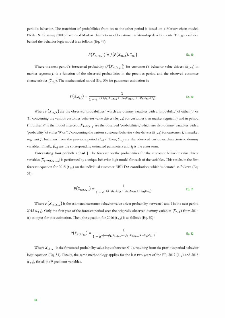
64

period’s behavior. The transition of probabilities from on to the other period is based on a Markov chain model.

Pfeifer & Carraway (2000) have used Markov chains to model customer relationship developments. The general idea

behind the behavior logit model is as follows (Eq. 49):

j st"L,$HI = ] j st"L,$ , 7t"L Eq. 49

Where the next period’s forecasted probability (j st"L,$HI ) for customer @’s behavior value drivers (-1Vw) in

market segment Q, is a function of the observed probabilities in the previous period and the observed customer

characteristics (7t"L). The mathematical model (Eq. 50) for parameter estimation is:

j st"L,$ =

11 + .V(}0oI~�IÄ,pxI0⋯oÅ~�ÅÄ~,pxI0⋯oÇ~TÇÄ~0É~)

Eq. 50

Where j st"L,$ are the observed ‘probabilities,’ which are dummy variables with a ‘probability’ of either ‘0’ or

‘1,’ concerning the various customer behavior value drivers (-1Vw) for customer @, in market segment Q and in period

(. Further, u is the model intercept, s1Vw",$xI are the observed ‘probabilities,’ which are also dummy variables with a

‘probability’ of either ‘0’ or ‘1,’ concerning the various customer behavior value drivers (-1Vw) for customer @, in market

segment Q, but then from the previous period ((V1). Then, 7t"L are the observed customer characteristic dummy

variables. Finally, mtL are the corresponding estimated parameters and yL is the error term.

Forecasting four periods ahead | The forecast on the probabilities for the customer behavior value driver

variables (s1Vw"L,$HIxr) is performed by a unique behavior logit model for each of the variables. This results in the first

forecast equation for 2015 ((01) on the individual customer EBITDA contribution, which is denoted as follows (Eq.

51):

j st"L,$HI =

1

1 + .V }0oI~�IÄ,p0⋯oÅ~�ÅÄ~,p0⋯oÇ~TÇÄ~ Eq. 51

Where j st"L,$HI is the estimated customer behavior value driver probability between 0 and 1 in the next period

2015 ((01). Only the first year of the forecast period uses the originally observed dummy variables (st",$) from 2014

(() as input for this estimation. Then, the equation for 2016 ((0z) is as follows (Eq. 52):

j st"L,$H{ =

1

1 + .V }0oI~�IÄ,pHI0⋯oÅ~�ÅÄ~,pHI0⋯oÇ~TÇÄ~ Eq. 52

Where s1",$HI is the forecasted probability value input (between 0–1), resulting from the previous period behavior

logit equation (Eq. 51). Finally, the same methodology applies for the last two years of the PP, 2017 ((0c) and 2018

((0|), for all the 9 predictor variables.

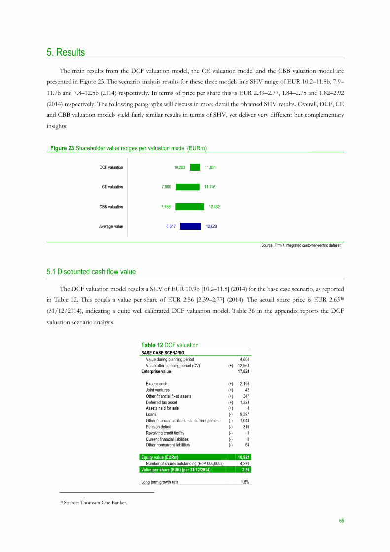
65

5. Results The main results from the DCF valuation model, the CE valuation model and the CBB valuation model are

presented in Figure 23. The scenario analysis results for these three models in a SHV range of EUR 10.2–11.8b, 7.9–

11.7b and 7.8–12.5b (2014) respectively. In terms of price per share this is EUR 2.39–2.77, 1.84–2.75 and 1.82–2.92

(2014) respectively. The following paragraphs will discuss in more detail the obtained SHV results. Overall, DCF, CE

and CBB valuation models yield fairly similar results in terms of SHV, yet deliver very different but complementary

insights.

Figure 23 Shareholder value ranges per valuation model (EURm)

Source: Firm X integrated customer-centric dataset

5.1 Discounted cash flow value

The DCF valuation model results a SHV of EUR 10.9b [10.2–11.8] (2014) for the base case scenario, as reported

in Table 12. This equals a value per share of EUR 2.56 [2.39–2.77] (2014). The actual share price is EUR 2.6338

(31/12/2014), indicating a quite well calibrated DCF valuation model. Table 36 in the appendix reports the DCF

valuation scenario analysis.

Table 12 DCF valuation BASE CASE SCENARIO

Value during planning period 4,860 Value after planning period (CV) (+) 12,968

Enterprise value 17,828

Excess cash (+) 2,195 Joint ventures (+) 42 Other financial fixed assets (+) 347 Deferred tax asset (+) 1,323 Assets held for sale (+) 8 Loans (-) 9,397 Other financial liabilities incl. current portion (-) 1,044 Pension deficit (-) 316 Revolving credit facility (-) 0 Current financial liabilities (-) 0 Other noncurrent liabilities (-) 64

Equity value (EURm) 10,922

Number of shares outstanding (EoP 000,000s) 4,270 Value per share (EUR) (per 31/12/2014) 2.56 Long term growth rate 1.5%

38 Source: Thomson One Banker.

10,203

7,860

7,788

8,617

11,831

11,746

12,482

12,020

DCF valuation

CE valuation

CBB valuation

Average value

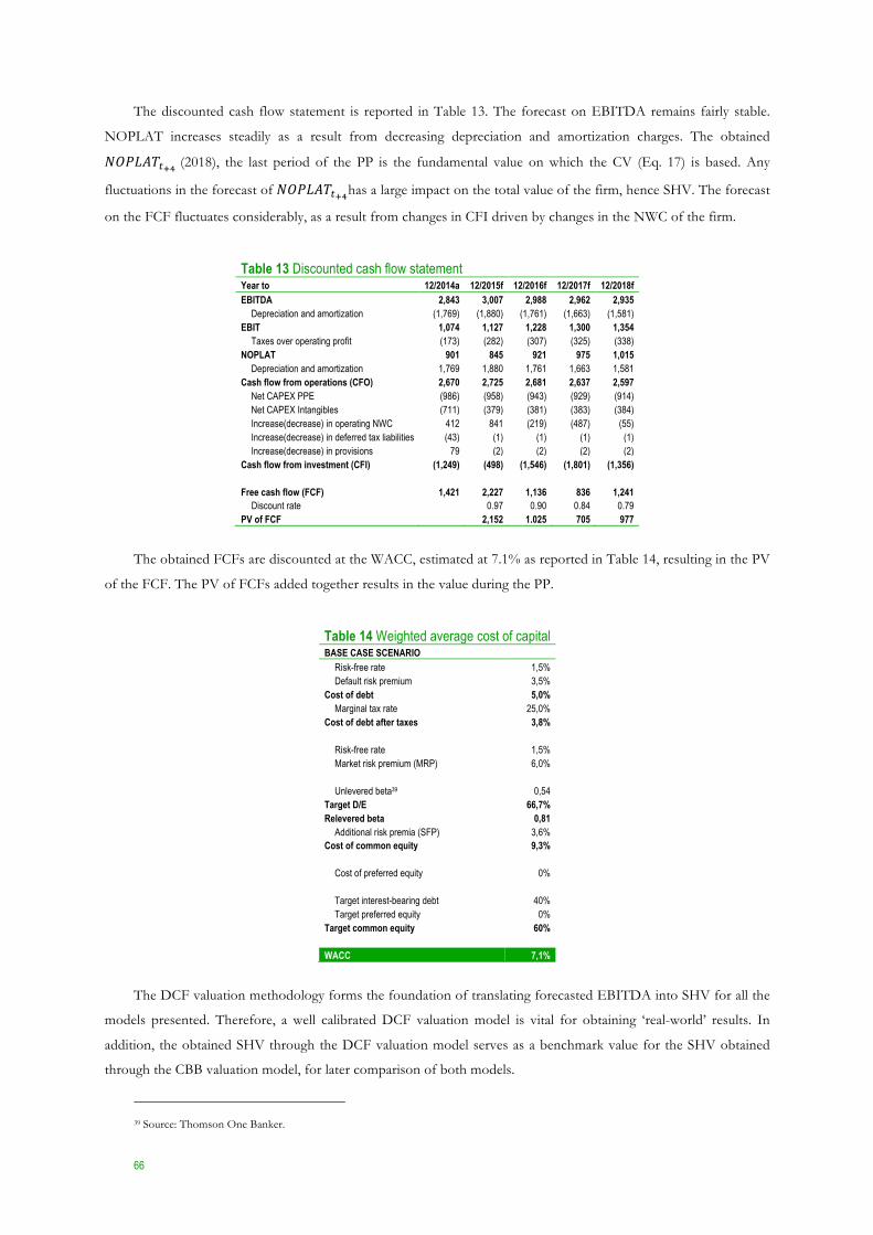
66

The discounted cash flow statement is reported in Table 13. The forecast on EBITDA remains fairly stable.

NOPLAT increases steadily as a result from decreasing depreciation and amortization charges. The obtained

;<j[=F$Hr (2018), the last period of the PP is the fundamental value on which the CV (Eq. 17) is based. Any

fluctuations in the forecast of ;<j[=F$Hrhas a large impact on the total value of the firm, hence SHV. The forecast

on the FCF fluctuates considerably, as a result from changes in CFI driven by changes in the NWC of the firm.

Table 13 Discounted cash flow statement Year to 12/2014a 12/2015f 12/2016f 12/2017f 12/2018f EBITDA 2,843 3,007 2,988 2,962 2,935

Depreciation and amortization (1,769) (1,880) (1,761) (1,663) (1,581) EBIT 1,074 1,127 1,228 1,300 1,354

Taxes over operating profit (173) (282) (307) (325) (338) NOPLAT 901 845 921 975 1,015

Depreciation and amortization 1,769 1,880 1,761 1,663 1,581 Cash flow from operations (CFO) 2,670 2,725 2,681 2,637 2,597

Net CAPEX PPE (986) (958) (943) (929) (914) Net CAPEX Intangibles (711) (379) (381) (383) (384) Increase(decrease) in operating NWC 412 841 (219) (487) (55) Increase(decrease) in deferred tax liabilities (43) (1) (1) (1) (1) Increase(decrease) in provisions 79 (2) (2) (2) (2)

Cash flow from investment (CFI) (1,249) (498) (1,546) (1,801) (1,356)

Free cash flow (FCF) 1,421 2,227 1,136 836 1,241 Discount rate 0.97 0.90 0.84 0.79

PV of FCF 2,152 1.025 705 977

The obtained FCFs are discounted at the WACC, estimated at 7.1% as reported in Table 14, resulting in the PV

of the FCF. The PV of FCFs added together results in the value during the PP.

Table 14 Weighted average cost of capital BASE CASE SCENARIO

Risk-free rate 1,5% Default risk premium 3,5%

Cost of debt 5,0% Marginal tax rate 25,0%

Cost of debt after taxes 3,8%

Risk-free rate 1,5% Market risk premium (MRP) 6,0%

Unlevered beta39 0,54

Target D/E 66,7% Relevered beta 0,81

Additional risk premia (SFP) 3,6% Cost of common equity 9,3%

Cost of preferred equity 0%

Target interest-bearing debt 40% Target preferred equity 0%

Target common equity 60%

WACC 7,1%

The DCF valuation methodology forms the foundation of translating forecasted EBITDA into SHV for all the

models presented. Therefore, a well calibrated DCF valuation model is vital for obtaining ‘real-world’ results. In

addition, the obtained SHV through the DCF valuation model serves as a benchmark value for the SHV obtained

through the CBB valuation model, for later comparison of both models.

39 Source: Thomson One Banker.

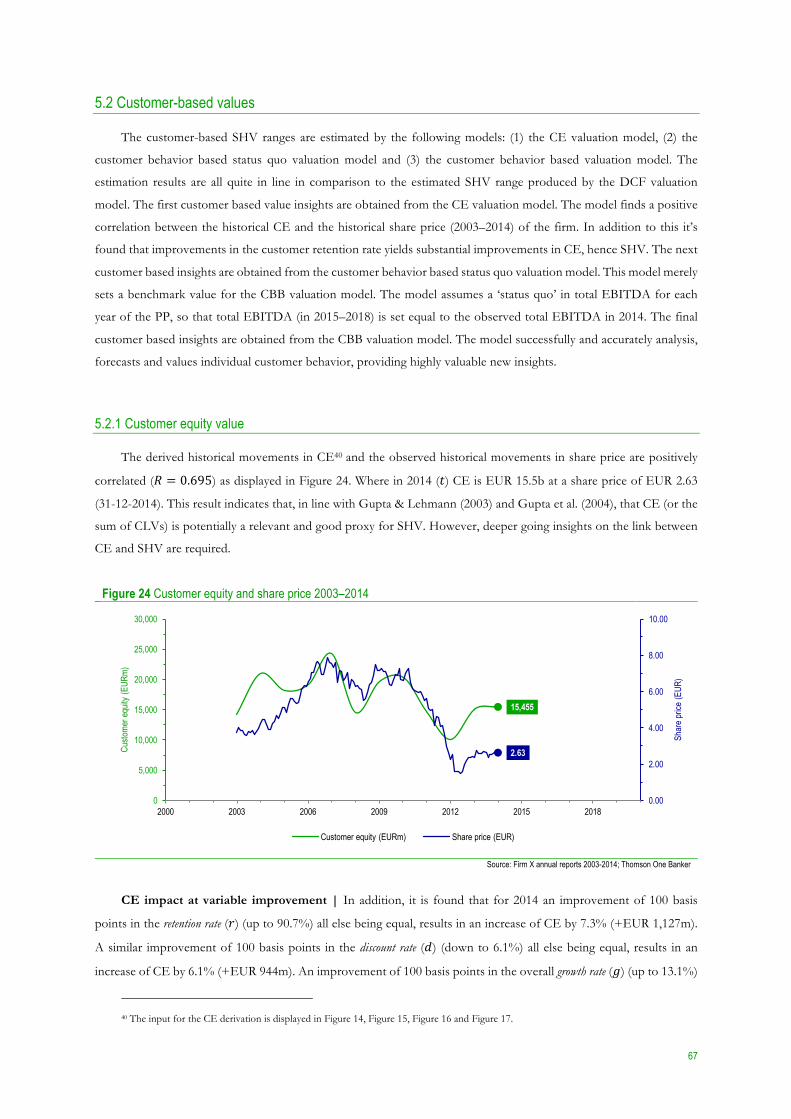
67

5.2 Customer-based values

The customer-based SHV ranges are estimated by the following models: (1) the CE valuation model, (2) the

customer behavior based status quo valuation model and (3) the customer behavior based valuation model. The

estimation results are all quite in line in comparison to the estimated SHV range produced by the DCF valuation

model. The first customer based value insights are obtained from the CE valuation model. The model finds a positive

correlation between the historical CE and the historical share price (2003–2014) of the firm. In addition to this it’s

found that improvements in the customer retention rate yields substantial improvements in CE, hence SHV. The next

customer based insights are obtained from the customer behavior based status quo valuation model. This model merely

sets a benchmark value for the CBB valuation model. The model assumes a ‘status quo’ in total EBITDA for each

year of the PP, so that total EBITDA (in 2015–2018) is set equal to the observed total EBITDA in 2014. The final

customer based insights are obtained from the CBB valuation model. The model successfully and accurately analysis,

forecasts and values individual customer behavior, providing highly valuable new insights.

5.2.1 Customer equity value

The derived historical movements in CE40 and the observed historical movements in share price are positively

correlated (M = 0.695) as displayed in Figure 24. Where in 2014 (() CE is EUR 15.5b at a share price of EUR 2.63

(31-12-2014). This result indicates that, in line with Gupta & Lehmann (2003) and Gupta et al. (2004), that CE (or the

sum of CLVs) is potentially a relevant and good proxy for SHV. However, deeper going insights on the link between

CE and SHV are required.

Figure 24 Customer equity and share price 2003–2014

Source: Firm X annual reports 2003-2014; Thomson One Banker

CE impact at variable improvement | In addition, it is found that for 2014 an improvement of 100 basis

points in the retention rate (!) (up to 90.7%) all else being equal, results in an increase of CE by 7.3% (+EUR 1,127m).

A similar improvement of 100 basis points in the discount rate (%) (down to 6.1%) all else being equal, results in an

increase of CE by 6.1% (+EUR 944m). An improvement of 100 basis points in the overall growth rate (&) (up to 13.1%)

40 The input for the CE derivation is displayed in Figure 14, Figure 15, Figure 16 and Figure 17.

15,455

2.63

0.00

2.00

4.00

6.00

8.00

10.00

0

5,000

10,000

15,000

20,000

25,000

30,000

2000 2003 2006 2009 2012 2015 2018

Shar

e pr

ice (E

UR)

Custo

mer

equ

ity (E

URm

)

Customer equity (EURm) Share price (EUR)

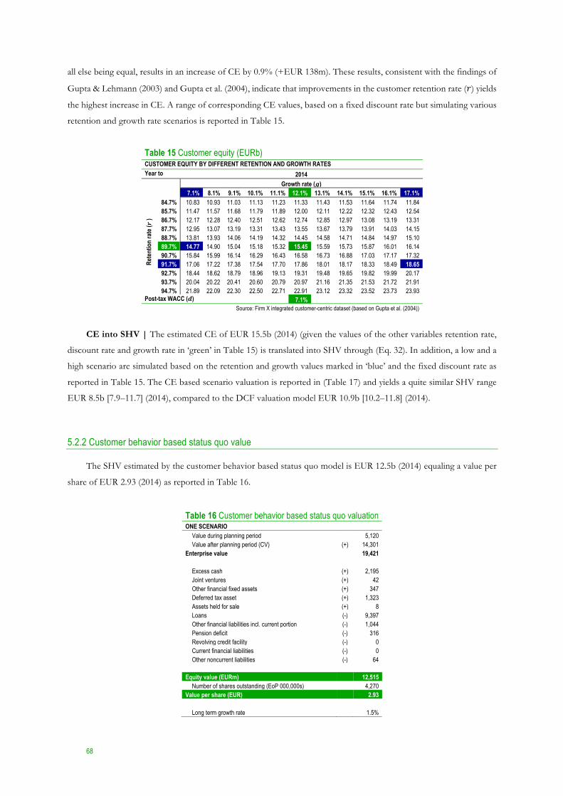
68

all else being equal, results in an increase of CE by 0.9% (+EUR 138m). These results, consistent with the findings of

Gupta & Lehmann (2003) and Gupta et al. (2004), indicate that improvements in the customer retention rate (!) yields

the highest increase in CE. A range of corresponding CE values, based on a fixed discount rate but simulating various

retention and growth rate scenarios is reported in Table 15.

Table 15 Customer equity (EURb) CUSTOMER EQUITY BY DIFFERENT RETENTION AND GROWTH RATES Year to 2014

Growth rate (à) 7.1% 8.1% 9.1% 10.1% 11.1% 12.1% 13.1% 14.1% 15.1% 16.1% 17.1%

Rete

ntio

n ra

te (â

)

84.7% 10.83 10.93 11.03 11.13 11.23 11.33 11.43 11.53 11.64 11.74 11.84 85.7% 11.47 11.57 11.68 11.79 11.89 12.00 12.11 12.22 12.32 12.43 12.54 86.7% 12.17 12.28 12.40 12.51 12.62 12.74 12.85 12.97 13.08 13.19 13.31 87.7% 12.95 13.07 13.19 13.31 13.43 13.55 13.67 13.79 13.91 14.03 14.15 88.7% 13.81 13.93 14.06 14.19 14.32 14.45 14.58 14.71 14.84 14.97 15.10 89.7% 14.77 14.90 15.04 15.18 15.32 15.45 15.59 15.73 15.87 16.01 16.14 90.7% 15.84 15.99 16.14 16.29 16.43 16.58 16.73 16.88 17.03 17.17 17.32 91.7% 17.06 17.22 17.38 17.54 17.70 17.86 18.01 18.17 18.33 18.49 18.65 92.7% 18.44 18.62 18.79 18.96 19.13 19.31 19.48 19.65 19.82 19.99 20.17 93.7% 20.04 20.22 20.41 20.60 20.79 20.97 21.16 21.35 21.53 21.72 21.91 94.7% 21.89 22.09 22.30 22.50 22.71 22.91 23.12 23.32 23.52 23.73 23.93

Post-tax WACC (ä) 7.1% Source: Firm X integrated customer-centric dataset (based on Gupta et al. (2004))

CE into SHV | The estimated CE of EUR 15.5b (2014) (given the values of the other variables retention rate,

discount rate and growth rate in ‘green’ in Table 15) is translated into SHV through (Eq. 32). In addition, a low and a

high scenario are simulated based on the retention and growth values marked in ‘blue’ and the fixed discount rate as

reported in Table 15. The CE based scenario valuation is reported in (Table 17) and yields a quite similar SHV range

EUR 8.5b [7.9–11.7] (2014), compared to the DCF valuation model EUR 10.9b [10.2–11.8] (2014).

5.2.2 Customer behavior based status quo value

The SHV estimated by the customer behavior based status quo model is EUR 12.5b (2014) equaling a value per

share of EUR 2.93 (2014) as reported in Table 16.

Table 16 Customer behavior based status quo valuation ONE SCENARIO

Value during planning period 5,120 Value after planning period (CV) (+) 14,301




Number of shares outstanding (EoP 000,000s) 4,270 Value per share (EUR) 2.93

Long term growth rate 1.5%

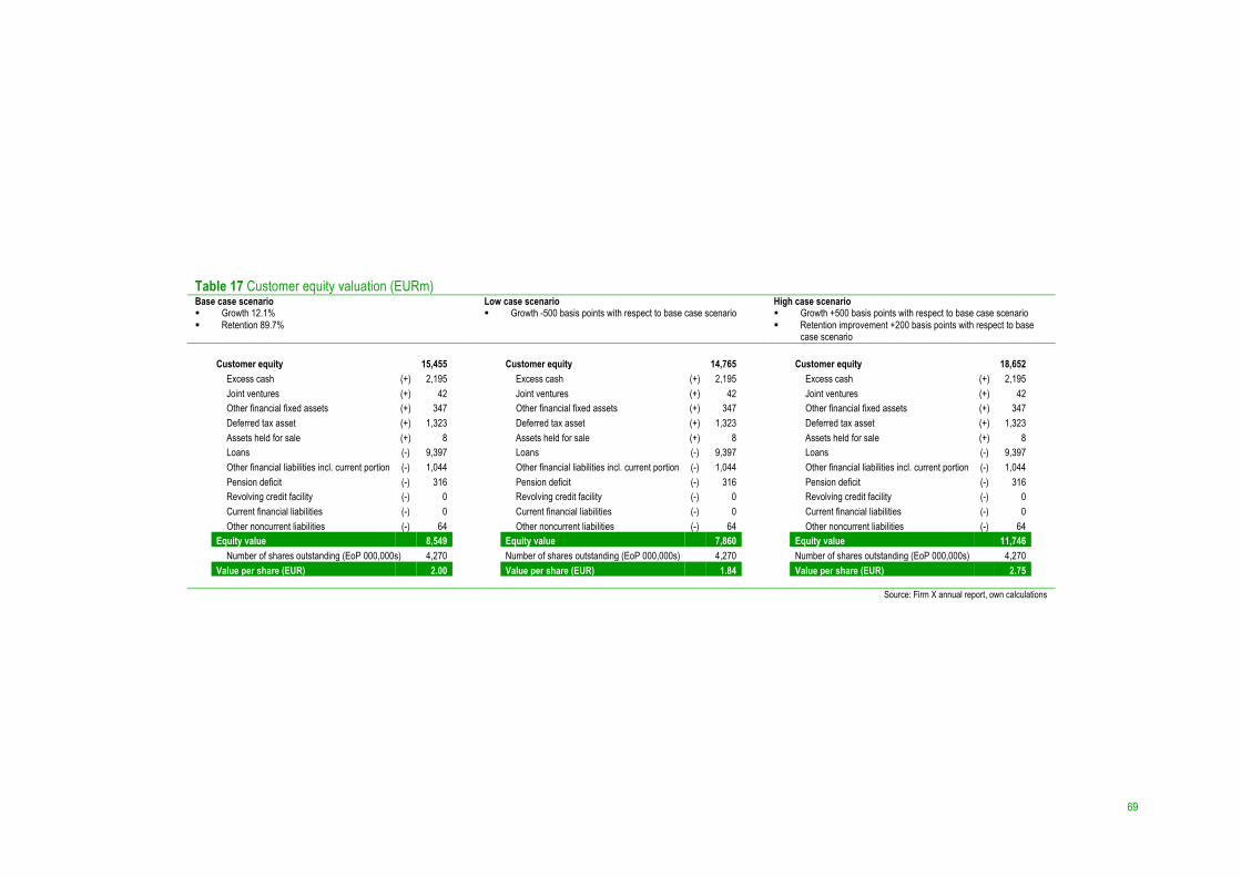
69

Table 17 Customer equity valuation (EURm) Base case scenario Low case scenario High case scenario § Growth 12.1% § Retention 89.7%

§ Growth -500 basis points with respect to base case scenario § Growth +500 basis points with respect to base case scenario § Retention improvement +200 basis points with respect to base

case scenario

Customer equity 15,455 Excess cash (+) 2,195 Joint ventures (+) 42 Other financial fixed assets (+) 347 Deferred tax asset (+) 1,323 Assets held for sale (+) 8 Loans (-) 9,397 Other financial liabilities incl. current portion (-) 1,044 Pension deficit (-) 316 Revolving credit facility (-) 0 Current financial liabilities (-) 0 Other noncurrent liabilities (-) 64

Equity value 8,549 Number of shares outstanding (EoP 000,000s) 4,270

Value per share (EUR) 2.00


Equity value 7,860 Number of shares outstanding (EoP 000,000s) 4,270 Value per share (EUR) 1.84


Equity value 11,746 Number of shares outstanding (EoP 000,000s) 4,270 Value per share (EUR) 2.75

Source: Firm X annual report, own calculations

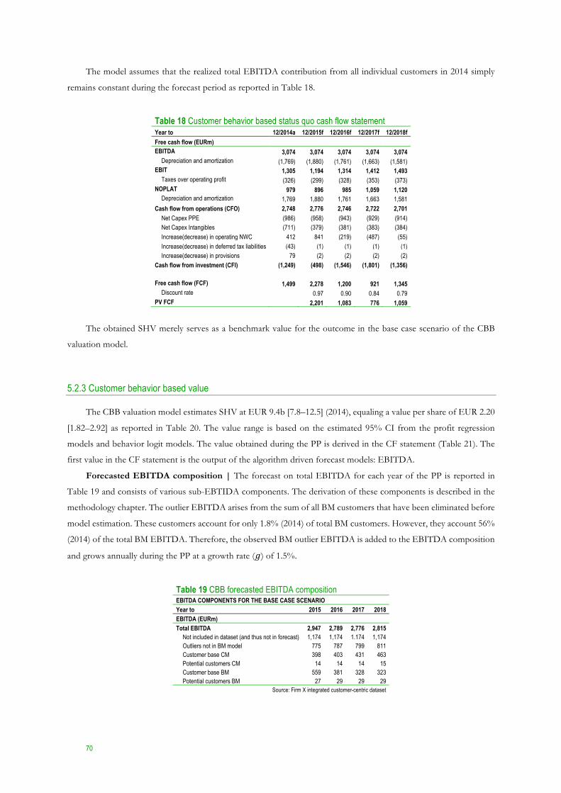
70

The model assumes that the realized total EBITDA contribution from all individual customers in 2014 simply

remains constant during the forecast period as reported in Table 18.

Table 18 Customer behavior based status quo cash flow statement Year to 12/2014a 12/2015f 12/2016f 12/2017f 12/2018f Free cash flow (EURm) EBITDA 3,074 3,074 3,074 3,074 3,074

Depreciation and amortization (1,769) (1,880) (1,761) (1,663) (1,581) EBIT 1,305 1,194 1,314 1,412 1,493

Taxes over operating profit (326) (299) (328) (353) (373) NOPLAT 979 896 985 1,059 1,120

Depreciation and amortization 1,769 1,880 1,761 1,663 1,581 Cash flow from operations (CFO) 2,748 2,776 2,746 2,722 2,701

Net Capex PPE (986) (958) (943) (929) (914) Net Capex Intangibles (711) (379) (381) (383) (384) Increase(decrease) in operating NWC 412 841 (219) (487) (55) Increase(decrease) in deferred tax liabilities (43) (1) (1) (1) (1) Increase(decrease) in provisions 79 (2) (2) (2) (2)

Cash flow from investment (CFI) (1,249) (498) (1,546) (1,801) (1,356)

Free cash flow (FCF) 1,499 2,278 1,200 921 1,345 Discount rate 0.97 0.90 0.84 0.79

PV FCF 2,201 1,083 776 1,059

The obtained SHV merely serves as a benchmark value for the outcome in the base case scenario of the CBB

valuation model.

5.2.3 Customer behavior based value

The CBB valuation model estimates SHV at EUR 9.4b [7.8–12.5] (2014), equaling a value per share of EUR 2.20

[1.82–2.92] as reported in Table 20. The value range is based on the estimated 95% CI from the profit regression

models and behavior logit models. The value obtained during the PP is derived in the CF statement (Table 21). The

first value in the CF statement is the output of the algorithm driven forecast models: EBITDA.

Forecasted EBITDA composition | The forecast on total EBITDA for each year of the PP is reported in

Table 19 and consists of various sub-EBTIDA components. The derivation of these components is described in the

methodology chapter. The outlier EBITDA arises from the sum of all BM customers that have been eliminated before

model estimation. These customers account for only 1.8% (2014) of total BM customers. However, they account 56%

(2014) of the total BM EBITDA. Therefore, the observed BM outlier EBITDA is added to the EBITDA composition

and grows annually during the PP at a growth rate (!) of 1.5%.

Table 19 CBB forecasted EBITDA composition EBITDA COMPONENTS FOR THE BASE CASE SCENARIO Year to 2015 2016 2017 2018 EBITDA (EURm) Total EBITDA 2,947 2,789 2,776 2,815

Not included in dataset (and thus not in forecast) 1,174 1,174 1.174 1,174 Outliers not in BM model 775 787 799 811 Customer base CM 398 403 431 463 Potential customers CM 14 14 14 15 Customer base BM 559 381 328 323 Potential customers BM 27 29 29 29


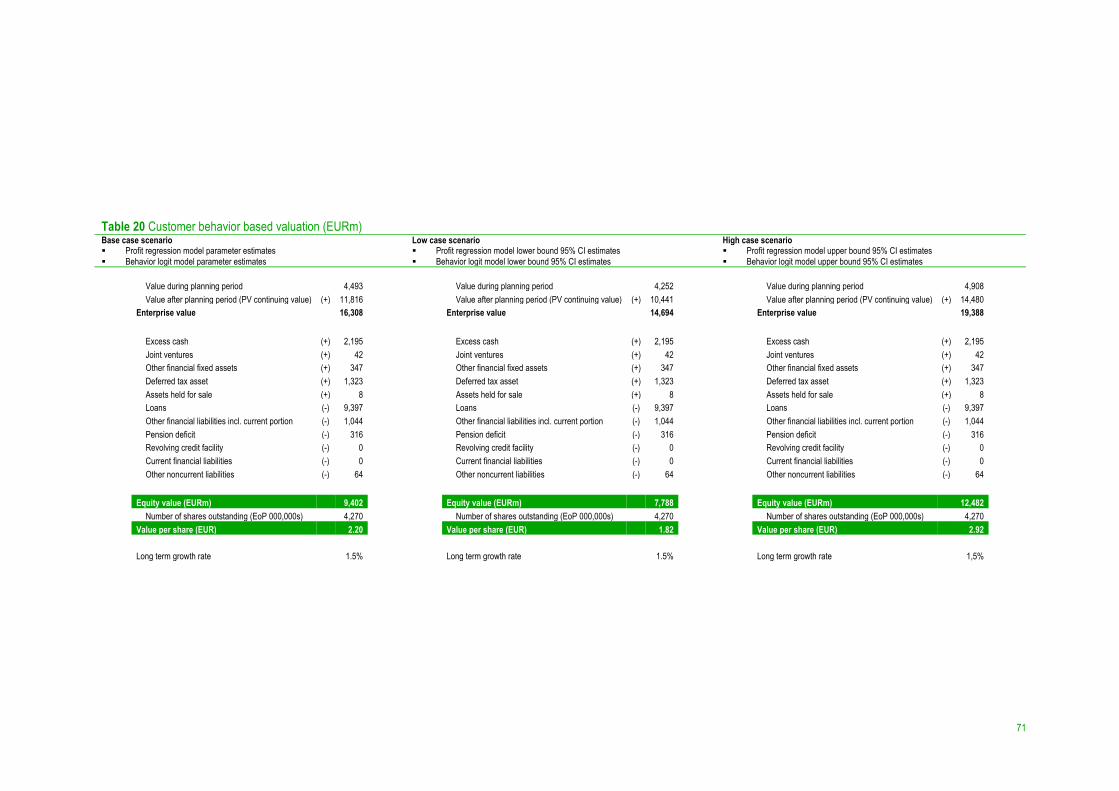
71

Table 20 Customer behavior based valuation (EURm) Base case scenario Low case scenario High case scenario § Profit regression model parameter estimates § Behavior logit model parameter estimates

§ Profit regression model lower bound 95% CI estimates § Behavior logit model lower bound 95% CI estimates

§ Profit regression model upper bound 95% CI estimates § Behavior logit model upper bound 95% CI estimates

Value during planning period 4,493 Value after planning period (PV continuing value) (+) 11,816




Number of shares outstanding (EoP 000,000s) 4,270 Value per share (EUR) 2.20 Long term growth rate 1.5%





Number of shares outstanding (EoP 000,000s) 4,270 Value per share (EUR) 1.82 Long term growth rate 1.5%





Number of shares outstanding (EoP 000,000s) 4,270 Value per share (EUR) 2.92 Long term growth rate 1,5%

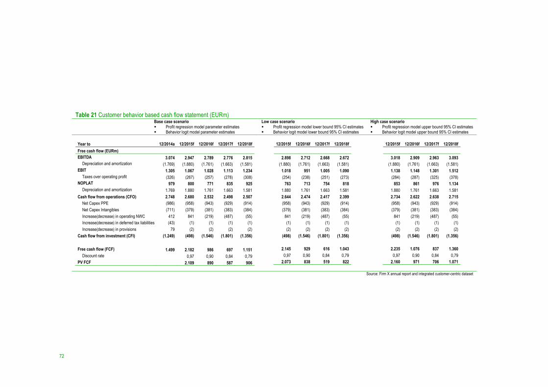
72

Table 21 Customer behavior based cash flow statement (EURm) Base case scenario Low case scenario High case scenario § Profit regression model parameter estimates

§ Behavior logit model parameter estimates § Profit regression model lower bound 95% CI estimates § Behavior logit model lower bound 95% CI estimates

§ Profit regression model upper bound 95% CI estimates § Behavior logit model upper bound 95% CI estimates

Year to 12/2014a 12/2015f 12/2016f 12/2017f 12/2018f Free cash flow (EURm) EBITDA 3.074 2.947 2.789 2.776 2.815

Depreciation and amortization (1.769) (1.880) (1.761) (1.663) (1.581) EBIT 1.305 1.067 1.028 1.113 1.234

Taxes over operating profit (326) (267) (257) (278) (308) NOPLAT 979 800 771 835 925

Depreciation and amortization 1.769 1.880 1.761 1.663 1.581 Cash flow from operations (CFO) 2.748 2.680 2.532 2.498 2.507

Net Capex PPE (986) (958) (943) (929) (914) Net Capex Intangibles (711) (379) (381) (383) (384) Increase(decrease) in operating NWC 412 841 (219) (487) (55) Increase(decrease) in deferred tax liabilities (43) (1) (1) (1) (1) Increase(decrease) in provisions 79 (2) (2) (2) (2)

Cash flow from investment (CFI) (1.249) (498) (1.546) (1.801) (1.356)

Free cash flow (FCF) 1.499 2.182 986 697 1.151 Discount rate 0,97 0,90 0,84 0,79

PV FCF 2.109 890 587 906

12/2015f 12/2016f 12/2017f 12/2018f

2.898 2.712 2.668 2.672 (1.880) (1.761) (1.663) (1.581)

1.018 951 1.005 1.090 (254) (238) (251) (273)

763 713 754 818 1.880 1.761 1.663 1.581 2.644 2.474 2.417 2.399 (958) (943) (929) (914) (379) (381) (383) (384)

841 (219) (487) (55) (1) (1) (1) (1) (2) (2) (2) (2)

(498) (1.546) (1.801) (1.356)

2.145 929 616 1.043 0,97 0,90 0,84 0,79

2.073 838 519 822

12/2015f 12/2016f 12/2017f 12/2018f

3.018 2.909 2.963 3.093 (1.880) (1.761) (1.663) (1.581)

1.138 1.148 1.301 1.512 (284) (287) (325) (378)

853 861 976 1.134 1.880 1.761 1.663 1.581 2.734 2.622 2.638 2.715 (958) (943) (929) (914) (379) (381) (383) (384)

841 (219) (487) (55) (1) (1) (1) (1) (2) (2) (2) (2)

(498) (1.546) (1.801) (1.356)

2.235 1.076 837 1.360 0,97 0,90 0,84 0,79

2.160 971 706 1.071

Source: Firm X annual report and integrated customer-centric dataset

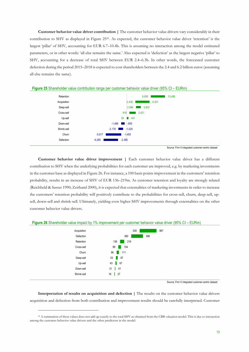
73

Customer behavior value driver contribution | The customer behavior value drivers vary considerably in their

contribution to SHV as displayed in Figure 2541. As expected, the customer behavior value driver ‘retention’ is the

largest ‘pillar’ of SHV, accounting for EUR 6.7–10.4b. This is assuming no interaction among the model estimated

parameters, or in other words: ‘all else remains the same.’ Also expected is ‘defection’ as the largest negative ‘pillar’ to

SHV, accounting for a decrease of total SHV between EUR 2.4–6.3b. In other words, the forecasted customer

defection during the period 2015–2018 is expected to cost shareholders between the 2.4 and 6.2 billion euros (assuming

all else remains the same).

Figure 25 Shareholder value contribution range per customer behavior value driver (95% CI – EURm)


Customer behavior value driver improvement | Each customer behavior value driver has a different

contribution to SHV when the underlying probabilities for each customer are improved, e.g. by marketing investments

in the customer base as displayed in Figure 26. For instance, a 100 basis points improvement in the customers’ retention

probability, results in an increase of SHV of EUR 136–219m. As customer retention and loyalty are strongly related

(Reichheld & Sasser 1990; Zeithaml 2000), it is expected that externalities of marketing investments in order to increase

the customers’ retention probability will positively contribute to the probabilities for cross-sell, churn, deep-sell, up-

sell, down-sell and shrink-sell. Ultimately, yielding even higher SHV improvements through externalities on the other

customer behavior value drivers.

Figure 26 Shareholder value impact by 1% improvement per customer behavior value driver (95% CI – EURm)


Interpretation of results on acquisition and defection | The results on the customer behavior value drivers

acquisition and defection from both contribution and improvement results should be carefully interpreted. Customer

41 A summation of these values does not add up exactly to the total SHV as obtained from the CBB valuation model. This is due to interaction

among the customer behavior value drivers and the other predictors in the model.

6,690

2,438

2,586

816

54

-605

-1,020

-1,493

-2,385

10,436

6,251

3,822

2,421

441

-1,466

-2,178

-5,617

-6,265

Retention

Acquisition

Deep-sell

Cross-sell

Up-sell

Down-sell

Shrink-sell

Churn

Defection

530

360

136

99

66

53

43

31

18

867

596

219

154

111

87

67

41

27

Acquisition

Defection

Retention

Cross-sell

Churn

Deep-sell

Up-sell

Down-sell

Shrink-sell

74

acquisition and defection are not ‘continuous’ processes and therefore cannot produce value throughout the years of

the PP. Once a customer is acquired it cannot be reacquired in the subsequent years, such that the probability value

after acquisition should go down to zero for these years. However, the probability of acquisition for potential

customers is very relevant. The inverse interpretation holds for defection.

5.2.3.1 Estimation results profit regression models

The parameter estimation results for the profit regression model is reported in Table 22 for CM and Table 23 for

BM.

Sign | All of the customer behavior value drivers (betas: 1–9) have the expected signs for both CM and BM models.

Retention, cross-sell, up-sell, deep-sell and acquisition have a positive sign. Therefore, a ‘unit’ increase in one of these

predictors increases a customer’s EBITDA contribution, hence profitability. Down-sell, shrink-sell, churn and

defection have a negative sign. Therefore, a ‘unit’ increase in one of these predictors decreases a customer’s EBITDA

contribution, hence profitability. Then, log EBITDA in the previous period (beta 10) has the expected sign for both CM

and BM models. Next, the customer relationship ages (betas: 11–21) reveal an interesting pattern. For CM year 1–7 and 10

have a negative sign, where year 8,9 and more than 10 have a positive sign. For BM year 1–8 have a negative sign,

where year 8, 9, 10 and more than 10 have a positive sign. Overall, having a relationship age above 8 years is positively

related to a customer’s EBITDA contribution. Finally, there is a large variety in signs among the customer characteristics

(betas: 22 and further).

Size | The logarithm transformation of the DV must be considered when interpreting the size of the estimated

parameters. The size interpretation for all the customer behavior value drivers are identical for both CM and BM model. For

instance, the CM model forecasts that a 1% increase in the customer’s retention probability, leads to an increase of log

EBITDA by 0.269% (beta 1). Where, in line with the findings of Schulze et al. (2012), for the CM and BM model the

size of ‘acquisition’ is the largest. Where for the CM model ‘shrink-sell’ and for the BM model ‘down-sell’ has the least

impact. The size interpretation for the log EBITDA in the previous period differs again as both DV and predictor have a

logarithm transformation. In this case the CM model forecasts that a 1% increase in the log EBITDA in the previous

period, leads to an increase of log EBITDA by 0.634% (beta 10). A possible explanation for this phenomenon is the

ongoing price pressure effect in the market42, which results in a customer repurchase with lower EBITDA contribution

compared to the previous contract. The same reasoning for interpretation applies to the BM model. The size

interpretation for the customer relationship ages are identical for both CM and BM model. For instance, the CM model

forecasts that a customer in its first year of the relationship with the firm, leads to a decrease in log EBITDA by 4.8%

(beta 11). The exact same holds for customers in their second year. In addition, these both effects are the largest among

the relationship age predictors. The size effect decreases from the third year onwards. A possible explanation is that

common contract periods in the industry last 1 or 2 years. The effect of relationship age decreases from the third year

onwards. Where the effect from 10 years of more is relatively large again (3.3%; beta 21). The same trend applies to

the BM results, but were the size in the first and second year are considerably larger, a decrease of 10.3% (beta 11) and

6.3% (beta 12) respectively. Finally, overall the sizes for the customer characteristics are relatively small for both the CM

and BM model.

42 Source: Firm X annual report 2014.

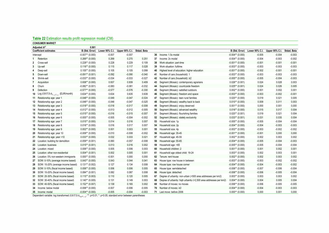
Table 22 Estimation results profit regression model (CM) CONSUMER MARKET Adjusted !" 0.901 Coefficient estimates B (Std. Error) Lower 95% C.I. Upper 95% C.I. Stdzd. Beta B (Std. Error) Lower 95% C.I. Upper 95% C.I. Stdzd. Beta Intercept -0.007** (0.000) -0.007 -0.007 36 Income: 1.5x modal -0.004** (0.000) -0.005 -0.004 -0.003 1 Retention 0.269** (0.000) 0.269 0.270 0.251 37 Income: 2x modal -0.004** (0.000) -0.004 -0.003 -0.002 2 Cross-sell 0.228** (0.000) 0.228 0.229 0.109 38 Work situation: part-time -0.001** (0.000) -0.001 -0.001 -0.001 3 Up-sell 0.116** (0.000) 0.115 0.117 0.028 39 Work situation: fulltime -0.003** (0.000) -0.003 -0.003 -0.003 4 Deep-sell 0.105** (0.000) 0.105 0.105 0.099 40 Highest level of education: higher education -0.001** (0.000) -0.002 -0.001 -0.001 5 Down-sell -0.091** (0.001) -0.092 -0.090 -0.040 41 Number of cars (household): 1 -0.003** (0.000) -0.003 -0.003 -0.003 6 Shrink-sell -0.033** (0.000) -0.034 -0.033 -0.027 42 Number of cars (household): ≥2 -0.005** (0.000) -0.005 -0.004 -0.003 7 Acquisition 0.938** (0.000) 0.937 0.939 0.409 43 Segment (Mosaic): contemporary agrarians 0.026** (0.001) 0.024 0.028 0.003 8 Churn -0.082** (0.001) -0.083 -0.081 -0.032 44 Segment (Mosaic): countryside freedom 0.025** (0.001) 0.024 0.026 0.005 9 Defection -0.577** (0.000) -0.577 -0.576 -0.330 45 Segment (Mosaic): satisfied outdoors 0.002** (0.000) 0.001 0.002 0.001 10 Log #$%&'()*+,)*- (EUR/month) 0.634** (0.000) 0.634 0.635 0.639 46 Segment (Mosaic): freedom and space -0.003** (0.000) -0.003 -0.002 -0.001 11 Relationship age: year 1 -0.048** (0.000) -0.049 -0.047 -0.024 47 Segment (Mosaic): teen rural families 0.020** (0.000) 0.019 0.021 0.005 12 Relationship age: year 2 -0.048** (0.000) -0.048 -0.047 -0.025 48 Segment (Mosaic): wealthy back to back 0.010** (0.000) 0.009 0.011 0.003 13 Relationship age: year 3 -0.018** (0.000) -0.018 -0.017 -0.008 49 Segment (Mosaic): enjoy deserved 0.001** (0.000) 0,000 0.001 0,000 14 Relationship age: year 4 -0.012** (0.000) -0.013 -0.012 -0.005 50 Segment (Mosaic): advanced wealthy 0.016** (0.000) 0.015 0.017 0.004 15 Relationship age: year 5 -0.015** (0.000) -0.016 -0.015 -0.007 51 Segment (Mosaic): flourishing families 0.020** (0.001) 0.019 0.021 0.004 16 Relationship age: year 6 -0.005** (0.000) -0.005 -0.004 -0.002 52 Segment (Mosaic): stately exclusivity 0.033** (0.001) 0.031 0.035 0.004 17 Relationship age: year 7 0.015** (0.000) 0.014 0.016 0.007 53 Household size: 1p -0.005** (0.000) -0.005 -0.004 -0.004 18 Relationship age: year 8 0.016** (0.000) 0.016 0.017 0.007 54 Household size: 2p -0.004** (0.000) -0.004 -0.003 -0.003 19 Relationship age: year 9 0.002** (0.000) 0.001 0.003 0.001 55 Household size: 4p -0.003** (0.000) -0.003 -0.002 -0.002 20 Relationship age: year 10 -0.009** (0.000) -0.010 -0.008 -0.002 56 Household age: 35-45 -0.001** (0.000) -0.001 0,000 0,000 21 Relationship age: year >10 0.033** (0.000) 0.032 0.033 0.021 57 Household age: 45-55 0.002** (0.000) 0.002 0.003 0.002 22 Location: building for demolition -0.059** (0.001) -0.060 -0.057 -0.008 58 Household age: 55-65 -0.004** (0.000) -0.005 -0.004 -0.003 23 Location: business 0.015** (0.001) 0.013 0.016 0.002 59 Household age: >65 -0.005** (0.000) -0.005 -0.004 -0.004 24 Location: mixed 0.006** (0.000) 0.005 0.006 0.003 60 Household children: 2 0.001** (0.000) 0.001 0.002 0.001 25 Location: other non-residential 0.004** (0.001) 0.002 0.005 0.001 61 Household age oldest child: 19-24 0.003** (0.000) 0.002 0.003 0.001 26 Location: 5% non-western immigrants 0.000** (0.000) -0.001 0,000 0,000 62 Tenure: rent house 0.002** (0.000) 0.002 0.003 0.002 27 SOW: 0-10% (average income based) 0.043** (0.000) 0.043 0.044 0.041 63 House type: row house in between -0.003** (0.000) -0.003 -0.002 -0.002 28 SOW: 10-20% (average income based) 0.131** (0.002) 0.127 0.134 0.008 64 House type: row house corner -0.004** (0.000) -0.004 -0.003 -0.002 29 SOW: 0-10% (fiscal income based) 0.006** (0.000) 0.006 0.006 0.005 65 House type: semidetached -0.006** (0.000) -0.007 -0.006 -0.004 30 SOW: 10-20% (fiscal income based) 0.084** (0.001) 0.082 0.087 0.008 66 House type: detached -0.006** (0.000) -0.006 -0.005 -0.004 31 SOW: 20-30% (fiscal income based) 0.115** (0.003) 0.110 0.120 0.005 67 Degree of urbanity: non-urban (<500 area addresses per km2) 0.003** (0.000) 0.003 0.003 0.002 32 SOW: 30-40% (fiscal income based) 0.140** (0.005) 0.131 0.149 0.003 68 Degree of urbanity: high urbanity (>2,500 area addresses per km2) 0.004** (0.000) 0.004 0.005 0.004 33 SOW: 40-50% (fiscal income based) 0.152** (0.007) 0.139 0.165 0.002 69 Number of moves: no moves -0.006** (0.000) -0.006 -0.005 -0.005 34 Income: below modal -0.006** (0.000) -0.007 -0.006 -0.005 70 Number of moves: ≥2 -0.004** (0.000) -0.004 -0.003 -0.003 35 Income: modal -0.004** (0.000) -0.005 -0.004 -0.003 71 Last move: before 2006 0.000** (0.000) 0,000 0.001 0,000 Dependent variable: log transformed #$%&'()/,)01; **: p<0.01; *: p<0.05; standard error between parentheses

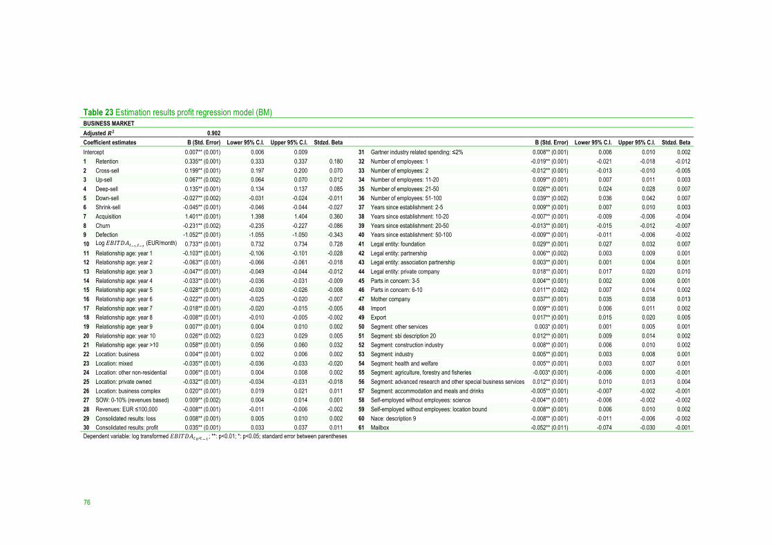
76

Table 23 Estimation results profit regression model (BM) BUSINESS MARKET Adjusted !" 0.902 Coefficient estimates B (Std. Error) Lower 95% C.I. Upper 95% C.I. Stdzd. Beta B (Std. Error) Lower 95% C.I. Upper 95% C.I. Stdzd. Beta Intercept 0.007** (0.001) 0.006 0.009 31 Gartner industry related spending: ≤2% 0.008** (0.001) 0.006 0.010 0.002 1 Retention 0.335** (0.001) 0.333 0.337 0.180 32 Number of employees: 1 -0.019** (0.001) -0.021 -0.018 -0.012 2 Cross-sell 0.199** (0.001) 0.197 0.200 0.070 33 Number of employees: 2 -0.012** (0.001) -0.013 -0.010 -0.005 3 Up-sell 0.067** (0.002) 0.064 0.070 0.012 34 Number of employees: 11-20 0.009** (0.001) 0.007 0.011 0.003 4 Deep-sell 0.135** (0.001) 0.134 0.137 0.085 35 Number of employees: 21-50 0.026** (0.001) 0.024 0.028 0.007 5 Down-sell -0.027** (0.002) -0.031 -0.024 -0.011 36 Number of employees: 51-100 0.039** (0.002) 0.036 0.042 0.007 6 Shrink-sell -0.045** (0.001) -0.046 -0.044 -0.027 37 Years since establishment: 2-5 0.009** (0.001) 0.007 0.010 0.003 7 Acquisition 1.401** (0.001) 1.398 1.404 0.360 38 Years since establishment: 10-20 -0.007** (0.001) -0.009 -0.006 -0.004 8 Churn -0.231** (0.002) -0.235 -0.227 -0.086 39 Years since establishment: 20-50 -0.013** (0.001) -0.015 -0.012 -0.007 9 Defection -1.052** (0.001) -1.055 -1.050 -0.343 40 Years since establishment: 50-100 -0.009** (0.001) -0.011 -0.006 -0.002 10 Log #$%&'()*+,)*- (EUR/month) 0.733** (0.001) 0.732 0.734 0.728 41 Legal entity: foundation 0.029** (0.001) 0.027 0.032 0.007 11 Relationship age: year 1 -0.103** (0.001) -0.106 -0.101 -0.028 42 Legal entity: partnership 0.006** (0.002) 0.003 0.009 0.001 12 Relationship age: year 2 -0.063** (0.001) -0.066 -0.061 -0.018 43 Legal entity: association partnership 0.003** (0.001) 0.001 0.004 0.001 13 Relationship age: year 3 -0.047** (0.001) -0.049 -0.044 -0.012 44 Legal entity: private company 0.018** (0.001) 0.017 0.020 0.010 14 Relationship age: year 4 -0.033** (0.001) -0.036 -0.031 -0.009 45 Parts in concern: 3-5 0.004** (0.001) 0.002 0.006 0.001 15 Relationship age: year 5 -0.028** (0.001) -0.030 -0.026 -0.008 46 Parts in concern: 6-10 0.011** (0.002) 0.007 0.014 0.002 16 Relationship age: year 6 -0.022** (0.001) -0.025 -0.020 -0.007 47 Mother company 0.037** (0.001) 0.035 0.038 0.013 17 Relationship age: year 7 -0.018** (0.001) -0.020 -0.015 -0.005 48 Import 0.009** (0.001) 0.006 0.011 0.002 18 Relationship age: year 8 -0.008** (0.001) -0.010 -0.005 -0.002 49 Export 0.017** (0.001) 0.015 0.020 0.005 19 Relationship age: year 9 0.007** (0.001) 0.004 0.010 0.002 50 Segment: other services 0.003* (0.001) 0.001 0.005 0.001 20 Relationship age: year 10 0.026** (0.002) 0.023 0.029 0.005 51 Segment: sbi description 20 0.012** (0.001) 0.009 0.014 0.002 21 Relationship age: year >10 0.058** (0.001) 0.056 0.060 0.032 52 Segment: construction industry 0.008** (0.001) 0.006 0.010 0.002 22 Location: business 0.004** (0.001) 0.002 0.006 0.002 53 Segment: industry 0.005** (0.001) 0.003 0.008 0.001 23 Location: mixed -0.035** (0.001) -0.036 -0.033 -0.020 54 Segment: health and welfare 0.005** (0.001) 0.003 0.007 0.001 24 Location: other non-residential 0.006** (0.001) 0.004 0.008 0.002 55 Segment: agriculture, forestry and fisheries -0.003* (0.001) -0.006 0.000 -0.001 25 Location: private owned -0.032** (0.001) -0.034 -0.031 -0.018 56 Segment: advanced research and other special business services 0.012** (0.001) 0.010 0.013 0.004 26 Location: business complex 0.020** (0.001) 0.019 0.021 0.011 57 Segment: accommodation and meals and drinks -0.005** (0.001) -0.007 -0.002 -0.001 27 SOW: 0-10% (revenues based) 0.009** (0.002) 0.004 0.014 0.001 58 Self-employed without employees: science -0.004** (0.001) -0.006 -0.002 -0.002 28 Revenues: EUR ≤100,000 -0.008** (0.001) -0.011 -0.006 -0.002 59 Self-employed without employees: location bound 0.008** (0.001) 0.006 0.010 0.002 29 Consolidated results: loss 0.008** (0.001) 0.005 0.010 0.002 60 Nace: description 9 -0.008** (0.001) -0.011 -0.006 -0.002 30 Consolidated results: profit 0.035** (0.001) 0.033 0.037 0.011 61 Mailbox -0.052** (0.011) -0.074 -0.030 -0.001 Dependent variable: log transformed #$%&'()/,)01; **: p<0.01; *: p<0.05; standard error between parentheses

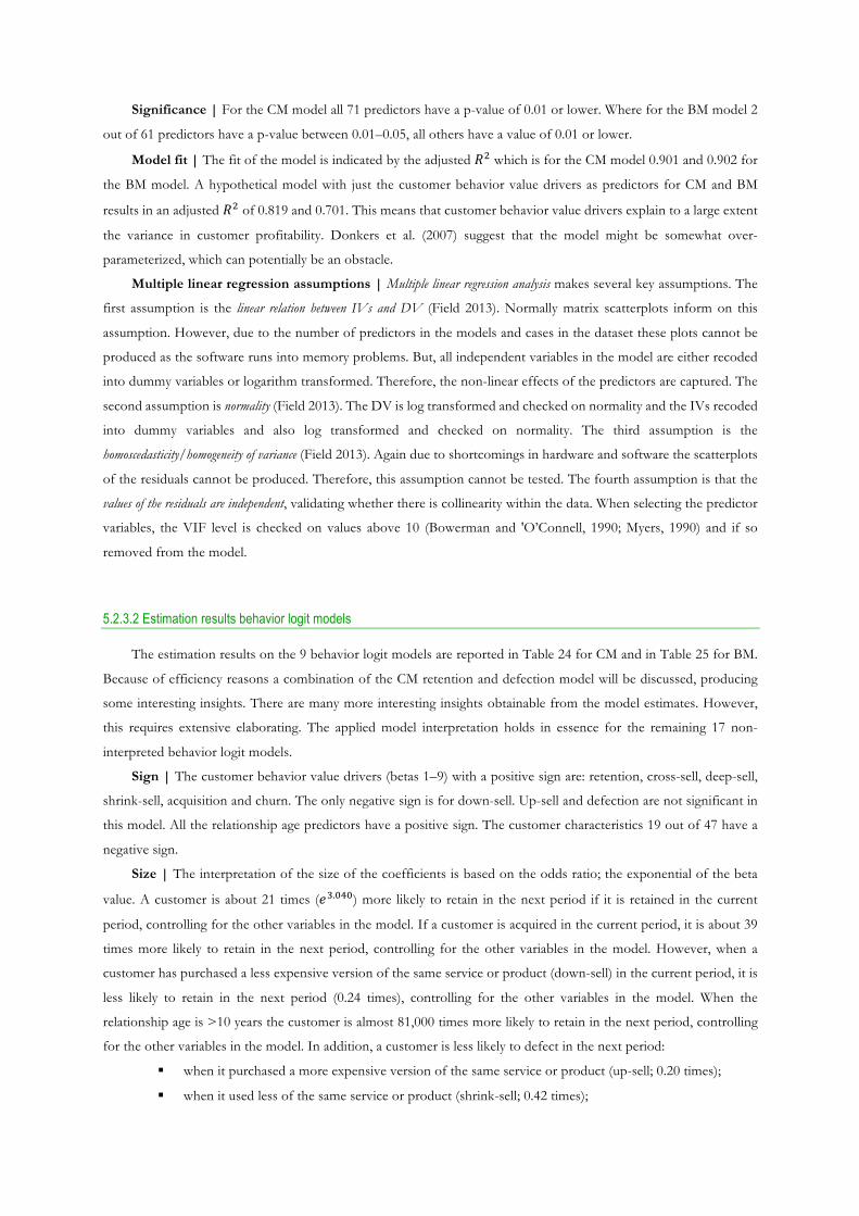
Significance | For the CM model all 71 predictors have a p-value of 0.01 or lower. Where for the BM model 2

out of 61 predictors have a p-value between 0.01–0.05, all others have a value of 0.01 or lower.

Model fit | The fit of the model is indicated by the adjusted !" which is for the CM model 0.901 and 0.902 for

the BM model. A hypothetical model with just the customer behavior value drivers as predictors for CM and BM

results in an adjusted !" of 0.819 and 0.701. This means that customer behavior value drivers explain to a large extent

the variance in customer profitability. Donkers et al. (2007) suggest that the model might be somewhat over-

parameterized, which can potentially be an obstacle.

Multiple linear regression assumptions | Multiple linear regression analysis makes several key assumptions. The

first assumption is the linear relation between IVs and DV (Field 2013). Normally matrix scatterplots inform on this

assumption. However, due to the number of predictors in the models and cases in the dataset these plots cannot be

produced as the software runs into memory problems. But, all independent variables in the model are either recoded

into dummy variables or logarithm transformed. Therefore, the non-linear effects of the predictors are captured. The

second assumption is normality (Field 2013). The DV is log transformed and checked on normality and the IVs recoded

into dummy variables and also log transformed and checked on normality. The third assumption is the

homoscedasticity/homogeneity of variance (Field 2013). Again due to shortcomings in hardware and software the scatterplots

of the residuals cannot be produced. Therefore, this assumption cannot be tested. The fourth assumption is that the

values of the residuals are independent, validating whether there is collinearity within the data. When selecting the predictor

variables, the VIF level is checked on values above 10 (Bowerman and 'O’Connell, 1990; Myers, 1990) and if so

removed from the model.

5.2.3.2 Estimation results behavior logit models

The estimation results on the 9 behavior logit models are reported in Table 24 for CM and in Table 25 for BM.

Because of efficiency reasons a combination of the CM retention and defection model will be discussed, producing

some interesting insights. There are many more interesting insights obtainable from the model estimates. However,

this requires extensive elaborating. The applied model interpretation holds in essence for the remaining 17 non-

interpreted behavior logit models.

Sign | The customer behavior value drivers (betas 1–9) with a positive sign are: retention, cross-sell, deep-sell,

shrink-sell, acquisition and churn. The only negative sign is for down-sell. Up-sell and defection are not significant in

this model. All the relationship age predictors have a positive sign. The customer characteristics 19 out of 47 have a

negative sign.

Size | The interpretation of the size of the coefficients is based on the odds ratio; the exponential of the beta

value. A customer is about 21 times (#$.&'&) more likely to retain in the next period if it is retained in the current

period, controlling for the other variables in the model. If a customer is acquired in the current period, it is about 39

times more likely to retain in the next period, controlling for the other variables in the model. However, when a

customer has purchased a less expensive version of the same service or product (down-sell) in the current period, it is

less likely to retain in the next period (0.24 times), controlling for the other variables in the model. When the

relationship age is >10 years the customer is almost 81,000 times more likely to retain in the next period, controlling

for the other variables in the model. In addition, a customer is less likely to defect in the next period:

§ when it purchased a more expensive version of the same service or product (up-sell; 0.20 times);

§ when it used less of the same service or product (shrink-sell; 0.42 times);

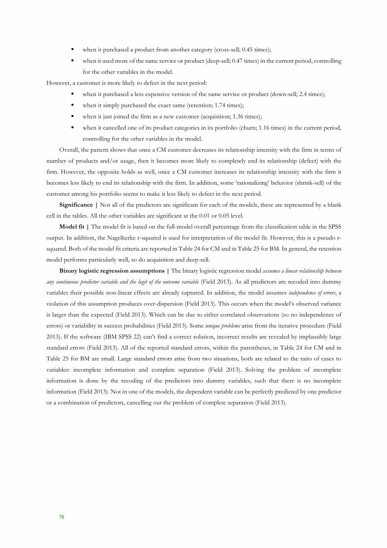
78

§ when it purchased a product from another category (cross-sell; 0.45 times);

§ when it used more of the same service or product (deep-sell; 0.47 times) in the current period, controlling

for the other variables in the model.

However, a customer is more likely to defect in the next period:

§ when it purchased a less expensive version of the same service or product (down-sell; 2.4 times);

§ when it simply purchased the exact same (retention; 1.74 times);

§ when it just joined the firm as a new customer (acquisition; 1.36 times);

§ when it cancelled one of its product categories in its portfolio (churn; 1.16 times) in the current period,

controlling for the other variables in the model.

Overall, the pattern shows that once a CM customer decreases its relationship intensity with the firm in terms of

number of products and/or usage, then it becomes more likely to completely end its relationship (defect) with the

firm. However, the opposite holds as well, once a CM customer increases its relationship intensity with the firm it

becomes less likely to end its relationship with the firm. In addition, some ‘rationalizing’ behavior (shrink-sell) of the

customer among his portfolio seems to make it less likely to defect in the next period.

Significance | Not all of the predictors are significant for each of the models, these are represented by a blank

cell in the tables. All the other variables are significant at the 0.01 or 0.05 level.

Model fit | The model fit is based on the full-model overall percentage from the classification table in the SPSS

output. In addition, the Nagelkerke r-squared is used for interpretation of the model fit. However, this is a pseudo r-

squared. Both of the model fit criteria are reported in Table 24 for CM and in Table 25 for BM. In general, the retention

model performs particularly well, so do acquisition and deep-sell.

Binary logistic regression assumptions | The binary logistic regression model assumes a linear relationship between

any continuous predictor variable and the logit of the outcome variable (Field 2013). As all predictors are recoded into dummy

variables their possible non-linear effects are already captured. In addition, the model assumes independence of errors, a

violation of this assumption produces over-dispersion (Field 2013). This occurs when the model’s observed variance

is larger than the expected (Field 2013). Which can be due to either correlated observations (so no independence of

errors) or variability in success probabilities (Field 2013). Some unique problems arise from the iterative procedure (Field

2013). If the software (IBM SPSS 22) can’t find a correct solution, incorrect results are revealed by implausibly large

standard errors (Field 2013). All of the reported standard errors, within the parentheses, in Table 24 for CM and in

Table 25 for BM are small. Large standard errors arise from two situations, both are related to the ratio of cases to

variables: incomplete information and complete separation (Field 2013). Solving the problem of incomplete

information is done by the recoding of the predictors into dummy variables, such that there is no incomplete

information (Field 2013). Not in one of the models, the dependent variable can be perfectly predicted by one predictor

or a combination of predictors, cancelling out the problem of complete separation (Field 2013).

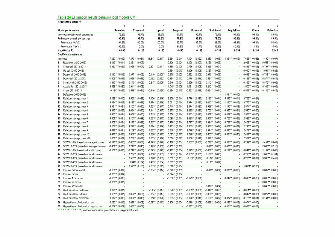
Table 24 Estimation results behavior logit models CM CONSUMER MARKET 1 2 3 4 5 6 7 8 9 Model performance Retention Cross-sell Up-sell Deep-sell Down-sell Shrink-sell Acquisition Churn Defection Intercept-model overall percentage 76,2% 93,7% 98,3% 51,9% 92,1% 75,1% 94,9% 93,6% 89.5% Full-model overall percentage 95.9% 93.7% 98.3% 77.9% 92.2% 79.0% 95.6% 93.6% 89.5%

Percentage 'No' (0) 94.2% 100.0% 100.0% 62.7% 99.9% 93.0% 98.6% 99.9% 100.0% Percentage 'Yes' (1) 96.5% 0.0% 0.0% 91.9% 1.7% 36.9% 40.4% 1.5% 0.0%

Nagelkerke R2 0.890 0.120 0.135 0.490 0.183 0.339 0.539 0.190 0.145 Coefficients estimates Intercept -7.057** (0.019) -7.373** (0.031) -11.847** (0.317) -5.664** (0.014) -7.124** (0.022) -6.383** (0.015) -4.821** (0.015) -7.626** (0.023) -1.490** (0.007) 1 Retention (2012-2013) 3.040** (0.014) 0.861** (0.007) - -0.106** (0.004) 1.498** (0.007) 1.159** (0.005) - 2.026** (0.009) 0.553** (0.004) 2 Cross-sell (2012-2013) 0.353** (0.023) -0.026** (0.007) 0.321** (0.011) 1.185** (0.006) 0.736** (0.005) 1.365** (0.004) - 0.815** (0.005) -0.797** (0.009) 3 Up-sell (l2012-2013) - - - -0.164** (0.010) 1.026** (0.009) 0.137** (0.009) - 0.040** (0.012) -1.591** (0.028) 4 Deep-sell (2012-2013) 0.142** (0.015) -0.377** (0.005) 0.419** (0.008) 0.575** (0.003) 0.562** (0.005) 0.970** (0.003) - 0.613** (0.005) -0.748** (0.005) 5 Down-sell (2012-2013) -1.409** (0.046) 0.096** (0.019) 0.162** (0.032) -0.194** (0.013) 0.178** (0.016) 0.584** (0.012) - 0.136** (0.018) 0.874** (0.014) 6 Shrink-sell (2012-2013) 1.810** (0.016) -0.140** (0.006) 0.347** (0.009) 0.646** (0.004) 0.359** (0.005) 0.142** (0.003) - 0.365** (0.005) -0.876** (0.006) 7 Acquisition (2012-2013) 3.668** (0.022) 0.941** (0.009) - 1.045** (0.006) 1.081** (0.009) 1.212** (0.006) - 1.500** (0.010) 0.306** (0.006) 8 Churn (2012-2013) 0.134* (0.055) 0.579** (0.021) -0.246** (0.038) -0.384** (0.015) -0.552** (0.019) -0.654** (0.014) - -0.559** (0.021) 0.145** (0.016) 9 Defection (2012-2013) - - - - - - 1.341** (0.010) - - 10 Relationship age: year 1 6.198** (0.015) 4.560** (0.029) 7.406** (0.316) 3.959** (0.014) 3.776** (0.020) 5.135** (0.014) 5.342** (0.011) 3.753** (0.021) - 11 Relationship age: year 2 9.994** (0.018) 4.127** (0.029) 7.974** (0.316) 6.061** (0.014) 3.974** (0.020) 4.413** (0.014) 1.190** (0.015) 3.773** (0.020) - 12 Relationship age: year 3 9.331** (0.021) 4.103** (0.030) 7.523** (0.317) 5.740** (0.014) 2.874** (0.020) 3.939** (0.014) 1.142** (0.019) 2.574** (0.020) - 13 Relationship age: year 4 9.317** (0.023) 4.034** (0.030) 7.441** (0.317) 5.975** (0.014) 2.825** (0.020) 3.752** (0.014) 0.935** (0.021) 2.545** (0.020) - 14 Relationship age: year 5 9.463** (0.024) 4.059** (0.030) 7.515** (0.317) 5.756** (0.014) 2.853** (0.020) 3.857** (0.014) 0.839** (0.022) 2.553** (0.020) - 15 Relationship age: year 6 9.458** (0.024) 4.105** (0.029) 7.523** (0.317) 5.590** (0.014) 2.825** (0.020) 3.867** (0.014) 0.762** (0.022) 2.528** (0.020) - 16 Relationship age: year 7 9.368** (0.024) 4.172** (0.029) 7.537** (0.317) 5.476** (0.014) 2.777** (0.020) 3.994** (0.014) 0.787** (0.022) 2.459** (0.020) - 17 Relationship age: year 8 9.056** (0.023) 4.220** (0.029) 7.524** (0.316) 6.163** (0.014) 2.555** (0.020) 3.930** (0.014) 0.662** (0.022) 2.215** (0.020) - 18 Relationship age: year 9 9.448** (0.034) 4.109** (0.030) 7.607** (0.317) 5.318** (0.015) 2.776** (0.021) 3.974** (0.015) 0.840** (0.032) 2.472** (0.022) - 19 Relationship age: year 10 9.472** (0.038) 3.987** (0.031) 7.588** (0.317) 5.523** (0.015) 2.728** (0.022) 3.855** (0.015) 0.831** (0.036) 2.427** (0.022) - 20 Relationship age: year >10 11.302** (0.022) 3.756** (0.029) 7.539** (0.316) 6.086** (0.013) 2.658** (0.019) 3.599** (0.014) - 2.389** (0.020) - 21 SOW 0-10% (based on average income) -0.110** (0.010) -0.685** (0.008) -1.275** (0.020) -0.466** (0.004) 0.137** (0.007) -0.218** (0.005) 0.331** (0.010) 0.299** (0.008) -1.451** (0.007) 22 SOW 10-20% (based on average income) -0.458** (0.071) 0.247** (0.043) 0.495** (0.052) -0.152** (0.037) - 0.081* (0.035) 0.438** (0.066) - -2.885** (0.210) 23 SOW 0-10% (based on fiscal income) -0.109** (0.010) -0.216** (0.008) -0.673** (0.022) -0.112** (0.004) 0.029** (0.007) -0.088** (0.005) 0.199** (0.010) 0.041** (0.008) -1.152** (0.008) 24 SOW 10-20% (based on fiscal income) - 0.754** (0.031) 2.358** (0.035) 0.697** (0.024) -0.205** (0.033) 0.138** (0.023) - -0.223** (0.036) -1.840** (0.101) 25 SOW 20-30% (based on fiscal income) - 0.551** (0.074) 2.396** (0.065) 0.832** (0.061) -0.168* (0.077) 0.132* (0.053) - -0.235** (0.089) -3.303** (0.449) 26 SOW 30-40% (based on fiscal income) - 0.341* (0.134) 2.465** (0.104) 0.882** (0.109) - 0.190* (0.092) - - - 27 SOW 40-50% (based on fiscal income) - 0.573** (0.180) 2.605** (0.143) 0.810** (0.154) - - - -0.621* (0.265) - 28 Income: below modal -0.166** (0.014) - -0.084** (0.014) -0.040** (0.005) - -0.011* (0.004) 0.076** (0.010) - 0.082** (0.006) 29 Income: modal -0.093** (0.012) - - -0.024** (0.004) - - - - - 30 Income: 1.5x modal -0.133** (0.013) - - -0.030** (0.005) -0.023** (0.006) - 0.044** (0.010) -0.018** (0.006) -0.033** (0.006) 31 Income: 2x modal -0.056** (0.011) - - - - - - - -0.063** (0.006) 32 Income: >2x modal - - - - - 0.010** (0.004) - - -0.046** (0.006) 33 Work situation: part time 0.078** (0.011) - -0.034* (0.017) 0.076** (0.005) -0.059** (0.008) -0.049** (0.005) - -0.061** (0.008) - 34 Work situation: full time 0.101** (0.011) -0.022** (0.006) -0.054** (0.017) 0.095** (0.005) -0.033** (0.008) -0.039** (0.005) - -0.047** (0.008) 0.027** (0.005) 35 Work situation: retirement 0.177** (0.016) -0.062** (0.010) -0.210** (0.020) 0.093** (0.007) -0.120** (0.010) -0.108** (0.007) 0.072** (0.013) -0.125** (0.011) 0.141** (0.005) 36 Highest level of education: low 0.080** (0.013) 0.028** (0.009) -0.077** (0.013) 0.106** (0.004) -0.079** (0.009) -0.039** (0.004) -0.036** (0.012) -0.074** (0.010) - 37 Highest level of education: high school -0.059** (0.009) 0.062** (0.007) - - -0.037** (0.007) - 0.051** (0.008) -0.035** (0.008) - **: p ≤ 0.01; *: p ≤ 0.05; standard error within parentheses; -: insignificant result

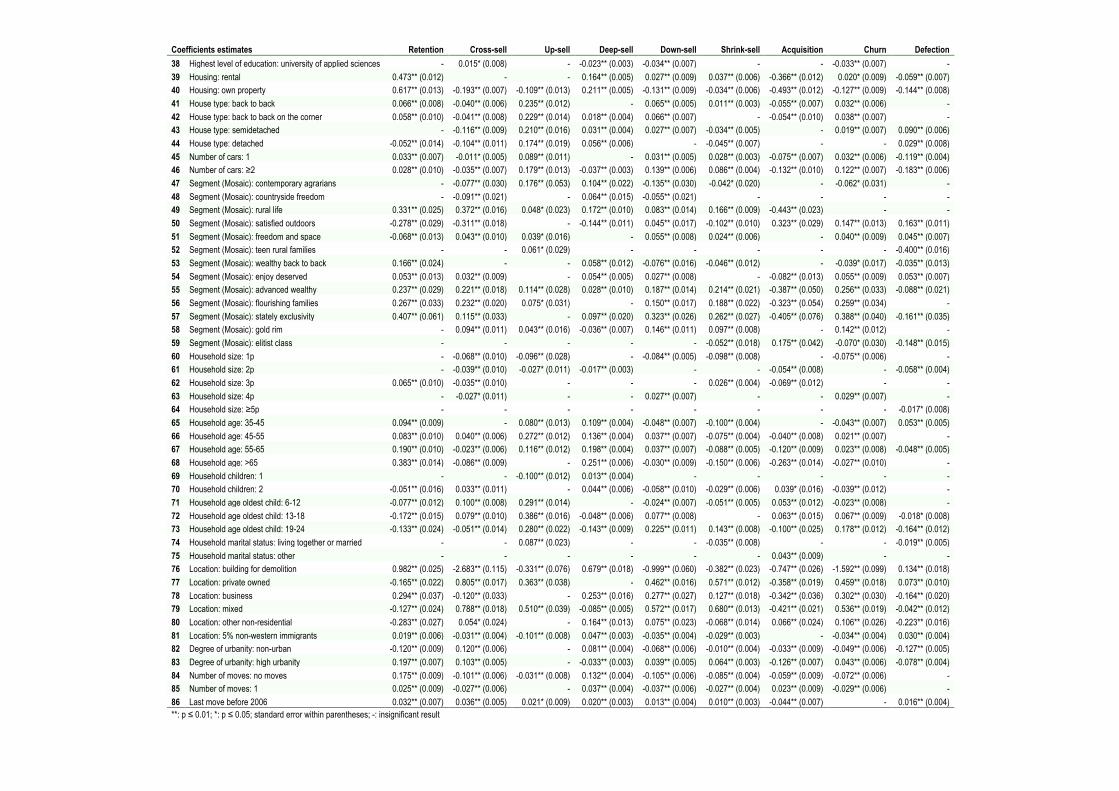
Coefficients estimates Retention Cross-sell Up-sell Deep-sell Down-sell Shrink-sell Acquisition Churn Defection 38 Highest level of education: university of applied sciences - 0.015* (0.008) - -0.023** (0.003) -0.034** (0.007) - - -0.033** (0.007) - 39 Housing: rental 0.473** (0.012) - - 0.164** (0.005) 0.027** (0.009) 0.037** (0.006) -0.366** (0.012) 0.020* (0.009) -0.059** (0.007) 40 Housing: own property 0.617** (0.013) -0.193** (0.007) -0.109** (0.013) 0.211** (0.005) -0.131** (0.009) -0.034** (0.006) -0.493** (0.012) -0.127** (0.009) -0.144** (0.008) 41 House type: back to back 0.066** (0.008) -0.040** (0.006) 0.235** (0.012) - 0.065** (0.005) 0.011** (0.003) -0.055** (0.007) 0.032** (0.006) - 42 House type: back to back on the corner 0.058** (0.010) -0.041** (0.008) 0.229** (0.014) 0.018** (0.004) 0.066** (0.007) - -0.054** (0.010) 0.038** (0.007) - 43 House type: semidetached - -0.116** (0.009) 0.210** (0.016) 0.031** (0.004) 0.027** (0.007) -0.034** (0.005) - 0.019** (0.007) 0.090** (0.006) 44 House type: detached -0.052** (0.014) -0.104** (0.011) 0.174** (0.019) 0.056** (0.006) - -0.045** (0.007) - - 0.029** (0.008) 45 Number of cars: 1 0.033** (0.007) -0.011* (0.005) 0.089** (0.011) - 0.031** (0.005) 0.028** (0.003) -0.075** (0.007) 0.032** (0.006) -0.119** (0.004) 46 Number of cars: ≥2 0.028** (0.010) -0.035** (0.007) 0.179** (0.013) -0.037** (0.003) 0.139** (0.006) 0.086** (0.004) -0.132** (0.010) 0.122** (0.007) -0.183** (0.006) 47 Segment (Mosaic): contemporary agrarians - -0.077** (0.030) 0.176** (0.053) 0.104** (0.022) -0.135** (0.030) -0.042* (0.020) - -0.062* (0.031) - 48 Segment (Mosaic): countryside freedom - -0.091** (0.021) - 0.064** (0.015) -0.055** (0.021) - - - - 49 Segment (Mosaic): rural life 0.331** (0.025) 0.372** (0.016) 0.048* (0.023) 0.172** (0.010) 0.083** (0.014) 0.166** (0.009) -0.443** (0.023) - - 50 Segment (Mosaic): satisfied outdoors -0.278** (0.029) -0.311** (0.018) - -0.144** (0.011) 0.045** (0.017) -0.102** (0.010) 0.323** (0.029) 0.147** (0.013) 0.163** (0.011) 51 Segment (Mosaic): freedom and space -0.068** (0.013) 0.043** (0.010) 0.039* (0.016) - 0.055** (0.008) 0.024** (0.006) - 0.040** (0.009) 0.045** (0.007) 52 Segment (Mosaic): teen rural families - - 0.061* (0.029) - - - - - -0.400** (0.016) 53 Segment (Mosaic): wealthy back to back 0.166** (0.024) - - 0.058** (0.012) -0.076** (0.016) -0.046** (0.012) - -0.039* (0.017) -0.035** (0.013) 54 Segment (Mosaic): enjoy deserved 0.053** (0.013) 0.032** (0.009) - 0.054** (0.005) 0.027** (0.008) - -0.082** (0.013) 0.055** (0.009) 0.053** (0.007) 55 Segment (Mosaic): advanced wealthy 0.237** (0.029) 0.221** (0.018) 0.114** (0.028) 0.028** (0.010) 0.187** (0.014) 0.214** (0.021) -0.387** (0.050) 0.256** (0.033) -0.088** (0.021) 56 Segment (Mosaic): flourishing families 0.267** (0.033) 0.232** (0.020) 0.075* (0.031) - 0.150** (0.017) 0.188** (0.022) -0.323** (0.054) 0.259** (0.034) - 57 Segment (Mosaic): stately exclusivity 0.407** (0.061) 0.115** (0.033) - 0.097** (0.020) 0.323** (0.026) 0.262** (0.027) -0.405** (0.076) 0.388** (0.040) -0.161** (0.035) 58 Segment (Mosaic): gold rim - 0.094** (0.011) 0.043** (0.016) -0.036** (0.007) 0.146** (0.011) 0.097** (0.008) - 0.142** (0.012) - 59 Segment (Mosaic): elitist class - - - - - -0.052** (0.018) 0.175** (0.042) -0.070* (0.030) -0.148** (0.015) 60 Household size: 1p - -0.068** (0.010) -0.096** (0.028) - -0.084** (0.005) -0.098** (0.008) - -0.075** (0.006) - 61 Household size: 2p - -0.039** (0.010) -0.027* (0.011) -0.017** (0.003) - - -0.054** (0.008) - -0.058** (0.004) 62 Household size: 3p 0.065** (0.010) -0.035** (0.010) - - - 0.026** (0.004) -0.069** (0.012) - - 63 Household size: 4p - -0.027* (0.011) - - 0.027** (0.007) - - 0.029** (0.007) - 64 Household size: ≥5p - - - - - - - - -0.017* (0.008) 65 Household age: 35-45 0.094** (0.009) - 0.080** (0.013) 0.109** (0.004) -0.048** (0.007) -0.100** (0.004) - -0.043** (0.007) 0.053** (0.005) 66 Household age: 45-55 0.083** (0.010) 0.040** (0.006) 0.272** (0.012) 0.136** (0.004) 0.037** (0.007) -0.075** (0.004) -0.040** (0.008) 0.021** (0.007) - 67 Household age: 55-65 0.190** (0.010) -0.023** (0.006) 0.116** (0.012) 0.198** (0.004) 0.037** (0.007) -0.088** (0.005) -0.120** (0.009) 0.023** (0.008) -0.048** (0.005) 68 Household age: >65 0.383** (0.014) -0.086** (0.009) - 0.251** (0.006) -0.030** (0.009) -0.150** (0.006) -0.263** (0.014) -0.027** (0.010) - 69 Household children: 1 - - -0.100** (0.012) 0.013** (0.004) - - - - - 70 Household children: 2 -0.051** (0.016) 0.033** (0.011) - 0.044** (0.006) -0.058** (0.010) -0.029** (0.006) 0.039* (0.016) -0.039** (0.012) - 71 Household age oldest child: 6-12 -0.077** (0.012) 0.100** (0.008) 0.291** (0.014) - -0.024** (0.007) -0.051** (0.005) 0.053** (0.012) -0.023** (0.008) - 72 Household age oldest child: 13-18 -0.172** (0.015) 0.079** (0.010) 0.386** (0.016) -0.048** (0.006) 0.077** (0.008) - 0.063** (0.015) 0.067** (0.009) -0.018* (0.008) 73 Household age oldest child: 19-24 -0.133** (0.024) -0.051** (0.014) 0.280** (0.022) -0.143** (0.009) 0.225** (0.011) 0.143** (0.008) -0.100** (0.025) 0.178** (0.012) -0.164** (0.012) 74 Household marital status: living together or married - - 0.087** (0.023) - - -0.035** (0.008) - - -0.019** (0.005) 75 Household marital status: other - - - - - - 0.043** (0.009) - - 76 Location: building for demolition 0.982** (0.025) -2.683** (0.115) -0.331** (0.076) 0.679** (0.018) -0.999** (0.060) -0.382** (0.023) -0.747** (0.026) -1.592** (0.099) 0.134** (0.018) 77 Location: private owned -0.165** (0.022) 0.805** (0.017) 0.363** (0.038) - 0.462** (0.016) 0.571** (0.012) -0.358** (0.019) 0.459** (0.018) 0.073** (0.010) 78 Location: business 0.294** (0.037) -0.120** (0.033) - 0.253** (0.016) 0.277** (0.027) 0.127** (0.018) -0.342** (0.036) 0.302** (0.030) -0.164** (0.020) 79 Location: mixed -0.127** (0.024) 0.788** (0.018) 0.510** (0.039) -0.085** (0.005) 0.572** (0.017) 0.680** (0.013) -0.421** (0.021) 0.536** (0.019) -0.042** (0.012) 80 Location: other non-residential -0.283** (0.027) 0.054* (0.024) - 0.164** (0.013) 0.075** (0.023) -0.068** (0.014) 0.066** (0.024) 0.106** (0.026) -0.223** (0.016) 81 Location: 5% non-western immigrants 0.019** (0.006) -0.031** (0.004) -0.101** (0.008) 0.047** (0.003) -0.035** (0.004) -0.029** (0.003) - -0.034** (0.004) 0.030** (0.004) 82 Degree of urbanity: non-urban -0.120** (0.009) 0.120** (0.006) - 0.081** (0.004) -0.068** (0.006) -0.010** (0.004) -0.033** (0.009) -0.049** (0.006) -0.127** (0.005) 83 Degree of urbanity: high urbanity 0.197** (0.007) 0.103** (0.005) - -0.033** (0.003) 0.039** (0.005) 0.064** (0.003) -0.126** (0.007) 0.043** (0.006) -0.078** (0.004) 84 Number of moves: no moves 0.175** (0.009) -0.101** (0.006) -0.031** (0.008) 0.132** (0.004) -0.105** (0.006) -0.085** (0.004) -0.059** (0.009) -0.072** (0.006) - 85 Number of moves: 1 0.025** (0.009) -0.027** (0.006) - 0.037** (0.004) -0.037** (0.006) -0.027** (0.004) 0.023** (0.009) -0.029** (0.006) - 86 Last move before 2006 0.032** (0.007) 0.036** (0.005) 0.021* (0.009) 0.020** (0.003) 0.013** (0.004) 0.010** (0.003) -0.044** (0.007) - 0.016** (0.004) **: p ≤ 0.01; *: p ≤ 0.05; standard error within parentheses; -: insignificant result

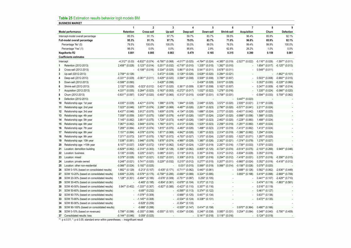
Table 25 Estimation results behavior logit models BM BUSINESS MARKET 1 2 3 4 5 6 7 8 9 Model performance Retention Cross-sell Up-sell Deep-sell Down-sell Shrink-sell Acquisition Churn Defection Intercept-model overall percentage 85.5% 91.1% 97.7% 59.7% 83.7% 59.5% 96.4% 85.9% 92.1% Full-model overall percentage 95.3% 91.1% 97.7% 79.5% 83.7% 71.0% 96.8% 85.9% 92.1%

Percentage 'No' (0) 79.5% 100.0% 100.0% 55.5% 99.5% 76.5% 99.4% 99.9% 100.0% Percentage 'Yes' (1) 98.0% 0.0% 0.0% 95.6% 2.9% 62.8% 26.2% 1.0% 0.0%

Nagelkerke R2 0.801 0.085 0.083 0.479 0.165 0.315 0.390 0.159 0.061 Coefficients estimates Intercept -4.312** (0.03) -6.832** (0.074) -6.790** (0.068) -4.017** (0.025) -4.764** (0.024) -4.385** (0.019) -2.527** (0.022) -5.116** (0.026) -1.597** (0.011) 1 Retention (2012-2013) 2.458** (0.028) 0.123** (0.014) 0.201** (0.032) -0.718** (0.010) 1.335** (0.015) 1.392** (0.010) - 1.654** (0.017) -0.125** (0.013) 2 Cross-sell (2012-2013) - -0.108** (0.016) 0.334** (0.025) 0.861** (0.014) 0.541** (0.011) 0.678** (0.011) - 0.549** (0.011) - 3 Up-sell (l2012-2013) 2.759** (0.126) - 0.472** (0.039) 0.126** (0.026) 0.628** (0.020) 0.284** (0.021) - - -1.662** (0.101) 4 Deep-sell (2012-2013) -0.331** (0.029) -0.061** (0.011) 0.429** (0.020) 0.594** (0.008) 0.509** (0.008) 0.789** (0.007) - 0.503** (0.008) -0.660** (0.015) 5 Down-sell (2012-2013) -0.599** (0.090) - 0.428** (0.056) - 0.436** (0.028) 0.610** (0.029) - 0.353** (0.030) -0.228** (0.060) 6 Shrink-sell (2012-2013) 2.132** (0.026) -0.023* (0.012) 0.421** (0.020) 0.361** (0.009) 0.381** (0.008) 0.162** (0.007) - 0.347** (0.009) -0.186** (0.014) 7 Acquisition (2012-2013) 4.331** (0.035) 0.264** (0.023) 0.163** (0.053) -0.272** (0.017) 1.032** (0.022) 1.276** (0.016) - 1.335** (0.024) -0.066** (0.020) 8 Churn (2012-2013) -0.831** (0.097) 0.243** (0.020) -0.493** (0.065) -0.313** (0.015) -0.638** (0.031) -0.758** (0.031) - -0.594** (0.033) 0.759** (0.062) 9 Defection (2012-2013) - - - - - - 0.447** (0.023) - - 10 Relationship age: 1st year 4.035** (0.028) 4.421** (0.074) 1.586** (0.078) 1.944** (0.028) 2.048** (0.025) 3.572** (0.020) 2.935** (0.021) 2.119** (0.026) - 11 Relationship age: 2nd year 7.023** (0.046) 3.877** (0.074) 2.288** (0.069) 4.487** (0.026) 2.261** (0.023) 2.790** (0.020) -0.571** (0.041) 2.211** (0.024) - 12 Relationship age: 3rd year 6.437** (0.046) 3.912** (0.075) 1.609** (0.076) 4.134** (0.026) 1.686** (0.024) 2.773** (0.020) -0.401** (0.042) 1.629** (0.025) - 13 Relationship age: 4th year 7.059** (0.059) 3.931** (0.075) 1.656** (0.076) 4.416** (0.026) 1.637** (0.024) 2.524** (0.020) -0.998** (0.056) 1.588** (0.025) - 14 Relationship age: 5th year 7.145** (0.062) 3.951** (0.075) 1.729** (0.073) 4.440** (0.026) 1.545** (0.023) 2.463** (0.020) -1.228** (0.060) 1.488** (0.024) - 15 Relationship age: 6th year 7.067** (0.062) 3.949** (0.074) 1.760** (0.071) 4.413** (0.026) 1.525** (0.023) 2.256** (0.019) -1.281** (0.060) 1.455** (0.024) - 16 Relationship age: 7th year 7.269** (0.064) 4.013** (0.074) 1.815** (0.070) 4.483** (0.026) 1.498** (0.023) 2.316** (0.019) -1.413** (0.062) 1.413** (0.024) - 17 Relationship age: 8th year 7.151** (0.064) 4.078** (0.074) 1.871** (0.069) 4.842** (0.026) 1.387** (0.023) 2.314** (0.019) -1.386** (0.062) 1.294** (0.024) - 18 Relationship age: 9th year 7.371** (0.073) 3.977** (0.075) 1.782** (0.072) 4.753** (0.027) 1.370** (0.024) 2.230** (0.020) -1.522** (0.071) 1.287** (0.025) - 19 Relationship age: 10th year 7.538** (0.081) 3.946** (0.076) 1.878** (0.074) 4.990** (0.028) 1.380** (0.026) 2.352** (0.021) -1.374** (0.079) 1.276** (0.027) - 20 Relationship age: >10th year 8.107** (0.037) 3.828** (0.072) 1.916** (0.062) 5.402** (0.024) 1.225** (0.019) 2.287** (0.016) -1.739** (0.033) 1.079** (0.020) - 21 Location: demolition building -0.829** (0.062) -2.314** (0.303) 1.538** (0.126) 0.356** (0.062) -0.805** (0.125) -0.724** (0.074) -0.514** (0.075) -2.103** (0.269) 0.949** (0.046) 22 Location: business 0.135** (0.026) 0.225** (0.021) 0.085** (0.031) 0.118** (0.013) 0.357** (0.016) 0.312** (0.012) -0.834** (0.029) 0.353** (0.016) - 23 Location: mixed 0.379** (0.026) 0.621** (0.021) 0.332** (0.031) 0.306** (0.013) 0.329** (0.016) 0.294** (0.012) -1.416** (0.031) 0.375** (0.016) -0.356** (0.015) 24 Location: private owned 0.248** (0.021) 0.741** (0.020) 0.229** (0.032) 0.215** (0.012) 0.277** (0.015) 0.207** (0.011) -0.865** (0.024) 0.352** (0.016) -0.418** (0.012) 25 Location: other non-residential -0.066** (0.024) 0.192** (0.025) - 0.031* (0.015) 0.069** (0.019) 0.066** (0.014) -0.156** (0.026) 0.079** (0.020) - 26 SOW 0-10% (based on consolidated results) 1.882** (0.129) -0.213* (0.107) -0.435* (0.171) -0.711** (0.062) 0.440** (0.061) - 0.688** (0.126) 0.582** (0.062) -2.636** (0.449) 27 SOW 10-20% (based on consolidated results) 0.606** (0.205) -0.579** (0.175) -0.758** (0.285) -0.690** (0.089) 0.324** (0.095) - 0.855** (0.198) 0.419** (0.098) -2.669** (0.709) 28 SOW 20-30% (based on consolidated results) 1.128** (0.351) -0.494** (0.185) -0.676* (0.309) -0.751** (0.097) 0.250* (0.105) - - 0.441** (0.107) -2.429** (0.710) 29 SOW 30-40% (based on consolidated results) - -0.465* (0.195) -0.804* (0.361) -0.678** (0.104) 0.373** (0.112) - - 0.474** (0.116) -1.883** (0.581) 30 SOW 40-50% (based on consolidated results) 0.847* (0.402) -1.333** (0.307) -0.827* (0.385) -0.423** (0.110) 0.357** (0.116) - - 0.516** (0.119) - 31 SOW 50-60% (based on consolidated results) - -0.69** (0.232) - -0.595** (0.113) 0.374** (0.122) - - 0.461** (0.127) - 32 SOW 60-70% (based on consolidated results) - -1.079** (0.309) - -0.668** (0.125) 0.457** (0.134) - - 0.637** (0.136) - 33 SOW 70-80% (based on consolidated results) - -1.145** (0.308) - -0.534** (0.124) 0.338** (0.131) - - 0.472** (0.135) - 34 SOW 80-90% (based on consolidated results) - -0.628* (0.259) - -0.354** (0.133) - - - - - 35 SOW 90-100% (based on consolidated results) - -0.688* (0.288) - -0.529** (0.147) 0.414** (0.158) - 0.970** (0.364) 0.480** (0.166) - 36 SOW 0-10% (based on revenues) 0.799** (0.096) -0.355** (0.066) -0.555** (0.101) -0.554** (0.036) 0.246** (0.038) 0.085** (0.031) 0.254** (0.094) 0.348** (0.040) -3.790** (0.409) 37 Consolidated results: loss -0.144** (0.046) 0.059* (0.025) - - 0.141** (0.018) 0.118** (0.016) - 0.124** (0.019) - **: p ≤ 0.01; *: p ≤ 0.05; standard error within parentheses; -: insignificant result

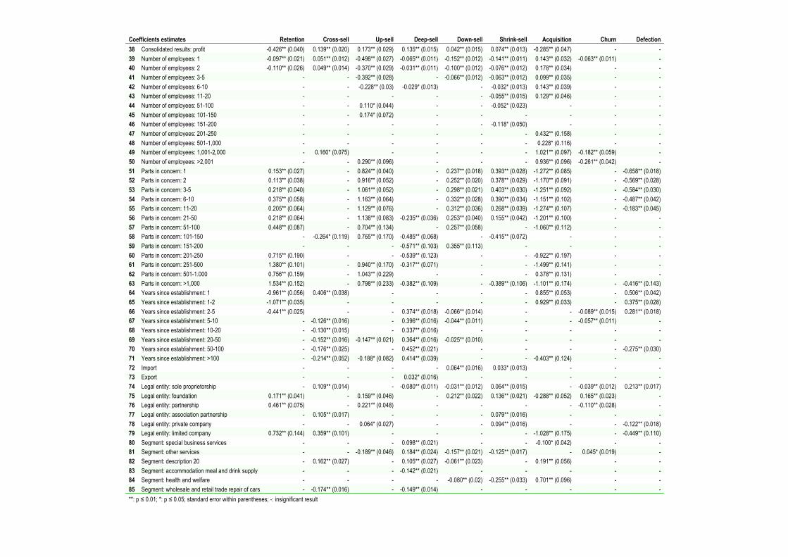
Coefficients estimates Retention Cross-sell Up-sell Deep-sell Down-sell Shrink-sell Acquisition Churn Defection 38 Consolidated results: profit -0.426** (0.040) 0.139** (0.020) 0.173** (0.029) 0.135** (0.015) 0.042** (0.015) 0.074** (0.013) -0.285** (0.047) - - 39 Number of employees: 1 -0.097** (0.021) 0.051** (0.012) -0.498** (0.027) -0.065** (0.011) -0.152** (0.012) -0.141** (0.011) 0.143** (0.032) -0.063** (0.011) - 40 Number of employees: 2 -0.110** (0.026) 0.049** (0.014) -0.370** (0.029) -0.031** (0.011) -0.100** (0.012) -0.076** (0.012) 0.178** (0.034) - - 41 Number of employees: 3-5 - - -0.392** (0.028) - -0.066** (0.012) -0.063** (0.012) 0.099** (0.035) - - 42 Number of employees: 6-10 - - -0.228** (0.03) -0.029* (0.013) - -0.032* (0.013) 0.143** (0.039) - - 43 Number of employees: 11-20 - - - - - -0.055** (0.015) 0.129** (0.046) - - 44 Number of employees: 51-100 - - 0.110* (0.044) - - -0.052* (0.023) - - - 45 Number of employees: 101-150 - - 0.174* (0.072) - - - - - - 46 Number of employees: 151-200 - - - - - -0.118* (0.050) - - - 47 Number of employees: 201-250 - - - - - - 0.432** (0.158) - - 48 Number of employees: 501-1,000 - - - - - - 0.228* (0.116) - - 49 Number of employees: 1,001-2,000 - 0.160* (0.075) - - - - 1.021** (0.097) -0.182** (0.059) - 50 Number of employees: >2,001 - - 0.290** (0.096) - - - 0.936** (0.096) -0.261** (0.042) - 51 Parts in concern: 1 0.153** (0.027) - 0.824** (0.040) - 0.237** (0.018) 0.393** (0.028) -1.272** (0.085) - -0.658** (0.018) 52 Parts in concern: 2 0.113** (0.038) - 0.916** (0.052) - 0.252** (0.020) 0.378** (0.029) -1.170** (0.091) - -0.569** (0.028) 53 Parts in concern: 3-5 0.218** (0.040) - 1.061** (0.052) - 0.298** (0.021) 0.403** (0.030) -1.251** (0.092) - -0.584** (0.030) 54 Parts in concern: 6-10 0.375** (0.058) - 1.163** (0.064) - 0.332** (0.028) 0.390** (0.034) -1.151** (0.102) - -0.487** (0.042) 55 Parts in concern: 11-20 0.205** (0.064) - 1.129** (0.076) - 0.312** (0.036) 0.268** (0.039) -1.274** (0.107) - -0.183** (0.045) 56 Parts in concern: 21-50 0.218** (0.064) - 1.138** (0.083) -0.235** (0.036) 0.253** (0.040) 0.155** (0.042) -1.201** (0.100) - - 57 Parts in concern: 51-100 0.448** (0.087) - 0.704** (0.134) - 0.257** (0.058) - -1.060** (0.112) - - 58 Parts in concern: 101-150 - -0.264* (0.119) 0.765** (0.170) -0.485** (0.068) - -0.415** (0.072) - - - 59 Parts in concern: 151-200 - - - -0.571** (0.103) 0.355** (0.113) - - - - 60 Parts in concern: 201-250 0.715** (0.190) - - -0.539** (0.123) - - -0.922** (0.197) - - 61 Parts in concern: 251-500 1.380** (0.101) - 0.940** (0.170) -0.317** (0.071) - - -1.499** (0.141) - - 62 Parts in concern: 501-1.000 0.756** (0.159) - 1.043** (0.229) - - - 0.378** (0.131) - - 63 Parts in concern: >1,000 1.534** (0.152) - 0.798** (0.233) -0.382** (0.109) - -0.389** (0.106) -1.101** (0.174) - -0.416** (0.143) 64 Years since establishment: 1 -0.961** (0.056) 0.406** (0.038) - - - - 0.855** (0.053) - 0.506** (0.042) 65 Years since establishment: 1-2 -1.071** (0.035) - - - - - 0.929** (0.033) - 0.375** (0.028) 66 Years since establishment: 2-5 -0.441** (0.025) - - 0.374** (0.018) -0.066** (0.014) - - -0.089** (0.015) 0.281** (0.018) 67 Years since establishment: 5-10 - -0.126** (0.016) - 0.396** (0.016) -0.044** (0.011) - - -0.057** (0.011) - 68 Years since establishment: 10-20 - -0.130** (0.015) - 0.337** (0.016) - - - - - 69 Years since establishment: 20-50 - -0.152** (0.016) -0.147** (0.021) 0.364** (0.016) -0.025** (0.010) - - - - 70 Years since establishment: 50-100 - -0.176** (0.025) - 0.452** (0.021) - - - - -0.275** (0.030) 71 Years since establishment: >100 - -0.214** (0.052) -0.188* (0.082) 0.414** (0.039) - - -0.403** (0.124) - - 72 Import - - - - 0.064** (0.016) 0.033* (0.013) - - - 73 Export - - - 0.032* (0.016) - - - - - 74 Legal entity: sole proprietorship - 0.109** (0.014) - -0.080** (0.011) -0.031** (0.012) 0.064** (0.015) - -0.039** (0.012) 0.213** (0.017) 75 Legal entity: foundation 0.171** (0.041) - 0.159** (0.046) - 0.212** (0.022) 0.136** (0.021) -0.288** (0.052) 0.165** (0.023) - 76 Legal entity: partnership 0.461** (0.075) - 0.221** (0.048) - - - - -0.110** (0.028) - 77 Legal entity: association partnership - 0.105** (0.017) - - - 0.079** (0.016) - - - 78 Legal entity: private company - - 0.064* (0.027) - - 0.094** (0.016) - - -0.122** (0.018) 79 Legal entity: limited company 0.732** (0.144) 0.359** (0.101) - - - - -1.028** (0.175) - -0.449** (0.110) 80 Segment: special business services - - - 0.098** (0.021) - - -0.100* (0.042) - - 81 Segment: other services - - -0.189** (0.046) 0.184** (0.024) -0.157** (0.021) -0.125** (0.017) - 0.045* (0.019) - 82 Segment: description 20 - 0.162** (0.027) - 0.105** (0.027) -0.061** (0.023) - 0.191** (0.056) - - 83 Segment: accommodation meal and drink supply - - - -0.142** (0.021) - - - - - 84 Segment: health and welfare - - - - -0.080** (0.02) -0.255** (0.033) 0.701** (0.096) - - 85 Segment: wholesale and retail trade repair of cars - -0.174** (0.016) - -0.149** (0.014) - - - - - **: p ≤ 0.01; *: p ≤ 0.05; standard error within parentheses; -: insignificant result

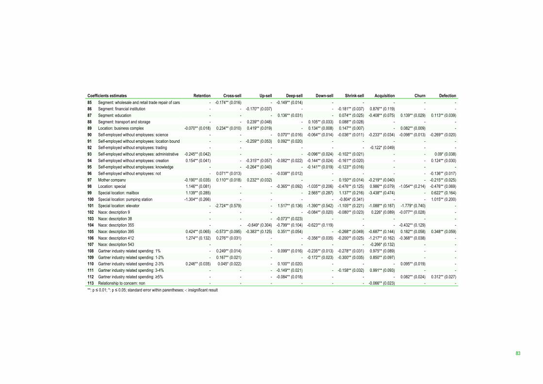
83

Coefficients estimates Retention Cross-sell Up-sell Deep-sell Down-sell Shrink-sell Acquisition Churn Defection 85 Segment: wholesale and retail trade repair of cars - -0.174** (0.016) - -0.149** (0.014) - - - - - 86 Segment: financial institution - - -0.170** (0.037) - - -0.181** (0.037) 0.876** (0.119) - - 87 Segment: education - - - 0.136** (0.031) - 0.074** (0.025) -0.408** (0.075) 0.139** (0.029) 0.113** (0.039) 88 Segment: transport and storage - - 0.239** (0.048) - 0.105** (0.033) 0.088** (0.028) - - - 89 Location: business complex -0.070** (0.018) 0.234** (0.010) 0.419** (0.019) - 0.134** (0.008) 0.147** (0.007) - 0.082** (0.009) - 90 Self-employed without employees: science - - - 0.070** (0.016) -0.064** (0.014) -0.036** (0.011) -0.233** (0.034) -0.098** (0.013) -0.269** (0.020) 91 Self-employed without employees: location bound - - -0.259** (0.053) 0.092** (0.020) - - - - - 92 Self-employed without employees: trading - - - - - - -0.122* (0.049) - - 93 Self-employed without employees: administrative -0.245** (0.042) - - - -0.096** (0.024) -0.102** (0.021) - - 0.09* (0.038) 94 Self-employed without employees: creation 0.154** (0.041) - -0.315** (0.057) -0.082** (0.022) -0.144** (0.024) -0.161** (0.020) - - 0.124** (0.030) 95 Self-employed without employees: knowledge - - -0.264** (0.040) - -0.141** (0.019) -0.123** (0.016) - - - 96 Self-employed without employees: not - 0.071** (0.013) - -0.038** (0.012) - - - - -0.136** (0.017) 97 Mother company -0.190** (0.035) 0.110** (0.018) 0.232** (0.032) - - 0.150** (0.014) -0.219** (0.040) - -0.215** (0.025) 98 Location: special 1.146** (0.081) - - -0.365** (0.092) -1.035** (0.206) -0.476** (0.125) 0.986** (0.079) -1.054** (0.214) -0.476** (0.069) 99 Special location: mailbox 1.139** (0.285) - - - 2.565** (0.287) 1.137** (0.216) -3.438** (0.474) - 0.622** (0.164) 100 Special location: pumping station -1.304** (0.266) - - - - -0.804* (0.341) - - 1.015** (0.200) 101 Special location: elevator - -2.724** (0.579) - 1.517** (0.136) -1.390** (0.542) -1.105** (0.221) -1.088** (0.187) -1.779* (0.740) - 102 Nace: description 9 - - - - -0.084** (0.020) -0.080** (0.023) 0.226* (0.089) -0.077** (0.028) - 103 Nace: description 38 - - - -0.073** (0.023) - - - - - 104 Nace: description 355 - - -0.649* (0.304) -0.799** (0.104) -0.623** (0.119) - - -0.432** (0.129) - 105 Nace: description 395 0.424** (0.065) -0.573** (0.095) -0.383** (0.125) 0.351** (0.054) - -0.268** (0.049) -0.687** (0.144) 0.182** (0.058) 0.348** (0.059) 106 Nace: description 412 1.274** (0.132) 0.276** (0.031) - - -0.356** (0.035) -0.200** (0.025) -1.217** (0.162) -0.368** (0.038) - 107 Nace: description 543 - - - - - - -0.266* (0.132) - - 108 Gartner industry related spending: 1% - 0.249** (0.014) - 0.099** (0.016) -0.235** (0.013) -0.278** (0.031) 0.975** (0.089) - - 109 Gartner industry related spending: 1-2% - 0.167** (0.021) - - -0.172** (0.023) -0.300** (0.035) 0.850** (0.097) - - 110 Gartner industry related spending: 2-3% 0.246** (0.035) 0.045* (0.022) - 0.100** (0.020) - - - 0.095** (0.019) - 111 Gartner industry related spending: 3-4% - - - -0.149** (0.021) - -0.158** (0.032) 0.991** (0.093) - - 112 Gartner industry related spending: ≥5% - - - -0.084** (0.018) - - - 0.082** (0.024) 0.312** (0.027) 113 Relationship to concern: non - - - - - - -0.066** (0.023) - - **: p ≤ 0.01; *: p ≤ 0.05; standard error within parentheses; -: insignificant result

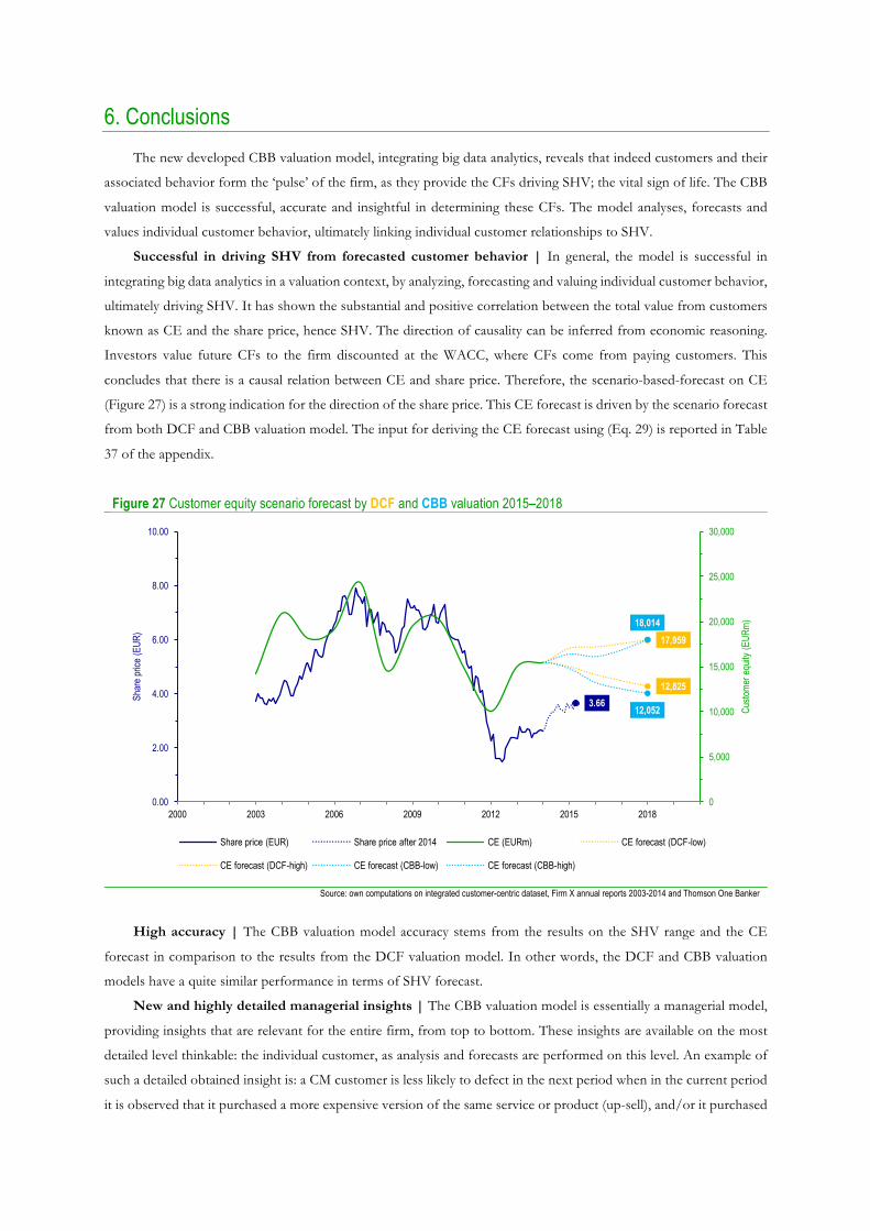
6. Conclusions The new developed CBB valuation model, integrating big data analytics, reveals that indeed customers and their

associated behavior form the ‘pulse’ of the firm, as they provide the CFs driving SHV; the vital sign of life. The CBB

valuation model is successful, accurate and insightful in determining these CFs. The model analyses, forecasts and

values individual customer behavior, ultimately linking individual customer relationships to SHV.

Successful in driving SHV from forecasted customer behavior | In general, the model is successful in

integrating big data analytics in a valuation context, by analyzing, forecasting and valuing individual customer behavior,

ultimately driving SHV. It has shown the substantial and positive correlation between the total value from customers

known as CE and the share price, hence SHV. The direction of causality can be inferred from economic reasoning.

Investors value future CFs to the firm discounted at the WACC, where CFs come from paying customers. This

concludes that there is a causal relation between CE and share price. Therefore, the scenario-based-forecast on CE

(Figure 27) is a strong indication for the direction of the share price. This CE forecast is driven by the scenario forecast

from both DCF and CBB valuation model. The input for deriving the CE forecast using (Eq. 29) is reported in Table

37 of the appendix.

Figure 27 Customer equity scenario forecast by DCF and CBB valuation 2015–2018

Source: own computations on integrated customer-centric dataset, Firm X annual reports 2003-2014 and Thomson One Banker

High accuracy | The CBB valuation model accuracy stems from the results on the SHV range and the CE

forecast in comparison to the results from the DCF valuation model. In other words, the DCF and CBB valuation

models have a quite similar performance in terms of SHV forecast.

New and highly detailed managerial insights | The CBB valuation model is essentially a managerial model,

providing insights that are relevant for the entire firm, from top to bottom. These insights are available on the most

detailed level thinkable: the individual customer, as analysis and forecasts are performed on this level. An example of

such a detailed obtained insight is: a CM customer is less likely to defect in the next period when in the current period

it is observed that it purchased a more expensive version of the same service or product (up-sell), and/or it purchased

3.6612,825

17,959

12,052

18,014

0

5,000

10,000

15,000

20,000

25,000

30,000

0.00

2.00

4.00

6.00

8.00

10.00

2000 2003 2006 2009 2012 2015 2018

Custo

mer e

quity

(EUR

m)

Shar

e pric

e (E

UR)

Share price (EUR) Share price after 2014 CE (EURm) CE forecast (DCF-low)

CE forecast (DCF-high) CE forecast (CBB-low) CE forecast (CBB-high)

85

a product from another category (cross-sell), and/or it used more of the same service or product (deep-sell).43

However, a CM customer is more likely to defect in the next period when in the current period it is observed that it

purchased a less expensive version of the same service or product, and/or it simply purchased the exact same

(retention; 1.74 times more like to defect), and/or it just joined the firm as a new customer (acquisition; 1.36 times

more likely), and/ or it cancelled one of its product categories in its portfolio. Yet another detailed insight that can be

obtained from the CBB valuation model is the ranking of individual customer values or e.g. ranked cross-sell

probabilities; the likeliness a customer is going to cross-buy from the firm. However, this is out of the scope of this

study, and is merely an example to illustrate its performance on new and detailed insights. This highly detailed level of

information enables managers to estimate ROIC and growth on the individual customer level. Ultimately, the model

provides insights that support budget allocation on the individual customer level. This provides managers with the

ability to manage customer relationships based on their estimated future value contribution. Or in other words, the

model supports managers to seek for the upside potential on the individual customer level.

6.1 Hypotheses testing

A summary on the results of the tested hypotheses is reported in Table 26. Different models have been used in

testing these hypotheses. The results on the hypotheses related to the customer behavior value drivers from the CBB

valuation model, is in accordance with the empirical findings.

Table 26 Summary of hypotheses-testing results

Hypotheses Significant (CM; BM)

Sign (CM; BM)

Result (CM; BM)

1 The value per share estimated by DCF valuation, approximates the price per share. n/a n/a EUR 2.56 versus 2.63 2 CE and share price are positively correlated. * (+) !"= 0.695 3 Improvements in the retention rate affects CE. ** (+) accepted 4 The EV estimated by DCF valuation, approximates CE estimated by CE valuation. n/a n/a EUR 17.8b versus 15.5b 5 Customer purchase behavior explains the variance in customer profitability. n/a n/a !"= 0.819; !"= 0.701 6 There is a positive relation between retention and customer profitability. **; ** (+; +) accepted; accepted 7 There is a positive relation between cross-sell and customer profitability. **; ** (+; +) accepted; accepted 8 There is a positive relation between up-sell and customer profitability. **; ** (+; +) accepted; accepted 9 There is a positive relation between deep-sell and customer profitability. **; ** (+; +) accepted; accepted

10 There is a negative relation between down-sell and customer profitability. **; ** (–; –) accepted; accepted 11 There is a negative relation between shrink-sell and customer profitability. **; ** (–; –) accepted; accepted 12 There is a positive relation between acquisition and customer profitability. **; ** (+; +) accepted; accepted 13 There is a negative relation between churn and customer profitability. **; ** (–; –) accepted; accepted 14 There is a negative relation between defection and customer profitability. **; ** (–; –) accepted; accepted 15 Observed customer behavior affects future customer behavior. ~ (±; ±) accepted; accepted 16 Customer brand choice affects customer behavior. n/a n/a n/a 17 Customer brand choice affects customer profitability. n/a n/a n/a 18 Customer characteristics affect customer behavior. ~ (±; ±) accepted; accepted 19 Customer characteristics affect customer profitability. ~ (±; ±) accepted; accepted 20 Relationship age affects customer purchase behavior. **; ** (±; ±) accepted; accepted 21 There is a positive relation between relationship age and customer profitability. **; ** (±; ±) accepted; accepted 22 Share of wallet affects customer purchase-behavior. ~ (±; ±) accepted; accepted 23 There is a positive relation between share of wallet and customer profitability. ~ (±; ±) accepted; accepted **: p ≤ 0.01; *: p ≤ 0.05; n/a: not applicable; ~: various variables significant but on different levels; ±: both signs are applicable; /: ambiguous results

In an attempt to bridge the gap between quantitative marketing and finance, this study leveraged big data analytics

as the connective tissue in a firm valuation context. An accurate CF forecast is vital to a proper valuation. Big data

analytics, applied in a such a context, has the potential to increase the forecast accuracy. The new insights and

43 Controlling for other variables in the model.

86

forthcoming applications from this valuation model has the potential to create significant SHV. The model enables

senior executives to conduct value relevant data driven decision making. Resulting in better strategies that provide the

firm with competitive advantages that drives price premiums and efficient capital use, thus increasing ROIC and

growth, hence SHV.

SHV is driven by a chain of value drivers, where incremental CFs discounted at the firm’s WACC is the most

primary source of SHV creation. The right balance between ROIC and revenue growth is critical for the increase in

CFs. Improvements in ROIC and growth are driven by the firm’s competitive advantage resulting from its strategy.

The DCF valuation methodology is the most common used methodology in determining SHV, relying solely on CFs

in and out of the firm. The forecast on the breakdown into price and volume components of key value drivers is based

on the analyst’s personal view. The DCF valuation model estimated value per share is EUR 2.56 and approximates the

price per share EUR 2.63 (H1).

Empirical studies in marketing have shown its substantial contribution to SHV. This follows logically on the fact

that marketing is all about building the intangible assets of the firm. The firm’s most important intangible asset are its

customers, and needs to be valued accordingly. The recently emerged CBV literature in marketing sees customers as

assets and makes them the central object of analysis and valuation. Empirical studies in CBV is built up around the

CLV concept showing that the sum of all CLVs, known as CE, is a good proxy for the EV. The correlation between

CE and the historical share price is 0.695 (H2). CLV and CE models are based on customer margins, retention rates,

acquisition costs and a discount rate. An improvement of 100 basis points in the retention rate increases CE by 7.3%

(H3). The level of EV EUR 17.8b estimated by the DCF valuation model approximates the level of CE EUR 15.5b

estimated by the CE valuation model (H4). Individual customer behavior drives CLV and improvements in CE are

linked to improvements in SHV, equals individual customer behavior drives SHV. The variance in customer

profitability is largely (CM !"=0.819; BM !"=0.701) explained by individual customer purchase behavior (H5). Nine

customer behavior value drivers are significantly related to the forecast of customer profitability, hence SHV, for both

CM and BM the signs are identical, thus accepting all related hypotheses: retention (positive, H6), cross-sell (positive,

H7), up-sell (positive, H8), deep-sell (H9), down-sell (negative, H10), shrink-sell (negative, H11), acquisition (positive,

H12), churn (negative, H13) and defection (negative, H14). In addition, in order to forecast several periods ahead a

forecast on observed customer behavior is required. As a result, observed customer behavior forecasts future behavior

and drives customer profitability, hence SHV (H15). Customers derive value from brands and as a result it drives their

loyalty. Increases in customer loyalty drives the firms price premium, and results in incremental CFs to the firm, hence

SHV. However, as the impact of brands on SHV is recognized it was not possible to incorporate these effects in the

model. Due to serious shortcomings in software and hardware specifications44 it is highly recommended to run the

model, and similar analysis on a server. Incorporating these effects would have increased the number of behavior logit

models to be estimated from 18 (2 segments; 9 behaviors) to 72 (2 segments; 9 behaviors; 4 brands), increasing the

computed probabilities from 2 to 18 billion, resulting in an estimated 1TB of data. This is simply impossible. Therefore,

these brand effects have not been tested, thus the hypotheses (H16 and H17) are not applicable. Then, customer

characteristics are related to customer needs and tastes, linking customer characteristics to the purchase decision

process. It follows that customer characteristics support in the forecast of customer behavior (H18) and customer

profitability (H19) for both CM and BM models. Another variable supporting in forecasting is the customer’s

relationship age. When the customer relationship age with the firm increases, it also increases its: loyalty, retention

44 IBM SPSS Statistics 22 (software); Intel i7 + 4GB memory + Windows 7 32-bits and Intel i5 + 16GB memory + SSD + OSX 64-bits

87

probability, satisfaction and switching costs. In general, the customer relationship age affects its behavior (H20). In

addition, it affects customer profitability as well. For early years in the relationship, the direction of the relation is

negative, where for later years this becomes positive for both CM and BM models. However, its profitability increases

as the relationship age increases, as the negative parameter decreases in size (H21). The final variable supporting in

forecasting is share of wallet (SOW). When the customer’s SOW increases, it also increases its loyalty. Therefore, the

customer’s SOW affects its behavior (H22). In addition, it affects customer profitability as well. However, the direction

of the relation is ambiguous for both CM and BM customers (H23).

6.2 Comparing DCF and CBB valuation models

A summary of the comparison between DCF and CBB valuation models, revealing the differences and similarities,

is reported in Table 27.

Common goal different forecast model | Both DCF and CBB valuation models aim to forecast SHV and

result in very similar values. The SHV range from the DCF valuation model falls within the range of the CBB valuation

model. The last value range, is a result from low- and high scenarios based on the lower and upper estimated 95% CI

bounds. An objective approach in scenario analysis. However, the DCF low- and high scenario values, result from the

analyst’s view on the development of the breakdown into price and volume components of the key- and operating

value drivers. These are drivers are driven by its understanding of the firm’s industry dynamics and its competitive

position and strategy. Clearly a more subjective approach in scenario analysis.

Different value driver setup | Both DCF and CBB valuation models have a similar value driver setup, however

the value drivers themselves are completely different. The value drivers for the DCF valuation model are more product-

centric oriented where for the CBB valuation model this is customer-centric oriented. In essence, this setup makes

both models two sides of the same coin.

Different analysis approach | Due to the value driver setup both DCF and CBB valuation models have a

different approach in analysis. Where the CBB valuation model is clearly an ‘inside-out’ analysis approach the DCF

valuation model has a more ambiguous approach, but essentially is more ‘outside-in.’

Different insights | DCF and CBB valuation models provide very different insights. The DCF valuation model

insights are mainly on the line item level of the P&L and BS. This provides an overview on for instance, the forecasted

revenue growth, EBITDA, EBITDA-margin, CAPEX, NWC, tax-rate and FCF. The development of these items are

considered all highly relevant to firm value. However, the CBB valuation model delivers insights on the level of

individual customer relationship with the firm. It forecasts future behavior, based on observed behavior, providing

insights for instance like: “a customer is less likely to defect in the next period, even though it is observed that it uses

less of the same service or product (shrink-sell) during the current period.” This detailed insight could be explained as

that there is a group of customers (CM) that at first seems to be less engaged with the firm based on their decreased

usage and therefore may leave the firm. However, against all odds the results show that they are less likely to leave.

This could indicate a more rational type of customer. In general, these kinds of detailed insights can serve as valuable

input in developing strategies, tactics and policies, targeted to ‘similar behaving’ customers or customer-cohorts, in

order to stimulate certain customer behavior, thus maximize individual profitability, hence SHV. Based on the different

value driver setup and analysis approach, very similar results in valuation, and very different insights it can be concluded

that both models are therefore complementary to each other.

88

Table 27 Comparing DCF and CBB valuation model DISCOUNTED CASH FLOW VALUATION MODEL CUSTOMER BEHAVIOR BASED VALUATION MODEL DATA

Availability / accessibility

§ Publicly available financial data incl. KPIs § Datastreams, annual reports etc.

§ Big data (internal) § Integrated customer-centric dataset (new developed)

Usability § Readily available for analysis § Extensive data collection § Extensive data preparation

Variables All variables (line items) from: § Balance sheet § Profit & loss § Cash flow statement § Additional KPIs

Variables (±1,500) from an integrated customer-centric dataset: § Revenues per BSP combination § EBITDA margin (%) on BSP level § Customer behavior (derived) § Product ownership (derived) § Brand (4 different) § Segments (2 different) § Products (29 different) § Number of customers on location § Various customer characteristics (CM and BM)

Level of aggregation

§ Firm § Brand § Segment § Product

§ Individual customer (assumption, actual data on unique location level)

METHODOLOGY Value drivers § CF discounted at WACC (COC)

§ ROIC o Price premium

§ Innovative products § Quality § Brand § Customer lock-in § Rational price discipline

o Cost and capital efficiency § Innovative business method § Unique resources § Economies of scale § Scalable product/process

§ Growth § New products § Sell more § New customers § Gain market share § Bolt-on acquisitions § Innovation (incremental) § Product promotion and pricing § Large acquisitions

§ CF discounted at WACC (COC) § Customer behavior / profitability o Retention o Cross-sell o Up-sell o Deep-sell o Down-sell o Shrink-sell o Acquisition o Churn o Defection

§ Customer characteristics o Relationship age o SOW o Various characteristics (CM and BM)

§ (Brand choice behavior)45

Analysis § Key value driver breakdown into price and volume components

§ Key value driver breakdown into 9 types of customer behavior (derived from observed behavior)

Forecast model § YOY growth extrapolation § Analyst’s view on development

§ Behavior logit model § Profit regression model

Forecast PP § Key- and operating value drivers, driving the line items on the P&L

§ Future CFs discounted at WACC

§ Analysis of observed behavior and characteristics, driving the…

§ Forecast on future behavior probabilities, driving the… § Forecast on future profitability § Future CFs discounted at WACC

Forecast CV § Key value driver formula § CV accounts for about 70% of EV

§ Key value driver formula § CV accounts for about 70% of EV

Financial adjustments

Obtained EV § (+) NOA § (–) Debt

Obtained EV § (+) NOA § (–) Debt

RESULTS SHV EUR 10.2–11.8b (2014) EUR 7.8–12.5b (2014) CE EUR 15.5b (2014)

45 The importance of brand-choice behavior on customer behavior and profitability is acknowledged. However, due to serious shortcomings

in software and hardware capabilities concerning the analysis and forecast, the effect is not incorporated in the final model.

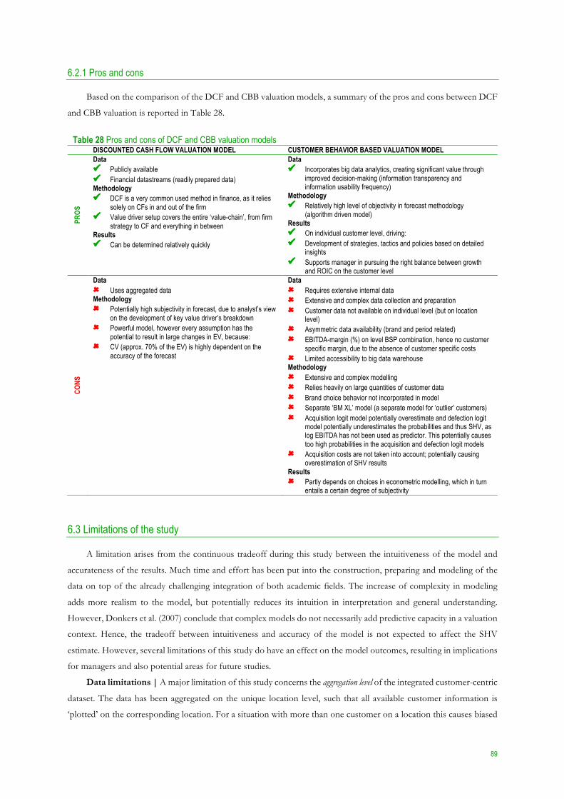
89

6.2.1 Pros and cons

Based on the comparison of the DCF and CBB valuation models, a summary of the pros and cons between DCF

and CBB valuation is reported in Table 28.

Table 28 Pros and cons of DCF and CBB valuation models DISCOUNTED CASH FLOW VALUATION MODEL CUSTOMER BEHAVIOR BASED VALUATION MODEL

PROS

Data ü Publicly available ü Financial datastreams (readily prepared data) Methodology ü DCF is a very common used method in finance, as it relies

solely on CFs in and out of the firm ü Value driver setup covers the entire ‘value-chain’, from firm

strategy to CF and everything in between Results ü Can be determined relatively quickly

Data ü Incorporates big data analytics, creating significant value through

improved decision-making (information transparency and information usability frequency)

Methodology ü Relatively high level of objectivity in forecast methodology

(algorithm driven model) Results ü On individual customer level, driving: ü Development of strategies, tactics and policies based on detailed

insights ü Supports manager in pursuing the right balance between growth

and ROIC on the customer level

CONS

Data û Uses aggregated data Methodology û Potentially high subjectivity in forecast, due to analyst’s view

on the development of key value driver’s breakdown û Powerful model, however every assumption has the

potential to result in large changes in EV, because: û CV (approx. 70% of the EV) is highly dependent on the

accuracy of the forecast

Data û Requires extensive internal data û Extensive and complex data collection and preparation û Customer data not available on individual level (but on location

level) û Asymmetric data availability (brand and period related) û EBITDA-margin (%) on level BSP combination, hence no customer

specific margin, due to the absence of customer specific costs û Limited accessibility to big data warehouse Methodology û Extensive and complex modelling û Relies heavily on large quantities of customer data û Brand choice behavior not incorporated in model û Separate ‘BM XL’ model (a separate model for ‘outlier’ customers) û Acquisition logit model potentially overestimate and defection logit

model potentially underestimates the probabilities and thus SHV, as log EBITDA has not been used as predictor. This potentially causes too high probabilities in the acquisition and defection logit models

û Acquisition costs are not taken into account; potentially causing overestimation of SHV results

Results û Partly depends on choices in econometric modelling, which in turn

entails a certain degree of subjectivity

6.3 Limitations of the study

A limitation arises from the continuous tradeoff during this study between the intuitiveness of the model and

accurateness of the results. Much time and effort has been put into the construction, preparing and modeling of the

data on top of the already challenging integration of both academic fields. The increase of complexity in modeling

adds more realism to the model, but potentially reduces its intuition in interpretation and general understanding.

However, Donkers et al. (2007) conclude that complex models do not necessarily add predictive capacity in a valuation

context. Hence, the tradeoff between intuitiveness and accuracy of the model is not expected to affect the SHV

estimate. However, several limitations of this study do have an effect on the model outcomes, resulting in implications

for managers and also potential areas for future studies.

Data limitations | A major limitation of this study concerns the aggregation level of the integrated customer-centric

dataset. The data has been aggregated on the unique location level, such that all available customer information is

‘plotted’ on the corresponding location. For a situation with more than one customer on a location this causes biased

90

estimates in the first place. The following example will illustrate the most extreme scenario possible causing bias in

estimation: “customer ‘A’ defected from the firm, where customer ‘B’ was newly acquired by the firm during the same

period.” The model assumes individual customers, such that in terms of ‘dummies’ the same customer has a ‘1’ for

defection and a ‘1’ for acquisition. The effect of bias in the estimation due to the location aggregated data is not

obvious, such that it potentially can underestimate or overestimate SHV.

In addition, asymmetry in data availability46 potentially causes biased estimates as well. However, due to the ‘extra

data layer’ resulting from the extracted customer behavior value driver the impact has been reduced to a minimum.

Obviously, missing data is not beneficial for a model heavily relying on large quantities of data. The effect of bias in

the estimation due to asymmetrical data availability is not obvious, such that it potentially can underestimate or

overestimate SHV.

Then, the absence of customer specific margin, potentially causes biased estimates as well. A customer’s total EBITDA

contribution is the sum of its revenues per BSP combination times the firm level EBITDA-margin (%) for each of the

BSP combinations. The effect of bias in the estimation due to the use of ‘average margins (%)’ is not obvious, such

that it potentially can underestimate or overestimate SHV. However, in empirical marketing studies average absolute

margins are typically used, such that the more specific setup in this study is preferred.

Finally, due to limited accessibility into the data warehouse, the concept of big data analytics is not used to its full

potential. In essence the integrated customer-centric dataset contains solely product ownership information, using just

a fraction of the enormous size of data available to the firm’s analysts. This leaves a wide variety of other data sources

like ‘web-data’ ‘mobile data,’ ‘customer-service data’ and many more, unused. Normally, more data leads to more and

potentially better predictors, resulting in better estimates. It is however not possible to determine whether not

incorporating these data has caused underestimation or overestimation of SHV.

Methodological limitations | Another quite major limitation of this study is the fact that the effect of brands has

not been incorporated as part of customer behavior and thus profitability. Incorporating customer brand choice

behavior in the model would have increased the number of behavior logit models from 18 to 72. It is estimated that

this would have increased the computed customer behavior probabilities from 2 to 18 billion, driving the current

150GB of data up to 1TB. This is simply impossible with a ‘home configuration.’ In addition, it is also impossible to

determine whether not incorporating customer brand choice behavior has caused underestimation or overestimation

of SHV.

Then, another important limitation is the absence of an ‘outlier model.’ Certain BM customers have been eliminated

from the analysis, as they were marked as outliers. However, these ‘BM XL’ customers represent more than half of

total BM EBITDA (2014). Therefore, these customers require special attention in analysis and forecasting. This implies

that an additional configuration of 4 profit regression models and 9 behavior logit models was needed for these BM

XL customers. However, due to limited time and computing power this has not been executed. This limitation

potentially underestimates SHV.

Next, another major limitation is the absence of EBITDA contribution (or actually log EBITDA) from the

previous period as a predictor in the acquisition logit model and defection logit model. Adding this predictor for model

estimation would not have been an issue. However, for computing all the equations and producing the probability

output it would have been troubling. An example is used to clarify the ‘strangled equation’ situation:

46 The development of the integrated customer-centric dataset was a first time attempt. Therefore, revenues from value added services (VAS)

have by mistake not been separated from total revenues. As a consequence, valuable insights on customer behavior are ‘lost.’

91

§ The #$%&')$*+#",-. uses among other predictors log-, 234567",-8 as input for computing the

9(;<=>&?&'&$@",-.)

§ Then, 9(;<=>&?&'&$@",-.) is used as input among other predictors in BC$D&')$*+#",-.to compute

log-, 234567",-.

§ Next, log-, 234567",-. is used as input among other predictors in #$%&')$*+#",-E that uses

among other predictors log-, 234567",-. as input for computing the 9(;<=>&?&'&$@",-E)

This process should have been applied for 4 profit regression models 9 behavior logit models for 2 segments,

obviously complicating the computations. The limitation arises from the fact that the acquisition models may produce

probabilities for already acquired customers, hence potentially causing to overestimate SHV. For the defection model

the opposite situation applies, thereby potentially underestimating SHV.

In addition, acquisition costs have not been taken into account in the valuation of acquired customers. And newly

acquired customers are often not yet profitable due to these costs, therefore a firm need to develop its new customers

(Li et al. 2011). Thus, not incorporating acquisition costs causes potentially overestimation of SHV.

Finally, in the forecast of the behavior logit and profit regression models relationship age is a static predictor, where

dynamic is preferred. Or in other words, in case a customer stays with the firm its relationship age for the next period

should have been C+#;'&$@?ℎ&B;%+GH- = (C+#;'&$@?ℎ&B;%+G + 1 C+';&@+*GH- . At first this seems simple to

have this incorporated in the model. However, the complexity of forecasting four periods ahead, given the extensive

number of forecast equations and slow performance of software and hardware, turning this predictor from static into

a dynamic would have come with increased complexity and delay. In addition, due to dataset structure the maximum

relationship age of a customer’s entire portfolio is chosen to serve as input for the prediction. In theory a customer

may retain with the firm, but may churn on its longest relationship product, such that its relationship age plus one

overestimates its relationship age. However, it is more likely a customer is retained on its longest relationship product.

Thus, a static relationship age in forecasting causes potentially underestimation of SHV.

Limitation on results | Limitations on the result arise initially from the fact that the dataset is aggregated on the

unique location level and not on the unique customer level. Interesting insights arise for instance from a customer ranking

based on value, which is obviously less accurate due to the data limitation. However, ranking customers is out of the

scope of this study.

A more complicated matter and potentially a limitation, is the choices made in econometric modelling which in turn

entails a certain degree of subjectivity into the model and thus the results. Moreover, it is not known how different

ways of econometric modeling would affect SHV. However, Donkers et al. (2007) conclude that more complex models

do not necessarily deliver better outcomes and thus valuations aren’t necessarily more accurate.

6.4 Managerial implications

The use of big data, developed methodology, results and conclusions of this study have implications for both

senior executives and managers.

Managerial implication of current data challenges | It is vital that senior executives and managers put priority

on the availability and accessibility of all customer related data, in order to improve the application of big data analytics. A

deeper integration of existing and new big data sources combined with new advanced analytics tools and technology

is crucial for a continuous development of new big data analytics applications, ultimately enhancing SHV.

92

Managerial implication of margin methodologies | Academics have left the topic of margins and costs

underexposed. In modeling customer margins at least three aspects of costs need to be considered: marketing,

administrative and CAPEX. Basically there are two approaches possible in modeling customer specific margins.

The first approach is based on accounting systems. In order to track a customer’s marketing costs, a customer-based

accounting system47 is needed. First, acquisition and retention costs need to be separated. Then, marketing overhead

costs need to be allocated to either one of them. Next, it is important to see whether administrative and other operating

costs are either fixed or semi-fixed. Finally, an activity-based costs accounting system48 supports in forecasting

CAPEX.

The second approach is based on big data analytics but has a more experimental nature. The simple idea behind this

approach is that big data contains such a large amount of information on a single customer that based on this

information costs can be allocated. For instance, let’s take the annual costs of a customer service call center. Assuming

that in big data each phone call and length are registered for each customer, then costs can be easily allocated to the

individual customer. As the customers annual share of total minutes’ times the call center costs, results in the customer

specific costs.

6.4.1 Directions for future studies

ROIC on the individual customer level | Valuation theory states that improvements in ROIC and growth and

the right balance between them drives CFs. Then, CFs discounted at the COC is what ultimately drives SHV. A forward

looking ROIC and growth rate are therefore very insightful parameters. With existing models, it is straightforward to

determine future growth of an individual customer. However, estimating the future ROIC of an individual customer

is more complicated. First of all, because of the already discussed missing ‘customer specific costs’ component. But

mainly because the optimization of investment–return relation is not straightforward on the individual customer level.

The estimated future ROIC of an individual customer would certainly bring valuable managerial insights. Thus, the

challenge for future studies is to investigate the individual customer investment optimization.

Modeling CV on the individual customer level | The CV across all models and scenarios represents 71–75%

of the EV. As the CV has a tremendous impact on the valuation it is important to understand the impact on firm value

when CV is determined on the individual customer level. It logically follows that the derivation of the CV on the

individual customer level potentially contributes to even more accurate firm valuations. A CV estimation on the

individual customer level implies the estimation of a customer specific growth rate and ROIC, as being key input

variables in the key value driver formula. In addition, in the forecast of both DCF and CBB valuation models there is

accounted for idiosyncratic risk. Both models account also for systematic risk by discounting CFs at the WACC.

However, in case of the CV methodology the idiosyncratic risk is more or less incorporated in the assumption on the

growth rate and ROIC. Therefore, a customer specific CV estimation is more capable of accounting for different levels

of idiosyncratic risk. Thus, the challenge for future studies is to investigate impact of the CV methodology on the

individual customer level on total firm value.

47 Marn & Rosiello (1992): “A customer-based accounting system can support in managing prices and results in superior profitability.” 48 Bowman & Narayandas (2004) and Niraj et al. (2001): “An activity-based costs accounting system supports in obtaining better cost estimates

for determining CLV.”

93

6.5 System requirements

The serious shortcoming of software and hardware has been mentioned throughout this report several times.

However, this matter has such great impact on the design of this study that it requires full attention by this paragraph.

Big data analytics consists of: large quantities of data, extensive data preparation, extensive analysis, complex modeling,

heavy duty model estimation and computation. This requires massive computing power and software capabilities.

Especially model estimation is a demanding process in terms of computing power. Therefore, it is highly recommended

to use server capacity for at least model estimation, but preferably also for preparing data and calculating equations.

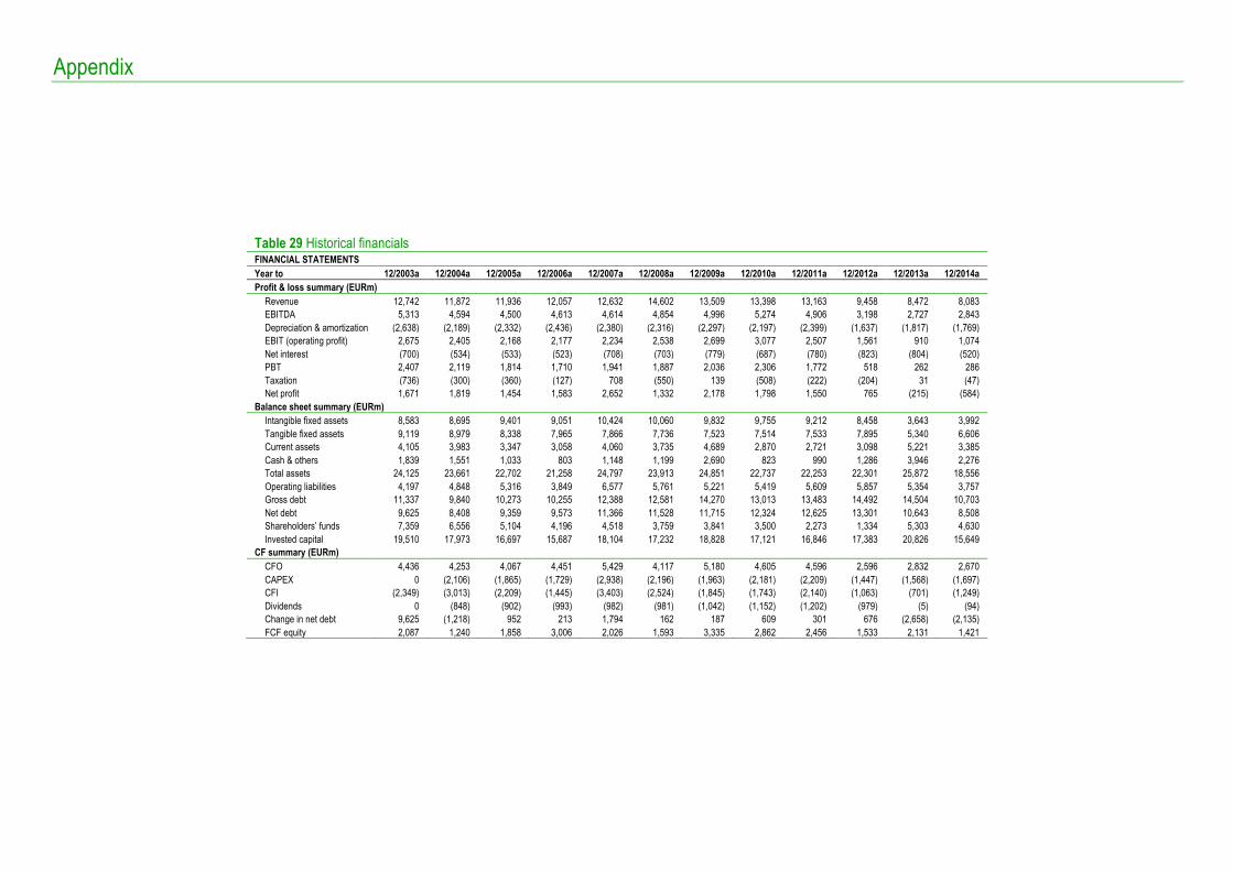
Appendix

Table 29 Historical financials FINANCIAL STATEMENTS Year to 12/2003a 12/2004a 12/2005a 12/2006a 12/2007a 12/2008a 12/2009a 12/2010a 12/2011a 12/2012a 12/2013a 12/2014a Profit & loss summary (EURm)

Revenue 12,742 11,872 11,936 12,057 12,632 14,602 13,509 13,398 13,163 9,458 8,472 8,083 EBITDA 5,313 4,594 4,500 4,613 4,614 4,854 4,996 5,274 4,906 3,198 2,727 2,843 Depreciation & amortization (2,638) (2,189) (2,332) (2,436) (2,380) (2,316) (2,297) (2,197) (2,399) (1,637) (1,817) (1,769) EBIT (operating profit) 2,675 2,405 2,168 2,177 2,234 2,538 2,699 3,077 2,507 1,561 910 1,074 Net interest (700) (534) (533) (523) (708) (703) (779) (687) (780) (823) (804) (520) PBT 2,407 2,119 1,814 1,710 1,941 1,887 2,036 2,306 1,772 518 262 286 Taxation (736) (300) (360) (127) 708 (550) 139 (508) (222) (204) 31 (47) Net profit 1,671 1,819 1,454 1,583 2,652 1,332 2,178 1,798 1,550 765 (215) (584)

Balance sheet summary (EURm) Intangible fixed assets 8,583 8,695 9,401 9,051 10,424 10,060 9,832 9,755 9,212 8,458 3,643 3,992 Tangible fixed assets 9,119 8,979 8,338 7,965 7,866 7,736 7,523 7,514 7,533 7,895 5,340 6,606 Current assets 4,105 3,983 3,347 3,058 4,060 3,735 4,689 2,870 2,721 3,098 5,221 3,385 Cash & others 1,839 1,551 1,033 803 1,148 1,199 2,690 823 990 1,286 3,946 2,276 Total assets 24,125 23,661 22,702 21,258 24,797 23,913 24,851 22,737 22,253 22,301 25,872 18,556 Operating liabilities 4,197 4,848 5,316 3,849 6,577 5,761 5,221 5,419 5,609 5,857 5,354 3,757 Gross debt 11,337 9,840 10,273 10,255 12,388 12,581 14,270 13,013 13,483 14,492 14,504 10,703 Net debt 9,625 8,408 9,359 9,573 11,366 11,528 11,715 12,324 12,625 13,301 10,643 8,508 Shareholders’ funds 7,359 6,556 5,104 4,196 4,518 3,759 3,841 3,500 2,273 1,334 5,303 4,630 Invested capital 19,510 17,973 16,697 15,687 18,104 17,232 18,828 17,121 16,846 17,383 20,826 15,649

CF summary (EURm) CFO 4,436 4,253 4,067 4,451 5,429 4,117 5,180 4,605 4,596 2,596 2,832 2,670 CAPEX 0 (2,106) (1,865) (1,729) (2,938) (2,196) (1,963) (2,181) (2,209) (1,447) (1,568) (1,697) CFI (2,349) (3,013) (2,209) (1,445) (3,403) (2,524) (1,845) (1,743) (2,140) (1,063) (701) (1,249) Dividends 0 (848) (902) (993) (982) (981) (1,042) (1,152) (1,202) (979) (5) (94) Change in net debt 9,625 (1,218) 952 213 1,794 162 187 609 301 676 (2,658) (2,135) FCF equity 2,087 1,240 1,858 3,006 2,026 1,593 3,335 2,862 2,456 1,533 2,131 1,421

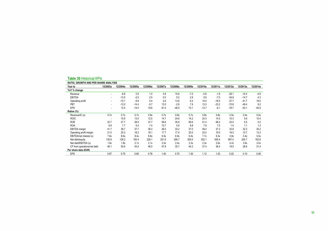
95

Table 30 Historical KPIs RATIO, GROWTH AND PER SHARE ANALYSIS Year to 12/2003a 12/2004a 12/2005a 12/2006a 12/2007a 12/2008a 12/2009a 12/2010a 12/2011a 12/2012a 12/2013a 12/2014a YoY % change

Revenue - -6.8 0.5 1.0 4.8 15.6 -7.5 -0.8 -1.8 -28.1 -10.4 -4.6 EBITDA - -13.5 -2.0 2.5 0.0 5.2 2.9 5.6 -7.0 -34.8 -14.7 4.3 Operating profit - -10.1 -9.9 0.4 2.6 13.6 6.3 14.0 -18.5 -37.7 -41.7 18.0 PBT - -12.0 -14.4 -5.7 13.5 -2.8 7.9 13.3 -23.2 -70.8 -49.4 9.2 EPS - 12.5 -14.0 19.6 81.0 -46.5 73.1 -13.7 -8.1 -78.7 -53.1 -45.5

Ratios (%) Revenue/IC (x) 0.7x 0.7x 0.7x 0.8x 0.7x 0.8x 0.7x 0.8x 0.8x 0.5x 0.4x 0.5x ROIC - 10.9 13.0 12.5 14.7 24.6 14.2 24.3 14.5 10.3 5.6 15.4 ROE 22.7 27.7 28.5 37.7 58.6 35.6 56.6 51.4 68.2 23.5 5.5 5.2 ROA 6.9 7.7 6.4 7.4 10.7 5.6 8.8 7.9 7.0 1.4 1.1 1.3 EBITDA margin 41.7 38.7 37.7 38.3 36.5 33.2 37.0 39.4 37.3 33.8 32.2 35.2 Operating profit margin 21.0 20.3 18.2 18.1 17.7 17.4 20.0 23.0 19.0 16.5 10.7 13.3 EBITDA/net interest (x) 7.6x 8.6x 8.4x 8.8x 6.5x 6.9x 6.4x 7.7x 6.3x 3.9x 3.4x 5.5x Net debt/equity 130.8 128.2 183.4 228.1 251.6 306.7 305.0 352.1 555.4 997.0 200.7 183.8 Net debt/EBITDA (x) 1.8x 1.8x 2.1x 2.1x 2.5x 2.4x 2.3x 2.3x 2.6x 4.2x 3.9x 3.0x CF from operations/net debt 46.1 50.6 43.4 46.5 47.8 35.7 44.2 37.4 36.4 19.5 26.6 31.4

Per share data (EUR) EPS 0.67 0.75 0.65 0.78 1.40 0.75 1.30 1.12 1.03 0.22 0.10 0.06

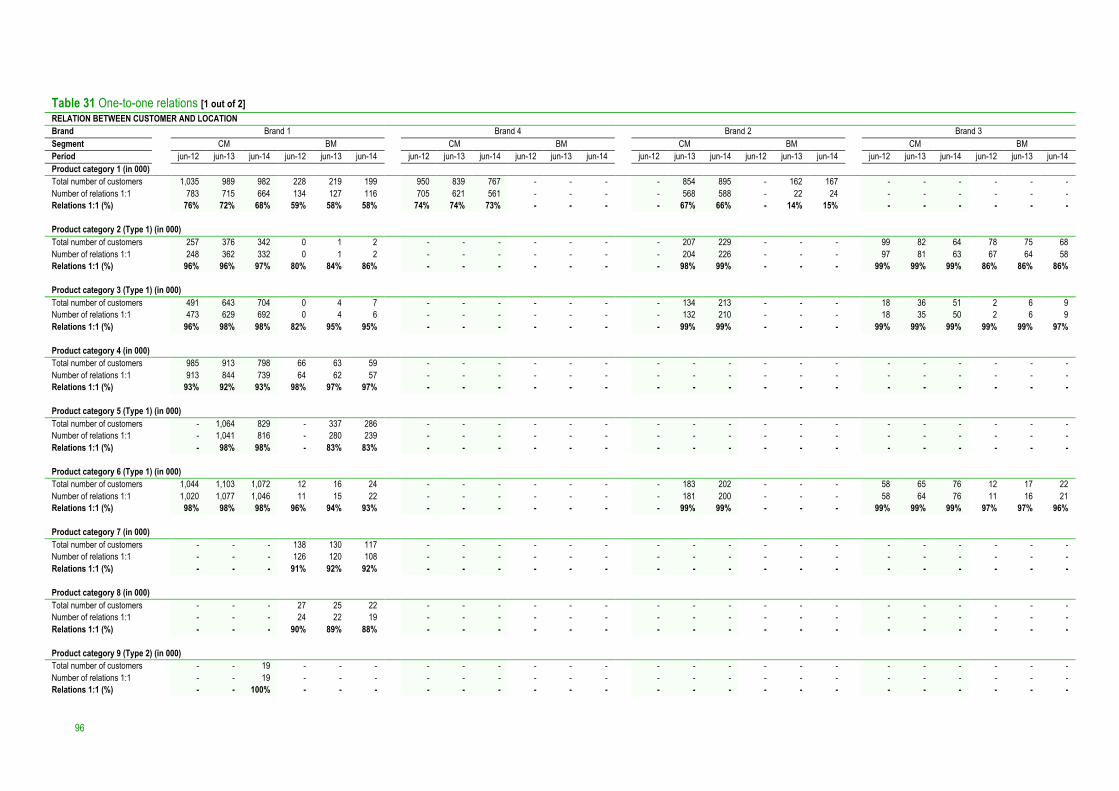
96

Table 31 One-to-one relations [1 out of 2] RELATION BETWEEN CUSTOMER AND LOCATION Brand Brand 1 Brand 4 Brand 2 Brand 3 Segment CM BM CM BM CM BM CM BM Period jun-12 jun-13 jun-14 jun-12 jun-13 jun-14 jun-12 jun-13 jun-14 jun-12 jun-13 jun-14 jun-12 jun-13 jun-14 jun-12 jun-13 jun-14 jun-12 jun-13 jun-14 jun-12 jun-13 jun-14 Product category 1 (in 000) Total number of customers 1,035 989 982 228 219 199 950 839 767 - - - - 854 895 - 162 167 - - - - - - Number of relations 1:1 783 715 664 134 127 116 705 621 561 - - - - 568 588 - 22 24 - - - - - - Relations 1:1 (%) 76% 72% 68% 59% 58% 58% 74% 74% 73% - - - - 67% 66% - 14% 15% - - - - - - Product category 2 (Type 1) (in 000) Total number of customers 257 376 342 0 1 2 - - - - - - - 207 229 - - - 99 82 64 78 75 68 Number of relations 1:1 248 362 332 0 1 2 - - - - - - - 204 226 - - - 97 81 63 67 64 58 Relations 1:1 (%) 96% 96% 97% 80% 84% 86% - - - - - - - 98% 99% - - - 99% 99% 99% 86% 86% 86% Product category 3 (Type 1) (in 000) Total number of customers 491 643 704 0 4 7 - - - - - - - 134 213 - - - 18 36 51 2 6 9 Number of relations 1:1 473 629 692 0 4 6 - - - - - - - 132 210 - - - 18 35 50 2 6 9 Relations 1:1 (%) 96% 98% 98% 82% 95% 95% - - - - - - - 99% 99% - - - 99% 99% 99% 99% 99% 97% Product category 4 (in 000) Total number of customers 985 913 798 66 63 59 - - - - - - - - - - - - - - - - - - Number of relations 1:1 913 844 739 64 62 57 - - - - - - - - - - - - - - - - - - Relations 1:1 (%) 93% 92% 93% 98% 97% 97% - - - - - - - - - - - - - - - - - - Product category 5 (Type 1) (in 000) Total number of customers - 1,064 829 - 337 286 - - - - - - - - - - - - - - - - - - Number of relations 1:1 - 1,041 816 - 280 239 - - - - - - - - - - - - - - - - - - Relations 1:1 (%) - 98% 98% - 83% 83% - - - - - - - - - - - - - - - - - - Product category 6 (Type 1) (in 000) Total number of customers 1,044 1,103 1,072 12 16 24 - - - - - - - 183 202 - - - 58 65 76 12 17 22 Number of relations 1:1 1,020 1,077 1,046 11 15 22 - - - - - - - 181 200 - - - 58 64 76 11 16 21 Relations 1:1 (%) 98% 98% 98% 96% 94% 93% - - - - - - - 99% 99% - - - 99% 99% 99% 97% 97% 96% Product category 7 (in 000) Total number of customers - - - 138 130 117 - - - - - - - - - - - - - - - - - - Number of relations 1:1 - - - 126 120 108 - - - - - - - - - - - - - - - - - - Relations 1:1 (%) - - - 91% 92% 92% - - - - - - - - - - - - - - - - - - Product category 8 (in 000) Total number of customers - - - 27 25 22 - - - - - - - - - - - - - - - - - - Number of relations 1:1 - - - 24 22 19 - - - - - - - - - - - - - - - - - - Relations 1:1 (%) - - - 90% 89% 88% - - - - - - - - - - - - - - - - - - Product category 9 (Type 2) (in 000) Total number of customers - - 19 - - - - - - - - - - - - - - - - - - - - - Number of relations 1:1 - - 19 - - - - - - - - - - - - - - - - - - - - - Relations 1:1 (%) - - 100% - - - - - - - - - - - - - - - - - - - - -

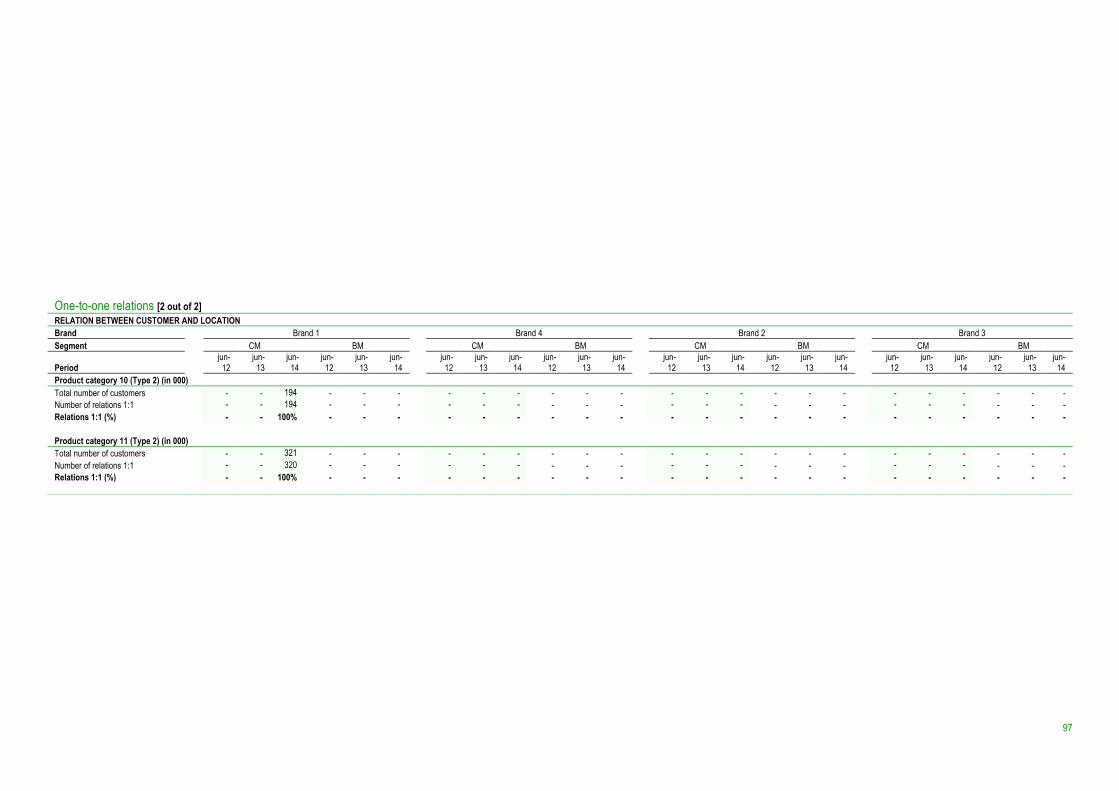
97

One-to-one relations [2 out of 2] RELATION BETWEEN CUSTOMER AND LOCATION Brand Brand 1 Brand 4 Brand 2 Brand 3 Segment CM BM CM BM CM BM CM BM

Period jun-

12 jun-

13 jun-

14 jun-

12 jun-

13 jun-

14 jun-

12 jun-

13 jun-

14 jun-

12 jun-

13 jun-

14 jun-

12 jun-

13 jun-

14 jun-

12 jun-

13 jun-

14 jun-

12 jun-

13 jun-

14 jun-

12 jun-

13 jun-

14 Product category 10 (Type 2) (in 000) Total number of customers - - 194 - - - - - - - - - - - - - - - - - - - - - Number of relations 1:1 - - 194 - - - - - - - - - - - - - - - - - - - - - Relations 1:1 (%) - - 100% - - - - - - - - - - - - - - - - - - - - - Product category 11 (Type 2) (in 000) Total number of customers - - 321 - - - - - - - - - - - - - - - - - - - - - Number of relations 1:1 - - 320 - - - - - - - - - - - - - - - - - - - - - Relations 1:1 (%) - - 100% - - - - - - - - - - - - - - - - - - - - -

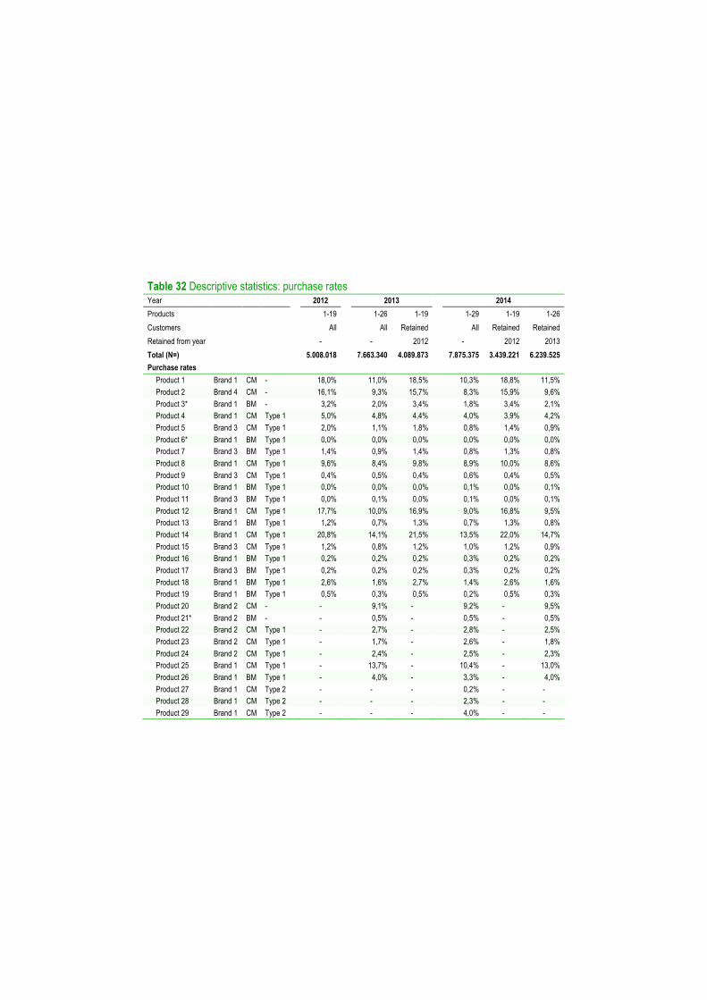
Table 32 Descriptive statistics: purchase rates Year 2012 2013 2014

Products 1-19 1-26 1-19 1-29 1-19 1-26

Customers All All Retained All Retained Retained

Retained from year - - 2012 - 2012 2013

Total (N=) 5.008.018 7.663.340 4.089.873 7.875.375 3.439.221 6.239.525 Purchase rates

Product 1 Brand 1 CM - 18,0% 11,0% 18,5% 10,3% 18,8% 11,5% Product 2 Brand 4 CM - 16,1% 9,3% 15,7% 8,3% 15,9% 9,6% Product 3* Brand 1 BM - 3,2% 2,0% 3,4% 1,8% 3,4% 2,1% Product 4 Brand 1 CM Type 1 5,0% 4,8% 4,4% 4,0% 3,9% 4,2% Product 5 Brand 3 CM Type 1 2,0% 1,1% 1,8% 0,8% 1,4% 0,9% Product 6* Brand 1 BM Type 1 0,0% 0,0% 0,0% 0,0% 0,0% 0,0% Product 7 Brand 3 BM Type 1 1,4% 0,9% 1,4% 0,8% 1,3% 0,8% Product 8 Brand 1 CM Type 1 9,6% 8,4% 9,8% 8,9% 10,0% 8,6% Product 9 Brand 3 CM Type 1 0,4% 0,5% 0,4% 0,6% 0,4% 0,5% Product 10 Brand 1 BM Type 1 0,0% 0,0% 0,0% 0,1% 0,0% 0,1% Product 11 Brand 3 BM Type 1 0,0% 0,1% 0,0% 0,1% 0,0% 0,1% Product 12 Brand 1 CM Type 1 17,7% 10,0% 16,9% 9,0% 16,8% 9,5% Product 13 Brand 1 BM Type 1 1,2% 0,7% 1,3% 0,7% 1,3% 0,8% Product 14 Brand 1 CM Type 1 20,8% 14,1% 21,5% 13,5% 22,0% 14,7% Product 15 Brand 3 CM Type 1 1,2% 0,8% 1,2% 1,0% 1,2% 0,9% Product 16 Brand 1 BM Type 1 0,2% 0,2% 0,2% 0,3% 0,2% 0,2% Product 17 Brand 3 BM Type 1 0,2% 0,2% 0,2% 0,3% 0,2% 0,2% Product 18 Brand 1 BM Type 1 2,6% 1,6% 2,7% 1,4% 2,6% 1,6% Product 19 Brand 1 BM Type 1 0,5% 0,3% 0,5% 0,2% 0,5% 0,3% Product 20 Brand 2 CM - - 9,1% - 9,2% - 9,5% Product 21* Brand 2 BM - - 0,5% - 0,5% - 0,5% Product 22 Brand 2 CM Type 1 - 2,7% - 2,8% - 2,5% Product 23 Brand 2 CM Type 1 - 1,7% - 2,6% - 1,8% Product 24 Brand 2 CM Type 1 - 2,4% - 2,5% - 2,3% Product 25 Brand 1 CM Type 1 - 13,7% - 10,4% - 13,0% Product 26 Brand 1 BM Type 1 - 4,0% - 3,3% - 4,0% Product 27 Brand 1 CM Type 2 - - - 0,2% - - Product 28 Brand 1 CM Type 2 - - - 2,3% - - Product 29 Brand 1 CM Type 2 - - - 4,0% - -

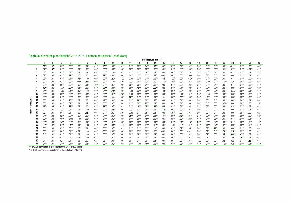
Table 33 Ownership correlations 2013-2014 (Pearson correlation r-coefficient) Product type jun-14 1 2 3 4 5 6 7 8 9 10 11 12 13 14 15 16 17 18 19 20 21 22 23 24 25 26

Prod

uct t

ype

jun-

13

1 .86** .07** .03** .06** .02** .01** .01** .13** .01** .01** .01** .08** .04** .15** .02** .02** .01** .02** .00** .01** .01** .00** -.01** -.01** .03** .04** 2 .07** .87** .01** .03** .01** .00** .00** .06** .01** .00** .00** .06** .02** .06** .01** .01** .00** .00** .00** .03** .00** .01** .02** .01** -.01** .01** 3 .03** .01** .87** .02** .01** .02** .09** .00** .00 .04** .02** .02** .09** .01** .00** .06** .03** .18** .14** -.01** .07** .00** -.01** -.01** .02** .24** 4 .07** .04** .02** .77** .00** .00** .00** .29** -.01** .00** .00** .12** .02** .18** -.01** .00** .00** .00* .00** .02** .01** .00** .00** -.01** .01** .01** 5 .03** .01** .01** -.01** .76** .00 .00** -.02** .20** .00 0.00 .02** .01** -.02** .14** .00* .00** 0.00 .00** .01** .00** -.01** -.01** -.01** .09** .03** 6 .00** .00** .02** .00** 0.00 .59** .00** .00** .00 .19** .00* .00** .02** .00** .00 .15** .00** .01** .00** 0.00 .01** .00 .00* .00** .00** .02** 7 .01** .00** .09** .00** .00** .01** .79** -.01** .00** .00** .09** .00** .04** -.02** .00** .01** .09** .05** .07** -.01** .04** .00** -.01** -.01** .02** .14** 8 .13** .06** .00* .28** -.01** .00** -.01** .79** -.01** .00** .00** .19** .03** .55** -.02** -.01** -.01** -.02** -.01** .03** .00** -.02** .00** -.01** -.05** -.02** 9 .01** .01** .00 -.01** .15** .00* .00** -.01** .71** .00** .00 .03** .00** -.01** .44** .00** .00** .00** .00** .01** .00** .00** 0.00 .00** -.01** -.01**

10 .01** .00** .03** .00** .00** .16** .00** .00** .00** .73** 0.00 .00** .05** -.01** .00** .39** .00* .01** .00** .00 .01** .00** .00** .00** .00** .01** 11 .00** .00** .01** .00** .00** .00** .06** .00** 0.00 .00** .70** .01** .01** -.01** .00* .00** .36** .00** .00** .00* .01** .00** .00** .00** .00** .00** 12 .08** .06** .02** .10** .02** .00** .00** .17** .04** .00** .01** .80** .00** .16** .03** .01** .01** .00** .00** .05** .01** .06** .04** .04** .01** .00** 13 .03** .02** .09** .02** .01** .02** .04** .03** .00** .03** .01** .00** .85** .04** .00** .06** .01** .09** .06** .01** .03** 0.00 .00** .00** .00** .15** 14 .15** .06** .01** .16** -.02** .00** -.02** .56** -.02** -.01** -.01** .18** .05** .84** -.02** -.01** -.01** -.02** -.01** .03** .00** -.03** -.02** -.02** -.07** -.03** 15 .01** .01** .00* -.01** .02** .00* .00** -.02** .46** .00** .00* .03** .00** -.02** .78** .00** .00** -.01** .00** .01** .00** -.01** .00** -.01** -.01** -.01** 16 .02** .01** .04** -.01** .00** .13** .00** -.01** .00** .39** 0.00 .01** .06** -.01** .00** .79** .00** .01** .00** .00** .01** .00** .00** .00** .00** .02** 17 .01** .00** .02** .00** .00** .00** .03** -.01** .00** .00** .36** .01** .01** -.01** .00* .00** .75** .01** .01** .00** .01** .00** .00** .00** .00** .02** 18 .02** .00** .18** 0.00 .00 .02** .05** -.01** .00** .03** .01** .00** .10** -.02** -.01** .05** .02** .84** .13** -.01** .06** -.01** -.01** -.01** .01** .35** 19 .00** .00** .14** .00** .00** .01** .07** -.01** .00** .00** .00** .00** .06** -.01** .00** .01** .01** .14** .87** -.01** .04** .00** -.01** .00** .00** .19** 20 .00** .02** -.01** .01** .01** .00 -.01** .02** .01** .00 .00** .05** .01** .02** .01** .00 .00** -.01** -.01** .83** .02** .07** .09** .08** -.02** -.01** 21 .00** .00** .05** .00** .00** .01** .04** .00** .00** .01** .01** .01** .03** .00* .00** .02** .02** .05** .04** .02** .77** .00** .00** .01** .00** .08** 22 .00** .01** .00** -.01** -.01** .00* .00** -.03** -.01** .00** .00** .05** .00** -.03** -.01** .00** .00** -.01** .00** .07** .01** .73** .25** .02** .03** .01** 23 -.01** .01** -.01** -.01** -.01** .00* -.01** -.02** .00** .00** .00** .05** .00** -.03** -.01** .00** .00** -.01** .00** .08** .00** .24** .66** .42** -.02** -.01** 24 -.01** .01** -.01** -.02** -.01** .00* -.01** -.02** .00** .00** .00** .05** .00** -.03** -.01** .00** .00** -.01** .00** .08** .01** .01** .39** .76** -.02** -.01** 25 .04** -.01** .02** .01** .09** .00** .02** -.03** .01** .00** .00** .01** .00** -.03** .01** .00** .00** .01** .00 -.02** .00** .02** -.02** -.01** .86** -.01** 26 .04** .01** .24** .01** .03** .03** .13** -.02** .00** .03** .01** .00 .16** -.02** .00** .07** .03** .35** .17** -.01** .09** .00 -.02** -.01** -.01** .88**

**: p<0.01 (correlation is significant at the 0.01 level, 2-tailed) *: p<0.05 (correlation is significant at the 0.05 level, 2-tailed)

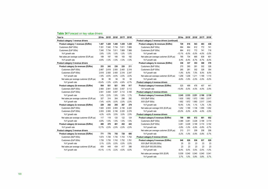
100

Table 34 Forecast on key value drivers Year to 2014a 2015f 2016f 2017f 2018f 2014a 2015f 2016f 2017f 2018f Product category 1 revenue drivers Product category 3 revenue drivers (continued)

Product category 1 revenues (EURm) 1.407 1.429 1.440 1.439 1.439 Product category 3b revenues (EURm) 729 616 543 483 438 Customers (BoP 000s) 7.351 7.540 7.734 7.811 7.889 Customers (BoP 000s) 994 864 812 772 741 Customers (EoP 000s) 7.540 7.734 7.811 7.889 7.968 Customers (EoP 000s) 864 812 772 741 718

YoY growth rate 2,6% 1,0% 1,0% 1,0% 1,0% YoY growth rate -13,1% -6,0% -5,0% -4,0% -3,0%

Net sales per average customer (EUR pa) 189 187 185 183 182 Net sales per average customer (EUR pa) 785 734 685 639 601 YoY growth rate -6,6% -1,0% -1,0% -1,0% -1,0% YoY growth rate 6,4% -6,4% -6,7% -6,7% -6,0%

Product category 2 revenue drivers Product category 3c revenues (EURm) 336 337 353 368 378 Product category 2a revenues (EURm) 253 243 230 220 211 Customers (BoP 000s) 270 265 281 302 328

Customers (BoP 000s) 2.667 2.618 2.500 2.400 2.316 Customers (EoP 000s) 265 281 302 328 354 Customers (EoP 000s) 2.618 2.500 2.400 2.316 2.247 YoY growth rate -1,9% 6,0% 7,5% 8,5% 8,0%

YoY growth rate -1,8% -4,5% -4,0% -3,5% -3,0% Net sales per average customer (EUR pa) 1.256 1.236 1.211 1.169 1.110 Net sales per average customer (EUR pa) 96 95 94 93 93 YoY growth rate -9,6% -1,6% -2,0% -3,5% -5,0%

YoY growth rate -18,4% -1,0% -0,9% -0,8% -0,7% Product category 4 revenue drivers Product category 2b revenues (EURm) 954 931 921 919 917 Product category 4 revenues (EURm) 525 499 476 457 441

Customers (BoP 000s) 2.900 2.941 3.000 3.057 3.112 YoY growth rate -15,9% -5,0% -4,5% -4,0% -3,5%

Customers (EoP 000s) 2.941 3.000 3.057 3.112 3.165 Product category 5 revenue drivers YoY growth rate 1,4% 2,0% 1,9% 1,8% 1,7% Product category 5 revenues (EURm) 2.245 2.333 2.251 2.186 2.136

Net sales per average customer (EUR pa) 327 314 304 298 292 XXX (BoP 000s) 1.635 1.952 1.972 1.993 2.017 YoY growth rate -7,4% -4,0% -3,0% -2,0% -2,0% XXX (EoP 000s) 1.952 1.972 1.993 2.017 2.043

Product category 2c revenues (EURm) 229 242 255 267 279 YoY growth rate 19,4% 1,0% 1,1% 1,2% 1,3%

Customers (BoP 000s) 1.920 2.003 2.083 2.156 2.220 Net sales per average XXX (EUR pa) 1.252 1.189 1.136 1.090 1.052 Customers (EoP 000s) 2.003 2.083 2.156 2.220 2.276 YoY growth rate -23,0% -5,0% -4,5% -4,0% -3,5%

YoY growth rate 4,3% 4,0% 3,5% 3,0% 2,5% Product category 6 revenue drivers Net sales per average customer (EUR pa) 117 119 120 122 124 Product category 6 revenues (EURm) 709 685 672 661 652

YoY growth rate -6,8% 1,5% 1,5% 1,5% 1,5% Customers (BoP 000s) 3.389 3.261 3.228 3.199 3.174 Product category 2d revenues (EURm) 480 470 461 452 443 Customers (EoP 000s) 3.261 3.228 3.199 3.174 3.152

YoY growth rate 12,7% -2,0% -2,0% -2,0% -2,0% YoY growth rate -3,8% -1,0% -0,9% -0,8% -0,7%

Product category 3 revenue drivers Net sales per average customer (EUR pa) 213 211 209 208 206 Product category 3a revenues (EURm) 771 776 755 728 695 YoY growth rate -0,2% -1,0% -0,9% -0,8% -0,7%

Customers (BoP 000s) 1.674 1.726 1.735 1.743 1.752 Product category 9 revenue drivers Customers (EoP 000s) 1.726 1.735 1.743 1.752 1.761 Product category 9 revenues (EURm) 948 926 936 937 929

YoY growth rate 3,1% 0,5% 0,5% 0,5% 0,5% XXX (BoP 000,000,000s) 25 23 23 23 23 Net sales per average customer (EUR pa) 454 449 434 417 396 XXX (EoP 000,000,000s) 23 23 23 23 23

YoY growth rate -15,1% -1,1% -3,2% -4,0% -5,0% YoY growth rate -6,4% 0,0% 0,5% -2,0% -1,0% Net sales per average XXX (EUR) 0,039 0,040 0,040 0,040 0,041

YoY growth rate 3,7% 1,0% 0,9% 0,8% 0,7%

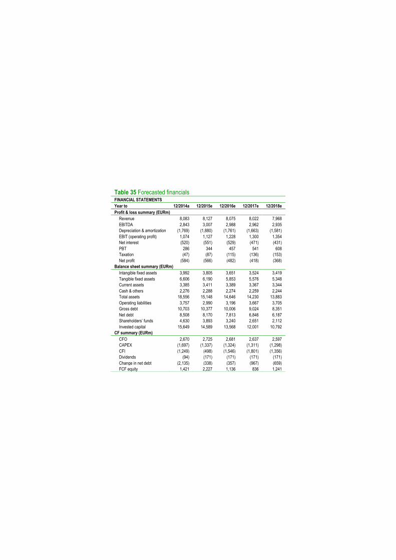
Table 35 Forecasted financials FINANCIAL STATEMENTS Year to 12/2014a 12/2015e 12/2016e 12/2017e 12/2018e Profit & loss summary (EURm)

Revenue 8,083 8,127 8,075 8,022 7,968 EBITDA 2,843 3,007 2,988 2,962 2,935 Depreciation & amortization (1,769) (1,880) (1,761) (1,663) (1,581) EBIT (operating profit) 1,074 1,127 1,228 1,300 1,354 Net interest (520) (551) (529) (471) (431) PBT 286 344 457 541 608 Taxation (47) (87) (115) (136) (153) Net profit (584) (566) (482) (418) (368)

Balance sheet summary (EURm) Intangible fixed assets 3,992 3,805 3,651 3,524 3,419 Tangible fixed assets 6,606 6,190 5,853 5,576 5,348 Current assets 3,385 3,411 3,389 3,367 3,344 Cash & others 2,276 2,288 2,274 2,259 2,244 Total assets 18,556 15,148 14,646 14,230 13,883 Operating liabilities 3,757 2,990 3,196 3,667 3,705 Gross debt 10,703 10,377 10,006 9,024 8,351 Net debt 8,508 8,170 7,813 6,846 6,187 Shareholders’ funds 4,630 3,893 3,240 2,651 2,112 Invested capital 15,649 14,589 13,568 12,001 10,792

CF summary (EURm) CFO 2,670 2,725 2,681 2,637 2,597 CAPEX (1,697) (1,337) (1,324) (1,311) (1,298) CFI (1,249) (498) (1,546) (1,801) (1,356) Dividends (94) (171) (171) (171) (171) Change in net debt (2,135) (338) (357) (967) (659) FCF equity 1,421 2,227 1,136 836 1,241

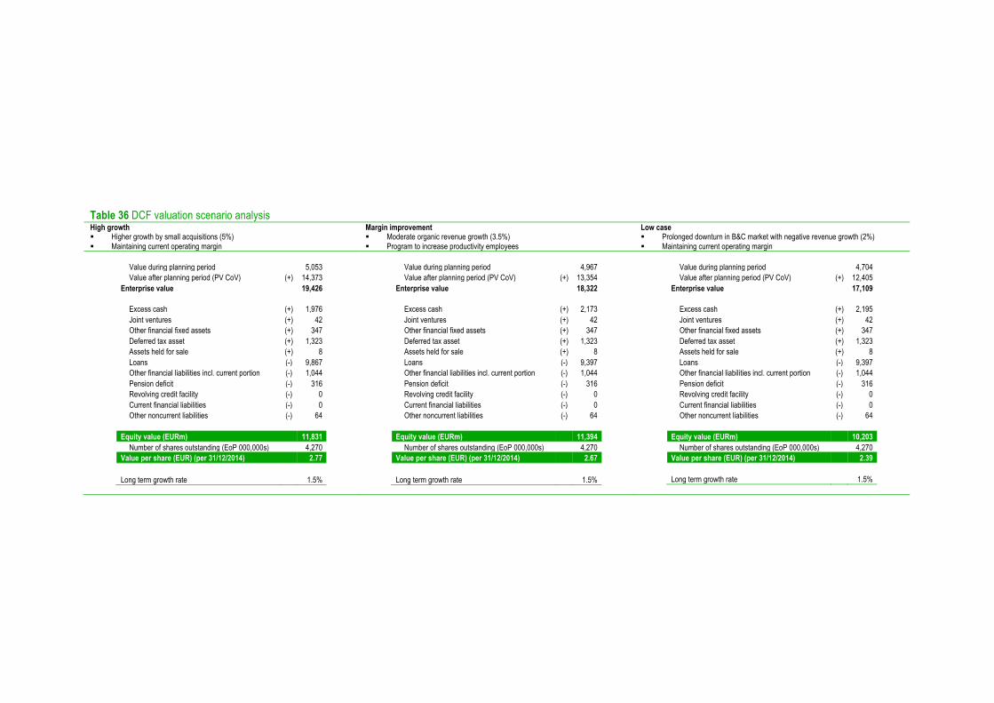
Table 36 DCF valuation scenario analysis High growth Margin improvement Low case § Higher growth by small acquisitions (5%) § Maintaining current operating margin

§ Moderate organic revenue growth (3.5%) § Program to increase productivity employees

§ Prolonged downturn in B&C market with negative revenue growth (2%) § Maintaining current operating margin

Value during planning period 5,053 Value after planning period (PV CoV) (+) 14,373















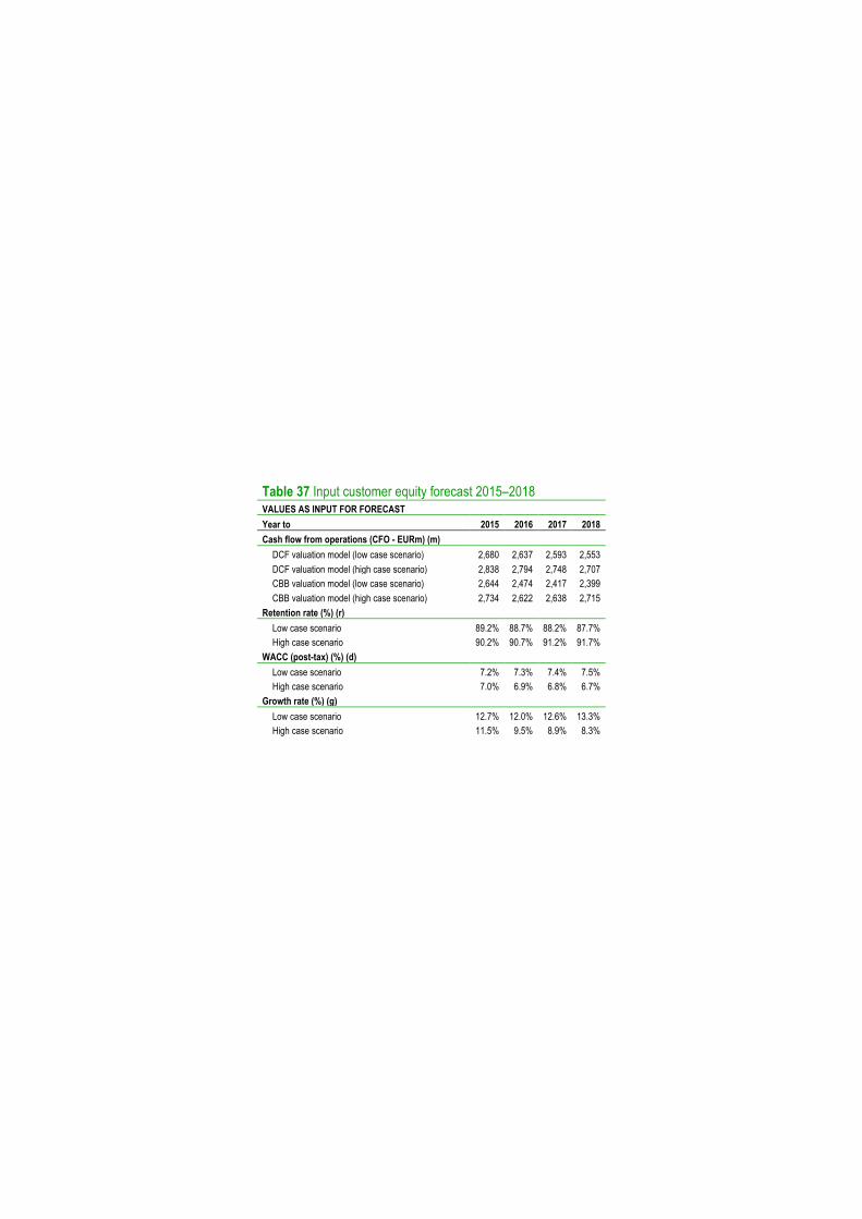
Table 37 Input customer equity forecast 2015–2018 VALUES AS INPUT FOR FORECAST Year to 2015 2016 2017 2018 Cash flow from operations (CFO - EURm) (m)

DCF valuation model (low case scenario) 2,680 2,637 2,593 2,553 DCF valuation model (high case scenario) 2,838 2,794 2,748 2,707 CBB valuation model (low case scenario) 2,644 2,474 2,417 2,399 CBB valuation model (high case scenario) 2,734 2,622 2,638 2,715

Retention rate (%) (r) Low case scenario 89.2% 88.7% 88.2% 87.7% High case scenario 90.2% 90.7% 91.2% 91.7%

WACC (post-tax) (%) (d) Low case scenario 7.2% 7.3% 7.4% 7.5% High case scenario 7.0% 6.9% 6.8% 6.7%

Growth rate (%) (g) Low case scenario 12.7% 12.0% 12.6% 13.3% High case scenario 11.5% 9.5% 8.9% 8.3%

References Aaker, David A. (1996), "Measuring Brand Equity Across Products and Markets," California Management Review, 38

(Spring), 102–120.

Anderson, Eugene W. and Mary W. Sullivan (1993), "The Antecedents and Consequences of Customer Satisfaction

for Firms," Marketing Science, 12 (Spring), 125–143.

Anderson, Erin and Barton Weitz (1989), "Determinants of Continuity in Conventional Industrial Channel Dyads,"

Marketing Science, 8 (Autumn), 310–323.

Bauer, Hans H., Maik Hammerschmidt, and Matthias Braehler (2003), The Customer Lifetime Value Concept and its

Contribution to Corporate Valuation Yearbook of Marketing and Consumer Research, 1 47–67.

Berger, Paul D. and Nada I. Nasr (1998), "Customer Lifetime Value: Marketing Models and Applications," Journal of

Interactive Marketing, 12 (Winter),

Berger, Paul D., Naras Eechambadi, Morris George, Donald R. Lehmann, Ross Rizley, and Rajkumar Venkatesan

(2006), "From Customer Lifetime Value to Shareholder Value Theory, Empirical Evidence, and Issues for

Future Research," Journal of Service Research, 9 (November), 156–167.

Bick, Geoffrey N.C. (2009), "Increasing shareholder value through building Customer and Brand Equity," Journal of

Marketing Management, 25 117–141.

Black, Fischer, M. Jensen, and M. Scholes (1972), “The Capital Asset Pricing Model: Some Empirical Tests,” Studies

in Theory of Capital Markets, ed. M. Jensen, New York: Praeger.

Blattberg, Robergt C. and John Deighton (1996), "Manage Marketing by the Customer Equity Test," Harvard Business

Review, (July), 136–144.

Bolton, Ruth N., P.K. Kannan, and Matthew D. Bramlett (2000), "Implications of Loyalty Program Membership and

Service Experiences for Customer Retention and Value," Journal of the Academy of Marketing Science, 28

(Winter), 95–108.

Bowman, Douglas and Das Narayandas (2004), "Linking Customer Management Effort to Customer Profitability in

Business Markets," Journal of Marketing Research, 61 (November), 433–447.

Bowman, Douglas, John U. Farleyn, and David C. Schmittlein (2000), "Cross-National Empirical Generalization in

Business Services Buying Behavior," Journal of International Business Studies, 31 (December), 667–685.

Brakus Joško J., Bernd H. Schmitt, and Lia Zarantonello (2009), "Brand Experience: What is it? How is it Measured?

Does it Affect Loyalty?" Journal of Marketing, 73 (May), 52–68.

Carhart, Mark (1997), “On Persistence in Mutual Fund Performance,” Journal of Finance, 52 (March), 57–82.

Chaney, Paul K., Timothy M. Devinney, and Russell S. Winer (1991), "The Impact of New Product Introductions on

the Market Valuation of Firms," Journal of Business, 64 (October), 573–610.

Cooil, Bruce, Keiningham, Timothy L., Aksoy, Lerzan, and Hsu, Michael (2007), "A Longitudinal Analysis of

Customer Satisfaction and Share of Wallet: Investigating the Moderating Effect of Customer Characteristics,"

Journal of Marketing, 71 (January), 67–83.

Copeland, Thomas E. (1979), "Liquidity Changes Following Stock Splits," Journal of Finance, 34 (March), 115–141.

Coyles, Stephanie and Timothy C. Gokey (2005), "Customer Retention is not Enough," Journal of Consumer

Marketing, 22 101–105.

Demers, Elizabeth and Baruch Lev (2001), “A Rude Awakening: Internet Shakeout in 2000,” Review of Accounting

Studies, 6 (January), 331–359.

105

Donkers, Bas, Philip Hans Franses, and Peter C. Verhoef (2003), "Selective Sampling for Binary Choice Models,"

Journal of Marketing Research, 60 (November), 492–497.

Donkers, Bas, Peter C. Verhoef, and Martijn G. de Jong (2007), "Modeling CLV: A Test of Competing Models in the

Insurance Industry," Quantitative Marketing and Economics, 5 (June), 163–190.

Doyle, Peter (2000), "Value-Based Marketing," Journal of Strategic Marketing, 8 299–311.

Fader, Peter S., Bruce G.S. Hardie, and Ka Lok Lee (2005), "RFM and CLV: Using Iso-Value Curves for Customer

Base Analysis," Journal of Marketing Research, 42 (November), 415–430.

Fama, Eugene F. (1965), "The Behavior of Stock-Market Prices," Journal of Business, 38 (January), 34–105.

Fama, Eugene F. (1991), "Efficient Capital Markets: II," Journal of Finance, 46 (December), 1575–1617.

Fama, Eugene F. and Kenneth R. French (1992), "The Cross-Section of Expected Stock Returns," Journal of Finance,

47 (June), 427–465.

Fama, Eugene F. and Kenneth R. French (1996), The CAPM is Wanted, Dead or Alive Journal of Finance, 51

(December), 1947–1958.

Graham, J.R., C. Harvey and S. Rajgopal (2005), “The Economic Implications of Corporate Financial Reporting,”

Journal of Accounting and Economics, 40, 3–73.

Gupta, Sunil (2009), "Customer-Based Valuation," Journal of Interactive Marketing, 23 169–178.

Gupta, Sunil and Donald R. Lehmann (2003), "Customers as Assets," Journal of Interactive Marketing, 17 (Winter),

9–24.

Gupta, Sunil and Donald R. Lehmann (2006), "Customer Lifetime Value and Firm Valuation," Journal of Relationship

Marketing, 5 (September), 87–110.

Gupta, Sunil, Donald R. Lehmann, and Jennifer A. Stuart (2004), "Valuing Customers," Journal of Marketing Research,

61 (February), 7–18.

Gupta, Sunil and Valarie Zeithaml (2006), “Customer Metrics and Their Impact on Financial Performance,” Marketing

Science, 25 (6), 718–39.

Gupta, Sunil, Dominique Hanssens, Bruce Hardie, Kahn William, V. Kumar, Nathaniel Lin, Nalini Ravishanker, and

S. Sriram (2006), "Modeling Customer Lifetime Value," Journal of Service Research, 9 (November), 139–155.

Hamada, Robert S. (1972), "The Effect of the Firm's Capital Structure on the Systematic Risk of Common Stocks,"

Journal of Finance, 27 (May), 435–452.

Hauser, John R. and Glen L. Urban (1986), "The Value Priority Hypotheses for Consumer Budget Plans," Journal of

Consumer Research, 12 (March) 446–462.

Hogan, John E., Donald R. Lehmann, Maria Merino, Rajendra K. Srivastava, Jacquelyn S. Thomas, and Peter C.

Verhoef (2002), "Linking Customer Assets to Financial Performance," Journal of Service Research, 5 (August),

26–38.

Hogan, John E., Katherine N. Lemon, and Roland T. Rust (2002), "Customer Equity Management Charting New

Directions for the Future of Marketing," Journal of Service Research, 5 (August), 4–12.

Homburg, Christian, Annette Giering, and Ajay Menon (2003), "Relationship Characteristics as Moderators of the

Satisfaction-Loyalty Link: Findings in a Business-to- Business Context," Journal of Business-to-Business

Marketing, 10 35–62.

Jain, Dipak and Siddhartha S. Singh (2002), "Customer Lifetime Value Research in Marketing: A Review and Future

Directions," Journal of Interactive Marketing, 34–46.

106

Jiang, Bin and Tim Koller (2007), “How to Choose between Growth and ROIC,” McKinsey on Finance, 25 (Autumn),

19–22.

Jones, Thomas O. and W.E. Sasser (1995), "Why Satisfied Customers Defect," Harvard Business Review, 73

(November), 88–99.

Kalwani, Manohar U. and Narakesari Narayandas (1995), “Long-Term Manufacturer-Supplier Relationships: Do They

Pay Off for the Supplier Firm?,” Journal of Marketing, 59 1–16.

Kamakura, Wagner A., Sridhar N. Ramaswami, and Rajendra K. Srivastava, (1991), "Applying Latent Trait Analysis in

the Evaluation of Prospects for Cross-Selling of Financial Services," International Journal of Research in

Marketing 8 (November), 329–349.

Keiningham, Timothy L., Bruce Cooil, Lerzan Aksoy, Tor W. Andreassen, and Jay Weiner (2007), "The Value of

Different Customer Satisfaction and Loyalty Metrics in Predicting Customer Retention, Recommendation, and

Share-of-Wallet," Managing Service Quality, 17 361–384.

Keller, Kevin L. (1993), "Conceptualizing, Measuring, and Managing Customer-Based Brand Equity," Journal of

Marketing, 57 (January), 1–22.

Kim, Byung-Do and Sun-Ok Kim (1999), “Measuring Upselling Potential for Life Insurance Customers," Journal of

Interactive Marketing, 13 2–9.

Kim, Namwoon, Vijay Mahajan, and Rajendra K. Srivastava (1995), “Determining the Going Market Value of a

Business in an Emerging Information Technology Industry: The Case of the Cellular Communication Industry,”

Technological Forecasting and Social Change, 49 257–279.

Knott, Aaron, Andrew Hayes, and Scott A. Neslin (2002), "Next�Product�to�Buy Models for Cross�Selling

Applications," Journal of Interactive Marketing, 16 (Summer), 59�75.

Kumar V. and Denish Shah (2009), "Expanding the Role of Marketing: From Customer Equity to Market

Capitalization," Journal of Marketing, 73 (November), 119–136.

Lemon, Katherine N., Roland T. Rust, and Valarie A. Zeithaml (2001), "What Drives Customer Equity," Marketing

Management, 10 (Spring), 20–25.

Leone, Robert P., Vithala R. Rao, Kevin L. Keller, Anita M. Luo, Leigh McAlister, and Rajendra Srivastava (2006),

"Linking Brand Equity to Customer Equity," Journal of Service Research, 9 (November), 125–138.

Lev, Baruch (2004), "Sharpening the Intangibles Edge," Harvard Business Review, (June), 109–116.

Li, Shibo, Baohong Sun, and Ronald T. Wilcox (2005), "Cross-Selling Sequentially Ordered Products: An Application

to Consumer Banking Services," Journal of Marketing Research, 62 (May), 233–239,

Libai, Barak, Eitan Muller, and Renana Peres (2009), "The Diffusion of Services," Journal of Marketing Research, 66

(April), 163–175.

Malthouse, Edward C. and Robert C. Blattberg (2005), "Can We Predict Customer Lifetime Value?," Journal of

Interactive Marketing, 19 (Winter), 2–16.

Marn, Michael V. and Robert L. Rosiello (1992), "Managing Price, Gaining Profit," Harvard Business Review,

(September), 84–94.

McAlister, Leigh and E. Pessemier (1982), “Variety Seeking Behavior: An Interdisciplinary Review,"" Journal of

Consumer Research 9 (December), 311–322."

McAlister, Leigh, Raji Srinivasan, and Min Chung Kim (2007), "Advertising, Research and Development, and

Systematic Risk of the Firm," Journal of Marketing 71 (January), 35–48.

107

Miller, Merton H. and Franco Modigliani (1961), “Dividend Policy, Growth and the Valuation of Shares,” Journal of

Business, 34 (October), 411–433.

Mizik, Natalie and Robert Jacobson (2004), “Stock Return Response Modeling, in Assessing Marketing Strategy

Performance," Marketing Science Institute, 29–46.

Modigliani, Franco and Merton H. Miller (1958), "The Cost of Capital, Corporation Finance and the Theory of

Investment," The American Economic Review, 48 (June), 261–297.

Nath, Pravin and Vijay Mahajan (2008), “Chief Marketing Officers: A Study of Their Presence in Firms’ Top

Management Teams,” Journal of Marketing, 72 (January), 65–81.

Neslin, Scott A., Sunil Gupta, Wagner Kamakura, Junxiang Lu, and Charlotte H. Mason (2006), "Defection Detection:

Measuring and Understanding the Predictive Accuracy of Customer Churn Models," Journal of Marketing

Research, 63 (May), 204–211.

Niraj, Rakesh, Mahendra Gupta and Chakravarthi Narasimhan (2001), "Customer Profitability in a Supply Chain,"

Journal of Marketing, 65 (July), 1–16.

Oliver, Richard L. (1999), “Whence Consumer Loyalty?,” Journal of Marketing, 63 (July), 33–44.

Pauwels, Koen, Jorge Silva-Risso, Shuba Srinivasan, and Dominique M. Hanssens (2004), “New Products, Sales

Promotion, and Firm Value: The Case of the Automobile Industry,” Journal of Marketing, 68 (October), 142–

156.

Pfeifer, Phillip E. and Robert L. Carraway (2000), "Modeling Customer Relationships as Markov Chains," Journal of

Interactive Marketing, 14 (Spring), 43–55.

Pfeifer, Phillip E., Mark E. Haskins, and Robert M. Conroy (2005), "Customer Lifetime Value, Customer Profitability,

and the Treatment of Acquisition Spending," Journal of Managerial Issues, 17(Spring), 11–25.

Rao, Ramesh K.S. and Neeraj Bharadwaj (2008), "Marketing Initiatives, Expected Cash Flows, and Shareholders'

Wealth," Journal of Marketing, 72 (January), 16–26.

Reichheld, Frederick F. and Sasser, Earl.W. Jr (1990), "Zero defections: quality comes to services," Harvard Business

Review, (September), 105–111.

Reinartz, Werner J. and V. Kumar (2000), "On the Profitability of Long-Life Customers in a Noncontractual Setting:

An Empirical Investigation and Implications for Marketing," Journal of Marketing, 64 (October), 17–35.

Reinartz, Werner J. and V. Kumar (2003), "The Impact of Customer Relationship Characteristics on Profitable

Lifetime Duration," Journal of Marketing, 67 (January), 77–99.

Reinartz, Werner J., V. Kumar, and V. Kumar (2005), "Balancing Acquisition and Retention Resources to Maximize

Customer Profitability," Journal of Marketing, 69 (January), 63–79.

Rust, Roland T., Katherine N. Lemon, and Valarie A. Zeithaml (2004), "Return on Marketing: Using Customer Equity

to Focus Marketing Strategy," Journal of Marketing, 68 (January), 109–127.

Schulze, Christian, Bernd Skiera, and Thorsten Wiesel (2012), “Linking Customer and Financial Metrics to Shareholder

Value: The Leverage Effect in Customer-Based Valuation," Journal of Marketing, 76 (March), 17–32.

Sorescu, Alina B., Venkatesh Shankar, and Tarun Kushwaha (2007), “New Product Preannouncements and

Shareholder Value: Don't Make Promises You Can't Keep,” Journal of Marketing Research, 44 468–489.

Srinivasan, Shuba and Dominique M. Hanssens (2009), "Marketing and Firm Value: Metrics, Methods, Findings, and

Future Directions," Journal of Marketing Research, 66 (June), 293–312.

Srivastava, Rajendra K., Tasadduq A. Shervani and Liam Fahey (1998), "Market-Based Assets and Shareholder Value:

A Framework for Analysis," Journal of Marketing, 62 (January), 2–18.

108

Thomas, Jacquelyn S. (2001), “A Methodology for Linking Customer Acquisition to Customer Retention," Journal of

Marketing Research, 38 (May), 262–268.

Tukey, John W. (1962), "The Future of Data Analysis," The Annals of Mathematical Statistics, 33 (March), 1–67.

Van Oest, Rutger and Philip Hans Fransens (2005), "Which Brands Gain Share from Which Brands? Inference from

Store-Level Scanner Data," Quantitative Marketing and Economics, 3 281–304.

Verhoef, Peter C. and Bas Donkers (2001), "Predicting Customer Potential Value an Application in the Insurance

Industry," Decision Support Systems, 32 189–199.

Verhoef, Peter C. and Peter S.H. Leeflang (2009), "Understanding the Marketing Department’s Influence Within the

Firm," Journal of Marketing, 73 (March), 14–37.

Villanueva, Julián, Shijin Yoo, and Dominique M. Hanssens (2008), "The Impact of Marketing-Induced Versus Word-

of-Mouth Customer Acquisition on Customer Equity Growth," Journal of Marketing Research, 65 (February),

48–59.

Wiesel, Thorsten, Bernd Skiera, and Julián Villanueva (2008), "Customer Equity: An Integral Part of Financial

Reporting," Journal of Marketing, 72 (March), 1–14.

Zakirov, Dilmuradjon and Nodar Momtselidze (2015), "Application of Data Mining in the Banking Sector," Journal

of Technical Science and Technologies, 4 13–16.

Zeithaml, Valarie A. (2000), “Service Quality, Profitability, and the Economic Worth of Customers: What We Know

and What We Need to Learn,” Journal of the Academy of Marketing Science, 28 (Winter), 67–85.

Working papers

Adams, R.B., Akyol, A.C., Verwijmeren, P (2013). Director Skill Sets.

Articles

Broek, van den, S. and Blommaert, T. (2013), “Bedrijfswaardering op basis van Customer Life-time Value (CLV),”

NIBW (Nederlands Intstituut voor Bedrijfswaardering).

Dobbs, R., Jiang, B., Koller, T. (2009), “Why the Crisis Hasn’t Shaken the Cost of Capital,” McKinsey on Finance, no.

30 (Winter), 26–30.

Koller, T. and B. Jiang (2007), “How to Choose between Growth and ROIC,” McKinsey on Finance, no. 25 (Autumn),

19–22.

McGovern, G.J., D. Court, J.A. Quelch, and B. Crawford (2004), “Bringing Customers Back into the Boardroom,”

Harvard Business Review, 82, 11, 70–80.

Books

Ambler, T., (2003), “Marketing and the bottom line: the marketing metrics to pump up cash flow,” 2nd edition,

Edinburg: Pearson Education.

Antonides, Gerrit and Fred W. van Raaij (1998), "Consumer Behavior. A European Perspective."

Arthur, Lisa (2013), “Big Data Marketing - Engaging Your Customers More Effectively and Drive Value.”

109

Berk, Jonathan B. and Peter M. DeMarzo (2007), "Corporate Finance."

Blattberg, Robergt C., Gary Getz, and Jacquelyn S. Thomas (2001), “Customer Equity: Building and Managing

Relationships as Valuable Assets."

Bowerman, B. L., and O’Connell, R. T. (1990), “Linear statistical models: An applied approach,” (2nd ed.). Belmont,

CA: Duxbury.

Brealey, R., and Myers, S. (2007), “Principles of Corporate Finance,” 9th edition.

Damodaran, Aswath (2006), "Damodaran on Valuation: Security Analysis for Investment and Corporate Finance."

Engel, J.F., R.D. Blackwell, and P.W. Miniard (1995), "Consumer Behavior."

Field, Andy (2013), “Discovering Statistics Using IBM SPSS Statistics."

Fisher, Irving (1930), "The theory of interest."

Gupta, Sunil and Donald R. Lehmann (2005), "Managing Your Customers as Investments: The Strategic Value of

Customers in the Long Run," Philadelphia: Wharton School Publishing.

Hamilton, James D. (1994), "Time Series Analysis."

Koller, Tim, Marc Goedhart, and David Wessels (2010), "Valuation: Measuring and Managing the Value of

Companies" McKinsey & Company, Fifth edition.

Lev, B. (2001), “Intangibles: Management, Measurement, and Reporting,” Washington, DC: Brookings Institute Press.

Marshall, A. (1890), "Principles of economics."

Mosteller, F. and J. Tukey (1977), "Data analysis and regression: a second course in statistics."

Myers, R. (1990), “Classical and modern regression with applications,” (2nd ed.). Boston, MA: Duxbury.

Myers, Stewart C. (2003), "Handbook of the Economics of Finance."

Peppers, Don and Martha Rogers (2005), "Return on Customer: Creating Maximum Value from Your Scarcest

Resource."

Porter, M.E. (1980), "Competitive Strategy: Techniques for Analyzing Industries and Competitors."

Rust, Roland T., Valarie A. Zeithaml, and Katherine N. Lemon (2001), “Driving Customer Equity: How Customer

Lifetime Value is Reshaping Corporate Strategy."

Seybold, Patricia (2001), "The Customer Revolution."

Smit, H.T.J., and L. Trigeorgis (2012), “Strategic Investment: Real Options and Games."

Viguerie, P., S. Smit, and M. Baghai (2008), "The Granularity of Growth," Hoboken, NJ: John Wiley and Sons.

Websites

§ http://itsurvey.gartner.com/itsurveydocs/itkmd13enterprisesummaryreport.pdf (Gartner IT Key Metrics Data

2013 – IT Enterprise Summary Report)

§ www.companyvaluationtools.com

§ www.nibw.eu

§ http://pages.stern.nyu.edu/~adamodar/

§ http://www.wileyvaluation.com/

§ http://www.nytimes.com/2012/02/12/sunday-review/big-datas-impact-in-the-

world.html?_r=2&scp=1&sq=Big%20Data&st=cse (The New York Times; Lohr 2012)

§ http://www.mckinsey.com/insights/business_technology/big_data_the_next_frontier_for_innovation

(McKinsey & Company; Manyika et al. 2011)

Documents

A New Valuation Approach - EUR