A new way to learn acoustic events

Navdeep JaitlyDepartment of Computer Science, University of Toronto

6 Kings College Rd, Toronto, ON, Canada, M5S 3G4ndjaitly@cs.toronto.edu

Geoffrey E. HintonDepartment of Computer Science, University of Toronto

6 Kings College Rd, Toronto, ON, Canada, M5S 3G4hinton@cs.toronto.edu

Abstract

Most speech recognition systems still use Mel Frequency Cepstral Coefficients(MFCC’s) or Perceptual Linear Prediction Coefficients because these preserve alot of the information required for recognition while being much more compactthan a high-resolution spectrogram. As computers get faster and methods of mod-eling high-dimensional data improve, however, high-resolution spectrograms orother very high-dimensional representations of the sound wave become more at-tractive. They have already surpassed MFCC’s for some tasks [1]. Psychologistshave argued that high-quality recognition would be facilitated by finding acousticevents or landmarks that have well-defined onset times, amplitudes and rates inaddition to being present or absent. We introduce a new way of learning suchacoustic events by using a new type of autoencoder that is given both a spectro-gram and a desired global transformation and learns to output the transformedspectrogram. By specifying the global transformation in the appropriate way, wecan force the autoencoder to extract accoustic events that, in addition to a proba-bility of being present, have explicit onset times, amplitudes and rates. This makesit much easier to compute relationships between acoustic events.

1 Introduction

With the recent progress in deep learning, deep belief networks and de-noising autoencoders arenow being widely used for automated feature discovery [2,3]. Deep belief nets learn a probabilisticgenerative model with stochastic latent variables that capture the statistical structure of the data[2]. Denoising autoencoders learn to predict uncorrupted data from corrupted data using a feed-forward neural network that may have a bottleneck layer with only a small number of dimensions[3]. Features discovered by these unsupervised methods have been used for classification tasks,either as fixed preprocessors or as initializations for feed-forward neural networks that are thendiscriminatively fine-tuned. Although these methods have achieved state-of-the-art results on severalproblems, we believe that much more useful features can be learned by making better use of priorknowledge about ways in which the data can be transformed without changing the class labels.

Domain-specific prior knowledge, such as geometry, can be explicitly built into the architecture ofthese models by using a convolutional architecture [4]. It can also be provided implicitly by aug-menting the training data with copies of the data that have been transformed in ways that do notchange the class information. For example, affine transformations of images do not usually alter thetarget labels, so many different affine transformations of each training image can be used to vastlyexpand the size of the training set. In both of these approaches, the assumption is that the use of ge-

1

ometric prior knowledge will lead to better features and manual explorations of the learned featuresoften provide support for this idea - features typically pick up patterns with specfic characteristics.A feature, for example, may detect edges of a specfic orientation at a specific location.

A major limitation of a typical, learned feature detector is that it only provides information about thepresence or absence of a feature. It does not provide explicit information about the precise location,orientation, scale, intensity and contrast of the feature. If the feature detector produces a scalaroutput, it can provide some information about these “instantiation parameters” but this informationis all confounded in a single scalar. With enough feature detectors tuned to overlapping, largeregions of the multi-dimensional space of instantiation parameters, it may be possible to implicitlycapture the information about the values of the individual instantiation parameters [5]. However,this “coarse-coded” information is not in the right form to make it easy to represent relationshipsbetween features.

Consider, for example, the task of checking whether two line segments form a cross. If we haveexplicit instantiation parameters, we can simply check that the locations are the same and the orien-tations differ by about 90◦. This simple procedure works for all positions and orientations of the linesegments. By contrast, if we use detectors for line segments that are specific to a particular positionand orientation we need to learn all of the different pairings that form a cross. There is no simpleway to check that the parts are in the right spatial relationship independent of the pose of the cross.

A recent paper, [6], introduces a simple trick, called a “transforming autoencoder” that makes itpossible to train a group of neurons called a “capsule” to both recognize when a visual entity ispresent and to provide explicit information about the position, orientation and scale of the currentinstantiation of the visual entity. Using a transforming autoencoder, a layer of these capsules can betrained without having to specify what visual entity should be detected by each capsule and withouthaving to specify the poses of the visual entities.

Once the lowest layer of capsules has been learned, the explicit representation of the poses of thevisual entities makes it easy to use the relationships between the poses, rather than the poses them-selves, to activate higher-level capsules. This is a much more efficient way of dealing with changesin viewpoint than replicating matched filters over all possible viewpoints or learning a similar solu-tion by using transformations of the data to massively expand the training set.

The aim of this paper is to show that a similar approach can be used for extracting acoustic eventsfrom either the waveform or from a spectrogram. Unlike the features typically produced by neuralnetworks, a detected acoustic event will have an explicit representation of its exact time of occurence,its exact amplitude, and (sometimes) its exact rate in addition to the probability that it is present.These explicit instantiation parameters should make it easy to detect more complex acoustic eventsas relationships between more primitive events, but in this paper we focus on simply learning thefirst level of acoustic events.

The idea of acoustic events has a long history in the psychology literature which suggests that theauditory recognition process involves acoustic landmarks which trigger events in the auditory cortex[7-9] and that these events are further grouped together in a hierarchical process [10]. In his positionpaper Kenneth Stevens draws upon the generative articulatory process to propose a computationalmodel for recognition in which auditory cues in the vicinity of auditory landmarks such as energybursts are grouped into features. Features are then organized into segmental units which are groupedinto words. Recognition then proceeds by mapping observed data into a dictionary of patterns as-sociated with syllables in words in a lexicon. Jansen recently provided a concrete implementationof the event-based approach to word detection [11]. Sparse streams of phone detector events arecombined to detect word occurrences. The phone detectors used were discriminatively trained mul-tilayer perceptrons trained on acoustic signals, and only contain information about the presence orabsence of events. Our aim in this paper is to use transforming autoencoders to learn acoustic eventswith explicit instantation parameters in an unsupervised manner.

By training a layer of capsules on speech spectrograms we show that we can discover meaningfulacoustic events that could serve as landmarks in the recognition process. We postulate that subse-quent layers of capsules could combine the primitive acoustic events to form a hierarchy but we havenot yet done this. Instead, we demonstrate that the outputs of the first layer of capsules contain a lotof useful information by using them as input to an existing type of speech recognition system whichthen achieves an accuracy that is close to the state-of-the-art.

2

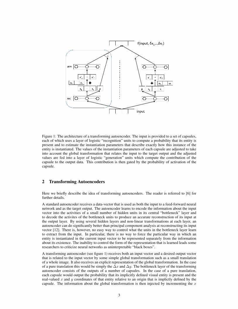
Figure 1: The architecture of a transforming autoencoder. The input is provided to a set of capsules,each of which uses a layer of logistic “recognition” units to compute a probability that its entity ispresent and to estimate the instantiation parameters that describe exactly how this instance of theentity is instantiated. The values of the instantiation parameters of each capsule are adjusted to takeinto account the global transformation that relates the input to the target output and the adjustedvalues are fed into a layer of logistic “generation” units which compute the contribution of thecapsule to the output data. This contribution is then gated by the probability of activation of thecapsule.

2 Transforming Autoencoders

Here we briefly describe the idea of transforming autoencoders. The reader is referred to [6] forfurther details.

A standard autoencoder receives a data-vector that is used as both the input to a feed-forward neuralnetwork and as the target output. The autoencoder learns to encode the information about the inputvector into the activities of a small number of hidden units in its central “bottleneck” layer andto decode the activites of the bottleneck units to produce an accurate reconstruction of its input atthe output layer. By using several hidden layers and non-linear transformations at each layer, anautoencoder can do significantly better than principal component analysis at reconstructing its inputvector [12]. There is, however, no easy way to control what the units in the bottleneck layer learnto extract from the input. In particular, there is no way to force the particular way in which anentity is instantiated in the current input vector to be represented separately from the informationabout its existence. The inability to control the form of the representation that is learned leads someresearchers to criticize neural networks as uninterpretable “black boxes”.

A transforming autoencoder (see figure 1) receives both an input vector and a desired output vectorthat is related to the input vector by some simple global transformation such as a small translationof a whole image. It also receives an explicit representation of the global transformation. In the caseof a pure translation this would be simply the ∆x and ∆y. The bottleneck layer of the transformingautoencoder consists of the outputs of a number of capsules. In the case of a pure translation,each capsule would output the probability that its implicitly defined visual entity is present and thereal-valued x and y coordinates of that entity relative to an origin that is implictly defined by thecapsule. The information about the global transformation is then injected by incrementing the x

3

and y outputs of every capsule by ∆x and ∆y 1. The transforming autoencoder must then constructthe transformed image from the transformed capsule outputs. All of the weights in a transformingautoencoder are learned by backpropagating the derivatives of the misfit between the actual anddesired outputs. During the training phase, the different capsules learn to extract different entitiesor similar entities in different parts of the space of instantiation parameters in order to minimize themisfit between the final output and the target. It would also be straightforward to share recognitionand generation units between capsules

By explicitly injecting ∆x and ∆y, we encourage the transforming autoencoder to use the x and youtputs of each capsule to represent the real x and y coordinates of some visual entity. If it usesits x and y outputs in this way, it automatically produces the correct output image when the desiredoutput image is held constant but the input image is translated by n pixels in the x direction and the∆x input is reduced by n.

One limitation of using capsules that output a set of explicit instantiation parameters is that eachcapsule can only deal with zero or one instance of its visual entity at a time. So for entities that aredensely distributed the capsules need to operate over small domains in which there is generally notmore than one instance at a time. For more complex, rarer entities the domains can be much bigger,so in a system with multiple layers of capsules we would expect the higher-level capsules to havemuch bigger domains than the lower-level ones. This does not mean that the higher levels have lostthe information about the instantiation parameters (as they do in a multilayer convolutional net withsubsampling). Capsules with large domains can encode information about the precise position oftheir visual entity just as accurately as capsules with small domains.

Until now, transforming autoencoders have only been applied to images, but they are applicable toany domain in which we know how to apply global transformations to the data. Speech is an obviouscandidate.

2.1 A Way to Improve Transforming Autoencoders

We can further encourage a transforming autoencoder to use its capsule outputs in the desired wayby using the transformed data as an alternative input. The idea is that the instantiation parametersextracted from the original and the transformed inputs should differ by exactly the amount specifiedby the global transformation.

We explicitly enforced this property by adding the following regularization term for each type oftransformation.

Nc∑i=1

pi (v) {Ci (v) + ∂c− Ci (g (v, ∂c))}2 (1)

where Nc is the number of capsules, g (v, ∂c) is the result of applying transformation g (·, ·) to vec-tor v using parameter ∂c, pi (v) and Ci (v) are the probability and the output respectively, of capsulei for data v. This regularization term requires the capsule values to be equivariant to transformationsof the data. i.e. if a transformation of ∂c was applied to the input data, the instantiation parametercomputed by each capsule must also transform by ∂c if pi (v) is significant. The regularization isused only to adjust the parameters related to the computation of the instantiation parameters, not tothe computation of the capsule probabilities. Doing the latter resulted in much poorer models whereequivariance of the generative features was strongly limited.

2.2 Sampling of Capsules

Since our aim is to use capsules to capture acoustic events, we wanted to train a stochastic trans-forming autoencoder in which the capsules were either active or inactive for a particular input. Suchbinary activities should prevent cooperation between different capsules in the creation of the recon-struction that may be possible with capsule activities that are more real valued. To achieve this, thecapsule activation states were sampled from their logistic probabilities. If the capsules were active,their outputs were added to the output of the transforming autoencoder, otherwise, their outputs wereignored. The error function being optimized was the expected error of reconstruction. While it is

1In this paper, the global transformations of the instantiation parameters were randomly generated for everydata case.

4

(a)

(b)

0.0

0.9

(c)

(d)

(e)

(f)

(g)

(h)

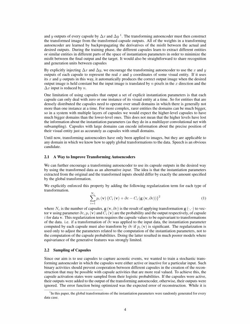
Figure 2: (a) 312.5 ms subsegment of an utterance. (b) Probabilities of activations of capsules. (c)Reconstruction of the utterance from the capsules (logistic outputs). (d,e,f, g, h) Contributions offive different capsules to the reconstruction.

simple to integrate out the states of the capsules in computing this error function and to compute thegradient with respect to the exact value, this involves terms that include all combinations of pairs ofcapsule states. So, for this paper, we simply estimated this gradient using a single Monte Carlo sam-ple for each data point. Thus, for the capsules whose sampled states were on, the gradients from theoutput error were backpropagated through the capsules, otherwise they were not. In addition, for therecognition part of the autoencoder, gradients were also backpropagated to account for the changein probabilities of the states. We found that the stochastic transforming autoencoder could only betrained after using a deterministic transforming autoencoder with real-valued activities to initializethe weights. This is probably because the estimate of the gradient is very noisy when a single MonteCarlo sample of the activations is used early in the training when the activation probabilities aremostly near 0.5. Once the reconstruction error was low enough and the capsule activations hadless entropy, the estimated gradient became less noisy. Even so, in order to facilitate the learningof the stochastic transforming autoencoder we used a very small learning rate of .001 without anymomentum.

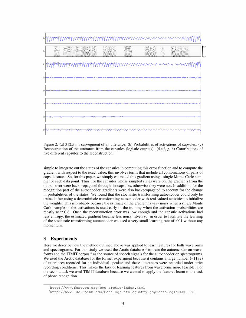
3 ExperimentsHere we describe how the method outlined above was applied to learn features for both waveformsand spectrograms. For this study we used the Arctic database 2 to train the autoencoder on wave-forms and the TIMIT corpus 3 as the source of speech signals for the autoencoder on spectrograms.We used the Arctic database for the former experiment because it contains a large number (=1132)of utterances recorded for an individual speaker and these utterances were recorded under strictrecording conditions. This makes the task of learning features from waveforms more feasible. Forthe second task we used TIMIT database because we wanted to apply the features learnt to the taskof phone recognition.

2http://www.festvox.org/cmu_arctic/index.html3http://www.ldc.upenn.edu/Catalog/CatalogEntry.jsp?catalogId=LDC93S1

5

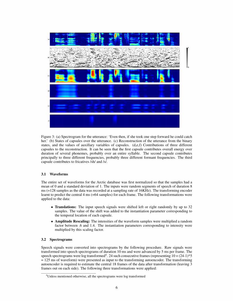
Figure 3: (a) Spectrogram for the utterance: ‘Even then, if she took one step forward he could catchher.’ (b) States of capsules over the utterance. (c) Reconstruction of the utterance from the binarystates, and the values of auxillary variables of capsules. (d,e,f) Contributions of three differentcapsules to the reconstruction. It can be seen that the first capsule contributes overall energy overduration of several phonemes, probably over an entire syllable. The second capsule contributesprincipally to three different frequencies, probably three different formant frequencies. The thirdcapsule contributes to fricatives /sh/ and /s/.

3.1 Waveforms

The entire set of waveforms for the Arctic database was first normalized so that the samples had amean of 0 and a standard deviation of 1. The inputs were random segments of speech of duration 8ms (=128 samples as the data was recorded at a sampling rate of 16KHz). The transforming encoderlearnt to predict the central 4 ms (=64 samples) for each frame. The following transformations wereapplied to the data:

• Translations: The input speech signals were shifted left or right randomly by up to 32samples. The value of the shift was added to the instantiation parameter corresponding tothe temporal location of each capsule.

• Amplitude Rescaling: The intensities of the waveform samples were multiplied a randomfactor between .6 and 1.4. The instantiation parameters corresponding to intensity weremultiplied by this scaling factor.

3.2 Spectrograms

Speech signals were converted into spectrograms by the following procedure. Raw signals weretransformed into speech spectrograms of duration 10 ms and were advanced by 5 ms per frame. Thespeech spectrograms were log transformed4. 24 such consecutive frames (representing 10 + (24-1)*5= 125 ms of waveform) were presented as input to the transforming autoencoder. The transformingautoencoder is required to estimate the central 18 frames of the data after transformation (leaving 3frames out on each side). The following three transformations were applied:

4Unless mentioned otherwise, all the spectrograms were log transformed

6

• Translations: The input frames of the spectrogram were shifted left or right randomly byup to three frames.• Scaling: The intensities of the spectrogram (before log transform) were scaled up or down

by a random factor between .1 and 10. This was achieved by generating a random numberbetween log(.1) and log(10) and adding it to the log spectrogram.

• Frequency Resampling: The log spectrograms were resampled in the frequency domainby a random rate between 0.8 and 1.2. The frequency resampling was achieved by firstperforming a cubic spline interpolation of each frame of the log spectrogram as a functionof frequency, and then interpolating at integer multiples of the resampling rate.

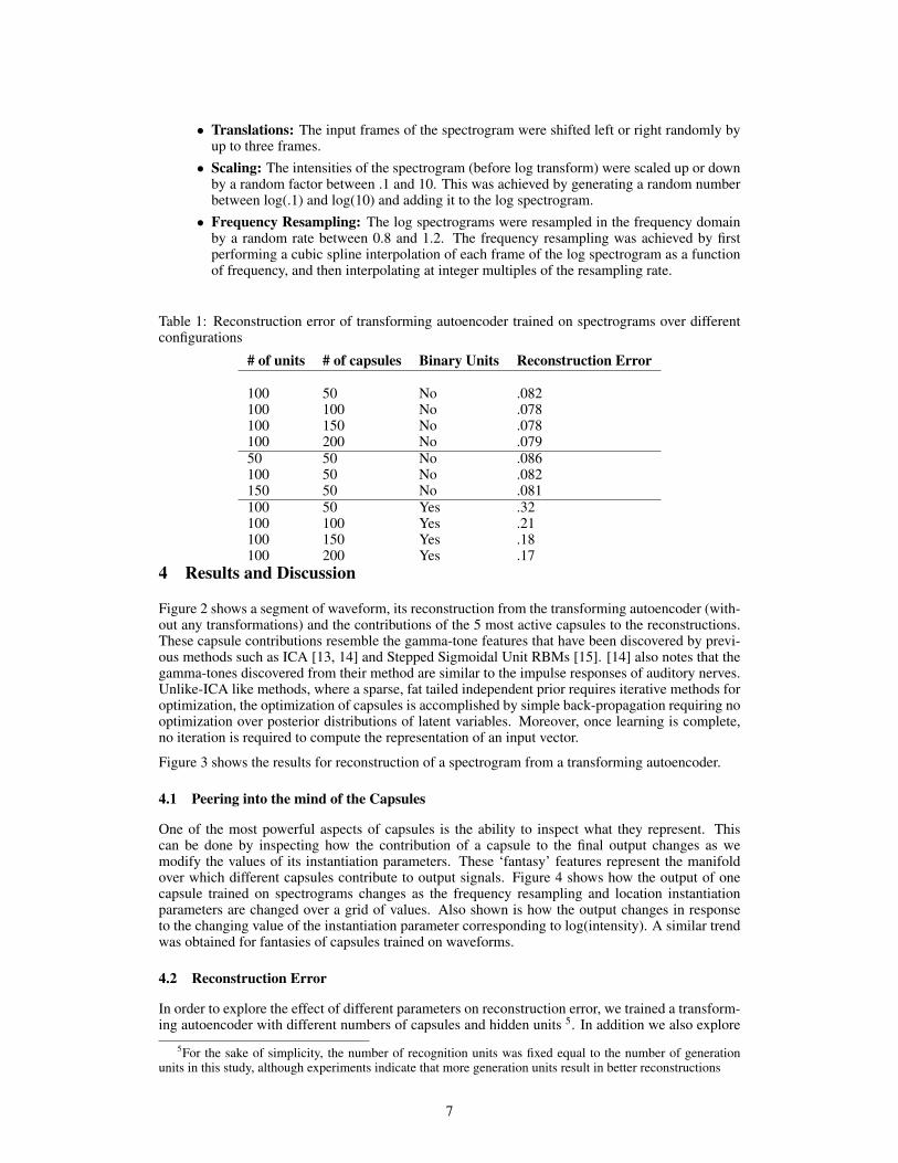
Table 1: Reconstruction error of transforming autoencoder trained on spectrograms over differentconfigurations

# of units # of capsules Binary Units Reconstruction Error

100 50 No .082100 100 No .078100 150 No .078100 200 No .07950 50 No .086100 50 No .082150 50 No .081100 50 Yes .32100 100 Yes .21100 150 Yes .18100 200 Yes .17

4 Results and Discussion

Figure 2 shows a segment of waveform, its reconstruction from the transforming autoencoder (with-out any transformations) and the contributions of the 5 most active capsules to the reconstructions.These capsule contributions resemble the gamma-tone features that have been discovered by previ-ous methods such as ICA [13, 14] and Stepped Sigmoidal Unit RBMs [15]. [14] also notes that thegamma-tones discovered from their method are similar to the impulse responses of auditory nerves.Unlike-ICA like methods, where a sparse, fat tailed independent prior requires iterative methods foroptimization, the optimization of capsules is accomplished by simple back-propagation requiring nooptimization over posterior distributions of latent variables. Moreover, once learning is complete,no iteration is required to compute the representation of an input vector.

Figure 3 shows the results for reconstruction of a spectrogram from a transforming autoencoder.

4.1 Peering into the mind of the Capsules

One of the most powerful aspects of capsules is the ability to inspect what they represent. Thiscan be done by inspecting how the contribution of a capsule to the final output changes as wemodify the values of its instantiation parameters. These ‘fantasy’ features represent the manifoldover which different capsules contribute to output signals. Figure 4 shows how the output of onecapsule trained on spectrograms changes as the frequency resampling and location instantiationparameters are changed over a grid of values. Also shown is how the output changes in responseto the changing value of the instantiation parameter corresponding to log(intensity). A similar trendwas obtained for fantasies of capsules trained on waveforms.

4.2 Reconstruction Error

In order to explore the effect of different parameters on reconstruction error, we trained a transform-ing autoencoder with different numbers of capsules and hidden units 5. In addition we also explore

5For the sake of simplicity, the number of recognition units was fixed equal to the number of generationunits in this study, although experiments indicate that more generation units result in better reconstructions

7

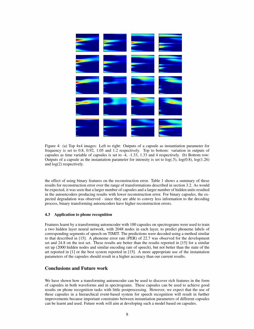
Figure 4: (a) Top 4x4 images: Left to right: Outputs of a capsule as instantiation parameter forfrequency is set to 0.8, 0.92, 1.05 and 1.2 respectively. Top to bottom: variation in outputs ofcapsules as time variable of capsules is set to -4, -1.33, 1.33 and 4 respectively. (b) Bottom row:Outputs of a capsule as the instantation parameter for intensity is set to log(.5), log(0.8), log(1.26)and log(2) respectively.

the effect of using binary features on the reconstruction error. Table 1 shows a summary of theseresults for reconstruction error over the range of transformations described in section 3.2. As wouldbe expected, it was seen that a larger number of capsules and a larger number of hidden units resultedin the autoencoders producing results with lower reconstruction error. For binary capsules, the ex-pected degradation was observed - since they are able to convey less information to the decodingprocess, binary transforming autoencoders have higher reconstruction errors.

4.3 Application to phone recognition

Features learnt by a transforming autoencoder with 100 capsules on spectrograms were used to traina two hidden layer neural network, with 2048 nodes in each layer, to predict phoneme labels ofcorresponding segments of speech on TIMIT. The predictions were decoded using a method similarto that described in [15]. A phoneme error rate (PER) of 22.7 was observed for the developmentset and 24.8 on the test set. These results are better than the results reported in [15] for a similarset up (2000 hidden nodes and similar encoding rate of speech), but not better than the state of theart reported in [1] or the best system reported in [15]. A more appropriate use of the instantationparameters of the capsules should result in a higher accuracy than our current results.

Conclusions and Future work

We have shown how a transforming autoencoder can be used to discover rich features in the formof capsules in both waveforms and in spectrograms. These capsules can be used to achieve goodresults on phone recognition tasks with little postprocessing. However, we expect that the use ofthese capsules in a hierarchical event-based system for speech recognition will result in furtherimprovements because important constraints between instantiation parameters of different capsulescan be learnt and used. Future work will aim at developing such a model based on capsules.

8

References

[1] Dahl, G., Ranzato, M., Mohamed, A. and Hinton, G. E. (2010) Phone Recognition with the Mean-Covariance Restricted Boltzmann Machine. Advances in Neural Information Processing 23:469-477

[2] Hinton, G. E., Osindero, S. and Teh, Y. (2006) A fast learning algorithm for deep belief nets. NeuralComputation 18:1527-1554.

[3] Vincent, P., Larochelle, H., Bengio, Y. and Manzagol, P. A. (2008) Extracting and Composing RobustFeatures with Denoising Autoencoders. Proceedings of the Twenty-fifth International Conference on MachineLearning:1096 - 1103

[4] LeCun, Y., Bottou, L., Bengio, Y. and Haffner., P. (1998) Gradient-based learning applied to documentrecognition. Proceedings of the IEEE 86:22782324

[5] Hinton, G. E., McClelland, J. L., and Rumelhart, D. E. (1986) Distributed representations. In Rumelhart,D. E. and McClelland, J. L., editors, Parallel Distributed Processing: Explorations in the Microstructure ofCognition. Volume 1: Foundations:77-109. MA: MIT.

[6] Hinton, G. E., Krizhevsky, A. and Wang, S. (2011) Transforming Auto-encoders. ICANN-11: InternationalConference on Artificial Neural Networks; preprint (2011)

[7] Stevens, K.N. (1972) The quantal nature of speech: Evidence from Articulatory-Acoustic data. In P. B.Denes and E. E. David Jr., editors, Human Communication: A Unified View: 51-66. NY: McGraw-Hill.

[8] Chistovich, L. A. and Lublinskaya, V. V. (1979) The center of gravity effect in vowel spectra and critical dis-tance between the formants: Psychoacoustical study of the perception of vowel-like stimuli. Hearing Research1:(3):185-195.

[9] Delgutte B. and Kiang, N. Y. (1984) Speech coding in the auditory nerve: IV. Sounds with consonant-likedynamic characteristics. Journal of the Acoustical Society of America 75(3):897-907

[10] Clements, G.N. (1985) The geometry of phonological features. Phonology 2:225-252.

[11] Jansen, A. (2011) Whole word discriminative point process models. Proceedings of the InternationalConference on Acoustics, Speech and Signal Processing 2011; preprint(2011)

[12] Hinton, G. E. and Salakhutdinov, R. R. (2006) Reducing the dimensionality of data with neural networks.Science 313(5786):504 - 507

[13] Lee, J., Jung, H., Lee, T., and Lee, S. (2000) Speech feature extraction using independent component anal-ysis. Proceedings of the International Conference on Acoustics, Speech and Signal Processing 2000 3(3):1631-1634.

[14] Lewicki, M.S. (2002) Efficient coding of natural sounds. Nature Neuroscience 5(4):356-363.

[15] Jaitly, N. and Hinton, G. E. (2011) Learning a better Representation of Speech Sound Waves using Re-stricted Boltzmann Machines. Proceedings of the International Conference on Acoustics, Speech and SignalProcessing 2011; preprint (2011)

9