A non-interactive methodology to assess farmers' utility ...aoatools.aua.gr/pilotec/files/bibliography/Amador_Sumpsi_Romero... · A non-interactive methodology to assess farmers

A non-interactive methodology to assess farmers' utilityfunctions: An application to large farms in

Andalusia, Spain

FRANCISCO AMADORBusiness School, ETEA, Cdrdoba, Spain

JOSE MARIA SUMPSI and CARLOS ROMEROTechnical University of Madrid, Spain

(received July 1996, final version received September 1997)

Summary

This paper proposes a methodological approach for eliciting farmers' utilityfunctions. The methodology is non-interactive, in that the parameters definingthe utility function are obtained by observing the actual behaviour adopted byfarmers without resorting to the use of questions on random lotteries. Themethodology recognises that the farmer attempts to achieve several objectives,most of which are in conflict. The methodological approach is applied to alarge farmer in the county of Vega de Cdrdoba, Spain. The primary empiricalfinding of this research was a satisfactory explanation of farmers' behaviourthrough a multi-attribute utility function with three attributes: working capital,risk and level of relative profitability.

Keywords: farmers' goals, utility function, multi-criteria analysis, goalprogramming.

1. Introduction

Nowadays, it is well accepted that multiple objectives are the rule ratherthan the exception in the agricultural field when decisions are taken at thefarm or regional level (see Gasson, 1973; Cary and Holmes, 1982; Romero

* The authors wish to thank the three reviewers and the Editor for helpful comments onearlier versions of this paper. The English editing by Christine Mendez is appreciated. Apreliminary version of this paper was presented at the 8th European Congress of AgriculturalEconomists held in Edinburgh, U.K., September 1996.

European Review of Agricultural Economics 0165-1587/98/0025-009225 (1998) 92-109 © Walter de Gruyter, Berlin

Non-interactive methodology to assess farmers' utility functions 93

and Rehman, 1989; Dent and Jones, 1993, and a large body of other litera-ture). Once the multiplicity of objectives in agriculture is accepted, there aretwo main approaches to building decision-making models.

The first and most rigorous direction consists in defining a utility functioncomprising all relevant objectives for a given decision problem. This kind ofmethodology, known as Multi-Attribute Utility Theory (MAUT), was chieflydeveloped by Keeney and Raiffa (1976). MAUT is a theoretically soundapproach based on the assumption of rationality underlying the classic para-digm of expected utility created by Von Neumann and Morgenstern (1944).However, its applicability poses many difficulties, as is explained below. Thus,very few applications of MAUT in the agricultural field can be reported (e.g.,Herath, 1981; Delforce and Hardaker, 1985; Foltz et al, 1995).

The second direction consists in looking for multi-criteria approacheswithout the theoretical soundness of MAUT, but which can accommodatein a realistic manner the multiplicity of criteria inherent to most agriculturalplanning problems. Among the possible surrogates of MAUT, the mostwidely used in the agricultural field are: goal programming, multi-objectiveprogramming and compromise programming. Rehman and Romero (1993)analyse the pros and cons of these surrogates in agriculture.

A major problem associated with the formulation of MAUT models liesin the high degree of interaction with the decision maker required by thismethodology. This issue is particularly important in agriculture where thecultural background of the decision maker is often not the most suitable forundertaking such an interactive process. Thus, within the context of apeasant economy, to question the person in charge of a family farm thor-oughly about his/her preferences concerning different random lotteries inorder to test independence conditions or assess individual utility functionscan be a very indecisive process.

This paper presents a pragmatic methodology capable of assessing afarmer's utility function. The proposed approach does not require any kindof interaction with the decision maker, but rather an awareness of the actualbehaviour followed by the farmer. In other words, it attempts to obtain autility function consistent with preferences revealed by farmers themselves.A drawback of the method is that revealed preference can be distorted byfactors not under control of the farmer (see end of Section 3).

The next section examines the main problems associated with the implemen-tation of the MAUT approach, especially in agricultural applications. Thepaper then uses our non-interactive approach to assess the utility function ofa big farmer in the county of Vega de Cordoba in Andalusia, Spain.

2. The classic implementation of a MAUT model: Some criticisms in theagricultural field

The classic assessment of a MAUT model requires the implementation offive basic steps, which can be summarised as follows (Zeleny, 1982:419-431):

94 Francisco Amador et al.

1. To train the decision maker in the terminology, concepts and techniquesto be used.

2. To test the corresponding independence conditions in order to justifythe appropriate functional form of the multi-attribute utility function(additive, multiplicative, etc.).

3. To assess the individual utility functions for each objective relevant tothe corresponding decision problem.

4. To estimate the weights and scaling constants associated with eachutility function. Once the values of these parameters and their corre-sponding functional form (step 2) are known, then the individual utilityfunctions can be amalgamated into an aggregate multi-attribute utilityfunction.

5. To test the consistency of the results obtained.The last four steps require notable interaction with the decision maker

as several artificial random lotteries requesting values of outcome whichsecure certain indifference statements are presented to him/her. These kindsof questions are not easy to answer. Moreover, as some researchers havepointed out, the MAUT methodology assumes a priori that decision makersevaluate lotteries as if they are maximising expected utility. Consequently,there is a certain circularity within the MAUT approach.

Indeed, some of the procedural steps demand from the decision makernot only answers to difficult questions but a large number of answers. Thus,to estimate the values of the scaling constants in a multiplicative functionalform, where the additive independence condition does not hold, requiresanswers to 2q-\ questions, where q is the number of objectives under consider-ation, i.e. for 5 objectives - not an uncommon situation in agriculture -elicitation of the scaling constants requires formulating and obtaininganswers to 31 statements based upon random lotteries!

For these reasons, the pragmatic value of the MAUT approach is limitedto problems with few objectives (at most two or three) and with an importanteconomic relevance, such as the location of an airport or a nuclear powerplant. Within this context, the capacity and responsibility of the decisionmaker makes it possible to implement such a complex interactive process.

It is obvious that the application possibilities of the traditional MAUTapproach are scarce in the agriculture field. To establish such an exhaustiveinteraction with a subsistence farmer or even a commercial farmer in orderto elicit their utility function does not seem advisable. The next sectiondemonstrates how it is possible to elicit this kind of utility function withoutthe need to interact with the decision maker. In this way, by preserving thebasic theoretical underpinning of the classic utility optimisation, a multi-attribute utility function consistent with the actual preferences shown byfarmers will be obtained. In short, the information necessary to assess theutility function will be obtained by observing actual behaviour rather thanby posing complex questions to farmers.


It should be emphasised that this paper does not claim the superiority ofthe proposed method with respect to MAUT. The latter remains the theoreti-cally correct method to follow when a strong interaction with the fanner ispossible.

3. Methodology

The first step in the methodology corresponds to a previous study (Sumpsiet al., 1993, 1997) where weights indicating the relative importance to beattached to the objectives followed by a farmer are elicited. The 'best' weightsare those compatible with the preferences revealed by the farmer beinganalysed. For this task and the new methodological proposal, the followingnotation is used:x = vector of decision variables (i.e., area covered by each crop)F = feasible set (i.e., the set of constraints imposed on the model)/; (x) = mathematical expression of the i-th objectiveW; = weight measuring relative importance attached to the i-th

objective/*; = ideal or anchor value achieved by the i-th objective/ i + = anti-ideal or nadir value achieved by the i-th objectivef = observed value achieved by the i-th objectivefj = value achieved by the i-th objective when the j-ih objective is

optimisedn,- = negative deviation, i.e. the measurement of the under-achievement

of the i-th objective with respect to a given target.Pi = positive deviation, i.e. the measurement of the over-achievement of

the i-th objective with respect to a given target.The first step consists of defining a tentative set of objectives /i(x), ...

/i(x), ...fq(\) which seeks to represent the actual objectives followed by thefarmer. The second step consists of determining the pay-off matrix for theabove objectives. The elements of this matrix are obtained by optimisingeach objective separately over the feasible set and then computing the valueof each objective at each of the optimal solutions [see Sumpsi et al. (1997)for technical details about the design and construction of the pay-off matrix].

Once the pay-off matrix is obtained, the following system of q equationsis formed:

T. 7 = 1


The last condition of (1) is not essential and is introduced only to normal-ise the weights Wj. If this system of equations has a non-negative solution,this will represent the set of weights to be attached to each objective, andthus the actual behaviour ( / i , /2 , . . . , / , ) followed by the farmer is reproduced.In most cases, an exact solution does not exist. In other words, there is noset of weights wl5 w2, ..., wq capable of reproducing the actual preferencesrevealed by the farmer. Consequently, the best solution of (1) is sought. Thisproblem can be considered equivalent to a regression analysis case where/-are the endogenous variables and/J,- the exogenous one. Among the possiblecriteria for minimising the corresponding deviations, and given our preferen-tial context, the following are proposed:

The Lx criterion. With this approach, the sum of positive and negativedeviational variables is minimised. This criterion underlies the use of metric 1.As is well known since Charnes et al. (1955), this kind of regression analysisproblem can be formulated in terms of goal programming (GP), as follows(see also, Ignizio, 1976; Romero, 1991):

M » n Z ji = l \ Ji /

subject to:

Z wjfij+ni-Pi=fi ' = 1> 2 . •••> 1(2)

It should be remarked that GP is not used here as a 'satisficing' decision-making approach, and, as such, the right-hand-side values do not representproper targets. In this paper, GP is simply used as a mathematical deviceto approximate a solution for an unfeasible system of equations such as (1)where the right-hand sides are the values achieved by the objectives underconsideration.

From a preferential point of view, the hx criterion is consistent with aseparable and additive utility function (see, e.g., Dyer, 1977). That is, weightsobtained from (2) lead to the following utility function:

i W-«=Z-ri/<M (3)

where kt is a normalising factor (e.g., ideal minus anti-ideal values; i.e.

The L^ criterion. With this approach, the largest deviation D is minimised.This criterion underlies the use of metric oo and the corresponding regression


analysis problem can be formulated in terms of linear programming (LP)as follows (see Appa and Smith, 1993):

Min D, subject to:

(4)

It has been proved elsewhere (Ballestero and Romero, 1991) that model(4) implies the following chain of equalities:

r̂ t *jfu-f\=^qLj=l

(5)

That is, from a preferential point of view, the Lx criterion implies aperfectly balanced allocation between the differences given by the prediction

I wjfuJ=I

and the value observed for/f in the q objectives considered. The correspond-ing utility contours are represented in Figure 1 for a bi-criterion case. This

CM

c

1O

Direction of improvement

Direction of improvement

Contours of aTchebycheff function

Contours of anaugmented Tchebychefffunction

Objective function 1 'i

Figure 1. Utility contours for a Tchebycheff and an Augmented Tchebycheff function(bi-criteria case)


kind of utility function, in the operational research literature, is called aTchebycheff or maximin function for which the largest deviation is minimised(see Steuer, 1989).1 This structure of preferences leads to the following utilityfunction:

^ ^ J (6)The above utility function does not imply separability among objectives

but a perfect complementary relationship between them (see again Figure 1).On the other hand, function (6) is not smooth and hence its maximisationis performed by solving the following equivalent problem (e.g., Nakayama,1992):

Min D subject to:(7)

jUf-fMl^D i=l,2, ... q

A compromise between L1 and Lx. With this approach, a compromisebetween minimising the sum of deviational variables and minimising thelargest deviation is sought. This aggregate criterion attempts to take advan-tage of both approaches (Lewis and Taha, 1995). The corresponding problemis formulated in terms of LP as follows:

subject to:

(8)

Weights obtained from (8) lead to the following utility function:

(9)

If X is very large, u becomes an additive and separable utility function[see expression (3)], whereas for A = 0, u becomes a Tchebycheff function[see expression (6)]. For small values of A, u can be considered an augmented


Tchebycheff function. That is, the second term of (9) gives the utility contoursa 'certain slope'. Thus, if parameter X takes a small value, then (9) will leadto a well-balanced solution (an augmented Tchebycheff function) (seeFigure 1). However if the parameter X takes a large value, then (9) will leadto a solution close to the solution corresponding to the separable functiongiven by (3).2 Thus, depending on the value of parameter X, different utilityfunctions are generated. Again, the above utility function is not smooth.Consequently, its maximisation is performed by solving the following auxil-iary problem:

D-AEvViMi = l Ki

subject to:

l ^ C / f - . / M K D i= l ,2 , . . . , 9 (10)

The next step in our methodology involves determining the functionalform of the multi-attribute utility function which best approximates theactual situation. For this purpose, we only need to maximise alternativelyexpressions (3), (6) or (9) subject to the relevant constraint set and tocompare the results with the actual values achieved by the q objectives. Forinstance, for utility function (3) the following mathematical programmingproblem is formulated:

Max t ^/;(x)

subject to:

/•(x) + «i-pi=y; i=l,2,...,q

x e F

Similar mathematical programming problems are formulated for the otherutility functions. The preference structure which provides the solution closestto the actual situation will be considered the utility function consistent withthe preferences revealed by the farmer. If none of the utility functional formsexamined leads to consistent results, then other forms of utility functionshould be tried until the behaviour of the farmer is predicted with enoughaccuracy. By consistent results, we mean that there is a marked similaritybetween the predictions provided by the utility function chosen and theobserved values for each of the objectives. The similarity can be checkedusing a variety of statistics (see note 3).

It should be noted that the methodology proposed uses just one year'sdata. Therefore, it is crucial that the year chosen reflects a typical year forwhich stochastic variables are close to their expected values, otherwise biasedresults may be obtained.


4. Application

In this section, the methodology previously described is used to elicit theutility function of a farmer belonging to a homogeneous group of large-scale farmers in the county of Vega of Cordoba, Andalusia (Spain). Thecharacteristics of this group of farmers (farm size, cropping patterns, soilquality, etc), are similar (see Sumpsi et al., 1993) so one might hypothesisethat the behaviour of the different farmers in the group will follow a similarpattern; that is, the utility function elicited for the farmer being analysedcan also be used to reproduce accurately the behaviour of the other farmersin the group. This hypothesis will be checked.

To begin, we need to identify a set of tentative objectives. After preliminaryinterviews with farmers belonging to the group of farms studied, the followinglist of objectives tentatively reflect the economic goals of the correspond-ing farmers:

Direction ofimprovement

1. Gross margin Max.2. Working capital Min.3. Employment Min.4. Management difficulty Min.5. Risk (MOTAD) Min.

Gross margin A/f

6. The ratio —— 2 — M a x -Working capital

Gross margin is an indicator of absolute profitability and is measured inmillion ptas. Working capital is measured in thousand ptas. Employmentrefers to the amount of labour required by the different crops each year andis measured in hours. Management difficulty is a qualitative index, definedby the authors, and is measured on a scale from 1 to 10 for each crop. Riskis incorporated according to the MOTAD method (Hazell, 1971). The ratiogross margin/working capital is a measure of relative profitability.

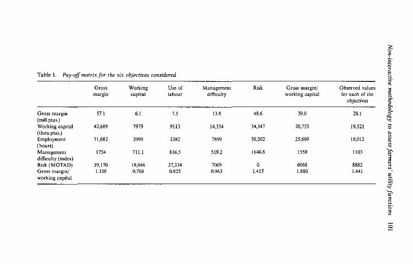
The next step was to determine the pay-off matrix for the farmer analysed.In order to do so, a mathematical model representing the farmer's decision-making environment was built. The model includes, along with the sixobjectives, a feasible region F which takes into account different constraints,including different types of land and availability for each type, standardagronomic practices adopted by farmers, cash-flow limits, capital investmentlimits and labour use in different time periods. For our data, the pay-offmatrix in Table 1 was obtained.

The last column of Table 1 is not actually a part of the pay-off matrix. Ithas only been added to show the observed value of each objective for the

rTable 1. Pay-off matrix for the six objectives considered a

Grossmargin

Workingcapital

Use oflabour

Managementdifficulty

Risk Gross margin/working capital

Observed valuesfor each of the

objectives s-o§•

foa

Gross margin(mill.ptas.)Working capital(thou.ptas.)Employment(hours)Managementdifficulty (index)Risk (MOTAD)Gross margin/working capital

57.1

42,689

71,682

1754

39,1701.338

6.1

7979

3999

711.1

18,6460.768

7.5

9113

3382

836.5

37,3340.825

13.8

14,354

7899

519.2

70090.963

48.6

34,347

50,202

1646.8

01.415

39.0

20,753

25,699

1559

60681.880

28.1

19,521

16,012

1103

88821.441

c


farm considered. Once the pay-off matrix has been obtained, the followingsystem of equations is formulated:

57.1 w,+ 6.1 w2+ , 7 . 5 H > 3 + 13.8 W4 + 48.6 W5 + 39.0 w6= 28.1

42,689 w,+ 7,979 w2+ 9,113 w3 + 14,354 w4

48.6 W5 + 39.0 w6

34,347 w5+ 20,753 w6= 19,521

71,682w,+ 3,999w2 + 3,382w3+ 7,899 w4+ 50,202w5+ 25,699w6 = 16,012

l,754w,+ 711.1w2 + 836.5w3 + 519.2w4+ I,646.8w5+ I,558w6= 1,103

39,170 iv! + 18,646 wz+ 37,334 w3 +

1.338w,+ 0.768H>2 + 0.825w3+

7,009 w4

0.963 w4 + 1.415w5

6,068 w6= 8,882

1.880 w6= 1.441

w« = 1

(12)

The above system of equations does not have a non-negative solution, i.e.,there is no set of weights actually capable of reproducing the observed valuesfor each of the objectives. Therefore, an approximate solution is sought byresorting to (2), (4) and to the family of functions given by (8). The resultsobtained are shown in Table 2.

For a value of the parameter X less than 0.02, the compromise criterionprovides the same set of weights as the L^ criterion and for a value of theX parameter larger than 1.5, the compromise criterion provides the same setof weights as the Lt criterion. It is interesting to note that for the farmeranalysed, what matters is not gross margin per se but gross margin generatedper money unit of working capital (i.e., w1=0 and w6>0). This clash betweenabsolute and relative profitability has been observed in other agriculturalscenarios (e.g., Mendez-Barrios, 1995).

The next step in our procedure consists of inserting these weights in thecorresponding utility functions (3), (6) and (9). To facilitate calculation ofthe different utility functions, only weight values larger than 0.05 were

Table 2. Set of weights generated by different minimisation criteria

Gross margin (W,)Working capital (W2)Employment (H^)Managementdifficulty (W4)Risk (W5)Gross margin/working capital (W6)

L,00.310

00.190.50

£«,00.190.09

0.050.050.62

0.02 < y < 0.2500.240.08

0.050.080.55

Criterion

Compromise

0.25 s X ̂ 0.50 0.75 <A< 1.500.340

00.090.57

00.260

0.110.100.53

X>\.500.310

00.190.50


considered. In fact, the inclusion in the computation process of weights lessthan or equal 0.05 had a negligible effect on the numerical predictionsprovided by the model. When a weight is omitted, its value is allocatedproportionally to the values of the other weights. For instance, for theLx criterion, the weights used to build the different utility functions are:W l = w4 = w5=0, w2 = 0.21, w3 = 0.10 and w6=0.69.

The different utility functions were obtained by arithmetic calculation.These utility functions were optimised subject to the constraint set in orderto check their capacity to reproduce the observed reality [see (11) for theseparable and additive case]. The three utility functions which provideresults more consistent with the actual observed values are the following:

(a) Separable and additive utility functions (uj

u, = {-0.89/2(x)-0.49/5(x) + 44964/6(x)}

(b) Tchebycheff utility functions (u2)

u2= -[Max{0.61(/2(x)-7979), 0.15(/3(x)-3382), 62050(1.88-/6(x))}]

(c) Augmented Tchebycheff utility functions (X = 1.6) (u3)

rMax{0.89(/2(x)-7979), 0.49(/5(x)-0), 44964(1.88-/6(x))}"I"3 |_ +1.42/2(x) + 0.78/5(x)-71942/6(x) J

Table 3 shows the actual observed values for the six objectives considered,as well as the predictions generated by the three utility functions selected.

The rationale of Table 3 is to check that the objectives and weightsestimated in equation (12) are compatible with observed values. A similarcomparison could be carried out directly in equation (12) by analysing thevalues of the deviation variables. In short, the results in Table 3 allow us toconclude that the parameters of the utility function have been correctlyestimated.

The three 'best' utility functions chosen (i.e., uu u2 and M3) basically showthe same capacity to reproduce the reality observed.3 Finding several utilityfunctions with the same basic predictive power, rather than a single 'best'utility function, is not surprising. In fact, Koksalan and Sagala (1995:200-201) have rightly remarked that different utility functional forms inmany cases yield exactly the same optimum. For example, in Figure 2, theTchebycheff and linear utility functions yield exactly the same optimum.4

To validate the applicability of the results to other farmers in the group,we checked that the utility functions elicited were also able to reproducethese fanners' behaviour with a good degree of accuracy.5 In fact, theconsistency index for all the cases in the group of farmers analysed wasnever higher than 10 per cent (see note 3). This verification confirms theconjecture stated at the beginning of this section and reinforces the pragmatic

Table 3. Comparison between observed and predicted values

Objectives

Gross margin(million ptas.)Working capital(thousand ptas.)Employment(hours)Managementdifficulty (index)Risk (MOTAD)Gross margin/workingcapital (ratio)

Actualobserved

values

28.1

19,521

16,012

1103

88821.441

Predictionprovided by ul

28.1

22,552

16,012

1103

88821.250

Predictionprovided by u2

32.8

19,521

16,012

1103

88821.680

Predictionprovided by u3

30.8

19,521

16,012

1103

88821.580

Predictionprovided by max

gross margin

57.1

42,689

71,682

1754

39,1701.338

s

csO

&.


o

od)

O

Efficient frontier

V Contours of ax Tchebycheff

\ function

Contours of alinear function

Objective function 1 ^

Figure 2. A Thebycheff and a linear function leading to the same optimum (adaptedfrom Koksalan and Sagala, 1995: 201)

value of our analytical effort within an ex-ante policy analysis perspective.The last column in Table 3 shows the values achieved by each objective

when the traditional objective function that maximises the gross margin isused. It is obvious that there is no resemblance between the observed valuesfor each of the objectives and gross margin maximisation behaviour. In fact,for gross margin criterion the calculated consistency index was more than160 per cent! This result has important practical implications. Suppose thata mathematical programming model is built to evaluate the effects of differentagricultural policies for our homogeneous group of farmers. A conventionalchoice of the objective function (i.e., gross margin) would lead to erroneousresults. However, the choice of utility functions u1, u2 or u3 as objectivefunction would predict realistic behavioural responses to the policy changesfor the homogeneous group of farmers analysed.

5. Concluding remarks

From a methodological point of view, it is important to point out that,whereas in the MAUT approach it is crucial to test whether the elicitedutility function is consistent with the answers provided by the decisionmaker, within our non-interactive context, an equivalent crucial point is tocheck whether the elicited utility function is or not compatible with thebehaviour of the fanner observed. It is obvious that an 'as if methodologyunderlies this approach. This kind of philosophical underpinning is quitelicit in economics, especially when the task is to build mathematical


programming models for the evaluation of the effects of different agricul-tural policies.

Within an agricultural planning context, the proposed non-interactivemethodology seems more operational than the classic MAUT approach.However, when this kind of comparison is considered, certain doubts canarise. In fact, the implementation of our approach requires the definition ofa constraint set representing the farmers' decision-making environment.Indeed, as the first step in the proposed methodology shows, we need todefine the constraint set, which is obviously not an easy task. However, aspecific constraint set is also necessary with a MAUT approach if we wantto use the elicited MAUT function for ex-ante policy analysis, since we needto optimise this function over the feasible set.

From an empirical point of view, we want to emphasise that the resultsobtained clearly show how the fanner analysed has a behaviour compatiblewith a series of objectives which differ considerably from the traditionalobjective maximising the gross margin of the farm. The latter is the objectivefunction commonly used in most mathematical programming models, whichcan give rise to misleading results, especially if the model is used for ex-anteanalysis of agricultural policies.6

It should be noted that the methodology focuses on an individual farmer.However, for a homogeneous group of farmers, inferences about the groupcan be made in the following two cases: (a) the utility functions elicited areable to reproduce with a good degree of accuracy the behaviour of most ofthe farmers of the group or (b) the individual farmer analysed representsthe average farmer of the group.

Our analytical effort should not be considered a purely theoreticalexercise, as it is precisely in the evaluation of the effects of agriculturalpolicy measures that this research can reach its maximum point of interest.Indeed, one of the basic problems in the accuracy of ex-ante policy analysisfrom research based on mathematical programming models is the correctspecification of the objective function. However, to do this, it is necessaryfirst to identify farmers' utility functions that are consistent with theobserved reality.

It is important to notice that although we have worked with a variety ofutility functions, if none of these had provided consistent results, othersshould have been tried. In short, the approach proposed can be viewed asa powerful generator of empirically testable behavioural hypotheses. In fact,each of the utility functions used can be considered a behavioural hypothesis.The 'best' empirically corroborated hypothesis will correspond to the utilityfunction whose predictions are closest with respect to the observed valuesfor each objective (i.e., expressions uu u2 and M3 in our case study).

Finally, we want to point out that this paper does not claim that ourmethod is better than MAUT given that these approaches are to someextent non-comparable. MAUT is based on a philosophy of interaction with


the decision maker, while the method proposed here is non-interactive andis based upon observations of the farmers' actual behaviour. In conclusion,if the analyst is capable of establishing an effective interaction process withfarmers, then MAUT is the right approach. On the contrary, if this type ofinteraction is not possible, then MAUT should give way to approaches suchas the one proposed in this paper.

Notes

1. Within a welfare economics context, some authors refer to this function as Rawlsian (e.g.Johansson, 1992: 32-39) given the connections between it and the principles of justiceintroduced by Rawls (1973: 75-80). However, as the translation of Rawls' ideas from ethicsto economics is a controversial topic (see e.g. Roemer 1996: Chap. 5), we have decided todenominate these functions as Tchebycheff as is usual in the mathematical and operationalresearch literature.

2. We note that a similar function has been proposed by Steuer and Choo (1983) for interactivemulti-criteria analysis and by Wierzbicki (1982) as a basis for the reference pointmethodologies.

3. From a technical point of view, it is possible to measure the degree of closeness between thepredictions provided by functions u,, u2 and u3 and the actual observed values. This taskcan be undertaken by resorting to any statistical procedure for measuring the similaritybetween two sets of data. In our case, we calculate a consistency index based upon metric 1by adding the ratios: 100*|(observed value-predicted value)|/(observed value) for the sixobjectives considered and then dividing the corresponding sum by six. In this way, the indexcan be interpreted as the average percentage deviation between the observed and the pre-dicted values. Other consistency indices based on other metrics can also be used. In anycase, the degree of accuracy must be specified beforehand. In our application, the consistencyindex defined above was used with a maximum allowed error of 10 per cent. The predictionsprovided by u,, u2 and u3 embody errors of 2.9, 3.33 and 1.96 per cent, respectively. Theresults are robust with respect to the metric chosen. Thus, if metric 2 is used, the sameranking is obtained.

4. Stewart (1995), using a Monte Carlo simulation experiment, found that different multi-attribute utility functions yield similar results when the same set of weights is used. Thissuggests that the essential element of the procedure here involves the elicitation of preferen-tial weights rather than identifying the most appropriate functional form.

5. In fact, the predictions provided by the estimated utility functions u,, u2 and u3 werecompared with the observed values for all the farmers of the homogeneous group. With thispurpose, the consistency index defined in note 3 was calculated, obtaining that, in all thecases, the value of the index was lower than 10 per cent. Hence, this supports the applicabilityof the results to other farmers of the group.

6. Some specialists may be surprised by the assumption that the group of farmers analysedbehave 'as if' all had the same objectives. Yet, paradoxically, most of the mathematicalprogramming applications in agriculture reported in the literature assume in one way or inanother that all the farmers are gross margin maximisers, which does not seem to producemuch surprise among some specialists!

References

Appa, G. and Smith, C. (1993). On L[ and Chebyshev estimation. Mathematical Programming5: 73-87.


Ballestero, E. and Romero, C. (1991). A theorem connecting utility function optimization andcompromise programming. Operations Research Letters 10: 421-427.

Cary, J. W. and Holmes, W. E. (1982). Relationship among farmers' goals and farm adjustmentstrategies: Some empirics of a multidimensional approach. Australian Journal of AgriculturalEconomics 26: 114-130.

Charnes, A., Cooper, W. W. and Ferguson, R. (1955). Optimal estimation of executive compensa-tion by linear programming. Management Science 1: 138-151.

Delforce, R. J. and Hardaker, J. B. (1985). An experiment in multiattribute utility theory.Australian Journal of Agricultural Economics 29: 179-198.

Dent, J. B. and Jones, W. J. (1993). Editorial. Agricultural Systems 41: 235-237.Dyer, J. S. (1977). On the Relationship between Goal Programming and Multiattribute Utility

Theory. Discussion paper No. 69. Management Study Center, University of California, LosAngeles.

Foltz, J. C , Lee, J. G., Martin, M. A. and Preckel, P. V. (1995). Multiattribute assessment ofalternative cropping systems. American Journal of Agricultural Economics 77: 408-420.

Gasson, R. (1973). Goals and values of farmers. Journal of Agricultural Economics 24:521-537.

Hazell, P. B. R. (1971). A linear alternative to quadratic and semivariance programming forfarm planning under uncertainty. American Journal of Agricultural Economics 62: 53-62.

Herath, H. M. G. (1981). An empirical evaluation of multiattribute utility theory in peasantagriculture. Oxford Agrarian Studies 10: 240-254.

Ignizio, J. P. (1976). Goal Programming and Extensions. Lexington, MA: Lexington Books.Johansson, P. O. (1992). An Introduction to Modern Welfare Economics. Cambridge: Cambridge

University Press.Keeney, R. L. and Raiffa, H. (1976). Decisions with Multiple Objectives. New York: Wiley.Koksalan, N. M. and Sagala, P. N. S. (1995). An approach to and computational results on

testing the form of a decision maker's utility function. Journal of Multi-Criteria DecisionAnalysis 4: 189-202.

Lewis, R. P. and Taha, H. A. (1995). An investigation of the use of goal programming to fitresponse surfaces. European Journal of Operational Research 86: 537-548.

Mendez-Barrios, J. C. (1995). Intensification de la Cafeiculture chez les Petits Producteurs duGuatemala. Doctoral Thesis, Ecole Nationale Superiure Agronomique de Montpellier.

Nakayama, H. (1992). Trade-off analysis using parametric optimisation techniques. EuropeanJournal of Operational Research 60: 87-98.

Rawls, J. (1973). A Theory of Justice. Oxford: Oxford University Press.Rehman, T. and Romero, C. (1993). The application of the MCDM paradigm to the manage-

ment of agricultural systems. Agricultural Systems 41: 239-255.Roemer, J. E. (1996). Theories of Distributive Justice. Cambridge, MA and London: Harvard

University Press.Romero, C. (1991). Handbook of Critical Issues in Goal Programming. Oxford: Pergamon Press.—, Rehman, T. (1989). Multiple Criteria Analysis for Agricultural Decisions. Amsterdam:

Elsevier.Steuer, R. E. (1989). Multiple Criteria Optimization: Theory, Computation, and Application.

Krieger.— and Choo, E-M. (1983). An interactive weighted Tchebycheff procedure for multiple objective

programming. Mathematical Programming 26: 326-344.Stewart, T. J. (1995). Simplified approaches for multi-criteria decision making under uncertainty.

Journal of Multi-Criteria Decision Analysis 4: 246-258.Sumpsi, J. M., Amador, F. and Romero, C. (1993). A research on Andalusian farmers' objective:

methodological aspects and policy implication. 7th European Association of AgriculturalEconomists Congress, Stresa.

— (1997). On farmers' objectives: a multi-criteria approach. European Journal of OperationalResearch 96: 64-71.


Von Neumann, J. and Morgenstern, O. (1944). Theory of Games and Economic Behavior. NewJersey: Princeton University Press.

Wierzbicki, A. P. (1982). A mathematical basis for satisfying decision making. MathematicalModelling 3: 391-405.

Zeleny, M. (1982). Multiple Criteria Decision Making. New York: McGraw-Hill.

Carlos RomeroETS Ingenieros de MontesUnidad de EconomiaAvenida Complutense s/n28040 MadridSpain

Documents

A non-interactive methodology to assess farmers' utility ...aoatools.aua.gr/pilotec/files/bibliography/Amador_Sumpsi_Romero... · A non-interactive methodology to assess farmers