A Non-Maxima Suppression Method for Edge Detection …dev.ipol.im/~morel/Dossier_MVA_2011_Cours_Transparents_Documen… · ISSN 0249-6399 apport de recherche INSTITUT NATIONAL DE

ISS

N 0

249-

6399

appor t de r echerche

INSTITUT NATIONAL DE RECHERCHE EN INFORMATIQUE ET EN AUTOMATIQUE

A Non-Maxima Suppression Method for EdgeDetection with Sub-Pixel Accuracy

Frederic Devernay

N˚ 2724Novembre 1995

PROGRAMME 4

A Non-Maxima Suppression Method for EdgeDetection with Sub-Pixel Accuracy

Frederic Devernay

Programme 4 — Robotique, image et visionProjet Robotvis

Rapport de recherche n˚2724 — Novembre 1995 — 20 pages

Abstract: In this article we present a two dimensional edge detector which givesthe edge position in an image with a sub-pixel accuracy. The method presented heregives an excellent accuracy (the position bias mean is almost zero and the standarddeviation is less than one tenth of a pixel) with a low computational cost, and its im-plementation is very simple since it is derivated from the well-known Non-MaximaSuppression method [2, 4]. We also justify the method by showing that it gives theexact result in a theoretical one dimensional example. We have tested the accuracyand robustness of the edge extractor on several synthetic and real images and bothqualitative and quantitative results are reported in this paper.

Key-words: Low-level processing, Edge detection, Sub-Pixel, Differential prop-erties of curves.

(Resume : tsvp)

Unite de recherche INRIA Sophia-Antipolis

2004 route des Lucioles, BP 93, 06902 SOPHIA-ANTIPOLIS Cedex (France)

Telephone : (33) 93 65 77 77 – Telecopie : (33) 93 65 77 65

Detection de contours a une precision inferieure aupixel par une methode derivee de la NMS

Resume : Nous presentons un detecteur de contours bidimensionnels qui donnela position du contour dans une image a une precision inferieure au pixel. La me-thode presentee ici donne d’excellents resultats (la moyenne de l’erreur en positionest presque zero et son ecart type est d’a peine un dixieme de pixel) pour un couten calcul a peine superieur a une methode classique, et de plus son implantationest tres simple puisqu’elle est derivee de la methode classique de suppression desnon-maxima locaux (NMS) [2, 4]. Nous justifions egalement l’utilisation de cettemethode en montrant qu’elle donne le resultat exact dans le cas d’un contour mo-nodimensionnel. Nous avons teste la precision et la robustesse de cet extracteur decontours sur plusieurs types d’images, synthetiques et reelles, et rapportons ici desresultats a la fois qualitatifs et quantitatifs.

Mots-cle : detection de contours, sous-pixel, proprietes differentielles de courbes.

A NMS Method for Edge Detection with Sub-Pixel Accuracy 1

Contents

1 Introduction 2

2 On edge extraction 32.1 The NMS method . . . . . . . . . . . . . . . . . . . . . . . . . . . 32.2 The sub-pixel approximation . . . . . . . . . . . . . . . . . . . . . 3

3 Using the proposed improvements 7

4 Results 84.1 The test data . . . . . . . . . . . . . . . . . . . . . . . . . . . . . . 84.2 The different edge detection methods . . . . . . . . . . . . . . . . . 104.3 Edge position . . . . . . . . . . . . . . . . . . . . . . . . . . . . . 104.4 Edge orientation . . . . . . . . . . . . . . . . . . . . . . . . . . . . 124.5 Other results . . . . . . . . . . . . . . . . . . . . . . . . . . . . . . 15

5 Conclusion 15

RR n˚2724

2 Frederic Devernay

1 Introduction

Edge detection is now taken for granted by most of the computer vision people, likemany other basic tools of computer vision. Since a lot of work has already been donein early vision, people working on higher level features tend to use as input the re-sult of classic low level algorithms and think this is the only information they can getfrom the image data. In the case of edge detection we used to work on informationthat was given to within about a pixel, and then had to do some kind of regulariza-tion process on it, like polygonal or spline approximation. Both introduce a certainquantity of error, but whereas the approximation error can be chosen, the error on thedetected edge position is both fixed and not negligible, especially when one wants tocompute differential properties of image curves like orientation, Euclidean curvatureor even higher degree properties like affine or projective curvature. Some attemptswere made in edge detection at a sub-pixel accuracy a few years ago, for exampleA. Huertas and G. Medioni [11] used a refinement of the zero-crossing of Laplacianbut they did not give any results on the accuracy of the edge detection. A.J. Tababaiand O.R. Mitchell [14] did some interesting work in the one-dimensional case whichwas extended to two-dimensional images and seemed to work properly. An edge re-location mechanism is also given in [15] but the required implementation is rathercomplex. The best results in terms of accuracy [12] were obtained at a high compu-tational cost, because this involved local surface fitting on the intensity data, and theresults are not better than our method. In general, the different methods that havebeen proposed often end up requiring regularization, excessive computer power, orboth of them.

For these reasons we made a very simple enhancement of the classical local non-maxima suppression, that gives a much better estimate of the curve position (up towithin a tenth of a pixel) or the curve orientation without regularization, and at a verylow computational cost. Using this edge detector, we can also calculate higher orderdifferential properties of curves with much less regularization than when using oldermethods. Besides, this method can be easily integrated in an existing vision systemsince it is based on a classical and widely-used method.

We present and interpret a wide variety of results to compare this method withexisting edge detection methods. We also calculated in the most simple way the lo-cal edge orientation to show that the result of our method can also be used to easilycalculate differential properties of the edges.

INRIA


2 On edge extraction

2.1 The NMS method

This method is based on one of the two methods commonly used for edge detection,the suppression of the local non-maxima of the magnitude of the gradient of imageintensity in the direction of this gradient [8] (also called NMS), the other one beingto consider edges as the zero-crossings of the Laplacian of image intensity [10, 9].NMS consists of:

1. Let a point (x; y), where x and y are integers and I(x; y) the intensity of pixel(x; y).

2. Calculate the gradient of image intensity and its magnitude in (x; y).

3. Estimate the magnitude of the gradient along the direction of the gradient insome neighborhood around (x; y).

4. If (x; y) is not a local maximum of the magnitude of the gradient along thedirection of the gradient then it is not an edge point.

Usually for step 4 the neighborhood is taken to be 3 � 3 and the values of themagnitude are linearly interpolated between the closest points in the neighborhood,e.g. in Figure 1 the value at C is interpolated between the values at A7 and A8 andthe values at B between those at A3 and A4. We have also tried to use quadraticinterpolation to compute these (the value atAwould be interpolated between those atA7, A8, and A1 as in Figure 2) and compared the results with the linear interpolation.After this edge detection process one usually does hysteresis thresholding [2] on thegradient norm and linking to get chains of pixels.

2.2 The sub-pixel approximation

Our main improvement of the method is very simple and consists of only adding thissingle step to the NMS process:

� If (x; y) is a local maximum then estimate the position of the edge point in thedirection of the gradient as the maximum of an interpolation on the values ofgradient norm at (x; y) and the neighboring points.

RR n˚2724

4 Frederic Devernay

A1

Ag

A2 A3

A4

A5A6A7

A8

B

C

Figure 1: Checking whether pixel A is a local maximum of the magnitude of the gra-dient in the direction of the gradient is done by interpolating the gradient magnitudeat B and C.

0−1 1

A

B

x

Figure 2: Examples of linear (A) and quadratic (B) interpolation between three val-ues at �1, 0, and 1.

INRIA


This is the principle, but we still have to find the interpolation between gradientnorm values we should apply to find the best position of the edge. We will considera simple quadratic interpolation of the values of the gradient norm between the 3values we have in the gradient direction. One could also try to locally fit a simplesurface (e.g. bi-quadratic) on the neighborhood of the considered point but we wantto keep the computations as simple as possible so that the implementation is fast andeasy.

The choice of the quadratic interpolation to find the maximum can be justifiedbecause it gives the exact result in the one-dimensional case. Let L = fl(i)ji 2 @gan infinite line of pixels with a step edge at position ��1

2, coordinate 0 corresponding

to the middle of pixel l(0). The continuous intensity function for this step edge, asshown in Figure 3, is:

I(t) =

(0 if t > � � 1

2

1 otherwise

so that

l(i) =R 1

2

�1

2

I(t)dt

l(�1) = � � � = l(�2) = l(�1) = 1

l(0) = �; 0 � � � 1

l(1) = l(2) = � � � = l(+1) = 0

I(t)

l(i)

t

i

Figure 3: A one-dimensional step edge and the corresponding gray-level pixel line.

Let r be a general derivation operator. It can be a finite differences operator, orany gradient filtering operator, the only constraint being that r is antisymmetric. Itcan be written:

rl(i) =+1Xk=1

gk(l(i+k)�l(i�k)) = � � ��g2l(i�2)�g1l(i�1)+g1l(i+1)+g2l(i+2)+� � �

RR n˚2724

6 Frederic Devernay

Let us apply this general derivation operator on locations �1; 0; 1:

rl(�1) = � � � � g2 � g1 + g1 � = C � (1� �) g1

rl(0) = � � � � g2 � g1 = C � g1

rl(1) = � � � � g2 � g1 � = C � � g1

where

C = �1Xk=2

gk

Since shifting and rescaling the values of the three points used to find a maximumof the quadratic interpolation do not affect the position of this maximum, we cansimplify things by using C = 0 and g1 = 1:

a = jrl(�1)j = 1� �

b = jrl(0)j = 1

c = jrl(1)j = �

Considering that the center of the pixels correspond to integer x coordinates, onecan find that the x position of the maximum of the parabola passing through (�1; a),(0; b), and (1; c) is:

m =a� c

2(a� 2b+ c): (1)

It can be easily seen that when b � a and b � c this value is bounded:

�0:5 � m � 0:5

Since integer coordinates correspond to pixel centers and pixel width is 1, this meansthat the sub-pixel position of an edge point will always be inside the pixel.

That gives in this case

m = � �1

2

which is exactly the theoretical position of the edge! Equation 1 shows that the edgeposition is invariant to additive and multiplicative changes in the data. Moreover,this result can be extended to any kind of smooth edge, since a smooth edge is theresult of the convolution of a step edge with a symmetric blurring operator s. The

INRIA


blurring operator s is symmetric so the action of the derivation on the ramp edge isthe same as the action of the convolution of this operator with the blurring operator,which can be considered as another derivating operator, on the corresponding stepedge:

r(s � l)(i) = (r � s)l(i) = r0l(i)

We should be careful about one thing with the previous computations: we workedwith the gradient norm, whereas most people might want to use the squared gradientnorm for NMS because it requires less calculations and when the squared gradientnorm is a local maximum the gradient norm is one too. But the quadratic interpo-lation gives a different result, and in the previous case we would find the maximumat:

m =1� 2�

4�2 � 4�� 2

which introduces a bias on the edge position. The maximum of the bias is �m =0:073 pixels at � = 0:19 and its standard deviation is �(�m) = 0:052, that is morethan 1

20pixel (the same magnitude order as the precision we would like to get). In

conclusion, using the squared gradient norm may reduce significantly the precisionof the edge extraction.

The comparison between the detected and the theoretical edge position was notdone in the two dimensional case because it involves too many parameters (includ-ing the position and angle of the edge, the coefficients of a generic two-dimensionalderivating filter, and the way the values a and c are calculated). Before seeing someresults let us see how this edge detector can be used in a classic image processingchain.

3 Using the proposed improvements

The main advantage of this new method over the sub-pixel edge detectors that havealready been done is that its cost in terms of calculation is almost nothing (3 additionsand 3 multiplications at each detected edge point if we use the quadratic approxima-tion, which make 6 floating-point operations, not including the computation of thegradient) and it can be easily integrated in a simple and well-known algorithm.

RR n˚2724

8 Frederic Devernay

The new problem that can appear with a sub-pixel edge detector is that becausethe point coordinates are not integer we may not be able to apply common techniquessuch as hysteresis thresholding or linking. Hopefully we have solved this problemthe simplest way we could: with this edge detector an edge point has non integercoordinates but can still be attached to the point from which it was calculated, whichhas integer coordinates. Thus we perform the common operations on the edge pointsas if they had integer coordinates, like hysteresis thresholding [2] using the gradientnorm and edge pixels linking, but can use their sub-pixel approximation wheneverwe want it, e.g. when we need the precise position or want to use some differentialproperties of the edge.

The solution we used is to save the sub-pixel position of each edge point sepa-rately when the edge detection process is finished, as (�x(x; y); �y(x; y)) pairs wherex and y are integers and (�x; �y) 2 [�0:5; 0:5] � [�0:5; 0:5], to do the other edgeprocesses on the other data that has been saved (the edge position up to within a pixeland the gradient norm), and to use the sub-pixel edge position when we need it laterin the processing.

In conclusion of this section, we say that one can use this new approach to greatlyimprove already existing algorithms with only minor modifications in the image pro-cessing chain.

4 Results

4.1 The test data

It seems to us that the qualities that should have a good edge detector are:

1. A good estimate on the position of the edge, whatever the edge position, ori-entation and curvature.

2. Good differential properties of the edge data, i.e. the edge orientation shouldnot be biased and have a small variance, and higher order differential proper-ties should be calculated accurately with not too much regularization.

3. All these properties should be robust to noise.

To verify these we used test data consisting of two series of images, each oneconsisting of a single edge:

INRIA


� A collection of lines, with light gray on one side and dark gray on the otherside, with a wide variety of orientations.

� A collection of filled circles with radiuses going from 3 to 100 pixels.

These are 128 � 128 images generated with anti-aliasing, the edge contrast isgiven (we chose 100 for our experiments), and uncorrelated Gaussian noise can beadded on the image intensity data. The anti-aliasing can be justified by the fact thatcommon image sensors (e.g. CCD) give the integral of light intensity over eachpixel. Two smaller sample images are shown Figure 4 to demonstrate what the anti-aliased and noisy images look like. We calculated the gradient of image intensity

Figure 4: Two 64 � 64 images of the same kind as the ones that were used for ourexperiments: A line at 22:50 with no noise and a circle of radius 20 with Gaussianadditive noise. The noise standard deviation is 50 which corresponds to a signal tonoise ratio (SNR) of 0dB.

using a Deriche fourth order Gaussian recursive filter [6, 4]. Other gradient filterswere also used [3, 5, 13] and gave comparable results.

RR n˚2724

10 Frederic Devernay

4.2 The different edge detection methods

We tested many configurations of the edge detector on these images including:

� The classic NMS method on squared gradient norm using linear interpolationwith no sub-pixel approximation.

� Our method on either real or squared gradient norm using either linear or quadraticinterpolation to find the values of the norm in the direction of the gradient.

Using the result of edge detection, we calculated:

� the position of the calculated pixels with respect to the theoretical edge, andits mean and standard deviation over the edge.

� the difference between the theoretical edge orientation and the orientation ofthe line joining two consecutive edge pixels (this is a very local measure sincethe distance between two consecutive edge pixels is about one pixel).

For each of these measures and for a given configuration of the edge detectorwe calculated its mean, standard deviation, and maximum for different edge orien-tations, calculated over 100 images, and in each image over 100 consecutive edgepixels.

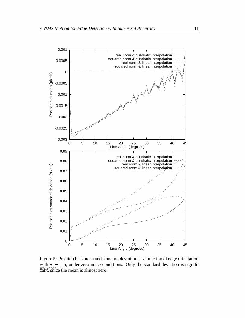
4.3 Edge position

The mean and standard deviation of the position bias for the different sub-pixel edgedetection methods are presented in Figure 5. The mean of the position bias is close tozero for straight edges (less than 1

200pixel in any case). The Gaussian derivative filter

used for preprocessing had a � of 1:5, this is a typical value to use with real images.For the classic NMS method, the maximum standard deviation of the position biasis 0:40 pixels at 440, far over the sub-pixel methods. We can see with this figure thatthe best method for sub-pixel edge detection is to use the real gradient norm as inputand to estimate the gradient norm in the direction of the gradient using quadraticinterpolation between the three neighboring points in the direction of the gradient.For a smaller computational cost, using the squared gradient norm with quadraticinterpolation or the real norm with linear interpolation give rather good estimates.

INRIA


-0.003

-0.0025

-0.002

-0.0015

-0.001

-0.0005

0

0.0005

0.001

0 5 10 15 20 25 30 35 40 45

Pos

ition

bia

s m

ean

(pix

els)

Line Angle (degrees)

real norm & quadratic interpolationsquared norm & quadratic interpolation

real norm & linear interpolationsquared norm & linear interpolation

0

0.01

0.02

0.03

0.04

0.05

0.06

0.07

0.08

0.09

0 5 10 15 20 25 30 35 40 45

Pos

ition

bia

s st

anda

rd d

evia

tion

(pix

els)




Figure 5: Position bias mean and standard deviation as a function of edge orientationwith � = 1:5, under zero-noise conditions. Only the standard deviation is signifi-cant, since the mean is almost zero.RR n˚2724


We tested the robustness of the best method (real norm and quadratic approxi-mation) by applying Gaussian noise to the image intensity for 512 � 512 images.The standard deviation of the edge position bias was calculated for different valuesof the intensity noise standard deviation and the Gaussian derivative filter standarddeviation �. As shown in Figure 6, � = 1:5 gives the best results when there is notmuch noise but when the noise standard deviation is more than 40 the edge is almostalways cut, so that bigger values of � should be used. The same thing happens for� = 2:5 when noise is more than 65. All these results are comparable in accuracywith those of Nalwa and Binford (compare those results with figures 10 and 11 of[12]), though this method is a lot faster and simpler.

4.4 Edge orientation

To prove that this edge detector gives excellent results we calculated the edge ori-entation in a very simple way, as the orientation of the line joining two consecutiveedge points. This gives good results under zero noise conditions (Figure 7), but whenthere is noise in image intensity or when one needs more precision, smoothing theimage intensity or using regularization gives better results. Figure 7 also shows thatthe edge orientation mean is slightly biased when using this method. This bias isdue to the way edge pixels are distributed along the edge: the distance between twoedge pixels may vary between 0 and 1 pixel, and this distance is correlated with theorientation of the line joining these two pixels. These figures can be compared withfigures 8.12 and 8.13 in [9].

To calculate a better value of the edge orientation we could use some kind of reg-ularization on the data, like for example calculate a least squares approximation of nconsecutive points by a line or a higher order curve. This would reduce significantlyboth the standard deviation of the measures and the angle bias we noticed before, butthe local character of the measure would be lost if the data is too much regularized.

Since the computation of edge orientation was just used as a simple example toillustrate the accuracy of this edge detection process, we will not develop further thediscussion on how to compute edge orientation in a good way.

INRIA


0

0.2

0.4

0.6

0.8

1

0 20 40 60 80 100

Pos

ition

est

imat

ed s

tand

ard

devi

atio

n (p

ixel

s)

Image noise standard deviation

sigma = 1.5sigma = 2.5sigma = 4.0

0

2

4

6

8

10

0 20 40 60 80 100

Ang

le e

stim

ated

sta

ndar

d de

viat

ion

(deg

rees

)

Image noise standard deviation

sigma = 1.5sigma = 2.5sigma = 4.0

Figure 6: Position and angle bias standard deviation as a function of image noisestandard deviation for different values of the smoothing parameter �. Edge Orien-tation is 22:50 and edge contrast is 100.RR n˚2724


-0.2

0

0.2

0.4

0.6

0.8

1

1.2

1.4

0 5 10 15 20 25 30 35 40 45

Ang

le b

ias

mea

n (d

egre

es)




0

2

4

6

8

10

12

14

0 5 10 15 20 25 30 35 40 45

Ang

le b

ias

stan

dard

dev

iatio

n (d

egre

es)




Figure 7: Angle bias mean and standard deviation as a function of edge orientationwith � = 1:5. The angle is calculated using the line joining two consecutive edgepixels (the distance between two consecutive edge pixels is less than 1 pixel).INRIA


4.5 Other results

For the best configuration of the edge detection process (i.e. use the real norm andquadratic interpolation between neighbors for the NMS), we calculated the edge po-sition bias and orientation bias mean and standard deviation (Figure 8) on the circleimages. We can see that the edge position is always found inside the circle. Thisbehavior is normal and not due to the edge detection method, as it comes from theGaussian filtering, as shown in [1], and any smoothing operator will give the samekind of results. We compared the measured displacement with the theoretical dis-placement [1] and the two curves fit perfectly. The only way to avoid this error isto have a model that not only takes into account the image intensity smoothing [12],but also the local curvature or a more general shape (like a corner shape in [7]).

We can also notice that the angle bias mean and standard deviation are lower thanthose that were found for straight edges. This is maybe due to the fact that straightedges generate more “bad” situations than curves.

We present results on part of a real aerial image (Figure 9) of both the classicmethod and our method. We can easily see that the shape of curved features that wasalmost lost with the classic method is still present with our method. The brain image(Figure 10) is another example of the precision of our edge detection method. Theseimages were taken from the database created at the SPIE Conference “Applicationof Artificial Intelligence X: Machine Vision and Robotics”.

5 Conclusion

In this article we presented an enhancement of the Non-Maxima Suppression edgedetection method which gives us the edge position at a sub-pixel accuracy. Sincethis method is very simple and costs only a few additions and multiplications perdetected edge pixel, it can be easily implemented and incorporated in a real-timevision system, and it should be used to increase the precision and reliability of visionalgorithms that use edges as input.

The result we got on a wide variety of synthetic and real images are very promis-ing since they show that the precision of this edge detector is less than 1

10of a pixel.

We computed the accuracy of this edge detection method in an objective manner, sothat the results can be easily compared with other algorithms.

RR n˚2724


-0.45

-0.4

-0.35

-0.3

-0.25

-0.2

-0.15

-0.1

-0.05

0

5 10 15 20 25 30 35 40 45 50

Pos

ition

bia

s m

ean

and

stan

dard

dev

iatio

n (p

ixel

s)

Circle radius (pixels)

real norm & quadratic interpolation

-0.2

0

0.2

0.4

0.6

0.8

1

1.2

1.4

1.6

1.8

2

0 5 10 15 20 25 30 35 40 45 50

Ang

le b

ias

mea

n an

d st

anda

rd d

evia

tion

(deg

rees

)

Circle radius (pixels)

angle bias meanangle bias standard deviation

Figure 8: Measured edge displacement as a function of circle radius, and angle biasmean and standard deviation. We used a Gaussian filter with � = 2:0 to calculatederivatives. The displacement in the case of curved edges is not due to the edge de-tection method (it is due to image smoothing), and corresponds to what is predictedby the theory [1].

INRIA


Figure 9: Results of the classic NMS algorithm (left) and of the sub-pixel approxi-mation (right) on a 100x100 region of an aerial image. The gradient was calculatedusing a second order Deriche recursive filter with � = 1:2.

RR n˚2724


Figure 10: Result of the edge detection at sub-pixel accuracy on a 175�175magneticresonance image of a human brain.

INRIA


One advantage over existing edge refinement methods [11, 14, 15, 12] is its verylow computational cost, since we only do a one-dimensional interpolation wheremost other methods work on two-dimensional data. Besides, other methods usuallytry to find a better estimate of the edge position using edge pixels that are given up towithin a pixel, thus using regularization, whereas this method gets a better estimateof the edge position directly from the image intensity data.

In the future, we plan to use this edge detector to calculate some higher degreedifferential properties of the curves such as Euclidean, affine, or even projective cur-vature, and we will also use it to enhance the precision of existing and future algo-rithms.

References

[1] V. Berzins. Accuracy of laplacian edge detectors. Computer Vision, Graphics,and Image Processing, 27:195–210, 1984.

[2] J. F. Canny. Finding edges and lines in images. Technical Report AI-TR-720,Massachusets Institute of Technology, Artificial Intelligence Laboratory, June1983.

[3] J. F. Canny. A computational approach to edge detection. IEEE Transactionson Pattern Analysis and Machine Intelligence, 8(6):769–798, November 1986.

[4] R. Deriche. Using canny’s criteria to derive a recursively implemented optimaledge detector. The International Journal of Computer Vision, 1(2):167–187,May 1987.

[5] R. Deriche. Fast algorithms for low-level vision. IEEE Transactions on PatternAnalysis and Machine Intelligence, 1(12):78–88, January 1990.

[6] R. Deriche. Recursively implementing the gaussian and its derivatives. Tech-nical Report 1893, INRIA, Unite de Recherche Sophia-Antipolis, 1993.

[7] R. Deriche and T. Blaszka. Recovering and characterizing image features usingan efficient model based approach. In Proceedings of the International Confer-ence on Computer Vision and Pattern Recognition, pages 530–535, New-York,June 1993. IEEE Computer Society, IEEE.

RR n˚2724


[8] O. D. Faugeras. Geometrie affine et projective en vision par ordinateur : I lecas des courbes. Technical report, INRIA, 1993. To appear.

[9] R. M. Haralick and L. G. Shapiro. Computer and Robot Vision, volume 1.Addison-Wesley, 1992.

[10] Robert Haralick. Digital step edges from zero crossing of second directionalderivatives. IEEE Transactions on Pattern Analysis and Machine Intelligence,6(1):58–68, January 1984.

[11] A. Huertas and G. Medioni. Detection of intensity changes with subpixel accu-racy using laplacian-gaussian masks. IEEE Transactions on Pattern Analysisand Machine Intelligence, 8(5):651–664, September 1986.

[12] V. S. Nalwa and T. O. Binford. On detecting edges. IEEE Transactions onPattern Analysis and Machine Intelligence, 8(6):699–714, 1986.

[13] Jun Shen and Serge Castan. An optimal linear operator for step edge detection.CVGIP: Graphics Models and Image Processing, 54(2):112–133, March 1992.

[14] Ali J. Tababai and O. Robert Mitchell. Edge location to subpixel values in digi-tal imagery. IEEE Transactions on Pattern Analysis and Machine Intelligence,6(2):188–201, March 1984.

[15] Thierry Vieville and Olivier D. Faugeras. Robust and fast computation of unbi-ased intensity derivatives in images. In Giulio Sandini, editor, Proceedings ofthe 2nd ECCV, pages 203–211, Santa-Margherita, Italy, 1992. Springer-Verlag.

INRIA

Unite de recherche INRIA Lorraine, Technopole de Nancy-Brabois, Campus scientifique,615 rue du Jardin Botanique, BP 101, 54600 VILLERS LES NANCY

Unite de recherche INRIA Rennes, Irisa, Campus universitaire de Beaulieu, 35042 RENNES CedexUnite de recherche INRIA Rhone-Alpes, 46 avenue Felix Viallet, 38031 GRENOBLE Cedex 1

Unite de recherche INRIA Rocquencourt, Domaine de Voluceau, Rocquencourt, BP 105, 78153 LE CHESNAY CedexUnite de recherche INRIA Sophia-Antipolis, 2004 route des Lucioles, BP 93, 06902 SOPHIA-ANTIPOLIS Cedex

Editeur

INRIA, Domaine de Voluceau, Rocquencourt, BP 105, 78153 LE CHESNAY Cedex (France)

ISSN 0249-6399

Documents

A Non-Maxima Suppression Method for Edge Detection …dev.ipol.im/~morel/Dossier_MVA_2011_Cours_Transparents_Documen… · ISSN 0249-6399 apport de recherche INSTITUT NATIONAL DE