A Non-preemptive Scheduling Algorithm for Soft Real-time Systems

Wenming Li, Krishna Kavi1 and Robert Akl The University of North Texas

1 Please direct all correspondence to Krishna Kavi, Department of Computer Science and Engineering, The University of North Texas,

P.O. Box 311366, Denton, Texas 76203, kavi@cse.unt.edu

Abstract

Real-time systems are often designed using preemp-tive scheduling and worst-case execution time esti-mates to guarantee the execution of high priority tasks. There is, however, an interest in exploring non-preemptive scheduling models for real-time systems, particularly for soft real-time multimedia applications. In this paper, we propose a new algorithm that uses multiple scheduling strategies for efficient non-preemptive scheduling of tasks. Our goal is to improve the success ratio of the well-known Earliest Deadline First (EDF) approach when the load on the system is very high and to improve the overall performance in both underloaded and overloaded conditions. Our approach, known as group-EDF (gEDF) is based on dynamic grouping of tasks with deadlines that are very close to each other, and using Shortest Job First (SJF) technique to schedule tasks within the group. We will present results comparing gEDF with other real-time algorithms including, EDF, Best-effort, and Guaran-tee, by using randomly generated tasks with varying execution times, release times, deadlines and tolerance to missing deadlines, under varying workloads. We believe that grouping tasks dynamically with similar deadlines and utilizing a secondary criteria, such as minimizing the total execution time (or other metrics such as power or resource availability that can be easily extended) for scheduling tasks within a group, can lead to new and more efficient real-time schedul-ing algorithms. Keywords: Soft Real-time Systems, Non-preemptive Real-time Scheduling, Earliest Deadline First (EDF), Shortest Job First (SJF), Best-Effort Scheduling, Group EDF. 1. Introduction

The Earliest Deadline First (EDF) algorithm is the most widely studied scheduling algorithm for real-time systems [i]. For a set of preemptive tasks (be they periodic, aperiodic, or sporadic), EDF will find a schedule if a schedule is possible [ii]. The application of EDF for non-preemptive tasks is not as widely investigated. It is our contention that non-preemptive scheduling is more efficient, particularly for soft real-time applications and applications de-signed for multithreaded systems, than the preemp-

tive approach since the non-preemptive model reduc-es the overhead needed for switching among tasks (or threads) [iii, iv]. EDF is optimal for sporadic non-preemptive tasks, but EDF may not find an optimal schedule for periodic and aperiodic non-preemptive tasks. It has been shown that scheduling periodic and aperiodic non-preemptive tasks is NP-hard [v, vi , vii]. However, non-preemptive EDF techniques have produced near optimal schedules for periodic and aperiodic tasks, particularly when the system is light-ly loaded. When the system is overloaded, however, it has been shown that the EDF approach leads to very poor performance (low success rates) [viii]. In this paper, a system load or utilization is used to refer to the sum of the execution times of pending tasks as related to the time available to complete the tasks. The poor performance of EDF is due to the fact that, as tasks that are scheduled based on their deadlines miss their deadlines, other tasks waiting for their turn are likely to miss their deadlines also – an outcome sometimes known as the domino effect. It should also be remembered that Worst Case Execution Time (WCET) estimates for tasks are used in most real-time systems. We believe that, in practice, WCET estimates are very conservative, and more aggressive scheduling schemes based on average execution times for soft real-time systems using either EDF or hybrid algorithms can lead to higher performance.

While investigating scheduling algorithms, we have analyzed a variation of EDF that can improve success ratios (that is, the number of tasks that have been successfully scheduled to meet their deadlines), particularly in overloaded conditions. The new algo-rithm can also decrease the average response time for tasks. We call our algorithm group-EDF, or gEDF, where the tasks with “similar” deadlines are grouped together (i.e., deadlines that are very close to one another), and the Shortest Job First (SJF) algorithm is used for scheduling tasks within a group. It should be noted that our approach is different from adaptive schemes that switch between different scheduling strategies based on system load; gEDF is used in overloaded as well as underloaded conditions. The computational complexity of gEDF is the same as that of EDF. In this paper, we will evaluate the per-formance of gEDF using randomly generated tasks with varying execution times, release times, dead-

lines and tolerance to missing deadlines, under vary-ing loads.

We believe that gEDF is particularly useful for soft real-time systems as well as applications known as “anytime algorithms” and “approximate algo-rithms,” where applications generate more accurate results or rewards with increased execution times [ix, x]. Examples of such applications include search algorithms, neural-net based learning in AI, FFT and block-recursive filters used for audio and image pro-cessing. We model such applications using a toler-ance parameter that describes by how much a task can miss its deadline, or by how much the task’s execution time can be truncated when the deadline is approaching.

This paper is organized as follows. In section 2, we present related work. In section 3, we present our real-time system model. Numerical results are pre-sented in section 4. Conclusions are given in section 5.

2. Related Work

The EDF algorithm schedules real-time tasks based on their deadlines. Because of its optimality for periodic, aperiodic, and sporadic preemptive tasks, its optimality for sporadic non-preemptive tasks, and its acceptable performance for periodic and aperiodic non-preemptive tasks, EDF is widely studied as a dynamic priority-driven scheduling scheme [v]. EDF is more efficient than many other scheduling algo-rithms, including the static Rate-Monotonic schedul-ing algorithm. For preemptive tasks, EDF is able to reach the maximum possible processor utilization when lightly loaded. Although finding an optimal schedule for periodic and aperiodic non-preemptive tasks is NP-hard [vi, vii], our experiments have shown that EDF can achieve very good results even for non-preemptive tasks when the system is lightly loaded. However, when the processor is over-loaded (i.e., the combined requirements of pending tasks exceed the capabilities of the system) EDF performs poorly. Researchers have proposed several adaptive techniques for handling heavily loaded situations, but they require the detection of the overload condition.

A Best-effort algorithm [viii] is based on the as-sumption that the probability of a high value-density task arriving is low. The value-density is defined by V/C, where V is the value of a task and C is its worst-case execution time. Given a set of tasks with defined values for successful completion, it can be shown that a sequence of tasks in decreasing order by value-density will produce the maximum value as com-pared to any other scheduling technique. The Best-effort algorithm admits tasks based on their value-densities and schedules them using the EDF policy. When higher value tasks are admitted, some lower

value tasks may be deleted from the schedule or de-layed until no other tasks with higher value exist. One key consideration in implementing such a policy is the estimation of current workload, which is either very difficult or very inaccurate in most practical systems that utilize WCET estimations. WCET esti-mation requires complex analysis of tasks [xi, xii], and, in most cases, the estimates are significantly larger than average execution times of tasks. Thus the Best-effort algorithms that use WCET to estimate loads may lead to sub-optimal value realization. Best-effort has been used as an overload control strategy for EDF.

Other approaches for detecting overload and re-jecting tasks were reported in [xiii, xiv]. In the Guar-antee scheme [xiii], the load on the processor is con-trolled by performing acceptance tests on new tasks entering the system. If the new task is found sched-ulable under worst-case assumptions, it is accepted; otherwise, the arriving task is rejected. In the Robust scheme [xiv], the acceptance test is based on EDF; if overloaded, one or more tasks may be rejected based on their importance. Because the Guarantee and Ro-bust algorithms also rely on computing the schedules of tasks, often based on worst-case estimates, they usually lead to underutilization of resources. Thus Best-effort, Guarantee, or Robust scheduling algo-rithms are not good for soft real-time systems or applications that are generally referred to as “any-time” or “approximate” algorithms [x].

The combination of SJF and EDF, referred to as SCAN-EDF for disk scheduling, was proposed in [xv]. In the algorithm, SJF is only used to break a tie between tasks with identical deadlines. The work in [xvi , xvii ] is very closely related to our idea of groups. This approach quantizes deadlines into dead-line bins and places tasks into these bins. However, tasks within a bin (or group) are scheduled using First Come First Served (FCFS). The gEDF groups that we use are created dynamically instead of stati-cally as done in [16,17].

One integrated real-time scheduler including Best-effort strategy for general-purpose operating systems has been proposed in [xviii]. However, this approach relies on the preemptive scheduling and uses Best-effort as an overload control strategy. 3. Real-time System Model 3.1 Definitions

A job τi in a real-time system or a thread in multithreading processing is defined as τi = (ri, ei, Di, Pi); where ri is its release time (or its arrival time ); ei is either its predicted worst-case or average execution time; Di is its deadline. We also maintain a dynamic deadline di = ri + Di , which tracks the absolute time before the deadline expires. If modeling periodic

jobs, Pi defines a task’s periodicity. Note that aperi-odic and sporadic jobs can be modeled by setting Pi appropriately.

For the experiments, we generated a fixed num-ber (N) of jobs with varying arrivals, execution times and deadlines. We assume that the jobs are mutually independent. Each experiment terminated when the predetermined experimental time T expired. This permitted us to investigate the sensitivity of the vari-ous task parameters on the success rates of EDF and gEDF. We use random distributions available in MATLAB to generate the necessary parameters with tasks.

A group in the gEDF algorithm depends on a group range parameter Gr. τj belongs to the same group as τi if di ≤ dj ≤ (di + Gr*(di – t))2, where t is the current time, 1 ≤ i, j ≤ N. In other words, we group jobs with very close deadlines together. We schedule groups based on EDF (all jobs in a group with an earlier deadline will be considered for sched-uling before jobs in a group with later deadlines), but schedule jobs within a group using shortest job first (SJF) approach. Since SJF results in more (albeit shorter) jobs completing, intuitively gEDF should lead to a higher success rate than pure EDF. We use the following notations for various pa-rameters and computed values: ρ: is the utilization of the system, ρ = Σei / T. This is

also called the load. γ: is the success ratio, γ = the number of jobs complet-

ed successfully / N. Tr: is the deadline tolerance for soft real-time systems.

A job τ is schedulable if τ finishes before the time (1 + Tr) * D, where Tr ≥ 0.

µe: is used either as the average execution time or the worst case execution time, and defines the ex-pected value of the exponential distribution used for this purpose.

µr: is used to generate arrival times of jobs, and is the expected value of the exponential distribution used for this purpose.

µD: is the expected value of the random distribution used to generate task deadlines. We set this pa-rameter as a multiple of µe.

ℜ: is the average response time of the jobs. ∂: is the response-time ratio, ∂ = ℜ / µe. ηγ: is the success-ratio performance factor, ηγ = γgEDF /

γEDF. This is used to compare gEDF with EDF. η∂: is the response-time performance factor, η∂ = ∂EDF

/ ∂gEDF. This is used to compare gEDF with EDF. 3.2 gEDF Algorithm

2 We are using the remaining time to a task deadline (called

dynamic deadlines) in forming groups. We found that using static deadlines for defining groups did not signifi-cantly change the results.

We assume a uniprocessor system. QgEDF is a queue for gEDF scheduling. The current time is rep-resented as t. |Q| represents the length of the queue Q. τ = (r, e, D, P) yields the job at the head of the queue. We define groups in gEDF as follows: gEDF Group = {τk | τk ∈ QgEDF, dk – d1 ≤ D1 * Gr, 1 ≤ k ≤ m, where m ≤ |QgEDF|}, where, D1 is the deadline of the first job in a group. Algorithm:

1. Enqueue(QgEDF, τ) if ( τ’s deadline d > t ) insert job τ into QgEDF by Earliest Dead-

lineFirst, i.e. di ≤ di+1 ≤ di+2, where τi, τi+1, τi+2 ∈ QgEDF, 1 ≤ i ≤ |QgEDF| - 2; end 2. τmin = Dequeue (QgEDF) if QgEDF ≠ φ find a job τmin with emin = min {ek | τk ∈ QgEDF, dk – d1 ≤ Gr*D1, 1 ≤ k ≤ m, where m ≤ |QgEDF|}; run it and delete τmin from QgEDF; end

Enqueue is invoked on job arrivals and Dequeue is called when the processor becomes idle. The algo-rithm that we presented tends to favor smaller jobs and thus it does not always guarantee fairness. Also the algorithm needs to sort the jobs in each group, which could incur more overhead during execution than EDF. However, in most practical systems, the number of jobs in a group is small and the added runtime overhead will be negligible. 4. Numerical Results

MATLAB is used to generate tasks and the gen-erated tasks are scheduled using EDF, gEDF, or other scheduling algorithms. For each chosen set of param-eters, we have repeated each experiment 100 times (each time, generated N tasks using the random prob-ability distributions and scheduled the generated tasks) and computed the average success rate. In what follows, we report the results and analyze the sensi-tivity of gEDF to the various parameters used in the experiments, the effects of the percentage of small jobs, and how well gEDF performs when compared to Best-Effort algorithm. Note that we use the non-preemptive task model.

4.1 Comparison of gEDF and EDF

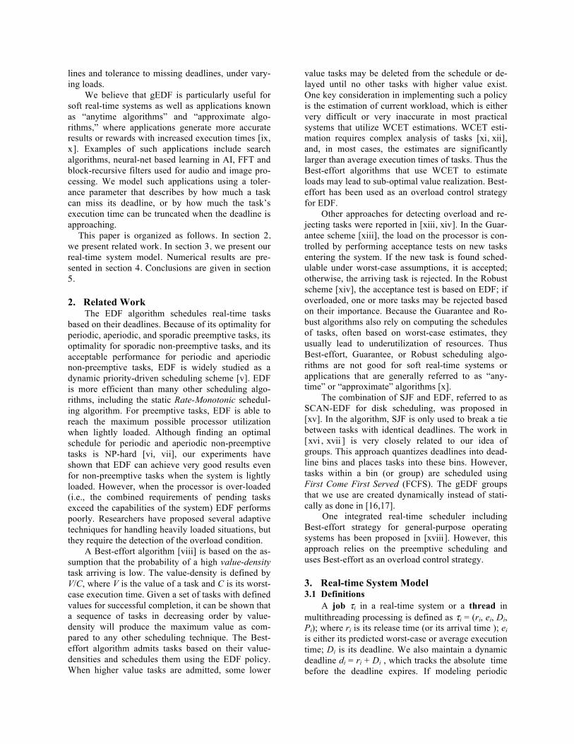
4.1.1 Experiment 1 – Effect of Deadline Tolerance Figures 1-3 show that gEDF achieves higher

success rate than EDF when the deadline tolerance (i.e., soft real-time nature of the jobs) is varied from 20%, 50% to 100% (that is, a task can miss its dead-line by 20%, 50% and 100%).

0.65

0.70

0.75

0.80

0.85

0.90

0.95

1.00

0.1

0.3

0.5

0.7

0.9

1.1

1.3

1.5

1.7

1.9

2.1

2.3

2.5

2.7

2.9

Utilization

Suc

cess

Rat

io

EDF: Tr=0.2

gEDF: Tr=0.2

Figure 1: Success rates when deadline tolerance is 0.2.

For these experiments, we generated tasks by

fixing expected execution rate and deadline parame-ters of the probability distributions, but varied arrival rate parameter to change the system load. The group range for these experiments is fixed at Gr = 0.4 (i.e., all jobs whose deadlines fall within 40% of the dead-line of current job are in the same group). It should be noted that gEDF’s success rates are consistently as good as those of EDF under light loads (utilization is less than 1), but higher than those of EDF under heavy loads (utilization is greater than 1, see the X-axis). Both EDF and gEDF achieve higher success rates when tasks are provided with greater deadline tolerance. The tolerance benefits gEDF more than EDF, particularly under heavy loads. Thus, gEDF is better suited for soft real-time tasks.

0.50

0.60

0.70

0.80

0.90

1.00

0.1

0.3

0.5

0.7

0.9

1.1

1.3

1.5

1.7

1.9

2.1

2.3

2.5

2.7

2.9

Utilization

Suc

cess

Rat

io

EDF: Tr=0.5

gEDF: Tr=0.5

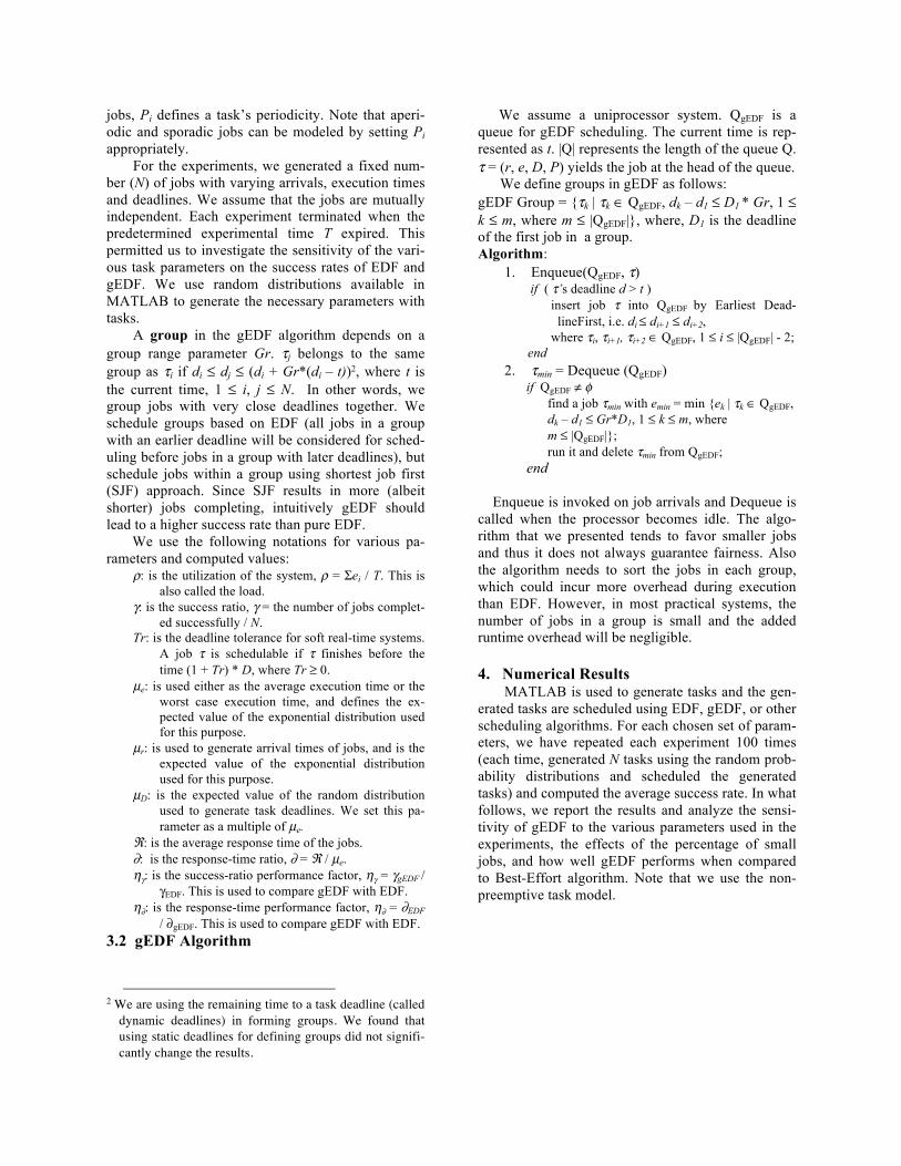
Figure 2: Success rates when deadline tolerance is 0.5.

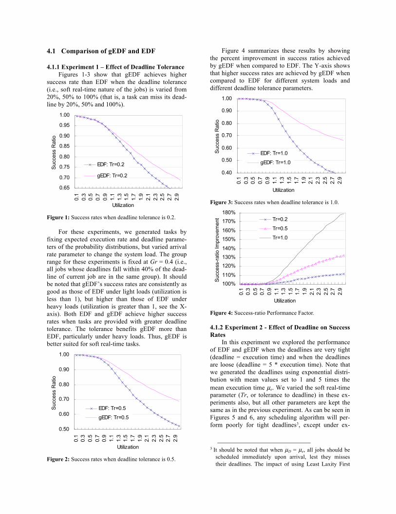
Figure 4 summarizes these results by showing the percent improvement in success ratios achieved by gEDF when compared to EDF. The Y-axis shows that higher success rates are achieved by gEDF when compared to EDF for different system loads and different deadline tolerance parameters.

0.40

0.50

0.60

0.70

0.80

0.90

1.00

0.1

0.3

0.5

0.7

0.9

1.1

1.3

1.5

1.7

1.9

2.1

2.3

2.5

2.7

2.9

Utilization

Suc

cess

Rat

io

EDF: Tr=1.0

gEDF: Tr=1.0

Figure 3: Success rates when deadline tolerance is 1.0.

100%

110%

120%

130%

140%

150%

160%

170%

180%

0.1

0.3

0.5

0.7

0.9

1.1

1.3

1.5

1.7

1.9

2.1

2.3

2.5

2.7

2.9

Utilization

Suc

cess

-rat

io Im

prov

emen

t Tr=0.2

Tr=0.5

Tr=1.0

Figure 4: Success-ratio Performance Factor.

4.1.2 Experiment 2 - Effect of Deadline on Success Rates

In this experiment we explored the performance of EDF and gEDF when the deadlines are very tight (deadline = execution time) and when the deadlines are loose (deadline = 5 * execution time). Note that we generated the deadlines using exponential distri-bution with mean values set to 1 and 5 times the mean execution time µe. We varied the soft real-time parameter (Tr, or tolerance to deadline) in these ex-periments also, but all other parameters are kept the same as in the previous experiment. As can be seen in Figures 5 and 6, any scheduling algorithm will per-form poorly for tight deadlines3, except under ex-

3 It should be noted that when µD = µe, all jobs should be

scheduled immediately upon arrival, lest they misses their deadlines. The impact of using Least Laxity First

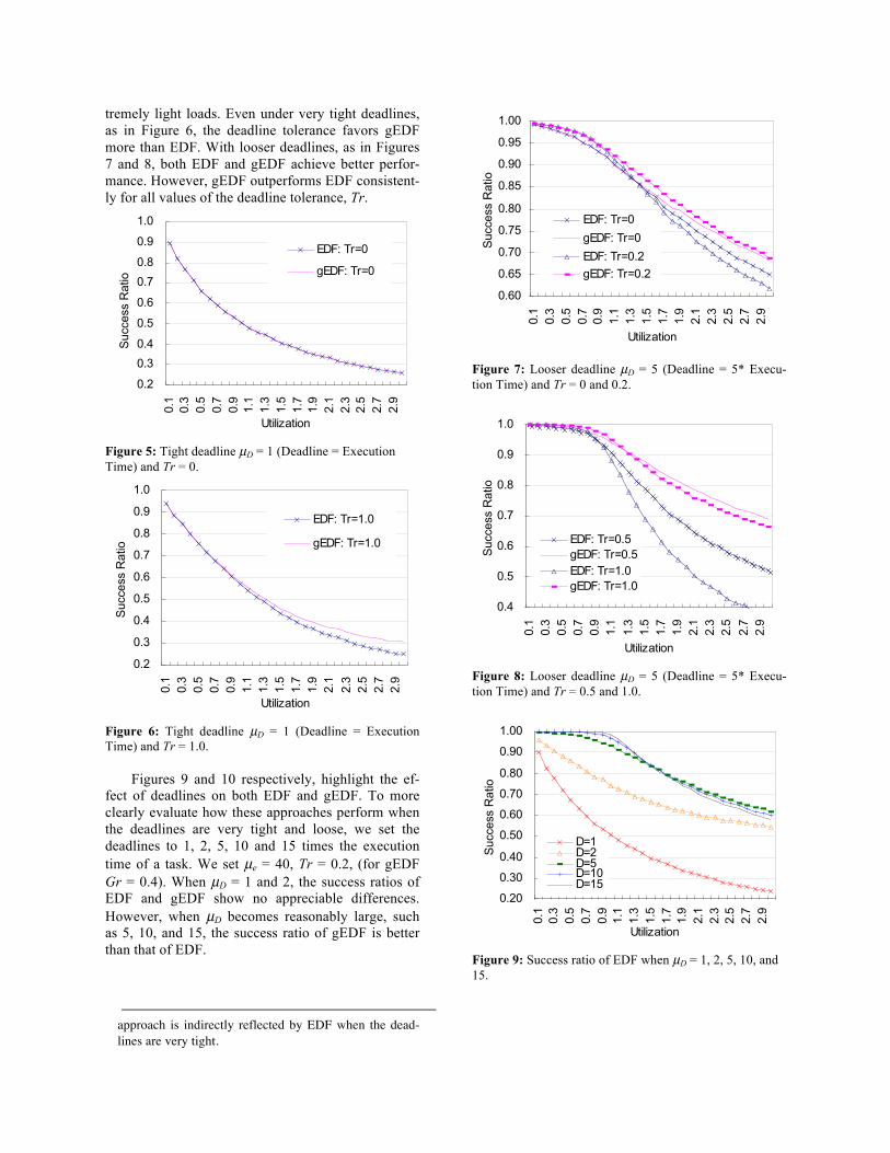
tremely light loads. Even under very tight deadlines, as in Figure 6, the deadline tolerance favors gEDF more than EDF. With looser deadlines, as in Figures 7 and 8, both EDF and gEDF achieve better perfor-mance. However, gEDF outperforms EDF consistent-ly for all values of the deadline tolerance, Tr.

0.2

0.3

0.4

0.5

0.6

0.7

0.8

0.9

1.0

0.1

0.3

0.5

0.7

0.9

1.1

1.3

1.5

1.7

1.9

2.1

2.3

2.5

2.7

2.9

Utilization

Suc

cess

Rat

io

EDF: Tr=0

gEDF: Tr=0

Figure 5: Tight deadline µD = 1 (Deadline = Execution Time) and Tr = 0.

0.2

0.3

0.4

0.5

0.6

0.7

0.8

0.9

1.0

0.1

0.3

0.5

0.7

0.9

1.1

1.3

1.5

1.7

1.9

2.1

2.3

2.5

2.7

2.9

Utilization

Suc

cess

Rat

io

EDF: Tr=1.0

gEDF: Tr=1.0

Figure 6: Tight deadline µD = 1 (Deadline = Execution Time) and Tr = 1.0.

Figures 9 and 10 respectively, highlight the ef-

fect of deadlines on both EDF and gEDF. To more clearly evaluate how these approaches perform when the deadlines are very tight and loose, we set the deadlines to 1, 2, 5, 10 and 15 times the execution time of a task. We set µe = 40, Tr = 0.2, (for gEDF Gr = 0.4). When µD = 1 and 2, the success ratios of EDF and gEDF show no appreciable differences. However, when µD becomes reasonably large, such as 5, 10, and 15, the success ratio of gEDF is better than that of EDF.

approach is indirectly reflected by EDF when the dead-lines are very tight.

0.60

0.65

0.70

0.75

0.80

0.85

0.90

0.95

1.00

0.1

0.3

0.5

0.7

0.9

1.1

1.3

1.5

1.7

1.9

2.1

2.3

2.5

2.7

2.9

Utilization

Suc

cess

Rat

io

EDF: Tr=0gEDF: Tr=0EDF: Tr=0.2gEDF: Tr=0.2

Figure 7: Looser deadline µD = 5 (Deadline = 5* Execu-tion Time) and Tr = 0 and 0.2.

0.4

0.5

0.6

0.7

0.8

0.9

1.0

0.1

0.3

0.5

0.7

0.9

1.1

1.3

1.5

1.7

1.9

2.1

2.3

2.5

2.7

2.9

Utilization

Suc

cess

Rat

io

EDF: Tr=0.5gEDF: Tr=0.5EDF: Tr=1.0gEDF: Tr=1.0

Figure 8: Looser deadline µD = 5 (Deadline = 5* Execu-tion Time) and Tr = 0.5 and 1.0.

0.20

0.30

0.40

0.50

0.60

0.70

0.80

0.90

1.00

0.1

0.3

0.5

0.7

0.9

1.1

1.3

1.5

1.7

1.9

2.1

2.3

2.5

2.7

2.9

Utilization

Suc

cess

Rat

io

D=1D=2D=5D=10D=15

Figure 9: Success ratio of EDF when µD = 1, 2, 5, 10, and 15.

0.20

0.30

0.40

0.50

0.60

0.70

0.80

0.90

1.00

0.1

0.3

0.5

0.7

0.9

1.1

1.3

1.5

1.7

1.9

2.1

2.3

2.5

2.7

2.9

Utilization

Suc

cess

Rat

io

D=1D=2D=5D=10D=15

Figure 10: Success ratio of gEDF when µD = 1, 2, 5, 10, and 15.

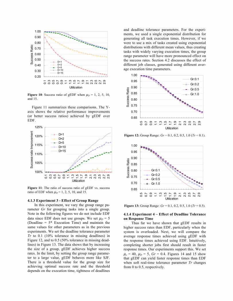
Figure 11 summarizes these comparisons. The Y-axis shows the relative performance improvements (or better success ratios) achieved by gEDF over EDF.

100%

105%

110%

115%

120%

125%

0.1

0.3

0.5

0.7

0.9

1.1

1.3

1.5

1.7

1.9

2.1

2.3

2.5

2.7

2.9

Utilization

Suc

cess

-rat

io Im

prov

emen

t

D=1D=2D=5D=10D=15

Figure 11: The ratio of success ratio of gEDF vs. success ratio of EDF when µD = 1, 2, 5, 10, and 15. 4.1.3 Experiment 3 - Effect of Group Range

In this experiment, we vary the group range pa-rameter Gr for grouping tasks into a single group. Note in the following figures we do not include EDF data since EDF does not use groups. We set µD = 5 (Deadline = 5* Execution Time) and maintain the same values for other parameters as in the previous experiments. We set the deadline tolerance parameter Tr to 0.1 (10% tolerance in missing deadlines) in Figure 12, and to 0.5 (50% tolerance in missing dead-lines) in Figure 13. The data shows that by increasing the size of a group, gEDF achieves higher success rates. In the limit, by setting the group range parame-ter to a large value, gEDF behaves more like SJF. There is a threshold value for the group size for achieving optimal success rate and the threshold depends on the execution time, tightness of deadlines

and deadline tolerance parameters. For the experi-ments, we used a single exponential distribution for generating all task execution times. However, if we were to use a mix of tasks created using exponential distributions with different mean values, thus creating tasks with widely varying execution times, the group range parameter will have more pronounced effect on the success rates. Section 4.2 discusses the effect of different job classes, generated using different aver-age execution time parameters.

0.65

0.70

0.75

0.80

0.85

0.90

0.95

1.00

0.5

0.7

0.9

1.1

1.3

1.5

1.7

1.9

2.1

2.3

2.5

2.7

2.9

UtilizationS

ucce

ss R

atio

Gr:0.1

Gr:0.2

Gr:0.5Gr:1.0

Figure 12: Group Range: Gr = 0.1, 0.2, 0.5, 1.0 (Tr = 0.1).

0.65

0.70

0.75

0.80

0.85

0.90

0.95

1.00

0.5

0.7

0.9

1.1

1.3

1.5

1.7

1.9

2.1

2.3

2.5

2.7

2.9

Utilization

Suc

cess

Rat

io

Gr:0.1Gr:0.2Gr:0.5Gr:1.0

Figure 13: Group Range: Gr = 0.1, 0.2, 0.5, 1.0 (Tr = 0.5).

4.1.4 Experiment 4 – Effect of Deadline Tolerance on Response Time

Thus far we have shown that gEDF results in higher success rates than EDF, particularly when the system is overloaded. Next, we will compare the average response times achieved using gEDF with the response times achieved using EDF. Intuitively, completing shorter jobs first should result in faster response times. Our experiments support this. We set µe = 40, µD = 5, Gr = 0.4. Figures 14 and 15 show that gEDF can yield faster response times than EDF when soft real-time tolerance parameter Tr changes from 0 to 0.5, respectively.

0

50

100

150

200

250

300

350

400

0.1

0.3

0.5

0.7

0.9

1.1

1.3

1.5

1.7

1.9

2.1

2.3

2.5

2.7

2.9

Utilization

Res

pons

e Ti

me

EDF: Tr=0

gEDF: Tr=0

Figure 14: Response time when deadline tolerance Tr = 0.

0

50

100

150

200

250

300

350

400

0.1

0.3

0.5

0.7

0.9

1.1

1.3

1.5

1.7

1.9

2.1

2.3

2.5

2.7

2.9

Utilization

Res

pons

e Ti

me

EDF: Tr=0.5

gEDF: Tr=0.5

Figure 15: Response time when deadline tolerance Tr = 0.5.

Figure 16 summarizes the improvements in re-

sponse times achieved by gEDF when compared to EDF. Note that that Y-axis shows the relative re-sponse times (and smaller number are better).

50%

60%

70%

80%

90%

100%

0.1

0.3

0.5

0.7

0.9

1.1

1.3

1.5

1.7

1.9

2.1

2.3

2.5

2.7

2.9

Utilization

Res

pons

e-tim

e Im

prov

emen

t

Tr=0Tr=0.5Tr=1.0

Figure 16: The ratio of response time of gEDF vs. re-sponse time of EDF.

4.1.5 Experiment 5 - The Effect of Tight Deadlines on Response Time

Figures 17 and 18 show the change in response time of EDF and gEDF when µD changes to 1, 2, 5, and 10. For these experiments, we set µr = µe/ρ, µe = 40, Gr = 0.4, Tr = 0.1. Like the success ratios of EDF and gEDF, when µD is 1 and 2 times µe, there is no difference between EDF and gEDF. However, when µD is larger multiple of µe, gEDF results in faster response times.

0

50

100

150

200

250

300

350

400

0.1

0.3

0.5

0.7

0.9

1.1

1.3

1.5

1.7

1.9

2.1

2.3

2.5

2.7

2.9

UtilizationR

espo

nse

Tim

e

D=1D=2D=5D=10

Figure 17: Response time of EDF when µD = 1, 2, 5, and 10.

0

50

100

150

200

250

300

350

400

0.1

0.3

0.5

0.7

0.9

1.1

1.3

1.5

1.7

1.9

2.1

2.3

2.5

2.7

2.9

Utilization

Res

pons

e Ti

me

D=1D=2D=5D=10

Figure 18: Response time of gEDF when µD = 1, 2, 5, and 10.

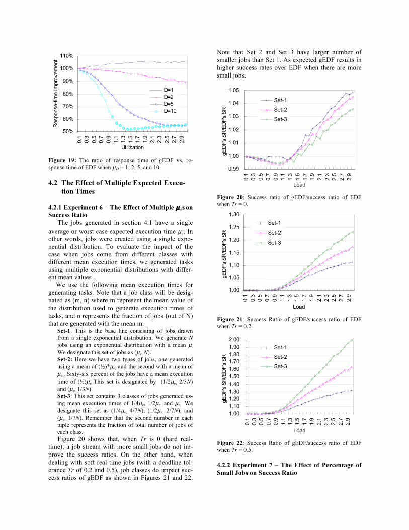
Figure 19 summarizes the improvements in re-sponse times achieved by gEDF when compared to EDF. Note that that Y-axis shows the relative re-sponse times (and smaller number are better).

50%

60%

70%

80%

90%

100%

110%

0.1

0.3

0.5

0.7

0.9

1.1

1.3

1.5

1.7

1.9

2.1

2.3

2.5

2.7

2.9

Utilization

Res

pons

e-tim

e Im

prov

emen

t

D=1D=2D=5D=10

Figure 19: The ratio of response time of gEDF vs. re-sponse time of EDF when µD = 1, 2, 5, and 10.

4.2 The Effect of Multiple Expected Execu-

tion Times 4.2.1 Experiment 6 – The Effect of Multiple µ es on Success Ratio

The jobs generated in section 4.1 have a single average or worst case expected execution time µe. In other words, jobs were created using a single expo-nential distribution. To evaluate the impact of the case when jobs come from different classes with different mean execution times, we generated tasks using multiple exponential distributions with differ-ent mean values .

We use the following mean execution times for generating tasks. Note that a job class will be desig-nated as (m, n) where m represent the mean value of the distribution used to generate execution times of tasks, and n represents the fraction of jobs (out of N) that are generated with the mean m.

Set-1: This is the base line consisting of jobs drawn from a single exponential distribution. We generate N jobs using an exponential distribution with a mean µ. We designate this set of jobs as (µe, N). Set-2: Here we have two types of jobs, one generated using a mean of (½)*µe, and the second with a mean of µe,. Sixty-six percent of the jobs have a mean execution time of (½)µe. This set is designated by (1/2µe, 2/3N) and (µe, 1/3N). Set-3: This set contains 3 classes of jobs generated us-ing mean execution times of 1/4µe, 1/2µe, and µe. We designate this set as (1/4µe, 4/7N), (1/2µe, 2/7N), and (µe, 1/7N). Remember that the second number in each tuple represents the fraction of total number of jobs of each class. Figure 20 shows that, when Tr is 0 (hard real-

time), a job stream with more small jobs do not im-prove the success ratios. On the other hand, when dealing with soft real-time jobs (with a deadline tol-erance Tr of 0.2 and 0.5), job classes do impact suc-cess ratios of gEDF as shown in Figures 21 and 22.

Note that Set 2 and Set 3 have larger number of smaller jobs than Set 1. As expected gEDF results in higher success rates over EDF when there are more small jobs.

0.99

1.00

1.01

1.02

1.03

1.04

1.05

0.1

0.3

0.5

0.7

0.9

1.1

1.3

1.5

1.7

1.9

2.1

2.3

2.5

2.7

2.9

Load

gED

F's

SR/E

DF'

s SR

Set-1

Set-2

Set-3

Figure 20: Success ratio of gEDF/success ratio of EDF when Tr = 0.

1.00

1.05

1.10

1.15

1.20

1.25

1.30

0.1

0.3

0.5

0.7

0.9

1.1

1.3

1.5

1.7

1.9

2.1

2.3

2.5

2.7

2.9

Load

gED

F's

SR/E

DF'

s SR

Set-1

Set-2

Set-3

Figure 21: Success Ratio of gEDF/success ratio of EDF when Tr = 0.2.

1.001.101.201.301.401.501.601.701.801.902.00

0.1

0.3

0.5

0.7

0.9

1.1

1.3

1.5

1.7

1.9

2.1

2.3

2.5

2.7

2.9

Load

gED

F's

SR/E

DF'

s SR

Set-1

Set-2

Set-3

Figure 22: Success Ratio of gEDF/success ratio of EDF when Tr = 0.5.

4.2.2 Experiment 7 – The Effect of Percentage of Small Jobs on Success Ratio

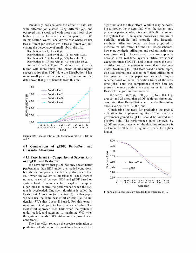
Previously, we analyzed the effect of data sets with different job classes using different µes, and observed that a workload with more small jobs show higher gEDF performance when compared to EDF. In this section, we will analyze the case where we use two different job classes (with two different µes) but change the percentage of small jobs in the mix.

Distribution 1: all jobs with µe. Distribution 2: 1/2jobs with µe; 1/2 jobs with 1/2µe. Distribution 3: 2/5jobs with µe; 3/5jobs with 1/3 µe. Distribution 4: 1/5 jobs with µe; 4/5 jobs with 1/8 µe. We set Tr = 0.5. Figure 23 shows that the distri-

bution with more small jobs, gEDF obtains higher success ratios than EDF. Note the Distribution 4 has more small jobs than any other distribution, and the data shows that gEDF benefits from this fact.

1.00

1.50

2.00

2.50

3.00

3.50

0.1

0.3

0.5

0.7

0.9

1.1

1.3

1.5

1.7

1.9

2.1

2.3

2.5

2.7

2.9

Load

gED

F's

SR/E

DF'

s SR

Distribution 1Distribution 2Distribution 3Distribution 4

Figure 23: Success ratio of gEDF/success ratio of EDF Tr = 0.5.

4.3 Comparisons of gEDF, Best-effort, and Guarantee Algorithms 4.3.1 Experiment 8 - Comparison of Success Rati-os of gEDF and Best-effort

We have shown that gEDF not only shows better performance than EDF under overloaded conditions, but shows comparable or better performance than EDF when the system is underloaded. Thus, there is no need to switch between EDF and gEDF based on system load. Researchers have explored adaptive algorithms to control the performance when the sys-tem is overloaded. One such algorithm is called the Best-effort Algorithm (see Section 2). In this paper we will use the same best effort criteria (i.e., value-density: V/C) that Locke [8] used. For this experi-ment we set all jobs to have the same value. The Best-effort approach used EDF when the system is under-loaded, and attempts to maximize V/C when the system exceeds 100% utilization (i.e., overloaded conditions).

The Best-effort relies on the precise estimation or prediction of utilization for switching between EDF

algorithm and the Best-effort. While it may be possi-ble to predict the system load when the system only processes periodic jobs, it is very difficult to compute the system load if the system processes a mixture of periodic, aperiodic, and sporadic jobs. Recently, synthetic utilization bound has been proposed to measure real utilization. For the EDF-based schemes, however, synthetic utilization and real utilization are very close [xix]. The estimated loads are imprecise because most real-time systems utilize worst-case execution times (WCET), and in most cases the actu-al utilization of the system is lower than these esti-mates. Switching to Best-Effort based on such impre-cise load estimations leads to inefficient utilization of the resources. In this paper we use a clairvoyant scheme based on actual execution times of the real-time jobs. Thus the comparisons shown here are present the most optimistic scenarios as far as the Best-Effort algorithm is concerned.

We set µr = µe/ρ, µe = 20, µD = 5, Gr = 0.4. Fig-ures 24 and 25 show that gEDF achieves higher suc-cess rates than Best-effort when the deadline toler-ance is varied, Tr = 0.2, 0.5, and 1.0.

Considering the need for predicting the precise utilization for implementing Best-Effort, any im-provements gained by gEDF should be viewed in a positive light. The performance gains achieved by gEDF are even grater when the deadline tolerance is as lenient as 50%, as in Figure 25 (even for lighter loads).

0.65

0.70

0.75

0.80

0.85

0.90

0.95

1.00

0.1

0.3

0.5

0.7

0.9

1.1

1.3

1.5

1.7

1.9

2.1

2.3

2.5

2.7

2.9

Utilization

Suc

cess

Rat

io

Best-effort

gEDF

Figure 24: Success rates when deadline tolerance is 0.2.

0.65

0.70

0.75

0.80

0.85

0.90

0.95

1.00

0.1

0.3

0.5

0.7

0.9

1.1

1.3

1.5

1.7

1.9

2.1

2.3

2.5

2.7

2.9

Utilization

Suc

cess

Rat

io

Best-effort

gEDF

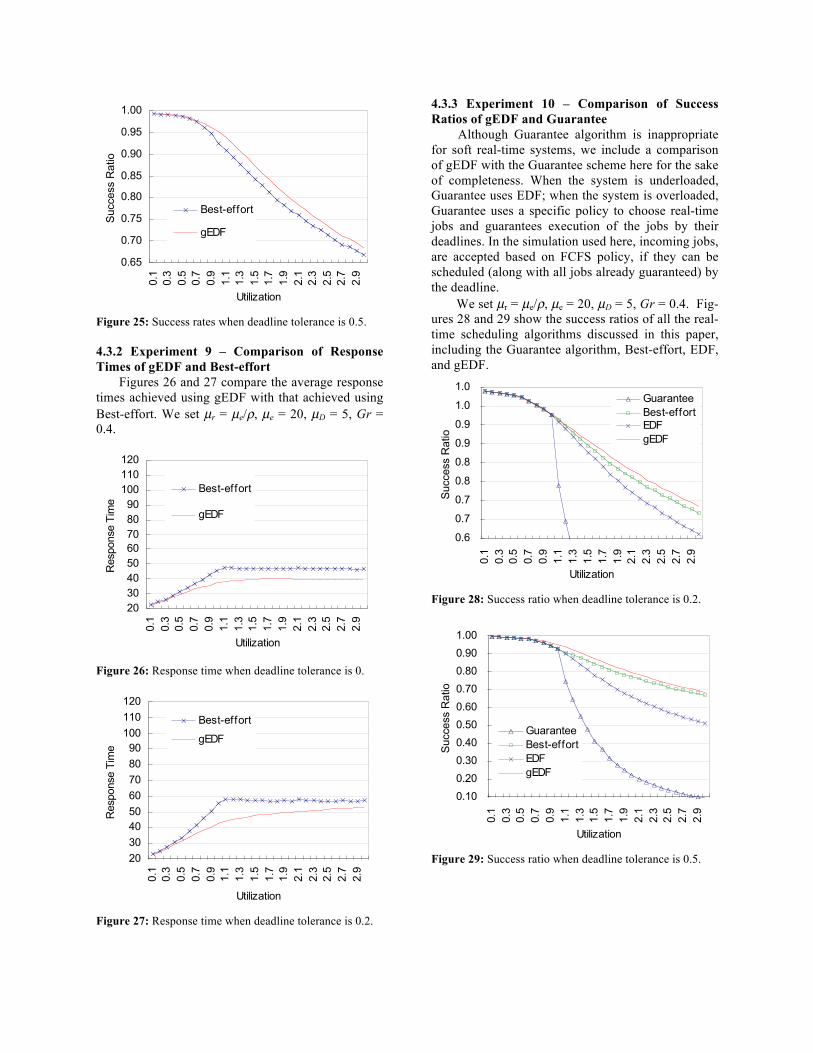
Figure 25: Success rates when deadline tolerance is 0.5. 4.3.2 Experiment 9 – Comparison of Response Times of gEDF and Best-effort

Figures 26 and 27 compare the average response times achieved using gEDF with that achieved using Best-effort. We set µr = µe/ρ, µe = 20, µD = 5, Gr = 0.4.

2030405060708090

100110120

0.1

0.3

0.5

0.7

0.9

1.1

1.3

1.5

1.7

1.9

2.1

2.3

2.5

2.7

2.9

Utilization

Res

pons

e Ti

me

Best-effort

gEDF

Figure 26: Response time when deadline tolerance is 0.

2030405060708090

100110120

0.1

0.3

0.5

0.7

0.9

1.1

1.3

1.5

1.7

1.9

2.1

2.3

2.5

2.7

2.9

Utilization

Res

pons

e Ti

me

Best-effort

gEDF

Figure 27: Response time when deadline tolerance is 0.2.

4.3.3 Experiment 10 – Comparison of Success Ratios of gEDF and Guarantee Although Guarantee algorithm is inappropriate for soft real-time systems, we include a comparison of gEDF with the Guarantee scheme here for the sake of completeness. When the system is underloaded, Guarantee uses EDF; when the system is overloaded, Guarantee uses a specific policy to choose real-time jobs and guarantees execution of the jobs by their deadlines. In the simulation used here, incoming jobs, are accepted based on FCFS policy, if they can be scheduled (along with all jobs already guaranteed) by the deadline.

We set µr = µe/ρ, µe = 20, µD = 5, Gr = 0.4. Fig-ures 28 and 29 show the success ratios of all the real-time scheduling algorithms discussed in this paper, including the Guarantee algorithm, Best-effort, EDF, and gEDF.

0.6

0.7

0.7

0.8

0.8

0.9

0.9

1.0

1.0

0.1

0.3

0.5

0.7

0.9

1.1

1.3

1.5

1.7

1.9

2.1

2.3

2.5

2.7

2.9

Utilization

Suc

cess

Rat

io

GuaranteeBest-effortEDFgEDF

Figure 28: Success ratio when deadline tolerance is 0.2.

0.10

0.20

0.30

0.40

0.50

0.60

0.70

0.80

0.90

1.00

0.1

0.3

0.5

0.7

0.9

1.1

1.3

1.5

1.7

1.9

2.1

2.3

2.5

2.7

2.9

Utilization

Suc

cess

Rat

io

GuaranteeBest-effortEDFgEDF

Figure 29: Success ratio when deadline tolerance is 0.5.

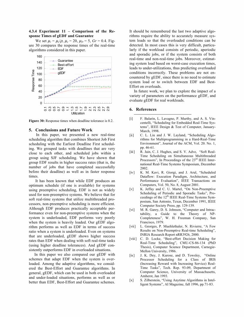
4.3.4 Experiment 11 – Comparison of the Re-sponse Times of gEDF and Guarantee

We set µr = µe/ρ, µe = 20, µD = 5, Gr = 0.4. Fig-ure 30 compares the response times of the real-time algorithms considered in this paper.

0

20

40

60

80

100

120

140

160

0.1

0.3

0.5

0.7

0.9

1.1

1.3

1.5

1.7

1.9

2.1

2.3

2.5

2.7

2.9

Utilization

Res

pons

e Ti

me

GuaranteeBest-effortEDFgEDF

Figure 30: Response times when deadline tolerance is 0.2.

5. Conclusions and Future Work

In this paper, we presented a new real-time scheduling algorithm that combines Shortest Job First scheduling with the Earliest Deadline First schedul-ing. We grouped tasks with deadlines that are very close to each other, and scheduled jobs within a group using SJF scheduling. We have shown that group EDF results in higher success rates (that is, the number of jobs that have completed successfully before their deadline) as well as in faster response times.

It has been known that while EDF produces an optimum schedule (if one is available) for systems using preemptive scheduling, EDF is not as widely used for non-preemptive systems. We believe that for soft real-time systems that utilize multithreaded pro-cessors, non-preemptive scheduling is more efficient. Although EDF produces practically acceptable per-formance even for non-preemptive systems when the system is underloaded, EDF performs very poorly when the system is heavily loaded. Our gEDF algo-rithm performs as well as EDF in terms of success ratio when a system is underloaded. Even on systems that are underloaded, gEDF shows higher success rates than EDF when dealing with soft real-time tasks (using higher deadline tolerances). And gEDF con-sistently outperforms EDF in overloaded situations.

In this paper we also compared our gEDF with schemes that adapt EDF when the system is over-loaded. Among the adaptive algorithms, we consid-ered the Best-Effort and Guarantee algorithms. In general, gEDF, which can be used in both overloaded and under-loaded situations, performs as well as or better than EDF, Best-Effort and Guarantee schemes.

It should be remembered the last two adaptive algo-rithms require the ability to accurately measure sys-tem loads so that the overloaded conditions can be detected. In most cases this is very difficult, particu-larly if the workload consists of periodic, aperiodic and sporadic jobs, or if the system consists of both real-time and non-real-time jobs. Moreover, estimat-ing system load based on worst-case execution times, leads to under-utilizations, thus predicting overloaded conditions incorrectly. These problems are not en-countered by gEDF, since there is no need to estimate system load or to switch between EDF and Best-Effort on overloads.

In future work, we plan to explore the impact of a variety of parameters on the performance gEDF, and evaluate gEDF for real workloads.

6. References

[i] F. Balarin, L. Lavagno, P. Murthy, and A. S. Vin-

centelli, “Scheduling for Embedded Real-Time Sys-tems”, IEEE Design & Test of Computer, January-March, 1998.

[ii] C. L. Liu and J. W. Layland, “Scheduling Algo-rithms for Multiprogramming in a Hard-Real-Time Environment”, Journal of the ACM, Vol. 20. No. 1, pp. 46-61.

[iii ] R. Jain, C. J. Hughes, and S. V. Adve, “Soft Real-Time Scheduling on Simultaneous Multithreaded Processors”, In Proceedings of the 23rd IEEE Inter-national Real-Time Systems Symposium, December 2002.

[iv] K. M. Kavi, R. Giorgi, and J. Arul, “Scheduled Dataflow: Execution Paradigm, Architecture, and Performance Evaluation”, IEEE Transactions on Computers, Vol. 50, No. 8, August 2001.

[v] K. Jeffay and C. U. Martel, “On Non-Preemptive Scheduling of Periodic and Sporadic Tasks”, Pro-ceedings of the 12th IEEE Real-Time Systems Sym-posium, San Antonio, Texas, December 1991, IEEE Computer Society Press, pp. 129-139.

[vi] M. R. Garey, D. S. Johnson, “Computer and Intrac-tability, a Guide to the Theory of NP-Completeness”, W. H. Freeman Company, San Francisco, 1979.

[vii] L. Georges, P. Muehlethaler, N. Rivierre, “A Few Results on Non-Preemptive Real-time Scheduling”, INRIA Research Report nRR3926, 2000.

[viii ] C. D. Locke, “Best-effort Decision Making for Real-Time Scheduling”, CMU-CS-86-134 (PhD Thesis), Computer Science Department, Carnegie-Mellon University, 1986.

[ix] J. K. Dey, J. Kurose, and D. Towsley, “Online Processor Scheduling for a Class of IRIS (Increasing Reward with Increasing Service) Real-Time Tasks”, Tech. Rep. 93-09, Department of Computer Science, University of Massachusetts, Amherst, Jan 1993.

[x] S. Zilberstein, “Using Anytime Algorithms in Intel-ligent Systems”, AI Magazine, fall 1996, pp.71-83.

[xi] R. Heckmann, M. Langenbach, S. Thesing, and R.

Wilhelm, “The Influence of Processor Architecture on the Design and the Results of WCET Tools”, Proceedings of IEEE July 2003, Special Issue on Real-time Systems.

[xii] G. Bernat, A. Collin, and S. M. Petters, “WCET Analysis of Probabilistic Hard Real-Time Systems”, IEEE Real-Time Systems Symposium 2002, 279-288.

[xiii ] G. Buttazzo, M. Spuri, and F. Sensini, Scuola Nor-male Superiore, Pisa, Italy, “Value vs. Deadline Scheduling in Overload Conditions”, 16th IEEE Re-al-Time Systems Symposium (RTSS’95) December 05-07, 1995.

[xiv] S. K. Baruah and J. R. Haritsa, “Scheduling for Overload in Real-Time Systems”, IEEE Transac-tions on Computers, Vol. 46, No. 9, September 1997.

[xv] A. L. N. Reddy and J. Wyllie, “Disk Scheduling in Multimedia I/O system”, In Proceedings of ACM multimedia’93, Anaheim, CA, 225-234, August 1993.

[xvi] B. D. Doytchinov, J. P. Lehoczky, and S. E. Shreve, “Real-Time Queues in Heavy Traffic with Earliest-Deadline-First Queue Discipline”, Annals of Ap-plied Probability, No. 11, 2001.

[xvii] J. P. Hansen, H. Zhu, J. P. Lehoczky, and R. Raj-kumar, “Quantized EDF Scheduling in a Stochastic Environment”, Proceedings of the International Par-allel and Distributed Processing Symposium, 2002.

[xviii ] Jason Nieh, and Monica S. Lam, “A SMART Scheduler for Multimedia Applications”, ACM Transactions on Computer Systems, Vol. 21, No. 2, May 2003.

[xix] T. Abdelzaher, V. Sharma, and C. Lu, “A Utiliza-tion Bound for Aperiodic Tasks and Priority Driven Scheduling”, IEEE Trans. On Computers, March 2004.

Wenming Li received BS in com-puter science from Sichuan University, China, MS in com-puter engineering from Institute of Computing Technology of Chinese Academy of Sciences, and MS in computer science from University of North Texas in 1985, 1990, and 2001 respectively. He was a senior researcher in Chinese Academy of Sciences and a computer engineer in Atmel Corporation and Tarrant Appraisal District. He is currently a PhD candidate in computer science in University of North Texas. His current research interests are computer architec-ture, real-time, and embedded systems.

Krishna Kavi is currently a pro-fessor and the Chairman of Computer Science and Engi-neering department at the University of North Texas. Pre-viously he held the Eminent Scholar Chair professorship at the University of Alabama in Huntsville, and a professor-ship at the University of Texas at Arlington. He was a Scientific Program Director at the US National Science Foundation between 1993-1995.

His research interests are primarily in the various as-pects of Computer Architecture. He also conducted re-search on formal methods for the design and verification of software systems, agent-based formalisms, performance and reliability analyses of computer systems using Petri nets. He authored or co-authored more than 150 technical publications.

Robert Akl received the B.S. de-gree in computer science from Washington University in St. Louis, in 1994, and the B.S., M.S. and D.Sc. degrees in electrical engineering in 1994, 1996, and 2000, respective-ly. He also received the Dual Degree Engineering Out-standing Senior Award from Washington University in 1993.

Dr. Akl is currently an Assistant Professor at the Uni-versity of North Texas, Department of Computer Science and Engineering. In 2002, he was an Assistant Professor at the University of New Orleans, Department of Electrical and Computer Engineering. From October 2000 to Decem-ber 2001, he was a senior systems engineer at Comspace Corporation, Coppell, TX. His research interests include wireless communication and network design and optimiza-tion.