A Non-Technical Introduction to Regression

Jon Bakija Department of Economics

Williams College Williamstown MA 01267

jbakija@williams.edu

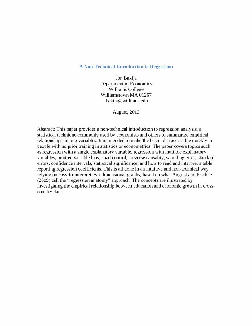
August, 2013 Abstract: This paper provides a non-technical introduction to regression analysis, a statistical technique commonly used by economists and others to summarize empirical relationships among variables. It is intended to make the basic idea accessible quickly to people with no prior training in statistics or econometrics. The paper covers topics such as regression with a single explanatory variable, regression with multiple explanatory variables, omitted variable bias, “bad control,” reverse causality, sampling error, standard errors, confidence intervals, statistical significance, and how to read and interpret a table reporting regression coefficients. This is all done in an intuitive and non-technical way relying on easy-to-interpret two-dimensional graphs, based on what Angrist and Pischke (2009) call the “regression anatomy” approach. The concepts are illustrated by investigating the empirical relationship between education and economic growth in cross-country data.

Introduction

A regression is a statistical technique for summarizing the empirical relationship between

a variable and one or more other variables. In economics, regression analysis is, by far,

the most commonly used statistical tool for discovering and communicating empirical

evidence. This paper provides a non-technical introduction to regression analysis,

illustrating the basic principles through an example using real-world data to address the

following question: how does education affect the rate of economic growth? The goals of

this paper are to help the reader understand the basic idea of what a regression means,

learn how to read and interpret a table that presents estimates from a regression, and

begin to appreciate some of the reasons why a regression may or may not provide

credible evidence on any particular question. Introductory textbooks and courses in

statistics and econometrics can provide you with a deeper, more mathematically

sophisticated, and more precise understanding of regression analysis.1 The purpose of

this paper is just to give you a sense of the forest, before you delve into examining the

individual trees.

The Question and the Data

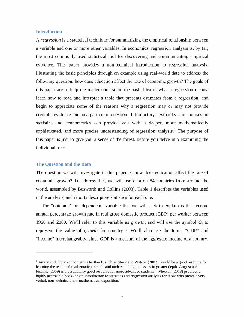
The question we will investigate in this paper is: how does education affect the rate of

economic growth? To address this, we will use data on 84 countries from around the

world, assembled by Bosworth and Collins (2003). Table 1 describes the variables used

in the analysis, and reports descriptive statistics for each one.

The “outcome” or “dependent” variable that we will seek to explain is the average

annual percentage growth rate in real gross domestic product (GDP) per worker between

1960 and 2000. We’ll refer to this variable as growth, and will use the symbol Gi to

represent the value of growth for country i. We’ll also use the terms “GDP” and

“income” interchangeably, since GDP is a measure of the aggregate income of a country.

1 Any introductory econometrics textbook, such as Stock and Watson (2007), would be a good resource for learning the technical mathematical details and understanding the issues in greater depth. Angrist and Pischke (2009) is a particularly good resource for more advanced students. Wheelan (2013) provides a highly accessible book-length introduction to statistics and regression analysis for those who prefer a very verbal, non-technical, non-mathematical exposition.

1

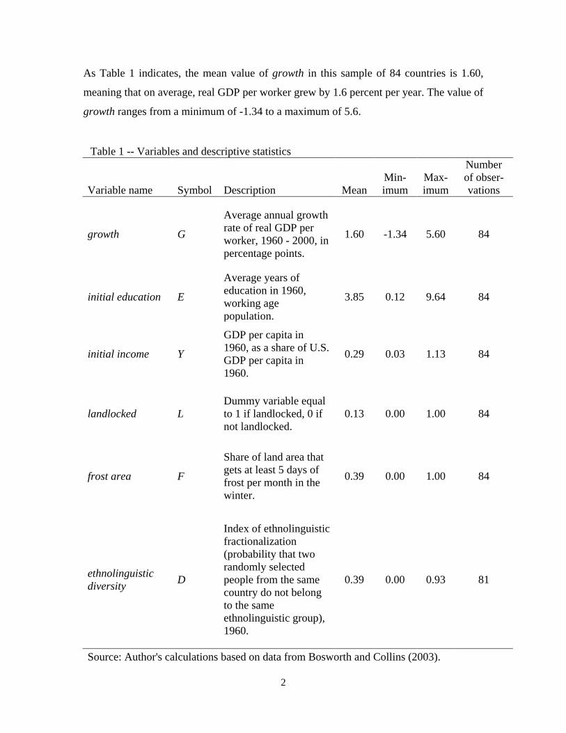
As Table 1 indicates, the mean value of growth in this sample of 84 countries is 1.60,

meaning that on average, real GDP per worker grew by 1.6 percent per year. The value of

growth ranges from a minimum of -1.34 to a maximum of 5.6.

Table 1 -- Variables and descriptive statistics

Variable name Symbol Description Mean Min-imum

Max-imum

Number of obser-vations

growth G

Average annual growth rate of real GDP per worker, 1960 - 2000, in percentage points.

1.60 -1.34 5.60 84

initial education E

Average years of education in 1960, working age population.

3.85 0.12 9.64 84

initial income Y

GDP per capita in 1960, as a share of U.S. GDP per capita in 1960.

0.29 0.03 1.13 84

landlocked L Dummy variable equal to 1 if landlocked, 0 if not landlocked.

0.13 0.00 1.00 84

frost area F

Share of land area that gets at least 5 days of frost per month in the winter.

0.39 0.00 1.00 84

ethnolinguistic diversity D

Index of ethnolinguistic fractionalization (probability that two randomly selected people from the same country do not belong to the same ethnolinguistic group), 1960.

0.39 0.00 0.93 81

Source: Author's calculations based on data from Bosworth and Collins (2003).

2

The main “independent” or “explanatory” variable of interest is the average number of

years of educational attainment among working-age people in the country in 1960. We’ll

refer to this as initial education, and will use Ei to symbolize the value of initial

education for country i. The goal of our regression analysis will be to learn something

about whether, and to what extent, countries with a higher initial level of educational

attainment experienced better subsequent economic growth, eventually holding constant

the effects of some other variables. There are numerous sensible reasons why, in theory,

education might have a positive effect on economic growth. For example, education may

teach useful skills, making workers more productive, thus increasing GDP. In addition, a

better-educated nation might be better able to invent new technologies, or to adapt and

implement existing productive technologies borrowed from other countries. Education

could also improve the quality of country’s governance if it helps the citizens of a

country become better-informed voters and improves their ability to think critically.

Better governance might in turn improve economic growth, for example because it

reduces corruption, which can act like a tax, harming incentives to be productive, or

which can divert revenues that otherwise would have been used to finance government

expenditures that make the economy more productive.

Table 1 also includes information on four “control variables,” which are additional

explanatory variables that we might want to account for in our regression analysis.2 The

control variables are other variables which might have independent causal effects on

growth, and which might be correlated with initial education. In that case, if we omitted3

these other variables from our regression analysis, our regression would give us a

misleading (or “biased”) estimate of the causal effect of initial education on growth.

When we “control” for these other variables in our regression analysis, we will be able to

2 Every explanatory variable in a regression analysis can be considered a “control variable,” but sometimes economists tend to call the particular explanatory variable that we are most interested in, and that we are focusing on at the time, the “explanatory variable of interest,” and to call the other explanatory variables the control variables. 3 “To omit” means to “leave out.” So an omitted variable is a variable that is not included in our regression analysis. It might be omitted, for example, because it is impossible to measure or because we simply do not have any good data on it, or it might be omitted because it did not occur to us to include it, among other reasons.

3

say something about how a change in initial education would affect growth holding these

other factors constant.

The first control variable is initial income, symbolized by Yi. It represents the ratio of

per capita GDP in 1960 in country i to per capita GDP in the U.S. in 1960. Other things

equal, we would probably expect a country’s initial level of income to have an

independent negative effect on its subsequent economic growth rate – that is, countries

that start out poorer, other things equal, might be expected to experience higher rates of

economic growth, leading to “convergence” in levels of income across countries over

time. This idea is most closely associated with the work of Robert Solow (1957). The

idea is that in order to achieve sustained high rates of economic growth, countries that

start out at a high level of income per person need to do difficult things, such as

developing new technologies. Such countries tend to also already have a lot of physical

capital (e.g., factories, productive machinery) per worker, and diminishing marginal

returns to physical capital make it difficult for such countries to achieve high economic

growth rates solely through additional saving and investment. It might, in principle, be

easier for countries starting out with a lower level of income per person to achieve rapid

and sustained economic growth, because the technology they need to grow already exists

in other countries and they just need to copy it. In addition, countries that start out with

lower incomes also start out with low levels of physical capital per worker, so the

marginal benefit in terms of productivity from adding additional physical capital through

saving and investment can be very large. On the other hand, countries starting with low

levels of income per person tend to have all sorts of other problems, such as poor

governance, which make it more difficult for them to grow. So it is not obvious, without

examining the data, whether initial income should have a positive or negative effect on

subsequent economic growth.

For most of this paper, we’ll just focus on the relationship among growth, initial

education, and initial income, but we’ll also eventually consider some additional control

variables, which I’ll describe immediately below, to help illustrate some points that come

up much later in the paper.

4

The next two control variables are both indicators of geographic characteristics of a

country that might influence economic growth.4 The variable landlocked, symbolized by

Li, equals 1 if the country is landlocked (meaning it does not have any direct access to an

ocean) and zero if it is not landlocked.5 Landlocked is an example of a “dummy variable”

(also known as an “indicator variable”), meaning that the variable can take on just two

values, zero and one. Being landlocked may have a negative effect on economic growth,

for example because it makes it more difficult to engage in international trade, which

hinders the country’s ability to specialize and achieve gains from trade. Being landlocked

makes it harder for the country to interact with the outside world more generally,

reducing the country’s ability to learn about and adapt new technologies or to benefit

from inflows of capital investment from savers in the rest of the world. The variable frost

area, symbolized by Fi, represents the share of the land area in the country that gets at

least 5 days of frost (below-freezing ground temperatures) per month in the winter. This

variable is originally from Masters and MacMillan (2001), who suggest it as a good

summary measure of climactic conditions that might influence growth. When you look

around the globe, you’ll notice that most of the very poor countries are located nearer to

the equator, and most of the rich countries are located in temperate or cold climates.

Some economists have argued that this is not entirely an accident. Very warm climates

tend to be hospitable to disease-carrying or crop-destroying pests (e.g., malaria-infected

mosquitoes), and it can be difficult for some such pests to survive in frosty conditions.

Poor health and destroyed crops hinder economic productivity, and could conceivably

make it more difficult to take advantage of productivity-enhancing technological

advances happening in the rest of the world. For this reason, it makes sense that frost

area might have a positive influence on economic growth.

The final control variable we will consider is ethnolinguistic diversity, symbolized by

Di. An “ethnolinguistic group” is a group of people who historically spoke the same

native language and are of the same ethnicity. This variable represents the probability, as

of 1960, that two randomly selected people from country i do not belong to the same

4 For an interesting discussion of the role that geography might play in influencing economic growth, see Gallup, Sachs, and Mellinger (1999). 5 The original source of the landlocked variable is Rodrik et al. (2002)

5

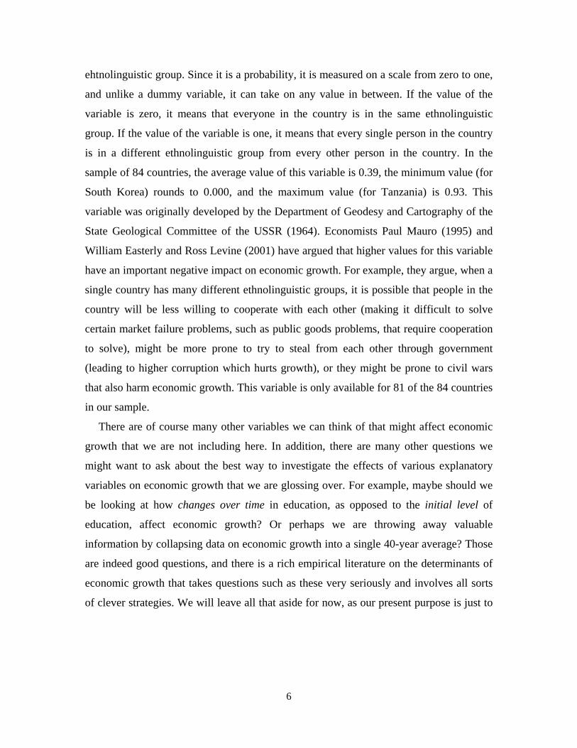
ehtnolinguistic group. Since it is a probability, it is measured on a scale from zero to one,

and unlike a dummy variable, it can take on any value in between. If the value of the

variable is zero, it means that everyone in the country is in the same ethnolinguistic

group. If the value of the variable is one, it means that every single person in the country

is in a different ethnolinguistic group from every other person in the country. In the

sample of 84 countries, the average value of this variable is 0.39, the minimum value (for

South Korea) rounds to 0.000, and the maximum value (for Tanzania) is 0.93. This

variable was originally developed by the Department of Geodesy and Cartography of the

State Geological Committee of the USSR (1964). Economists Paul Mauro (1995) and

William Easterly and Ross Levine (2001) have argued that higher values for this variable

have an important negative impact on economic growth. For example, they argue, when a

single country has many different ethnolinguistic groups, it is possible that people in the

country will be less willing to cooperate with each other (making it difficult to solve

certain market failure problems, such as public goods problems, that require cooperation

to solve), might be more prone to try to steal from each other through government

(leading to higher corruption which hurts growth), or they might be prone to civil wars

that also harm economic growth. This variable is only available for 81 of the 84 countries

in our sample.

There are of course many other variables we can think of that might affect economic

growth that we are not including here. In addition, there are many other questions we

might want to ask about the best way to investigate the effects of various explanatory

variables on economic growth that we are glossing over. For example, maybe should we

be looking at how changes over time in education, as opposed to the initial level of

education, affect economic growth? Or perhaps we are throwing away valuable

information by collapsing data on economic growth into a single 40-year average? Those

are indeed good questions, and there is a rich empirical literature on the determinants of

economic growth that takes questions such as these very seriously and involves all sorts

of clever strategies. We will leave all that aside for now, as our present purpose is just to

6

illustrate how a regression works and what it means, not to provide thoroughly

convincing evidence on what factors cause economic growth.6

Regression with a Single Explanatory Variable

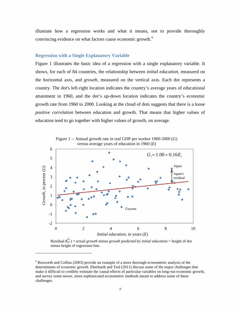
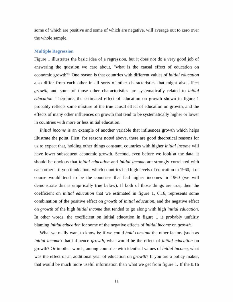
Figure 1 illustrates the basic idea of a regression with a single explanatory variable. It

shows, for each of 84 countries, the relationship between initial education, measured on

the horizontal axis, and growth, measured on the vertical axis. Each dot represents a

country. The dot's left-right location indicates the country’s average years of educational

attainment in 1960, and the dot’s up-down location indicates the country’s economic

growth rate from 1960 to 2000. Looking at the cloud of dots suggests that there is a loose

positive correlation between education and growth. That means that higher values of

education tend to go together with higher values of growth, on average.

6 Bosworth and Collins (2003) provide an example of a more thorough econometric analysis of the determinants of economic growth. Eberhardt and Teal (2011) discuss some of the major challenges that make it difficult to credibly estimate the causal effects of particular variables on long-run economic growth, and survey some newer, more sophisticated econometric methods meant to address some of these challenges.

-2

-1

0

1

2

3

4

5

6

0 2 4 6 8 10

Gro

wth

, in

perc

ent (

G)

Initial education, in years (E)

Figure 1 -- Annual growth rate in real GDP per worker 1960-2000 (G) versus average years of education in 1960 (E)

Residual ( ) = actual growth minus growth predicted by initial education = height of dot minus height of regression line.

Japan

Guyana

G

Japan's residual

ii EG 16.000.1 +=

7

The straight line drawn through the dots in figure 1 is the “ordinary least squares”

(OLS) regression line. A regression line is a straight line that summarizes the relationship

between two variables. The OLS regression line is meant to "fit" the cloud of dots as

closely as possible, in the sense of summarizing the average relationship between initial

education and growth. We will explain more precisely how it is computed and what it

means a bit later. The equation for the OLS regression line shown in figure 1 is:

Gi = 1.00 + 0.16Ei (1)

The height (or vertical axis value) of the regression line at a given level of initial

education (Ei) is 1.00 + 0.16(Ei). This represents the growth rate that the OLS regression

line "predicts" a country with that amount of education will have. The vertical axis

intercept of the regression line, 1.00, tells us the predicted value of growth for a country

with a value of zero for initial education. The slope of the regression line, 0.16, means

that each one year increase in initial education is associated, on average, with an increase

in the average annual growth rate in real GDP per worker of 0.16 percentage points. So

for example, if a country had a growth rate of 1 percent per year, and added a year of

education, its growth rate would be predicted to increase to 1.16 percent per year.

Similarly, the OLS regression line predicts that a country with 5 years of initial education

would have an average annual growth rate of 1.00 + 0.16×5 = 1.8 percent per year. The

estimated slope of the regression line, 0.16, is called the “coefficient” on initial

education. It is consistent with our intuition that initial education should have a positive

effect on growth, but it is not a very large positive effect.

For each country in figure 1, there is a difference between the actual value of growth

for that country, and the value of growth that is predicted for that country by the

regression line. The actual value of the dependent variable (in this case, growth) minus

the predicted value is called the “residual” or “error.” In other words, the residual for

each country is the height of that country’s “dot” minus the height of the regression line

at that country’s level for the explanatory variable (initial education). Countries with dots

above the line have positive residuals, and countries with dots below the line have

8

negative residuals. To help illustrate this, in figure 1, the dots for two particular countries,

Japan and Guyana, are labeled with the country names. Japan’s value of initial education

is 8.43, and based on that, the regression line predicts a value for growth of 1.00 +

0.16×8.43 = 2.35. Japan’s actual value of growth was 3.88. Japan’s residual is its actual

growth minus its predicted growth, 3.88 – 2.35 = 1.53. Guyana, on the other hand, has a

value of initial education of 4.78, and the regression line predicts a value of growth for

Guyana of 1.76. But Guyana’s actual value for growth was -0.25, so its residual equals

-0.25 -1.76 = -2.01 (that is, the residual for Guyana is negative 2.01). The residual can be

thought of as the portion of the dependent variable (in this case, growth) that is not

predicted by the explanatory variable (in this case, initial education). Many different

factors, including random chance, affect growth, and the residual reflects the influence of

these other factors.

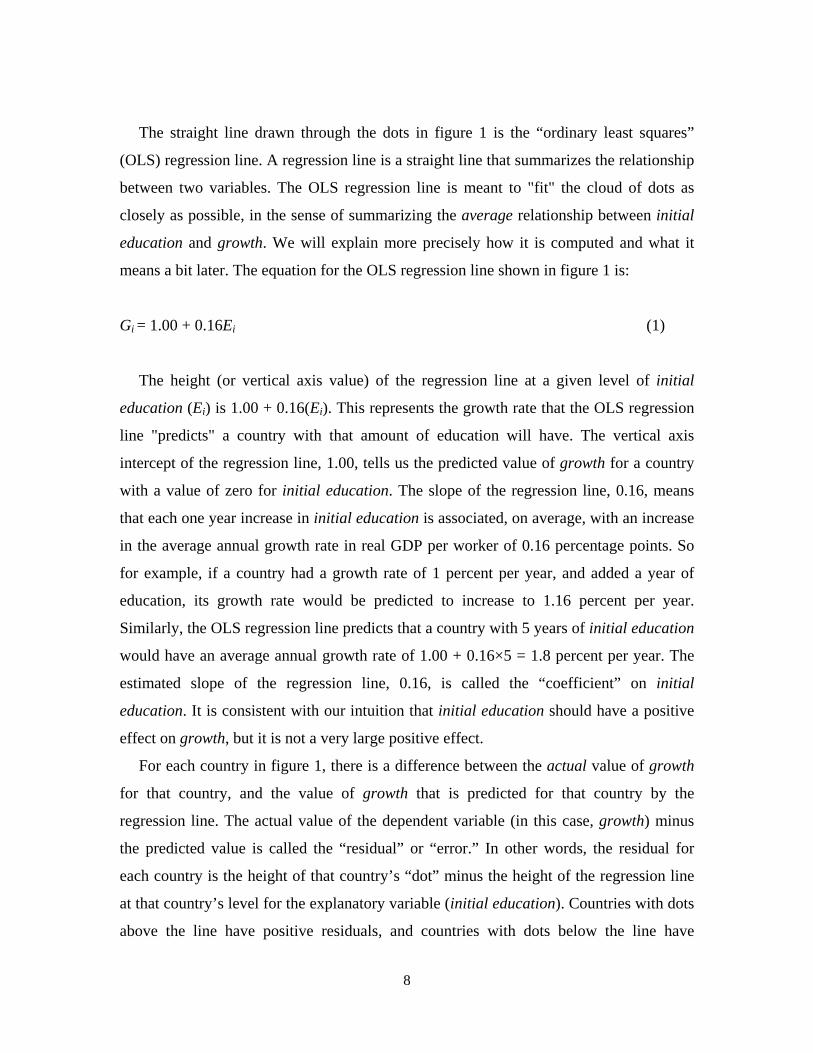
The value of the dependent variable for each observation (country) always equals the

value for that variable predicted by the regression, plus the residual. We will express this

relationship in abstract terms as:

𝐺𝑖 = 𝑏0 + 𝑏1𝐸𝑖 + �̈�𝑖 (2)

where Gi is the value of growth for country i (the dependent variable) b0 is the vertical

axis intercept of the regression line (equal to 1.00 in figure 1), b1 is the slope of the

regression line (that is, the coefficient on Ei, which is equal to 0.16 in figure 1), Ei is the

value of the explanatory variable initial education for country i, and �̈�𝑖 is the estimated

residual for observation i. For each distinct regression equation that we discuss in this

paper, we will use different symbols to represent the intercept, coefficients, and residuals,

because they will represent different numbers in different regressions.

There are actually many different possible methods for estimating a regression line. As

noted above, in figure 1 we used the “ordinary least squares” (OLS) method to estimate

Dependent variable

Intercept

Coefficient

Explanatory variable

Residual

9

the regression line, which is the most commonly used approach. OLS picks the unique

values for the intercept and slope for the regression line that minimize the sum of squared

residuals. This boils down to a calculus problem. First, recall that the residual (�̈�𝑖 in this

case) equals the actual value of the dependent variable minus the value of the dependent

variable predicted by the regression. So,

�̈�𝑖 = Gi – [b0 + b1Ei] (3)

Minimizing the sum of squared residuals, as OLS does, involves solving the following

calculus problem:

Choose b0 and b1 to minimize ∑ [𝐺𝑖 − (𝑏0 + 𝑏1𝐸𝑖)𝑖 ]2 (4)

We will not get into the details of how the math works here, but it is a straightforward

application of calculus.7 Many different software packages, including Excel and Stata,

can calculate OLS estimates of intercept and slope parameters for you.

Before moving on, we’ll note a couple of properties of the OLS estimator that will be

useful to know later. First, the OLS predicted value of the dependent variable is an

estimate of the conditional mean of the dependent variable, given the value of the

explanatory variable for that country. To put it another way, in figure 1, the value of

growth predicted by the OLS regression line at each level of education represents what is

in some sense the best estimate of the mean level of growth among countries with that

level of initial education that we can get when assuming that the relationship between

initial education and growth is described by a straight line. A second implication of the

math of OLS worth noting here is that the mean value of the estimated residuals will, by

construction, always be zero under this approach. That of course does not mean that each

individual estimated residual will be zero – rather, it simply means that the residuals,

7 See, for example, Stock and Watson (2007, Appendix to Chapter 4) for the derivation of the formulas for the OLS intercept and slope parameters using calculus. An example of another method for estimating a regression line, besides OLS, would be a “median regression,” which minimizes the sum of the absolute values of the residuals.

10

some of which are positive and some of which are negative, will average out to zero over

the whole sample.

Multiple Regression

Figure 1 illustrates the basic idea of a regression, but it does not do a very good job of

answering the question we care about, “what is the causal effect of education on

economic growth?” One reason is that countries with different values of initial education

also differ from each other in all sorts of other characteristics that might also affect

growth, and some of those other characteristics are systematically related to initial

education. Therefore, the estimated effect of education on growth shown in figure 1

probably reflects some mixture of the true causal effect of education on growth, and the

effects of many other influences on growth that tend to be systematically higher or lower

in countries with more or less initial education.

Initial income is an example of another variable that influences growth which helps

illustrate the point. First, for reasons noted above, there are good theoretical reasons for

us to expect that, holding other things constant, countries with higher initial income will

have lower subsequent economic growth. Second, even before we look at the data, it

should be obvious that initial education and initial income are strongly correlated with

each other – if you think about which countries had high levels of education in 1960, it of

course would tend to be the countries that had higher incomes in 1960 (we will

demonstrate this is empirically true below). If both of those things are true, then the

coefficient on initial education that we estimated in figure 1, 0.16, represents some

combination of the positive effect on growth of initial education, and the negative effect

on growth of the high initial income that tended to go along with high initial education.

In other words, the coefficient on initial education in figure 1 is probably unfairly

blaming initial education for some of the negative effects of initial income on growth.

What we really want to know is: if we could hold constant the other factors (such as

initial income) that influence growth, what would be the effect of initial education on

growth? Or in other words, among countries with identical values of initial income, what

was the effect of an additional year of education on growth? If you are a policy maker,

that would be much more useful information than what we get from figure 1. If the 0.16

11

estimate that we came up with in figure 1 reflects the combined positive effect of initial

education and negative effect of initial income, then it does not tell us anything about

what would happen to growth in any particular country if the government of the country

managed to increase average educational attainment by one year, without changing initial

income (obviously, governments have no direct control over initial income). Our 0.16

estimate from figure 1 is a biased estimate of the thing that we are really interested in

measuring, the causal effect of education on growth (holding other factors that influence

growth constant) -- meaning that it will be systematically wrong on average. Our story

above suggests that 0.16 is probably a downwardly biased estimate of what we want to

know – in other words, the story we told about initial income gives us good reason to

believe that 0.16 is systematically lower than the true causal effect of effect of education

on growth holding other things constant.

This is where a multiple regression can help us. A multiple regression is a technique

that is analogous to a regression with a single explanatory variable, like the one we

described above, except now there are multiple explanatory variables. So for example, we

can write out a linear equation that relates the dependent variable (growth, or Gi) to two

explanatory variables (initial education, or Ei, and initial income, or Yi). Equation (5)

below does exactly that:

Gi = β0 + β1Ei + β2Yi (5)

where β0 is the intercept, β1 is the slope coefficient on initial education (Ei), and β2 is the

slope coefficient on initial income (Yi).

The right-hand side of the equation above now represents the predicted value of a

country’s growth given its values of initial education and initial income. In each case, the

actual value of the dependent variable (growthi, also known as Gi) may differ from the

value predicted by the regression equation, and the difference (actual Gi minus predicted

Gi) is the residual. We’ll label the residual in this equation εi. The regression equation can

be estimated by ordinary least squares, which now selects β0, β1, and β2 to minimize the

sum of squared residuals εi. Doing so yields the following estimated relationship:

12

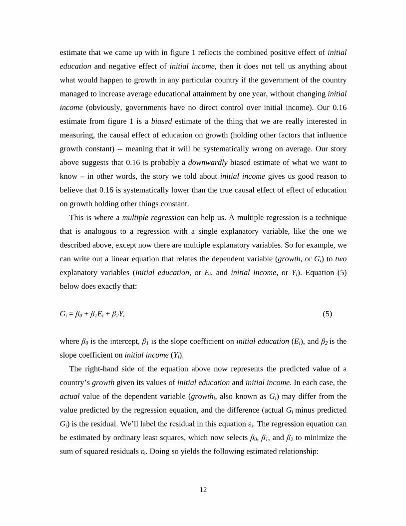
Gi = 0.94 + 0.49Ei -4.15Yi (6)

In the multiple regression equation, β1, which is estimated to be 0.49, now represents

the change in growth (Gi) associated with a one unit increase in initial education (Ei)

holding initial income (Yi) constant. So, we would say that controlling for initial income,

a one year increase in initial education is associated with a 0.49 percentage point increase

in the annual economic growth rate. This is a much larger effect than the 0.16 percentage

point increase suggested by figure 1. β2, the coefficient on initial income (Yi), is -4.15,

which means that controlling for initial education, increasing initial income by one unit

(where one unit is equal to the U.S. level of per capita GDP in 1960, a very large change)

is associated with an annual growth rate that is 4.15 percentage points lower. When a one

unit change in the explanatory variable is a very large change, it is sometimes useful to

report the predicted effect of a smaller change that is more within the range of typical

differences we see in the data. For example, dividing the β2 coefficient by 10 gives us the

effect of increasing initial income by 1/10th of the U.S. level of initial income, holding

initial education constant. So a country that starts out with initial income equal to 50

percent of that of the U.S., instead of 40 percent, holding initial education constant, is

predicted to experience an annual growth rate that is 0.415 percentage points lower as a

result. Thus, once we control for initial education, the sign of the effect of initial income

on growth is negative, consistent with what the “convergence” theories we discussed

earlier would predict.

To better understand what the β1 coefficient in a multiple regression means, consider

the following example. Imagine there were a large number of pairs of countries, where

each pair of countries had identical levels of initial income, but differed in initial

education by exactly one year. If we estimated multiple regression equation (5) above on

such data, the coefficient β1 on initial education would be precisely the growth rate of the

country with one more year of education minus the growth rate of the country with one

less year of education within each pair of countries with identical income, averaged over

all pairs. So for example, if there were three such pairs of countries, and the growth rate

of the country with one extra year of education in each pair was 0.2 percentage points

higher in the first pair, 0.7 percentage points higher in the second pair, and 0.3 percentage

13

points higher in the third pair, our estimate of β1 would be the average of those

differences, (0.2 + 0.7 + 0.3) / 3 = 0.4. So in other words, β1 would be the answer to the

question: “among countries with exactly the same level of initial income, what is the

average difference in growth rates associated with one more year of initial education.”

That’s what we want to know.

In practice, available data rarely include a complete set of perfectly matched pairs,

each with identical values of the control variable and with values of the key explanatory

variable of interest that differ by exactly one unit. In the more general case where the

relevant variables vary more continuously than that, the OLS multiple regression

coefficient β1 still gets at exactly the same concept as described in the previous

paragraph, but how it gets there is a bit more complicated to understand, and it relies

more heavily on the assumption of straight-line relationships among the variables. In this

setting, the OLS estimate of β1 uses the data we actually have to compute our best

estimate of what the average difference in growth rates between countries with identical

initial income levels but initial education values differing by one year would be, under

the assumption that the relationships among variables growth, initial income, and initial

education are well-described by equations for straight lines. In the next section, we’ll

work through some graphs which provide a clearer sense of what this means.

An equation for a multiple regression with two explanatory variables, such as (5), is an

equation for a two-dimensional plane in 3-dimensional space. Imagine a graph with 3

axes. There are two horizontal axes that are perpendicular to each other – one measuring

the value of initial education and the other measuring the value for initial income – and

one vertical axis measuring growth. Imagine starting with figure 1 above, and adding a

third axis for initial income that starts at the origin of figure 1, and pops out of the page at

you, exactly perpendicular to the two-dimensional plane formed by the page. The cloud

of dots would then be floating in 3-dimensional space, with 3-dimensional coordinates

reflecting the values of the three variables for each country. Countries with higher values

of initial income would have dots that pop out of the page more (i.e., closer to your eyes).

The OLS multiple regression is a 2-dimensional plane that summarizes that cloud of

points, minimizing the sum of squared residuals.

14

The “Regression Anatomy” Way of Understanding Multiple Regression

If you are like most humans, attempting to visualize a multiple regression in 3-

dimensional space is not very helpful to understanding what the thing actually means, and

attempting to visualize a multiple regression with more than two explanatory variables

(thus necessitating more than 3 dimensions) is impossible. For this reason, it is helpful to

break down what is going on in the multiple regression equation described above into

component 2-dimensional parts. Angrist and Pischke (2009) call this the “regression

anatomy” approach. Just as physical anatomy shows how the component parts of the

body fit together to make the whole work, the regression anatomy approach

mathematically decomposes a multiple regression into a set of regressions that each have

just one explanatory variable, and it shows how they fit together to make the whole

multiple regression work.

Figures 2, 3, and 4 below illustrate the regression anatomy approach to estimating β1.

The purpose of our multiple regression is to estimate the effect of initial education on

growth, removing the effects of initial income from each one. The regression anatomy

approach does exactly that. Figures 2 and 3 show how we can decompose growth and

initial education into the parts that are and are not predicted by initial income, and then

figure 4 shows the relationship between the portions of growth and initial education that

are not predicted by initial income. The slope of the relationship in figure 4 will be

exactly the β1 coefficient that we are looking for.

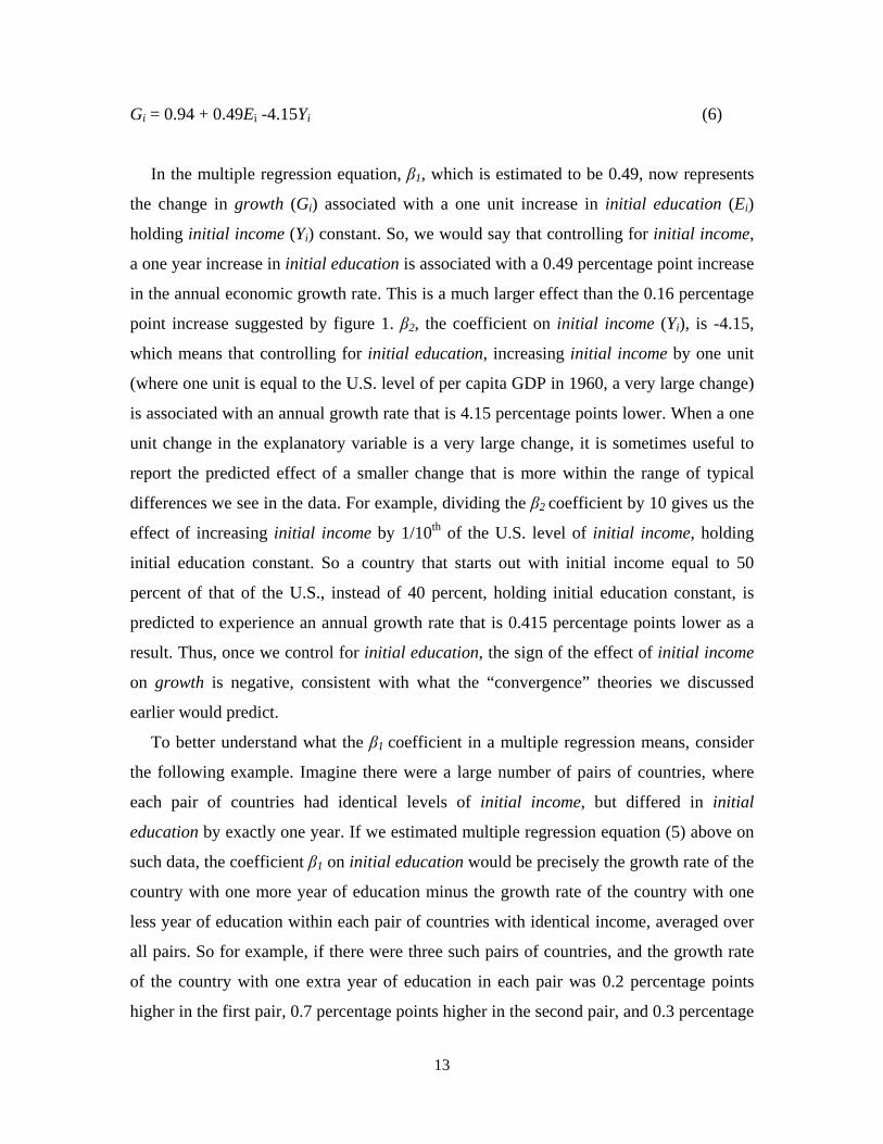
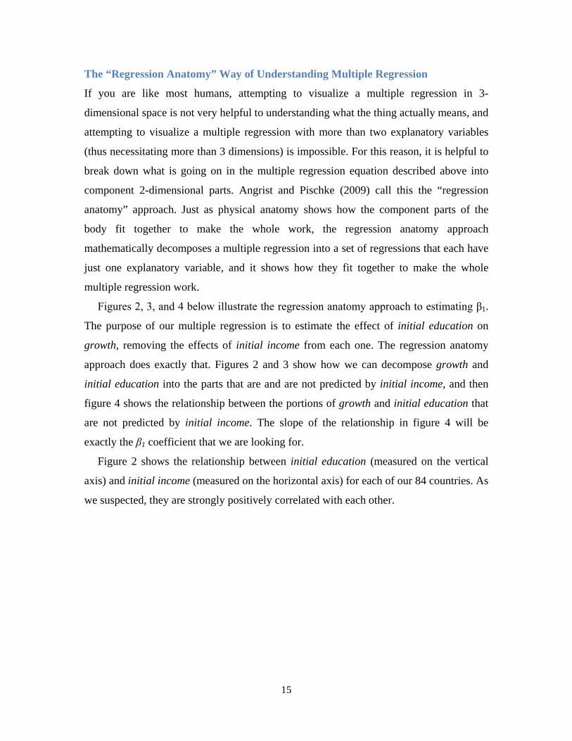
Figure 2 shows the relationship between initial education (measured on the vertical

axis) and initial income (measured on the horizontal axis) for each of our 84 countries. As

we suspected, they are strongly positively correlated with each other.

15

The OLS regression line through the cloud of points in figure 2, in abstract terms, is:

𝐸𝑖 = 𝑎0 + 𝑎1𝑌𝑖 (7)

The estimated value of 𝑎1 is 9.17, meaning a one unit increase in initial income (i.e.,

from zero to the level of U.S. per capita GDP in 1960) is associated with 9.17 more years

of initial education.

In figure 2, the main thing we care about for the purpose of ultimately estimating β1 is

the residual, which we will call E�𝑖. Recall that the residual represents the actual value of

the dependent variable (in this case, initial education), minus value of that variable that

would be predicted based on the explanatory variable (in this case, initial income). Or in

symbols, E�i = 𝐸𝑖 − (𝑎0 + 𝑎1𝑌𝑖). Also recall that our goal is to get β1, which represents

the effect of initial education on growth removing the effects of initial income from each

one. The residuals in figure 2 give us one part of what we need to do that: E�𝑖 is a measure

of the portion initial education that is different from what you would predict based on

0 1 2 3 4 5 6 7 8 9

10

0.0 0.2 0.4 0.6 0.8 1.0 1.2

Initi

al e

duca

tion,

in y

ears

(E)

Initial income, ratio to U.S. level (Y)

Figure 2 -- Average years of education in 1960 (E) versus per capita GDP relative to U.S. in 1960 (Y)

Residual ( ) = actual initial education minus initial education predicted based on initial income = height of dot minus height of regression line.

E~

ii YE 17.918.1 +=

16

initial income, or in other words, it is a measure of initial education removing the effects

of initial income. Or to put it another way, our goal is to get a measure of how initial

education differs among countries with similar levels of initial income, and 𝐸�𝑖 is one

good way of measuring that.

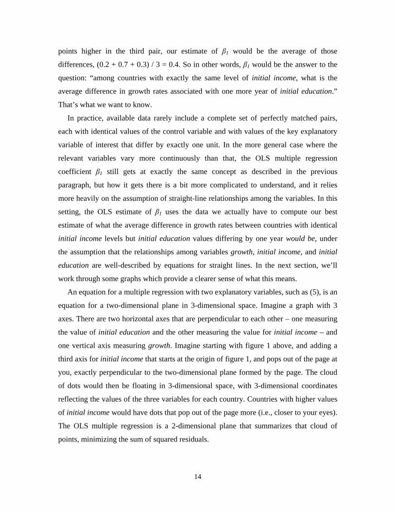
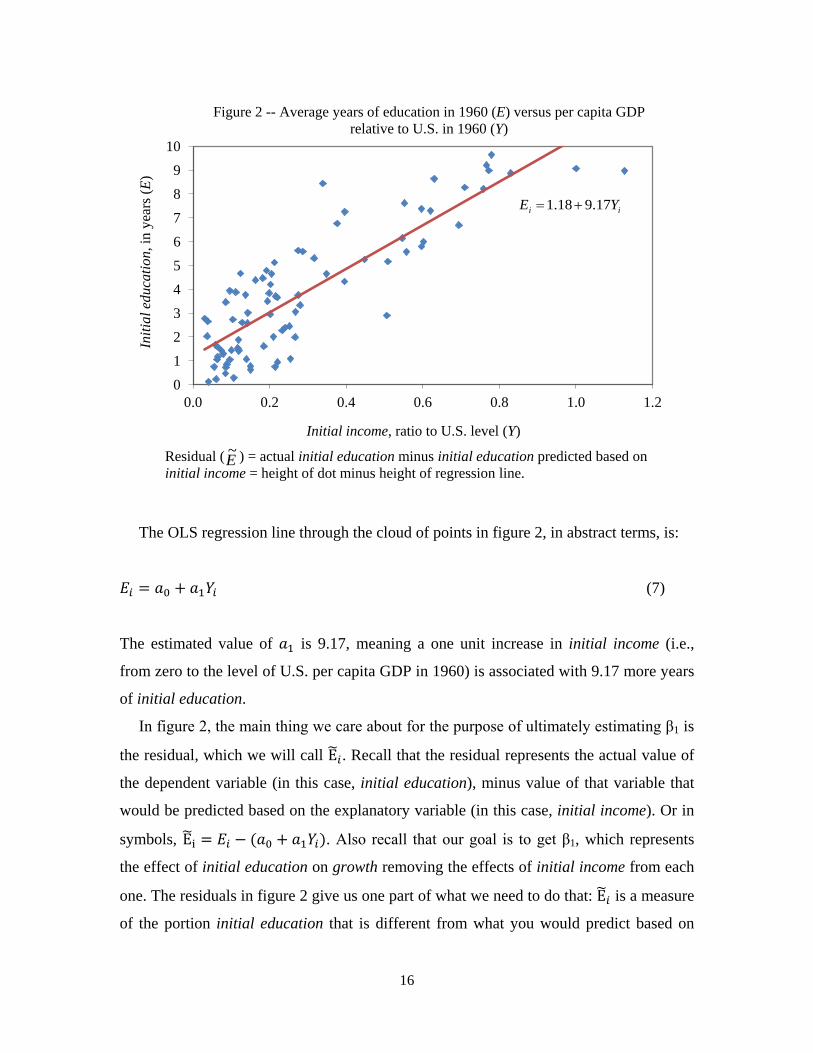
Figure 3 shows the relationship between growth (measured on the vertical axis) and

initial income (measured on the horizontal axis) for each of our 84 countries. In figure 3,

the correlation between growth and initial income is positive but not very strong.

The OLS regression line through the cloud of points shown in figure 3, in abstract

terms, is:

𝐺𝑖 = 𝑐0 + 𝑐1𝑌𝑖 (8)

The estimated value of 𝑐1 is 0.31, which suggests that a one unit increase in initial

income is associated with a 0.31 percentage point increase in growth. We should not take

this as a refutation of our earlier theory that high initial income hurts growth, however.

That theory said that higher initial income should be associated with lower subsequent

economic growth holding other things constant. Figure 3 does not hold anything else

constant. In particular, it does not hold initial education constant. So (as we will prove

later below), the 0.31 slope coefficient estimate reflects a combination of the negative

effect on growth of initial income, and the positive effect on growth of the high initial

education that goes along with high initial income. Remember, back in equation (6), we

estimated that the effect of initial income on growth holding initial education constant

was indeed negative.

17

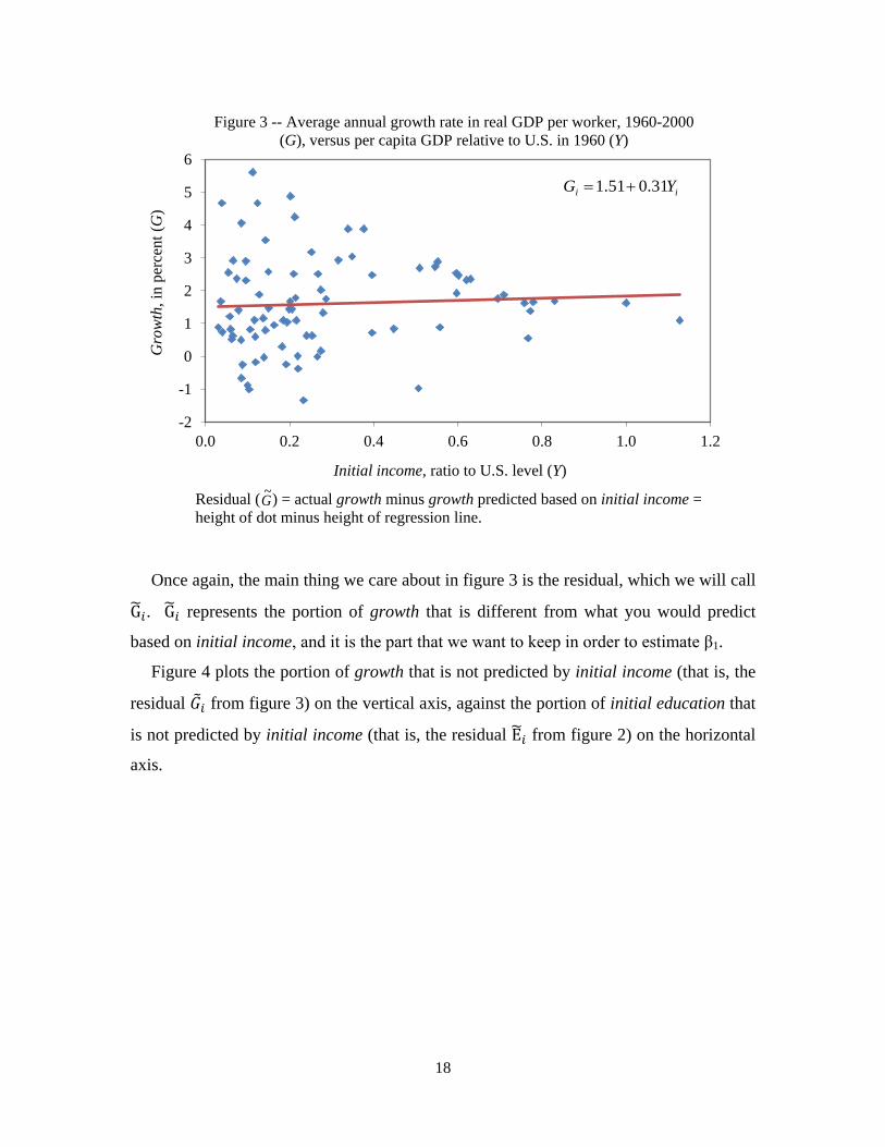
Once again, the main thing we care about in figure 3 is the residual, which we will call

G�𝑖. G�𝑖 represents the portion of growth that is different from what you would predict

based on initial income, and it is the part that we want to keep in order to estimate β1.

Figure 4 plots the portion of growth that is not predicted by initial income (that is, the

residual 𝐺�𝑖 from figure 3) on the vertical axis, against the portion of initial education that

is not predicted by initial income (that is, the residual E�𝑖 from figure 2) on the horizontal

axis.

-2

-1

0

1

2

3

4

5

6

0.0 0.2 0.4 0.6 0.8 1.0 1.2

Gro

wth

, in

perc

ent (

G)

Initial income, ratio to U.S. level (Y)

Figure 3 -- Average annual growth rate in real GDP per worker, 1960-2000 (G), versus per capita GDP relative to U.S. in 1960 (Y)

Residual ( ) = actual growth minus growth predicted based on initial income = height of dot minus height of regression line.

G~

ii YG 31.051.1 +=

18

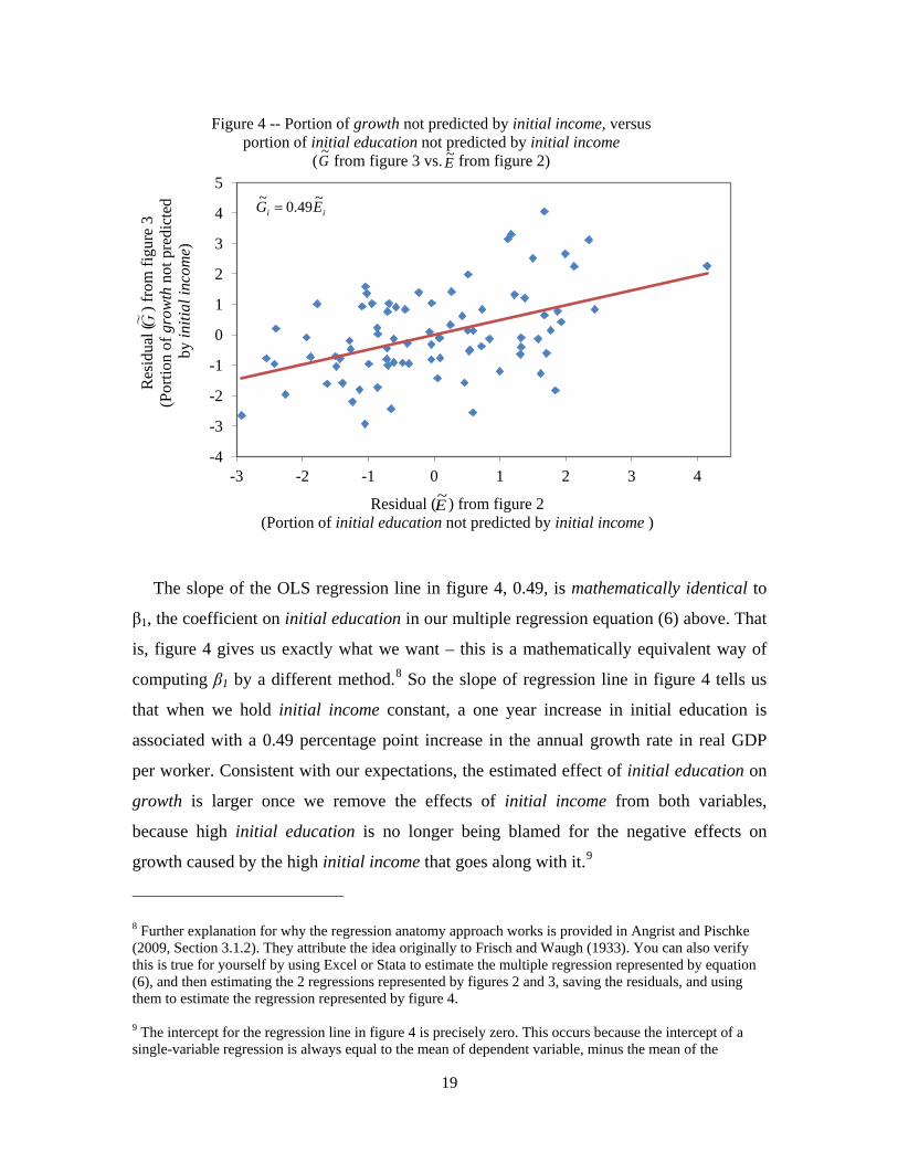
The slope of the OLS regression line in figure 4, 0.49, is mathematically identical to

β1, the coefficient on initial education in our multiple regression equation (6) above. That

is, figure 4 gives us exactly what we want – this is a mathematically equivalent way of

computing β1 by a different method.8 So the slope of regression line in figure 4 tells us

that when we hold initial income constant, a one year increase in initial education is

associated with a 0.49 percentage point increase in the annual growth rate in real GDP

per worker. Consistent with our expectations, the estimated effect of initial education on

growth is larger once we remove the effects of initial income from both variables,

because high initial education is no longer being blamed for the negative effects on

growth caused by the high initial income that goes along with it.9

8 Further explanation for why the regression anatomy approach works is provided in Angrist and Pischke (2009, Section 3.1.2). They attribute the idea originally to Frisch and Waugh (1933). You can also verify this is true for yourself by using Excel or Stata to estimate the multiple regression represented by equation (6), and then estimating the 2 regressions represented by figures 2 and 3, saving the residuals, and using them to estimate the regression represented by figure 4. 9 The intercept for the regression line in figure 4 is precisely zero. This occurs because the intercept of a single-variable regression is always equal to the mean of dependent variable, minus the mean of the

-4

-3

-2

-1

0

1

2

3

4

5

-3 -2 -1 0 1 2 3 4

Res

idua

l (

) fro

m fi

gure

3

(Por

tion

of g

row

th n

ot p

redi

cted

b

y in

itial

inco

me)

Residual ( ) from figure 2 (Portion of initial education not predicted by initial income )

Figure 4 -- Portion of growth not predicted by initial income, versus portion of initial education not predicted by initial income

( from figure 3 vs. from figure 2) G~ E~

E~

ii EG ~49.0~=

19

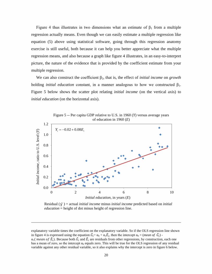
Figure 4 thus illustrates in two dimensions what an estimate of β1 from a multiple

regression actually means. Even though we can easily estimate a multiple regression like

equation (5) above using statistical software, going through this regression anatomy

exercise is still useful, both because it can help you better appreciate what the multiple

regression means, and also because a graph like figure 4 illustrates, in an easy-to-interpret

picture, the nature of the evidence that is provided by the coefficient estimate from your

multiple regression.

We can also construct the coefficient β2, that is, the effect of initial income on growth

holding initial education constant, in a manner analogous to how we constructed β1.

Figure 5 below shows the scatter plot relating initial income (on the vertical axis) to

initial education (on the horizontal axis).

explanatory variable times the coefficient on the explanatory variable. So if the OLS regression line shown in figure 4 is expressed using the equation 𝐺�𝑖= α0 + α1𝐸�𝑖, then the intercept α0 = (mean of 𝐺�𝑖) - α1( 𝑚𝑒𝑎𝑛 𝑜𝑓 𝐸�𝑖). Because both 𝐺�𝑖 and 𝐸�𝑖 are residuals from other regressions, by construction, each one has a mean of zero, so the intercept α0 equals zero. This will be true for the OLS regression of any residual variable against any other residual variable, so it also explains why the intercept is zero in figure 6 below.

0.0

0.2

0.4

0.6

0.8

1.0

1.2

0 2 4 6 8 10

Initi

al in

com

e, ra

tio to

U.S

. lev

el (Y

)

Initial education, in years (E)

Figure 5 -- Per capita GDP relative to U.S. in 1960 (Y) versus average years of education in 1960 (E)

Residual ( ) = actual initial income minus initial income predicted based on initial education = height of dot minus height of regression line.

Y

ii EY 08.002.0 +−=

20

We’ll express the equation for the OLS regression line in figure 5 as:

𝑌𝑖 = 𝑑0 + 𝑑1𝐸𝑖 (9)

The residual in figure 5, which we’ll call �̈�, represents the portion of initial income not

predicted by initial education, and it is the part that we want to keep in order to estimate

β2. The other thing we need to estimate β2 is the portion of growth not predicted by initial

education, which is the residual (�̈�) from figure 1 (which plotted the relationship between

growth on the vertical axis and initial education on the horizontal axis).

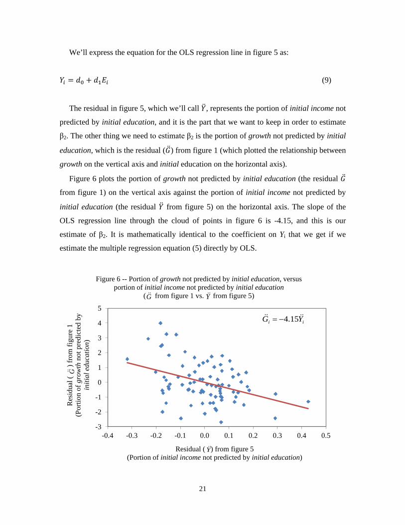
Figure 6 plots the portion of growth not predicted by initial education (the residual �̈�

from figure 1) on the vertical axis against the portion of initial income not predicted by

initial education (the residual �̈� from figure 5) on the horizontal axis. The slope of the

OLS regression line through the cloud of points in figure 6 is -4.15, and this is our

estimate of β2. It is mathematically identical to the coefficient on Yi that we get if we

estimate the multiple regression equation (5) directly by OLS.

-3

-2

-1

0

1

2

3

4

5

-0.4 -0.3 -0.2 -0.1 0.0 0.1 0.2 0.3 0.4 0.5

Res

idua

l (

) fr

om fi

gure

1

(Por

tion

of g

row

th n

ot p

redi

cted

by

initi

al e

duca

tion)

Residual ( ) from figure 5 (Portion of initial income not predicted by initial education)

Figure 6 -- Portion of growth not predicted by initial education, versus portion of initial income not predicted by initial education

( from figure 1 vs. from figure 5)

G

G Y

ii YG 15.4−=

Y

21

Now we have a basic understanding of what a multiple regression means. But to be an

informed consumer of regression analysis, it is also important to have a solid

understanding of why a regression analysis might provide misleading answer to the

question it is meant to investigate. There are many different ways that a regression

analysis can go wrong. In what follows, I’ll provide brief introductions to four of the

most important categories of potential problems: omitted variable bias, bad control,

reverse causality, and sampling error. After that, I’ll discuss ways to quantify the degree

of uncertainty arising from sampling error, introducing concepts such as “standard error,”

“confidence interval,” and “statistical significance,” and will point out some common

confusions about these concepts that you should be careful to avoid right from the outset.

Finally, I’ll go through an example of a table presenting coefficient estimates from

regressions based on the data described above, and explain how to interpret such a table.

Omitted Variable Bias When the purpose of our regression is to estimate the causal effect of one variable on

another variable, holding other things constant, as it usually is, one of the most serious

challenges we face is the problem of omitted variable bias. Omitted variable bias means

that our estimate of the effect of one variable on another variable is a biased

(systematically wrong on average) estimate of the causal effect we want to estimate,

because we’ve omitted (left out) another variable from the regression. It occurs whenever

we omit a variable which affects the dependent (outcome) variable and is correlated with

one or more of the explanatory variables that are included on the right-hand-side of our

regression. The example we worked through above can help us to understand omitted

variable bias, and to understand the likely direction of bias in a variety of scenarios.

Consider again figure 1. In that figure, the estimated effect of an additional year of

initial education on growth, 0.16, is a biased estimate of what we want to know, the

causal effect of initial education on growth holding other things constant. As we

demonstrated above, initial income also affects growth and is correlated with initial

education, so it is a source of omitted variable bias in the short regression of growth on

initial education -- equation (1), illustrated in figure 1. Including initial income as a

22

control variable, as we did in the long (multiple) regression shown in equation (5), solves

that particular source of omitted variable bias.

It turns out that there is a precise mathematical relationship among the coefficients in

the “short” regressions (the various regressions with just one explanatory variable) and

the coefficients in the long regression (the multiple regression in equation 5, with two

explanatory variables) that we estimated in our example above. We can express the

relationship between a short regression coefficient and the corresponding long regression

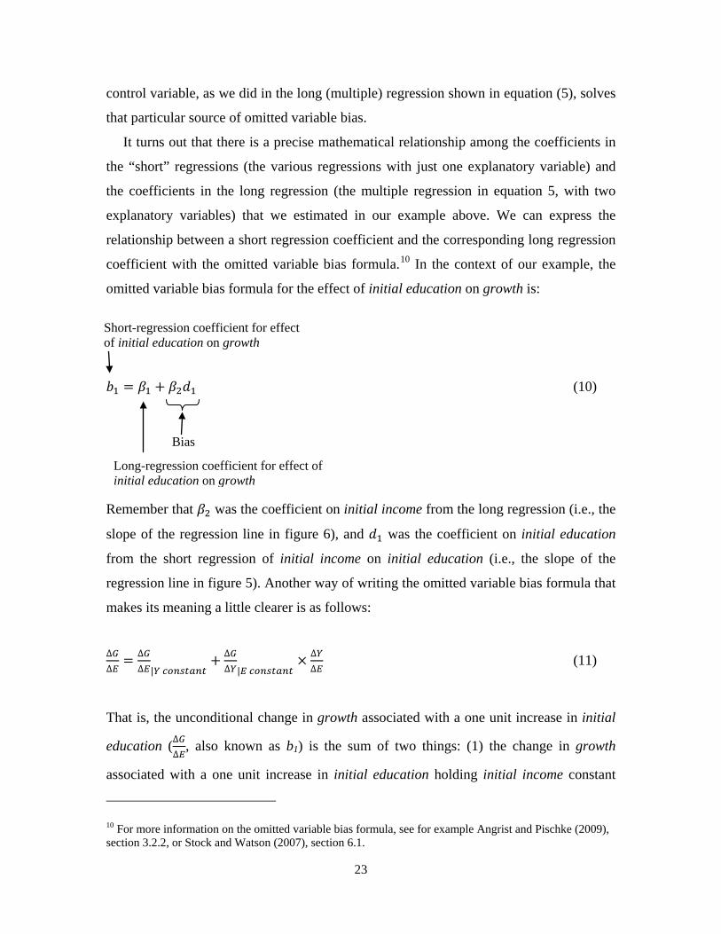
coefficient with the omitted variable bias formula.10 In the context of our example, the

omitted variable bias formula for the effect of initial education on growth is:

𝑏1 = 𝛽1 + 𝛽2𝑑1 (10)

Remember that 𝛽2 was the coefficient on initial income from the long regression (i.e., the

slope of the regression line in figure 6), and 𝑑1 was the coefficient on initial education

from the short regression of initial income on initial education (i.e., the slope of the

regression line in figure 5). Another way of writing the omitted variable bias formula that

makes its meaning a little clearer is as follows:

∆𝐺∆𝐸

= ∆𝐺∆𝐸|𝑌 𝑐𝑜𝑛𝑠𝑡𝑎𝑛𝑡

+ ∆𝐺∆𝑌|𝐸 𝑐𝑜𝑛𝑠𝑡𝑎𝑛𝑡

× ∆𝑌∆𝐸

(11)

That is, the unconditional change in growth associated with a one unit increase in initial

education (∆𝐺∆𝐸

, also known as b1) is the sum of two things: (1) the change in growth

associated with a one unit increase in initial education holding initial income constant

10 For more information on the omitted variable bias formula, see for example Angrist and Pischke (2009), section 3.2.2, or Stock and Watson (2007), section 6.1.

Short-regression coefficient for effect of initial education on growth

Long-regression coefficient for effect of initial education on growth

Bias

23

(∆𝐺∆𝐸|𝑌 𝑐𝑜𝑛𝑠𝑡𝑎𝑛𝑡

, also known as β1); and the change in growth associated with a one unit

increase in initial income holding initial education constant (∆𝐺∆𝑌|𝐸 𝑐𝑜𝑛𝑠𝑡𝑎𝑛𝑡

, also known as

β2), times the unconditional change in initial income associated with a one unit increase

in initial education (∆𝑌∆𝐸

, also known as d1).

We can verify that the omitted variable bias formula is correct by substituting in the

estimated values of each coefficient into equation (10):

0.16 = 0.49 + (-4.15)×(0.08) (12)

Do the math in equation (12) and you’ll see that the omitted variable bias formula is

indeed correct (aside from a bit of rounding error arising from the fact we’ve rounded the

coefficients to two decimal places).

If our goal were to estimate 𝛽1, then 𝑏1 is a misleading indicator of that. The omitted

variable bias formula clarifies what we would need to know to determine the size and

direction of the bias. The formula says that the 𝑏1 coefficient combines the effect of

initial education on growth holding initial income constant (𝛽1) with a bias term 𝛽2𝑑1.

Even if we had only estimated the short regression of growth on initial education

(equation 1), we could come up with a pretty good guess at the direction of bias (up or

down) if we thought carefully about the problem. This is an important part of critical

thinking about regression estimates, especially given that we can often think of relevant

variables that are not included in the analysis and that may not even be measurable. The

direction of bias can matter a lot for the practical implications of the regression evidence.

For instance, if we have a plausible omitted variable story that probably suggests the

estimated coefficient on initial education is too small, that would tend to strengthen the

case for investing in education, whereas if the omitted variable bias story suggests that

the estimated coefficient is too big, that would weaken the case. The omitted variable bias

formula helps us think clearly about these sorts of things.

In general, the sign of the bias depends on the sign of the long-regression coefficient

on the omitted variable, times sign of the correlation between the included explanatory

variable and the omitted variable. Recall that our intuitive story for the bias caused by

24

omitting initial income was as follows. In the short regression of growth on initial

education shown in figure 1, higher levels of initial education were being unfairly

blamed for the negative effects on growth of the higher levels of initial income

(implicitly, a statement that 𝛽2 is negative) that tend to go along with higher initial

education (implicitly a statement that 𝑑1 is positive). So, we guessed that the true effect

of initial education on growth holding initial income constant (𝛽1) would be larger than

𝑏1 (or in other words, we surmised that 𝑏1 was downwardly biased as an estimate of 𝛽1).

The omitted variable bias formula confirms our intuition that when 𝛽2 is negative and 𝑑1

is positive, 𝛽1 will be greater than 𝑏1. Our subsequent empirical analysis confirmed that

𝛽2 was indeed negative and 𝑑1 was indeed positive, so that 𝛽1 (0.49) was indeed greater

than 𝑏1 (0.16), and that 𝑏1 equaled 𝛽1 plus the bias term, 𝛽2𝑑1 = (-4.15)×(0.08) = -0.33.

When we control for initial income in the multiple regression (equation 5), we correct

this bias, and are able to estimate 𝛽1.

The omitted variable bias formula for the effect of initial income on growth is:

𝑐1 = 𝛽2 + 𝛽1𝑎1 (13)

In words, this means that the coefficient on initial income from the short regression of

growth on initial income, which was 0.31, equals the coefficient on initial income from

the long regression (-4.15), plus the coefficient on initial education from the long

regression (0.49) times the change in initial education associated with a one unit increase

in initial income (9.17). The bias term 𝛽1𝑎1 equals 0.49×9.17 = 4.49 (this is close to the

difference between 0.31 and -4.15, but slightly off due to rounding error). Thus, our short

regression estimate of the effect of initial income on growth, 0.31 was very upwardly

biased as an estimate of 𝛽2, which turned out to be -4.15.

Omitted variable bias is a ubiquitous problem in regression analysis. In cases where it

is possible to measure variables that we suspect might matter, we can fix the problem by

measuring those variables, and then including them as control variables in a multiple

regression. But it is frequently the case that we can think of variables that might matter

but which are unobservable, or at least are not measured in any available data. If you

study econometrics further, you can learn about strategies that, under certain conditions,

25

will enable you to solve omitted variable bias problems even when relevant omitted

variables are unobservable.11

Bad Control

Including additional control variables in a multiple regression can be good, by helping to

solve omitted variable bias problems. But there are some situations where including

certain control variables in a regression could actually be bad, giving us a worse answer

to the question we are interested in instead of a better one. An example is the problem

that Angrist and Pischke (2009) call “bad control.” Generally speaking, the problem of

“bad control” occurs when you include a control variable that is part of the causal effect

you are trying to estimate, or in other words, where the control variable is a channel

through which the main explanatory variable of interest influences the outcome

variable.12

An example can make the idea clear. Suppose we have data on a large number of

adults, including information on the years of education each person completed, his or her

wage, and a dummy variable equal to one if the person has a highly skilled, white-collar

professional job (e.g., doctor, lawyer, executive), and zero if the person is in a lower-

skilled, blue collar job (e.g., manual laborer). If our goal was to estimate the causal effect

of years of education on wage, it would be a bad idea to control for the dummy variable

for type of job. The reason is that one of the main ways that education affects one’s wage

is through its affect on what kinds of jobs you are qualified to do. If we controlled for a

rich enough array of information on the type of job one has, we might find that our

estimated coefficient on years of education was pretty close to zero. If that were the case,

it would obviously be stupid to conclude that education was worthless. Education might

in fact have had a very large causal influence on one’s wage -- it just had all of its effect

through its influence on one’s type of job. Controlling for job type absorbed that effect,

and left little variation in wage for the years of education variable to explain. If the

11 Examples include difference-in-differences, fixed effects estimation, instrumental variables, and randomized experiments. See, for example, Stock and Watson (2007) chapters 10, 12, and 13. 12 Angrist and Pischke (2009), section 3.2.3, offers a more formal treatment of the problem of “bad control.” The same problem is sometimes called “post-treatment bias” – see, for example, King (2010).

26

question we really want to answer is “how does education affect one’s adult wage?”, the

answer to the question “how does education affect one’s adult wage holding type of job

constant?” does not give us what we want to know at all. You would be better off

omitting the occupation indicators from the regression.

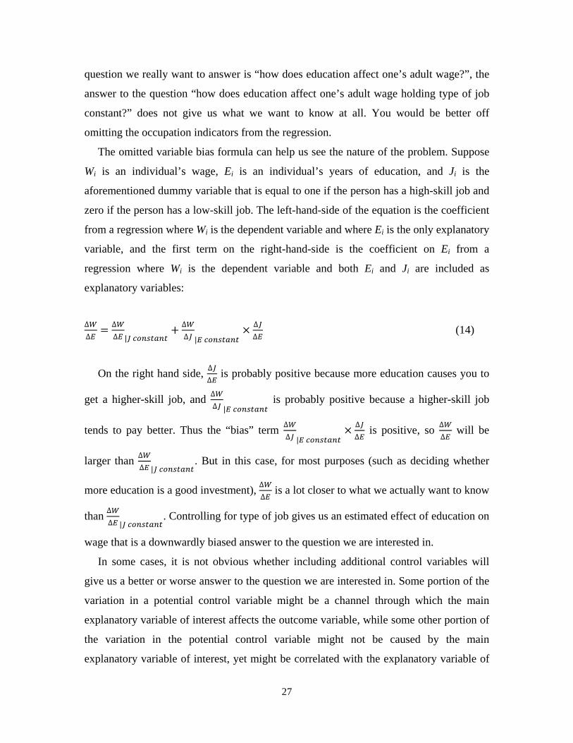
The omitted variable bias formula can help us see the nature of the problem. Suppose

Wi is an individual’s wage, Ei is an individual’s years of education, and Ji is the

aforementioned dummy variable that is equal to one if the person has a high-skill job and

zero if the person has a low-skill job. The left-hand-side of the equation is the coefficient

from a regression where Wi is the dependent variable and where Ei is the only explanatory

variable, and the first term on the right-hand-side is the coefficient on Ei from a

regression where Wi is the dependent variable and both Ei and Ji are included as

explanatory variables:

∆𝑊∆𝐸

= ∆𝑊∆𝐸 |𝐽 𝑐𝑜𝑛𝑠𝑡𝑎𝑛𝑡

+ ∆𝑊∆𝐽 |𝐸 𝑐𝑜𝑛𝑠𝑡𝑎𝑛𝑡

× ∆𝐽∆𝐸

(14)

On the right hand side, ∆𝐽∆𝐸

is probably positive because more education causes you to

get a higher-skill job, and ∆𝑊∆𝐽 |𝐸 𝑐𝑜𝑛𝑠𝑡𝑎𝑛𝑡

is probably positive because a higher-skill job

tends to pay better. Thus the “bias” term ∆𝑊∆𝐽 |𝐸 𝑐𝑜𝑛𝑠𝑡𝑎𝑛𝑡

× ∆𝐽∆𝐸

is positive, so ∆𝑊∆𝐸

will be

larger than ∆𝑊∆𝐸 |𝐽 𝑐𝑜𝑛𝑠𝑡𝑎𝑛𝑡

. But in this case, for most purposes (such as deciding whether

more education is a good investment), ∆𝑊∆𝐸

is a lot closer to what we actually want to know

than ∆𝑊∆𝐸 |𝐽 𝑐𝑜𝑛𝑠𝑡𝑎𝑛𝑡

. Controlling for type of job gives us an estimated effect of education on

wage that is a downwardly biased answer to the question we are interested in.

In some cases, it is not obvious whether including additional control variables will

give us a better or worse answer to the question we are interested in. Some portion of the

variation in a potential control variable might be a channel through which the main

explanatory variable of interest affects the outcome variable, while some other portion of

the variation in the potential control variable might not be caused by the main

explanatory variable of interest, yet might be correlated with the explanatory variable of

27

interest and might affect the outcome variable. In that case, we might get biased estimates

of the causal effect of the main explanatory variable of interest whether we include the

potential control variable or not. Including the control variable might absorb some of the

causal effect we are trying to estimate, while excluding it induces omitted variable bias.

In that case, there’s no easy solution.13

Here is an example that applies to our cross-country regression on the effects of

education on growth. Another variable that might influence economic growth, and that is

undoubtedly positively correlated with education, is quality of governance (e.g., lack of

corruption, degree of accountability and transparency in government, checks and

balances, effectiveness of government at getting things done, etc.). Suppose we had an

indicator of the quality of governance and included it as a control variable in our

regressions meant to estimate the effect of education on growth. Would that give us a

better or worse answer to the question “how does education influence economic growth?”

It is not clear. On the one hand, quality of governance might be a channel through which

education might improve growth. A more educated populace may be better able to hold

its government accountable and reduce corruption, for example because high rates of

literacy enable people to read the newspapers and stay informed about what is happening

in politics. In that case, if we controlled for quality of governance, maybe our coefficient

on education would not be giving education enough credit. On the other hand, omitting

the indicator of quality of governance is not necessarily a good solution either. Perhaps

high quality governance caused by factors other than education causes both high

educational attainment (because the education system works better when government is

more effective, competent, and uncorrupt) and also causes high growth (by improving the

security of property rights and improving incentives to invest, for example). In that case,

omitting quality of governance from the regression might give too much credit to

education for fostering growth.

Reverse Causality

In our regression analysis example above, we made growth our left-hand-side variable

and initial education our right-hand-side variable. But of course, this does not guarantee

13 King (2010) argues that this is an especially important “hard unsolved problem” in the social sciences.

28

that the direction of causality runs only from education to growth. It could well be that

faster economic growth causes people in a given country to choose to get more education,

for example because education is easier to afford when you are richer, or maybe because

peoples’ tastes change in a way that is more favorable to education as they become richer.

If growth causes education, then the coefficient on education in a regression where

growth is treated as the dependent variable might give us a very misleading impression of

the true causal effect of education on growth. Even if education had no causal effect on

growth at all, we might still estimate a positive coefficient on education because of the

reverse causality running from growth to education. That reverse causality would induce

a positive association between growth and education in the data, and the coefficient on

education would pick up that positive association. Thus, we might conclude that

education has a causal effect on growth when in fact it has no effect at all. It is just

responding to growth.

Focusing on the effect of initial education (in 1960) on subsequent growth (from 1960

through 2000) is one strategy for dealing with this problem. The hope is that something in

the past cannot be caused by something in the future. This is far from foolproof, though.

For example, growth tends to be positively correlated over time for a given country – the

countries that grow faster in one period tend to grow faster in the next period. So initial

education might have been caused by past growth, and maybe we estimate a positive

effect of initial education on subsequent growth only because past growth caused the

initial education and growth is correlated over time. Or maybe people are forward-

looking, and people who expect their country to experience high economic growth in the

future respond by investing more in education today as a result, because investments in

education pay off more when future growth is expected to be higher. In addition, for

various reasons it might make more sense to investigate the effects of changes over time

in education on growth, as opposed to the effects of initial levels of education. For

example, theoretically, it may not make so much sense to think of the level of education

at a given point in time having a permanent effect on the growth rate. But comparing

growth with changes over time in education would undoubtedly exacerbate the any

reverse causality problems. Reverse causality is always a difficult problem to solve.

29

Further study of econometrics offers some strategies which can solve the problem under

certain conditions.

Sampling Error

Sampling error is another reason why a regression estimate could provide a misleading

answer to the question we are interested in. Regression estimates are generally based on a

sample, rather than on data for an entire population. If we were to estimate our regression

over and over again on different samples randomly selected from a population, we would

get somewhat different estimates of our regression intercept and coefficients each time,

because in each sample we draw a different set of observations, each of which has a

different amount of random residual variation in the outcome variable. As a result, there

is some risk that just due to random chance, we will estimate a relationship between the

explanatory variable and the outcome variable that is very different from that in the

population, and we might even estimate a strong relationship between them when in fact

there is no systematic relationship between them in the population at all.

A simple example can illustrate the nature of the problem. Suppose we want to

estimate the average height of students in a 40-person class. We’ll treat the class as the

relevant population. If we were to estimate the height of the class by randomly selecting 5

people, measuring them, and calculating their average height, and then did this

repeatedly, we would on average get an unbiased estimate of the average height of the

class, but sometimes due to random chance we would happen to select 5 unusually tall

students and substantially overestimate the average height of the class, and on other

occasions due to random chance we would happen to select 5 unusually short students

and would substantially underestimate the average height of the class. So any particular

estimate based on a sample of 5 students could be very different from the mean height of

the population (the entire class). The smaller is the sample, the larger is the probability

that we are getting a misleading estimate of the population parameters in any particular

estimate. If we estimated the average height of the class based on just one person, there’s

a pretty high probability we’d be off by a wide margin on any given estimate, whereas if

we estimated the average height of the class based on a sample of 39 out of the 40

30

students, the probability of the estimate being very different from the population mean

would be much smaller.

The same problem applies when we estimate a regression. In our example where we

used multiple regression to examine the effects of initial education and initial income on

growth, we used a sample of 84 countries, and we used a single 40-year time period for

each country to measure growth. We can think of the relevant population here as all

possible countries and all possible time periods from the past and future. Even if we’re

really only interested in the relationship between education and growth for this particular

set of countries in this particular time period, we still have to worry about the fact that we

could be estimating a positive relationship between them due purely to random chance,

which is always possible when you have a relatively small sample size. So it is useful to

think of this in terms of sampling from a population even if the particular sample you are

investigating is of interest in and of itself. When we estimate a regression using data from

a particular sample, we get sample estimates of the various parameters in our multiple

regression equation: the intercept, the two coefficients, each country’s error term

(residual), etc. The estimated parameters in this particular sample might be very different

from the values of these parameters for the population, just due to random chance. For

example, figure 4 shows a strong positive relationship between initial education and

growth holding initial income constant. But it is at least possible that this finding is due to

random chance. Perhaps we just happened to select a sample where an unusually large

number of the countries that had high levels of initial education for their initial income

levels and also happened to have very large positive true residuals (that is, residuals

computed using the population parameters rather than the parameters estimated in this

particular sample), thus putting lots of dots in the upper-right-hand corner of figure 4. In

that case, it could be that in the population there is no systematic relationship between

initial education and growth holding initial income constant, and maybe we found a

strong relationship in our sample due to random chance.

Standard Errors, Confidence Intervals, and Statistical Significance

Fortunately, statistics provides us with ways to quantify the degree of uncertainty arising

from sampling error that is associated with each parameter of our regression model. One

31

such indicator of the degree of uncertainty arising from sampling error is the “standard

error.” Further study of statistics can teach you the details of how a standard error is

calculated and why the things I’m about to say about it are true. Here, we’ll just consider

the basic idea of what standard error means, and discuss in pragmatic terms how you can

use it to interpret the uncertainty associated with regression estimates that is due to

sampling error.

One particularly useful thing to do with a standard error for a regression coefficient is

to construct a “confidence interval.” A “95 percent confidence interval” around a

particular coefficient is a range of numbers, where the bottom of the range is the

estimated coefficient minus approximately two times the estimated standard error, and

the top of the range is the estimated coefficient plus approximately two times the

estimated standard error. To put it in symbols, when the sample is large, the 95 percent

confidence interval for a particular estimate of a coefficient 𝛽1 is approximately

[�̂�1 − 2𝑆𝐸𝛽1�, 𝛽�1 + 2𝑆𝐸𝛽1�]. A “hat” over a parameter (for example, the pointy thing on

top of �̂�1) indicates that we are talking about an estimated value of the parameter based

on this particular sample, as opposed to the “true” value of the parameter in the

population, which goes hatless. �̂�1 is our estimate of the coefficient 𝛽1 based on data

from this particular sample, and 𝑆𝐸𝛽1� is our estimate of the standard error of �̂�1 in this

particular sample. The 95% confidence interval for our estimate of 𝛽1 in this particular

sample is thus a range of numbers going from �̂�1 − 2𝑆𝐸𝛽1� to 𝛽�1 + 2𝑆𝐸𝛽1�. 14

What does the 95 percent confidence interval mean? Imagine that you could randomly

select samples from a population over and over again, and that each time you did this,

you re-estimated �̂�1 and 𝑆𝐸𝛽1� and constructed a 95 percent confidence interval using

those estimated parameters. Each time, you’d get a somewhat different estimate of the

parameters and a somewhat different confidence interval. It turns out that approximately

14 To be precise, the width of the confidence interval depends not only on the estimated coefficient and standard error, but also on the “degrees of freedom,” which is n – k – 1, where n is the number of observations in the sample, and k is the number of explanatory variables in the regression. When the degrees of freedom is greater than about 600, the 95 percent confidence interval is [�̂�1 − 1.96𝑆𝐸𝛽1�, 𝛽�1 +1.96𝑆𝐸𝛽1�]. In a regression with 84 observations and 2 explanatory variables like the one we’re considering in this article, the 95 percent confidence interval is [�̂�1 − 1.99𝑆𝐸𝛽1�, 𝛽�1 + 1.99𝑆𝐸𝛽1�]. For the purposes of this non-technical introduction, rounding to approximately two times the standard error is close enough.

32

95 percent of the times that you did this, the confidence interval you constructed would

contain the true value of the population coefficient 𝛽1. Or to put it a different way, for

any given large sample, if we conclude that the population coefficient 𝛽1 is somewhere

between �̂�1 − 2𝑆𝐸𝛽1� and 𝛽�1 + 2𝑆𝐸𝛽1� , there is about a 95 percent probability that we are

correct.

It would also be possible to construct a 90 percent confidence interval, which is

approximately [�̂�1 − (1 23)𝑆𝐸𝛽1� , 𝛽�1 + (1 2

3)𝑆𝐸𝛽1�].15 There’s nothing magical about the

use of 95 percent or 90 percent to construct the confidence intervals. Those are just

commonly-used conventions. Study of statistics teaches you how to construct confidence

intervals using whatever percentages you want.

Another useful thing you can do with a standard error is to use it to determine whether

a particular estimated coefficient is “statistically significant” in its difference from some

number (usually zero). We say that a parameter estimate is “statistically significant in its

difference from zero at the 5 percent significance level” if the estimated 95 percent

confidence interval around that estimated parameter does not include zero.16 This means

that if the true value of the population parameter were zero, there is less than a 5 percent

probability that we would have estimated a parameter as large (in absolute value) as we

did. Thus, we can be fairly confident that the population parameter involves some non-

zero effect. We say a parameter estimate is “statistically insignificant in its difference

from zero at the 5 percent significance level” if the estimated 95 percent confidence

around that estimated parameter does include zero. That simply means that if the

population value of the parameter were truly zero, there is more than a 5 percent

probability that we would estimate a parameter as large (in absolute value) as we did in a

sample of this size. Analogously, you can determine whether or not a parameter is

15 To be more precise, the 90 percent confidence interval is [�̂�1 − 1.64𝑆𝐸𝛽1�, 𝛽�1 + 1.64𝑆𝐸𝛽1�] when degrees of freedom is greater than about 600, and is [�̂�1 − 1.66𝑆𝐸𝛽1�, 𝛽�1 + 1.66𝑆𝐸𝛽1�] with the 81 degrees of freedom that we have in the main multiple regression example in this article. For our purposes, rounding to [�̂�1 − (1 2

3)𝑆𝐸𝛽1�, 𝛽�1 + (1 2

3)𝑆𝐸𝛽1�] is close enough.

16 Technically, this is for a “two-tailed test.” In some situations a “one-tailed test” might be more appropriate for the question at hand. Consult a statistics textbook for further discussion of these issues.

33

statistically significant at the 10 percent level by constructing the 90 percent confidence

interval and seeing whether or not it includes zero.

While this is not the place to go into exactly how a standard error is calculated, we can

get a rough idea of what it depends on based on the graphs shown earlier in this paper. In

figure 4, which showed the relationship between the portion of initial education that is

not predicted by initial income and the portion of growth that is not predicted by initial

income, the slope of the OLS regression line through the cloud of points gives us our

estimated �̂�1. If the cloud of points was very loosely arrayed around the regression line in

figure 4, with many points very far away from the line and many points that don’t fit the

general upward sloping pattern of the cloud, then we would tend to get a large estimated

standard error on our estimate of �̂�1. By contrast, if the cloud of points were very tightly

arrayed around the OLS regression line in figure 4, we would tend to get a smaller

estimated standard error on our estimate of �̂�1. Intuitively, when the points are tightly

arrayed around the regression line, that suggests that the true residuals are likely to be

pretty small (in absolute value) in most cases. The variation in estimates of �̂�1 from

sample to sample is caused by variation in the true residuals of the observations that

happen to be included in each sample. Other things equal, when those true residuals tend

to be smaller in absolute value, the variation in our estimates of �̂�1 from sample to sample

will be smaller, leading to less uncertainty about how far �̂�1 might be from the population

parameter, and thus a smaller standard error.

Common Misinterpretations of the Meaning of Statistical Significance

There are a number of ways to misinterpret what statistical significance means, and it is

best to get these sources of confusion out of the way early. The first is to confuse

“statistical significance” with “economic significance.” When interpreting a coefficient

estimate, we always care about at least three things: the sign of the coefficient (that is, the

estimated direction of the effect), the size of the coefficient, and the degree of uncertainty

in the estimate. “Economic significance” (also known as “social significance,” or

“importance”) is about the size of the coefficient, or in other words, it is about whether

the estimated coefficient is “big” or “small” in a meaningful economic or social sense. By

contrast, statistical significance is about the degree of uncertainty arising from sampling

34

error, and does not necessarily tell us anything about the size or importance of the effect

at all. Statistical significance and economic significance are totally different concepts,

and one does not necessarily imply the other. “Statistical significance” is a very poorly

named concept, because it actually has nothing at all to do with “significance,” which in

the English language means “importance.” This unfortunate naming convention is a

source of much confusion, but it is too late to change it now.

To take an example, in our multiple regression (equation 6), we estimated that an

additional year of initial education is associated with an annual economic growth rate

that is 0.49 percentage points higher, controlling for initial income. That is a big effect,

especially given that the mean annual growth rate was only 1.60 percent. A country that

grows at 1.6 percent per year for 40 years will be 1.89 times as rich 40 years from now as

it is today. A country that grows at 2.09 percent per year (that is 1.6 percent + 0.49

percent) for 40 years will be 2.29 times as rich 40 years from now as it is today, or 21

percent richer than it would be if it had only grown at 1.6 percent per year. That is a

substantial difference. You’d be pretty happy if your income was 21 percent higher, no?

If the standard error on that estimate was 0.1, we’d conclude that the estimate is

statistically significant at the 5 percent level, whereas if the standard error were 0.4, we

would conclude that it is not statistically significant at the 5 percent level.17 But either

way, the estimate would have the same economic significance.

If we find that an estimate is not statistically significant, we cannot conclude that the

effect is zero, and we cannot necessarily conclude that the effect is economically

unimportant either. If the confidence interval includes both zero and economically

significant effects, all we can conclude is that we are not sure whether the effect is zero

or big. We simply can’t answer the question that we set out to answer. Sometimes you

have to admit you are not sure. The only way to become less unsure about this would be

to go out and get better data that might lead to a more informative estimate with a smaller

standard error.

17 You can see this quickly by noting that an estimate will be statistically significant in its difference from zero at the 5 percent significance level if the coefficient is at least twice as large as the standard error (speaking approximately). When that is true, the 95 percent confidence interval won’t include zero.

35

In some other cases, we might be able to conclude that an estimate is economically

unimportant whether or not it is statistically significant. Suppose both of the following

two conditions are true at the same time: (1) the confidence interval is a tight band around

a very small number, and only includes economically unimportant effects; and (2) the

confidence interval does not include zero. In that case, we would call the estimate

statistically significant in its difference from zero, but we would still conclude that the

effect is economically unimportant (or “small”). Alternatively, if condition (1) above

were true, but condition (2) were not (i.e., the confidence interval does include zero), we

would call the estimate statistically insignificant, and we could also conclude that the

effect was economically insignificant as well.

The definition of “economic significance,” i.e., whether the effect is big or small,

depends on the context. You need to consider things like how the size of the effect

compares with the mean value of, and typical amount of variation in, the outcome

variable, whether a one unit change in the explanatory variable is a big change or a small

change, etc., like we did in interpreting the estimated size of the effect of initial education

on growth three paragraphs ago.

The important things to remember are that whether an estimate is statistically

significant or insignificant, by itself, does not tell us whether an effect is important, or

whether an effect is precisely zero. Rather, it just tells us something about how the degree

of uncertainty in our estimate arising from sampling error relates to the size of the

estimated coefficient.

Another common way to misinterpret statistical significance is to conclude that if you

have a statistically significant estimate, then you have a good answer to the question

you’ve asked. That may or may not be true. If you have a statistically significant

estimate, you might still have a very misleading answer to the question you are interested

in, for example because of the omitted variable bias, bad control, and/or reverse causality

problems discussed above. Standard errors only quantify the uncertainty arising from

sampling error. Standard errors don’t tell you anything at all about whether you have any

of the other problems that can make regression estimates misleading. To figure out

whether you might have those other problems, you need to think, not just apply

mechanical rules about statistical significance. A narrow confidence interval merely

36

makes us confident that our estimate is probably close to the population parameter. But

the population parameter could be a biased indicator of the causal effect we’re really

interested in. So there is no substitute for thinking critically.

How to Interpret a Table of Regression Coefficients and Standard Errors

When economics journal articles present evidence from regression analysis, they tend to

present it in a table that looks roughly like table 2 below. Typically, estimates from

different regression equations will be presented in different columns, and each column

will report estimated coefficients on each variable in different rows, with estimated

standard errors presented in parentheses under each coefficient. Table 2 follows these

conventions.18

In table 2, column (1) displays estimates from the regression of growth on initial

education from figure 1, column (2) displays estimates from the regression of growth on

initial income from figure 3, and column (3) displays estimates from our multiple

regression of growth on initial education and initial income from equation (5). Column

(4) displays estimates from a regression like that in column (3), except that landlocked,

frost area, and ethnolinguistic diversity are added as additional control variables.

Remember that each estimated coefficient represents the change in the dependent

variable associated with a one unit increase in that particular explanatory variable,

holding the other control variables constant. So to be able to interpret what each

coefficient means, you need to pay careful attention to the units of measurement for the

dependent variable and for each explanatory variable – this was discussed in connection

with table 1 above, so you might want to go back and review that now.

Focusing first on column (3), we see that the coefficient on initial education is 0.49

and the standard error on that estimate is 0.10. That coefficient means that one additional

year of initial education is associated with an annual growth rate in real GDP per worker

that is 0.49 percentage points higher, holding initial income constant. The 95 percent

confidence interval around our estimate of the effect of initial education on growth

18 Sometimes a regression table will instead report “t-statistics” in parentheses below the coefficients. A t-statistic is just the coefficient divided by the standard error. As a rough rule of thumb, a t-statistic greater than approximately 2 is indicative of an estimate that is statistically significant in its difference from zero at the 5 percent level.

37

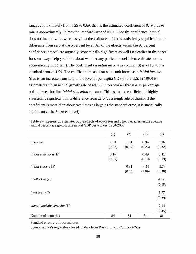
ranges approximately from 0.29 to 0.69, that is, the estimated coefficient of 0.49 plus or

minus approximately 2 times the standard error of 0.10. Since the confidence interval

does not include zero, we can say that the estimated effect is statistically significant in its

difference from zero at the 5 percent level. All of the effects within the 95 percent

confidence interval are arguably economically significant as well (see earlier in the paper

for some ways help you think about whether any particular coefficient estimate here is

economically important). The coefficient on initial income in column (3) is -4.15 with a

standard error of 1.09. The coefficient means that a one unit increase in initial income

(that is, an increase from zero to the level of per capita GDP of the U.S. in 1960) is

associated with an annual growth rate of real GDP per worker that is 4.15 percentage

points lower, holding initial education constant. This estimated coefficient is highly

statistically significant in its difference from zero (as a rough rule of thumb, if the

coefficient is more than about two times as large as the standard error, it is statistically

significant at the 5 percent level).

Table 2 -- Regression estimates of the effects of education and other variables on the average annual percentage growth rate in real GDP per worker, 1960-2000

(1) (2) (3) (4)

intercept 1.00 1.51 0.94 0.96

(0.27) (0.24) (0.25) (0.32)

initial education (E) 0.16

0.49 0.41

(0.06)

(0.10) (0.09)

initial income (Y)

0.31 -4.15 -5.74

(0.64) (1.09) (0.99)

landlocked (L)

-0.65

(0.35)

frost area (F)

1.97

(0.39)

ethnolinguistic diversity (D)

0.04 (0.45) Number of countries 84 84 84 81

Standard errors are in parentheses. Source: author's regressions based on data from Bosworth and Collins (2003).

38

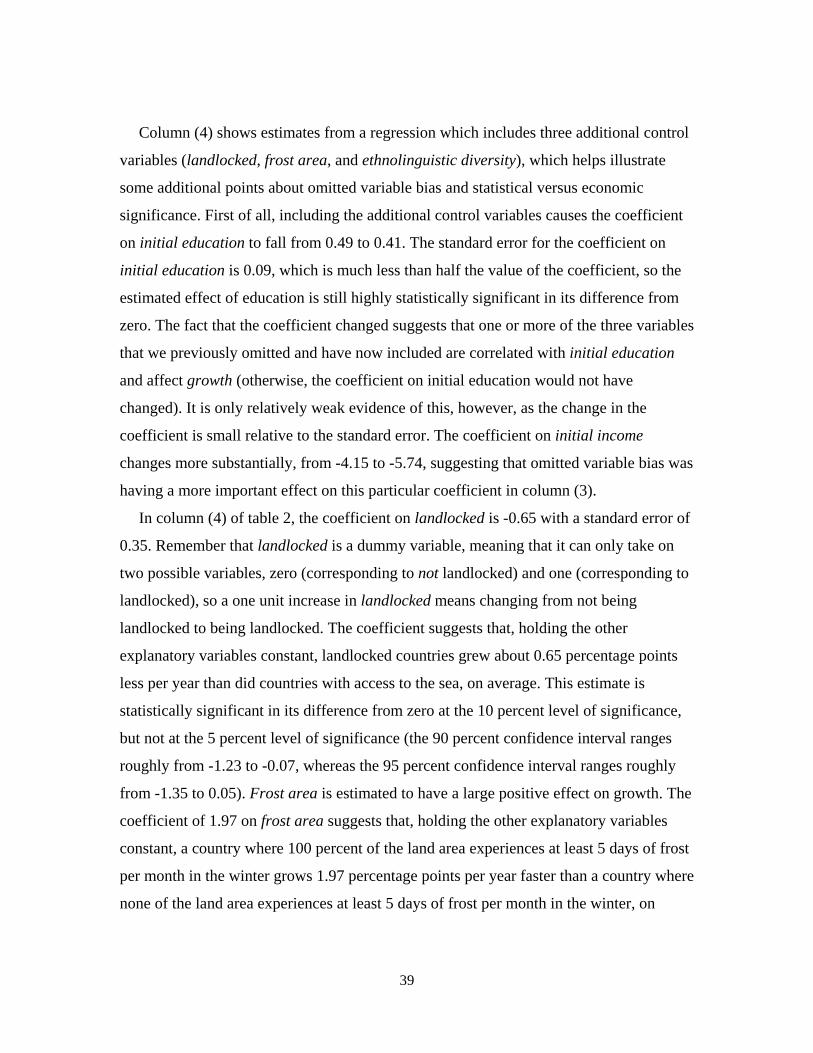
Column (4) shows estimates from a regression which includes three additional control

variables (landlocked, frost area, and ethnolinguistic diversity), which helps illustrate

some additional points about omitted variable bias and statistical versus economic

significance. First of all, including the additional control variables causes the coefficient

on initial education to fall from 0.49 to 0.41. The standard error for the coefficient on

initial education is 0.09, which is much less than half the value of the coefficient, so the

estimated effect of education is still highly statistically significant in its difference from

zero. The fact that the coefficient changed suggests that one or more of the three variables

that we previously omitted and have now included are correlated with initial education

and affect growth (otherwise, the coefficient on initial education would not have

changed). It is only relatively weak evidence of this, however, as the change in the

coefficient is small relative to the standard error. The coefficient on initial income

changes more substantially, from -4.15 to -5.74, suggesting that omitted variable bias was

having a more important effect on this particular coefficient in column (3).

In column (4) of table 2, the coefficient on landlocked is -0.65 with a standard error of

0.35. Remember that landlocked is a dummy variable, meaning that it can only take on

two possible variables, zero (corresponding to not landlocked) and one (corresponding to

landlocked), so a one unit increase in landlocked means changing from not being

landlocked to being landlocked. The coefficient suggests that, holding the other

explanatory variables constant, landlocked countries grew about 0.65 percentage points

less per year than did countries with access to the sea, on average. This estimate is

statistically significant in its difference from zero at the 10 percent level of significance,

but not at the 5 percent level of significance (the 90 percent confidence interval ranges

roughly from -1.23 to -0.07, whereas the 95 percent confidence interval ranges roughly

from -1.35 to 0.05). Frost area is estimated to have a large positive effect on growth. The

coefficient of 1.97 on frost area suggests that, holding the other explanatory variables

constant, a country where 100 percent of the land area experiences at least 5 days of frost

per month in the winter grows 1.97 percentage points per year faster than a country where

none of the land area experiences at least 5 days of frost per month in the winter, on

39

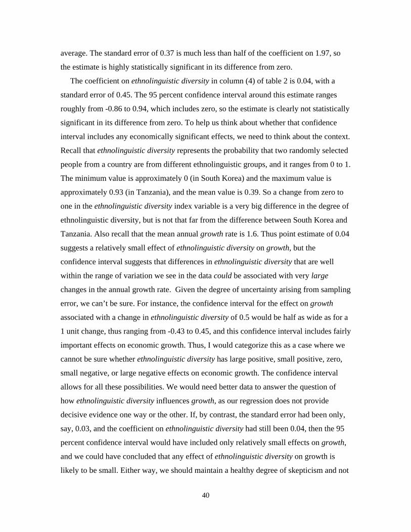
average. The standard error of 0.37 is much less than half of the coefficient on 1.97, so

the estimate is highly statistically significant in its difference from zero.

The coefficient on ethnolinguistic diversity in column (4) of table 2 is 0.04, with a

standard error of 0.45. The 95 percent confidence interval around this estimate ranges

roughly from -0.86 to 0.94, which includes zero, so the estimate is clearly not statistically

significant in its difference from zero. To help us think about whether that confidence

interval includes any economically significant effects, we need to think about the context.

Recall that ethnolinguistic diversity represents the probability that two randomly selected

people from a country are from different ethnolinguistic groups, and it ranges from 0 to 1.

The minimum value is approximately 0 (in South Korea) and the maximum value is

approximately 0.93 (in Tanzania), and the mean value is 0.39. So a change from zero to

one in the ethnolinguistic diversity index variable is a very big difference in the degree of

ethnolinguistic diversity, but is not that far from the difference between South Korea and

Tanzania. Also recall that the mean annual growth rate is 1.6. Thus point estimate of 0.04

suggests a relatively small effect of ethnolinguistic diversity on growth, but the

confidence interval suggests that differences in ethnolinguistic diversity that are well

within the range of variation we see in the data could be associated with very large

changes in the annual growth rate. Given the degree of uncertainty arising from sampling

error, we can’t be sure. For instance, the confidence interval for the effect on growth

associated with a change in ethnolinguistic diversity of 0.5 would be half as wide as for a

1 unit change, thus ranging from -0.43 to 0.45, and this confidence interval includes fairly

important effects on economic growth. Thus, I would categorize this as a case where we

cannot be sure whether ethnolinguistic diversity has large positive, small positive, zero,

small negative, or large negative effects on economic growth. The confidence interval

allows for all these possibilities. We would need better data to answer the question of

how ethnolinguistic diversity influences growth, as our regression does not provide

decisive evidence one way or the other. If, by contrast, the standard error had been only,

say, 0.03, and the coefficient on ethnolinguistic diversity had still been 0.04, then the 95

percent confidence interval would have included only relatively small effects on growth,

and we could have concluded that any effect of ethnolinguistic diversity on growth is

likely to be small. Either way, we should maintain a healthy degree of skepticism and not

40

be too confident in our estimates, given all the other ways that a regression analysis can

go wrong, such as omitted variable bias, reverse causality, and bad control, among other

things.

Conclusion

There is of course plenty more to learn about regression analysis and econometrics.

Further study can give you a deeper, more mathematical understanding of the issues

discussed here, including demonstrations for why some of the claims made here are true,

and it can teach you about various clever strategies for addressing some of the challenges

and problems raised above. My hope is that this paper has made the basic idea of

regression analysis reasonably transparent, that it has equipped you to read, understand,

interpret, and think critically about papers involving multiple regression analyses, and

that it has inspired you to want to learn more.

41

References Angrist, Joshua D., and Jorn-Steffen Pischke. 2009. Mostly Harmless Econometrics: An Empiricist's Companion. Princeton and Oxford: Princeton University Press. Bosworth, Barry P., and Susan M. Collins. 2003. "The Empirics of Growth: An Update." Brookings Papers on Economic Activity. No. 2, pp. 113-179. Department of Geodesy and Cartography of the State Geological Committee of the USSR. 1964. Atlas Narodov Mira. Moscow. Easterly, William, and Ross Levine. 1997. “Africa’s Growth Tragedy: Policies and Ethnic Divisions.” Quarterly Journal of Economics. Vol. 112, No. 3, pp. 1203–50. Eberhardt, Markus, and Francis Teal. 2011. "Econometrics for Grumblers: A New Look at the Literature on Cross-Country Growth Empirics." Journal Of Economic Surveys. Vol. 25, No. 1, pp. 109-155. Gallup, John Luke, Jeffrey D. Sachs, and Andrew D. Mellinger. 1999. "Geography and Economic Development." In Annual World Bank Conference on Development Economics, 1998. Washington, D.C.: World Bank, pp. 127-178 Frisch, Ragnar and Frederick V. Waugh. 1933. “Partial Time Regression as Compared with Individual Trends.” Econometrica. Vol. 1, pp. 387-401. King, Gary. 2010. “A Hard Unsolved Problem? Post-Treatment Bias in Big Social Science Questions.” Slides from a talk given at Harvard University, April 10. <http://gking.harvard.edu/talks/bigprobP.pdf> (accessed August 29, 2012). Masters, William A., and Margaret S. McMillan. 2001. “Climate and Scale in Economic Growth.” Journal of Economic Growth. Vol. 6, No. 3, pp. 167–86. Mauro, Paolo. 1995. "Corruption and Growth." Quarterly Journal of Economics. Vol. 110, No. 3, pp. 681-712. Rodrik, Dani, Arvind Subramanian, and Francesco Trebbi. 2004. "Institutions Rule: The Primacy of Institutions over Geography and Integration in Economic Development." Journal of Economic Growth. 9, no. 2: 131-165. Solow, Robert M. 1957. "Technical Change and the Aggregate Production Function." Review of Economics and Statistics. Vol. 39, pp. 312-320. Stock, James and Mark Watson. 2007. Introduction to Econometrics, 2nd ed. Boston: Pearson Education. Wheelan, Charles. 2013. Naked Statistics. New York: W.W. Norton.

42