A Nonparametric Bayesian Approach Towards Robot Learning by … · 2014-06-01 · A Nonparametric Bayesian Approach Towards Robot Learning by Demonstration Sotirios P. Chatzis, Dimitrios

A Nonparametric Bayesian Approach Towards Robot

Learning by Demonstration

Sotirios P. Chatzis, Dimitrios Korkinof, and Yiannis Demiris

Abstract

In the last years, many authors have considered application of machine learn-ing methodologies to effect robot learning by demonstration. Gaussian mixtureregression (GMR) is one of the most successful methodologies used for this pur-pose. A major limitation of GMR models concerns automatic selection of theproper number of model states, i.e. the number of model component densities.Existing methods, including likelihood- or entropy-based criteria, usually tendto yield noisy model size estimates while imposing heavy computational require-ments. Recently, Dirichlet process (infinite) mixture models have emerged inthe cornerstone of nonparametric Bayesian statistics as promising candidates forclustering applications where the number of clusters is unknown a priori. Underthis motivation, to resolve the aforementioned issues of GMR-based methods forrobot learning by demonstration, in this paper we introduce a nonparametricBayesian formulation for the GMR model, the Dirichlet process GMR model.We derive an efficient variational Bayesian inference algorithm for the proposedmodel, and we experimentally investigate its efficacy as a robot learning bydemonstration methodology, considering a number of demanding robot learningby demonstration scenarios.

Keywords: Gaussian mixture regression, robot learning by demonstration,Dirichlet process, variational Bayes, nonparametric statistics.

1. Introduction

In the last years, robot learning by demonstration has turned out to be oneof the most active research topics in the field of robotics. Robot learning bydemonstration encompasses methods by which a robot can learn new skills bysimple observation of a human teacher, similar to the way humans learn newskills by imitation (author?) [1, 2, 3, 4, 5, 6, 7, 10]. Coming up with successfulrobot learning by demonstration methodologies can be of great benefit to therobotics community, since it will greatly obviate the need of programming arobot how to perform a task, which can be rather tedious and expensive, while,by making robots more user-friendly, it increases the appeal of applying robotsto real-life environments.

Towards this end, robotics researchers have utilized a multitude of method-ologies from as diverse research areas as machine learning, computer vision

Preprint submitted to Elsevier February 3, 2012

Robotics and Autonomous Systems, vol. 60:6, pp. 789-802, June 2012

[8], and human-robot interaction [45]. Learning by demonstration algorithmsmay comprise learning an approximation to the state-action mapping (map-ping function), or learning a model of the world dynamics and deriving a policyfrom this information (system model). Mapping function learning comprisesclassification-based and regression-based approaches. Classification approachescategorize their input into discrete classes, thus the input to the classifier is therobot state, and the discrete output classes are robot actions. Gaussian Mix-ture Models (GMMs), decision trees, Bayesian networks, and hidden Markovmodels are typical methods used to effect the classification task. Regression ap-proaches map demonstration states to continuous action spaces resulting fromcombining multiple demonstration set actions. As such, typically regressionapproaches apply to low-level trajectory-based learning by demonstration, andnot to high-level behaviors. Finally, the system model approach uses a statetransition model of the world, and from this derives a policy, typically by meansof reinforcement learning (RL). As such, it usually has the drawback of highcomputational demands, due to the considerably large dimensionality of theentailed search space of the RL algorithm.

In this work, we focus on trajectory-based learning by demonstration tech-niques. Two of the most popular trends of work in this field consist in theinvestigation of the utility of probabilistic generative models, such as Gaussianmixture regression (GMR) and derivatives, [15] hidden Markov models [16], andGaussian process regression (author?) [2]. GMR, in particular, has been shownto be very successful in encoding demonstrations, extracting their underlyingconstraints, and reproducing smooth generalized motor trajectories, while im-posing considerably low computational costs [18, 1]. GMR-based approachestowards learning by demonstration rely on the postulation of a Gaussian mix-ture model to encode the covariance relations between different variables (eitherin the task space, or in the robot joints space). If the correlations vary signifi-cantly between regions, then each local region of the state space visited duringthe demonstrations will need a few Gaussians to encode these local dynamics.Given the required number of Gaussians and a set of training data (human-generated demonstrations), the expectation-maximization (EM) algorithm iseventually employed to estimate the parameters of the model.

The most common data-driven methodologies for GMR model selection, thatis determination of the appropriate number of GMR model component densities,are typically based on the popular Bayesian information criterion (BIC) for fi-nite mixture models [19], or other related likelihood-based or entropy-basedmodel size selection criteria [20]. However, such model selection methods suf-fer from significant drawbacks: To begin with, they entail training of multiplemodels (to select from), a tedious procedure which can be applied only up toa limited extent, due to its computational demands. Moreover, effectivenessof the BIC criterion is contingent on a number of conditions, which are notnecessarily fulfilled in real-life application scenarios [20]; thus, BIC-based ap-proximations are rather prone to yielding noisy model size estimates. Mostsignificantly, likelihood- and entropy-based model selection criteria are notori-ous for their heavy overfitting proneness, hence often leading to over-estimation

2


of the required model size [22].Dirichlet process mixture (DPM) models are flexible Bayesian nonparamet-

ric models which have become very popular in statistics over the last few years,for performing nonparametric density estimation [23, 24, 25]. Briefly, a realiza-tion of a DPM can be seen as an infinite mixture of distributions with givenparametric shape (e.g., Gaussian). This theory is based on the observation thatan infinite number of component distributions in an ordinary finite mixturemodel tends on the limit to a Dirichlet process prior [24, 26]. Indeed, althoughtheoretically a DPM model has an infinite number of parameters, it turns outthat inference for the model is possible, since only the parameters of a finitenumber of mixture components need to be represented explicitly; this can bedone by means of an elegant and computationally efficient truncated variationalBayesian approximation [28]. Eventually, as a part of the model fitting proce-dure, the nonparametric Bayesian inference scheme induced by a DPM modelyields a posterior distribution on the proper number of model component den-sities [29], rather than selecting a fixed number of mixture components. Hence,the obtained nonparametric Bayesian formulation eliminates the need of doinginference (or making arbitrary choices) on the number of mixture componentsnecessary to represent the modeled data.

Under this motivation, in this work we introduce a nonparametric Bayesianapproach towards Gaussian mixture regression, with application to robot learn-ing by demonstration. Our approach is based on the consideration of a GMRmodel with a countably infinite number of constituent states, and is effected byutilization of a Dirichlet process (DP) prior distribution; we shall be referring tothis new model as the Dirichlet process Gaussian mixture regression (DPGMR)model. Inference for the DPGMR model is conducted using an elegant varia-tional Bayesian algorithm, and is facilitated by means of a stick-breaking con-struction of the DP prior, which allows for the derivation of a computationallytractable expression of the model variational posteriors. Our novel mixture re-gression methodology is subsequently applied to yield a nonparametric Bayesianapproach towards robot learning by demonstration, the efficacy of which is illus-trated by considering a number of demanding robot learning by demonstrationscenarios.

The remainder of this paper is organized as follows: In Section 2, Gaussianmixture regression as applied to robot learning by demonstration is introducedin a concise manner. In Section 3, we provide a brief review of concepts fromthe field of Dirichlet process mixture models, emerging in the cornerstone ofnonparametric Bayesian statistics. In Section 4, we derive the proposed non-parametric Bayesian approach towards robot learning by demonstration. InSection 5, the experimental evaluation of the proposed algorithm is performed.The final section concludes this paper.

3


2. Gaussian Mixture Regression for Robot Learning by Demonstra-tion

Let us consider the current position of the moving end-effector of a robotas the predictor variable β of our machine learning algorithm, and the velocitythat must be adopted by the robot’s end-effector at the next time-step, in orderto comply with the learnt trajectory, as the algorithm’s response variable β.GMR postulates a model of the conditional expectation of the set of responsevariables β given the set of predictor variables β, by exploiting the informationavailable in a set of training observations {βj , βj}Nj=1.

A significant advantage of GMR-based methodologies is that, contrary tomost traditional regression methodologies, GMR does not directly approximatethe regression function but postulates a GMM to model the joint probabilitydistribution of the considered response and predictor variables (β and β), i.e.it considers a model of the form

p(β, β|π, {µi,Σi}Ki=1) =

K∑

i=1

πiN (β, β|µi,Σi) (1)

where π = (πi)Ki=1 are the prior weights of the mixture component densities,

and N (·|µi,Σi) is a Gaussian with mean µi and covariance matrix Σi. As aresult, contrary to most discriminative regression algorithms (e.g., SVMs [31],and Gaussian processes [32]), the computational time required for trajectoryreproduction does not increase with the number of demonstrations provided tothe robot, which is a particularly important property for lifelong learning robots.Indeed, the available model training data provided by the employed humandemonstrators is processed in only an off-line fashion, to obtain the estimates ofthe model parameters. This way, prediction generation under GMR reduces to asimple weighted sum of linear models, which is advantageous because trajectoryreproduction becomes fast enough to be used at any appropriate time by therobot.

The GMM (1) postulated under the GMR approach is trained by means ofthe EM algorithm [20], using a set of training data corresponding to a numberof trajectories obtained by human demonstrators. Then, using the obtainedGMM p(β, β|π, {µi,Σi}Ki=1), Gaussian mixture regression retrieves a gener-alized trajectory by estimating at each time step the conditional expectation

E

[β|β;π, {µi,Σi}Ki=1

]. Expressing the means µi of the component densities of

the postulated GMM (1) in the form

µi =

[µβi

µβi

](2)

and introducing the notation

Σi =

[Σ

βi Σ

ββi

Σββi Σ

βi

](3)

4


for the covariance matrices of the model component densities, we can showthat, based on (1) and the assumptions (2)-(3), the conditional probability

p(β|β;π, {µi,Σi}Ki=1

)of the response variables β given the predictor variables

β and the postulated GMM yields [30]

p(β|β;π, {µi,Σi}Ki=1

)= N (β|µ, Σ) (4)

where

µ =

K∑

i=1

φi(β)

[µ

βi +Σ

ββi

(Σ

βi

)−1

(β − µβi )

](5)

Σ =

K∑

i=1

φ2i (β)

[Σ

βi −Σ

ββi

(Σ

βi

)−1

Σββi

](6)

and

φi(β) =πiN (β|µβ

i ,Σβi )∑K

k=1 πkN (β|µβk ,Σ

βk )

(7)

Based on the result (4), predictions under the GMR approach can be obtained

by taking the conditional expectations E

(β|β;π, {µi,Σi}Ki=1

), i.e.

β = E


)= µ (8)

As we observe, a significant merit of GMR consists in the fact that it providesa full predictive distribution, thus a predictive variance

V


)= Σ

is available at any position of the end-effector. Therefore, GMR offers a model-estimated measure of predictive uncertainty not only at specific positions butcontinuously along the generated trajectories.

Data-driven selection of the appropriate number of GMR states (model com-ponent densities) is a crucial procedure for successfully applying GMR-basedrobot learning by demonstration: The number of postulated GMR states de-termines the compromise between accuracy and smoothness of the obtainedresponse (bias-variance tradeoff). Optimal model size (order) selection for fi-nite mixture models is an important but very difficult problem which has notbeen completely resolved. Usually, penalized likelihood-based or entropy-basedcriteria are used for this purpose [20], such as the Bayesian information criterion(BIC) of Schwarz [19], and variants [22].

The BIC model selection criterion as applied to a GMR-fitted GMM used fortrajectory-based robot learning by demonstration consists in the determinationof the number of model component densities which minimizes the metric

L , −2N∑

n=1

logp({βn, βn}Nn=1|π, {µi,Σi}Ki=1

)+ dlogN (9)

5


where d is the total number of model parameters, hence a function of the numberof mixture component densities K, and N is the number of available modeltraining data points. BIC has been shown to provide consistent model orderestimators under certain conditions [33]. However, these conditions are notnecessarily fulfilled in real-world application scenarios [20]. Additionally, BIChas been found to fit too few components when the model for the componentdensities (here, the Gaussian assumption) is valid and the sample size is not verylarge [34]. Finally, if the model for the component densities is not valid, thenit has been found to fit too many components [20]. This is the most commonissue that plagues GMR when it comes to its robot learning by demonstrationapplications, since it is a problem practitioners are quite often confronted with,and it may severely undermine the performance of the GMR-based learning bydemonstration algorithm, by giving rise to overfitting issues.

The main aim of this work is to resolve these very issues of GMR-basedrobot learning by demonstration, by coming up with a method that allows forautomatic, data-driven determination of the proper number of model componentdensities K, without being vulnerable to overfitting.

3. Dirichlet process mixture models

Dirichlet process models were first introduced by Ferguson [35]. A DP ischaracterized by a base distribution G0 and a positive scalar α, usually referredto as the innovation parameter, and is denoted as DP(G0, α). Essentially, a DPis a distribution placed over a distribution. Let us suppose we randomly drawa sample distribution G from a DP, and, subsequently, we independently drawN random variables {Θ∗

n}Nn=1 from G:

G|{G0, α} ∼ DP(G0, α) (10)

Θ∗

n|G ∼ G, n = 1, . . .N (11)

Integrating out G, the joint distribution of the variables {Θ∗

n}Nn=1 can be shownto exhibit a clustering effect. Specifically, given the first N − 1 samples of G,{Θ∗

n}N−1n=1 , it can be shown that a new sample Θ∗

N is either (a) drawn from thebase distribution G0 with probability α

α+N−1 , or (b) is selected from the existingdraws, according to a multinomial allocation, with probabilities proportional tothe number of the previous draws with the same allocation [36]. Let {Θc}Kc=1

be the set of distinct values taken by the variables {Θ∗

n}N−1n=1 . Denoting as fN−1

c

the number of values in {Θ∗

n}N−1n=1 that equal to Θc, the distribution of Θ∗

N given{Θ∗

n}N−1n=1 can be shown to be of the form [36]

p(Θ∗

N |{Θ∗

n}N−1n=1 , G0, α) =

α

α+N − 1G0

+

K∑

c=1

fN−1c

α+N − 1δΘc

(12)

6


where δΘcdenotes the distribution concentrated at a single point Θc. These

results illustrate two key properties of the DP scheme. First, the innovationparameter α plays a key-role in determining the number of distinct parametervalues. A larger α induces a higher tendency of drawing new parameters fromthe base distribution G0; indeed, as α → ∞ we get G → G0. On the contrary,as α → 0 all {Θn}Nn=1 tend to cluster to a single random variable. Second, themore often a parameter is shared, the more likely it will be shared in the future.

A characterization of the (unconditional) distribution of the random variableG drawn from a Dirichlet process DP(G0, α) is provided by the stick-breakingconstruction of Sethuraman [28]. Consider two infinite collections of indepen-dent random variables v = (vc)

∞

c=1, {Θc}∞c=1, where the vc are drawn from theBeta distribution Beta(1, α), and the Θc are independently drawn from the basedistribution G0. The stick-breaking representation of G is then given by [28]

G =

∞∑

c=1

πc(v)δΘc(13)

where

πc(v) = vc

c−1∏

j=1

(1− vj) ∈ [0, 1] (14)

and∞∑

c=1

πc(v) = 1 (15)

The stick-breaking representation of the DP makes clear that the random vari-able G drawn from a DP is discrete. It shows explicitly that the support of Gconsists of a countably infinite sum of atoms located at Θc, drawn independentlyfrom G0. It is also apparent that the innovation parameter α controls the meanvalue of the stick variables, vc, as a hyperparameter of their prior distribution;hence, it regulates the effective number of the distinct values of the drawn atoms[28].

Under the stick-breaking representation (13) of the Dirichlet process, theatoms Θc, drawn independently from the base distribution G0, can be seen asthe parameters of the component distributions of a mixture model comprisingan unbounded number of component densities, with mixing proportions πc(v).This way, DP mixture (DPM) models are formulated [26].

Let y = {yn}Nn=1 be a set of observations modeled by a DPM model. Then,each one of the observations yn is assumed to be drawn from its own probabilitydensity function p(yn|Θ∗

n) parametrized by the parameter set Θ∗

n. All Θ∗

n followa common DP prior, and given the discreteness of G, may share the same valueΘc with probability πc(v). Introducing the indicator variables x = (xn)

Nn=1,

with xn = c denoting that Θ∗

n takes on the value of Θc, the modeled data set ycan be described as arising from the process

yn|xn = c; Θc ∼ p(yn|Θc) (16)

7


xn|π(v) ∼ Mult(π(v)) (17)

vc|α ∼ Beta(1, α) (18)

Θc|G0 ∼ G0 (c = 1, ..,∞) (19)

where π(v) = (πc(v))∞

c=1 is given by (14), and Mult(π(v)) is a Multinomialdistribution over π(v).

4. Proposed Approach

Let y = {yn}Nn=1, with yn = {βn, βn} being the set of predictor variablesand response variables the joint distribution of which is represented by means ofa postulated GMR model. We want to model this data by means of a nonpara-metric Bayesian formulation of the GMR model. For this purpose, we postulatea GMR model with a countably infinite number of states. To formulate such amodel, we begin by postulating a Gaussian DPM model for the joint distribu-tion of the β and β, and we further derive the expressions for the conditionalpredictive distribution of the response variables β given the predictor variablesβ.

Denoting as x = (xn)Nn=1 the labels of the GMR states emitting the fitting

data y, we haveyn|xn = c; Θc ∼ N (µc,Rc) (20)

for the state-conditional likelihoods of the model, where Θc = {µc,Rc}, andN (µc,Rc) is a Gaussian distribution with mean µc and precision (inverse co-variance) Rc, while it holds

p(x) =N∏

n=1

p(xn|π(v)) (21)

with the p(xn = c|π(v)) being the prior probabilities of the model states, stem-ming from the imposed Dirichlet process, given by (14) and (17).

Definition. We denote as the Dirichlet process Gaussian mixture regression(DPGMR) model a Gaussian mixture regression model with a countably infinitenumber of states, based on the introduction of a Dirichlet process as the priorof its state emission probabilities.

4.1. Inference for the DPGMR model

Inference for DPM-type models can be conducted under a Bayesian setting,typically by means of variational Bayes (e.g., [37]), or Monte Carlo techniques(e.g., [38]). Here, we prefer a variational Bayesian approach, due to its con-siderably better scalability in terms of computational costs. Bayesian inferenceinvolves introduction of a set of appropriate priors over the model parame-ters, and derivation of the corresponding (approximate) posterior densities. We

8


choose conjugate-exponential priors, as this selection greatly simplifies inferenceand interpretability [30]. Hence, we impose a joint Normal-Wishart distributionover the means and precisions of the Gaussian likelihoods of the model states

p(Θc) = NW(µc,Rc|λc,mc, ω,Ψc) (22)

We mention that in (22) we have assumed a common value for the hyperpa-rameters ω of the model component densities, i.e., ωc = ωc′ = ω, ∀c 6= c′.We make this hyperparameter tying assumption so as to simplify the resultingexpression of the model predictive density, derived in Section 4.2. Additionally,taking under consideration the effect of the innovation hyperparameter α onthe number of effective component densities (states) of a DPM-type model, wechoose to also impose a (hyper-)prior over the innovation hyperparameter α ofthe DPGMR model. We use a Gamma prior with

p(α) = G(α|γ1, γ2). (23)

Our variational Bayesian inference formalism for the DPGMR model con-sists in derivation of a family of variational posterior distributions q(.) whichapproximate the true posterior distribution over the infinite sets v = (vc)

∞

c=1

and {µc,Rc}∞c=1, and the innovation parameter α. Apparently, under this in-finite dimensional setting, Bayesian inference is not tractable. For this reason,we employ a common strategy in DPM literature, formulated on the basis of atruncated stick-breaking representation of the DP [37]. That is, we fix a value Kand we let the variational posterior over the vi have the property q(vK = 1) = 1.In other words, we set πc(v) equal to zero for c > K. Note that, under thissetting, the treated DPGMR model involves a full DP prior; truncation is notimposed on the model itself, but only on the variational distribution to allow fora tractable inference procedure. Hence, the truncation level K is a variationalparameter which can be freely set, and not part of the prior model specification.

Let W = {v, α,x,µc,Rc}Kc=1 be the set of hidden variables and unknownparameters of the DPGMR model over which a prior distribution has been im-posed, and Ξ be the set of the hyperparameters of the imposed priors, Ξ ={λc,mc, ω,Ψc, γ1, γ2}Kc=1. Variational Bayesian inference consists in the intro-duction of an arbitrary distribution q(W ) to approximate the actual posteriorp(W |Ξ,y), which is computationally intractable [30]. Under this assumption,the log marginal likelihood (log evidence), logp(y), of the model yields [39]

logp(y) = L(q) + KL(q||p) (24)

where

L(q) =ˆ

dWq(W )logp(y,W |Ξ)q(W )

(25)

and KL(q||p) stands for the Kullback-Leibler (KL) divergence between the (ap-proximate) variational posterior, q(W ), and the actual posterior, p(W |Ξ,y).Since KL divergence is nonnegative, L(q) forms a strict lower bound of the logevidence, and would become exact if q(W ) = p(W |Ξ,y). Hence, by maximizing

9


this lower bound L(q) (variational free energy) so that it becomes as tight aspossible, not only do we minimize the KL-divergence between the true and thevariational posterior, but we also implicitly integrate out the unknowns W .

Due to the considered conjugate prior configuration of the DPGMR model,the variational posterior q(W ) is expected to take the same functional form asthe prior, p(W ) [22]; thus, it is expected to factorize as

q(W ) =q(x)q(α)

(K−1∏

c=1

q(vc)

)K∏

c=1

q (µc,Rc) (26)

with

q(x) =

N∏

n=1

q(xn) (27)

Then, the variational free energy of the model reads (ignoring constant terms)

L(q) =K∑

c=1

ˆ

dRc

ˆ

dµc

[q(µc,Rc)

× logp(µc,Rc|λc,mc, ω,Ψc)

q(µc,Rc)

]

+

ˆ

dαq(α)

{log

p(α|γ1, γ2)q(α)

+

K−1∑

c=1

ˆ

dvcq(vc)logp(vc|α)q(vc)

}

+

K∑

c=1

N∑

n=1

q(xn = c)

{ˆ

dvq(v)logp(xn = c|π(v))q(xn = c)

+

ˆ

dRc

ˆ

dµcq(µc,Rc)logp(yn|Θc)

}

(28)

The analytical expression of the variational free energy L(q) can be found inthe Appendix.

Derivation of the variational posterior distribution q(W ) involves maximiza-tion of the variational free energy L(q) over each one of the factors of q(W ) inturn, holding the others fixed, in an iterative manner [40]. By construction, thisiterative, consecutive updating of the variational posterior distribution is guar-anteed to monotonically and maximally increase the free energy L(q), whichfunctions as the convergence criterion of the derived inference algorithm for theDPGMR model [22].

Let us denote as 〈.〉 the posterior expectation of a quantity. We begin withthe posterior distributions over the DP parameters. From (28), we have

q(vc) = Beta(ηc,1, ηc,2) (29)

10


where

ηc,1 = 1 +

N∑

n=1

q(xn = c) (30)

ηc,2 = 〈α〉+K∑

c′=c+1

N∑

n=1

q(xn = c′) (31)

andq(α) = G(α|γ1, γ2) (32)

whereγ1 = γ1 +K − 1 (33)

γ2 = γ2 −K−1∑

c=1

[ψ(ηc,2)− ψ(ηc,1 + ηc,2)] (34)

and ψ(.) denotes the Digamma function.Similar, regarding the posteriors over the likelihood parameters, we have

q(Θc) = q(µc,Rc) = NW(µc,Rc|λc, mc, ω, Ψc) (35)

where we introduce the notation

γc ,

N∑

n=1

q(xn = c) (36)

yc ,

∑Nn=1 q(xn = c)yn

γc(37)

∆c ,

N∑

n=1

q(xn = c) (yn − yc) (yn − yc)T

(38)

and, we have

ω = ω + 1 +1

K

K∑

c=1

γc (39)

Ψc = Ψc +∆c +λcγcλc + γc

(mc − yc) (mc − yc)T

(40)

λc = λc + γc (41)

mc =λcmc + γcyc

λc(42)

Finally, the posteriors over the model states generating the data yield

q(xn = c) ∝ πc(v)p(yn|Θc) (43)

11


where

πc(v) , exp (〈logπc(v)〉)

= exp

[c−1∑

c′=1

〈log(1 − vc′)〉+ 〈logvc〉]

(44)

and

p(yn|Θc) ,exp (〈logp(yn|Θc)〉)

=exp

[− d

2log2π +

1

2〈log |Rc|〉

− 1

2

⟨(yn − µc)

TRc (yn − µc)

⟩ ](45)

The expressions of the posterior expected values included in the update equa-tions (29)-(45) can be found in the Appendix.

4.2. Predictive Density

Having obtained the (variational) Bayesian estimators of the DPGMR modelparameters, we can now proceed to the derivation of the model predictive den-

sity, that is the conditional density p(β|β;y

), where y is the training set used

for model estimation.Let us first consider the expression of the joint predictive density p

(β, β|y

)

of our model. Based on the formulation of the Gaussian DPM employed by ourmodel, we have

p(β, β|y

)=

ˆ

dvq(v)

K∑

c=1

p(x = c|π(v))

×ˆ

dµc

ˆ

dRcq(µc,Rc)p(β, β|x = c;µc,Rc)

(46)

which yields a Student’s-t predictive density of the form [30]

p(β, β|y

)=

K∑

c=1

〈πc(v)〉St(β, β|mc,Sc, ω + 1− d) (47)

where d is the total dimensionality of the modeled input space {β, β}, mc isgiven by (42), and the covariance matrix of the predictive density Sc yields

Sc =1 + λc

(ω + 1− d)λcΨc (48)

while the expression of the posterior expectations 〈πc(v)〉 can be found in theAppendix.

12


Having obtained the expression of the predictive density p(β, β|y

), shown

to be of a Student’s-t form, we can now proceed to the derivation of the condi-

tional predictive density p(β|β;y

)of the response variables β given the predic-

tor variables β. Let us consider the state-conditional expression of the predictivedistribution (47). Setting

mc =

[mβ

c

mβc

](49)

and

Sc =

[Sβ

c Sββc

Sββc Sβ

c

](50)

we can write

[β

β

]|x = c;y ∼ St

([mβ

c

mβc

],

[Sβ

c Sββc

Sββc Sβ

c

], ω + 1− d

)(51)

wherep(x = c) = 〈πc(v)〉 (52)

As discussed, e.g., in [22], the Student’s-t distribution can be equivalentlywritten as an infinite sum of Gaussians with the same means and scaled covari-ances, where the covariance scalars are Gamma-distributed latent variables:

St(x|µ,Σ, ν) =ˆ

∞

0

N (x|µ, 1uΣ)G

(u|ν2,ν

2

)du (53)

Based on this result, (51) can be equivalently expressed as

[β

β

] ∣∣x = c, u;y ∼ N([

mβc

mβc

],1

u

[Sβ

c Sββc

Sββc Sβ

c

])(54)

where

u ∼ G(ω + 1− d

2,ω + 1− d

2

)(55)

Using (54), the conditional probability of the response variable β given the valueof the predictor variable β reads

β|β, u, x = c;y ∼ N(µc,

1

uΣc

)(56)

whence

β|β, u;y ∼ N(

K∑

c=1

〈πc(v)〉 µc,1

u

K∑

c=1

〈πc(v)〉2 Σc

)(57)

whereµc = mβ

c + Sββc (Sβ

c )−1(β − mβ

c ) (58)

13


Σc = Sβc − Sββ

c (Sβc )

−1Sββc (59)

Eventually, based on the result (57) and the property (53) of the Student’s-tdistribution, the conditional predictive distribution of our model turns out toyield

β|β;y ∼ St

(K∑

c=1

〈πc(v)〉 µc,

K∑

c=1

〈πc(v)〉2 Σc, ω + 1− d

)(60)

Predictions using the DPGMR model can be conducted using the conditionalpredictive mean of our model as the estimate of the response variables β at anyprediction time point, i.e.

ˆβ = E

[β|β;y

]=

K∑

c=1

〈πc(v)〉 µc (61)

The associated conditional predictive variance of the model offers a measure ofuncertainty regarding the generated predictions. It yields

V

[β|β;y

]=ω + 1− d

ω − 1− d

K∑

c=1

〈πc(v)〉2 Σc (62)

5. Experimental Evaluation

In this section, we present our experimental evaluation of the DPGMR algo-rithm in a series of applications dealing with robot learning by demonstration.More specifically, we compare algorithm performance against well established,state-of-the-art methods in the field of robotics, namely Gaussian mixture re-gression (GMR) [1], and Gaussian process regression (GPR) [41, 42]. We haveconsidered three application scenarios with potential practical applicability un-der an one- and a multi-shot learning setting. In all our experiments, we haveutilized joint angle data, which present a great challenge for learning algorithms(compared, e.g., to end-effector data). Our source codes have been developedin Matlab R2010b, and were run on a Macintosh platform with an Intel Core i72.67 GHz CPU, and 4 GB RAM, running Mac OS X 10.6.

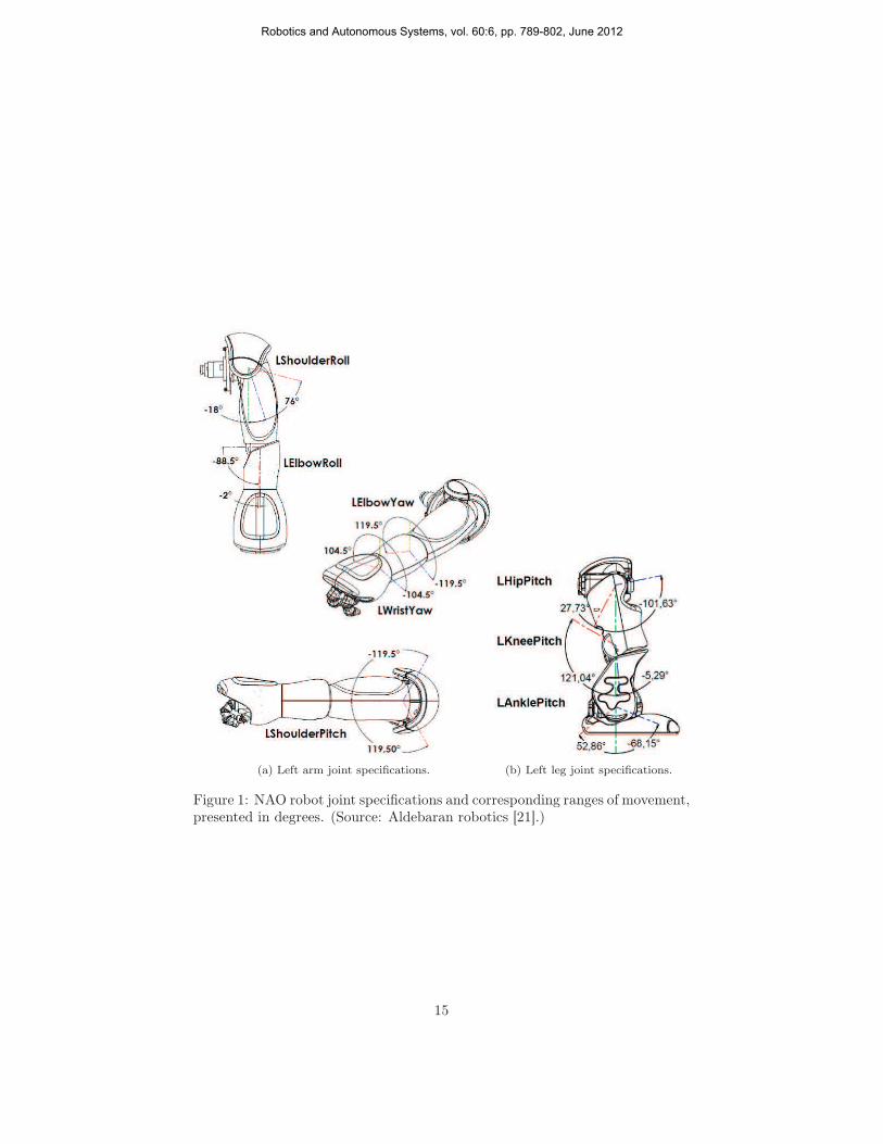
For the purposes of our experimental evaluation, we have employed the NAOrobot (academic edition), a humanoid robotic platform with 27 degrees of free-dom [21]. The training trajectories were presented to the robot by means ofkinesthetics, that is manually moving the robot’s arms and recording the jointangles. During this procedure, joint position sampling was conducted, with thesampling rate set to 20 Hz. The robot joints actively participating in each ex-periment varied according to the specification of the performed motion types(for details cf. Table 1 and Fig. 1). The aforementioned joint angle data werecollected using a fully threaded NAO-Matlab communication protocol developedby the authors in Python.

14


(a) Left arm joint specifications. (b) Left leg joint specifications.

Figure 1: NAO robot joint specifications and corresponding ranges of movement,presented in degrees. (Source: Aldebaran robotics [21].)

15


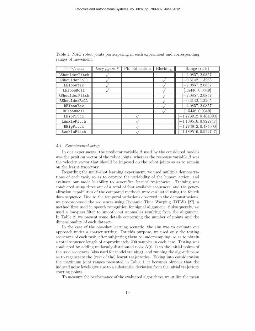
Table 1: NAO robot joints participating in each experiment and correspondingranges of movement.

Joints/Tasks Lazy figure 8 Ph. Education Blocking Range (rads)

LShoulderPitch√

[−2.0857, 2.0857]LShoulderRoll

√ √[−0.3142, 1.3265]

LElbowYaw√ √

[−2.0857, 2.0857]LElbowRoll

√ √[1.5446, 0.0349]

RShoulderPitch√

[−2.0857, 2.0857]RShoulderRoll

√[−0.3142, 1.3265]

RElbowYaw√

[−2.0857, 2.0857]RElbowRoll

√[1.5446, 0.0349]

LHipPitch√

[−1.773912, 0.484090]LAnklePitch

√[−1.189516, 0.922747]

RHipPitch√

[−1.773912, 0.484090]RAnklePitch

√[−1.189516, 0.922747]

5.1. Experimental setup

In our experiments, the predictor variable β used by the considered modelswas the position vector of the robot joints, whereas the response variable β wasthe velocity vector that should be imposed on the robot joints so as to remainon the learnt trajectory.

Regarding the multi-shot learning experiment, we used multiple demonstra-tions of each task, so as to capture the variability of the human action, andevaluate our model’s ability to generalize learned trajectories. Training wasconducted using three out of a total of four available sequences, and the gener-alization capabilities of the compared methods were evaluated using the fourthdata sequence. Due to the temporal variations observed in the demonstrations,we pre-processed the sequences using Dynamic Time Warping (DTW) [27], amethod first used in speech recognition for signal alignment. Subsequently, weused a low-pass filter to smooth out anomalies resulting from the alignment.In Table 2, we present some details concerning the number of points and thedimensionality of each dataset.

In the case of the one-shot learning scenario, the aim was to evaluate ourapproach under a sparser setting. For this purpose, we used only the testingsequences of each task, after subjecting them to undersampling, so as to obtaina total sequence length of approximately 200 samples in each case. Testing wasconducted by adding uniformly distributed noise U(0, 1) to the initial points ofthe used sequences (also used for model training), and running the algorithms soas to regenerate the (rest of the) learnt trajectories. Taking into considerationthe maximum joint ranges presented in Table 1, it becomes obvious that theinduced noise levels give rise to a substantial deviation from the initial trajectorystarting points.

To measure the performance of the evaluated algorithms, we utilize the mean

16


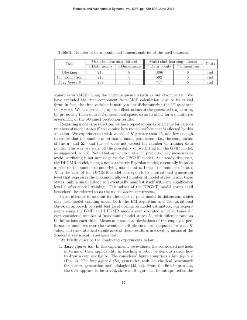
Table 2: Number of data points and dimensionalities of the used datasets.

TaskOne-shot learning dataset Multi-shot learning dataset

Units#Data points #Dimensions #Data points #Dimensions

Blocking 218 8 1086 8 radPh. Education 213 5 592 5 radLazy figure 8 239 5 717 5 rad

square error (MSE) along the entire sequence length as our error metric. Wehave excluded the time component from MSE calculation, due to its trivialform; in fact, the time variable is merely a line dichotomizing the 1st quadrant(ǫ : y = x). We also provide graphical illustrations of the generated trajectories,by projecting them onto a 2-dimensional space, so as to allow for a qualitativeassessment of the obtained prediction results.

Regarding model size selection, we have repeated our experiments for variousnumbers of model statesK to examine how model performance is affected by thisselection. We experimented with values of K greater than 25, and low enoughto ensure that the number of estimated model parameters (i.e., the componentsof the µi and Σi, and the πi) does not exceed the number of training datapoints. This way, we ward off the possibility of overfitting for the GMR model,as suggested in [20]. Note that application of such precautionary measures toavoid overfitting is not necessary for the DPGMR model. As already discussed,the DPGMR model, being a nonparametric Bayesian model, essentially imposesa prior on the number of underlying model states. Hence, the number of statesK in the case of the DPGMR model corresponds to a variational truncationlevel that expresses the maximum allowed number of model states. From thesestates, only a small subset will eventually manifest itself with any significancelevel ǫ, after model training. This subset of the DPGMR model states shallhenceforth be referred to as the model active components.

In an attempt to account for the effect of poor model initialization, whichmay lead model training under both the EM algorithm and the variationalBayesian approach to yield bad local optima as model estimators, our experi-ments using the GMR and DPGMR models were executed multiple times foreach considered number of (maximum) model states K, with different randominitializations each time. Means and standard deviations of the employed per-formance measures over the executed multiple runs are computed for each Kvalue, and the statistical significance of these results is assessed by means of theStudent-t statistical hypothesis test.

We briefly describe the conducted experiments below.

1. Lazy figure 8s: In this experiment, we evaluate the considered methodsin terms of their applicability in teaching a robot by demonstration howto draw a complex figure. The considered figure comprises a lazy figure 8(Fig. 2). The lazy figure 8 (L8) generation task is a classical benchmarkfor pattern generation methodologies [43, 44]. From the first impression,the task appears to be trivial, since an 8 figure can be interpreted as the

17


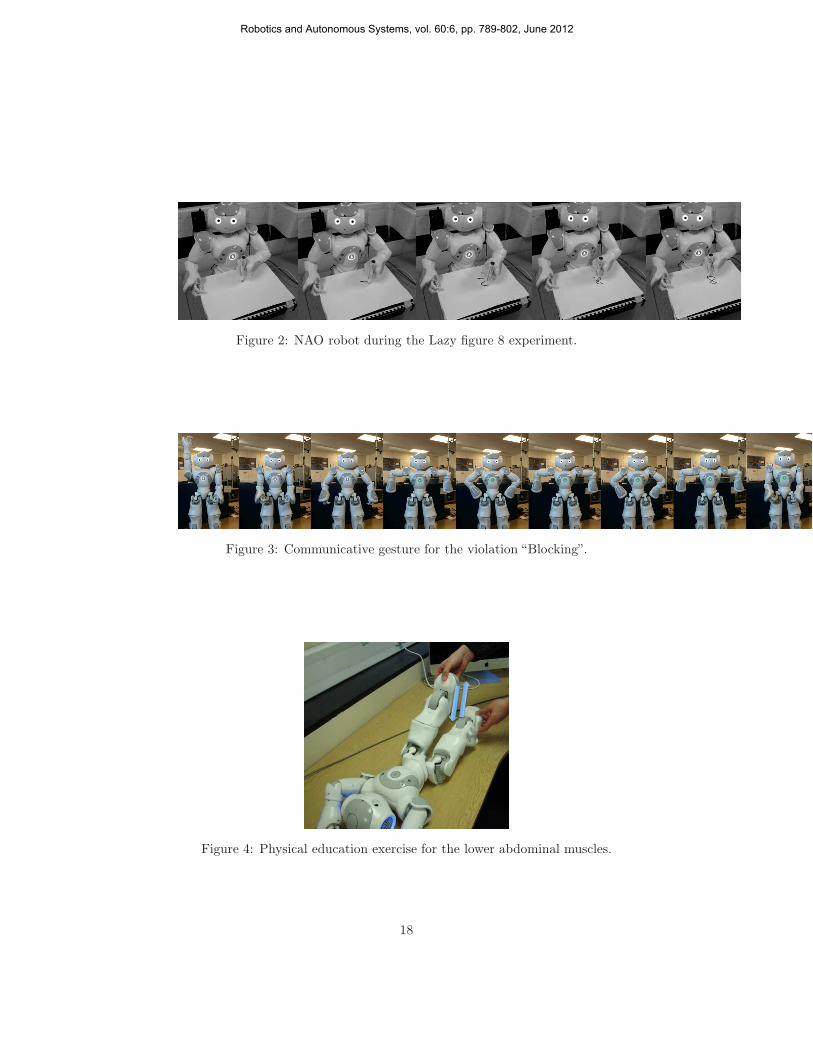
Figure 2: NAO robot during the Lazy figure 8 experiment.

Figure 3: Communicative gesture for the violation “Blocking”.

Figure 4: Physical education exercise for the lower abdominal muscles.

18


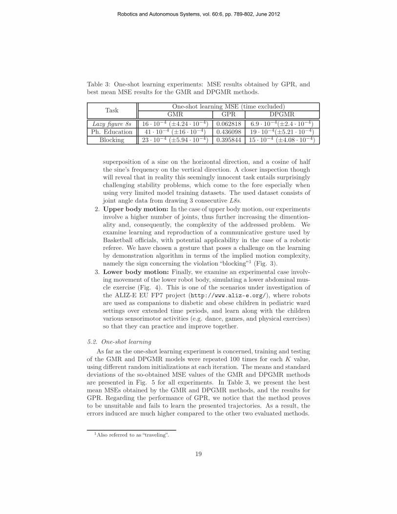
Table 3: One-shot learning experiments: MSE results obtained by GPR, andbest mean MSE results for the GMR and DPGMR methods.

TaskOne-shot learning MSE (time excluded)

GMR GPR DPGMR

Lazy figure 8s 16 · 10−4 (±4.24 · 10−4) 0.062818 6.9 · 10−4(±2.4 · 10−4)Ph. Education 41 · 10−4 (±16 · 10−4) 0.436098 19 · 10−4(±5.21 · 10−4)

Blocking 23 · 10−4 (±5.94 · 10−4) 0.395844 15 · 10−4 (±4.08 · 10−4)

superposition of a sine on the horizontal direction, and a cosine of halfthe sine’s frequency on the vertical direction. A closer inspection thoughwill reveal that in reality this seemingly innocent task entails surprisinglychallenging stability problems, which come to the fore especially whenusing very limited model training datasets. The used dataset consists ofjoint angle data from drawing 3 consecutive L8s.

2. Upper body motion: In the case of upper body motion, our experimentsinvolve a higher number of joints, thus further increasing the dimention-ality and, consequently, the complexity of the addressed problem. Weexamine learning and reproduction of a communicative gesture used byBasketball officials, with potential applicability in the case of a roboticreferee. We have chosen a gesture that poses a challenge on the learningby demonstration algorithm in terms of the implied motion complexity,namely the sign concerning the violation “blocking”1 (Fig. 3).

3. Lower body motion: Finally, we examine an experimental case involv-ing movement of the lower robot body, simulating a lower abdominal mus-cle exercise (Fig. 4). This is one of the scenarios under investigation ofthe ALIZ-E EU FP7 project (http://www.aliz-e.org/), where robotsare used as companions to diabetic and obese children in pediatric wardsettings over extended time periods, and learn along with the childrenvarious sensorimotor activities (e.g. dance, games, and physical exercises)so that they can practice and improve together.

5.2. One-shot learning

As far as the one-shot learning experiment is concerned, training and testingof the GMR and DPGMR models were repeated 100 times for each K value,using different random initializations at each iteration. The means and standarddeviations of the so-obtained MSE values of the GMR and DPGMR methodsare presented in Fig. 5 for all experiments. In Table 3, we present the bestmean MSEs obtained by the GMR and DPGMR methods, and the results forGPR. Regarding the performance of GPR, we notice that the method provesto be unsuitable and fails to learn the presented trajectories. As a result, theerrors induced are much higher compared to the other two evaluated methods.

1Also referred to as “traveling”.

19


http://www.aliz-e.org/

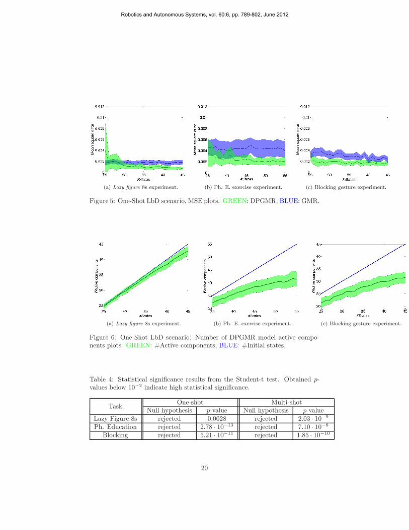
(a) Lazy figure 8s experiment. (b) Ph. E. exercise experiment. (c) Blocking gesture experiment.

Figure 5: One-Shot LbD scenario, MSE plots. GREEN: DPGMR, BLUE: GMR.


Figure 6: One-Shot LbD scenario: Number of DPGMR model active compo-nents plots. GREEN: #Active components, BLUE: #Initial states.

Table 4: Statistical significance results from the Student-t test. Obtained p-values below 10−2 indicate high statistical significance.

TaskOne-shot Multi-shot

Null hypothesis p-value Null hypothesis p-valueLazy Figure 8s rejected 0.0028 rejected 2.03 · 10−9

Ph. Education rejected 2.78 · 10−13 rejected 7.10 · 10−8

Blocking rejected 5.21 · 10−11 rejected 1.85 · 10−10

20


Regarding comparison between GMR and DPGMR, we observe that theproposed method contributes to a significantly improved performance in all theconducted experiments. The error results also are more consistent, as a muchlower standard deviation of the MSE values is achieved in almost all cases.Elaborating on that, we can see that the best DPGMR mean error is less thanhalf of that obtained by GMR in the case of the L8s experiment (≃ 43%), andthe Ph. E. exercise experiment (≃ 46%). In the blocking communicative gestureexperiment, the improvement is approximately 34%. The standard deviation ofthe observed error values is also consistently lower in most cases. The L8sexperiment was the only exception to that rule; apparently, this phenomenonoccurred as a consequence of the fact that at lower numbers of initial states(K) the truncation level of the DPGMR was obviously much less than neededto adequately model the observed trajectories, thus leading to poor model fits.Additionally, utilizing the Student-t test we are able to evaluate the statisticalsignificance of our findings, regarding the mean MSEs of GMR and DPGMRfor different numbers of states. As can be seen in Table 4, the null hypothesisthat both sequences of mean MSEs belong to distributions with the same meanis rejected with considerable certainty.

Finally, in Fig. 6 we depict the obtained mean number of DPGMR activecomponents, as well as their corresponding standard deviation. A very im-portant conclusion that can be drawn from these plots is that introduction ofa Dirichlet process prior resulted in significantly smaller models, thus avoid-ing both the unnecessary complexity and the excessive computational burdenof GMR, without the need to resort to unreliable likelihood- or entropy-basedmodel selection criteria. Indeed, the DPGMR model is able to achieve, on aver-age, up to 30% model complexity reduction compared to GMR. Note that theinferred number of active components for the DPGMR model varies dependingon the random initialization of the training algorithm, hence the obtained vari-ance of the number of active components provided in these graphs. We mustunderline though, that this variability is not an undesirable property: In thecase of the DPGMR model, the number of active components is regarded asyet another model parameter, and its value is determined in conjunction withthe values of the rest of the model parameters, so as to optimize the variationallower bound L(q) in (25). Thus, different starting points for the model trainingalgorithm will necessarily yield different local optimal for L(q), with the numberof model active components being one of the optimized parameters.

5.3. Multi-shot learning

For the multi-shot learning experiment, we have calculated the mean MSEand its standard deviation resulting from 50 repetitions of the training and test-ing procedures for the GMR and DPGMR methods, as well as the performanceof GPR. The obtained MSE results are presented in Fig. 7 for the GMR andDPGMR methods, and the best error results for the GMR and DPGMR meth-ods along with the performance of GPR are provided in Table 5. The results ofthe Student-t test regarding the comparison between GMR and DPGMR can be

21


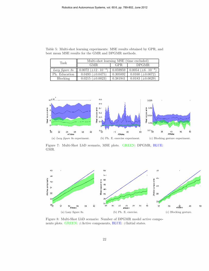
Table 5: Multi-shot learning experiments: MSE results obtained by GPR, andbest mean MSE results for the GMR and DPGMR methods.

TaskMulti-shot learning MSE (time excluded)

GMR GPR DPGMR

Lazy figure 8s 0.0072 (±12 · 10−4) 0.059959 0.0054 (±6 · 10−4)Ph. Education 0.0493 (±0.0475) 0.305892 0.0160 (±0.0072)

Blocking 0.0215 (±0.0023) 0.381941 0.0183 (±0.0029)


Figure 7: Multi-Shot LbD scenario, MSE plots. GREEN: DPGMR, BLUE:GMR.

(a) Lazy figure 8s. (b) Ph. E. exercise. (c) Blocking gesture.

Figure 8: Multi-Shot LbD scenario: Number of DPGMR model active compo-nents plots. GREEN: #Active components, BLUE: #Initial states.

22


−10 −5 0 5 10−0.6

−0.4

−0.2

0

0.2

0.4

0.6

0.8

(a) Lazy figure 8s.

−10 −5 0 5 10−1

−0.5

0

0.5

1

(b) Ph. E. exercise.

−10 −5 0 5 10 15

−1

0

1

2

(c) Blocking gesture.

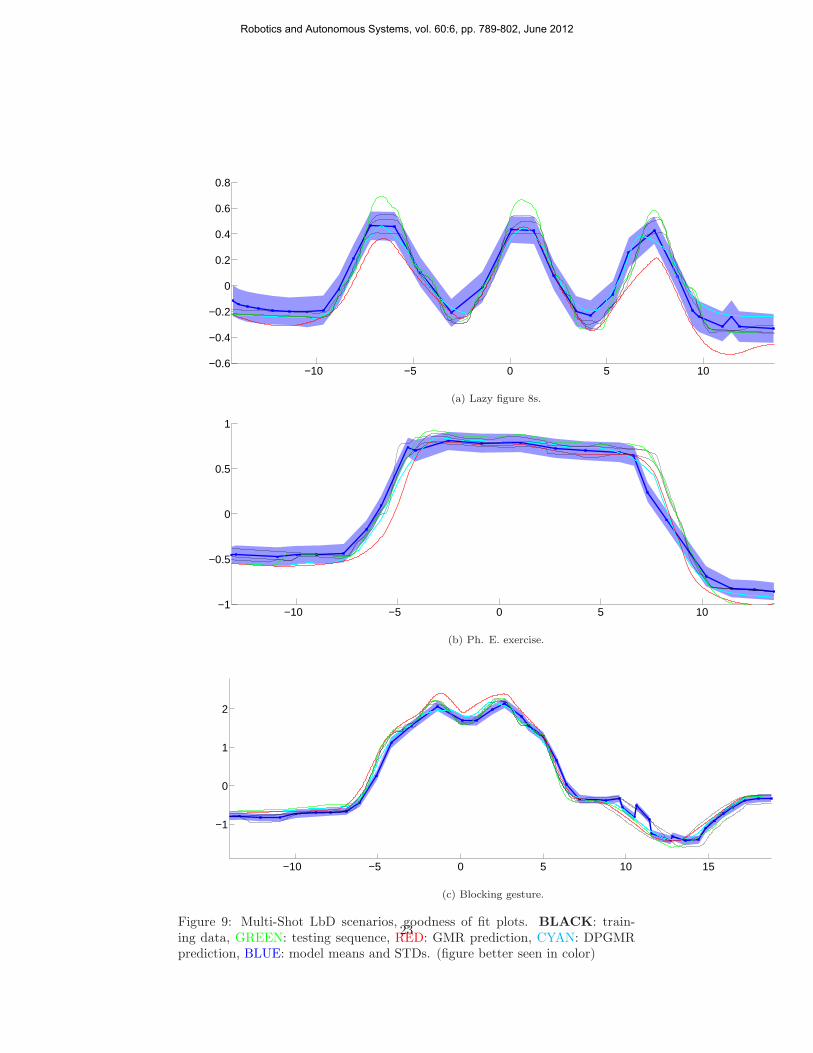
Figure 9: Multi-Shot LbD scenarios, goodness of fit plots. BLACK: train-ing data, GREEN: testing sequence, RED: GMR prediction, CYAN: DPGMRprediction, BLUE: model means and STDs. (figure better seen in color)

23


seen in Table 4, and, finally, the number of active components of the DPGMRmethod are depicted in Fig. 8.

Commenting on the results, DPGMR achieves an error reduction of approx-imately 27.7% in the L8s experiment, 66.3% in the Ph. E. experiment, and14.9% in the Blocking communicative gesture experiment, compared to GMR.The standard deviation of the DPGMR results is also lower, indicating that thepostulated model is more consistent. Even in the blocking experiment, whereTable 5 shows a higher STD for DPGMR, it can be seen in Fig. 7c that thisbehavior consists an isolated case, and the yielded STD is in general lower thanthe one obtained by GMR. The Student-t tests show an even higher statisticalsignificance of the difference between GMR and DPGMR, compared to the pre-vious experiment. Similarly, GPR does not perform adequately well and fails topredict the presented trajectories, regardless of the considerably higher numberof training data points available in this experiment.

As far as the model size is concerned, the highest reduction is achieved in thePh. E. exercise experiment, by as much as 35.9%. In the case of L8s and blockingcommunicative gesture, DPGMR yields moderately reduced models, by as muchas 6.8% and 11.4%, respectively. It should be noted that, in this experiment, thenumber of training data points vastly exceeds the number of maximum modelparameters, resulting from the selection of the maximum K values. Hence, wewould not expect the DPGMR model to yield any significant model reduction.However, our results have indicated that DPGMR obtains much smaller modelscompared to GMR even under such an experimental setting. Thus, we man-age to empirically prove the remarkable advantages of DPGMR in terms of theresulting computational efficiency, which is of crucial importance to the prac-tical applicability of learning by demonstration algorithms in modern roboticplatforms.

Concluding, in Fig. 9 we provide a graphical representation of the goodnessof fit to the data of the GMR and DPGMR models. We depict the 3 trainingsequences (in black), the testing sequence (in green), the GMR-predicted data(in red), the DPGMR-predicted data (in cyan) and the means and standard de-viations of the DPGMR model. As all trajectories are of higher dimensionalitythan can be depicted, this graph was obtained by effectively reducing the datadimensions toD = 2, by application of the Karhunen-Loeve transform (KLT). Inorder to calculate the corresponding covariance matrices of the DPGMR modelin this low-dimensional space, we obtained 1k samples from the posterior distri-butions {N (·|µm,Σm)}Mm=1, where M is the number of active components, andsubsequently found the covariance matrices of the low-dimensional projectionsof those sampled points. We observe that the DPGMR predictions fit the datamuch better than the GMR-obtained ones.

5.4. Computational Costs

Let us now investigate the computational costs of DPGMR, as compared toits considered competitors, that is GMR and GPR. As one may expect, basedon Eqs. (29)-(45), DPGMR training for a given value of the maximum numberof model states K requires exactly the same computational costs as GMR for

24


the same value of K. Additionally, as already discussed, GMR also demandstraining multiple models (for different K values) to select from, which is notthe case for the DPGMR, which conducts inference over the proper number ofmodel states. As such, DPGMR training eventually turns out to be much moreefficient than GMR training, as the need of training multiple models to selectfrom gets obviated in the case of DPGMR.

Regarding, real-time testing, we have observed that DPGMR offers a con-siderable improvement in the required computational times over GMR, which,not surprisingly, is almost equal to the model size reduction it offers comparedto GMR. This was expectable enough, given the expression of the DPGMR-generated predictions (61), which shows that a GMR and a DPGMR modelwith the same number of states impose exactly the same computational coststo generate predictions, which increase in a linear fashion with the effective sizeof the models.

Finally, we would like to mention that both GMR and DPGMR are consider-ably more efficient compared to GPR. Indeed, contrary to GMR and DPGMR,GPR costs increase with the number of model training data points. As such, itcame to no surprise to us that GPR required 2 orders of magnitude longer timeto generate a prediction, compared to GMR and DPGMR, in the case of themulti-shot scenario, and double the time in the case of the one-shot scenario. Inany case, we would like to mention that the longest GMR and DPGMR requiredto generate a prediction was of the order of 10−3 seconds, a figure which got ashigh as 0.3 seconds in the case of GPR.

6. Conclusions

In this paper, we presented a nonparametric Bayesian approach towardstrajectory-based robot learning by demonstration. The proposed approach isbased on the postulation of a Gaussian mixture regression model comprisinga countably infinite number of states, and is facilitated by the imposition of aDirichlet process prior over the model states. The proposed approach allowsfor the automatic determination of the proper number of GMR model states,without the need of resorting to model order selection criteria, application ofwhich is rather tedious and notorious for yielding noisy model order estimateswith heavy overfitting proneness.

Our novel approach was evaluated considering a number of experimental sce-narios, and its performance was compared to state-of-the-art robot learning bydemonstration methodologies based on Gaussian mixture regression and Gaus-sian process regression. As we showed, our method, exploiting the robustnessof Bayesian estimation, and the effectiveness of nonparametric Bayesian modelsin automatic model size determination, allows for a significant performance in-crease, while imposing computational requirements for trajectory regenerationsimilar to the GPR/GMR methods, since prediction under all these approacheseventually reduces to a sum of linear regression models. The MATLAB imple-mentation of the DPGMR method shall be made available through the websitesof the authors.

25


Acknowledgment

This work has been partially funded by the EU FP7 ALIZ-E project (grant248116).

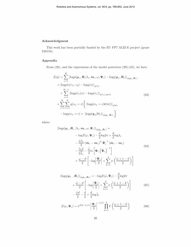
Appendix

From (28), and the expressions of the model posteriors (29)-(45), we have

L(q) =K∑

c=1

〈logp(µc,Rc|λc,mc, ω,Ψc)− logq(µc,Rc)〉q(µc,Rc)

+ 〈logp(α|γ1, γ2)− logq(α)〉q(α)

+

K−1∑

c=1

〈logp(vc|α)− logq(vc)〉q(vc),q(α)

+

K∑

c=1

N∑

n=1

q(xn = c)

{〈logp(xn = c|π(v))〉q(v)

− logq(xn = c) + 〈logp(yn|Θc)〉q(µc,Rc)

}

(63)

where

〈logp(µc,Rc |λc,mc, ω,Ψc)〉q(µc,Rc)

=

− logZ(ω,Ψc)−d

2log2π +

d

2logλc

− ωλc2

(mc −mc)TΨ

−1

c (mc −mc)

− λcd

2λc− ω

2tr

[Ψc

(Ψc

)−1]

+ω − d

2

[−log

∣∣∣∣Ψc

2

∣∣∣∣+d∑

k=1

ψ

(ω + 1− k

2

)]

(64)

〈logq(µc ,Rc)〉q(µc,Rc)

= −logZ(ω, Ψc)−d

2log2π

+ω − d

2

[−log

∣∣∣∣Ψc

2

∣∣∣∣+d∑

k=1

ψ

(ω + 1− k

2

)]

− ωd

2− d

2+d

2logλc

(65)

Z(ω,Ψc) = πd(d−1)/4

∣∣∣∣Ψc

2

∣∣∣∣−ω/2 d∏

k=1

Γ

(ω + 1− k

2

)(66)

26


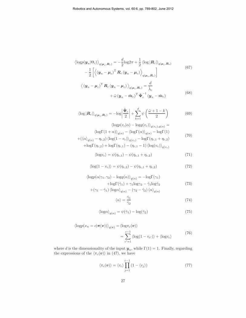
⟨logp(yn|Θc)

⟩q(µ

c,Rc)

= −d2log2π +

1

2〈log |Rc|〉q(µ

c,Rc)

− 1

2

[⟨(yn − µc)

TRc (yn − µc)

⟩q(µ

c,Rc)

] (67)

⟨(yn − µc)

TRc (yn − µc)

⟩q(µ

c,Rc)

=d

λc

+ ω (yn − mc)TΨ

−1

c (yn − mc)(68)

〈log |Rc|〉q(µc,Rc)

= −log

∣∣∣∣Ψc

2

∣∣∣∣+d∑

k=1

ψ

(ω + 1− k

2

)(69)

〈logp(vc|α)− logq(vc)〉q(vc),q(α) =〈logΓ(1 + α)〉q(α) − 〈logΓ(α)〉q(α) − logΓ(1)

+(〈α〉q(α) − ηc,2) 〈log(1− vc)〉q(vc) − logΓ(ηc,1 + ηc,2)

+logΓ(ηc,2) + logΓ(ηc,1)− (ηc,1 − 1) 〈log(vc)〉q(vc)

(70)

〈logvc〉 = ψ(ηc,1)− ψ(ηc,1 + ηc,2) (71)

〈log(1 − vc)〉 = ψ(ηc,2)− ψ(ηc,1 + ηc,2) (72)

〈logp(α|γ1, γ2)− logq(α)〉q(α) = −logΓ(γ1)

+logΓ(γ1) + γ1logγ2 − γ1logγ2

+(γ1 − γ1) 〈logα〉q(α) − (γ2 − γ2) 〈α〉q(α)(73)

〈α〉 = γ1γ2

(74)

〈logα〉q(α) = ψ(γ1)− log(γ2) (75)

〈logp(xn = c|π(v))〉q(v) = 〈logπc(v)〉

=

c−1∑

c′=1

〈log(1− vc′)〉+ 〈logvc〉(76)

where d is the dimensionality of the input yn, while Γ(1) = 1. Finally, regardingthe expressions of the 〈πc(v)〉 in (47), we have

〈πc(v)〉 = 〈vc〉c−1∏

j=1

(1− 〈vj〉) (77)

27


where〈vc〉 =

ηc,1ηc,1 + ηc,2

(78)

In the above, ψ(.) denotes the Digamma function, and Γ(·) the Gamma function.

[1] A. Billard, S. Calinon, R. Dillmann, and S. Schaal, “Robot pro-gramming by demonstration,” in Handbook of Robotics, B. Sicilianoand O. Khatib, Eds., Secaucus, NJ, USA: Springer-Verlag, 2008,pp. 1371–1394.

[2] B. Argall, S. Chernova, M. Veloso, and B. Browning, “A surveyof robot learning from demonstration,” Robotics and AutonomousSystems, 57 (2009) 469–483.

[3] A. Skoglund, B. Iliev, and R. Palm, “Programming-by-demonstration of reaching motions–a next-state-planner ap-proach,” Robotics and Autonomous Systems, 58 (2010) 607 – 621.

[4] A. Billard, Y. Epars, S. Calinon, S. Schaal, and G. Cheng, “Dis-covering optimal imitation strategies,” Robotics and AutonomousSystems, 47 (2004) 69 – 77.

[5] A. Billard and M. J. Mataric, “Learning human arm movementsby imitation:: Evaluation of a biologically inspired connectionistarchitecture,” Robotics and Autonomous Systems, 37 (2001) 145 –160.

[6] M. Lopes and J. Santos-Victor, “A developmental roadmap forlearning by imitation in robots,” IEEE Transactions in SystemsMan and Cybernetic - Part B: Cybernetics 37 (2007) 308 - 321.

[7] P. Pastor, H. Hoffmann, T. Asfour, and S. Schaal, “Learning andgeneralization of motor skills by learning from demonstration,” inRobotics and Automation, 2009. ICRA ’09. IEEE InternationalConference on Robotics and Automation, May 2009, pp. 763 –768.

[8] M. Lopes and J. Santos-Victor, “Visual learning by imitation withmotor representations,” IEEE Transactions on Systems, Man andCybernetics - Part B: Cybernetics, 35 (2005) 438–449.

[9] K. Yamane and Y. Nakamura, “Dynamics filter-concept and im-plementation of online motion generator for human figures,” IEEETrans. Robot. Autom., 19 (2003) 421–432.

[10] B. D. Argall, S. Chernova, M. Veloso, and B. Browning, “A surveyof robot learning from demonstration,” Robotics and AutonomousSystems, 57 (2009) 469–483.

[11] S. Vijayakumar, A. D’Souza, T. Shibata, J. Conradt, and S. Schaal,“Statistical learning for humanoid robots,” Autonomous Robots, 12(2002) 55–69.

28


[12] S. Vijayakumar, M. Toussaint, G. Petkos, M. Howard, B. Send-hoff, E. Korner, O. Sporns, H. Ritter, and K. Doya, “Planningand moving in dynamic environments: A statistical machine learn-ing approach.”, in (eds.) Sendhoff, Koerner, Sporns, Ritter, Doya,Creating Brain Like Intelligence: From Principles to Complex In-telligent Systems, LNAI-Vol. 5436, Springer-Verlag, 2009.

[13] K. M. Chai, S. Klanke, C. Williams, and S. Vijayakumar, “Multi-task gaussian process learning of robot inverse dynamics,” in Proc.Advances in Neural Information Processing Systems (NIPS ’08),Vancouver, Canada, 2008.

[14] S. Vijayakumar, A. D’Souza, and S. Schaal, “Incremental onlinelearning in high dimensions,” Neural Computation, 17 (2005) 2602–2634.

[15] Z. Ghahramani and M. I. Jordan, “Supervised learning from in-complete data via an EM approach,” in Advances in Neural Infor-mation Processing Systems, 6, 1994, pp. 120–127.

[16] A. G. Billard, S. Calinon, and F. Guenter, “Discriminative andadaptive imitation in uni-manual and bi-manual tasks,” Roboticsand Autonomous Systems, 54 (2006) 370 – 384.

[17] A. Dempster, N. Laird, and D. Rubin, “Maximum likelihood fromincomplete data via the EM algorithm,” Journal of the Royal Sta-tistical Society, B, 39 (1977) 1–38.

[18] D. Lee and Y. Nakamura, “Mimesis scheme using a monocular vi-sion system on a humanoid robot,” in Proc. IEEE InternationalConference on Robotics and Automation (ICRA), 2007, pp. 2162–2168.

[19] G. Schwarz, “Estimating the dimension of a model,” The Annalsof Statistics, 4 (1978) 461–464.

[20] G. McLachlan and D. Peel, Finite Mixture Models. Wiley Seriesin Probability and Statistics, 2000.

[21] Aldebaran robotics, ”NAO robot academic edition”, http://www.aldebaran-robotics.com/.

[22] S. Chatzis, D. Kosmopoulos, and T. Varvarigou, “Signal modelingand classification using a robust latent space model based on tdistributions,” IEEE Trans. Signal Processing, 56 (2008) 949–963.

[23] S. Walker, P. Damien, P. Laud, and A. Smith, “Bayesian nonpara-metric inference for random distributions and related functions,”J. Roy. Statist. Soc. B, 61 (1999) 485–527.

29


http://www.aldebaran-robotics.com/

http://www.aldebaran-robotics.com/

[24] R. Neal, “Markov chain sampling methods for Dirichlet processmixture models,” J. Comput. Graph. Statist., 9 (2000) 249–265.

[25] P. Muller and F. Quintana, “Nonparametric Bayesian data analy-sis,” Statist. Sci., 19 (2004) pp. 95–110.

[26] C. Antoniak, “Mixtures of Dirichlet processes with applicationsto Bayesian nonparametric problems.” The Annals of Statistics,2 (1974) 1152–1174.

[27] C. S. Myersand and L. R. Rabiner, “Acomparativestudyofseveraldynamic time-warping algorithms for connected word recognition.”The Bell System Technical Journal, vol. 60, no. 7, pp. 1389–1409,September 1981.

[28] J. Sethuraman, “A constructive definition of the Dirichlet prior,”Statistica Sinica, 2 (1994) 639–650.

[29] D. Blei and M. Jordan, “Variational methods for the Dirichlet pro-cess,” in 21st Int. Conf. Machine Learning, New York, NY, USA,July 2004, pp. 12–19.

[30] C. M. Bishop, Pattern Recognition and Machine Learning. NewYork: Springer, 2006.

[31] V. N. Vapnik, Statistical Learning Theory. New York: Wiley,1998.

[32] C. E. Rasmussen and C. K. I. Williams, Gaussian Processes forMachine Learning. MIT Press, 2006.

[33] B. G. Leroux, “Consistent estimation of a mixing distribution,”Annals of Statistics, 20 (1992) 1350–1360.

[34] G. Celeux and G. Soromenho, “An entropy criterion for assessingthe number of clusters in a mixture model,” Classification Journal,13 (1996) 195–212.

[35] T. Ferguson, “A Bayesian analysis of some nonparametric prob-lems,” The Annals of Statistics, 1 (1973) 209–230.

[36] D. Blackwell and J. MacQueen, “Ferguson distributions via Pólyaurn schemes,” The Annals of Statistics, 1 (1973) 353–355.

[37] D. M. Blei and M. I. Jordan, “Variational inference for Dirichletprocess mixtures,” Bayesian Analysis, 1 (2006) 121–144.

[38] Y. Qi, J. W. Paisley, and L. Carin, “Music analysis using hiddenMarkov mixture models,” IEEE Transactions on Signal Processing,55 (2007) 5209–5224.

30


[39] M. Jordan, Z. Ghahramani, T. Jaakkola, and L. Saul, “An intro-duction to variational methods for graphical models,” in Learningin Graphical Models, M. Jordan, Ed. Dordrecht: Kluwer, 1998,pp. 105–162.

[40] D. Chandler, Introduction to Modern Statistical Mechanics. NewYork: Oxford University Press, 1987.

[41] D. Grimes, R. Chalodhorn, and R. Rao, “Dynamic imitation in ahumanoid robot through nonparametric probabilistic inference.” inProc. Robotics: Science and Systems (RSS), 2006, pp. 1–8.

[42] D. Nguyen-Tuong and J. Peters, “Local gaussian process regressionfor real-time model-based robot control,” in IEEE/RSJ Int. Conf.on Intelligent Robots and Systems (IROS), 2008, pp. 380–385.

[43] B. Pearlmutter, “Gradient calculation for dynamic recurrent neuralnetworks: A survey,” IEEE Transactions on Neural Networks, 6(1995) 1212–1228.

[44] P. Zegers and M. K. Sundareshan, “Trajectory generation and mod-ulation using dynamic neural networks,” IEEE Transactions onNeural Networks 14 (2003) 520–533.

[45] Y. Demiris and B. Khadhouri, “Hierarchical attentive multiplemodels for execution and recognition (HAMMER),” Robotics andAutonomous Systems, 54 (2006) 361–369.

[46] R. Ros, I. Baroni, M. Nalin, and Y. Demiris, "Adapting robotbehavior to user’s capabilities: a dance instruction study," in Proc.6th international conference on Human-robot interaction, 2011, pp.235–236.

31


Documents

A Nonparametric Bayesian Approach Towards Robot Learning by … · 2014-06-01 · A Nonparametric Bayesian Approach Towards Robot Learning by Demonstration Sotirios P. Chatzis, Dimitrios