A Note on Capital Budgeting in the Purchase of Information

ABRAHAM MEHREZ and ALAN STULMAN Department of Industrial Engineering and Management, Ben-Gurion University of the Negev, Beer Sheva, Israel

A capital budgeting problem of purchasing perfect information is defined. The relationship between this problem and the Expected Value measure is shown and an illustrative example provided.

INTRODUCTION

A company, when deciding about its participation in some proposed project, generally must make the decision under conditions of uncertainty about the outcome of the project. The firm should engage in research about the proposed project if the cost of the research is compensated for by an improved expected present worth of the project. Research will be defined as any activity such as marketing, R & D, etc., which spends money to reduce the uncer- tainties of the project.

Ideally, research should eliminate all of the un- certainty about the project before the compnay must make its decision. In reality, this is often impossible or else prohibitively expensive. Instead, a company will use its limited research funds to purchase partial information, that is, to reduce un- certainty but not necessarily eliminate it.

Here we will consider two types of companies - a neutral-risk company and a risk-averse company - faced with a portfolio of such projects. We will assume that for each project in the portfolio the company can institute research and eliminate all of the uncertainty. The research required for all the projects will perhaps be too expensive and thus we will assume a budgetary constraint. Also we will assume that the situation of each project does not allow for the purchase of partial information. The company will either do not research on the project or will spend the required sum to do complete research. An example of such a project may be where the research is paying another company not to enter a market in order to ensure its own posi- tion in the market.

Let us assume that the expected value of all the projects in the portfolio are increased by the com- pany’s decision as to which projects to research. Later, when the company is faced with the capital budgeting decisions about which project actually to carry out, their choice will be a better one. They will be choosing from a portfolio with better ex-

pected returns than the pre-researched portfolio. In the next section we formulate the problem assum- ing that the compnay is risk-neutral. In the third Section we will observe the decisions of a risk- averse company by means of an illustrative example.

THE MODEL FOR THE RISK-NEUTRAL COMPANY

Let Xi be a random variable representing the dis- counted present value of project i in the portfolio of n projects. A company will choose the project unresearched only if E(Xi) is positive. Then the value of having the project in the company’s port- folio is given by max{E(Xi), 0). This expression, called the ‘Recourse Problem’, was defined by Walkup and Wets (1967). If the company decides on researching the project, it will then only choose the project if Xi is positive. Thus, the expected value for having the project in the company’s port- folio, given that it will be researched, is given by E{Max (y, 0)). This term can be found in the liter- ature and is called the ‘Wait and See Problem’, discussed by Madansky (1960). The difference be- tween the two is called the Expected Value of Perfect Information (EVPI (Xi)) and is the most that the company should be willing to pay for information about project i. The EVPI has been discussed by many authors in the literature, includ- ing Gunderson and Morris (1978), Huang et al. (1977), Ben-Tal and Hochman (1972) and Avriel and Williams (1977). Recently some aspects of the distributional properties of the EVPI were studied by Mehrez and Stulman (1982) with respect to the project-selection problem.

Let us define q to be an indicator variable, equal to one if research into project i is undertaken, and zero otherwise. Let vi = 1 - q. Then the total ex- pected present value of all the projects in the

0 Wiley Heyden Ltd, 1984

CCC-0143-6570/84/ooO5-0251$02.00

MANAGERIAL AND DECISION ECONOMICS, VOL. 5, NO. 4, 1984 251

portfolio is given by

Z = uiE(max{Xi,O})+ 2 vi max{E(&),O} (1)

If ci is the cost of researching project i, and co is budget constraint, then our problem becomes

max Z

i = l i = l

s.t. 4 + z l i = 1 , y = o , 1 i : 4 c i s c , (2) i = l

Now we can write Eqn (1) as

Z = yE(max{X,,O})+ (i-u,)max{E(X,),O}

(3) i = l r = l

or n "

z = C y EVPI(X,)+ C m a x { ~ ( x , ) , 01 (4)

Since the second term in this last expression does not involve 4 in any way, then we need not con- sider it when choosing the y to maximize Z, sub- ject to the constraints in Eqn (2). Thus our problem reduces to

i = l i = l

"

s.t. y =o, 1 2 u,ci s cg i = l

The meaning of this is that a company will max- imize the total value of their portfolio subject to the budgetary constraint if they choose those projects that give them the largest total expected value of perfect information. Note that Eqn (5) is just a knapsack problem, easily solvable by the standard methods of integer programming.

An Example

Let us consider the following problem. The port- folio of the firm is given by four projects, each with a different symmetric distribution Xi, having a zero mean, equal variance u: = uz and equal costs ci =

cl. The data of these projects are given in Table 1. Thus Eqn ( 5 ) is reduced to

4

m a x Z = u C y~~ i = l A

s.t. C qscoic , y =o, 1 i = l

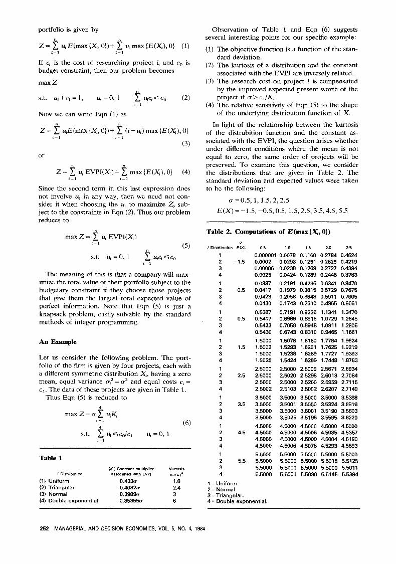
Table 1 ( K , ) Constant multiplier Kurtosis

i Distribution associated with WPI rrdrrs' (1) Uniform 0.4330 1.8 (2) Triangular 0.40820 2.4 (3) Normal 0.39890 3 (4) Double exponential 0.353550 6

Observation of Table 1 and Eqn (6) suggests several interesting points for our specific example:

(1) The objective function is a function of the stan- dard deviation.

(2) The kurtosis of a distribution and the constant associated with the EVPI are inversely related.

(3) The research cost on project i is compensated by the improved expected present worth of the project if (T > cl/Ki.

(4) The relative sensitivity of Eqn ( 5 ) to the shape of the underlying distribution function of X.

In light of the relationship between the kurtosis of the distrubition function and the constant as- sociated with the EVPI, the question arises whether under different conditions where the mean is not equal to zero, the same order of projects will be preserved. To examine this question, we consider the distributions that are given in Table 2. The standard deviation and expected values were taken to be the following:

u=0.5,1,1.5,2,2.5 E(X)=-1.5, -0.5,0.5,1.5,2.5,3.5,4.5,5.5

Table 2. Computations of E(max {Xt, 0)) (I

i Distribution E(X) 0.5 1 .o 1.5 2.0 2.5

1 0.000001 0.0078 0.1160 0.2784 0.4624 2 -1.5 0.0002 0.0293 0.1251 0.2625 0.4219 3 0.00006 0.0238 0.1269 0.2727 0.4394 4 0.0025 0.0424 0.1289 0.2448 0.3783

1 0.0387 0.2191 0.4236 0.6341 0.8470

3 0.0423 0.2058 0.3948 0.5911 0.7905 4 0.0430 0.1743 0.3310 0.4965 0.6661

1 0.5387 0.7191 0.9236 1.1341 1.3470 2 0.5 0.5417 0.6969 0.8815 1.0729 1.2645 3 0.5423 0.7058 0.8948 1.0911 1.2905 4 0.5430 0.6743 0.8310 0.9465 1.1661

1 1.5000 1.5078 1.6160 1.7784 1.9624 2 1.5 1.5002 1.5293 1.6251 1.7625 1.9219 3 1.5000 1.5238 1.6269 1.7727 1.9393 4 1.5025 1.5424 1.6289 1.7448 1.8783

1 2.5000 2.5000 2.5009 2.5671 2.6934 2 2.5 2.5000 2.5020 2.5298 2.6013 2.7084 3 2.5000 2.5000 2.5200 2.5959 2.71 15 4 2.5002 2.5103 2.5002 2.6207 2.7149

1 3.5000 3.5000 3.5000 3.5000 3.5398 2 3.5 3.5000 3.5001 3.5050 3.5324 3.5918 3 3.5000 3.5000 3.5001 3.5190 3.5803 4 3.5000 3.5025 3.5196 3.5595 3.6220 1 4.5000 4.5000 4.5000 4.5000 4.5000 2 4.5 4.5000 4.5000 4.5006 4.5085 4.5357 3 4.5000 4.5000 4.5000 4.5004 4.5190 4 4.5000 4.5006 4.5076 4.5293 4.5693

1 5.5000 5.5000 5.5000 5.5000 5.5000 2 5.5 5.5000 5.5000 5.5000 5.5018 5.5125 3 5.5000 5.5000 5.5000 5.5000 5.501 1 4 5.5000 5.5001 5.5030 5.5145 5.5394

2 -0.5 0.0417 0.1979 0.3815 0.5729 0.7675

1 =Uniform. 2 = Normal. 3 =Triangular. 4 = Double exponential.

252 MANAGERIAL AND DECISION ECONOMICS, VOL. 5, NO. 4, 1984

Clearly, the optimal order of project selection de- pends on E(max(X,,O}). In Table 2 these values are computed to the fourth decimal point.

The following computations can be verified from the results of Table 2. The optimal selection of the projects that was found for the case where E(X) = 0 holds as long as a > \ E ( X ) \ . This order is in- versely related to the kurtosis. Where (T < IE(X)l, the order is reversed. Thus, it is demonstrated that the relationship between the kurtosis and the EVPI is not clear-cut.

In addition, we observe that for a given standard deviation, the overall value of the project increases as the absolute value of the expected value of the project increases. This result has been verified in a more general structure by Mehrez and Stulman (1982). Finally, we observe that the overall value of

the project increases as the standard deviation in- creases.

A MODEL FOR A RISK-AVERSE COMPANY

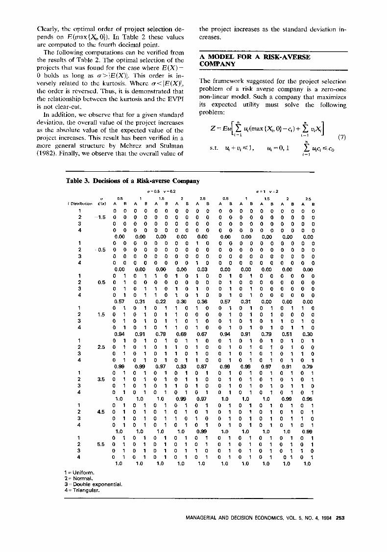
The framework suggested for the project selection problem of a risk averse company is a zero-one non-linear model. Such a company that maximizes its expected utility must solve the following problem:

Table 3. Decisions of a Risk-averse Company 0=0.5 v=0.2 o = l v = 2

u 0.5 1 1.5 2 2.5 0.5 1 1.5 2 2.5 iDistribution E ( x ) A B A B A B A B A B A B A B A B A B A B

1 2 3 4

1 2 3 4

1 2 3 4

1 2 3 4

1 2 3 4

1 2 3 4

1 2 3 4

1 2 3 4

-1.5

-0.5

0.5

1.5

2.5

3.5

4.5

5.5

0 0 0 0 0 0 0 0 0.00 0 0 0 0 0 0 0 0 0.00 0 1 0 1 0 1 0 1 0.57 0 1 0 1 0 1 0 1 0.94 0 1 0 1 0 1 0 1 0.99 0 1 0 1 0 1 0 1 1 .o 0 1 0 1 0 1 0 1 1 .o 0 1 0 1 0 1 0 1 1 .o

1 = Uniform. 2 = Normal. 3 = Double exponential. 4= Triangular.

0 0 0 0 0 0 0 0 0.00 0 0 0 0 0 0 0 0 0.00 0 1 0 0 0 1 0 1 0.31 0 1 0 1 0 1 0 1 0.91 0 1 0 1 0 1 0 1 0.99 0 1 0 1 0 1 0 1 1 .o 0 1 0 1 0 1 0 1 1 .o 0 1 0 1 0 1 0 1 1 .o

0 0 0 0 0 0 0 0 0.00 0 0 0 0 0 0 0 0 0.00 1 0 0 0 1 0 1 0 0.22 0 1 0 1 0 1 0 1 0.79 0 1 0 1 0 1 0 1 0.97 0 1 0 1 0 1 0 1 1 .o 0 1 0 1 0 1 0 1 1 .o 0 1 0 1 0 1 0 1 1 .o

0 0 0 0 0 0 0 0 0.00 0 0 0 0 0 0 0 0 0.00 1 0 0 0 1 0 1 0 0.30 1 0 1 0 1 0 1 0 0.69 0 1 1 0 1 0 0 1 0.93 0 1 0 1 1 0 0 1 0.99 0 1 0 1 1 0 0 1 1 .o 0 1 0 1 0 1 0 1 1 .o

0 0 0 0 0 0 0 0 0.00 1 0 0 0 0 0 1 0 0.03 1 0 0 0 1 0 1 0 0.36 1 0 0 0 1 0 1 0 0.67 1 0 1 0 1 0 1 0 0.87 0 1 1 0 1 0 0 1 0.97 0 1 0 1 1 0 0 1 0.99 0 1 0 1 1 0 0 1 1 .o

0 0 0 0 0 0 0 0 0.00

0 0 0 0 0 0 0 0 0.00 0 1 0 1 0 1 0 1 0.57 0 1 0 1 0 1 0 1 0.94 0 1 0 1 0 1 0 1 0.99 0 1 0 1 0 1 0 1 1 .o 0 1 0 1 0 1 0 1 1 .o

0 1 0 1 0 1 0 1

1 .o

0 0 0 0 0 0 0 0 0.00 0 0 0 0 0 0 0 0 0.00 0 1 0 0 0 1 0 1 0.31 0 1 0 1 0 1 0 1 0.91 0 1 0 1 0 1 0 1 0.99 0 1 0 1 0 1 0 1 1 .o 0 1 0 1 0 1 0 1 1 .o 0 1 0 1 0 1 0 1 1 .o

0 0 0 0 0 0 0 0 0.00 0 0 0 0 0 0 0 0 0.00 0 0 0 0 0 0 0 0 0.00 0 1 0 1 0 1 0 1 0.79 0 1 0 1 0 1 0 1 0.97 0 1 0 1 0 1 0 1 1 .o

0 1 0 1 0 1 0 1 1 .o 0 1 0 1 0 1 0 1 1 .o

0 0 0 0 0 0 0 0 0.00 0 0 0 0 0 0 0 0 0.00 0 0 0 0 0 0 0 0 0.00 0 1 0 0 1 0 0 1 0.51 0 1 0 1 0 1 0 1 0.91 0 1 0 1 0 1 0 1 0.99 0 1 0 1 0 1 0 1 1 .o 0 1 0 1 0 1 0 1 1 .o

0 0 0 0 0 0 0 0 0.00 0 0 0 0 0 0 0 0 0.00 0 0 0 0 0 0 0 0 0.00 1 0 0 0 1 0 1 0 0.30 0 1 0 0 1 0 0 1 0.79 0 1 0 1 1 0 0 1 0.95 0 1 0 1 1 0 0 1 0.99 0 1 0 1 1 0 0 1 1 .o

MANAGERIAL AND DECISION ECONOMICS, VOL. 5, NO. 4, 1984 253

where all the parameters of Eqn (7) were defined in Eqns (1) and (2). There are different methods of solving Eqn (7). For illustrative purposes, we enum- erate the solution of Eqn (7) for specific examples in Table 3. The utility function that was chosen satisfies the property of constant risk-aversion. The function is of the form u = 1 -e-*'", where l l v is a constant that determines the degree of risk- aversion.

In Table 3, we define two columns, A and B. Column A refers to the decision to purchase infor- mation. Column B refers to the decision to accept or reject the project without purchasing informa- tion. The value l denotes a decision to purchase information or to accept the project. The value 0 denotes the decision not to purchase information or to reject the project. From Table 3 we observe that when E ( X ) ? a (D =0S, 1, lS), we accept all the projects without purchasing information. The rank of the projects is

(1) Uniform (2) Triangular (3) Double exponential (4) Normal

For large expected values and large standard deviations (u = 2,2.5) we will purchase information

in the following order:

(1) Double exponential (2) Triangular (3) Uniform (4) Normal

Clearly, the less expensive is the cost of informa- tion, the more it is worthwhile to purchase it.

Finally, we observe that for a given expected value, the larger the standard deviation, the smaller is the value of the project.

CONCLUSION

This paper discusses an important problem of pur- chasing perfect information. We do agree that the analysis which was provided suffers from some limi- tations. First, it deals only with perfect information and not with more realistic structures of imperfect information. Second, it illustrates by examples and the results are not generalized. However, the data that are reported in this paper show that the solu- tion is very sensitive to the statistical parameters, and it is shown that each problem has its own characteristics and solution properties.

REFERENCES

N. Avriel and A. C. Williams (1970). The value of information and stochastic programming. Ops. Res. 18, 947-54.

A. Ben-Tal. and E. Hochman (1972). More bounds on the expectation of a convex function of a random variable. J. Appl. Prob. 9, 803-12.

H. S. Gunderson and J. G. Morris (1978). Stochastic pro- gramming with resource: a modification from an applica- tion viewpoint. J. Opl. Res. Soc. 29, 8, 769-78.

C. C. Huang, 1. Vertinsky and W. T. Ziemba (1977). Sharp

bounds on the value of perfect information. Ops. Res. 25, 1, 128-39.

A. Madansky (1960). Inequalities for stochastic linear pro- gramming problems. Mgmt. Sci. 6, 197-204.

A. Mehrez and A. Stulman (1982). Some aspects of the distributional properties of the expected value of perfect information (EVPI). J. Opl. Res. SOC. 33, 827-36.

D. W. Walkup and R. J.-B. Wets (1967). Stochastic program- ming with resource, SIAM, J. Appl. Math. 15, 1299-1314.

254 MANAGERIAL AND DECISION ECONOMICS, VOL. 5, NO. 4, 1984