A note on Jones polynomial and cosmetic surgery

“3-Wu” — 2019/10/30 — 23:55 — page 1087 — #1

Communications inAnalysis and GeometryVolume 27, Number 5, 1087–1104, 2019

A note on Jones polynomial and

cosmetic surgery

Kazuhiro Ichihara and Zhongtao Wu

We show that two Dehn surgeries on a knot K never yield mani-folds that are homeomorphic as oriented manifolds if V ′′

K(1) 6= 0 orV ′′′K (1) 6= 0. As an application, we verify the cosmetic surgery con-

jecture for all knots with no more than 11 crossings except for three10-crossing knots and five 11-crossing knots. We also compute thefinite type invariant of order 3 for two-bridge knots and Whiteheaddoubles, from which we prove several nonexistence results of purelycosmetic surgery.

1. Introduction

Dehn surgery is an operation to modify a three-manifold by drilling andthen regluing a solid torus. Denote by Yr(K) the resulting three-manifoldvia Dehn surgery on a knot K in a closed orientable three-manifold Y alonga slope r. Two Dehn surgeries along K with distinct slopes r and r′ arecalled equivalent if there exists an orientation-preserving homeomorphismof the complement of K taking one slope to the other, while they are calledpurely cosmetic if Yr(K) ∼= Yr′(K) as oriented manifolds. In Gordon’s 1990ICM talk [6, Conjecture 6.1] and Kirby’s Problem List [11, Problem 1.81 A],it is conjectured that two surgeries on inequivalent slopes are never purelycosmetic. We shall refer to this as the cosmetic surgery conjecture.

In the present paper we study purely cosmetic surgeries along knots inthe three-sphere S3. We show that for many knots K in S3, S3

r (K) � S3r′(K)

as oriented manifolds for distinct slopes r, r′. More precisely, our main resultgives a sufficient condition for a knot K that admits no purely cosmeticsurgery in terms of its Jones polynomial VK(t).

Theorem 1.1. If a knot K has either V ′′K(1) 6= 0 or V ′′′K (1) 6= 0, thenS3r (K) � S3

r′(K) for any two distinct slopes r and r′.

1087

“3-Wu” — 2019/10/30 — 23:55 — page 1088 — #2

1088 K. Ichihara and Z. Wu

Here, V ′′K(1) and V ′′′K (1) denote the second and third order derivative ofthe Jones polynomial of K evaluated at t = 1, respectively. Note that in [3,Proposition 5.1], Boyer and Lines obtained a similar result for knots K with∆′′K(1) 6= 0, where ∆K(t) is the normalized Alexander polynomial. We shallsee that V ′′K(1) = −3∆′′K(1) (Lemma 2.1). Hence, our result can be viewedas an improvement of their result [3, Proposition 5.1].

Previously, other known classes of knots that are shown not to admitpurely cosmetic surgeries include the genus 1 knots [25] and the knots withτ(K) 6= 0 [18], where τ is the concordance invariant defined by Ozsvath-Szabo [21] and Rasmussen [23] using Floer homology. Theorem 1.1 alongwith the condition τ(K) 6= 0 gives an effective obstruction to the existenceof purely cosmetic surgery. For example, we used Knotinfo [5], Knot Atlas[12] and Baldwin-Gillam’s table in [1] to list all knots that have simultaneousvanishing V ′′K(1), V ′′′K (1) and τ invariant. We get the following result:

Corollary 1.2. The cosmetic surgery conjecture is true for all knots withno more than 11 crossings, except possibly

1033, 10118, 10146,

11a91, 11a138, 11a285, 11n86, 11n157.

Remark 1.3. In [22], Ozsvath and Szabo gave the example of K = 944,which is a genus two knot with τ(K) = 0 and ∆′′K(1) = 0. Moreover, S3

1(K)and S3

−1(K) have the same Heegaard Floer homology, so no Heegaard Floertype invariant can distinguish these two surgeries. This example shows thatTheorem 1.1 and those criteria from Heegaard Floer theory are independentand complementary.

The essential new ingredient in this paper is a surgery formula by Lescop,which involves a knot invariant w3 that satisfies a crossing change formula[16, Section 7]. We will show that w3 is actually the same as 1

72V′′′K (1) +

124V

′′K(1). Meanwhile, we also observe that w3 is a finite type invariant of

order 3. This enables us to reformulate Theorem 1.1 in term of the finitetype invariants of the knot (Theorem 3.5).

As another application of Theorem 1.1, we prove the nonexistence ofpurely cosmetic surgery on certain families of two-bridge knots and White-head doubles. Along the way, an explicit closed formula for the canonicallynormalized finite type knot invariant of order 3 is derived for two-bridge

“3-Wu” — 2019/10/30 — 23:55 — page 1089 — #3

A note on Jones polynomial and cosmetic surgery 1089

knots in Conway forms Kb1,c1,...,bm,cm in Proposition 4.4,

v3(Kb1,c1,...,bm,cm) =1

2

(m∑

k=1

ck

( k∑

i=1

bi

)2

−m∑

i=1

bi

( m∑

k=i

ck

)2),

which could be of independent interest.

The remaining part of this paper is organized as follows. In Section 2, wereview background and properties of Jones polynomial, and prove crossingchange formulae for derivatives of Jones polynomial. In Section 3, we definean invariant λ2 for rational homology spheres and then use Lescop’s surgeryformula to prove Theorem 1.1. In Section 4 and Section 5, we study in moredetail cosmetic surgeries along two-bridge knots and Whitehead doubles.

Acknowledgements. The authors would like to thank Tomotada Ohtsukiand Ryo Nikkuni for stimulating discussions and drawing their attention tothe reference [19][20]. The first named author is partially supported by JSPSKAKENHI Grant Number 26400100. The second named author is partiallysupported by grant from the Research Grants Council of Hong Kong SpecialAdministrative Region, China (Project No. 14301215).

2. Derivatives of Jones polynomial

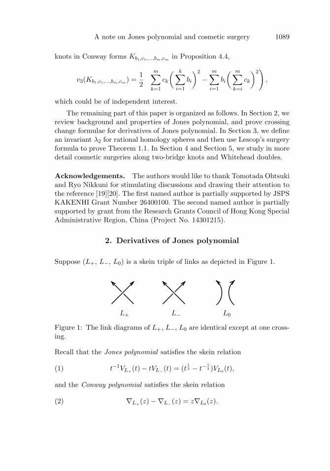
Suppose (L+, L−, L0) is a skein triple of links as depicted in Figure 1.

3

image) of K. We use the Alexander-Briggs notation and the Rolfsen [Ro] tables to distinguish be-tween a knot and its obverse. “Projection” is the same as “diagram”, and this means a knot or linkdiagram. Diagrams are always assumed oriented.The symbol ✷ denotes the end or the absence of a proof. In latter case it is assumed to be evidentfrom the preceding discussion/references; else (and anyway) I’m grateful for any feedback.

2. Positive knots and Gauß sumsDefinition 2.1 The writhe is a number (±1), assigned to any crossing in a link diagram. A crossingas on figure 1(a), has writhe 1 and is called positive. A crossing as on figure 1(b), has writhe −1 andis called negative. A crossing is smoothed out by replacing it by the fragment on figure 1(c) (whichchanges the number of components of the link). A crossing as on figure 1(a) and 1(b) is smashed toa singularity (double point) by replacing it by the fragment on figure 1(d). A m-singular diagram is adiagram with m crossings smashed. A m-singular knot is an immersion prepresented by a m-singulardiagram.

(a) (b) (c) (d)

Figure 1

Definition 2.2 A knot is called positive, if it has a positive diagram, i. e. a diagram with all crossingspositive.

Recall [FS, PV] the concept of Gauß sum invariants. As they will be the main tool of all the furtherinvestigations, we summarize for the benefit of the reader the basic points of this theory.

Definition 2.3 ([Fi3, PV]) A Gauß diagram (GD) of a knot diagram is an oriented circle with arrowsconnecting points on it mapped to a crossing and oriented from the preimage of the undercrossing tothe preimage of the overcrossing. See figure 2.

12

34

5

61

2

3

4

5

6

Figure 2: The knot 62 and its Gauß diagram.

Fiedler [Fi3, FS] found the following formula for (a variation of) the degree-3-Vassiliev invariantusing Gauß sums.

v3 = ∑(3,3)

wpwqwr + ∑(4,2)0

wpwqwr +12 ∑p,q linked

(wp+wq) , (1)

L+ L− L0

Figure 1: The link diagrams of L+, L−, L0 are identical except at one cross-ing.

Recall that the Jones polynomial satisfies the skein relation

(1) t−1VL+(t)− tVL−(t) = (t

1

2 − t− 1

2 )VL0(t),

and the Conway polynomial satisfies the skein relation

(2) ∇L+(z)−∇L−(z) = z∇L0

(z).

“3-Wu” — 2019/10/30 — 23:55 — page 1090 — #4


The normalized Alexander polynomial ∆L(t) is obtained by substitutingz = t1/2 − t−1/2 into the Conway polynomial. All these polynomial invariantsare defined to be the constant function 1 for the trivial knot.

For a knot K, let a2(K) be the coefficient of the z2-term of the Conwaypolynomial ∇K(z). From the fact that ∆′K(1) = 0, it is not hard to see that∆′′K(1) = 2a2(K). If one differentiates Equations (1) and (2) twice and com-pares the corresponding terms, one can also show that V ′′K(1) = −6a2(K).See [17] for details. In summary, we have:

Lemma 2.1. For all knots K ⊂ S3,

V ′′K(1) = −6a2(K) = −3∆′′K(1).

In [16], Lescop defined an invariant w3 for a knot K in a homology sphereY . When Y = S3, the knot invariant w3 satisfies a crossing change formula

w3(K+)− w3(K−) =a2(K

′) + a2(K′′)

2(3)

− a2(K+) + a2(K−) + lk2(K ′,K ′′)4

,

where (K+,K−,K ′ ∪K ′′) is a skein triple consisting of two knots K± anda two-component link K ′ ∪K ′′ [16, Proposition 7.2]. Clearly, the values ofw3(K) are uniquely determined by this crossing change formula once we fixw3(= 0) for the unknot. This gives an alternative characterization of theinvariant w3 for knots in S3. The next lemma relates it to the derivatives ofJones polynomial.

Lemma 2.2. For all knots K ⊂ S3,

w3(K) =1

72V ′′′K (1) +

1

24V ′′K(1).

Proof. The main argument essentially follows from Nikkuni [19, Proposition4.2]. We prove the lemma by showing that 1

72V′′′K (1) + 1

24V′′K(1) satisfies an

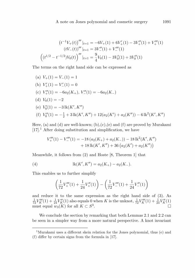
identical crossing change formula as Equation (3). To this end, we differenti-ate the skein formula for the Jones polynomial (1) three times and evaluateat t = 1. Abbreviating the Jones polynomial of the skein triple L+ = K+,L− = K− and L0 = K ′ ∪K ′′ by V+(t), V−(t) and V0(t), respectively, we ob-tain

“3-Wu” — 2019/10/30 — 23:55 — page 1091 — #5


(t−1V+(t)

)′′′ |t=1 = −6V+(1) + 6V ′+(1)− 3V ′′+(1) + V ′′′+ (1)

(tV−(t))′′′ |t=1 = 3V ′′−(1) + V ′′′− (1)(

(t1/2 − t−1/2)V0(t))′′′|t=1 =

9

4V0(1)− 3V ′0(1) + 3V ′′0 (1)

The terms on the right hand side can be expressed as

(a) V+(1) = V−(1) = 1

(b) V ′+(1) = V ′−(1) = 0

(c) V ′′+(1) = −6a2(K+), V ′′−(1) = −6a2(K−)

(d) V0(1) = −2

(e) V ′0(1) = −3 lk(K ′,K ′′)

(f) V ′′0 (1) = −12 + 3 lk(K ′,K ′′) + 12(a2(K

′) + a2(K′′))− 6 lk2(K ′,K ′′)

Here, (a) and (d) are well-known; (b),(c),(e) and (f) are proved by Murakami[17].1 After doing substitution and simplification, we have

V ′′′+ (1)− V ′′′− (1) = −18 (a2(K+) + a2(K−))− 18 lk2(K ′,K ′′)

+ 18 lk(K ′,K ′′) + 36(a2(K

′) + a2(K′′))

Meanwhile, it follows from (2) and Hoste [8, Theorem 1] that

(4) lk(K ′,K ′′) = a2(K+)− a2(K−).

This enables us to further simplify(

1

72V ′′′+ (1) +

1

24V ′′+(1)

)−(

1

72V ′′′− (1) +

1

24V ′′−(1)

)

and reduce it to the same expression as the right hand side of (3). As172V

′′′K (1) + 1

24V′′K(1) also equals 0 when K is the unknot, 1

72V′′′K (1) + 1

24V′′K(1)

must equal w3(K) for all K ⊂ S3. �

We conclude the section by remarking that both Lemmas 2.1 and 2.2 canbe seen in a simpler way from a more natural perspective. A knot invariant

1Murakami uses a different skein relation for the Jones polynomial, thus (e) and(f) differ by certain signs from the formula in [17].

“3-Wu” — 2019/10/30 — 23:55 — page 1092 — #6


v is called a finite type invariant of order n if it can be extended to aninvariant of singular knots via a skein relation

v(K) = v(K+)− v(K−)

where K is the knot with a transverse double point (See Figure 2), while vvanishes for all singular knots with (n+ 1) or more singularities.

3

image) of K. We use the Alexander-Briggs notation and the Rolfsen [Ro] tables to distinguish be-tween a knot and its obverse. “Projection” is the same as “diagram”, and this means a knot or linkdiagram. Diagrams are always assumed oriented.The symbol ✷ denotes the end or the absence of a proof. In latter case it is assumed to be evidentfrom the preceding discussion/references; else (and anyway) I’m grateful for any feedback.

2. Positive knots and Gauß sumsDefinition 2.1 The writhe is a number (±1), assigned to any crossing in a link diagram. A crossingas on figure 1(a), has writhe 1 and is called positive. A crossing as on figure 1(b), has writhe −1 andis called negative. A crossing is smoothed out by replacing it by the fragment on figure 1(c) (whichchanges the number of components of the link). A crossing as on figure 1(a) and 1(b) is smashed toa singularity (double point) by replacing it by the fragment on figure 1(d). A m-singular diagram is adiagram with m crossings smashed. A m-singular knot is an immersion prepresented by a m-singulardiagram.

(a) (b) (c) (d)

Figure 1

Definition 2.2 A knot is called positive, if it has a positive diagram, i. e. a diagram with all crossingspositive.

Recall [FS, PV] the concept of Gauß sum invariants. As they will be the main tool of all the furtherinvestigations, we summarize for the benefit of the reader the basic points of this theory.

Definition 2.3 ([Fi3, PV]) A Gauß diagram (GD) of a knot diagram is an oriented circle with arrowsconnecting points on it mapped to a crossing and oriented from the preimage of the undercrossing tothe preimage of the overcrossing. See figure 2.

12

34

5

61

2

3

4

5

6

Figure 2: The knot 62 and its Gauß diagram.

Fiedler [Fi3, FS] found the following formula for (a variation of) the degree-3-Vassiliev invariantusing Gauß sums.

v3 = ∑(3,3)

wpwqwr + ∑(4,2)0

wpwqwr +12 ∑p,q linked

(wp+wq) , (1)

Figure 2: a transverse double point in the singular knot K.

It follows readily from the definition that the set of finite type invariantsof order at most 1 consists of all constant functions. One can also showthat a2(K) and V ′′K(1) are finite type invariants of order 2, while w3(K)and V ′′′K (1) are finite type invariants of order 3. As the dimension of theset of all finite type invariants of order ≤ 2 and ≤ 3 are two and three,respectively (see, e.g., [2]), there has to be a linear dependence among theabove knot invariants, from which one can easily deduce Lemma 2.1 andLemma 2.2. In fact, if we denote v2 and v3 the finite type invariants of order2 and 3 respectively normalized by the conditions that v2(m(K)) = v2(K)and v3(m(K)) = −v3(K) for any knot K and its mirror image m(K) andthat v2(31) = v3(31) = 1 for the right hand trefoil 31, then it is not difficultto see that

(5) v2(K) = a2(K)

and

(6) v3(K) = −2w3(K).

3. Lescop invariant and cosmetic surgery

The goal of this section is to prove Theorem 1.1. First, recall the followingresults about purely cosmetic surgery from work of [3], [22], [26] and [18].

Theorem 3.1. Suppose K is a nontrivial knot in S3, r, r′ ∈ Q ∪ {∞} aretwo distinct slopes such that S3

r (K) ∼= S3r′(K) as oriented manifolds. Then

the following assertions are true:

“3-Wu” — 2019/10/30 — 23:55 — page 1093 — #7


(a) ∆′′K(1) = 0.

(b) r = −r′.(c) If r = p/q, where p, q are coprime integers, then q2 ≡ −1 (mod p).

(d) τ(K) = 0, where τ is the concordance invariant defined by Ozsvath-Szabo [21] and Rasmussen [23].

Our new input for the cosmetic surgery problem is Lescop’s λ2 invariantwhich, roughly speaking, is the degree 2 part of the Kontsevich-Kuperberg-Thurston invariant of rational homology spheres [16]. Like the famous Le-Murakami-Ohtsuki invariant, the Kontsevich-Kuperberg-Thurston invariantis universal among finite type invariants for homology spheres [13][14][15].See also Ohtsuki [20] for the connection to perturbative and quantum in-variants of three-manifolds.

We briefly review the construction. A Jacobi diagram is a graph withoutsimple loop whose vertices all have valency 3. The degree of a Jacobi diagramis defined to be half of the total number of vertices of the diagram. If wedenote byAn the vector space generated by degree n Jacobi diagrams subjectto some relations, then the degree n part Zn of the Kontsevich-Kuperberg-Thurston invariant takes its value in An.

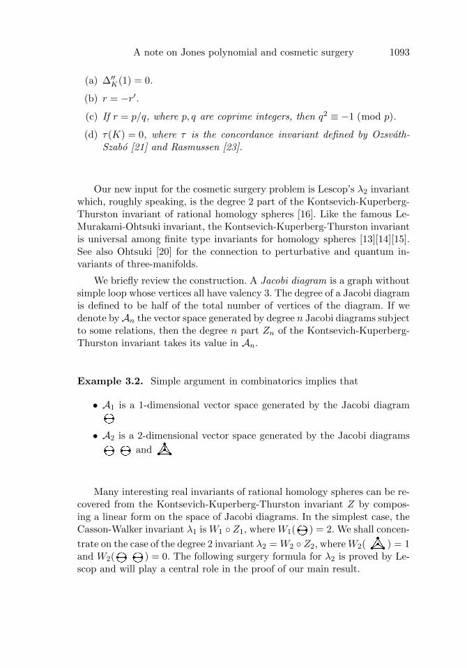
Example 3.2. Simple argument in combinatorics implies that

• A1 is a 1-dimensional vector space generated by the Jacobi diagram

• A2 is a 2-dimensional vector space generated by the Jacobi diagrams

and

Many interesting real invariants of rational homology spheres can be re-covered from the Kontsevich-Kuperberg-Thurston invariant Z by compos-ing a linear form on the space of Jacobi diagrams. In the simplest case, theCasson-Walker invariant λ1 is W1 ◦ Z1, where W1( ) = 2. We shall concen-

trate on the case of the degree 2 invariant λ2 = W2 ◦ Z2, whereW2( ) = 1and W2( ) = 0. The following surgery formula for λ2 is proved by Le-scop and will play a central role in the proof of our main result.

“3-Wu” — 2019/10/30 — 23:55 — page 1094 — #8


Theorem 3.3. [16, Theorem 7.1] The invariant λ2 satisfies the surgeryformula

λ2(Yp/q(K))−λ2(Y ) = λ′′2(K)

(q

p

)2

+w3(K)q

p+a2(K)c(q/p)+λ2(L(p, q))

for all knots K in a rational homology sphere Y .

Here, a2(K) is the z2-coefficient of ∇K(z), and L(p, q) is the lens spaceobtained by p/q surgery on the unknot.2 Then w3(K) is a knot invariant,which was shown earlier in Lemma 2.2 to be equal to 1

72V′′′K (1) + 1

24V′′K(1)

for K ⊂ S3. The terms λ′′2(K) and c(q/p) are both explicitly defined in [16],but they will not be needed for our purpose. For the moment, we make thefollowing simple observation.

Proposition 3.4. Suppose K is a knot in S3 with a2(K) = 0, and p, q arenonzero integers satisfying q2 ≡ −1 (mod p). Then

λ2(S3p/q(K)) = λ2(S

3−p/q(K))

if and only if w3(K) = 0.

Proof. We apply the surgery formula in Theorem 3.3. With the assumptionof a2(K) = 0, we can easily see that the first and third terms of the righthand side are equal for p/q and −p/q surgery, even without using knowledgeof λ′′2(K) or c(q/p). Next, recall the well-known theorem that two lens spacesL(p, q1) and L(p, q2) are equivalent up to orientation-preserving homeomor-phisms if and only if q1 ≡ q±12 (mod p). In particular, this implies the lensspaces L(p, q) ∼= L(p,−q) as oriented manifolds if q2 ≡ −1 (mod p), so theirλ2 invariants are obviously the same. Consequently,

λ2(S3p/q(K))− λ2(S3

−p/q(K)) = w3(K)2q

p,

and the statement follows readily. �

Proof of Theorem 1.1. In light of Theorem 3.1, we only need to considerthe case when ∆′′K(1) = 0 and q2 ≡ −1 (mod p), for otherwise, the pairof manifolds S3

p/q(K) and S3−p/q(K) will be non-homeomorphic as oriented

manifolds. Thus V ′′K(1) = −3∆′′K(1) = 0. If we now assume V ′′′K (1) 6= 0, then

2We use a different sign convention of lens spaces from Lescop’s original paper.

“3-Wu” — 2019/10/30 — 23:55 — page 1095 — #9


Lemma 2.2 implies that w3(K) 6= 0. We can then apply Proposition 3.4and conclude that λ2(S

3p/q(K)) 6= λ2(S

3−p/q(K)). Consequently, S3

p/q(K) �S3−p/q(K). �

Given (5) and (6), Theorem 1.1 can be stated in the following equivalentway, which is particularly useful in the case where it is easier to calculatethe finite type invariant v3 (or equivalently w3) than the Jones polynomial.

Theorem 3.5. If a knot K has the finite type invariant v2(K) 6= 0 orv3(K) 6= 0, then S3

r (K) � S3r′(K) for any two distinct slopes r and r′.

4. Examples of two-bridge knots

In this section, we derive an explicit formula for v3 and use it to study thecosmetic surgery problem for two-bridge knots. Following the presentation of[10, Section 2.1], we sketch the basic properties and notations for two-bridgeknots.

Every two-bridge knot can be represented by a rational number −1 <βα < 1 for some odd integer α and even integer β. If we write the reciprocalof this number as a continued fraction with even entries and of even length

α

β= [2b1, 2c1, . . . , 2bm, 2cm] = 2b1 +

1

2c1 +1

· · ·+ 1

2bm +1

2cm

for some nonzero integers bi’s and ci’s,3 then we obtain the Conway form

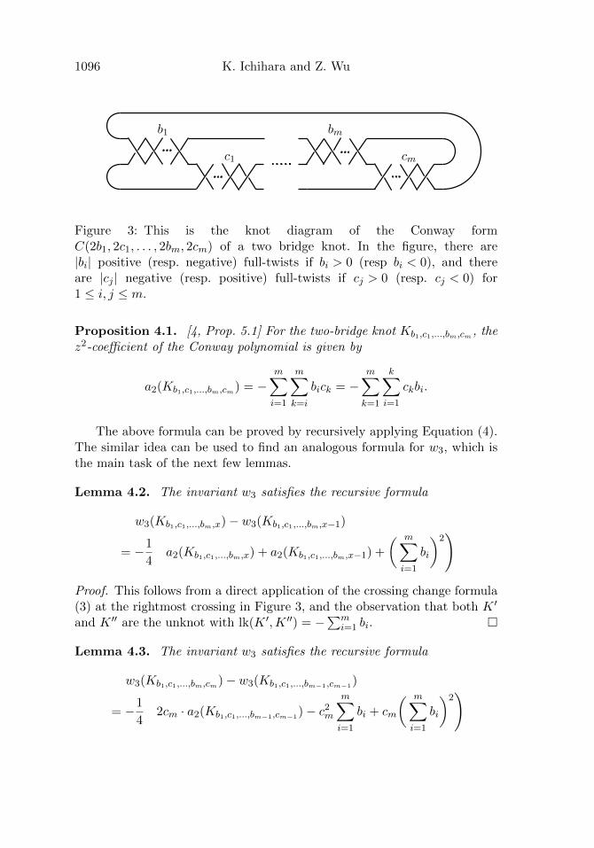
C(2b1, 2c1, . . . , 2bm, 2cm) of the two-bridge knot, which is a special knotdiagram as depicted in Figure 3. We will write Kb1,c1,...,bm,cm for the knotof Conway form C(2b1, 2c1, . . . , 2bm, 2cm). The genus of Kb1,c1,...,bm,cm is m;and conversely, every two-bridge knot of genus m has such a representation.

Burde obtained the following formula for a2(Kb1,c1,...,bm,cm), the z2-coefficient of the Conway polynomial of Kb1,c1,...,bm,cm .

3Such a representation always exists by elementary number theory.

“3-Wu” — 2019/10/30 — 23:55 — page 1096 — #10

1096 K. Ichihara and Z. Wu8 KAZUHIRO ICHIHARA AND ZHONGTAO WU

b1 bm

c1 cm

Figure 3. This is the knot diagram of the Conway formC(2b1, 2c1, · · · , 2bm, 2cm) of a two bridge knot. In the figure, there are|bi| positive (resp. negative) full-twists if bi > 0 (resp bi < 0), and there are |cj |negative (resp. positive) full-twists if cj > 0 (resp. cj < 0) for 1 ≤ i, j ≤ n.

Burde obtained the following formula for a2(Kb1,c1,··· ,bm,cm), the z2-coefficient of the Conwaypolynomial of Kb1,c1,··· ,bm,cm .

Proposition 4.1. [4, Proposition 5.1] For the two-bridge knot Kb1,c1,··· ,bm,cm, the z2-coefficientof the Conway polynomial is given by

a2(Kb1,c1,··· ,bm,cm) = −m∑

i=1

m∑

k=i

bick = −m∑

k=1

k∑

i=1

ckbi.

The above formula can be proved by recursively applying Equation (4). The similar idea canbe used to find an analogous formula for w3, which is the main task of the next few lemmas.

Lemma 4.2. The invariant w3 satisfies the recursive formula

w3(Kb1,c1,··· ,bm,x) − w3(Kb1,c1,··· ,bm,x−1)

= −1

4

(a2(Kb1,c1,··· ,bm,x) + a2(Kb1,c1,··· ,bm,x−1) + (

m∑

i=1

bi)2

)

Proof. This follows from a direct application of the crossing change formula (3) at the rightmostcrossing in Figure 3, and the observation that both K ′ and K ′′ are the unknot with lk(K ′,K ′′) =−∑m

i=1 bi.

�Lemma 4.3. The invariant w3 satisfies the recursive formula

w3(Kb1,c1,··· ,bm,cm) − w3(Kb1,c1,··· ,bm−1,cm−1)

= −1

4

(2cm · a2(Kb1,c1,··· ,bm−1,cm−1) − c2

m

m∑

i=1

bi + cm(m∑

i=1

bi)2

)

Proof. We first prove the lemma for cm > 0. We repeatedly apply Lemma 4.2 until x is reducedto 0. Note that the knot Kb1,c1,··· ,bm,0 can be isotoped to Kb1,c1,··· ,bm−1,cm−1 by untwisting thefar-right bm full twists. Therefore,

Figure 3: This is the knot diagram of the Conway formC(2b1, 2c1, . . . , 2bm, 2cm) of a two bridge knot. In the figure, there are|bi| positive (resp. negative) full-twists if bi > 0 (resp bi < 0), and thereare |cj | negative (resp. positive) full-twists if cj > 0 (resp. cj < 0) for1 ≤ i, j ≤ m.

Proposition 4.1. [4, Prop. 5.1] For the two-bridge knot Kb1,c1,...,bm,cm, thez2-coefficient of the Conway polynomial is given by

a2(Kb1,c1,...,bm,cm) = −m∑

i=1

m∑

k=i

bick = −m∑

k=1

k∑

i=1

ckbi.

The above formula can be proved by recursively applying Equation (4).The similar idea can be used to find an analogous formula for w3, which isthe main task of the next few lemmas.


w3(Kb1,c1,...,bm,x)− w3(Kb1,c1,...,bm,x−1)

= −1

4

(a2(Kb1,c1,...,bm,x) + a2(Kb1,c1,...,bm,x−1) +

( m∑

i=1

bi

)2)

Proof. This follows from a direct application of the crossing change formula(3) at the rightmost crossing in Figure 3, and the observation that both K ′

and K ′′ are the unknot with lk(K ′,K ′′) = −∑mi=1 bi. �


w3(Kb1,c1,...,bm,cm)− w3(Kb1,c1,...,bm−1,cm−1)

= −1

4

(2cm · a2(Kb1,c1,...,bm−1,cm−1

)− c2mm∑

i=1

bi + cm

( m∑

i=1

bi

)2)

“3-Wu” — 2019/10/30 — 23:55 — page 1097 — #11


Proof. We first prove the lemma for cm > 0. We repeatedly apply Lemma4.2 until x is reduced to 0. Note that the knot Kb1,c1,...,bm,0 can be isotopedto Kb1,c1,...,bm−1,cm−1

by untwisting the far-right bm full twists. Therefore,

w3(Kb1,c1,...,bm,cm)− w3(Kb1,c1,...,bm−1,cm−1)

= −1

4

(a2(Kb1,c1,...,bm,cm) + 2

cm−1∑

x=1

a2(Kb1,c1,...,bm,x)

+ a2(Kb1,c1,...,bm−1,cm−1) + cm

( m∑

i=1

bi

)2)

Now, the lemma follows from substituting

a2(Kb1,c1,...,bm,x) = a2(Kb1,c1,...,bm−1,cm−1)− x

m∑

i=1

bi,

which is an immediate corollary of Proposition 4.1.

The case when cm < 0 is proved analogously. �

Finally, applying Lemma 4.3 and induction on m, we obtain an explicitformula for w3, and consequently also for v3.

Proposition 4.4.

v3(Kb1,c1,...,bm,cm) = −2w3(Kb1,c1,...,bm,cm)

=1

2

(m∑

k=1

ck

( k∑

i=1

bi

)2

−m∑

i=1

bi

( m∑

k=i

ck

)2)

Proof. We use induction on m. For the base case m = 1, Lemma 4.3 readilyimplies that

w3(Kb1,c1) = −1

4(c1b

21 − c21b1),

so Kb1,c1 satisfies the formula.

Next we prove that if the formula holds for Kb1,c1,...,bm−1,cm−1, then it also

holds for Kb1,c1,...,bm,cm . It suffices to show that

“3-Wu” — 2019/10/30 — 23:55 — page 1098 — #12


− 1

4

(m∑

k=1

ck

( k∑

i=1

bi

)2

−m∑

i=1

bi

( m∑

k=i

ck

)2)

+1

4

(m−1∑

k=1

ck

( k∑

i=1

bi

)2

−m−1∑

i=1

bi

(m−1∑

k=i

ck

)2)

= −1

4

(2cm · a2(Kb1,c1,...,bm−1,cm−1

)− c2mm∑

i=1

bi + cm

( m∑

i=1

bi

)2)

where

a2(Kb1,c1,...,bm−1,cm−1) = −

m−1∑

i=1

m−1∑

k=i

bick.

The above identity can be verified from tedious yet elementary algebra. Weomit the computation here. �

For the rest of the section, we apply Theorem 3.5 and Proposition 4.4to study the cosmetic surgery problems for the two-bridge knots of genus 2and 3, which correspond to the Conway form Kb1,c1,b2,c2 and Kb1,c1,b2,c2,b3,c3 ,respectively. Note that the cosmetic surgery conjecture for genus one knotsis already settled by Wang [25].

Corollary 4.5. If a genus 2 two-bridge knot Kb1,c1,b2,c2 is not of the formKx,y,−x−y,x for some integers x, y, then it does not admit purely cosmeticsurgeries.

Proof. Suppose there are purely cosmetic surgeries for the knot Kb1,c1,b2,c2 .Theorem 3.5 implies that

(7) a2(Kb1,c1,b2,c2) = −(b1c1 + b1c2 + b2c2) = 0,

and

(8) v3(Kb1,c1,b2,c2) =1

2

(c1b

21 + c2(b1 + b2)

2 − b1(c1 + c2)2 − b2c22

)= 0,

where the formula for a2 and v3 follows from Propositions 4.1 and 4.4, re-spectively. From Equation (7), we see c2(b1 + b2) = −b1c1 and b1(c1 + c2) =−b2c2, which was then substituted into the second and the third terms of

“3-Wu” — 2019/10/30 — 23:55 — page 1099 — #13


Equation (8), and gives

v3(Kb1,c1,b2,c2) =1

2

(c1b

21 − b1c1(b1 + b2) + b2c2(c1 + c2)− b2c22

)

=1

2b2c1(c2 − b1) = 0.

Hence, b1 = c2. Plugging this identity back to Equation (7), we see b1 +b2 + c1 = 0. As a result, the two-bridge knot Kb1,c1,b2,c2 can be written asKx,y,−x−y,x for some integers x and y. �

We can perform a similar computation for a genus 3 two-bridge knotKb1,c1,b2,c2,b3,c3 . By Proposition 4.4,

v3(Kb1,c1,b2,c2,b3,c3) =1

2(c1b

21 + c2(b1 + b2)

2 + c3(b1 + b2 + b3)2

− b1(c1 + c2 + c3)2 − b2(c2 + c3)

2 − b3c23).

In particular, we see

v3(Kx,1,−x,x,1,−x) = −x 6= 0.

Consequently, Theorem 3.5 implies

Corollary 4.6. The family of two-bridge knots Kx,1,−x,x,1,−x, indexed byx ∈ Z− {0}, does not admit purely cosmetic surgeries.

Remark 4.7. As explained in [9], both ∆′′K(1) and τ(K) are 0 for theknot Kx,1,−x,x,1,−x. Hence, purely cosmetic surgery could not be ruled outby previously known results from Theorem 3.1.

5. Examples of Whitehead doubles

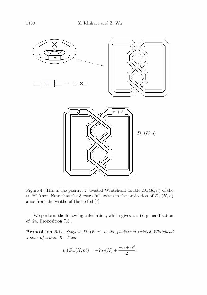
We are devoted to D+(K,n) in this section, where D+(K,n) denotes thesatellite of K for which the pattern is a positive-clasped twist knot with ntwists. The knot D+(K,n) is called the positive n-twisted Whitehead doubleof a knot K. See Figure 4 for an illustration.

“3-Wu” — 2019/10/30 — 23:55 — page 1100 — #14


n+ 3

D+(K,n)

Figure 4: This is the positive n-twisted Whitehead double D+(K,n) of thetrefoil knot. Note that the 3 extra full twists in the projection of D+(K,n)arise from the writhe of the trefoil [7].

We perform the following calculation, which gives a mild generalizationof [24, Proposition 7.3].

Proposition 5.1. Suppose D+(K,n) is the positive n-twisted Whiteheaddouble of a knot K. Then

v3(D+(K,n)) = −2a2(K) +−n+ n2

2.

“3-Wu” — 2019/10/30 — 23:55 — page 1101 — #15


In particular, for the untwisted Whitehead doubles D+(K, 0),

v3(D+(K, 0)) = −2a2(K).

Proof. We apply the crossing change formula (3) at either one of the cross-ings of the clasps. Note that K+ = D+(K,n), K− is the unknot, and K ′ =K ′′ = K. The classical formula for the Alexander polynomial of a satel-lite knot implies that ∆D+(K,n)(t) = −nt+ (2n+ 1)− nt−1, from which wecompute

a2(D+(K,n)) =1

2∆′′D+(K,n)(1) = −n.

Also observe that lk(K ′,K ′′) = −n. 4 Therefore,

w3(D+(K,n)) = a2(K)− −n+ n2

4,

and so

v3(D+(K,n)) = −2a2(K) +−n+ n2

2.

�

Since the invariant a2(D+(K,n)) = −n, the Whitehead doubleD+(K,n)does not admit purely cosmetic surgeries if n 6= 0. When n = 0, Proposi-tion 5.1 gives v3(D+(K,n)) = −2a2(K). Hence, Theorem 3.5 immediatelyimplies the following corollary.

Corollary 5.2. There is no purely cosmetic surgery for the positive n-twisted Whitehead double D+(K,n) for n 6= 0. Moreover, if a2(K) 6= 0, thenthere is no purely cosmetic surgery for the untwisted Whitehead doubleD+(K, 0).

Remark 5.3. Note that Whitehead doubles are genus 1 knots, so Corol-lary 5.2 also follows from Wang’s theorem [25, Theorem 1.3] that proved thenonexistence of cosmetic surgery for genus 1 knots.

References

[1] J. Baldwin and D. Gillam, Computations of Heegaard-Floer knot ho-mology, J. Knot Theory Ramifications 21 (2012), no. 8, 1250075, 65pp.

4This along with (4) gives an alternative way of seeing a2(D+(K,n)) = −n.

“3-Wu” — 2019/10/30 — 23:55 — page 1102 — #16


[2] D. Bar-Natan, On the Vassiliev knot invariants, Topology 34 (1995),no. 2, 423–472.

[3] S. Boyer and D. Lines, Surgery formulae for Casson’s invariant andextensions to homology lens spaces, J. Reine Angew. Math. 405 (1990),181–220.

[4] G. Burde, SU(2)-representation spaces for two-bridge knot groups,Math. Ann. 288 (1990), no. 1, 103–119.

[5] J. C. Cha and C. Livingston, KnotInfo: Table of Knot Invariants, http://www.indiana.edu/~knotinfo.

[6] C. Gordon, Dehn surgery on knots, in: Proceedings of the InternationalCongress of Mathematicians, Vol. I, II (Kyoto, 1990), pp. 631–642,Math. Soc. Japan, Tokyo.

[7] M. Hedden, Knot Floer homology of Whitehead doubles, Geom. Topol.11 (2007), 2277–2338.

[8] J. Hoste, The first coefficient of the Conway polynomial, Proc. Amer.Math. Soc. 95 (1985), no. 2, 299–302.

[9] K. Ichihara and T. Saito, Cosmetic surgery and the SL(2,C) Cassoninvariant for two-bridge knots, Hiroshima Math. J. 48 (2018), no. 1,21–37.

[10] A. Kawauchi, A Survey of Knot Theory, translated and revised fromthe 1990 Japanese original by the author, Birkhauser, Basel, (1996).

[11] R. Kirby, Problems in low-dimensional topology, in: Geometric topology(Athens, GA, 1993), pp. 35–473, AMS/IP Stud. Adv. Math., 2.2, Amer.Math. Soc., Providence, RI.

[12] The Knot Atlas, http://katlas.org/.

[13] M. Kontsevich, Feynman diagrams and low-dimensional topology, in:First European Congress of Mathematics, Vol. II (Paris, 1992), pp. 97–121, Progr. Math. 120, Birkhauser, Basel.

[14] G. Kuperberg and D. P. Thurston, Perturbative 3-manifold invariantsby cut-and-paste topology, arXiv:math/9912167.

[15] T. T. Q. Le, J. Murakami, and T. Ohtsuki, On a universal perturbativeinvariant of 3-manifolds, Topology 37 (1998), no. 3, 539–574.

http://www.indiana.edu/~knotinfo

http://www.indiana.edu/~knotinfo

http://katlas.org/

“3-Wu” — 2019/10/30 — 23:55 — page 1103 — #17


[16] C. Lescop, Surgery formulae for finite type invariants of rational ho-mology 3-spheres, Algebr. Geom. Topol. 9 (2009), no. 2, 979–1047.

[17] H. Murakami, On derivatives of the Jones polynomial, Kobe J. Math.3 (1986), no. 1, 61–64.

[18] Y. Ni and Z. Wu, Cosmetic surgeries on knots in S3, J. Reine Angew.Math. 706 (2015), 1–17.

[19] R. Nikkuni, Sharp edge-homotopy on spatial graphs, Rev. Mat. Com-plut. 18 (2005), no. 1, 181–207.

[20] T. Ohtsuki, Quantum Invariants, Series on Knots and Everything 29,World Sci. Publishing, River Edge, NJ, (2002).

[21] P. Ozsvath and Z. Szabo, Knot Floer homology and the four-ball genus,Geom. Topol. 7 (2003), 615–639.

[22] P. Ozsvath and Z. Szabo, Knot Floer homology and rational surgeries,Algebr. Geom. Topol. 11 (2011), no. 1, 1–68.

[23] J. Rasmussen, Floer homology and knot complements, Thesis (Ph.D.)–Harvard University, ProQuest LLC, Ann Arbor, MI, (2003), 126pp.

[24] A.Stoimenow, Positive knots, closed braids and the Jones polynomial,Ann. Sc. Norm. Super. Pisa Cl. Sci. (5) 2 (2003), no. 2, 237–285.

[25] J. Wang, Cosmetic surgeries on genus one knots, Algebr. Geom. Topol.6 (2006), 1491–1517.

[26] Z. Wu, Cosmetic surgeries on knots in S3, Geom. Topol. 15 (2011),1157–1168.

Department of Mathematics

College of Humanities and Sciences, Nihon University

3-25-40 Sakurajosui, Setagaya-ku, Tokyo 156-8550, Japan

E-mail address: [email protected]

Department of Mathematics

The Chinese University of Hong Kong

Shatin, Hong Kong

E-mail address: [email protected]

Received December 4, 2016

“3-Wu” — 2019/10/30 — 23:55 — page 1104 — #18


Accepted May 23, 2017

Documents

A note on Jones polynomial and cosmetic surgery