DRAFT

Cosmology, Theory and Observations

A note on large scale structures

Pierros Ntelis,a,1

aAix Marseille Univ, CNRS/IN2P3, Centre Physique de Particule a Marseille (CPPM), Mar-seille, France

E-mail: pntelis -at- cppm.in2p3.fr

Abstract. In this review, we present the basic concepts of physics on large scale structures.We start by giving a brief overview on the thermal history of our universe. We describe thetheoretical framework, behind the magnificent scenery of observations, known as the standardΛCDM model. The statistical observables currently used from surveys are discussed. We givean overview of the main limitation we have from observations. A summary of current andfuture large scale structure surveys is discussed. Finally, we give a brief overview on elementsof statistics needed to study large scale structures physics.

DRAFT

– i –

DRAFT

Contents

1 A brief introduction 22 An non exhaustive historical summary 33 Theoretical Framework 6

3.1 Smooth Cosmology 63.2 Perturbed Cosmology 93.3 Theoretical prediction 10

4 How our universe is structured? 115 Baryon Acoustic Oscillation: Briefly 136 Observations: Clustering statistics 14

6.1 The number overdensity field or density contrast 146.2 The two point correlation function 146.3 The power spectrum 166.4 Fractal Dimension 176.5 Anisotropic statistics 176.6 Higher order statistics 186.7 Non-Gaussianity 196.8 Estimators for Correlation function and Fractal Dimension 19

7 Limits on information mining 207.1 Causal diagrams 217.2 Cosmic Bias 227.3 Redshift Space Distortions 23

8 Large scale structure surveys, status 259 Statistical inference 26

9.1 Bayesian vs Frequentist 279.2 Bayesian Framework 289.3 Statistical indeference problem 299.4 First level inference: parameter estimation 299.5 Example 1 309.6 Example 2 319.7 Second level inference: model comparison 319.8 Example 3 339.9 MCMC parameter exploration 349.10 Basic Algorithm 349.11 Tests of MCMC convergence 35

10 Summary & Conclusion 36

– 1 –

DRAFT

1 A brief introduction

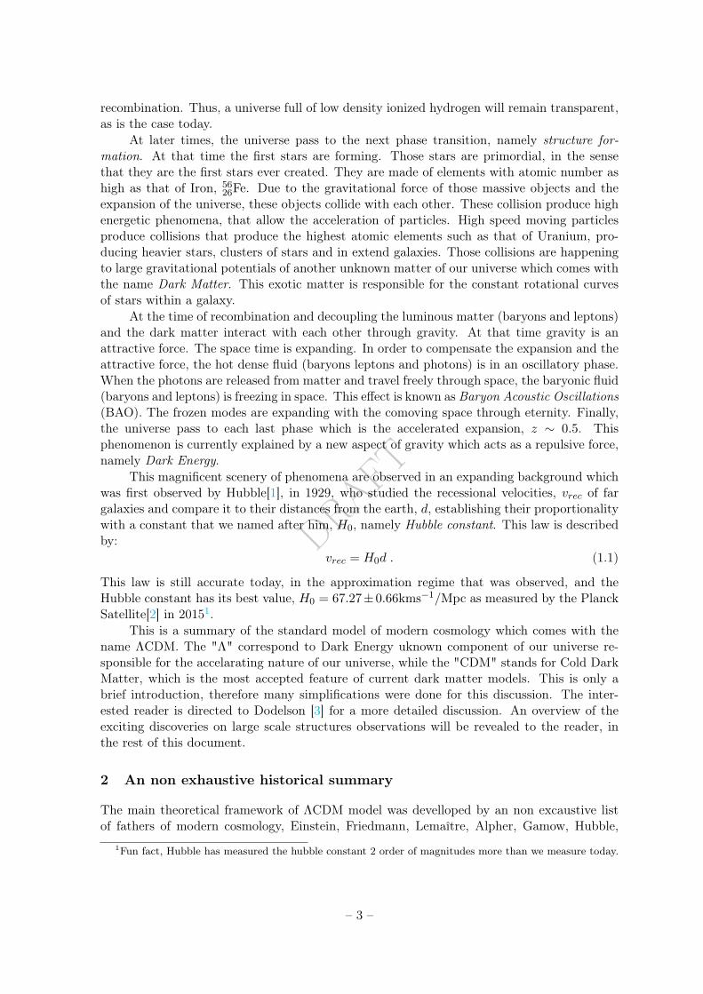
At first glance, we understand our universe as describe by Fig. 1. The universe starts fromquantum fluctuations, for unknown reasons, as a hot dense plasma at about 13.8 Gyrs ago.The interaction between baryons, leptons, photons, and neutrini is violent. An inflationarygrowth of structure follows only after 10−32sec after the "Big Bang". The photons are scatterfrom electrons and baryons and the universe is opaque. At about 380,000 yrs after the "BigBang", the interactions of photons, baryons and leptons reduce rapidly during an epoch knowas Big Bang Nucleonsynthesis (BBN). Therefore the photons are decoupled from the baryonsand leptons and start to diffuse freely in space at an epoch know as decoupling. This releasedradiation can be observed today. It is named as Cosmic Microwave Background (CMB). Atthat time baryons and leptons combined with each other to form the first neutral hydrogenatoms at an epoch known as recombination, z ∼ 1090. Due to the high transparency ofstructures and the fact that baryons and electrons do not interact with the photons, photonswere diffused rapidly into the spacetime continuum. Furthermore, there is an epoch of ouruniverse where matter does not interact with the light so we cannot observe it. Since, wehave no clue about the aforementioned epoch we named it, Dark Ages.

Figure 1. The current understanding of our universe. The universe starts as a hot densed fluid thatexpands through space for about 13.8 billion years. [See text for details]

About 400 million yrs after the "Big Bang" another phase change occurs, with the namereionisation epoch. At that time objects started to condense and become energetic enough toreionize neutral hydrogen. As these objects formed and radiated energy, the universe revertedfrom being neutral, to once again being an ionized plasma. This occurred between 150 millionand one billion years after the Big Bang, i.e. in terms of redshift, 6 < z < 20. At thattime, however, matter had been diffused by the expansion of the universe, and the scatteringinteractions of photons and electrons were much less frequent than before the lepton-baryon

– 2 –

DRAFT

recombination. Thus, a universe full of low density ionized hydrogen will remain transparent,as is the case today.

At later times, the universe pass to the next phase transition, namely structure for-mation. At that time the first stars are forming. Those stars are primordial, in the sensethat they are the first stars ever created. They are made of elements with atomic number ashigh as that of Iron, 56

26Fe. Due to the gravitational force of those massive objects and theexpansion of the universe, these objects collide with each other. These collision produce highenergetic phenomena, that allow the acceleration of particles. High speed moving particlesproduce collisions that produce the highest atomic elements such as that of Uranium, pro-ducing heavier stars, clusters of stars and in extend galaxies. Those collisions are happeningto large gravitational potentials of another unknown matter of our universe which comes withthe name Dark Matter. This exotic matter is responsible for the constant rotational curvesof stars within a galaxy.

At the time of recombination and decoupling the luminous matter (baryons and leptons)and the dark matter interact with each other through gravity. At that time gravity is anattractive force. The space time is expanding. In order to compensate the expansion and theattractive force, the hot dense fluid (baryons leptons and photons) is in an oscillatory phase.When the photons are released from matter and travel freely through space, the baryonic fluid(baryons and leptons) is freezing in space. This effect is known as Baryon Acoustic Oscillations(BAO). The frozen modes are expanding with the comoving space through eternity. Finally,the universe pass to each last phase which is the accelerated expansion, z ∼ 0.5. Thisphenomenon is currently explained by a new aspect of gravity which acts as a repulsive force,namely Dark Energy.

This magnificent scenery of phenomena are observed in an expanding background whichwas first observed by Hubble[1], in 1929, who studied the recessional velocities, vrec of fargalaxies and compare it to their distances from the earth, d, establishing their proportionalitywith a constant that we named after him, H0, namely Hubble constant. This law is describedby:

vrec = H0d . (1.1)

This law is still accurate today, in the approximation regime that was observed, and theHubble constant has its best value, H0 = 67.27±0.66kms−1/Mpc as measured by the PlanckSatellite[2] in 20151.

This is a summary of the standard model of modern cosmology which comes with thename ΛCDM. The "Λ" correspond to Dark Energy uknown component of our universe re-sponsible for the accelarating nature of our universe, while the "CDM" stands for Cold DarkMatter, which is the most accepted feature of current dark matter models. This is only abrief introduction, therefore many simplifications were done for this discussion. The inter-ested reader is directed to Dodelson [3] for a more detailed discussion. An overview of theexciting discoveries on large scale structures observations will be revealed to the reader, inthe rest of this document.

2 An non exhaustive historical summary

The main theoretical framework of ΛCDM model was develloped by an non excaustive listof fathers of modern cosmology, Einstein, Friedmann, Lemaître, Alpher, Gamow, Hubble,

1Fun fact, Hubble has measured the hubble constant 2 order of magnitudes more than we measure today.

– 3 –

DRAFT

Zwicky, ... . Einstein developed the Theory of General Relativity in 1915[4] which explainshow gravity is only a manifestation of the effect of how the matter locally affects the curvatureof space time around it. This theory is formulated in the well know Einstein field equation

Gµν(x) = κTµν(x) , (2.1)

where Gµν is the Einstein tensor that describes the local curvature around a specific matterdensity which has a simplistic energy tensor, Tµν , and κ is a topological constant. In 1922,Friedmann[3] have applied the above formulation to a model for the evolution of the universe.He solved the above equations for a homogeneous and isotropic universe. At about thesame time independently, in 1931, Lemaitre applied the above equations for solutions of ahomogeneous and isotropic universe that starts from a small hot dense region known as the"Big Bang Theory". Notice that this term is inaccurate since the equations break down onr = 0, an issue know as singularity. However, this description agrees with the data that wehave so far, which are not corresponding to r = 0 and therefore this model is still well acceptedfrom the largest amount of the physics community, nowadays, 2019. This can be expressedas the smooth cosmology that we are going to briefly describe in section 3.1. However, thestandard model described by a "Big Bang" origin is still under investigation against theseveral attempts to explain some unexplained phenomena. Alternatives to this model areamong the following: Late time isotropic universe, Bouncing universe, Multiverse, and so on.

Fast forward in time, 1948, Alpher a student of Gamow with his supervisor have pre-dicted that the universe initially could emit a radiation at the Microwave regime known as theCosmic Microwave Background (CMB) radiation. That year they published2 the so calledα, β, γ-paper[5] . In 1965, Penzias and Wilson have observed by accident this radiation[6]without knowing the prediction of the Alpher and Gamow. Fast forward in time in 2006,Smooth and Mather got a Nobel Prize for the discovery of the Black Body nature of CMBby leading the team on observing with unprecedentedly accuracy the CMB temperature,TCMB = 2.728 ± 0.004 K as measured by the FIRAS instrument of COBE satellite[7]. Thismeasurement confirmed the state of the art ΛCDM model which predicts the Baryon Acous-tic Oscillation phenomenon behind the structure of the CMB radiation. Afterwards, WMAPconfirmed this oscillatory feature by studying the temperature fluctuations of the CMB in2010 [8]. Now the state of the art of this measurement is acquired by Planck satellite[2]measuring the CMB fluctuations with unprecedentedly accuracy, ∆T/T ∼ 10−5 at redshift,z ∼ 1090 and inferring precision measurement on the parameters of ΛCDM model amongalternatives.

In 1965, Gunn and Peterson observed the Gunn-Peterson trough, a feature of the spectraof quasars due to the presence of neutral hydrogen in the Intergalactic Medium (IGM) [9].This marked the epoch of reionisation which is a hot research area these days due to the lackof observations at 6 < z < 20.

In the field of large scale structure observations there were several developments as wellat that time. In 1929, Hubble[1] turned his telescope on the sky and observed the expansionof the universe confirming the theoretical framework build upon the previous authors. Hubbledetermined a linear relation between the recessional velocities (vrec) and the radial distancesof galaxies):

vrec := cz = H0d (2.2)

2They have introducing to the author list the friend of Gamow, Bethe. Bethe has nothing to do with thisresearch but he was selected on the author’s list by the authors only for the sake of the naming of the paper!

– 4 –

DRAFT

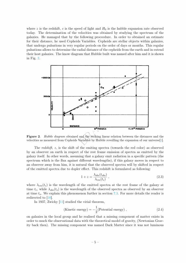
where z is the redshift, c is the speed of light and H0 is the hubble expansion rate observedtoday. The determination of the velocities was obtained by studying the spectrum of thegalaxies. He managed that by the following proceedure. In order to obtained an estimatefor their distance, he used Cepheids Variables. Cepheids are stellar objects within galaxies,that undergo pulsations in very regular periods on the order of days or months. This regularpulsations allows to determine the radial distance of the cepheids from the earth and in extendtheir host galaxies. The know diagram that Hubble built was named after him and it is shownin Fig. 2.

Figure 2. Hubble diagram obtained and the striking linear relation between the distances and thevelocities as measured from Cepheids Variables by Hubble reveilling the expansion of our universe[1].

The redshift, z, is the shift of the emiting spectra (towards the red color) as observedby an observer on earth in respect of the rest frame emission of spectra as emitted by thegalaxy itself. In other words, assuming that a galaxy emit radiation in a specific pattern (thespectrum which is the flux against different wavelengths), if this galaxy moves in respect toan observer away from him, it is nutural that the observed spectra will by shifted in respectof the emitted spectra due to dopler effect. This redshift is formulated as following:

1 + z =λobs(tobs)

λem(te), (2.3)

where λem(te) is the wavelength of the emitted spectra at the rest frame of the galaxy attime te, while λobs(to) is the wavelength of the observed spectra as observed by an observerat time to. We explain this phenomenon further in section 7.3. For more details the reader isredirected to [10].

In 1937, Zwicky [11] studied the virial theorem,

(Kinetic energy) = −1

2(Potential energy) , (2.4)

on galaxies in the local group and he realised that a missing compenent of matter exists inorder to much the observational data with the theoretical model of gravity, (Newtonian Grav-ity back then). The missing component was named Dark Matter since it was not luminous

– 5 –

DRAFT

but was interacting with the luminous matter through gravity. This missing matter couldcompensate the missing mass that was necessary to fit the constant rotational curves at largeradii away from the centers of the galaxies. A more robust confirmation of this phenomenonwas aqcuired later on by Ruby[12] in 1970, who studied the rotation of the andromeda nebulafrom a spectroscopic survey.

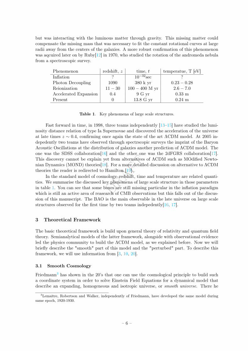
Phenomenon redshift, z time, t temperatue, T [eV]Inflation ? 10−32sec ?Photon Decoupling 1090 380 k yr 0.23− 0.28Reionization 11− 30 100− 400 M yr 2.6− 7.0Accelerated Expansion 0.4 9 G yr 0.33 mPresent 0 13.8 G yr 0.24 m

Table 1. Key phenomena of large scale structures.

Fast forward in time, in 1998, three teams independently [13–15] have studied the lumi-nosity distance relation of type Ia Supernovae and discovered the acceleration of the universeat late times z ∼ 0.4, confirming once again the state of the art ΛCDM model. At 2005 in-depedently two teams have observed through spectrscopic surveys the imprint of the BaryonAcoustic Oscillations at the distribution of galaxies another prediction of ΛCDM model. Theone was the SDSS collaboration[16] and the other one was the 2dFGRS collaboration[17].This discovery cannot be explain yet from alternatives of ΛCDM such as MOdified Newto-nian Dynamics (MOND) theories[18]. For a more detailed discussion on alternative to ΛCDMtheories the reader is redirected to Hamilton [19].

In the standard model of cosmology, redshift, time and temperature are related quanti-ties. We summarise the discussed key phenomena of large scale structure in those parametersin table 1. You can see that some boxes are still missing particular in the inflation paradigmwhich is still an active area of reasearch of CMB observations but this falls out of the discus-sion of this manuscript. The BAO is the main observable in the late universe on large scalestructures observed for the first time by two teams indepedently[16, 17].

3 Theoretical Framework

The basic theoretical framework is build upon general theory of relativity and quantum fieldtheory. Semianalytical models of the latter framework, alongside with observational evidenceled the physics community to build the ΛCDM model, as we explained before. Now we willbriefly describe the "smooth" part of this model and the "perturbed" part. To describe thisframework, we will use information from [3, 10, 20].

3.1 Smooth Cosmology

Friedmann3 has shown in the 20’s that one can use the cosmological principle to build sucha coordinate system in order to solve Einstein Field Equations for a dynamical model thatdescribe an expanding, homogeneous and isotropic universe, or smooth universe. There he

3Lemaître, Robertson and Walker, independently of Friedmann, have developed the same model duringsame epoch, 1920-1930.

– 6 –

DRAFT

showed that for a statistically homogeneous and isotropic universe, an observer has a coordi-nate system that follows the FLRW metric4:

ds2 = −c2dt2 + a2(t)

[1

1− krdr2 + r2(dθ2 + sin2θdφ2)

](3.1)

where dΩ = dθ2+sin2θdφ2 reflects the isotropy condition and γij = 11−kr2dr

2+r2dΩ describedthe radial condition of the metric. This metric defines an infinitely expanding universe. Theexpansion is quantified by the scale factor, a(t). If k = 0, space is Minkovskiy flat topology(flat). If 0 < k < 1 space is spherical topology (closed), while −1 < k < 0 correspond to ahyperbolic topology (open).

The FLRW metric is used as an input on the left hand side of equation Eq. 2.1 for thecomputation of the scale factor as a function of the topological properties of the universe.Thus one can easily show that the Einstein Tensor, for an FLRW metric (Eq. 3.1), reducesto a tensor with the following non-zero components:

G00 = 3

([a(t)

a(t)

]2

+kc2

a2(t)

), Gij = −γij

[k + 2a(t)a(t) + a2(t)

](3.2)

where dot " ˙ " represent the derivative in respect of time t.The right hand side of equation Eq. 2.1 describes the energy content of the universe as a

perfect fluid in thermodynamic equilibrium, thus the energy-stress tensor takes the simplifiedform:

Tµν =

[ρ(x) +

P (x)

c2

]uµuν + P (x)gµν (3.3)

where ρ(x) is the energy density, P (x) is the pressure and uµ is the 4-velocity. The cosmo-logical principle implies that uµ = (1, 0, 0, 0), meaning that the fluid is locally at rest withrespect to the chosen frame. Furthermore, the cosmological principle restricts the energydensity and pressure to be constant over space but allows a possible time dependence. Theseconsiderations model the stress energy tensor, with only non-zero components, as follows:

T00 = ρ(t), Tij =P (t)

c2a2(t)γij (3.4)

The gauge invariance allows us to add a constant on the Eq. 2.1, cosmological constant, Λ. Bytaking all the above considerations into account, the 00-component and the trace of Eq. 2.1are written as:

H2(t) ≡(a

a

)=

8πG

3ρ(t)− kc2

a2(t)+

Λc2

3(3.5)

−(a

a

)=

8πG

2

[ρ(t) +

3P (t)

c2

]− Λc2

3(3.6)

where the H(t) = a/a is the Hubble expansion rate at time t. The above differential equationsare not enough to completely specify the system, i.e. a(t), ρ(t) and P (t). Thus, either bycombining the above equations or by using the local conservation of the stress-energy tensor(Tµν;µ = 0), we have that:

ρ(t) = −3H(t)

[ρ(t) +

P (t)

c2

](3.7)

4For an approach that has more general considerations of topology on constructing this metric, see Ap-pendix A2: Topological Restrictions from Ntelis [10]

– 7 –

DRAFT

The set of the 3 latter equations (Eq. 3.5, Eq. 3.6 and Eq. 3.7) are used to describe theevolution a(t) of the cosmic fluid with properties ρ(t) and p(t). This set of equations arecalled Friedmann equations. However, in the ΛCDM-modelling there are several species ofthe total cosmic fluid such as X = γ, ν, b, cdm,Λ which corresponds to photons, baryons,neutrinos, cold dark matter and dark energy, respectively.

The cosmic species are divided into two general categories, i.e. the relativistic and nonrelativistic species, according to the level of their rest mass energy mc2. The former havea rest mass energy which is insignificant against their average kinetic energy mc2 << kBT .This leads to Prel = ρrel/3. The latter are those whose momentum is negligible to their restenergy (mc2 >> kBT ), and therefore Pn.rel ' 0. However, one may generalise those twoapproximated relations for the two categories of species with a parameter

w =P

ρc2(3.8)

namely equation of state parameter. This allow for a class of solutions of Eq. 3.7, i.e.

ρX(t) ∝ [a(t)]−3(wX+1) (3.9)

for each species X.It is convenient, now, to define the critical energy density as the energy density for a

universe of zero curvature (k=0) and no cosmological constant (Λ = 0):

ρc(t) =3H2(t)

8πG(3.10)

Then by dividing Eq. 3.5 with H2(t), we have:

1 =8πG

3H2(t)ρ(t)− kc28πG

8πGa2(t)H2(t)+

Λc28πG

3× 8πGH2(t)(3.11)

Now substituting Eq. 3.10 to Eq. 3.11 we have:

1 =ρ(t)

ρc(t)− 1

ρc(t)

kc2

8πGa2(t)+

1

ρc(t)

Λc2

3× 8πG(3.12)

Last but not least, we introduce the ratio of energy densities of the possible species (X) ofour universe against the critical density as:

ΩX(t) =ρX(t)

ρc(t)(3.13)

where X = γ, ν, b, cdm,Λ correspond to photons, baryons, neutrinos, cold dark matter anddark energy, respectively. One may define as well the energy density ratio of curvature as:

Ωk(t) = − kc2

8πGa2(t). (3.14)

Therefore, all those species must satisfy the local energy conservation equation at all times:

Ωk(t) +∑X

ΩX(t) = 1 . (3.15)

Thus in the field of concordance cosmology, we use the above simple parametrization (Eq. 3.13)to measure the ratio of energy densities of the different species in our universe. The conventionwe adopted is that when we drop the time dependence, we talk about the energy density ratiotoday ΩX = ΩX(t = 0).

– 8 –

DRAFT

3.2 Perturbed Cosmology

The latest observations, such as the CMB measurements[21], have shown that the universe isfull of small scale inhomogeneities. In other worlds the universe behaves not homogeneouslyat smaller scales. Two ingredients are necessary to describe the unforementioned inhomo-geneities. The first ingredient is the perturbation of the smooth metric, i.e. FLRW metric(Eq. 3.1). The second one is the Boltzmann equation that describe the nature of the interac-tions and the evolution between the different species of the cosmic fluid, beyond equilibrium.

In order to account for those small scale inhomogeneities in the previous described frame-work (section 3.1), we perform a perturbations in the metric. The mechanism of perturbationgive rise to a gauge-invariance. This is described by two different ways of takling this free-dom, the conformal Newtonian gauge and the synchronous gauge. However, the synchronousgauge has been advocated by Ma and Bertschinger [22] that Newtonian gauge is the simplestone and although it can eliminate the vector and tensor modes by definition, it can be easilygeneralised to include them. In our case, we are going to describe the simplest one, the New-tonian gauge with the scalar modes. Therefore, the FLRW metric in the perturbation theoryis going to be rewritten simply as:

ds2 = − [1 + 2Ψ(~x)] dt2 + a2(t) [1 + 2Φ(t)] d~x2 (3.16)

where we have considered scalar perturbations defined via the Φ(t) spatial curvature field andthe Ψ(~x) Newtonian potential field. By neglecting Ψ and Φ scalar perturbations, we retrievethe homogeneous and isotropic, FLRW metric.

The Perturbed Boltzmann Einstein Equations can be summarised symbolically as:

Dt [fX(~x, ~p, t)] = C [fX(~x, ~p, t)] (3.17)

where the left hand side describes the time evolution of the distribution fX(~x, ~p, t) of theprimordial fluctuations of each species, which we have developed in first order approximation.Note that in first order approximation we have that:

Dt = ∂t + a−1(t)pi + ∂tΦ(t) + a−1(t)pi∂iΨ(~x) (3.18)

which is the well defined derivative of the perturbed metric. The right hand side of Eq. 3.17describes the collision treatment between the different species X, C[fX ]. For the interactionbetween photons and leptons, we consider the classical Thomson scattering non-relativisticapproach, l∓ + γ ↔ l∓ + γ with an interaction rate Γ ' nlσT , where σT ' 2× 10−3MeV −2

is the Thomson cross section.For cold dark matter, we consider a collisionless non-relativistic approach, as done in

various famous structure formation history models. These are the simplest models that agreewith observational large scale structure data. For baryons and leptons interactions, we assumea Coulomb Scattering, b±+ l∓ ↔ b±+ l∓ in the Quantum ElectroDynamic (QED) approach.The neutrini are considered as a massless relativistic particle fluctuation overdensity andtherefore we assume that they do not interact with matter at first order. This is true onlyin the linear regime at large scales. Adopting a Fourier transform framework to simplify theequations in question, we end up with a set of 6 linear differential equations describing thenon linear evolution of the 3 different species of density fluctuations (baryons, photons andneutrinos and Dark Matter) and their corresponding velocities at large scale as a function of

– 9 –

DRAFT

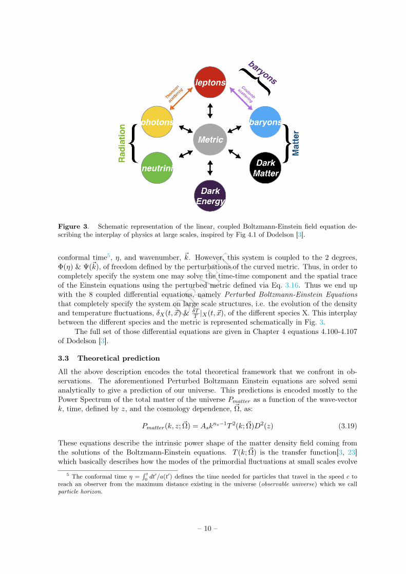
Figure 3. Schematic representation of the linear, coupled Boltzmann-Einstein field equation de-scribing the interplay of physics at large scales, inspired by Fig 4.1 of Dodelson [3].

conformal time5, η, and wavenumber, ~k. However, this system is coupled to the 2 degrees,Φ(η) & Ψ(~k), of freedom defined by the perturbations of the curved metric. Thus, in order tocompletely specify the system one may solve the time-time component and the spatial traceof the Einstein equations using the perturbed metric defined via Eq. 3.16. Thus we end upwith the 8 coupled differential equations, namely Perturbed Boltzmann-Einstein Equationsthat completely specify the system on large scale structures, i.e. the evolution of the densityand temperature fluctuations, δX(t, ~x) & δT

T |X(t, ~x), of the different species X. This interplaybetween the different species and the metric is represented schematically in Fig. 3.

The full set of those differential equations are given in Chapter 4 equations 4.100-4.107of Dodelson [3].

3.3 Theoretical prediction

All the above description encodes the total theoretical framework that we confront in ob-servations. The aforementioned Perturbed Boltzmann Einstein equations are solved semianalytically to give a prediction of our universe. This predictions is encoded mostly to thePower Spectrum of the total matter of the universe Pmatter as a function of the wave-vectork, time, defined by z, and the cosmology dependence, ~Ω, as:

Pmatter(k, z; ~Ω) = Askns−1T 2(k; ~Ω)D2(z) (3.19)

These equations describe the intrinsic power shape of the matter density field coming fromthe solutions of the Boltzmann-Einstein equations. T (k; ~Ω) is the transfer function[3, 23]which basically describes how the modes of the primordial fluctuations at small scales evolve

5 The conformal time η =∫ t

0dt′/a(t′) defines the time needed for particles that travel in the speed c to

reach an observer from the maximum distance existing in the universe (observable universe) which we callparticle horizon.

– 10 –

DRAFT

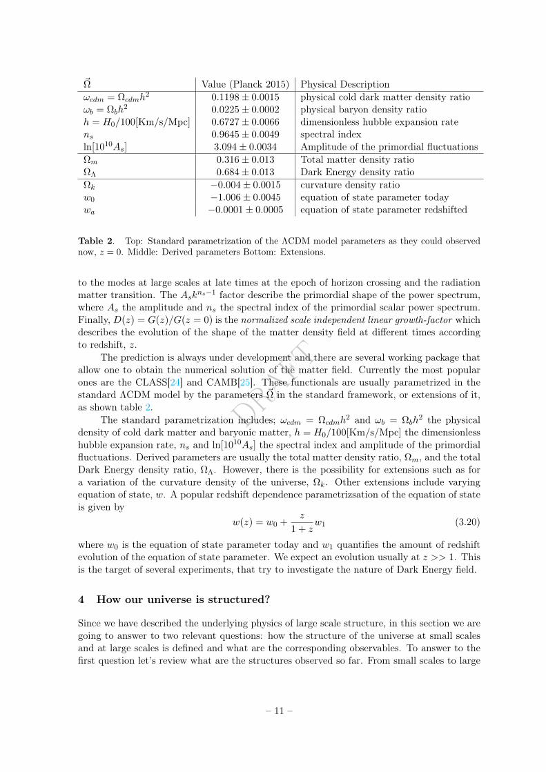
~Ω Value (Planck 2015) Physical Descriptionωcdm = Ωcdmh

2 0.1198± 0.0015 physical cold dark matter density ratioωb = Ωbh

2 0.0225± 0.0002 physical baryon density ratioh = H0/100[Km/s/Mpc] 0.6727± 0.0066 dimensionless hubble expansion ratens 0.9645± 0.0049 spectral indexln[1010As] 3.094± 0.0034 Amplitude of the primordial fluctuationsΩm 0.316± 0.013 Total matter density ratioΩΛ 0.684± 0.013 Dark Energy density ratioΩk −0.004± 0.0015 curvature density ratiow0 −1.006± 0.0045 equation of state parameter todaywa −0.0001± 0.0005 equation of state parameter redshifted

Table 2. Top: Standard parametrization of the ΛCDM model parameters as they could observednow, z = 0. Middle: Derived parameters Bottom: Extensions.

to the modes at large scales at late times at the epoch of horizon crossing and the radiationmatter transition. The Askns−1 factor describe the primordial shape of the power spectrum,where As the amplitude and ns the spectral index of the primordial scalar power spectrum.Finally, D(z) = G(z)/G(z = 0) is the normalized scale independent linear growth-factor whichdescribes the evolution of the shape of the matter density field at different times accordingto redshift, z.

The prediction is always under development and there are several working package thatallow one to obtain the numerical solution of the matter field. Currently the most popularones are the CLASS[24] and CAMB[25]. These functionals are usually parametrized in thestandard ΛCDM model by the parameters ~Ω in the standard framework, or extensions of it,as shown table 2.

The standard parametrization includes; ωcdm = Ωcdmh2 and ωb = Ωbh

2 the physicaldensity of cold dark matter and baryonic matter, h = H0/100[Km/s/Mpc] the dimensionlesshubble expansion rate, ns and ln[1010As] the spectral index and amplitude of the primordialfluctuations. Derived parameters are usually the total matter density ratio, Ωm, and the totalDark Energy density ratio, ΩΛ. However, there is the possibility for extensions such as fora variation of the curvature density of the universe, Ωk. Other extensions include varyingequation of state, w. A popular redshift dependence parametrizsation of the equation of stateis given by

w(z) = w0 +z

1 + zw1 (3.20)

where w0 is the equation of state parameter today and w1 quantifies the amount of redshiftevolution of the equation of state parameter. We expect an evolution usually at z >> 1. Thisis the target of several experiments, that try to investigate the nature of Dark Energy field.

4 How our universe is structured?

Since we have described the underlying physics of large scale structure, in this section we aregoing to answer to two relevant questions: how the structure of the universe at small scalesand at large scales is defined and what are the corresponding observables. To answer to thefirst question let’s review what are the structures observed so far. From small scales to large

– 11 –

DRAFT

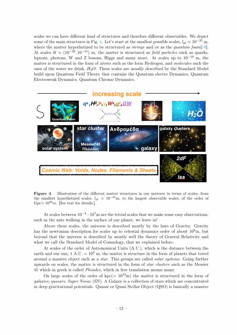
scales we can have different kind of structures and therefore different observables. We depictsome of the main structures in Fig. 4. Let’s start at the smallest possible scales, lpl ' 10−35 m,where the matter hypothetized to be structured as strings and/or as the quantum foam[10].At scales δl ' (10−20, 10−15) m, the matter is structured as field particles such as quarks,leptons, photons, W and Z bosons, Higgs and many more. At scales up to 10−10 m, thematter is structured in the form of atoms such as the form Hydrogen, and molecules such theones of the water we drink, H2O. These scales are usually described by the Standard Modelbuild upon Quantum Field Theory that contains the Quantum electro Dynamics, QuantumElectroweak Dynamics, Quantum Chromo Dynamics.

Figure 4. Illustration of the different matter structures in our universe in terms of scales, fromthe smallest hypothetized scales, lpl ' 10−35m, to the largest observable scales, of the order ofGpc' 1026m. [See text for details.]

At scales between 10−4−107m are the trivial scales that we make some easy observations,such as the ants walking in the surface of our planet, we leave in!

Above these scales, the universe is described mostly by the laws of Gravity. Gravityhas the newtonian description for scales up to celestial dynamics order of about 108m, butbeyond that the universe is described by mostly well the theory of General Relativity andwhat we call the Standard Model of Cosmology, that we explained before.

At scales of the order of Astronomical Units (A.U.), which is the distance between theearth and our sun, 1 A.U. = 109 m, the matter is structure in the form of planets that travelaround a massive object such as a star. This groups are called solar systems. Going furtherupwards on scales, the matter is structured in the form of star clusters such as the Messier45 which in greek is called Pleiades, which in free translation means many.

On large scales of the order of kpc(= 1019m) the matter is structured in the form ofgalaxies, quasars, Super Novae (SN). A Galaxy is a collection of stars which are concentratedin deep gravitational potentials. Quasar or Quasi Stellar Object (QSO) is basically a massive

– 12 –

DRAFT

galaxy that formed in the early universe6. Explosions of stars or galaxies in the late timeuniverse. Further classification includes galaxy clusters that are collections of galaxies in largegravitational potential at the order of few kpc. Do not forget that also there is the dark matterparticles that usually are invisible to our instruments but they are being traced by observingthe dynamics of the luminous matter such as the galaxies. At the largest possibly observablesscales, order of few Gpc(' 1026m), there are also some other classification. The structured canbe classified at the largest possible scales of the universe, in terms of Nodes, Filaments, Sheetsand Voids, namely Cosmic Web. Nodes are a massive collection of galaxies and star clusters inthe visinity of huge gravitational potentials. Due to the fact that the gravitational potentialhave tidal forces, the structures also form filaments which are basically long structures. Thesheets are due to the fact that the gravitational potential force the matter structures to havetwo dimensional shape with some thickness, that gives the shape of sheets that we use tocover at night below the magnificent scenery of stars on camping. This form of structure canbe also be consider as structure of foams. Therefore one can observe that at the very smallscales, infinitesimally small and at the very large scales, infinitesimally large , the universe isstructure as a foam, or namely large scale structure foam!

If one would like to describe marginally, the two structures towards the two infinities,he would give them a proper name, namely the cosmic scaling foam. The cosmic scaling foamis the form of structure at the infinitesimally small and the infinitesimally large scales of ouruniverse. In other words, one would say that the universe seems blurry at the two infinities!How we can optimally combine these observations to distinguish between models is still anopen question of current research!

The second question, what is our observable, is more complicated to answer. As youunderstood a structure can have different forms, and we can pick different ways to model itand study it according to our preference and convenience. On large scale structures, we areinterested on how matter is dynamically distributed. Therefore we are interested in the lightcoming from distant objects such as galaxies and the early universe (CMB radiation) which areable trace the total matter fluid of our universe. Therefore radiation in the form of photons isthe main observable that allows us to observe the largest possible scales. Additionally, we aregoing to treat galaxies as point source of photon radiation to study their statistical properties.

These objects helps to constrain our theoretical models of cosmology such as the standardΛCDM model or modifications of gravity and several submodels of this universal model suchas galaxy formation, Dark Energy models, Dark Matter models etc.

5 Baryon Acoustic Oscillation: Briefly

According to the previous short summary of our standard ΛCDM model, now we are able togive the insights of the famous phenomenon, Baryon Acoustic Oscillations.

About 300,000yr after the Big Bang, the universe was in a hot and dense state expandingrapidly. Baryons , leptons and photons were interacting with each other due to high tempera-ture. Note that the gravitational potential, which is created by the total matter, is attractive.While the kinetic energy coming from the high temperature and interaction of the particleswas high. This creates an outward pressure on the structures. These counteracting forcesof gravity and pressure created oscillations in the structure of total matter of the universe,analogous to the sound waves created in the air by pressure differences.

6Fun Fact! They were named Quasi Stellar Objects because at first they were identified as stars (hencestellar) with non similar fluxes (hence quasi)

– 13 –

DRAFT

At about ∼ 360, 000yr after the Big Bang (Recombination epoch), the universe coolsdown at a point were the baryons are combined with the leptons. These acoustic oscillationsalmost freeze in the spacetime continuum.

Shortly after, about ∼ 380, 000yr after Big Bang (Decoupling epoch), the photons cannotinteract anymore with the already produced atoms. Therefore the photons free stream intothe space-time continuum, in the form of CMB radiation. Note that the informations of BAOoscillations is also encoded to the free streaming photons.

For about 13Gy the structures are evolving and therefore, the frozen Baryon AcousticOscillations evolve as well.

About ∼ 13Gyr after the Big Bang, we observe these frozen BAO in the distant universe!We observe them either in the form of temperature fluctuations (CMB) or in the form ofdensity fluctuations (galaxy distributions).

6 Observations: Clustering statistics

Observations are usually devided into two big categories; the primordial observations and thelate time observations. In the first kind of observations we study the "initial" conditions inthe far past, z ' 1090 through local temperature fluctuations, δT (x) in the comoving positionx. These are usually referred to as CMB experiment [2]. In the second kind of observations westudy the "final" conditions of our universe in the near past, z ' 1 , using the galaxy numberdensity fluctuations, δ(x). These are usually referred to as redshift surveys or galaxy surveys.Both are used individually or in combination to constrain cosmological models. Let’s focuson the redshift surveys.

6.1 The number overdensity field or density contrast

Any redshift survey will observe a particular "window" of the universe, consisting of anangular mask of the area observed, and a radial distribution of galaxies. In order to correctfor a spatially varying galaxy selection function, we translate the observed local galaxy numberdensity, n(t, x), as:

δ(t, x) =n(t, x)− n(t)

n(t)(6.1)

where n(t) is the expected mean density at a given time, t. At early times, or on large-scales,δ(t, x) has a distribution that is close to Gaussian one[2] and thus the statistical distributionis completely described by the two-point functions of this field.

6.2 The two point correlation function

The two point correlation function is the expected 2-point function, ξ(r) of the aforementionedstatistic, the overdenisty δ(r):

ξ(t, r1, r2) ≡ 〈δ(t, r1)δ(t, r2)〉 , (6.2)

where the operator 〈〉 denotes the enseble average over space, r = r1 + r2. From statisticalhomogeneity and isotropy, we have that:

ξ(t, r1, r2) = ξ(t, r1 − r2) = ξ(t, |r1 − r2|) . (6.3)

– 14 –

DRAFT

The ergodic theorem 7 suggest that the space average is equivalent to the average overdifferent realizations of the galaxy distribution.

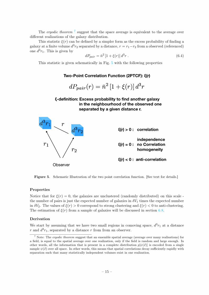
This statistic ξ(r) can be defined by a simpler form as the excess probability of finding agalaxy at a finite volume d3r2 separated by a distance, r = r1−r2 from a observed (referenced)one d3r1. This is given by

dPpair = n2 [1 + ξ(r)] d3r . (6.4)

This statistic is given schematically in Fig. 5 with the following properties

Figure 5. Schematic Illustration of the two point correlation function. [See text for details.]

Properties

Notice that for ξ(r) = 0, the galaxies are unclustered (randomly distributed) on this scale -the number of pairs is just the expected number of galaxies in δV1 times the expected numberin δV2. The values of ξ(r) > 0 correspond to strong clustering and ξ(r) < 0 to anti-clustering.The estimation of ξ(r) from a sample of galaxies will be discussed in section 6.8.

Derivation

We start by assuming that we have two small regions in comoving space, d3r1 at a distancer and d3r1, separated by a distance r from from an observer.

7 Note: The ergodic theorem suggest that an ensemble spatial average (average over many realisations) fora field, is equal to the spatial average over one realization, only if the field is random and large enough. Inother words, all the information that is present in a complete distribution p[ψ(~x)] is encoded from a singlesample ψ(~x) over all space. In other words, this means that spatial correlations decay sufficiently rapidly withseparation such that many statistically independent volumes exist in one realization.

– 15 –

DRAFT

We have that the number of galaxies dN(r1, r2) in the volume d3r2 distant from galaxy1 in the volume d3r1 separated by a distance r is given by:

dN(r1, r2) = n(r1)d3r1n(r1 + r2)d3r2 . (6.5)

we assume now that the number density field has only small perturbations around amean number density n0 = n today. This is written as:

n(r) = n [1 + δ(r)] (6.6)

where δ(r) describes the fluctuations (or overdensities) from the mean n0. Substituting Eq. 6.6to Eq. 6.5, we have that:

dN(r1, r2) = n2 [1 + δ(r1)] d3r1 [1 + δ(r1 + r2)] d3r2 (6.7)

which can be rewritten as:

dN(r1, r2) = n2 [1 + δ(r1)] [1 + δ(r1 + r2)] d3r1d3r2 (6.8)

Assuming that the perturbations are small on average for the whole distribution δ2(r1) 'δ2(r1 + r2) ' 0 we have that :

dN(r1, r2) = n2 [1 + δ(r1)δ(r1 + r2)] d3r1d3r2 (6.9)

By taking the average over the whole volume d3r1, we have that:

dN(r2) :=1

V1

∫V1

d3r1dN(r1, r2) = n2

[1

V1

∫V1

d3r1 +1

V

∫Vd3r1δ(r1)δ(r1 + r2)

]dr2 (6.10)

which can rewritten simplified by removing the subscript for convenience r1 = x, r2 = r andV1 = V2 = V :

dPpair := dN(r) = n2

[1 +

1

V

∫Vd3xδ(x)δ(x+ r)

]d3r (6.11)

Then the two point correlation function is defined as:

ξ(r) :=1

V

∫Vd3xδ(x)δ(x+ r) (6.12)

Therefore, we havedPpair = n2 [1 + ξ(r)] d3r . (6.13)

Therefore it is straight forward to see that the correlation function describes the excess prob-ability of finding a galaxy at a finite volume d3r2 separated by a distance, r from a referencedone d3r1.

6.3 The power spectrum

Another convenient tool to measure the clustering in Fourier space is the power spectrum.This is related to the two point correlation function discussed above. The following Fouriertransform is adopted:

δ(k) =

∫d3rδ(r)eikr , (6.14)

– 16 –

DRAFT

δ(r) =

∫d3r

(2π)3δ(k)e−ikr . (6.15)

The power spectrum is defined via:

P (k1, k2) =1

(2π)3〈δ(k1)δ(k2)〉 , (6.16)

with statistical homogeneity and isotropy giving:

P (k1, k2) = δD(k1 − k2)P (k1) (6.17)

where δD is the Dirac delta function of a 3D field. The correlation function and the powerspectrum are therefore a Fourier pair as:

P (k) =

∫ξ(r)eikrd3r , (6.18)

ξ(k) =

∫P (k)e−ikr

d3r

(2π)3, (6.19)

since they provide the same information. The choice of which to use is therefore somewhatarbitrary, see discussion by Percival [26].

6.4 Fractal Dimension

Nature all around us is full of fractal patterns, be it from amazing snowflakes to romanescobroccoli. Naturally due to the peculiar structure of galaxies around us, there were severalclaims that the universe behaving like a fractal one (Labini et al. [27], Coleman and Pietronero[28]). Therefore we can study the fractality of the galaxy distributions using the fractaldimension, defined as:

D2(r) ≡ d lnN(< r)

d ln r(6.20)

where N(< r) is the count-in-spheres of galaxies. However the information obtained fromthis statistics it is similar to the one of ξ(r) or P (k) but it is an active field of research onhow we can use it to optimize our observations! It has been shown that the universe at smallscales behaves as a fractal, at scales less than 50h−1Mpc and at large scales it reaches astatistically homogeneous behaviour asymptotically[29–31]. For a homogeneous distributionthe counts-in-spheres scale as the volume, N(< r) ∝ r3, while for a fractal distribution theyscale as N(< r) ∝ rD2 where D2 quantifies the fractality of the distribution in study. Forfurther discussion, see [10] and references therein.

6.5 Anisotropic statistics

Although the true universe is expected to be statistically homogeneous and isotropic, theobserved one is not so due to a number of observational effects discussed in section 7. Statis-tically, these effect are symmetric around the line-of-sight. In the distant-observer limit theseeffects possess a reflectional symmetry along the line-of-sight looking outwards or inwards.Thus, to first order, the anisotropies in the over-density field can be written as a function ofµ which is the cosine angle to the line-of-sight. Consequently, we often write the correlation

– 17 –

DRAFT

function ξ(r, µ), the power spectrum P (k, µ) or the Fractal Dimension, D2(r, µ). It is commonto expand these observables in Legendre polynomials Ll(µ) as:

ξ(r, µ) =∑l

ξ(r)Ll(µ) . (6.21)

Only the first thre even Legendre polynomials are important, as shown by Kaiser [32]; L0(µ) =1, L1(µ) = (3µ2 − 1)/2 and L4(µ) = (35µ4 − 30µ2 + 3)/8. In the absence of redshift spacedistortions, discussed in section 7.3, only the "monopole" or the andgle-averaged correlationfunction survives:

ξ0(r) =1

2

∫ 1

−1dµ ξ(r, µ) . (6.22)

In a similar way, one can expand the fractal dimension in terms of the legendre polyno-mials:

D2(r, µ) =∑l

D2(r)Ll(µ) . (6.23)

and study the anisotropic fractality of large scale structures. Another active area of currentresearch[10]. One can potential study these kind of estimators at different type of galaxies,[30,33] or study the cosmological impact of observing a characteristic scale of homogeneity[34, 35].

6.6 Higher order statistics

At early times and on large scales, we expect the over-density field to have Gaussian statistics.This follows from the central limit theorem, which implies that a density distribution is asymp-totically Gaussian in the limit where the density results from the average of many independentprocesses. The over-density field has zero mean by definition so, in this regime, is completelycharacterised by either the correlation function or the power spectrum. Consequently, mea-suring either the correlation function or the power spectrum provides a statistically completedescription of the field. To capture them on small scale structure, we usually resort to higherorder statistics of the matter field. Higher order statistics tell us about the break-down of thelinear regime, showing how the gravitational build-up of structures occurs and allowing testsof General Relativity.

The extension of the 2-pt statistics, the power spectrum and the correlation function,to higher orders is straightforward. From Eq. 6.13 we have:

dPtuple = nn[1 + ξ(n)

]d3r1 . . . d

3r2 (6.24)

The immediate application of n-point statistics is the Bispectrum, B(k1, k2) defined as:

< δ(k1)δ(k2)δ(k3) >= (2π)3B(k1, k2)δD(k1 − k2 − k3) (6.25)

studying the 3rd order statistics, and the Trispectrum, T (k1, k2, k3), defined as:

< δ(k1)δ(k2)δ(k3)δ(k4) >= (2π)3T (k1, k2, k3)δD(k1 − k2 − k3 − k4) (6.26)

studying the 4th order statistics. As an example take a look at [36–39]. We study thesehigher order statistics to obtain information about the non-linear properties of the matterfield which is caused by the small scale complex astrophysical processes, r ∼ 10 h−1Mpc.

– 18 –

DRAFT

6.7 Non-Gaussianity

At very large scales the power spectrum is theoritized to deviate from the Gaussian case. Ithas been shown that primordial non-Gaussianities are generated in the conventional scenarioof inflation[40]. However they are predicted to be very weak. The primordial non-Gaussianproperties[40] of the matter field are modelled in many different ways and can also be observedby different kind of observables. In our case, we are going to focus to the power spectrumobservable and the so called "local" non-Gaussianity. The "local" model is given by:

Φ = φ+ fNL(φ2 − 〈φ2〉) . (6.27)

Here φ denotes the Gaussian random field while Φ denotes the Bardeen’s gauge-invariantpotential, which on sub-Hubble scales reduces to the usual Newtonian peculiar gravitationalpotential, up to a minus sign. On even larger scales this potential is related to the conservedvariable ζ by

ζ =5 + 3w

3 + 3wΦ (6.28)

where w is the equation of state of the dominant component in the universe. The amountof primordial non-Gaussianity is quantified by the non-linearity parameter fNL. Note that,since Φ ' φ ' 10−5 then fNL ∼ 100 which corresponds to relative non-Gaussian correctionsof the order of 10−3. While ζ is constant on large scales, Φ is not. Thus, there are usuallytwo conventions for Eq. 6.27. The large scale structures (LSS) and the cosmic microwavebackground (CMB) one. In the LSS convention, Φ is linearly extrapolated now, z = 0. Inthe CMB convention Φ describes the primordial non Gaussian potential. Therefore, there isan approximate formula that relates the two observables:

fLSSNL =

G(z =∞)

G(z = 0)fCMB

NL ∼ 1.3fCMBNL (6.29)

where G(z) denotes the linear growth suppression factor relative to the Einstein-de Sitteruniverse. It is customary to report valus of fCMB

NL but there is also convient for the large scalestructure community to use fLSS

NL .So far observations have shown that fNL measurements are consistent with 0, and there-

fore no detection of deviations from the Gaussianity of the matter field were observed yet.However, this is another active field of research[41]!

6.8 Estimators for Correlation function and Fractal Dimension

Let’s brefily discuss the estimators of the correlation function and the fractal dimension fromactual galaxy data. For the correlation dimension what we can observe is the counts-in-cells.These are usually denoted as pairs of galaxies in different cells of r on a given galaxy datacatalogue, GG(r). Therefore we can formally define:

• gg(r) =GG(r)

ng(ng − 1)/2, the normalized number of galaxy pairs separated by r,

• rr(r) =RR(r)

nr(nr − 1)/2, the normalized number of random-point pairs separated by r,

• gr(r) =GR(r)

ngnr, the normalized number of galaxy random-point pairs separated by r,

– 19 –

DRAFT

where ng and nr are the total number of galaxies and random points, respectively. A usualestimator of the correlation function is the Peebles-Hauser estimator, ξ(r) = dd(r)/rr(r)− 1,for the two-point correlation function Peebles and Hauser [42]. This estimator is known tobe less efficient than the more sophisticated Landy and Szalay [43] estimator.

ξls(r) =gg(r)− 2gr(r) + rr(r)

rr(r), (6.30)

which has minimal variance on scales where ξ(r) << 1.It has been shown that the optimal weighting of galaxies, for a precise measurement of

the BAO peak, is to assign a weight to each galaxy Reid et al. [44]:

wgal = (wcp + wnoz − 1)× wstar × wsee × wFKP , (6.31)

Here, the close-pair weight, wcp, accounts for the fact that, due to fiber coating, one cannotassign optical fibers on the same plate to two targets closer than 62′′. The wnoz weightaccounts for targets for which the pipeline failed to measure the redshift. The wstar and wseeweights correct for the dependance of the observed galaxy number density with the stellardensity and with seeing, respectively. Finally, we use the FKP weight, wFKP , Feldman et al.[45] in order to reduce the variance of the two-point correlation function estimator. Since wehave introduced the random pairs in our analysis we have no longer access to the counts-in-spheres, but to the normalised counts-in-spheres

N (< r) = Ndata(< r)/Nrandoms(< r) . (6.32)

However, we can directly compute the normalised counts-in-spheres from the correlation func-tion:

N (< r) = 1 +3

r3

∫ r

0ξls(s)s

2ds . (6.33)

It has been shown that this estimator is expected to be the most optimal by Ntelis et al. [30].Applying the previous result to equation Eq. 6.20 our estimator for the fractal correlationdimension is given by:

D2 = 3 +d ln

d ln r

[1 +

3

r3

∫ r

0ξls(s)s

2ds

]. (6.34)

Throughout this document, we drop the hats for sake of simplicity. Estimators of the theo-retical predictions of these observables are publicly available at COSMOlogical Python InitialToolkit (COSMOPIT).

7 Limits on information mining

What can we extract from these observables? What information about the universe is acces-sible to us, directly or indirectly? What are there fundamental limits that underlie to ourknowledge? Generally, the intrinsic limits-to the information we can have access to-are due tothe finite speed of propagation of light. This is an information encoded by Special Relativityand General Relativity. The information that we extract comes from the photons arriving toour devices. This phenomenon gives also rise to the cosmic bias. Finally, an additional com-plications arise from the peculiar motion of the celestial objects on the sky. In this section,we are going to describe the effect of causal diagrams, the cosmic bias and the redshift spacedistortions. This section is based on Leclercq et al. [46] and Ntelis [10].

– 20 –

DRAFT

7.1 Causal diagrams

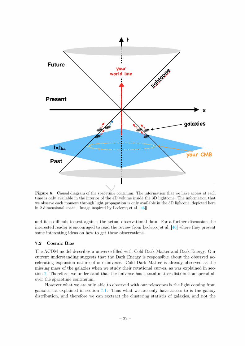
According to special relativity, there is a causal structure of the universe that is relevant forcosmology. In fact, it is only possible to observe part of the universe at a given time. This factlimits the information available for making statistical statements about scales comparable tothe entire observable Universe. Since only a single realization from the ensemble of universes isaccessible to us, statements about the largest scales are subject to uncertainty, usually referredto as cosmic variance. Causal diagrams are a convenient tool to visualize the informationaccessible directly or indirectly. They depict relativistic light cones whose surfaces describethe temporal evolution of light rays in space-time. These diagrams include both a future part(everything that you can possibly influence) and a past part (everything that can possiblyhave influenced you). On causal diagrams, your world line, i.e. your trajectory in space-time, is essentially a straight line orthogonal to the spatial space (the t-axis), for a stationaryobserver. As usual, for graphical convenience, we will suppress the three spatial dimensionand represent the four-dimensional space-time in 2+1 dimensions. In addition, we will usecomoving coordinates to factor out the expansion of the Universe, so that light-rays travel ondiagonal lines. To examine further the causal structure of our universe, we will successivelyconsider three categories: the information we can access now, directly; the information wecould access directly, in a Universe’s lifetime and the information we can access indirectly.

Information accessible directly, now. - Causality allows direct access, now, to:

• the surface of your past light cone (a 3D volume): all the photons that reach you now(e.g. photons from distant galaxies or from the CMB),

• the interior of your past light cone (a 4D volume): all events that could possibly influenceyou via a slower-than-light signal (this includes the gravitational field from massiveobjects or cosmic particles that you receive from space).

Fig. 6 illustrates the 3D lightcone and the information you can have access to directly.Your "CMB circle? (the last scattering sphere in 3D) is the intersection of a plane (3D Volumein reality) − corresponding to the time of last scattering sphere t = tlss, i.e. the time whenthe CMB was emitted − and your past light cone.

Information accesible directely, over time - With the passing of time, progressively wereceive more information through light. If one takes a telescope and gaze the galaxies at afixed time, t = t1, he will obtain information from the 4D lightcone of this particular time.At each moment of his world line there is a 4D lightcone. The more time he observes, themore 4D lightcones he observes and the more information he obtains. Note that for a finiteage of the universe, at any given time, there are regions of the t = 0 3D plane that we havenot yet observed. Take the CMB for instance. The CMB we have access to changes withtime, because the intersection of the 3D plane corresponding to the time of last scatteringsphere t = tlss, and the 3D lightcone changes when we consider a different lightcone. Thismeans that in principle, waiting (for a long time!) allows access to a thick ring in the lastscattering plane, i.e. the CMB map turns into a 3D CMB map.

Information accesible inderectly - If we want information that it is not directly accessibleto us and we do not want to wait there is another option. The naive way is to proceedalso indirectely. Knowing the laws of physics we can infer the behaviour of the universe indifferent regions of the spacetime continuum. Essentially, we can evolve observations forwardand backward in the 4D volume and predict events in the interior (evolution backwards) orexterior (evolution forward) of our 3D lightcone. However such studies are model dependent

– 21 –

DRAFT

Figure 6. Causal diagram of the spacetime continum. The information that we have access at eachtime is only available in the interior of the 4D volume inside the 3D lightcone. The information thatwe observe each moment through light propagation is only available in the 3D lighcone, depicted herein 2 dimensional space. [Image inspired by Leclercq et al. [46]]

and it is difficult to test against the actual observational data. For a further discussion theinterested reader is encouraged to read the review from Leclercq et al. [46] where they presentsome interesting ideas on how to get those observations.

7.2 Cosmic Bias

The ΛCDM model describes a universe filled with Cold Dark Matter and Dark Energy. Ourcurrent understanding suggests that the Dark Energy is responsible about the observed ac-celerating expansion nature of our universe. Cold Dark Matter is already observed as themissing mass of the galaxies when we study their rotational curves, as was explained in sec-tion 2. Therefore, we understand that the universe has a total matter distribution spread allover the spacetime continuum.

However what we are only able to observed with our telescopes is the light coming fromgalaxies, as explained in section 7.1. Thus what we are only have access to is the galaxydistribution, and therefore we can exctract the clustering statistis of galaxies, and not the

– 22 –

DRAFT

total matter of the universe. It turns out, when we compare the clustering statistic of ourtracers and compare it with the theoretical prediction of the clustering statistic of the totalmatter of the universe, we end up having a biased relation between the two. The commonstatistic that defines this biased relation is usually given through the two point correlationfunction:

ξtracer(r) = b2ξmatter(r) (7.1)

where ξtracer(r) is the two point correlation function of our tracer, usually the galaxy dis-tribution, ξmatter(r) is the two point correlation function of the total matter of the universeand b is the cosmic bias or bias. There is an active field of research of exploring models ofdifferent kinds of biases, such as the local bias, or scale dependent biases[41].

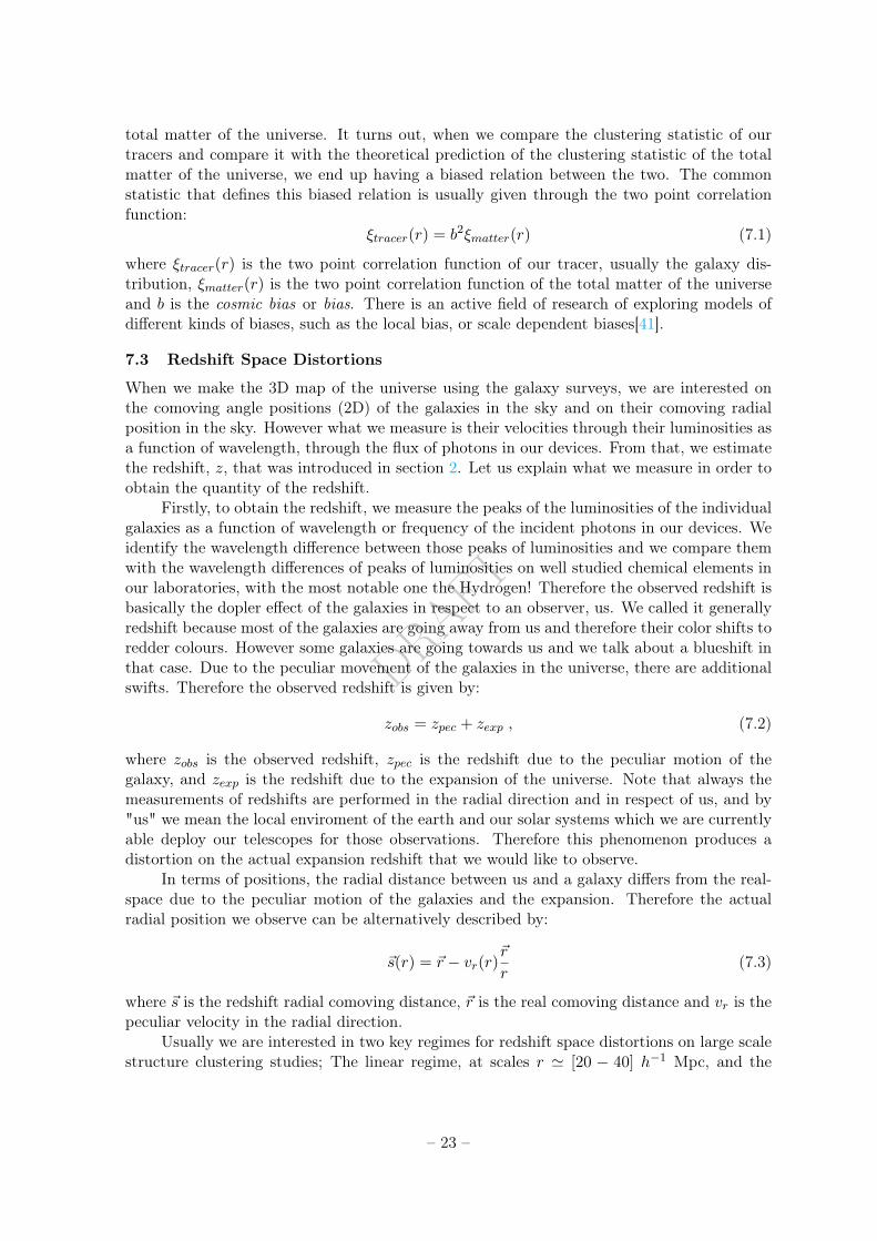
7.3 Redshift Space Distortions

When we make the 3D map of the universe using the galaxy surveys, we are interested onthe comoving angle positions (2D) of the galaxies in the sky and on their comoving radialposition in the sky. However what we measure is their velocities through their luminosities asa function of wavelength, through the flux of photons in our devices. From that, we estimatethe redshift, z, that was introduced in section 2. Let us explain what we measure in order toobtain the quantity of the redshift.

Firstly, to obtain the redshift, we measure the peaks of the luminosities of the individualgalaxies as a function of wavelength or frequency of the incident photons in our devices. Weidentify the wavelength difference between those peaks of luminosities and we compare themwith the wavelength differences of peaks of luminosities on well studied chemical elements inour laboratories, with the most notable one the Hydrogen! Therefore the observed redshift isbasically the dopler effect of the galaxies in respect to an observer, us. We called it generallyredshift because most of the galaxies are going away from us and therefore their color shifts toredder colours. However some galaxies are going towards us and we talk about a blueshift inthat case. Due to the peculiar movement of the galaxies in the universe, there are additionalswifts. Therefore the observed redshift is given by:

zobs = zpec + zexp , (7.2)

where zobs is the observed redshift, zpec is the redshift due to the peculiar motion of thegalaxy, and zexp is the redshift due to the expansion of the universe. Note that always themeasurements of redshifts are performed in the radial direction and in respect of us, and by"us" we mean the local enviroment of the earth and our solar systems which we are currentlyable deploy our telescopes for those observations. Therefore this phenomenon produces adistortion on the actual expansion redshift that we would like to observe.

In terms of positions, the radial distance between us and a galaxy differs from the real-space due to the peculiar motion of the galaxies and the expansion. Therefore the actualradial position we observe can be alternatively described by:

~s(r) = ~r − vr(r)~r

r(7.3)

where ~s is the redshift radial comoving distance, ~r is the real comoving distance and vr is thepeculiar velocity in the radial direction.

Usually we are interested in two key regimes for redshift space distortions on large scalestructure clustering studies; The linear regime, at scales r ' [20 − 40] h−1 Mpc, and the

– 23 –

DRAFT

non-linear regime, r . 10 h−1 Mpc. The linear regime is described by the Kaiser model[32],while for the non-linear regime there are several descriptions and it is an active research fieldin cosmology due to complex astrophysical phenomena.

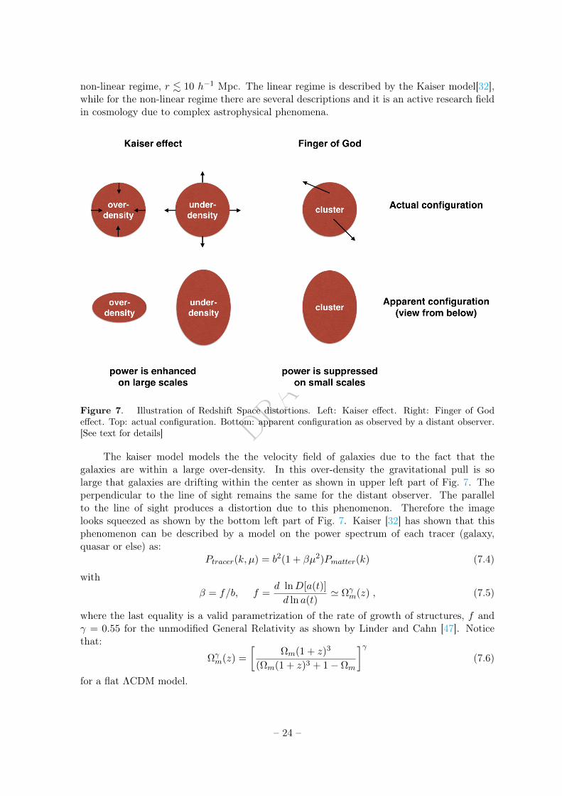
Figure 7. Illustration of Redshift Space distortions. Left: Kaiser effect. Right: Finger of Godeffect. Top: actual configuration. Bottom: apparent configuration as observed by a distant observer.[See text for details]

The kaiser model models the the velocity field of galaxies due to the fact that thegalaxies are within a large over-density. In this over-density the gravitational pull is solarge that galaxies are drifting within the center as shown in upper left part of Fig. 7. Theperpendicular to the line of sight remains the same for the distant observer. The parallelto the line of sight produces a distortion due to this phenomenon. Therefore the imagelooks squeezed as shown by the bottom left part of Fig. 7. Kaiser [32] has shown that thisphenomenon can be described by a model on the power spectrum of each tracer (galaxy,quasar or else) as:

Ptracer(k, µ) = b2(1 + βµ2)Pmatter(k) (7.4)

withβ = f/b, f =

d lnD[a(t)]

d ln a(t)' Ωγ

m(z) , (7.5)

where the last equality is a valid parametrization of the rate of growth of structures, f andγ = 0.55 for the unmodified General Relativity as shown by Linder and Cahn [47]. Noticethat:

Ωγm(z) =

[Ωm(1 + z)3

(Ωm(1 + z)3 + 1− Ωm

]γ(7.6)

for a flat ΛCDM model.

– 24 –

DRAFT

The non-linear regime is described empirically by the "Finger of God" effect whichmodels by the dispersion of the peculiar velocity field of the galaxies at the cluster level, fewkpc. In the litarature there are several models [48], so someone can take an compare thesemodel according to their data. The Finger of God effect supresses the power spectrum atsmall scales, i.e. at large k modes due to the peculiar motions of the galaxies. Therefore theDamping models are summarised by:

DG(k, µ;σp, H0) = exp

[−(kµσpH0

)2],Gaussian (7.7)

and theDL(k, µ;σp, H0) =

1

1 + 12

(kµσpH0

)2 ,Lorentzian (7.8)

These dumbs the theoretical model at smaller scales r < 10 h−1Mpc according to:

Ptracer,final(k, µ; b, σp;H0) = DX(k, µ;σp, H0)Ptracer(k, µ) (7.9)

where DX is either the Lorentzian model or the Gaussian model for damping.

8 Large scale structure surveys, status

Large scale structure surveys are usually devided into two big categories. The ones whichfocus on studying the primordial universe and the ones that focus on studying the late timeuniverse. Often we use the their results to extract the physical information that explains bothregimes of observations. The model that we are trying to describes is the ΛCDM model thatexplains the universe as a whole. The primordial universe observations are focus on studyingthe primordial temperature fluctuations. They study the Cosmic Microwave Background andthere are several interesting physics going on.

Here we are going to the second part of observations, the ones that study the late timeuniverse. At that time there are several models about the structure formation, content ofthe universe as well as alternative models of Gravity and many more. These observations areachieved by the so called, "large scale structure surveys". To perform such observations, weuse telescopes that basically map the two dimensional position on the sky of several objects, aslong as the luminosities of those objects. From the luminocities we can deduce velocities andradial distances and we can do a lot of interesting science with them! The basic observablethat we use is the three Dimensional comoving density field and many of the reconstructionsof that we tryied to summarise in section 6. Let’s see what are the main instruments thatare useful to extract the above information. The main characteristic that we are interested incosmology, and large scale structure physics, is the redshift of each object that we describedin section 2, therefore these surveys are called Redshift Surveys or Galaxy Surveys, since themain targets are galaxies.

The Redshift Surveys are usually devided into ground based and satellites. However,the satellite redshift surveys is a relative new theme of instruments that we are currentlyinvestigating, with the ongoing mission named, "Euclid Mission". The advantage of groundbased observations is that we can easily modify the instrument, as well as the ongoing processof constructing it and testing it against observations is faster. However this allow for a veryvast spectrum of different kind of instruments. However, they are subtle to atmospheric noise.

– 25 –

DRAFT

Therefore, for the first time, Euclid Mission is prepered to study the large scale structure in thelate universe from space. The other important devision of instruments is that of Spectroscopyand Photometry that we will describe in the next two paragraphs.

In Photometry, instruments are build in such a way to take fast images of the sky.Photons transverse coloured filters and map the spectrum (flux as a function of wavelength)of the observed targets. The advantages are that they can perform fast imaging, with a goodSignal to noise ratio (SNR), since one simple detector pipeline is used. Therefore they areable to perform massive data collection. However, their disadvantage is that they have a verysmall resolution on the wavelength.

In Spectroscopic instruments the photons transverse a sequences of dispersive materialsso that we can map more precisely and accurately the spectrum of the targets. The advan-tages are that they perform an exquisite δλ resolution. However, they have low SNR, sincemultiple detector elements are required of the photon pipeline. Furthermore, they performslow imaging, since they require high exposure time. However, several robotic mechanismsare under development to ameliorate their speed and SNR.

Currently, the Sloan Digital Sky Survey (SDSS)[49] is observing the redshift region from0 ≤ z ≤ 3.5 targeting millions of galaxies and thousands of QSO with their correspondingLyman-α forests. The main project is dedicated to cosmology and large scale structures.It has the name the extended Baryon Oscillation Spectroscopy Survey (eBOSS). The DarkEnergy Spectroscopy Instrument (DESI)[50] is a dedicated project to study the large scalestructure from the ground. We expect the first light in 2019. In 2019, we expect also thefirst light from the Large Synoptic Survey Telescope (LSST)[51] which is a sophisticate basedphotometric instrument with the a camera with the largest field of view for redshift surveys.Finally the Euclid Mission[52], is expected to give the first light in 2022, and is going to mapthe 3D comoving galaxy distribution in redshift 0.9 < z < 1.8 and study the dark universemainly from galaxy clustering and weak lensing. Currently, at CPPM[53], researcher aredeveloping some characterisation of its NISP instrument[54]. All those instrument, targetsome overlapping regions to calibrate on one an another and explore as much as possible thevast universe!

9 Statistical inference

Information theory is a framework where the way of making decisions from a collection ofdata is studied 8. One of the main things that we are interested from this framework isthe statistical analysis or statistical inference. When discussing statistical data analysis, twodifferent points of view are traditionally reviewed and opposed: the frequentist (see e.g. [55])and the Bayesian approaches. It is commonly known that arguments for or against eachof them are generally on the level of a philosophical or ideological position, at least amongcosmologists today, 2018. Before criticizing this controversy, somewhat dated to the 20thcentury, and stating that more recent scientific work suppresses the need to appeal to such

8Fun Fact: In the framework of information theory the quote of Sokratis, "one think I know, that I knownnothing", interpretes the equation EX [I(X)] = lnn, where I(x) is the self-information, which is the entropycontribution of an individual message, and EX is the expected value for n messages. Proof : Let X be the setof all messages x1, . . . xn that an X random variable could be, and p(x) is the probability of some x ∈ X ,then the entoropy, H, of X is defined as EX [I(x)] = H(X) = −

∑x∈X p(x) ln p(x). A property of entropy is

that it is maximized when all the messages in the message space are equiprobable, p(x) = 1/n, i.e. the mostunpredictable, in which case EX [I(x)] = lnn.

– 26 –

DRAFT

arguments, we report the most common statements encountered. This section is based onLeclercq [56].

9.1 Bayesian vs Frequentist

Frequentist and Bayesian statistics differ in the epistemological interpretation of probabilityand their consequences for hypotheses testing and models comparison. Firstly, the methodsdiffer on the understanding of the concept of the probability P (A) of an event A. As afrequentist, one defines the probability P (A) as the relative frequency with which the eventA occurs in repeated experiments, i.e. the number of times the event occurs over the totalnumber of trials, in the limit of a infinite series of equiprobable repetitions. This probability(definition) has several caveats. Besides being useless in real life (as it assumes an infiniterepetition of experiments with nominally identical test conditions, requirement that is nevermet in most practical cases), it cannot handle unrepeatable situations, which have a particularimportance in cosmology, as we have exactly one sample of the Universe. More importantly,this definition is surprisingly circular, in the sense that it assumes that repeated trials areequiprobable, despite that it is the very notion of probability that is being defined in the firstplace.

On the other hand, in Bayesian statistics, the probability P (A) represents the degreeof belief that any reasonable person (or machine) shall attribute to the occurrence of eventA under consideration of all available information. This definition implies that in Bayesiantheory, probabilities are used to quantify uncertainties independently of their origin, andtherefore applies to any event. In other words, probabilities represent a state of knowledge inpresence of partial information. This is the intuitive concept of probability as introduced byseveral authors such as Laplace, Bayes, Bernoulli, Metropolis, Jeffreys, etc.[57].

Translated to the measurement of a parameter in an experiment, the aforementioneddefinitions of probabilities yield differences in the questions addressed by frequentist andBayesian statistical analyses. In the frequentist point of view, statements are structured as:"the measured value x occurs with probability P (x) if the measured quantity X has the truevalue XT ". This means that the only questions that can be answered are of the form: "giventhe true value XT of the measured quantity X, what is the probability distribution of themeasured values x?". It also implies that statistical analyses are about building estimators,X, of the truth, XT .

In contrast, Bayesian statistics allows statements of the form: "given the measured valuex, the measured quantity X has the true value XT with probability P". Therefore, one can alsoanswer the question: "given the observed measured value x, what is the probability that the truevalue of X is XT ?", which arguably is the only natural thing to demand from data analysis.For this reason, Bayesian statistics offers a principled approach to the question underlyingevery measurement problem, of how to infer the true value of the measured quantity givenall available information, including observations. In summary, in the context of parameterdetermination, the fundamental difference between the two approaches is that frequentiststatistics assumes the measurement to be uncertain and the measured quantity known, whileBayesian statistics assumes the observation to be known and the measured quantity uncertain.Similar considerations can be formulated regarding the problems of hypothesis testing andmodel comparison.

– 27 –

DRAFT

9.2 Bayesian Framework

The "plausible reasoning" can be formulated mathematically by introducing the concept ofconditional probability P (A|B), which describes the probability that the event A will occurgiven the information B which is given on the right side of the vertical conditioning bar "|".To conditional probabilities applies the following famous identity, which allows to go fromforward modelling to the inverse problem, by noting that if one knows how x arises from y,then one can use x to constrain y:

P (y|x)P (x) = P (x|y)P (y) = P (x, y) (9.1)

This observation forms the basis of Bayesian statistics.Therefore, Bayesian analysis is a general method for updating the probability estimate

for a theory in light of new data. It is based on Bayes’ theorem,

P (θ|d) =P (d|θ)P (θ)

P (d), (9.2)

where θ represents the set of the parameter space of a particular model of a particular theoryand d represents the data or evidence (before the data are known). The above formula isinterpreted as follows:

• P (d|θ) is the probability of the data before they are known, given the theory. It isusually called the likelihood.

• P (θ) is the probability of theory in the absence of data. It is called the prior probabilitydistribution function or simply the prior.

• P (θ|d) is the probability of the theory, after the data are known. It is called the posteriorprobability distribution function or simply the posterior.

• P (d) is the probability of the data before they are known, without any assumptionabout the theory. It is called the evidence.

One can think that the probability distribution function (pdf) for an uncertain parametercan be thought as a "belief distribution function", quantifying the degree of truth that oneattributes to the possible values for some parameter. Certainty can be represented by a Diracdistribution, e.g. if the data determine the parameters completely.

In summary, the inputs of a Bayesian analysis are two:

• the data: include for example, the galaxy angle position in the sky, galaxy redshift,photometric redshift pdfs, the temperature in pixels of a CMB map, etc. Details of thesurvey specifications have also to be accounted for at this point: noise, mask, surveygeometry, selection effects, biases, etc.

• the prior: it includes modelling assumptions, both theoretical and experimental. Spec-ifying a prior is a systematic way of quantifying what one assumes true about a theorybefore looking at the data.

While the output of a Bayesian analysis is the posterior density function. The prior choice isa key ingredient of Bayesian statistics. It is sometimes considered problematic, since there isno unique prescription for selecting the prior. Here we can argue that prior specification is

– 28 –

DRAFT

not a limitation of Bayesian statistics and does not undermine objectivity. One can simplydetermine the prior knowledge that he consider and compare with studies that have useddifferent prior. The discussion of selecting the appropriate prior is beyond the scope of thesenotes and the reader is redirected to Leclercq [56].

9.3 Statistical indeference problem

Data analysis problems can be typically classified as: parameter inference, model comparison,hypothesis testing. For example, cosmological questions of these three types, related to thelarge-scale structure, would be:

• What is the value of the dark energy density ratio, ΩΛ?

• Is structure formation driven by general relativity or by modified gravity?

• Are large-scale structure observations consistent with the hypothesis of an inflationaryscenario?

In this section, we describe the methodology for questions of the first two types. Hypothesistesting, i.e. inference within an uncertain model, in the absence of an explicit alternative,can be treated in a similar manner.

9.4 First level inference: parameter estimation

The general problem of parameter estimation can be stated as follows. Given a physicalmodel M , a set of hypotheses is specified in the form of a vector of parameters, θ. Togetherwith the model, priors for each parameter must be specified: P (θ|M). The next step is toconstruct the likelihood function for the measurement, with a probabilistic, generative modelof the data: P (d|θ,M). The likelihood reflects how the data are obtained: for example, ameasurement with Gaussian noise will be represented by a normal distribution.

Once the prior is specified and the data is incorporated in the likelihood function, oneimmediately obtains the posterior distribution for the model parameters, integrating all theinformation known to date, by using Bayes’ theorem eq. 9.2:

P (θ|d,M) =P (d|θ,M)P (θ|M)

P (d)(9.3)

Note that the normalizing constant, namely Bayesian evidence is defined as:

P (d) =

∫M

∫θP (d|θ,M) =

∫M1

· · ·∫Mn

∫~θ1

· · ·∫~θn

p(d|M1(~θ1) . . .Mn( ~θn)) (9.4)

where∫x f(x) =

∫X f(x)dx implies the usual Remannian integration. The Bayesian evidence

is irrelevant for parameter inference (but fundamental for model comparison, see section 9.7).Usually, the set of parameters θ can be divided in some physically interesting quantities φ anda set of nuisance parameters n. The posterior obtained by eq. 9.3 is the joint posterior forθ = (φ, n). The marginal posterior for the parameters of interest is written as (marginalizingover the nuisance parameters):

P (φ|d,M) ∝∫P (d|φ, n,M)P (φ, n|M)dn . (9.5)

– 29 –

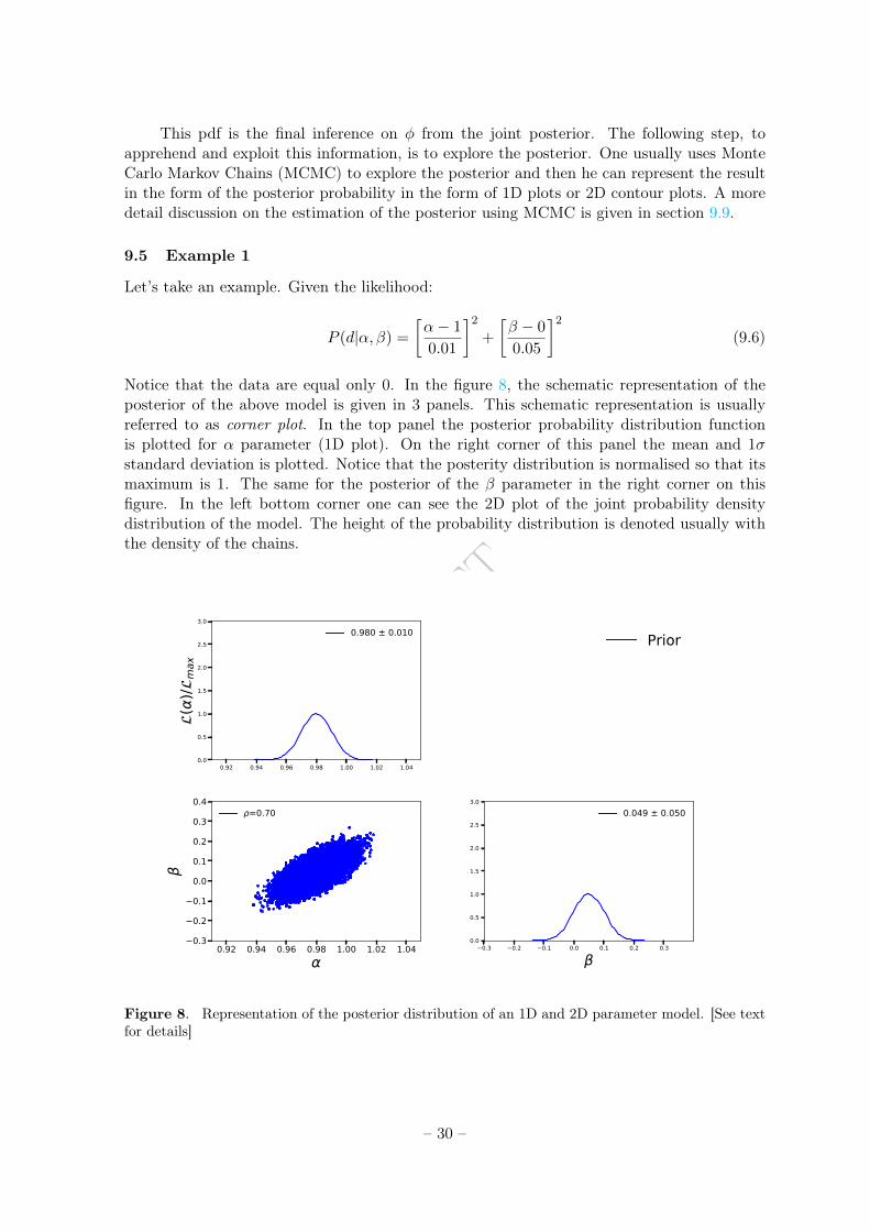
DRAFT

This pdf is the final inference on φ from the joint posterior. The following step, toapprehend and exploit this information, is to explore the posterior. One usually uses MonteCarlo Markov Chains (MCMC) to explore the posterior and then he can represent the resultin the form of the posterior probability in the form of 1D plots or 2D contour plots. A moredetail discussion on the estimation of the posterior using MCMC is given in section 9.9.

9.5 Example 1

Let’s take an example. Given the likelihood:

P (d|α, β) =

[α− 1

0.01

]2

+

[β − 0

0.05

]2

(9.6)

Notice that the data are equal only 0. In the figure 8, the schematic representation of theposterior of the above model is given in 3 panels. This schematic representation is usuallyreferred to as corner plot. In the top panel the posterior probability distribution functionis plotted for α parameter (1D plot). On the right corner of this panel the mean and 1σstandard deviation is plotted. Notice that the posterity distribution is normalised so that itsmaximum is 1. The same for the posterior of the β parameter in the right corner on thisfigure. In the left bottom corner one can see the 2D plot of the joint probability densitydistribution of the model. The height of the probability distribution is denoted usually withthe density of the chains.

0.92 0.94 0.96 0.98 1.00 1.02 1.040.0

0.5

1.0

1.5

2.0

2.5

3.0

()/

max

0.980 ± 0.010

0.92 0.94 0.96 0.98 1.00 1.02 1.040.3

0.2

0.1

0.0

0.1

0.2

0.3

0.4=0.70

0.3 0.2 0.1 0.0 0.1 0.2 0.30.0

0.5

1.0

1.5

2.0

2.5

3.00.049 ± 0.050

Prior

Figure 8. Representation of the posterior distribution of an 1D and 2D parameter model. [See textfor details]

– 30 –

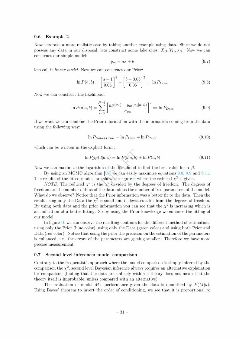
DRAFT

9.6 Example 2

Now lets take a more realistic case by taking another example using data. Since we do notpossess any data in our disposal, lets construct some fake ones, XD, YD, σD. Now we canconstruct our simple model:

ym = ax+ b (9.7)

lets call it linear model. Now we can construct our Prior:

lnP (a, b) =

[a− 1

0.05

]2

+

[b− 0.05

0.05

]2

:= lnPPrior (9.8)

Now we can construct the likelihood:

lnP (d|a, b) =

N−1∑i=0

[yD(xi)− ym(xi|a, b)

σyD

]2

:= lnPData (9.9)

If we want we can combine the Prior information with the information coming from the datausing the following way:

lnPData+Prior = lnPData + lnPPrior (9.10)

which can be written in the explicit form :

lnPDP (d|a, b) = lnP (d|a, b) + lnP (a, b) (9.11)

Now we can maximize the logarithm of the likelihood to find the best value for α, β.By using an MCMC algorithm [58] we can easily maximize equations 9.8, 9.9 and 9.11.

The results of the fitted models are shown in figure 9 where the reduced χ2 is given.NOTE : The reduced χ2 is the χ2 devided by the degrees of freedom. The degrees of

freedom are the number of bins of the data minus the number of free parameters of the model.What do we observe? Notice that the Prior information was a better fit to the data. Then theresult using only the Data the χ2 is small and it deviates a lot from the degrees of freedom.By using both data and the prior information you can see that the χ2 is increasing which isan indication of a better fitting. So by using the Prior knowledge we enhance the fitting ofour model.

In figure 10 we can observe the resulting contours for the different method of estimationsusing only the Prior (blue color), using only the Data (green color) and using both Prior andData (red color). Notice that using the prior the precision on the estimation of the parametersis enhanced, i.e. the errors of the parameters are getting smaller. Therefore we have moreprecise measurement.

9.7 Second level inference: model comparison

Contrary to the frequentist’s approach where the model comparison is simply inferred by thecomparison the χ2, second level Bayesian inference always requires an alternative explanationfor comparison (finding that the data are unlikely within a theory does not mean that thetheory itself is improbable, unless compared with an alternative).

The evaluation of model M ’s performance given the data is quantified by P (M |d).Using Bayes’ theorem to invert the order of conditioning, we see that it is proportional to

– 31 –

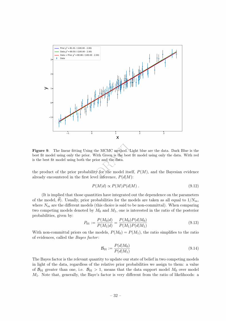
DRAFT1 0 1 2 3

x

1

0

1

2

3

yPrior 2 = 81.01 / (100.00 - 2.00) Data 2 = 80.50 / (100.00 - 2.00) Data + Prior 2 = 80.86 / (100.00 - 2.00) Data

Figure 9. The linear fitting Using the MCMC method. Light blue are the data. Dark Blue is thebest fit model using only the prior. With Green is the best fit model using only the data. With redis the best fit model using both the prior and the data.

the product of the prior probability for the model itself, P (M), and the Bayesian evidencealready encountered in the first level inference, P (d|M):

P (M |d) ∝ P (M)P (d|M) . (9.12)

(It is implied that those quantities have integrated out the dependence on the parametersof the model, ~θ). Usually, prior probabilities for the models are taken as all equal to 1/Nm,where Nm are the different models (this choice is said to be non-committal). When comparingtwo competing models denoted by M0 and M1, one is interested in the ratio of the posteriorprobabilities, given by:

P01 :=P (M0|d)

P (M1|d)=P (M0)P (d|M0)

P (M1)P (d|M1)(9.13)

With non-committal priors on the models, P (M0) = P (M1), the ratio simplifies to the ratioof evidences, called the Bayes factor :

B01 :=P (d|M0)

P (d|M1)(9.14)

The Bayes factor is the relevant quantity to update our state of belief in two competing modelsin light of the data, regardless of the relative prior probabilities we assign to them: a valueof B01 greater than one, i.e. B01 > 1, means that the data support model M0 over modelM1. Note that, generally, the Baye’s factor is very different from the ratio of likelihoods: a

– 32 –

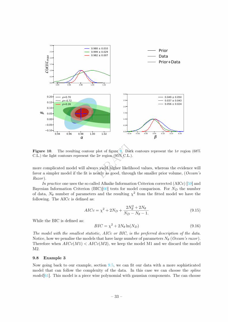
DRAFT

0.94 0.96 0.98 1.00 1.020.0

0.5

1.0

1.5

2.0

2.5

3.0(

)/m

ax0.980 ± 0.0100.999 ± 0.0290.982 ± 0.007

0.94 0.96 0.98 1.00 1.020.10

0.05

0.00

0.05

0.10

0.15

0.20 =0.70=-0.72=0.26

0.10 0.05 0.00 0.05 0.10 0.15 0.200.0

0.5

1.0

1.5

2.0

2.5

3.00.049 ± 0.0500.037 ± 0.0430.056 ± 0.024

PriorDataPrior+Data

Figure 10. The resulting contour plot of figure 9. Dark contours represent the 1σ region (68%C.L.) the light contours represent the 2σ region (95% C.L.).

more complicated model will always yield higher likelihood values, whereas the evidence willfavor a simpler model if the fit is nearly as good, through the smaller prior volume, (Occam’sRazor).

In practice one uses the so called Alkaike Information Criterion corrected (AICc) [59] andBayesian Information Criterion (BIC)[60] tests for model comparison. For ND the numberof data, Nθ number of parameters and the resulting χ2 from the fitted model we have thefollowing. The AICc is defined as:

AICc = χ2 + 2ND +2N2

θ + 2Nθ

ND −Nθ − 1.(9.15)

While the BIC is defined as:BIC = χ2 + 2Nθ ln(ND) (9.16)

The model with the smallest statistic, AICc or BIC, is the preferred description of the data.Notice, how we penalise the models that have large number of parametersNθ (Occam’s razor).Therefore when AICc(M1) < AICc(M2), we keep the model M1 and we discard the modelM2.

9.8 Example 3

Now going back to our example, section 9.5, we can fit our data with a more sophisticatedmodel that can follow the complexity of the data. In this case we can choose the splinemodel [61]. This model is a piece wise polynomial with gaussian components. The can choose

– 33 –

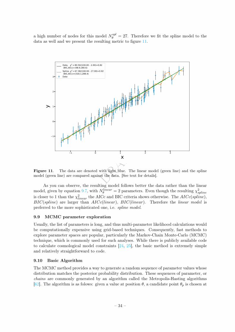
DRAFT

a high number of nodes for this model N splθ = 27. Therefore we fit the spline model to the

data as well and we present the resulting metric to figure 11.

1 0 1 2 3

x

1

0

1

2

3

y

Data, 2 = 80.50/(100.00 - 2.00)=0.82 (BIC,AICc)=(98.9,280.6)Spline, 2 = 67.38/(100.00 - 27.00)=0.92 (BIC,AICc)=(316.1,288.4)Data

Figure 11. The data are denoted with light blue. The linear model (green line) and the splinemodel (green line) are compared against the data. [See text for details].

As you can observe, the resulting model follows better the data rather than the linearmodel, given by equation 9.7, with N linear

θ = 2 parameters. Even though the resulting χ2spline

is closer to 1 than the χ2linear the AICc and BIC criteria shows otherwise. The AICc(spline),

BIC(spline) are larger than AICc(linear), BIC(linear). Therefore the linear model ispreferred to the more sophisticated one, i.e. spline model.

9.9 MCMC parameter exploration

Usually, the list of parameters is long, and thus multi-parameter likelihood calculations wouldbe computationally expensive using grid-based techniques. Consequently, fast methods toexplore parameter spaces are popular, particularly the Markov-Chain Monte-Carlo (MCMC)technique, which is commonly used for such analyses. While there is publicly available codeto calculate cosmological model constraints [24, 25], the basic method is extremely simpleand relatively straightforward to code.

9.10 Basic Algorithm

The MCMC method provides a way to generate a random sequence of parameter values whosedistribution matches the posterior probability distribution. These sequences of parameter, orchains are commonly generated by an algorithm called the Metropolis-Hasting algorithms[62]. The algorithm is as folows: given a value at position θ, a candidate point θp is chosen at

– 34 –

DRAFT

random from a proposal distribution f(θp|θ) - usually by means of a random number generatortuned to this proposal distribution. Then the algorithm has to decide if it will move to thecandidate point. This transition is accepted if the new position has a higher likelihood. If thenew position θp is less likely than θ, then we must draw another random variable, this timewith uniform density between 0 and 1. The θp is accepted, and the chain moves to point θp,if the random variable is less than the ratio of the likelihood of θp and the likelihood of θ.Otherwise the chain "stays" at θ, giving this point extra weight within the sequence. In thelimit of an infinite number of steps, the chains will reach a converged distribution where thedistribution of chain links are representative of the hyper-surface of the likelihood, given anysymmetric proposal distribution f(θp|θ) = f(θ|θp).

It is common to implement dynamic optimisation of the sampling of the likelihoodsurface[63], performed in a period of burn-in at the start of the process. The convergenceis always an issue. How do we know when we have sufficiently long chains that we haveadequately sampled the posterior probability. A number of tests are available [64]. In thenext section 9.11, we describe a test that allows to find the convergence of an MCMC byobtaining the results from different chains started at widely separated locations in parameterspace.

9.11 Tests of MCMC convergence

In order to see if an MCMC parameter estimation algorithm has been converged one usuallyuses several methods. These methods can been classified to the "visual" inspection andthe calculation of different statistics. Visual inspection includes that the walkes of an MCMCoscillate around a common, mean value. The different statistics that are used are the Gelman-Rubin Test [64], the Heidelberger-Welch test[65], the Goodman-Weare test [66]. Here, we aregoing to describe the Gelman-Rubyn test. For an overview of the rest of the tests, see of theAppendix 6.B of [67].

The statistic[64] which is called the Gelman-Rubyn statistic is denoted usually as R.How one computes that? One need to follow the forthcoming steps:

• Draw m independent MCMC realisation of a set parameters pi of a model after n stepsof each chain.

• The new parameters now can be denoted as θij where i = [0, ..., n] and j = [0, ...,m]

• Then computes the quantities the R(θ) for each parameter, θ, as follows:

The mean θj and standard deviation σj of each parameter, for each chain, j:

θj =1

n

n∑i=1

θij , ;σ2j =

1

n− 1

n∑i=1

(θij − θj)2 (9.17)

Then one computes the derived quantities: The mean of the mean

¯θ =1

m

m∑j=1

θj (9.18)

The mean of the variances:

W =1

m

m∑j=1

σ2j (9.19)

– 35 –

DRAFT

The deviations of the mean of the chains from the mean of the of the means:

B =n

m− n

m∑j=1

(θj − ¯θ)2 (9.20)

Then the quantity:V (θ) = (1− 1/n)W +B/n (9.21)

Finally the Gelman-Rubyn statistic is given by:

R(θ) =

√V (θ)

W(9.22)

Compute this statistic with starting from a different iteration of the chains. The Rule ofthumb of convergence is R− 1 < 0.03 or for more demanding results R− 1 < 0.01.

10 Summary & Conclusion

We presented the basic concepts of physics on large scale structures. We gave a brief overviewon the thermal history of our universe. We describe the theoretical framework, behind themagnificent scenery of the current observations, known as the standard ΛCDM model. Wedescribed the necessary tools for observations by introducing the statistical observables cur-rently investigated. We discussed the current and future large scale structure surveys. Finally,we gave an overview on the statistical elements needed to study large scale structures, witha focus on Bayesian Analysis.

The conclusions we draw is that the main interests of modern Cosmology are: to explainthe universe as a whole. There are different ways of handling the data, different kind ofobservables. There are many available competitive scenarios about the universe and there area lot more to explore!

Physics, mathematics, statistics and informatics are valuable skills! Believe it or not,keep on searching! ;-)

Acknowledgements

PN would like to thank Mikhail Stolpovskiy, Ranajoy Banerji, Cyrille Doux, Jean-ChristopheHamilton, James Rich, Andre Tilquin Adam Hawken for fruitful and endless discussions onthese subjects. PN would like to thank the organisers of L’école d’éte France Excellence 2018for such a pleasant environment that created for this event. PN is supported by a CNES PostDoctoral fellowship.

Appendix: Useful Mathematics

A symmetric tensor, T , of dimension, d, and of rank r, usually denoted as Tα1...αr has inde-pendent components according to:(

d+ r − 1r

)=

(d+ r − 1)!

r!(d− 1)!(10.1)

– 36 –

DRAFT

For example, a symmetric tensor, T , of dimension, d, and rank 3, denoted as Tαβγ hasindependent components: (

d+ 3− 13

)=

(d+ 3− 1)!

3!(d− 1)!(10.2)

Now, if it leaves in 3 dimensions, it will have (3+3−1)!3!(3−1)! = 5∗4∗3!

3!2! = 10 components. A commoncase is a symmetric tensor with no trace. In this case the number of indepedent componentsare: (

d+ r − 1r

)−(d+ r − 3r − 2

)(10.3)

Appendix: Cosmography

In order to estimate the power spectrum, the correlation function or any other 3Dimensionalobservable from real data we need to convert Pseudo Equatorial Coordinate into cartesiancoordinates. The pseudo equatorial coordinates of each object in the sky are comprisingof the redshift, z, the Declination, DEC, and Right Ascesion, RA. In order to transformthis information to comoving coordinates we need to translate the redshift information intocomoving radial distance, dC(z), where H(z) is the local hubble expansion rate at redshift, z.

The hubble expansion rate is defined as:

H(z) = H0

√(Ωcdm + Ωb)(1 + z)3 + Ωr(1 + z)4 + Ωk(1 + z)2 + ΩΛ(1 + z)3(1+w) , (10.4)

where Ωx with x = [cdm, b, r,Λ] are the density ratios of the components of the universe, Ωk

describes its curvature and w is the parametrization of the equation of state. For more detailssee[10]. Useful equations below:

Hubble distance:

dH =c

H0' 3× 108 m/s

7× 104 m/s/Mpc' 5Gpc (10.5)

Hubble Volume:VH = d3

H ' 2Gpc3 (10.6)

Comoving Distance:

dC(z) = dH

∫ z

0

dz′

E(z′)(10.7)

where E(z; ~Ω) = H(z)/H0 and H(z) is given by Eq. 10.4.Transverse Comoving Distance(Motion)

dM (z) =

dH√Ωk

sinh(√

ΩkdC(z)dH

), Ωk > 0

dC(z) , Ωk = 0dH√Ωk

sin(√

ΩkdC(z)dH

), Ωk < 0

Angular Diameter Distance dA(z) = s(z)

θ =sizeobject(z)

(Angular apperture of object) :

dA(z) =dM (z)

1 + z(10.8)

– 37 –

DRAFT

Luminocity Distance:dL(z) = (1 + z)dM (z) (10.9)

Light-travel Distance:

dT (z) = dH

∫ z

0

dz′

(1 + z′)E(z′)(10.10)

Age of the Universe:limz→∞

t(z) = limz→∞

dT (z)/c (10.11)

Comoving Volume:

dVC = dH(1 + z)2d2

A(z)

E(z)dΩdz (10.12)

Comoving Volume distance:

dV (z;p) =[czH−1(z;p)(1 + z)2d2

A(z;p)]1/3 (10.13)

– 38 –

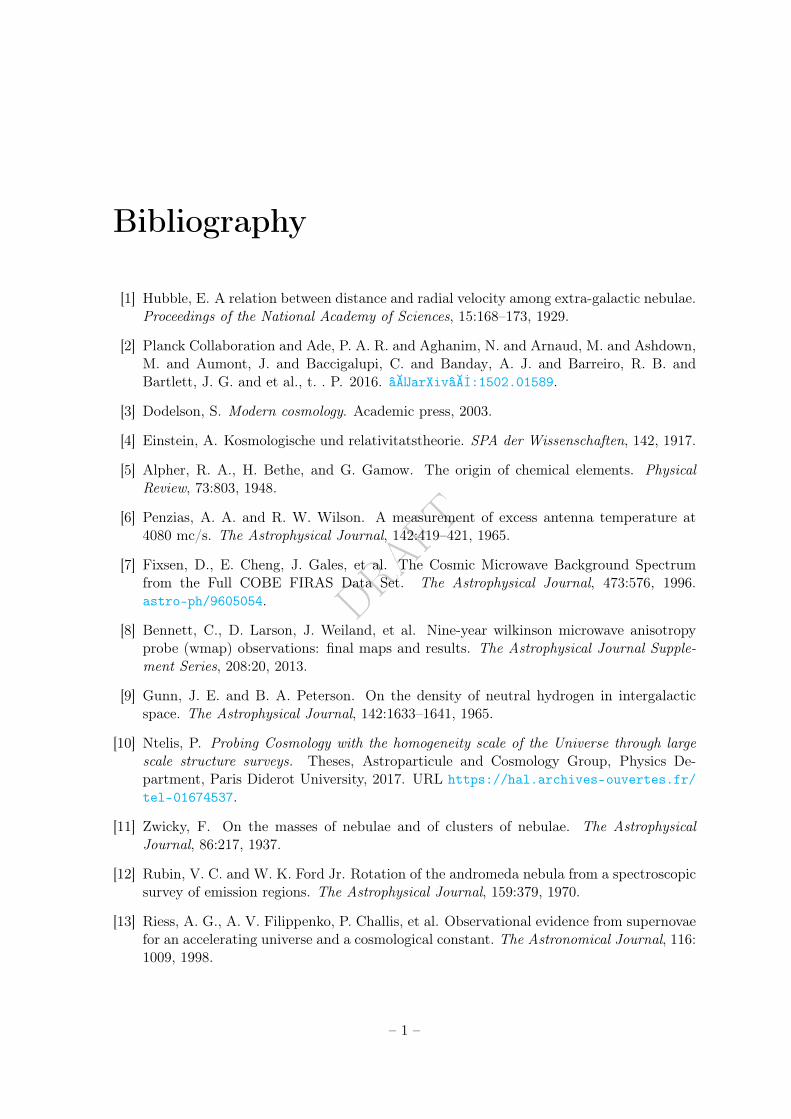
DRAFT

Bibliography

[1] Hubble, E. A relation between distance and radial velocity among extra-galactic nebulae.Proceedings of the National Academy of Sciences, 15:168–173, 1929.

[2] Planck Collaboration and Ade, P. A. R. and Aghanim, N. and Arnaud, M. and Ashdown,M. and Aumont, J. and Baccigalupi, C. and Banday, A. J. and Barreiro, R. B. andBartlett, J. G. and et al., t. . P. 2016. âĂIJarXivâĂİ:1502.01589.

[3] Dodelson, S. Modern cosmology. Academic press, 2003.

[4] Einstein, A. Kosmologische und relativitatstheorie. SPA der Wissenschaften, 142, 1917.

[5] Alpher, R. A., H. Bethe, and G. Gamow. The origin of chemical elements. PhysicalReview, 73:803, 1948.

[6] Penzias, A. A. and R. W. Wilson. A measurement of excess antenna temperature at4080 mc/s. The Astrophysical Journal, 142:419–421, 1965.

[7] Fixsen, D., E. Cheng, J. Gales, et al. The Cosmic Microwave Background Spectrumfrom the Full COBE FIRAS Data Set. The Astrophysical Journal, 473:576, 1996.astro-ph/9605054.

[8] Bennett, C., D. Larson, J. Weiland, et al. Nine-year wilkinson microwave anisotropyprobe (wmap) observations: final maps and results. The Astrophysical Journal Supple-ment Series, 208:20, 2013.

[9] Gunn, J. E. and B. A. Peterson. On the density of neutral hydrogen in intergalacticspace. The Astrophysical Journal, 142:1633–1641, 1965.

[10] Ntelis, P. Probing Cosmology with the homogeneity scale of the Universe through largescale structure surveys. Theses, Astroparticule and Cosmology Group, Physics De-partment, Paris Diderot University, 2017. URL https://hal.archives-ouvertes.fr/tel-01674537.

[11] Zwicky, F. On the masses of nebulae and of clusters of nebulae. The AstrophysicalJournal, 86:217, 1937.

[12] Rubin, V. C. and W. K. Ford Jr. Rotation of the andromeda nebula from a spectroscopicsurvey of emission regions. The Astrophysical Journal, 159:379, 1970.

[13] Riess, A. G., A. V. Filippenko, P. Challis, et al. Observational evidence from supernovaefor an accelerating universe and a cosmological constant. The Astronomical Journal, 116:1009, 1998.

– 1 –

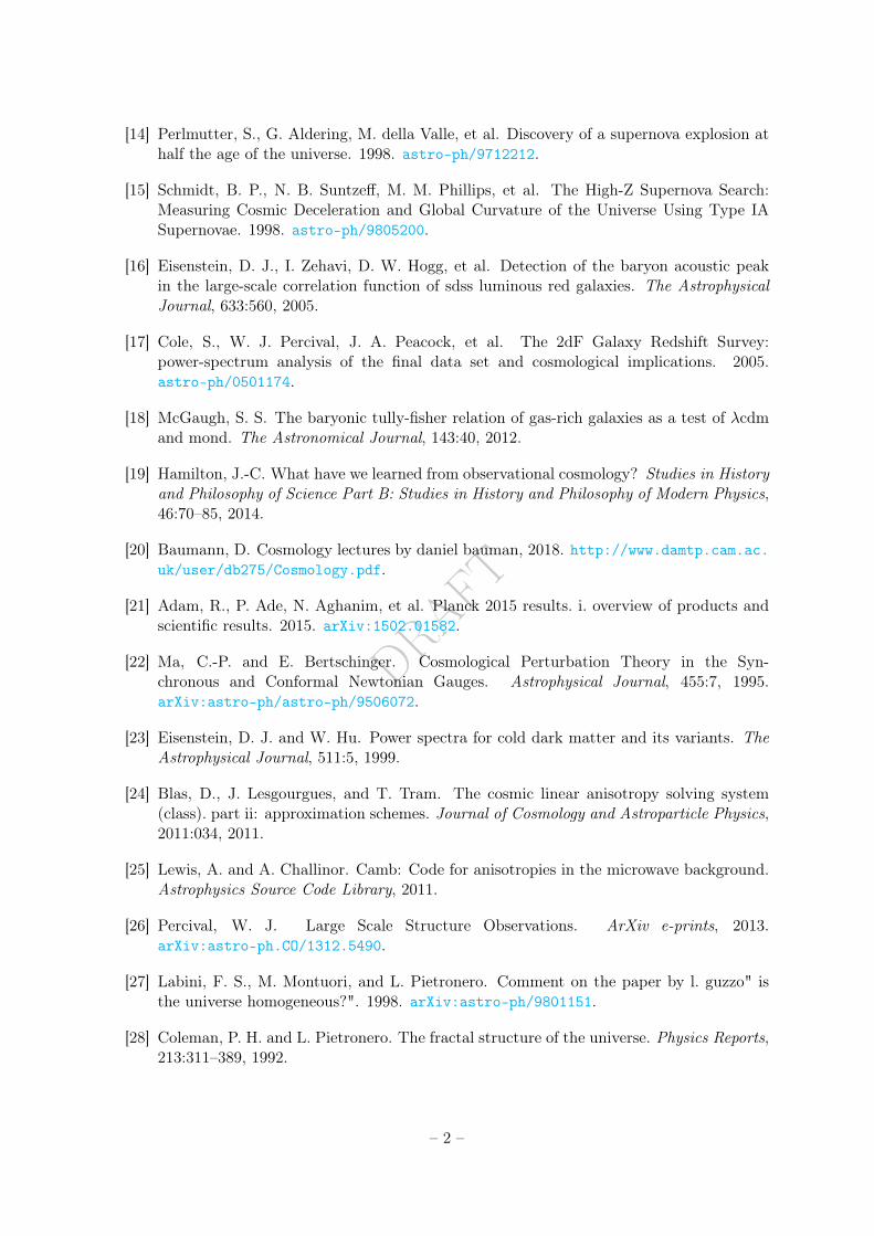
DRAFT

[14] Perlmutter, S., G. Aldering, M. della Valle, et al. Discovery of a supernova explosion athalf the age of the universe. 1998. astro-ph/9712212.

[15] Schmidt, B. P., N. B. Suntzeff, M. M. Phillips, et al. The High-Z Supernova Search:Measuring Cosmic Deceleration and Global Curvature of the Universe Using Type IASupernovae. 1998. astro-ph/9805200.

[16] Eisenstein, D. J., I. Zehavi, D. W. Hogg, et al. Detection of the baryon acoustic peakin the large-scale correlation function of sdss luminous red galaxies. The AstrophysicalJournal, 633:560, 2005.

[17] Cole, S., W. J. Percival, J. A. Peacock, et al. The 2dF Galaxy Redshift Survey:power-spectrum analysis of the final data set and cosmological implications. 2005.astro-ph/0501174.

[18] McGaugh, S. S. The baryonic tully-fisher relation of gas-rich galaxies as a test of λcdmand mond. The Astronomical Journal, 143:40, 2012.

[19] Hamilton, J.-C. What have we learned from observational cosmology? Studies in Historyand Philosophy of Science Part B: Studies in History and Philosophy of Modern Physics,46:70–85, 2014.

[20] Baumann, D. Cosmology lectures by daniel bauman, 2018. http://www.damtp.cam.ac.uk/user/db275/Cosmology.pdf.

[21] Adam, R., P. Ade, N. Aghanim, et al. Planck 2015 results. i. overview of products andscientific results. 2015. arXiv:1502.01582.

[22] Ma, C.-P. and E. Bertschinger. Cosmological Perturbation Theory in the Syn-chronous and Conformal Newtonian Gauges. Astrophysical Journal, 455:7, 1995.arXiv:astro-ph/astro-ph/9506072.

[23] Eisenstein, D. J. and W. Hu. Power spectra for cold dark matter and its variants. TheAstrophysical Journal, 511:5, 1999.

[24] Blas, D., J. Lesgourgues, and T. Tram. The cosmic linear anisotropy solving system(class). part ii: approximation schemes. Journal of Cosmology and Astroparticle Physics,2011:034, 2011.

[25] Lewis, A. and A. Challinor. Camb: Code for anisotropies in the microwave background.Astrophysics Source Code Library, 2011.

[26] Percival, W. J. Large Scale Structure Observations. ArXiv e-prints, 2013.arXiv:astro-ph.CO/1312.5490.

[27] Labini, F. S., M. Montuori, and L. Pietronero. Comment on the paper by l. guzzo" isthe universe homogeneous?". 1998. arXiv:astro-ph/9801151.

[28] Coleman, P. H. and L. Pietronero. The fractal structure of the universe. Physics Reports,213:311–389, 1992.

– 2 –

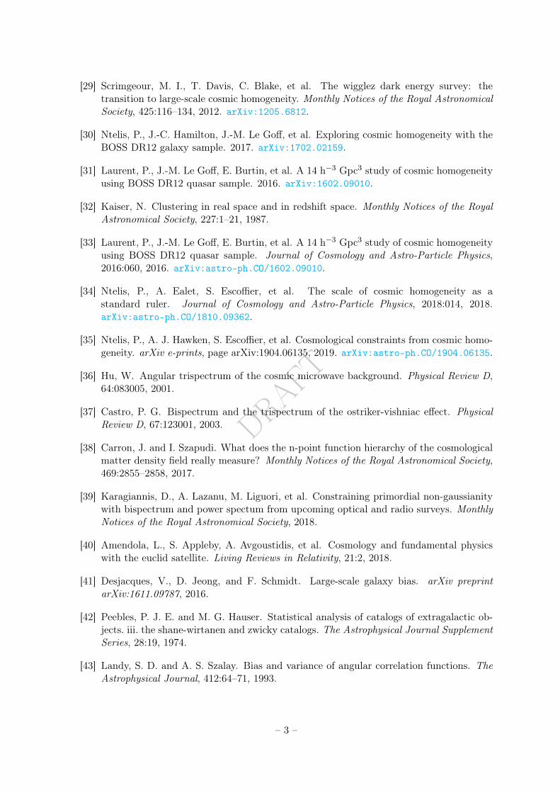
DRAFT

[29] Scrimgeour, M. I., T. Davis, C. Blake, et al. The wigglez dark energy survey: thetransition to large-scale cosmic homogeneity. Monthly Notices of the Royal AstronomicalSociety, 425:116–134, 2012. arXiv:1205.6812.

[30] Ntelis, P., J.-C. Hamilton, J.-M. Le Goff, et al. Exploring cosmic homogeneity with theBOSS DR12 galaxy sample. 2017. arXiv:1702.02159.

[31] Laurent, P., J.-M. Le Goff, E. Burtin, et al. A 14 h−3 Gpc3 study of cosmic homogeneityusing BOSS DR12 quasar sample. 2016. arXiv:1602.09010.

[32] Kaiser, N. Clustering in real space and in redshift space. Monthly Notices of the RoyalAstronomical Society, 227:1–21, 1987.

[33] Laurent, P., J.-M. Le Goff, E. Burtin, et al. A 14 h−3 Gpc3 study of cosmic homogeneityusing BOSS DR12 quasar sample. Journal of Cosmology and Astro-Particle Physics,2016:060, 2016. arXiv:astro-ph.CO/1602.09010.

[34] Ntelis, P., A. Ealet, S. Escoffier, et al. The scale of cosmic homogeneity as astandard ruler. Journal of Cosmology and Astro-Particle Physics, 2018:014, 2018.arXiv:astro-ph.CO/1810.09362.

[35] Ntelis, P., A. J. Hawken, S. Escoffier, et al. Cosmological constraints from cosmic homo-geneity. arXiv e-prints, page arXiv:1904.06135, 2019. arXiv:astro-ph.CO/1904.06135.

[36] Hu, W. Angular trispectrum of the cosmic microwave background. Physical Review D,64:083005, 2001.

[37] Castro, P. G. Bispectrum and the trispectrum of the ostriker-vishniac effect. PhysicalReview D, 67:123001, 2003.

[38] Carron, J. and I. Szapudi. What does the n-point function hierarchy of the cosmologicalmatter density field really measure? Monthly Notices of the Royal Astronomical Society,469:2855–2858, 2017.

[39] Karagiannis, D., A. Lazanu, M. Liguori, et al. Constraining primordial non-gaussianitywith bispectrum and power spectum from upcoming optical and radio surveys. MonthlyNotices of the Royal Astronomical Society, 2018.

[40] Amendola, L., S. Appleby, A. Avgoustidis, et al. Cosmology and fundamental physicswith the euclid satellite. Living Reviews in Relativity, 21:2, 2018.

[41] Desjacques, V., D. Jeong, and F. Schmidt. Large-scale galaxy bias. arXiv preprintarXiv:1611.09787, 2016.

[42] Peebles, P. J. E. and M. G. Hauser. Statistical analysis of catalogs of extragalactic ob-jects. iii. the shane-wirtanen and zwicky catalogs. The Astrophysical Journal SupplementSeries, 28:19, 1974.

[43] Landy, S. D. and A. S. Szalay. Bias and variance of angular correlation functions. TheAstrophysical Journal, 412:64–71, 1993.

– 3 –

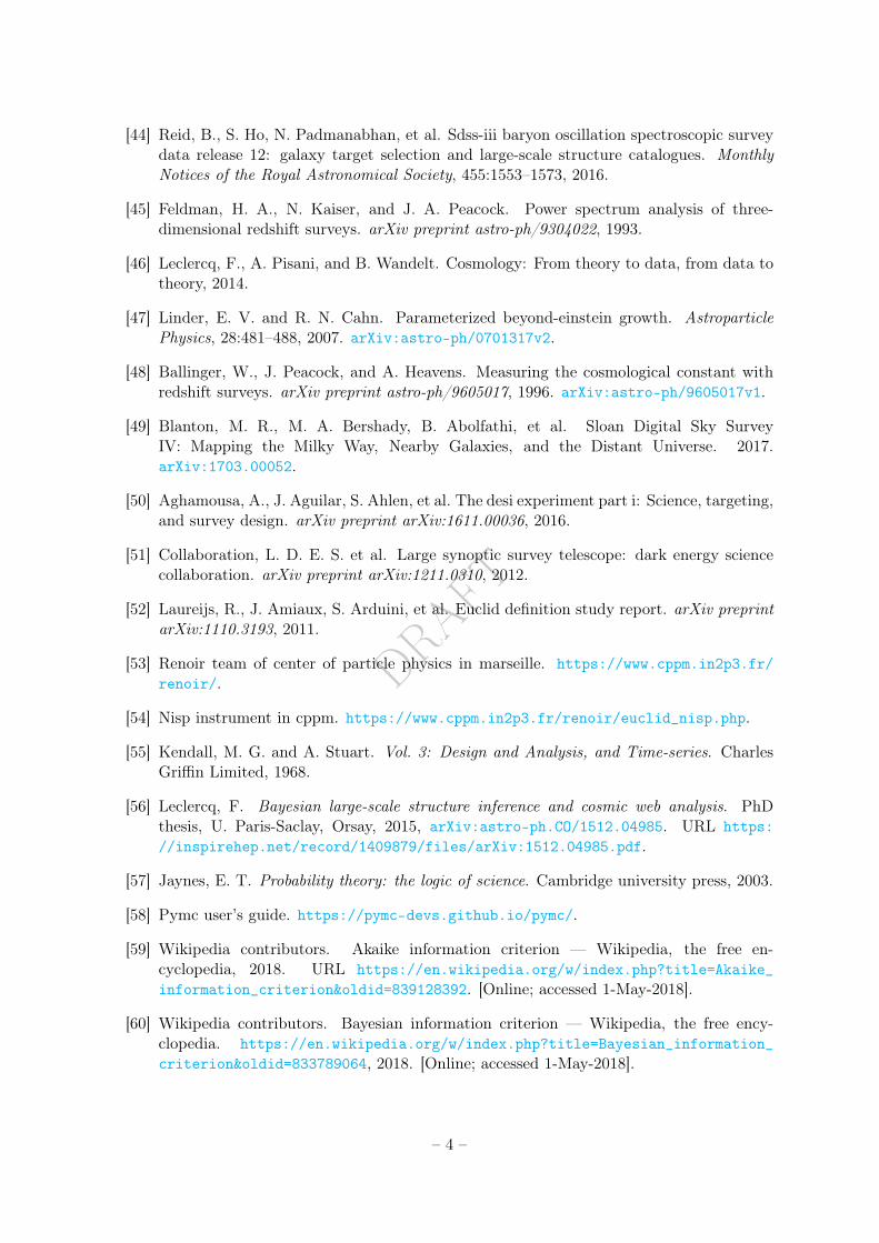
DRAFT

[44] Reid, B., S. Ho, N. Padmanabhan, et al. Sdss-iii baryon oscillation spectroscopic surveydata release 12: galaxy target selection and large-scale structure catalogues. MonthlyNotices of the Royal Astronomical Society, 455:1553–1573, 2016.

[45] Feldman, H. A., N. Kaiser, and J. A. Peacock. Power spectrum analysis of three-dimensional redshift surveys. arXiv preprint astro-ph/9304022, 1993.

[46] Leclercq, F., A. Pisani, and B. Wandelt. Cosmology: From theory to data, from data totheory, 2014.

[47] Linder, E. V. and R. N. Cahn. Parameterized beyond-einstein growth. AstroparticlePhysics, 28:481–488, 2007. arXiv:astro-ph/0701317v2.

[48] Ballinger, W., J. Peacock, and A. Heavens. Measuring the cosmological constant withredshift surveys. arXiv preprint astro-ph/9605017, 1996. arXiv:astro-ph/9605017v1.

[49] Blanton, M. R., M. A. Bershady, B. Abolfathi, et al. Sloan Digital Sky SurveyIV: Mapping the Milky Way, Nearby Galaxies, and the Distant Universe. 2017.arXiv:1703.00052.

[50] Aghamousa, A., J. Aguilar, S. Ahlen, et al. The desi experiment part i: Science, targeting,and survey design. arXiv preprint arXiv:1611.00036, 2016.

[51] Collaboration, L. D. E. S. et al. Large synoptic survey telescope: dark energy sciencecollaboration. arXiv preprint arXiv:1211.0310, 2012.

[52] Laureijs, R., J. Amiaux, S. Arduini, et al. Euclid definition study report. arXiv preprintarXiv:1110.3193, 2011.

[53] Renoir team of center of particle physics in marseille. https://www.cppm.in2p3.fr/renoir/.

[54] Nisp instrument in cppm. https://www.cppm.in2p3.fr/renoir/euclid_nisp.php.

[55] Kendall, M. G. and A. Stuart. Vol. 3: Design and Analysis, and Time-series. CharlesGriffin Limited, 1968.

[56] Leclercq, F. Bayesian large-scale structure inference and cosmic web analysis. PhDthesis, U. Paris-Saclay, Orsay, 2015, arXiv:astro-ph.CO/1512.04985. URL https://inspirehep.net/record/1409879/files/arXiv:1512.04985.pdf.

[57] Jaynes, E. T. Probability theory: the logic of science. Cambridge university press, 2003.

[58] Pymc user’s guide. https://pymc-devs.github.io/pymc/.

[59] Wikipedia contributors. Akaike information criterion — Wikipedia, the free en-cyclopedia, 2018. URL https://en.wikipedia.org/w/index.php?title=Akaike_information_criterion&oldid=839128392. [Online; accessed 1-May-2018].

[60] Wikipedia contributors. Bayesian information criterion — Wikipedia, the free ency-clopedia. https://en.wikipedia.org/w/index.php?title=Bayesian_information_criterion&oldid=833789064, 2018. [Online; accessed 1-May-2018].

– 4 –

DRAFT

[61] Wikipedia contributors. Spline (mathematics) — Wikipedia, the free encyclopedia,2018. URL https://en.wikipedia.org/w/index.php?title=Spline_(mathematics)&oldid=837660470. [Online; accessed 1-May-2018].

[62] Wikipedia contributors. Metropolis?hastings algorithm — Wikipedia, the free encyclo-pedia, 2018. URL https://en.wikipedia.org/w/index.php?title=Metropolis%E2%80%93Hastings_algorithm&oldid=838047823. [Online; accessed 11-May-2018].

[63] Roberts, G. O., A. Gelman, W. R. Gilks, et al. Weak convergence and optimal scaling ofrandom walk metropolis algorithms. The annals of applied probability, 7:110–120, 1997.

[64] Gelman, A. and D. B. Rubin. Inference from iterative simulation using multiple se-quences. Statist. Sci., 7:457–472, 1992.

[65] Heidelberger, P. and P. D. Welch. A spectral method for confidence interval generationand run length control in simulations. Communications of the ACM, 24:233–245, 1981.

[66] Goodman, J., J. Weare, et al. Ensemble samplers with affine invariance. Communicationsin applied mathematics and computational science, 5:65–80, 2010.

[67] Doux, C. Combinations of cosmological probes: two applications with data from Planckand SDSS-III/BOSS. PhD thesis, APC, Paris, 2017. http://inspirehep.net/record/1665198/files/fulltext.pdf.

– 5 –