0

A Novel Approach for Mathematically

Modeling Pretargeted Radioimmunotherapy

Using Hapten Radionuclides as Treatments for Colon Cancer

Ananth Ram Graduate of the Texas Academy of Mathematics and Science, 2008 Research performed at home and at the Massachusetts Institute of

Technology, Wittrup Labs

1

I. Personal My first exposure to biomedical engineering occurred four years ago when I attended an engineering camp

at the University of Texas at Arlington. The professor who conducted the camp was researching biological

scaffolding and its application to re-growing damaged tissue. He talked about how he used lactic acid (a byproduct

of anaerobic respiration of cells, the burning sensation people feel in their muscles after they have been exercising

for too long) to create an organic polymer, which he used to re-grow damaged nerve endings in the legs of mice,

enabling them to use their legs again. This was just a small part of the diverse field of biomedical engineering, and

I was hooked.

Three years later, I applied to the Research Science Institute, a summer research program for incoming

high school seniors held at the Massachusetts Institute of Technology, looking for an opportunity to do research in

nanotechnology or biomedical engineering. I was assigned a project at the Wittrup Labs in the

biomedical/chemical engineering departments. The lab was working on a way to engineer proteins to use in pre-

targeted radio immunotherapy, a type of cancer treatment that uses antibodies to target only cancer cells while

leaving normal cells unharmed. The goal was to eventually use the engineered antibodies to treat colon cancer.

The experimental team was working on more efficient ways to synthesize the protein, while the theoretical team

was working on how to simulate the cancer treatment in different conditions in order to predict outcomes. I

worked with the theoretical team to mathematically model the protein interactions and relevant processes to

predict the results of the treatment. My specific assignment was to design a model that looked at the effects of the

treatment on normal colon tissue, as antibodies will also attach to normal colon cells.

A system of differential equations describes the change in concentration over time of antibodies, antigens

(cell surface markers that identify cancer cells and normal cells), hapten (radioactive molecules that attach to the

cancer cell-specific antibodies, dosing only the cells with radiation), and antibody/antigen/hapten complexes.

Since my work would involve differential equations, I learned some basic techniques to solve linear differential

equations. The system of equations did not yield to analytical solutions and required numerical techniques for

solution. Since I had exposure in using MATLAB, a programming language and interface that provides toolboxes

that aid in solving mathematical problems, I saw an opportunity in this project to use it in solving the system of

differential equations. I wrote a program simulating how cells grow in colon tissue and used a differential

equations solver in MATLAB to solve the differential equations in the model. Even though the system of

equations was complex, I was successful in applying MATLAB to find solutions and extrapolations which I was

able to use in predicting optimum times to dose the radiation or the antibodies, in order to minimize damage done

to normal colon tissue. I had not had much in-depth experience in applied math before and this project provided

2

me with an opportunity to learn about the myriad of applications of mathematics in many other areas of science,

and to actually use new techniques to solve biological and engineering problems.. For me, mathematics will always

be the language of the sciences, and my work in this project only strengthened my desire to pursue engineering, a

balanced combination of mathematics and science.

My advice to other high school students who wish to pursue math and science is to never feel intimidated.

Problem solving techniques in engineering and science involve application of mathematics spanning various facets,

such as statistics to calculus to abstract algebra and topology. When it becomes necessary to learn and apply them,

do not feel intimidated by their complexity; it may be hard to understand some of these concepts at first, but it is

important to be persistent. A sudden epiphany is all it takes for it to click, and it can occur at any time, as long as

you have been doing all you can to expand your boundaries and learn all there is to learn about the fundamental

concepts. Though you may experience stumbles or setbacks, it is imperative to never give up during the process;

eventually everything will fall into place. The time spent learning and applying the math, creatively coming up with

methods to solve the problem at hand, is the most fun time one can spend in a project. Be creative, explore all the

options, and have fun while doing it.

II. Research

1. Rationale

Conventional treatments for cancerous tumors include chemotherapy, radiation therapy, and surgery.

However, the success of these treatments varies, and there are many dangerous side effects, including the loss of

other organ functions and death of healthy cells [11]. A promising alternative treatment is pre-targeted

radioimmunotherapy (pRIT), a process in which antibodies are used to target tumor cells and subsequently recruit

a small radioactive chelating molecule known as a hapten to those specific cells, killing them without harming

normal body cells [8]. However, a majority of previous clinical trials of antibody therapeutics have met with

failure, partly because of the inability of the doctors and scientists to determine the optimum conditions for the

interactions between antibodies and antigens in clinical trials.

When scientists conduct clinical trials, it is important that the correct dosages for the drug are

administered, as the researchers may have absolutely no idea of the outcomes or side-effects of drugs when they

are first tested in humans. One important method of extrapolating results lies in mathematical modeling. With a

3

model, scientists can provide reasonably accurate predictions through computer simulations. This will in turn save

time and money in order to produce the most informative and effective clinical trials possible while mitigating

toxicities [8].

The purpose of this project is to model the interactions of antibodies with antigens (cell identifier

proteins) expressed on the surfaces of tumor cells found in the colon. The second goal is to successfully simulate

the colon system to determine the correct dose of hapten nuclides needed to completely kill a cancerous tumor.

The final goal is to model alpha particle emission and its effects in the treatment process. In order to model these

pharmacokinetic and pharmacodynamic processes, it is necessary to derive mathematical relationships. The model

in this paper was derived from data acquired from experiments as well as kinetics laws relating to diffusivity, fluid

dynamics, and non-covalent attractions [15]. The generalized model portrays the interactions of various antibodies

and antigens in order to identify the certain conditions that need to be met for pRIT to be successful. The model

will be useful to the medical community in order to calculate correct doses of antibodies and haptens and analyze

the effects of various substances in order to plan more effective and more informative clinical trials.

Three studies were conducted. The first involved analyzing the current pRIT model and fixing any

inefficiencies or redundancies. This also involved running the simulation many times with different parameters in

order to calculate the optimum conditions for dosing the antibodies and the hapten. The second study dealt with

creating a new model that simulated pRIT involving the A33 antigen in the colon. This study involved modeling

the physiology of the colon and the migration of cells in order to take into account antibodies binding to healthy

body cells. The final study dealt with creating a successful model of alpha particle decay in order to incorporate

into the primary pRIT dosimetry simulation.

2. Prior Work

Research has been conducted dealing with two specific antigens found on the cells in the colon, A33 and

CEA. Two antibody formats are also being studied: IgG (human immunoglobulin G) and scFv (single chain

variable fragment). Researchers have built a mathematical model that identifies the rates of change of

concentrations of the antibody, antigen, hapten, and antibody/antigen bound complexes [7, 11]. The model also

incorporates radiation dosimetry and calculations of hapten dosage times and half-life decay.

pRIT, a subset of radioimmunotherapy (RIT), deals with antibody/antigen interactions. Tumor cells

express certain antigens on their surfaces. There are certain antibodies that will attach to specific antigens.

Scientists can engineer these antibodies to act as tags as they attach to the surfaces of tumor cells [1, 9]. Then, at

an optimum time, the radioactive hapten is injected into the system and will attach to the antibodies and thereby

4

dose the cell with radiation. Normal radioimmunotherapy (RIT) is similar in concept: the only difference is that

the antibody is initially attached to the hapten before it is injected into the bloodstream, thereby dosing the tumor

cell with radiation through a single injection. The shortcomings of RIT, however, cause RIT to be less successful

than pRIT. Because the hapten is attached to the antibody, the entire antibody hapten complex is much larger and

more complex of a structure than the antibody alone, and because of its relatively immense size, it flows through

the bloodstream at a much slower pace. More of the body system is exposed to the radiation emitted from the

attached hapten for a longer period of time, which can pose a greater risk of ill side effects than regular radiation

therapy [1]. pRIT eliminates this risk as the separate antibody and hapten fragments flow in and out of the

bloodstream at a much quicker pace.

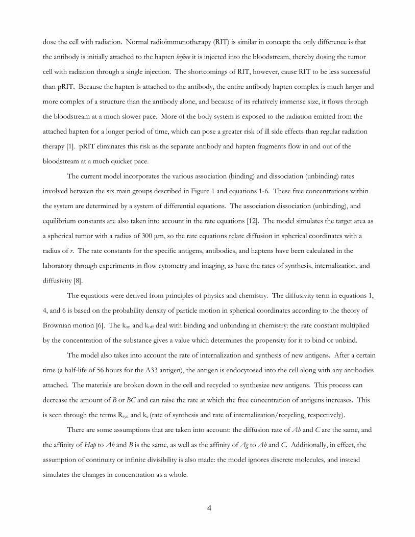
The current model incorporates the various association (binding) and dissociation (unbinding) rates

involved between the six main groups described in Figure 1 and equations 1-6. These free concentrations within

the system are determined by a system of differential equations. The association dissociation (unbinding), and

equilibrium constants are also taken into account in the rate equations [12]. The model simulates the target area as

a spherical tumor with a radius of 300 µm, so the rate equations relate diffusion in spherical coordinates with a

radius of r. The rate constants for the specific antigens, antibodies, and haptens have been calculated in the

laboratory through experiments in flow cytometry and imaging, as have the rates of synthesis, internalization, and

diffusivity [8].

The equations were derived from principles of physics and chemistry. The diffusivity term in equations 1,

4, and 6 is based on the probability density of particle motion in spherical coordinates according to the theory of

Brownian motion [6]. The kon and koff deal with binding and unbinding in chemistry: the rate constant multiplied

by the concentration of the substance gives a value which determines the propensity for it to bind or unbind.

The model also takes into account the rate of internalization and synthesis of new antigens. After a certain

time (a half-life of 56 hours for the A33 antigen), the antigen is endocytosed into the cell along with any antibodies

attached. The materials are broken down in the cell and recycled to synthesize new antigens. This process can

decrease the amount of B or BC and can raise the rate at which the free concentration of antigens increases. This

is seen through the terms Rsyn and ke (rate of synthesis and rate of internalization/recycling, respectively).

There are some assumptions that are taken into account: the diffusion rate of Ab and C are the same, and

the affinity of Hap to Ab and B is the same, as well as the affinity of Ag to Ab and C. Additionally, in effect, the

assumption of continuity or infinite divisibility is also made: the model ignores discrete molecules, and instead

simulates the changes in concentration as a whole.

5

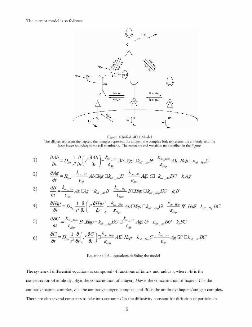
The system of differential equations is composed of functions of time t and radius r, where Ab is the

concentration of antibody, Ag is the concentration of antigen, Hap is the concentration of hapten, C is the

antibody/hapten complex, B is the antibody/antigen complex, and BC is the antibody/hapten/antigen complex.

There are also several constants to take into account: D is the diffusivity constant for diffusion of particles in

Equations 1-6 – equations defining the model

1)

2)

3)

4)

5)

6)

ε ε

ε ε

ε ε

∂ ∂ ∂ = − ⋅ + − ⋅ + ∂ ∂ ∂

∂ = − ⋅ + − ⋅ + −∂

∂ = ⋅ − − ⋅ + −∂

_ _2_ _2

_ _

_ _

_ _

_ _

1 on Ab on HapAb off Ab off Hap

Ab Hap

on Ab on Absyn off Ab off Ab e

Ab Ab

on Ab on Hapoff Ab off Hap

Ab Hap

k kAb AbD r Ab Ag k B Ab Hap k C

t r r r

k kAgR Ab Ag k B Ag C k BC k Ag

t

k kBAb Ag k B B Hap k BC

t

ε ε

ε ε

ε

∂ ∂ ∂ = − ⋅ + − ⋅ + ∂ ∂ ∂

∂ = ⋅ − + ⋅ − −∂

∂ ∂ ∂ = + ⋅ − ∂ ∂ ∂

_ _2_ _2

_ _

_ _

_2

2

1

1

e

on Hap on HapHap off Hap off Hap

Hap Hap

on Hap on Aboff Hap off Ab e

Hap Ab

on HapAb of

Hap

k B

k kHap HapD r Ab Hap k C B Hap k BC

t r r r

k kBCB Hap k BC Ag C k BC k BC

t

kC CD r Ab Hap k

t r r r ε− ⋅ +_

_ _

on Abf Hap off Ab

Ab

kC Ag C k BC

The current model is as follows:

Figure 1-Initial pRIT Model The ellipses represent the hapten, the triangles represent the antigen, the complex fork represents the antibody, and the

large lower boundary is the cell membrane. The constants and variables are described in the Figure

6

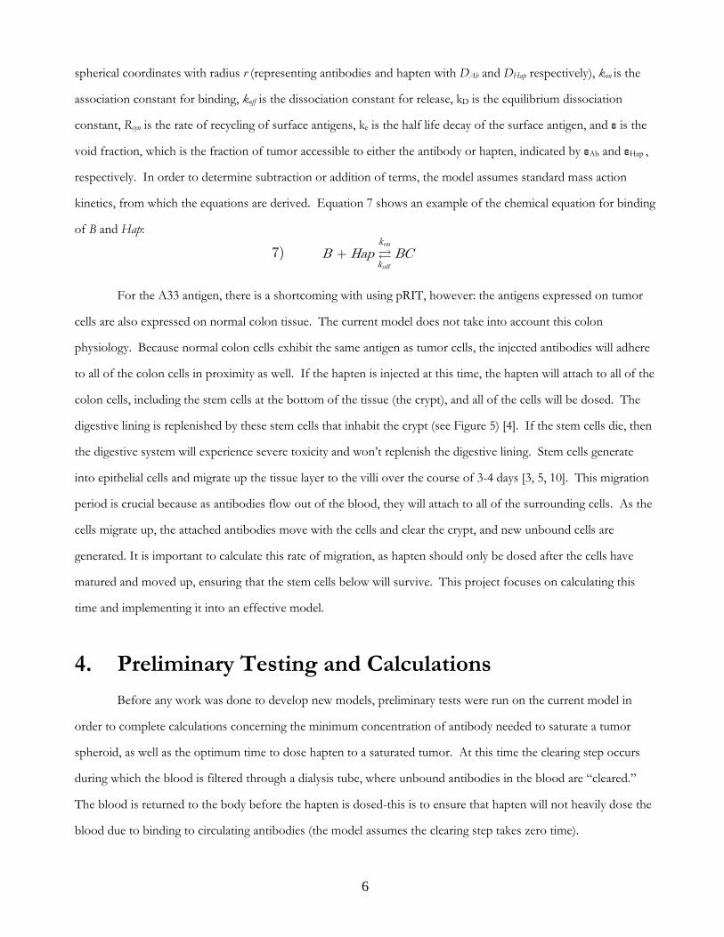
spherical coordinates with radius r (representing antibodies and hapten with DAb and DHap respectively), kon is the

association constant for binding, koff is the dissociation constant for release, kD is the equilibrium dissociation

constant, Rsyn is the rate of recycling of surface antigens, ke is the half life decay of the surface antigen, and ε is the

void fraction, which is the fraction of tumor accessible to either the antibody or hapten, indicated by εAb and εHap ,

respectively. In order to determine subtraction or addition of terms, the model assumes standard mass action

kinetics, from which the equations are derived. Equation 7 shows an example of the chemical equation for binding

of B and Hap:

For the A33 antigen, there is a shortcoming with using pRIT, however: the antigens expressed on tumor

cells are also expressed on normal colon tissue. The current model does not take into account this colon

physiology. Because normal colon cells exhibit the same antigen as tumor cells, the injected antibodies will adhere

to all of the colon cells in proximity as well. If the hapten is injected at this time, the hapten will attach to all of the

colon cells, including the stem cells at the bottom of the tissue (the crypt), and all of the cells will be dosed. The

digestive lining is replenished by these stem cells that inhabit the crypt (see Figure 5) [4]. If the stem cells die, then

the digestive system will experience severe toxicity and won’t replenish the digestive lining. Stem cells generate

into epithelial cells and migrate up the tissue layer to the villi over the course of 3-4 days [3, 5, 10]. This migration

period is crucial because as antibodies flow out of the blood, they will attach to all of the surrounding cells. As the

cells migrate up, the attached antibodies move with the cells and clear the crypt, and new unbound cells are

generated. It is important to calculate this rate of migration, as hapten should only be dosed after the cells have

matured and moved up, ensuring that the stem cells below will survive. This project focuses on calculating this

time and implementing it into an effective model.

4. Preliminary Testing and Calculations

Before any work was done to develop new models, preliminary tests were run on the current model in

order to complete calculations concerning the minimum concentration of antibody needed to saturate a tumor

spheroid, as well as the optimum time to dose hapten to a saturated tumor. At this time the clearing step occurs

during which the blood is filtered through a dialysis tube, where unbound antibodies in the blood are “cleared.”

The blood is returned to the body before the hapten is dosed-this is to ensure that hapten will not heavily dose the

blood due to binding to circulating antibodies (the model assumes the clearing step takes zero time).

7) on

off

k

kB Hap BC+ �

7

4.1 Minimum Antibody Concentration for Saturation

The time of saturation is defined as the first point at which the most amount of antigen in the tumor (at all

distances along the radius) has been bound by antibodies. According to mass action kinetics, there will never be a

point at which all the antigens are bound because the rate at which antigens bind decreases as the free antigens

decreases. Due to this exponential decay, there will always be some free antigen. The point of saturation is a

necessary consideration in order to calculate the minimum concentration of antibody needed to saturate a tumor.

It would be inefficient to dose hapten and run the clearing step when the tumor is not saturated because not all of

the tumor would be dosed, and the injection would be wasted. It is also important that the amount of antibodies

dosed is minimized. In order to minimize the risk of trials similar to TGN1412, it is important to give as low a

dose of antibodies as possible, but still have enough for a full saturation (in order to maintain maximum

efficiency). This test seeks to reduce the dose from the minimum safe concentration used in previous clinical tests

of 200nM [13] to a range in which the tumor will still become saturated with antibodies.

Initial tests were run with antibody concentration at 80 x 10-9 M for each of the A33 and CEA antigens.

Then, depending on whether the tumor reached saturation at the center, the initial antibody concentration was

increased or decreased at the start of each set of tests. For example, both IgG and scFv saturated the A33 antigen

at 80 x 10-9 M concentration, so the concentration was reduced to 80 x 10-10 M. There, the antibodies did not

saturate, so the concentration was increased to 40 x 10-9 M. This recursive method continued the final

concentration was within a 10 x 10-9 M range. The simulation was run for 240 hours for A33, but was run for

anywhere between 48 and 96 hours for CEA due to the shorter half life of the CEA antigen. Table 1 shows the

results of the tests:

Minimum Antibody Concentration Range for Saturation

IgG scFv

A33 50 x 10-9 to 60 x 10-9 M 70 x 10-9 to 80 x 10-9 M

CEA 130 x 10-9 to 140 x 10-9 M 120 x 10-9 to 130 x 10-9 M

This method was also done for the CEA antigen. The antibody fails to penetrate to the center of the

tumor because the half-life of CEA is 12 hours while A33’s is 56 hours. This effect is known as the “binding site

barrier.” Antibodies cannot bind further into a tumor spheroid unless all possible antigens on one layer of cells are

bound. Only then can the antibodies penetrate to the next layer. The lower value for DAb combined with the fast

Table 1

8

kon rate account for the binding site barrier. Binding is faster than diffusion, therefore no antibody diffuses past an

empty binding site. Binding sites are thus filled in order from outside to inside. For CEA, the antibodies will fail

to penetrate because the turnover rate (decay of antigen) is equivalent to the antibody diffusion. The antibody will

bind to the outside of the tumor and will start working inward, but meanwhile, the antigen on the outside is

internalized, degraded, and replaced by new antigen that will bind the next antibody that begins to diffuse into the

tumor. Because none of the antibodies saturated while binding to CEA initially, the concentrations were increased,

then the recursive method was implemented until the final concentration was within a 10 x 10-9 M range.

4.2 Optimum Hapten Dosage Time

After the optimum antibody doses were found, the test for calculating optimum hapten dosage times was

run for these antibody concentrations. It is important that hapten be dosed at the right time. If dosed too early,

then hapten will bind with stray antibodies in the blood, causing nearby body tissue to be irradiated. If dosed too

late, then there will be fewer antibody/antigen complexes to attach to, due to the half-life decay of the surface

antigens, and efficiency is lost. Therefore, the optimum time to dose the hapten would be when the overall

concentration of bound antibodies throughout the tumor is at the maximum.

A function was added to the model that would calculate cumulative antibody concentration as a function

of time across the radius of the tumor spheroid for each timestep (effectively “slices” of the output for each time).

The function would then compare all of the areas and return the cumulative concentration (represented as the area

under the curve), as well as the timestep for that area. Equation 8 describes the integration calculation involved:

where 4̟ r2 Ab represents the calculation of the area for that concentration at the specific time, while the function

integrates from 0 to r. This was then translated into MATLAB code:

for p = 1:length(t)

opt(p) = quad(@optimum_time,0,Param.R_tumor,[],[],F,r_axis,p);

end

[opt_max,index] = max(opt);

t_max = t(index)

t_max/3600 ...

function A = optimum_time(r,F,r_axis,p)

A = interp1(r_axis,F(p,:),r);

return; ...

2

0

4

r

r Ab drπ∫8)

9

The function “quad” computes integral from 0 to the radius of the tumor of “optimum_time,” and passes the

variables F (total bound antibody), r_axis (radius axis), and p (for each step along the length of time). The function

“optimum_time” passes r, F, and p, and interpolates along the radius axis so that all concentrations in between the

timesteps are taken into account.

The time returned is the first time at which the area is greatest, and therefore the first time at which the

entire tumor is saturated completely, thus delivering the ideal conditions for hapten dosing. The reason that the

area under the curve is considered, rather than an absolute maximum point, is that at a given time t = n, the outside

edge of the tumor might be completely saturated (at the maximum point), yet the inside might be empty. Then at a

given time t = n + k, the outside edge might not be as saturated, yet the antibody concentration might have

increased significantly at the center of the tumor. It is better to dose the hapten at this point because of greater

overall tumor coverage.

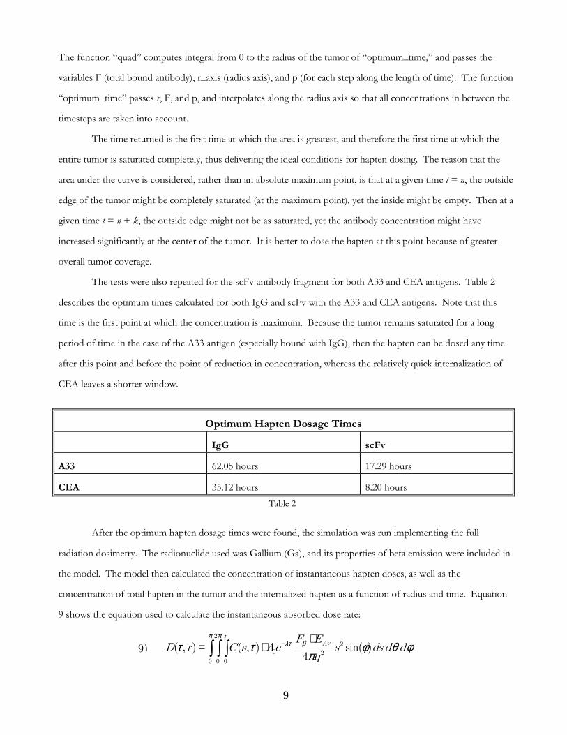
The tests were also repeated for the scFv antibody fragment for both A33 and CEA antigens. Table 2

describes the optimum times calculated for both IgG and scFv with the A33 and CEA antigens. Note that this

time is the first point at which the concentration is maximum. Because the tumor remains saturated for a long

period of time in the case of the A33 antigen (especially bound with IgG), then the hapten can be dosed any time

after this point and before the point of reduction in concentration, whereas the relatively quick internalization of

CEA leaves a shorter window.

Optimum Hapten Dosage Times

IgG scFv

A33 62.05 hours 17.29 hours

CEA 35.12 hours 8.20 hours

After the optimum hapten dosage times were found, the simulation was run implementing the full

radiation dosimetry. The radionuclide used was Gallium (Ga), and its properties of beta emission were included in

the model. The model then calculated the concentration of instantaneous hapten doses, as well as the

concentration of total hapten in the tumor and the internalized hapten as a function of radius and time. Equation

9 shows the equation used to calculate the instantaneous absorbed dose rate:

Table 2

9)

π πβλττ τ φ θ φπ

− ⋅= ⋅ ∫ ∫ ∫

22

0 2

0 0 0

( , ) ( , ) sin( )4

rAvF E

D r C s Ae s ds d dq

10

Where r is the distance of the target antibody from the center, s is the distance of the hapten source from the

center of the tumor, q is the distance between the target and the source, calculated with r on the z-axis for spherical

coordinates, and τ is time. The term deals with the extent of beta particle emission from

the hapten attached

to the target. A0 is the initial activity of the hapten in units of Bq/mol (Bequerels per mole). Bq is the number of

decays per second. is the exponential decay rate of the activity of the radioactive isotope. It is an

exponential decay with λ as the decay rate and as the time. is the beta dose point kernel for the isotope. It

gives the absorbed fraction as units 1/g as a function of radius away from the isotope. is the average energy

of the beta decay in MeV (mega electron volts). The outputted values were then converted into

dose units.

5. Developing the Colon Model

After the preliminary trials, work was done to develop the colon physiology model. The model was not

developed with the CEA surface antigen in mind because CEA expresses itself differently on normal colon tissue

from tumor tissue. Figure 4 shows the general layout of the intestinal epithelial tissue:

As cells undergo mitosis, they migrate up from the crypt onto the walls of the villi. As soon as a cell

reaches the top of the villus, it is sloughed off into the interior of the intestine, and a new cell will migrate forward

to replace it. This is the fundamental process behind the replenishment of the digestive lining.

In order to model this process, several additional rates need to be taken into account: the rate of cellular

migration and mitosis across the entire structure, the length of the crypt, the total length of the structure (crypt +

villus), the diameter of a cell, and the “step time” of a cell (the rate at which the cell moves from its current

position to the next “cellular position,” displacing the adjacent cell and moving up one step).

=⋅

J Gy

kg s s

βλτ

π− ⋅

20 24

AvF EAe s

q

Figure 1-diagram of intestinal epithelial tissue (source: http://io.uminnipeg.ca/~simmons/1115crypt.jpg)

e λτ−

τ Fβ

AvE

11

In order to create this model, some assumptions were made. The first assumption is that because the

blood capillaries on the interior of the villus are so close to the villus surface (see Figure 1), there is virtually no

thick tissue hindering the diffusion of the antibodies, so diffusivity of antibodies through the tissue is not taken

into account. This also leads to the assumption that the concentration of total free antibody on the surface of the

villi will be equivalent to the initial concentration of free antibody in the normal tissue. It is also assumed that all

cells are moving at a constant rate and are moving equally along a line throughout the entire surface of the villus,

so the rate of cell birth is equivalent to the rate of cell death. All of the values in Table 3 are the mean or median

values of many different values found in literature.

Because the model only deals with antibody and antibody/antigen complex interactions, the equations

dealing with hapten (equations 4, 5, 6) may be removed entirely from the model, as only the optimum time of

antibody clearance is needed. Additionally, any terms relating to hapten association/dissociation and

concentrations are removed. This leaves equations 10, 11, and 12:

However, diffusion is not being taken into account for this model, so the diffusion term can be eliminated:

Furthermore, assuming that the concentration of antibodies on the surface of the villi will be equivalent to the

concentration in the blood and will change proportionately, the differential equation for the change in antibody

concentration was eliminated completely and replaced with the following code:

for i = 1:Param.num_cells

Ab = Ab_exterior;

Ag = Y(i);

B = Y(i+Param.num_cells); ...

This ensures that the program does not count the extra antibodies that are in the blood or tissue. In order to

simulate cell migration, two “for” loops were used in order to represent cellular motion, with each calculation in

the loop representing one cell step. The “for” loops were structured so that at each time step, the program would

recalculate the differential equations for the bound antibody and antigen concentrations at cell migration intervals,

_2_2

_

_

_

_

1 on AbAb off Ab

Ab

on Absyn off Ab e

Ab

on Aboff Ab e

Ab

kAb AbD r Ab Ag k B

t r r r

kAgR Ab Ag k B k Ag

t

kBAb Ag k B k B

t

ε

ε

ε

∂ ∂ ∂ = − ⋅ + ∂ ∂ ∂

∂ = − ⋅ + −∂

∂ = ⋅ − −∂

10)

11)

12)

ε∂ = − ⋅ +∂

_

_

on Aboff Ab

Ab

kAbAb Ag k B

t13)

12

and the program would output the concentrations at different lengths along the villi as the cells migrated up.

There is a nested “for” loop that does the recalculation step: as each previous cell moves up to replace the current

cell in the next step, this nested loop ensures that the cell moving in acquires the concentration characteristics of

the previous cell that moved up. Then, there is a step accounts for cell birth with the following code:

conc_antigen(1) = Param.Agen_initial;

conc_bound(1) = 0; ...

This is representative of the birth of a new cell at each timestep: a new cell born in the crypt has no antibodies

bound to it. Therefore, the initial concentration is reset for each new cell in this step. The entire loop then repeats

all the calculations for each cell step until the entire time of the simulation has been elapsed. The final output plots

from the colon model include a contour plot showing the concentration of bound antibody as a function of time

and the length along the structure and a plot that describes the concentration of antibodies in the blood/normal

tissue over time.

6. Results and Discussion

Several cases were run to validate the final model. Initially, the model was run at different antibody

concentrations (the optimum minimum antibody dosage, 80 x 10-9 , 100 x 10-9 , 150 x 10-9 , and 200 x 10-9) in order

to see the differences in the rates at which the total bound concentration would decrease along the length of the

structure over time. The results were surprising. For IgG, at any concentration greater than 8 x 10-9, the

antibodies would completely saturate the villi structure, and the concentration would not start decreasing until

about 166 hours into the simulation. For scFv, however, the antibodies started to diminish early on in the

simulation due to scFv’s fast clearance from the blood.

IgG’s clearance is slow so there is enough left in normal tissue at later times to saturate newly

born/divided cells. Because it takes such a long time for the antibody to start clearing from structure, especially at

the crypt (140 µm), a clearing step was added to the colon model. This clearing step time has to correspond with

the previous calculated optimum hapten dosage times (see Table 2) for the specific antibodies and antigens. This is

because when a clearing step is implemented, all of the patient’s blood is filtered of antibodies, so all remaining

antibodies in both the tumor tissue and the villi tissue will be filtered out at the same time.

The importance of this data is to observe whether the antibodies have cleared from the crypt of the entire

structure. If the antibodies have not completely cleared from the crypt, then when the radioactive hapten is

injected, it will adhere to antibodies still attached to the stem cells and subsequently kill them, thereby preventing

the replenishing of the digestive lining. It is imperative that the antibody concentration at length 140 µm is zero

when the hapten is injected. The data was analyzed in MATLAB and the point at which both the crypt and entire

13

villi antibody concentration reduced to zero was found. Table 3 shows the bound antibody concentration for both

IgG and scFv at two points along the structure without the clearing step: 140 µm and 440 µm. The concentration

is measured at 4 times: the time of optimum hapten dosage (specific for antibody), 120 hours, 240 hours, and 480

hours. This is done for concentrations 80 x 10-9 , 40 x 10-9 , 8 x 10-9 , and 8 x 10-10 M for both IgG and scFv , and

100 x 10-9 , 150 x 10-9 , 200 x 10-9 M additionally for scFv.

Bound Antibody Concentrations in the Colon Without Clearing Step

Time (hours):

Concentrations (M): 17.29 62.05 120 240 480

80 x 10-9 ---------------- 4.7920 x 10-7 4.7858 x 10-7 4.7633 x 10-7 4.565 x 10-7

55 x 10-9 ---------------- 4.7878 x 10-7 4.7794 x 10-7 4.7468 x 10-7 4.4679 x 10-7

100 x 10-9 ---------------- 4.7933 x 10-7 4.7887 x 10-7 4.7705 x 10-7 4.6095 x 10-7

IgG

200 x 10-9 ---------------- 4.7966 x 10-7 4.7943 x 10-7 4.7852 x 10-7 4.7022 x 10-7

80 x 10-9 4.6346 x 10-7 ---------------- 1.3068 x 10-10 2.3121 x 10-17 5.6726 x 10-31

75 x 10-9 4.6788 x 10-7 ---------------- 1.2252 x 10-10 1.9988 x 10-17 5.318 x 10-31

100 x 10-9 4.7184 x 10-7 ---------------- 1.6335 x 10-10 2.6651 x 10-17 7.0907 x 10-31

scFv

200 x 10-9 4.7569 x 10-7 ---------------- 2.5443 x 10-10 4.3421 x 10-17 1.4181 x 10-30

By comparing quantitatively the bound antibody concentrations at each timestep for each initial

concentration, one can notice a general trend that the bound concentrations are decreasing with decreasing initial

concentrations almost proportionately for the IgG and the scFv. Figure 8 shows clinical scans of IgG antibodies

injected into a human subject’s colon, adhered to A33 antigens for comparison:

One can observe that after 7 days, the entire colon is saturated with the IgG antibody. The model shows

saturation occurring after approximately 3 days (62.05 hours). The model outputs saturation time values that are

Table 3

Figure 2-Clinical scan of patient’s digestive tract highlighting IgG antibodies adhering to A33 antigen, courtesy of Chaitanya Divgi: a) after 7 days, b) after 21 days

A)A)A)A)

BBBB))))

14

relatively close to the values obtained from clinical trials, after conducting a qualitative comparison to the clinical

trial scans. During clinical trials, the antibodies persisted for more than 20 days (Figure 2b), and that also seems to

be the case with the model results. The model has therefore been validated by the clinical trials. Table 4 depicts

the colon model test with the optimum time clearing step implemented for both IgG and scFv at the optimum

minimum concentration, 80 x 10-9, 100 x 10-9, and 200 x 10-9 M. The times at which the bound antibody

concentration reaches zero are shown for both the crypt and for the villi in general.

Time of Zero Bound Antibody Concentration in the Colon (in hours)

Concentration (M): 55 x 10-9 75 x 10-9 80 x 10-9 100 x 10-9 200 x 10-9

Time for zero IgG in Crypt 108.43 --------------- 111.33 112.05 114.22

Time for zero scFv in Crypt --------------- 56.39 56.40 56.56 59.28

Time for zero IgG in Structure 170.60 --------------- 173.49 174.22 176.39

Time for zero scFv in Structure --------------- 118.55 118.55 119.28 121.45

It is expected that the bound antibody should decrease at a faster rate, so that when the bound antibody

concentration reaches zero, there is still sufficient bound antibody in the tumor to have sufficient hapten radiation

doses. Table 5 summarizes these results:

Rates of Bound Antibody Concentrations in the Tumor

Time of

Saturation

Time of no

Saturation

Window of

Saturation

Concentration

when crypt=0

Concentration

when villi=0 Time (hrs)

Concentration (M)

Without

clearing step

Without

clearing step

With clearing

step

With clearing

step

With clearing

step

80 x 10-9 31.22 153.24 41.14 2.7364 x 10-7 1.5165 x 10-7

55 x 10-9 62.05 107.66 10.81 2.936 x 10-7 1.533 x 10-7

100 x 10-9 22.06 184.33 50.67 2.4343 x 10-7 1.43 x 10-7

IgG

200 x 10-9 11.16 285.2 62.19 2.2834 x 10-7 1.321 x 10-7

80 x 10-9 14.74 76.34 30.72 3.2946 x 10-7 1.5847 x 10-7

75 x 10-9 17.29 74.05 28.28 3.2948 x 10-7 1.6248 x 10-7

100 x 10-9 20.05 81.89 25.1 3.3435 x 10-7 1.6345 x 10-7

scFv

200 x 10-9 23.38 92.99 22.08 3.3986 x 10-7 1.7265 x 10-7

Further tests were done in order to obtain the data for table 5. Tests with and without the clearing step

were run for the tumor spheroid model for both IgG and scFv at concentrations of optimal concentration, 80 x

Table 4

15

10-9, 100 x 10-9, and 200 x 10-9. The times of the beginning and end of saturation were recorded, then the tumor

model was run again at the same initial concentrations with the clearing steps for both IgG and scFv. The window

of saturation is defined as the difference between the times of the beginning and end of saturation with the clearing

step. This is the time where it would be optimal to dose the hapten with maximum efficiency. The last two

columns correlate to data taken from the villi simulation model with the clearing step for the same corresponding

initial antibody concentrations (table 6). The times shown in table 6 are the times at which the concentrations of

bound antibodies in the crypt and the villi reach zero. In the tumor model, the concentrations of the bound

antibodies were observed at these corresponding times in order to determine if there is sufficient antibody left in

the tumor when the crypt and villi concentrations reached zero. The rate at which antibodies clear from the colon

is faster than the rate at which they clear from the tumor because for both IgG and scFv, there are still bound

antibodies left in the tumor when the villi and crypt concentrations reach zero. Table 6 shows the ratio of

remaining tumor bound antibody concentration to full saturation concentration, which can be used as a rough

measure of efficiency:

Ratio of Bound Antibody Concentration to Saturation Concentration (M)

Efficiency IgG scFv

Concentration 80x10-9 55x10-9 100x10-9 200x10-9 80x10-9 75x10-9 100x10-9 200x10-9

Ratio at Crypt 0.58 0.62 0.52 0.49 0.70 0.70 0.71 0.72

Ratio at Villi 0.32 0.33 0.30 0.28 0.34 0.35 0.35 0.37

As the initial antibody concentrations increases, the concentration remaining when the crypt concentration

is zero decreases. This is most likely due to the slower rate of initial increase in concentration: as antigens are

degraded over time in the crypt (half-life of 56 hours), the attached antibodies also degrade. New antibodies come

in and attach to newly produced antigens. If there is a greater antibody concentration in the blood, more

antibodies will move in to continue to attach to antigens, thus creating a slower rate of increase and decrease of

bound concentration over time. This is why the bound tumor antibody concentration for 55 x 10-9 is greater than

that of 200 x 10-9 at the time that crypt concentration is zero for IgG. A surprising result though lies in the bound

scFv concentrations. The opposite holds true: as the initial concentrations are increased, the bound tumor

concentration at crypt clearance increased. This is most likely due to the faster half-life for scFv and quicker

diffusion and clearance rate of scFv in the normal tissue. The scFv are degraded more quickly, so more diffuse in

to reattach to the antigen, thus significantly increasing the rate of saturation. This leads to a greater concentration

Table 6

16

of bound antibody in the tumor at the crypt clearance. However, the saturation window for scFv is overall smaller

than for IgG: there is less time that scFv remains saturated in order to attain hapten dosage efficiency. This is

assuming that the clearing step takes zero time. In reality, the clearing step will take at least several hours, which

reduces the saturation window even more. This will result in less bound antibody in the tumor when the crypt

clearance is zero. These results are very important, as they give valuable information of the effects of different

doses of IgG and scFv on the efficiency of the therapeutic. It is important for scientists and doctors to take these

results into consideration when deciding whether to use IgG or scFv as the antibody in pRIT.

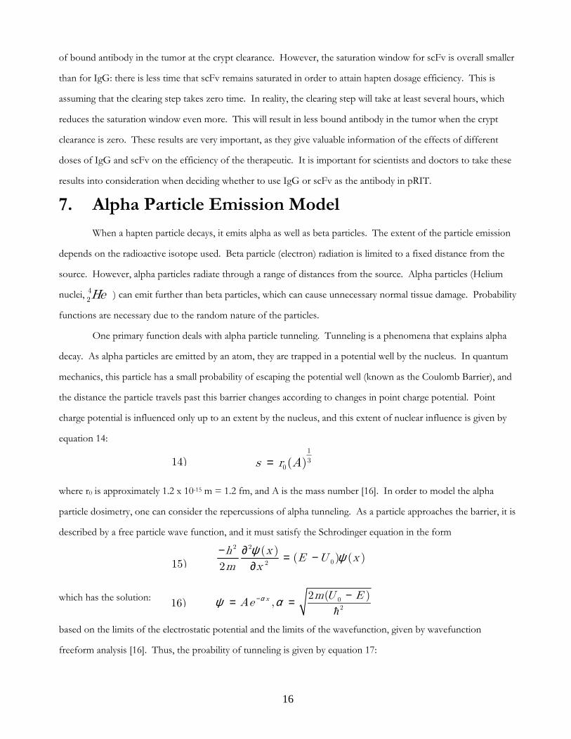
7. Alpha Particle Emission Model

When a hapten particle decays, it emits alpha as well as beta particles. The extent of the particle emission

depends on the radioactive isotope used. Beta particle (electron) radiation is limited to a fixed distance from the

source. However, alpha particles radiate through a range of distances from the source. Alpha particles (Helium

nuclei, ) can emit further than beta particles, which can cause unnecessary normal tissue damage. Probability

functions are necessary due to the random nature of the particles.

One primary function deals with alpha particle tunneling. Tunneling is a phenomena that explains alpha

decay. As alpha particles are emitted by an atom, they are trapped in a potential well by the nucleus. In quantum

mechanics, this particle has a small probability of escaping the potential well (known as the Coulomb Barrier), and

the distance the particle travels past this barrier changes according to changes in point charge potential. Point

charge potential is influenced only up to an extent by the nucleus, and this extent of nuclear influence is given by

equation 14:

where r0 is approximately 1.2 x 10-15 m = 1.2 fm, and A is the mass number [16]. In order to model the alpha

particle dosimetry, one can consider the repercussions of alpha tunneling. As a particle approaches the barrier, it is

described by a free particle wave function, and it must satisfy the Schrodinger equation in the form

which has the solution:

based on the limits of the electrostatic potential and the limits of the wavefunction, given by wavefunction

freeform analysis [16]. Thus, the proability of tunneling is given by equation 17:

42He

1

30( )s r A=14)

2 2

02

( )( ) ( )

2

h xE U x

m x

ψ ψ− ∂ = −∂15)

02

2 ( ),x m U E

Ae αψ α− −= =ℏ

16)

17

where M is the mass of the alpha particle and is Planck’s constant [17] . By making some assumptions about

the frequency of the alpha particle striking the barrier, the penetration formula can be used to calculate an effective

nuclear radius for alpha decay. This function can be used to correlate the half-life decay time of the radiation to

the release energy in mega electron volts:

where t 1/2 is the half life in seconds and Qa is the release energy in MeV [17]. The lower limit of the decay would

then be the distance between the barrier and the nucleus. This distance can be derived from equation 19, which is

Coulomb’s barrier:

where k is Coulomb’s constant, is the permittivity of free space (similar to void fraction), q1 and q2 are charges

of interacting particles, and r is the interaction of the radius [16]. In order to find the upper limit of the alpha

decay, it is necessary to consider the potential charge limit, which differs depending on the element. Using these

two functions as benchmarks for the lower limit and the upper limit of the alpha decay radius, this can be

extrapolated into spherical space, where each hapten particle is moving within the spherical tumor region. This

will give a dosimetry rate equation very similar to equation 9:

This is a very rough equation that will need to be changed and tweaked after testing (analogous to pseudo-code of

a computer program) but it describes the basic idea and the logic behind it. The summation is used to account for

the total concentration of all of the hapten particles within the spheroid region, whereas the lower and upper limits

described are initial parameter barriers which can be used to constrain the rate function. In order to use these

constraints, one must know more about the derivation of the rate equation, and more research and tests are

necessary in order to integrate these constraints into the equation. The void fraction is used to account for the fact

that not all of the tumor is accessible to the hapten particles (it is not a hollow sphere). In order to verify this

equation, a model can be built using tools provided in math software to compute the dose rates and compare the

results to those of both the beta emission model and experiments. Because of the correlation between half-life

decay time and the release energy, measurements of the half-life can be taken in an experimental environment and

1

2

1

2

24

( )

MBR B

QP t e α

π − − − =

ℏ17)

1 2

0

1

4coul

q qU

rπε=19)

20)

( )22

0 2

0 0 0 ( )

( , ) ( , ) sin( )4

coul

UpperLimit TheoreticalrAv

LowerLimit U

F ED r P s A e s ds d d

q

π πλτ ατ τ φ θ φ

π− ⋅= ⋅ ∫ ∫ ∫

1/2loga

t bQα

= +18)

ℏ

0ε

18

can then be used in the equation to solve for the probability values and the dosimetry rates, testing the validity of

the model. This model can then be integrated into the beta emission model to create a full cohesive simulation;

improving this model and integration is the next step in this project and is definitely a future study.

8. Conclusions

Pre-targeted radioimmunotherapy is a promising new treatment for various forms of cancer. With the

focus on treating colorectal cancer, it has become ever more important to model the interactions between

antibodies and antigens and the effects of pRIT on normal body tissue. The colon model developed is a step

towards recreating the entire process of pRIT and studying its effects on the full human body. Tests were run with

the initial tumor spheroid model in order to determine the minimum antibody concentration dosage in order to

attain a full saturation of antibodies in the tumor for both IgG and scFv antibody formats. Tests were also run to

determine the optimum time to dose hapten and run the clearing step at the maximum saturation point. With this

data, the colon model was developed to model each individual cell as they migrated from the crypts into the villi,

with the equations calculating the change in concentrations of antibodies, antigens, and antibody/antigen

complexes at each cell step. The result is a dynamic model that effectively portrays the changes in the

concentrations in the colon. Comparisons were made between the rates of change of concentration in the crypt,

villi, and the tumor, and conclusions were reached that because the concentration of bound antibodies reached

zero at a sufficient time in the colon, hapten could be dosed to the tumor to the effect of a maximum 72%

efficiency (with scFv). This prevents the death of vital stem cells that replenish the digestive lining.

There are many future studies that can be done in order to add to this model. Eventual goals include

incorporating the action of alpha-emitting nuclides in order to observe the toxicity and its effect on the killing of

cells. A stochastic approach can be taken to model alpha emission, because the distance a particle is emitted varies

randomly over time; this theoretical, improved model can be implemented into a full simulation involving

dosimetry calculations. A final study includes modeling the nonspecific toxicity in the human body in order to

plan strategies to limit damage to other vital organs by radiation, such as the kidneys and bone marrow. The

eventual goal is to integrate these three models into one cohesive simulation that will portray the effects of

bispecific targeting of antibodies on various body tissues to and the potency of this treatment against cancer tissue.

9. References

[1] Gregory P Adams, Louis M Weiner. Monoclonal antibody therapy of cancer. Nature Biotechnology 23 (2005),

no. 9, 1147—1157.

19

[2] BBC News Co. Drug Trial Victim’s “Hell Months”. BBC News/Health online. Available at

http://news.bbc.co.uk/2/low/health/5121824.stm (2006/6/27).

[3] Jean-François Beaulieu. Differential expression of the VLA family of integrins along the crypt-villus axis in the

human small intestine. Journal of Cell Science 102 (1992), 427—436.

[4] H. Oliver Brown, Milton L. Levine, Martin Lipkin. Inhibition of intestinal epithelial cell renewal and migration

induced by starvation. American Journal of Physiology 205 (1963), no. 5, 868—872

[5] Rufus M. Clarke. A new method of measuring the rate of shedding of epithelial cells from the intestinal villus of

the rat. Journal of Anatomy, London 11 (1970), 1015—1019.

[6] William M. Deen. Analysis of Transport Phenomena. Oxford University Press: New York (1998).

[7] Ming Z. Fan, James C. Matthews, Nadege M.P. Etienne, Barbara Stoll, Dale Lackeyram. Expression of Apical

L-glutamate transporters in Neotonal Porcine Epithelial Cells Along the Small-Intestinal Crypt-Villus Axis.

American Journal of Physiology 287 (2004) 384-398.

[8] Christilyn P. Graff, K. Dane Wittrup. Theoretical Analysis of Antibody Targeting of Tumor Spheroids:

Importance of Dosage for Penetration, and Affinity for Retention. Cancer Research 63 (2003), 1288--1296

[9] RK Jain. Transport of Molecules, Particles, and Cells in Solid Tumors. Annu Rev Biomedical Engineering

(1999), no. 1, 241--263.

[10] H. Quastler, F.G. Sherman. Cell Population Kinetics in the Intestinal Epithelium of the Mouse. Experimental

Cell Research 17 (1958), 420--438.

[11] George Sgouros. Bone Marrow Dosimetry for Radioimmunotherapy: Theoretical Conditions. The Journal of

Nuclear Medicine 34 (1993), no. 4, 689—694.

[12] Greg M. Thurber, Stefan C. Zajic, K. Dane Wittrup. Theoretic Criteria for Antibody Penetration into Solid

Tumors and Micrometastases. Journal of Nuclear Medicine (2006).

[13] Vermont Cancer Centre Cytometry guidelines: Antibody Concentration. Cytometry User Guideline. (2006)

[14] Jeffrey L. Winkelhake. Effects of Chemical Modification of Antibodies on Their Clearance from the

Circulation. Journal of Biological Chemistry 252 (1976), no. 6, 1865-1868.

[15] K. Dane Wittrup, Bruce Tidor. “Noncovalent Binding Interactions”. Biological Kinetics. (2006).

[16] Author Unknown, “Compendium of Theories of Quantum Mechanics (Collection of concepts)”. Hyperphysics

online. Available at http://230nsc1.phy-astr.gsu.edu/hbase/nuclear/alpdec.html.

[17] Author Unknown, “Radioactivity”, Britannica Online Article, Available at

http://www.britannica.com/nobelprize/article-48295.