Embed Size (px)
Citation preview
A Novel Design Methodology For EnhancedCompressor Performance Based on a Dynamic
Stability Metric
by
Juan Carlos Castiella Ruiz de Velasco
B. Ing. Ingenieria Industrial, Universidad de Navarra (2001)
Submitted to the Department of Aeronautics and Astronautics inpartial fulfilment of the requirements for the degree of
MASTER OF SCIENCE IN AERONAUTICS AND ASTRONAUTICS
at the
MASSACHUSETTS INSTITUTE OF TECHNOLOGY
January 2005
C 2005 Juan C. Castiella Ruiz de Velasco. All rights reserved.
The author hereby grants to MIT permission to reproduce and distribute publicly paper and electronic copies of thisthesis document in whole or in part, and to grant others the right to do so.
Author
Certified by
Department of Aeronautics and AstronauticsJanuary 28, 2005
Pr sso Lonan p vszkyC.R. Soderberg Assistant Profess r of Aero au cp and A onautics
unervisor
Accepted by
MASSACHUSETTS INSTitUTEOF TECHNOLOGY
FEB 10 2005
t ..!BRARIES
y , jaime reraireProfess r of eronautics and Astronautics
Chair, Co ttee on Graduate Students
AEROi

2
A Novel Design Methodology For EnhancedCompressor Performance Based on a Dynamic
Stability Metric
byJuan Carlos Castiella Ruiz de Velasco
Submitted to the Department of Aeronautics and Astronautics inJanuary 28, 2005, in partial fulfilment of the requirements for the
degree of Master of Science in Aeronautics and Astronautics
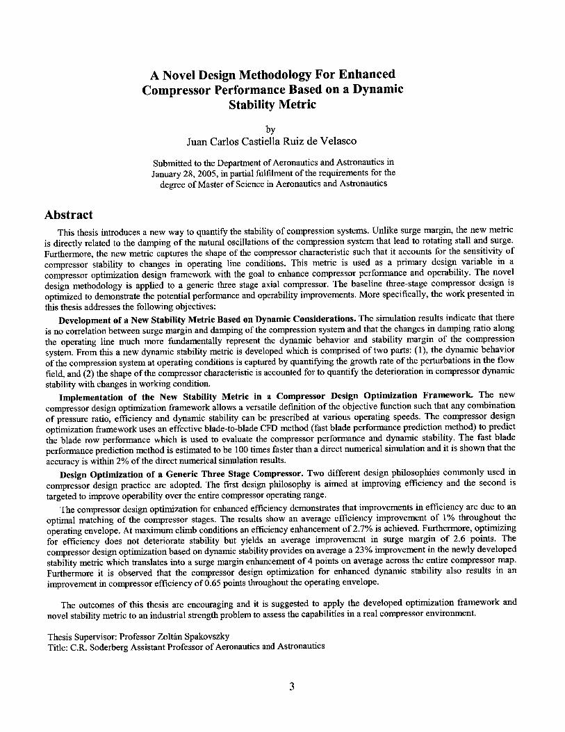
AbstractThis thesis introduces a new way to quantify the stability of compression systems. Unlike surge margin, the new metric
is directly related to the damping of the natural oscillations of the compression system that lead to rotating stall and surge.
Furthermore, the new metric captures the shape of the compressor characteristic such that it accounts for the sensitivity of
compressor stability to changes in operating line conditions. This metric is used as a primary design variable in a
compressor optimization design framework with the goal to enhance compressor performance and operability. The novel
design methodology is applied to a generic three stage axial compressor. The baseline three-stage compressor design is
optimized to demonstrate the potential performance and operability improvements. More specifically, the work presented in
this thesis addresses the following objectives:
Development of a New Stability Metric Based on Dynamic Considerations. The simulation results indicate that there
is no correlation between surge margin and damping of the compression system and that the changes in damping ratio along
the operating line much more fundamentally represent the dynamic behavior and stability margin of the compression
system. From this a new dynamic stability metric is developed which is comprised of two parts: (1), the dynamic behavior
of the compression system at operating conditions is captured by quantifying the growth rate of the perturbations in the flow
field, and (2) the shape of the compressor characteristic is accounted for to quantify the deterioration in compressor dynamic
stability with changes in working condition.
Implementation of the New Stability Metric in a Compressor Design Optimization Framework. The new
compressor design optimization framework allows a versatile definition of the objective function such that any combination
of pressure ratio, efficiency and dynamic stability can be prescribed at various operating speeds. The compressor design
optimization framework uses an effective blade-to-blade CFD method (fast blade performance prediction method) to predict
the blade row performance which is used to evaluate the compressor performance and dynamic stability. The fast blade
performance prediction method is estimated to be 100 times faster than a direct numerical simulation and it is shown that the
accuracy is within 2% of the direct numerical simulation results.
Design Optimization of a Generic Three Stage Compressor. Two different design philosophies commonly used in
compressor design practice are adopted. The first design philosophy is aimed at improving efficiency and the second is
targeted to improve operability over the entire compressor operating range.
The compressor design optimization for enhanced efficiency demonstrates that improvements in efficiency are due to an
optimal matching of the compressor stages. The results show an average efficiency improvement of 1% throughout the
operating envelope. At maximum climb conditions an efficiency enhancement of 2.7% is achieved. Furthermore, optimizing
for efficiency does not deteriorate stability but yields an average improvement in surge margin of 2.6 points. The
compressor design optimization based on dynamic stability provides on average a 23% improvement in the newly developed
stability metric which translates into a surge margin enhancement of 4 points on average across the entire compressor map.
Furthermore it is observed that the compressor design optimization for enhanced dynamic stability also results in an
improvement in compressor efficiency of 0.65 points throughout the operating envelope.
The outcomes of this thesis are encouraging and it is suggested to apply the developed optimization framework and
novel stability metric to an industrial strength problem to assess the capabilities in a real compressor environment.
Thesis Supervisor: Professor Zoltin SpakovszkyTitle: C.R. Soderberg Assistant Professor of Aeronautics and Astronautics
3


Acknowledgments
I first wish to thank Professor Spakovszky for his systematic dedication and for
the continuous support and encouragement he has provided throughout my stay at MIT.
I am particularly thankful for his constructive critical look at my work and effective
counseling leading to a greater learning experience.
I must also thanks my office-mates, Vai-Man, Bobby and Nate for sharing their
experience at GTL with me and for the many conversations we had over the last year
and a half.
I also would like to thanks my roommates, Vince and John for introducing me to
the Canadian way of life and most of all for their friendship that I am sure will endure
over the years to come.
Finally, my last thanks go to my family and Andrea, whose unconditional
support and visits have been essential to the overall success of my stay at MIT.
5

6
Contents
A BSTR A C T .......................................................................................................................................----.. 3
A C K N O W LED G M EN TS ....................................................................................................................... 5
C O N TEN TS.......................................................................................................................................----.. 7
LIST O F FIG U RE S ............................................................................................................................... 11
LIST O F TA BLES ................................................................................................................................. 15
LIST O F TA BLES................................................................................................................................- 15
N O M EN C LA TU RE ............................................................................................................................... 17
IN TR O D U C TIO N................................................................................................................................- 21
1.1 TECHNICAL BACKGROUND................................................................................................ 22
1.1.1 Compressor Stability ................................................................................................ 22
1.1.1.1 Static stability..................................................................................................................... 23
1.1.1.2 Dynamic stability .......................................................................................................... 24
1.1.2 Previous W ork............................................................................................................... 25
1.1.2.1 Current stability metrics..................................................................................................... 26
1.1.3 Off-Design Performance of Multi-Stage Compressors .............................................. 29
1.2 CONCEPTUAL A PPROACH .................................................................................................... 31
1.3 THESIS O RGANIZATION ...................................................................................................... 34
1.4 THESIS OBJECTIVES ........................................................................................................... 34
DEVELOPMENT OF A NEW STABILITY METRIC BASED ON DYNAMIC
C O N SID ER A TIO N S...............................................................................................................................36
2.1 ROTATING STALL INCEPTION PREDICTION MODEL ............................................................ 36
2.2 PREVIOUS DYNAMIC STABILITY CONSIDERATIONS............................................................ 39
2.3 MOTIVATION FOR A NEW SET OF STABILITY METRICS BASED ON DYNAMIC
CONSIDERATIONS.. ............................................................................................................ ............ --- 42
2.4 DEVELOPMENT OF THE NEW STABILITY METRIC ............................................................. 46
2.4.1 Growth rate of theflow fleld perturbations............................................................... 47
2.4.2 Robustness of the compression system stability to changes in operating conditions .... 49
2.4.3 New stability m etric................................................................................................... 50
2.4.4 Example Application of the New Stability Metric ..................................................... 51
7
2.5 SU M M A RY ............................................................................................................................. 54
FAST BLADE PERFORMANCE PREDICTION METHOD........................................................ 55
3.1 M O TIV A TION ......................................................................................................................... 55
3.2 PREVIOUS WORK................................................................................................................... 56
3.3 BLADE PARAMETERIZATION ................................................................................................. 57
3.3.1 Blade Profile Definition ............................................................................................ 58
3.3.2 Effect of Geometric Changes on Blade Performance................................................. 61
3.3.2.1 Stagger Angle Effect on Blade Performance.................................................................. 61
3.3.2.2 Camber Angle Effect on Blade Performance .................................................................. 63
3.3.2.3 Effect of Solidity on Blade Performance......................................................................... 65
3.3.2.4 Effects of Chord on Blade Performance......................................................................... 66
3.4 BLADE PERFORMANCE PREDICTION METHOD.................................................................... 67
3.4.1 B lade F am ily ................................................................................................................. 6 7
3.4.2 Automated CFD utility .................................................................................................. 68
3.4.3 Interpolation Method................................................................................................. 69
3.4.4 Resolution of the blade performance prediction method........................................... 69
COMPRESSOR DESIGN OPTIMIZATION OF A GENERIC 3 STAGE COMPRESSOR ......... 73
4.1 P REVIOU S W O RK ................................................................................................................... 73
4.2 NOVEL COMPRESSOR DESIGN OPTIMIZATION FRAMEWORK .............................................. 74
4.2.1 Compressor Flow field Simulation Code ................................................................... 75
4.2.2 Fast Blade Performance Prediction Method............................................................. 76
4.2.3 O p tim izer....................................................................................................................... 77
4 .2 .3.1 A lgorithm ........................................................................................................................... 77
4.2.3.2 Objective Function Used in the Compressor Design Optimization................................. 78
4.2.3.3 Constraints of the Compressor Design Optimization..................................................... 78
4.2.3.4 Independent Variables of the Compressor Design Optimization ................................... 79
4.3 BASELINE 3 STAGE COMPRESSOR ...................................................................................... 79
4.4 3-STAGE COMPRESSOR DESIGN OPTIMIZATION FOR MAXIMUM EFFICIENCY........................ 82
4.4.1 Objective Function and Constraints.......................................................................... 82
4.4.2 Optimization Results for Maximum Efficiency.......................................................... 83
4.4.3 Design Implications for Maximum Efficiency ............................................................ 85
4.4.4 Effects of Operating Line Constraints on Optimization Results................................. 88
4.5 OPTIMIZATION FOR MAXIMUM STABILITY ......................................................................... 90
4.5.1 Objectives Functions and Constraints........................................................................ 90
4.5.2 Optimization Results for Maximum Stability............................................................. 91
4.5.3 Design Implications for Maximum Stability............................................................... 93
4.6 SUM M A RY ............................................................................................................................. 98
8
SUMMARY AND CONCLUSIONS .................................................................................................. 100
5.1 ASSESSMENT OF THE SHORTCOMINGS OF SURGE MARGIN.................................................. 100
5.2 DEVELOPMENT OF A NEW STABILITY METRIC BASED ON DYNAMIC CONSIDERATIONS...... 101
5.3 IMPLEMENTATION OF THE NEW STABILITY METRIC IN A COMPRESSOR DESIGN OPTIMIZATION
FRAM EW O RK ....................................................................................................................................... 102
5.4 APPLICATION OF THE COMPRESSOR DESIGN OPTIMIZATION FRAMEWORK TO A GENERIC
THREE STAGE COM PRESSOR ................................................................................................................ 102
5.5 DEMONSTRATION OF PERFORMANCE AND OPERABILITY ENHANCEMENTS USING THE NOVEL
COMPRESSOR DESIGN M ETHODOLOGY................................................................................................ 103
5.6 RECOMMENDATIONS FOR FUTURE W ORK ........................................................................... 104
APPENDIX A ....................................................................................................................................... 106
DESCRIPTION OF BLADE ROW LOSSES AND DYNAMICS ................................................... 106
A .I L O SSES................................................................................................................................ 106
A.2 ROTOR/STATOR TRANSMISSION M ATRICES ........................................................................ 108
BIBLIOGRAPHY ................................................................................................................................ 111
9

10
List of Figures
Figure 1-1. Two types of compressor instability phenomena: surge (left) and rotating
stall (right). ............................................................................................................. 23
Figure 1-2. Static Stability- Statically unstable operating point B. ............................ 23
..................... ............................................................................................................ 2 7
Figure 1-3. Compressor and efficiency maps illustrating the definition of surge
m argin ................................................................................................................... 2 7
Figure 1-4. Compressor map for a generic compressor with SMIdustry= 2 5% throughout
the operating envelope........................................................................................ 28
Figure 1-5. Surge margin as defined by NASA and industry and growth rates of the
perturbations in the flow field for the operating points defined in Figure 1-4. ...... 28
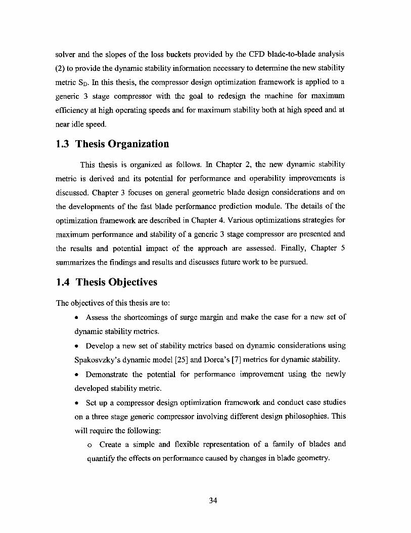
Figure 1-6. Compressor map, gas flow path and non-dimensional velocity triangles of a
generic com pressor. ............................................................................................ 30
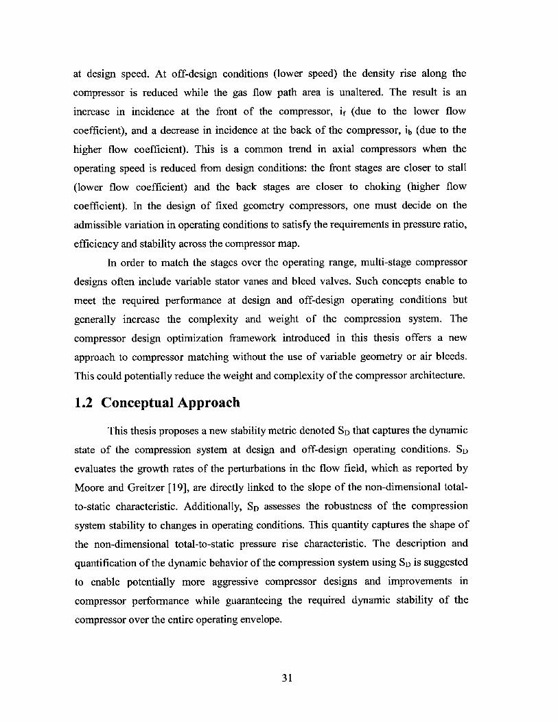
Figure 1-7. Potential for performance improvement while maintaining the required
level of system dam ping ......................................................................................... 32
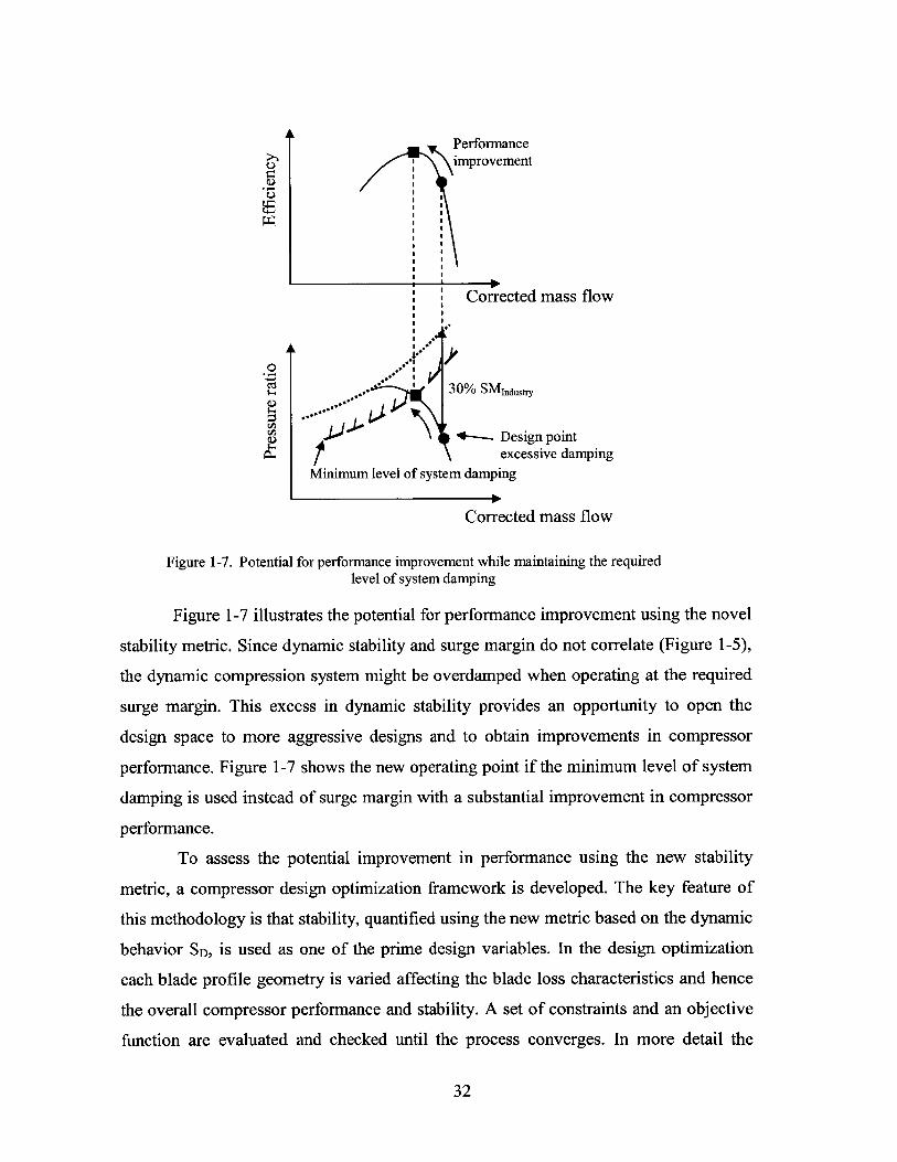
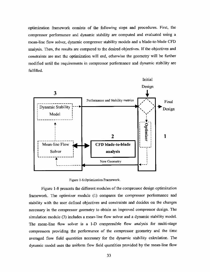
Figure 1-8. Optimization Framework. ....................................................................... 33
Figure 2-1. Modular design compressor model framework (3-stage compressor
ex am ple) ................................................................................................................. 37
Figure 2-2. Equivalent curvature relationship and related preliminary design
m ethodology ........................................................................................................ 40
Figure 2-3. Analogy between compressor dynamics and 1D mass-spring-damper-
oscillator ................................................................................................................. 4 1
Figure 2-4. Compressor map for the 3 stage generic compressor with operating line
with constant SMindustry= 2 0%............................................................................. 43
Figure 2-5. Surge margin as defined by industry (solid) and NASA (dashed) at different
operating speeds for the generic 3 stage compressor with compressor map
illustrated in Figure 2-4 ..................................................................................... 44
11
Figure 2-6. Surge margin as defined by industry (solid), and by NASA (dashed), and
growth rate of the perturbations in the flow field (circles) at different speeds....... 45
Figure 2-7. Potential for performance improvement if dynamic stability is
considered ......................................................................................................... 46
Figure 2-8. Mechanical analogue of a gas turbine system (adopted from [13])........ 47
Figure 2-9. Eigenvalue map for the 3 stage compressor illustrating that the 1st harmonic
of the least stable family of eigenvalues is the first mode becoming unstable....... 48
Figure 2-10.Robustness of compressor stability to changes in operating
conditions.......................................................................................................... 49
Figure 2-1 1.Compressor map illustrating two generic compressors with vastly different
characteristics. .................................................................................................... 52
Figure 2 -12 .SD versus SMNASA for the two compressors considered in Figure 2-
10 ........ .................................................................................................................. 5 2
Figure 2-13.Growth rates and robustness for the two compressors considered in Figure
2 -1 1 ........................................................................................................................ 5 3
Figure 3-1. Parameters used to define the airfoil of a new family of blades. ............ 58
Figure 3-2. Generation of a blade profile (bottom left) by adding camber line (top left)
to thickness distribution (middle left) and then staggering and applying blade pitch
to define the final cascade (right). ....................................................................... 59
Figure 3-3. Thickness distribution defined with four parabolas. Two parabolas are used
to define the top distribution (solid and dashed) and the other two for the bottom
distribution (not show n)...................................................................................... 60
Figure 3-4. Minimum Loss versus stagger angle for a representative blade row
geom etry ................................................................................................................. 62
Figure 3-5. Loss buckets a representative blade row geometry for two levels of stagger
angle (7=20* and y=36*)...................................................................................... 63
Figure 3-6. Minimum loss versus camber for a representative blade row geometry with
camber angle varied between P=240 and P=3 4*.......................... . . . . . . . . . . . . . .. . . .. . . . . . 64
Figure 3-7. Loss buckets for a representative blade row for two different camber angles
(<p=24 0 and p=34 0) ............................................................................................... 64
12
Figure 3-8. Effect of solidity on: minimum loss for a representative blade row geometry
with different stagger angle and camber angle (left) and on incidence at minimum
loss for the high stagger and camber angles case (right).................................... 65
Figure 3-9. Effect on minimum losses of changes in chord for a representative blade
row if chord is varied from c=0.03 m to c=O.1 m................................................... 66
Figure 3-10.Diagram showing the different steps necessary to generate one cascade
perform ance file................................................................................................. 68
Figure 3-11 .Prediction of loss versus incidence for a generic three stage compressor
using direct CFD simulations (dashed) and the fast blade performance prediction
m ethod (solid)...................................................................................................... 70
Figure 3-12.Averaged discrepancy in performance and stability between direct CFD
simulations and performance prediction method for the 4 compressors simulated in
th is th esis. ............................................................................................................... 7 1
Figure 4-1. Gas flow path of the 3 stage baseline compressor. .................................. 80
Figure 4-2. Compressor map and efficiency curves for the 3 stage baseline
com pressor.............................................................................................................81
Figure 4-3. Compressor map and efficiency curves for the baseline 3 stage compressor
(dashed) and the compressor optimized for maximum efficiency (solid).......... 83
Figure 4-4. % Improvem ents in efficiency .................................................................... 84
Figure 4-5. Baseline and optimized compressor blade profile configurations (left) and
stagger angle and camber angle (right) for the baseline and optimized
com pressors.. ...................................................................................................... 85
Figure 4-6. Loss buckets for stator 3 for the baseline compressor (dashed) and the
optimized compressor geometry (solid) at different operating speeds. Working line
operating points are marked by circles ............................................................... 87
Figure 4-7. Efficiency improvements for both optimized geometries.......................89
Figure 4-8. New stability metric SD for the baseline compressor design and the two
compressor designs optimized for maximum stability................... 92
Figure 4-9. Blade profiles (top), stagger angle (left) and camber angle (right) for the
baseline compressor design and the two compressor designs optimized for
m axim um stability. ................................................................................................. 93
13

Figure 4-10.Schematic enhancing dynamic stability by increasing through
changes in compressor stages matching (top) or by changing the shape of the blade
row loss characteristic (bottom )......................................................................... 95
Figure 4-11. Loss buckets for stator 3 for the baseline compressor and the
optimized compressor for maximum stability using objective 1........................ 96
Figure 4-12.Loss buckets for stator 3 for the optimized compressor for maximum
stability using objectives 1 and 2........................................................................ 97
14
List of Tables
Table 3-1. Recommended ranges of geometric parameters to define the blade
fam ily .................................................................................................................... 67
Table 4-1. Variations in incidence, Mach number, stagger angle and unstaggered inlet
metal angle considered in the blade performance database............................... 76
Table 4-2. Incidences into the different blade rows throughout the operating envelope
for the baseline com pressor. .............................................................................. 80
Table 4-3. Performance and stability results of the baseline 3 stage compressor..........81
Table 4-4. Operating line constraints used in the optimization for efficiency...........83
Table 4-5. Results of the compressor design optimization for maximum efficiency.... 84
Table 4-6. Relative Mach number into the individual blade rows for the baseline and
the optim ized com pressors. ................................................................................ 85
Table 4-7. Two test cases, one with tight constraints on the operating line and the other
with an unconstrained operating line................................................................. 88
Table 4-8. Operating line constraints and operating line shift from baseline pressure
ratio values for the two operating line schedules studied................................... 89
Table 4-9. Results of the two compressor design optimizations for maximum
stab ility .... .............................................................................................................. 9 1
15

16

Nomenclature
Acronyms
CFD Computational Fluid Dynamics
DEB Disturbance-Energy Balance
DF Diffusion Factor
GTL Gas Turbine Laboratory
IC initial conditions
MG Moore-Greitzer
MIT Massachusetts Institute of Technology
NS Neutral Stability
PR Pressure Ratio
SM Surge Margin
SM Stall Margin
SQP Sequential Quadratic Programming
Greek
a absolute flow angle
#8 relative flow angle
A difference (when used as a prefix)
( deviation angle, perturbation, damping
j damping ratio, weighting factor
# flow coefficient
y stagger angle
X unstaggered metal angle
(p camber angle
T1 adiabatic efficiency
A blade passage inertia
pU stator blade-row inertia
p air density
Q rotational speed
Oan growth rate
17
to blade row loss coefficient, frequency
aA- rotation rate
F pressure rise coefficient
Ir unsteady-losse time lag
Roman
a speed of sound
A cross-sectional area
B transmission matrix
ce specific heat at constant pressure
c blade-row chord, polynomial interpolation coefficients
i index, incidence
j index, j= j
k, throttle coefficient
L loss coefficient
m mass
th mass flow
M Mach number, number of discrete points along the characteristic
n harmonic number
N rotation speed, number of stages
P pressure
p weighting factor
Q amplification factor
r radius
R mean radius, stage reaction
Re Reynolds number
s eigenvalue, Laplace variable, blade pitch
T temperature
U wheel speed
V non-dimensional velocity
X transmission matrix
Y transmission matrix
Superscripts
18

Ts total-to-static
mean quantity
in relative frame
Subscripts
I inlet or upstream
2 outlet or downstream
AVE averaged value
Cor- corrected value
des at design
dist distribution
initial
line line
NS at neutral stability
noaw reference value
OP at the operating point
0 in tangential direction
R rotor
speed speed
s stator
Sys system
x in axial direction
T stagnation quantity
19

20
Chapter 1
Introduction
Compressor design is an ever growing discipline driven by the desire of
producing safer, cleaner and cheaper engines. Over the past four decades, aerodynamic
research programs have focused on efficiency to reduce operating costs. In the late
nineties, Greitzer and Wisler [11] showed that the potential for cost reduction obtained
from further improvements in efficiency was low and recommended new research areas
with further cost reduction opportunities. Since then, the aero-engine industry has
engaged in some of these research areas, mainly related to the affordability and
operability of compressors. Current research efforts concentrate on the manufacturing
of simpler, fewer parts, and lighter, higher thrust-to-weight engines. Also more recently
a new research direction was launched that focuses on the improvement of the
robustness of the design to manufacturing variabilities, noise reduction and operation
free from instabilities (Garzon [10], Lamb [15], Sidwell [22]).
In order to ensure the safe and stable functioning of the engines throughout the
operating envelope the compressor design must be robust to inlet distortion, compressor
deterioration, foreign object ingestion and acceleration transients. In order to satisfy the
design requirements set by the customer the compressor design is achieved iteratively
with the goal to meet stability, pressure ratio and efficiency targets across the
compressor map. Each iteration is composed of two design phases. The first phase uses
vector diagram design to determine the compressor annulus shape and the radial
distribution of velocity and flow angles along the compressor. The second phase defines
the blade profiles necessary to achieve the desired velocity and pressure distributions.
Upon completion of the two design phases, the performance, pressure ratio and stability
of the compressor are evaluated. While maximum values of efficiency and pressure
21
ratio are desired a minimum amount of stability margin must be met. Generally,
changes to the initial compressor architecture are necessary and the iterative process is
conducted until the final optimal compressor design is obtained (Smith [24]).
Currently the stability of the compressor is measured using a steady-state
stability metric known as surge margin. Surge margin does not assess the dynamic state
of the compression system limiting its performance. This thesis proposes a new stability
metric, SD, based on the dynamic behavior of the compression system. SD, as opposed
to surge margin, captures the dynamic state of the flow field inside the compressor at
operating conditions and the deterioration of dynamic stability with changes in
operating conditions. The knowledge of the dynamic behavior of the compression
system captured in SD is suggested to be used to achieve more aggressive compressor
designs and to obtain improvements in performance while guaranteeing the required
levels of operability. The potential for performance improvement can be maximized if
SD is introduced as a prime design variable in the iterative compressor design
optimization. The outcome of such methodology could yield compressor designs with
enhanced efficiency, pressure ratio and operability.
1.1 Technical Background
Gas turbines produce shaft power or thrust over a range of operating speeds.
Ensuring that this occurs demands a certain pressure rise and efficiency from the
compressor to fulfill the turbine demands and complete the thermodynamic cycle.
Further, gas turbines must be able to run free of instabilities over the entire operating
envelope. While pressure ratio and efficiency can be estimated relatively accurately
during the preliminary design phase, the prediction of instability remains a challenge
and thus has been the focus of much research in the past.
1.1.1 Compressor Stability
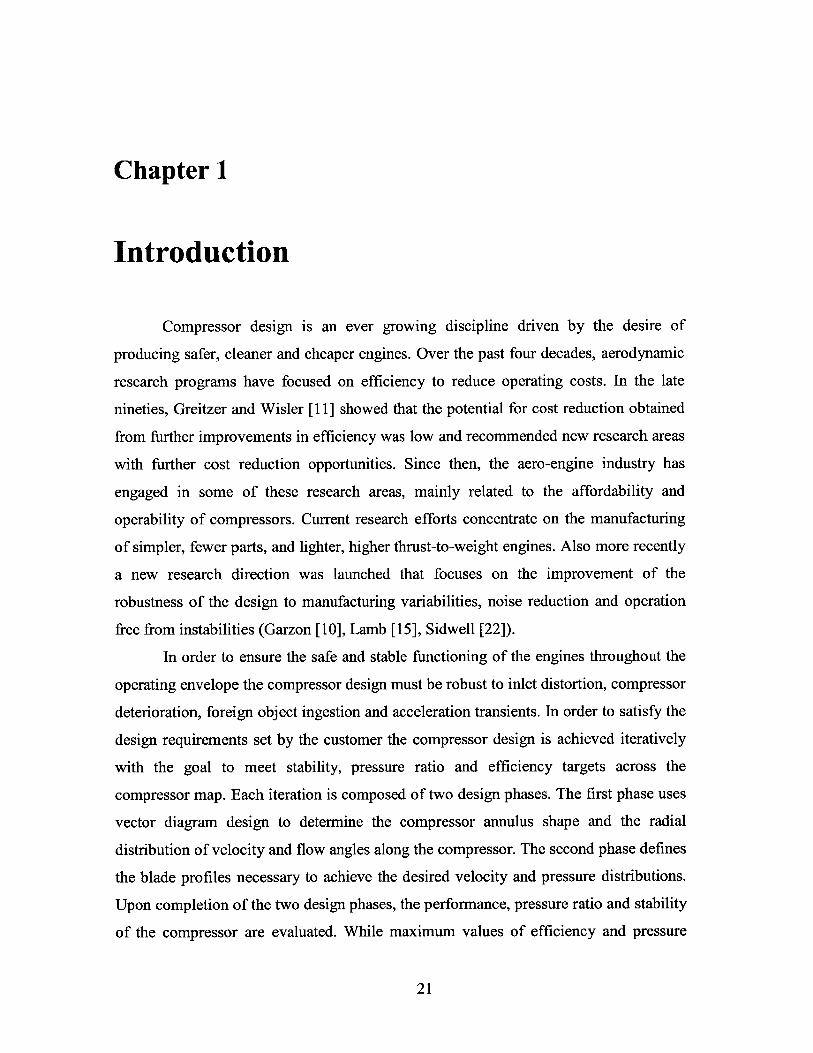
Compression systems present two major types of large scale instabilities, surge
and rotating stall. Surge is an engine wide phenomenon where the annulus averaged
mass flow oscillates with time (3-10Hz) as illustrated in Figure 1-1 on the left. On the
other hand, during rotating stall the annulus averaged mass flow remains more or less
22
constant but the local mass flow varies with time as rotating wave structures travel in
the circumferential direction (20-50Hz) as shown in Figure 1-1 on the right.
Investigating the inception mechanisms of these instabilities is important because surge
and rotating stall limit the performance and the stable range of the compressor.
t I ~ CompressorPlanar RotatingWaves Wave
Structure
Figure 1-1. Two types of compressor instability phenomena: surge (left) and rotating stall (right).
1.1.1.1 Static stability
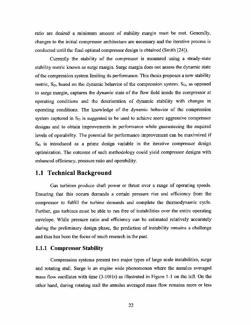
There are two criteria to assess the stability of a compressor. The first criterion
refers to static stability and is formulated in [13]: Static stability requires that the slope
of the throttle line be always larger than the slope of the compressor characteristic.
Turbine throttle lines
Pressure A
Ratio /ACompressor
B X characteristic
Corrected Flow
Figure 1-2.Static Stability- Statically unstable operating point B.
23
Figure 1-2 illustrates the static stability criterion. Suppose that the compressor is
operating at point A. A sudden deficit in compressor mass flow will yield a higher
pressure rise than that demanded by the turbine. This will accelerate the flow and return
the operating point back to the original point A. If the same sudden mass flow change
occurs at point B, the turbine will demand a higher pressure rise from the compressor
than it can provide. The result is a statically unstable compressor which is associated
with a pure divergence from the initial state B.
1.1.1.2 Dynamic stability
The static stability criterion does not capture the dynamic flow phenomena
taking place inside the compressor and thus is not a sufficient criterion to avoid
instability (Greitzer [13]). The observed instability phenomena in practice are
characterized by a growing oscillatory motion about an initial operating point
manifesting the dynamic nature of these instabilities. If these small amplitude
perturbations of the flow field continue to grow with time, one of the two types of large
scale instabilities, surge and rotating stall, will appear.
Rotating stall appears as a circumferentially non-uniform flow distribution
around the annulus at 20-70% of the rotor speed. McDougall et al. [18] and Day [6]
identified two different inception mechanisms for rotating stall. So called "spikes" are
sudden short length scale disturbances (of the order of one blade pitch) which provoke
flow breakdown causing the compressor stall. The second path into instability, referred
to as modal stall inception (Moore and Greitzer [19]), involves the temporal growth of
larger length scale circumferential perturbations (of the order of the compressor
circumference). As mass flow is decreased rotating stall will be initiated in the form of
spikes if the critical incidence of any of the stages in the compressor is exceeded before
reaching the top of the total to static pressure rise characteristic. Otherwise, flow
breakdown can be initiated by modal stall (Camp and Day [4]).
Surge is an engine wide phenomenon. This large scale instability appears in the
form of circumferentially uniform waves oscillating in the longitudinal direction at low
frequency (5% of rotor speed).
24
This thesis focuses on rotating stall in high-speed axial compressors. The
compressors investigated have relatively high flow coefficients and low loading such
that rotating stall is more likely to be initiated by modal waves. Furthermore the hub-to-
tip radius ratios are high and the incidence into the individual blade rows are such that
the peak of the pressure rise characteristic is reached before the critical incidence is
exceeded (Camp and Day [4]).
1.1.2 Previous Work
Already in the early days of compressor development, achieving sufficient
levels of stability throughout the compressor map was one of the main concerns and
challenges in compressor design. In the early fifties, Lieblein et al. [16] introduced the
diffusion factor. This parameter allows to assess the blade loading near stall. However,
the diffusion factor is not suitable to explain the mechanisms leading to rotating stall
and surge. Up until the eighties, sufficient levels of stability were ensured using stall
prediction methods mostly based on experience and correlations (Smith [24]). Over the
past two decades, the introduction of CFD and a better theoretical understanding of the
processes leading to stall and surge has enabled improved compressor designs with
enhanced operability. In particular, the work by McDougall [18] and Day [6] identifies
two inception mechanisms of stall, "spike" and "modal oscillations". Moore and
Greitzer [19] report a theory to predict the modal stall inception of rotating stall. They
are able to trace the evolution of disturbances in the compressor system and identify the
top of the non-dimensional total-to-static pressure rise characteristic as the limit of
stable compressor operation. Moreover, they show that pure surge and rotating stall
modes can exist without one another but are coupled in general. Longley [17], reviews
the Moore-Greitzer based dynamic compressor modeling and discusses the importance
of further research necessary in the modeling of three-dimensional flow phenomena.
Bonnaure [2], Feulner [8] and Weigl [27] introduce compressibility considerations into
the existing Moore-Greitzer models and Frechette [9] uses the newly gained
understanding of the compressible dynamic stability phenomena to introduce the
concept of disturbance energy. He also suggests that in the compressor design phase a
potential for performance improvement exists if dynamic stability replaces surge
25

margin. This idea opens the door to new design possibilities and constitutes the basis on
which this thesis is built. Dorca [7] further develops the work done by Frechette and
uses the dynamic compressor model developed by Spakovszky [25] and basic dynamic
system modeling to establish a new set of stability metrics. In addition, Dorca
establishes a relation between stable flow range and dynamic stability, referred to as the
Equivalent Curvature Relation. This tool proves to be useful during preliminary
compressor design and helps to establish a first approximation to the compressor
characteristic with the desired dynamic stability, pressure ratio and mass flow.
The stability metrics proposed by Dorca [7] seem to be limited for application to
industrial compressor design and are discussed in Chapter 2. Particularly, the
disturbance energy approach is computationally expensive and the equivalent curvature
relation does not account for general variations in shape of the compressor
characteristic.
More recently, Perrot [22] reports the implementation of a compressor design
optimization framework using surge margin as the prime design variable. He
demonstrates a 6% improvement in surge margin of a 3 stage compressor at design
conditions at the cost of a 0.5% drop in efficiency and a 2% decrease in pressure ratio.
The research in this thesis builds on the work by Frechette [9], Dorca [7], and
Perrot [22] and addresses their shortcomings by introducing a new stability metric based
on dynamic considerations coupled with a compressor design optimization framework.
1.1.2.1 Current stability metrics
Ideally, one would like to obtain the maximum possible compressor efficiency
and pressure ratio. In practice however, the operating points must be kept at a "safe"
distance from the limit of stable compressor operation. This limit is referred to as the
surge line. A certain amount of surge margin must be guaranteed (usually about 20-
30%) to ensure that the operating condition will remain in the stable operating region
throughout the operating envelope and in the presence of inlet flow distortion, engine
deterioration or acceleration transients.
26
A
.o Surge line.
Limit to stable regimp..-7 -
.SM as.defined by
SM as industrydefinedby Nasa
x Maximum pressure ratio operating point* Design operating point at required SMM Maximum efficiency operating point
Corrected mass flow Corrected mass flow
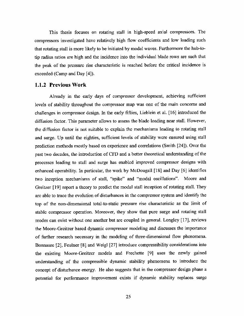
Figure 1-3. Compressor and efficiency maps illustrating the definition of surge margin
The amount of surge margin or distance between the operating point and the
surge point in the compressor map is commonly quantified using two different
definitions. Figure 1-3 illustrates both definitions of surge margin. Surge margin as
commonly defined in industry evaluates the distance between the operating point and
the surge point at constant corrected mass flow. On the other hand, surge margin as
defined by NASA measures the distance between the operating point and the surge
point at constant corrected speed. The NASA definition of surge margin accounts for
throttle area changes representing the equivalent throttling process required to take the
compressor into stall (Cumpsty [5]). Figure 1-3 also illustrates that the demands in
surge margin limit the maximum possible compressor performance in pressure ratio and
efficiency. It is evident from the schematic that operating points of maximum pressure
ratio, maximum efficiency and minimum surge margin do not coincide. Thus
performance must sometimes be compromised with operability in the compressor
design.
27
kL
3
1.5
Ia. 2
0.5
100%
90%80%
70%
Corrected Mass Flow
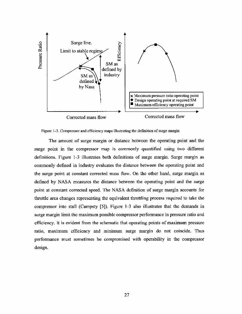
Figure 1-4. Compressor map for a generic compressor withSMIndusr= 2 5% throughout the operating envelope.
Figure 1-4 illustrates the compressor map for a generic 3 stage compressor with
an operating line fixed such that the surge margin as defined in industry is 25%
throughout the operating envelope. In order to assess if the two definitions of surge
margin represent the same operability trends their values are calculated across the
operating envelope.
50.00 60.00 70.00 80.00
% Corrected Speed
90.00
0.00
-1.00
-2.00
-3.000
-4.00 L
-5.00-. -0
-6.00
-7.00
-8.00100.00
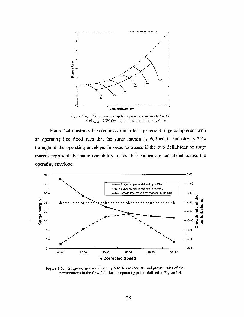
Figure 1-5. Surge margin as defined by NASA and industry and growth rates of theperturbations in the flow field for the operating points defined in Figure 1-4.
28
40
35
301
25-
E 20--0
= 15--
10--
5-
0-
---- Surge margin as defined by NASA
- -A- - Surge Margin as defined in industry
-*- Growth rate of the perturbations in the flow
I I-I
e'O1 1 1 1
0
0L
4.5 1
4
10
-
Figure 1-5 presents the values of the two surge margin definitions at the
operating conditions illustrated in Figure 1-4. Clearly, the two definitions do not
represent the same levels of surge margin since as the value of surge margin as defined
by NASA decreases with increasing speed, the value of surge margin by the industry
definition remains constant. As outlined earlier, the dynamics of the compression
system dominate the compressor stability behavior. A detailed analysis of the dynamics
of the same compression system was conducted using the modeling methodology
outlined later in this thesis. The goal was to identify if any of the two definitions of
surge margin captured the dynamic phenomena taking place in the compressor flow
field. The results show that neither of the two definitions of surge margin capture the
dynamics of the compression system, represented here by the growth rate of the small
amplitude perturbations in the flow field. The limitations to capture the dynamic
stability of the compressor of both definitions of surge margin suggest an opportunity
for a new stability metric based on dynamic considerations. Furthermore, the
incorporation of such a metric in the compressor design phase is conjectured to enable
more aggressive compressor designs enabling improvements in performance while
insuring adequate levels of stability. This thesis is based on existing compressor
stability models (Spakovszky [25]) that have enabled a description of the stability
phenomena and are used to evaluate the new stability metric. The new stability metric is
then used in a compressor design optimization framework to enhance performance and
stability.
1.1.3 Off-Design Performance of Multi-Stage Compressors
Fixed geometry compressors (i.e. low pressure compressors without variable
stator vanes) are designed such that the compressor efficiency is maximized where the
engine operates most of the time, that is generally at the design point (Cumpsty [5]).
However, engines do also operate at off-design conditions which still demand adequate
levels of pressure ratio, efficiency and stability. The operability requirements across the
compressor map might not be achievable with a fixed geometry such that compromises
need to be made, usually with emphasis on stability at low speed and efficiency at
design conditions (Cumpsty [5]).
29

0
L. ' HighLow 'SpeedSpeed
Corrected mass flow Fixed compressor geometry
. Low speed
--- High speed
Front Back
Figure 1-6. Compressor map, gas flow path and non-dimensional velocitytriangles of a generic compressor.
To illustrate the effects of off-design performance and stage matching on blade
row performance consider the following example. The flow coefficient <=Vx/U
determines the incidence and thus, if Mach number effects are ignored, the performance
of the individual blade rows. As operating conditions change, the flow coefficients into
the individual blade rows will depart from their nominal values. This causes some of the
stages to choke and others to stall. This occurrence is illustrated in Figure 1-6 which
shows schematically two speed lines and the corresponding operating points together
with the gas path flow area along the compressor. The pressure rise along the machine,
which is larger at high speeds than at low speeds, leads to an increased density rise at
high speed operation compared to the low speed operation. The fixed gas path
contraction is chosen to achieve the required flow coefficients at design conditions.
Figure 1-6 shows the velocity triangles at the front and the back of the
compressor for low and high speed operation. The velocity triangles at design speed are
the same for the front and the back stages (#Design front Design back) since the area
contraction was designed to accommodate the changes in density along the compressor
30
at design speed. At off-design conditions (lower speed) the density rise along the
compressor is reduced while the gas flow path area is unaltered. The result is an
increase in incidence at the front of the compressor, if (due to the lower flow
coefficient), and a decrease in incidence at the back of the compressor, ib (due to the
higher flow coefficient). This is a common trend in axial compressors when the
operating speed is reduced from design conditions: the front stages are closer to stall
(lower flow coefficient) and the back stages are closer to choking (higher flow
coefficient). In the design of fixed geometry compressors, one must decide on the
admissible variation in operating conditions to satisfy the requirements in pressure ratio,
efficiency and stability across the compressor map.
In order to match the stages over the operating range, multi-stage compressor
designs often include variable stator vanes and bleed valves. Such concepts enable to
meet the required performance at design and off-design operating conditions but
generally increase the complexity and weight of the compression system. The
compressor design optimization framework introduced in this thesis offers a new
approach to compressor matching without the use of variable geometry or air bleeds.
This could potentially reduce the weight and complexity of the compressor architecture.
1.2 Conceptual Approach
This thesis proposes a new stability metric denoted SD that captures the dynamic
state of the compression system at design and off-design operating conditions. SD
evaluates the growth rates of the perturbations in the flow field, which as reported by
Moore and Greitzer [19], are directly linked to the slope of the non-dimensional total-
to-static characteristic. Additionally, SD assesses the robustness of the compression
system stability to changes in operating conditions. This quantity captures the shape of
the non-dimensional total-to-static pressure rise characteristic. The description and
quantification of the dynamic behavior of the compression system using SD is suggested
to enable potentially more aggressive compressor designs and improvements in
compressor performance while guaranteeing the required dynamic stability of the
compressor over the entire operating envelope.
31
LPerformanceimprovement
Corrected mass flow
0
+--Design pointexcessive damping
Mnimum level of system damping
Corrected mass flow
Figure 1-7. Potential for performance improvement while maintaining the requiredlevel of system damping
Figure 1-7 illustrates the potential for performance improvement using the novel
stability metric. Since dynamic stability and surge margin do not correlate (Figure 1-5),
the dynamic compression system might be overdamped when operating at the required
surge margin. This excess in dynamic stability provides an opportunity to open the
design space to more aggressive designs and to obtain improvements in compressor
performance. Figure 1-7 shows the new operating point if the minimum level of system
damping is used instead of surge margin with a substantial improvement in compressor
performance.
To assess the potential improvement in performance using the new stability
metric, a compressor design optimization framework is developed. The key feature of
this methodology is that stability, quantified using the new metric based on the dynamic
behavior SD, is used as one of the prime design variables. In the design optimization
each blade profile geometry is varied affecting the blade loss characteristics and hence
the overall compressor performance and stability. A set of constraints and an objective
function are evaluated and checked until the process converges. In more detail the
32
optimization framework consists of the following steps and procedures. First, the
compressor performance and dynamic stability are computed and evaluated using a
mean-line flow solver, dynamic compressor stability models and a blade-to-blade CFD
analysis. Then, the results are compared to the desired objectives. If the objectives and
constraints are met the optimization will end, otherwise the geometry will be further
modified until the requirements in compressor performance and dynamic stability are
fulfilled.
Initial
Design
3Performance and Stability metrics % Final
Dynamic Stability :- - -
Model- - - - - ------- I
A0
I |
2 1Mean-line Flow CFD blade-to-blade
Solver analysis
New Geometry---------. 4--
Figure 1-8.Optimization Framework.
Figure 1-8 presents the different modules of the compressor design optimization
framework. The optimizer module (1) compares the compressor performance and
stability with the user defined objectives and constraints and decides on the changes
necessary in the compressor geometry to obtain an improved compressor design. The
simulation module (3) includes a mean-line flow solver and a dynamic stability model.
The mean-line flow solver is a 1 -D compressible flow analysis for multi-stage
compressors providing the performance of the compressor geometry and the time
averaged flow field quantities necessary for the dynamic stability calculation. The
dynamic model uses the uniform flow field quantities provided by the mean-line flow
33
solver and the slopes of the loss buckets provided by the CFD blade-to-blade analysis
(2) to provide the dynamic stability information necessary to determine the new stability
metric SD. In this thesis, the compressor design optimization framework is applied to a
generic 3 stage compressor with the goal to redesign the machine for maximum
efficiency at high operating speeds and for maximum stability both at high speed and at
near idle speed.
1.3 Thesis Organization
This thesis is organized as follows. In Chapter 2, the new dynamic stability
metric is derived and its potential for performance and operability improvements is
discussed. Chapter 3 focuses on general geometric blade design considerations and on
the developments of the fast blade performance prediction module. The details of the
optimization framework are described in Chapter 4. Various optimizations strategies for
maximum performance and stability of a generic 3 stage compressor are presented and
the results and potential impact of the approach are assessed. Finally, Chapter 5
summarizes the findings and results and discusses future work to be pursued.
1.4 Thesis Objectives
The objectives of this thesis are to:
e Assess the shortcomings of surge margin and make the case for a new set of
dynamic stability metrics.
* Develop a new set of stability metrics based on dynamic considerations using
Spakosvzky's dynamic model [25] and Dorca's [7] metrics for dynamic stability.
e Demonstrate the potential for performance improvement using the newly
developed stability metric.
* Set up a compressor design optimization framework and conduct case studies
on a three stage generic compressor involving different design philosophies. This
will require the following:
o Create a simple and flexible representation of a family of blades and
quantify the effects on performance caused by changes in blade geometry.
34

o Using blade-to-blade CFD simulations establish an effective link between
blade profile geometry, incidence, Mach number and blade performance.
o Implement the new set of stability metrics and the blade performance
prediction method in a flexible compressor design optimization framework.
* Demonstrate the potential performance and operability improvements of a 3
stage compressor using the novel compressor design optimization framework.
35
Chapter 2
Development of a New Stability MetricBased on Dynamic Considerations
This chapter briefly introduces the existing dynamic compressor model [25]
used throughout this thesis to predict compressor stability. In addition, previous efforts
to develop stability metrics based on dynamic considerations (Dorca [7]) are reviewed.
Then the advantages of dynamic stability compared to surge margin are assessed using
a generic compressor example. Next the potential performance improvements enabled
by dynamic stability considerations are demonstrated. Finally the new stability metric
based on dynamic considerations is defined and the benefits compared to conventional
stability metrics are assessed.
2.1 Rotating Stall Inception Prediction Model
The objective of the dynamic compressor model is to quantify the temporal
evolution of the small perturbations in the flow field to predict the inception of the
larger amplitude non-linear phenomena surge and rotating stall. The Moore-Greitzer
[19] theory establishes that the grow rates of the perturbations in the flow field vary
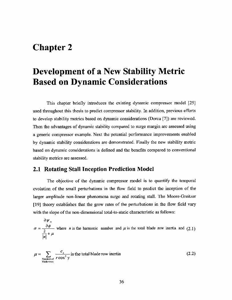
with the slope of the non-dimensional total-to-static characteristic as follows:
aw
- 2 where n is the harmonic number and p is the total blade row inertia and (2.1)
InI+
p is the total blade row inertia (2.2)Numberof r cos yblade rows
36
Consequently, the Moore-Greitzer theory predicts that the compressor becomes
unstable at the top of the non-dimensional total-to-static pressure rise characteristic
(a=O indicates neutral stability) and that the growth rates of the perturbations in the
flow field diminish as the slope of the pressure rise characteristic decreases.
The model used in this thesis is based on an existing modular formulation of the
problem capable of dealing with axial and centrifugal compression systems, rotor-stator
blade row component interactions and unsteady radially swirling flows (Spakovszky
[25]).
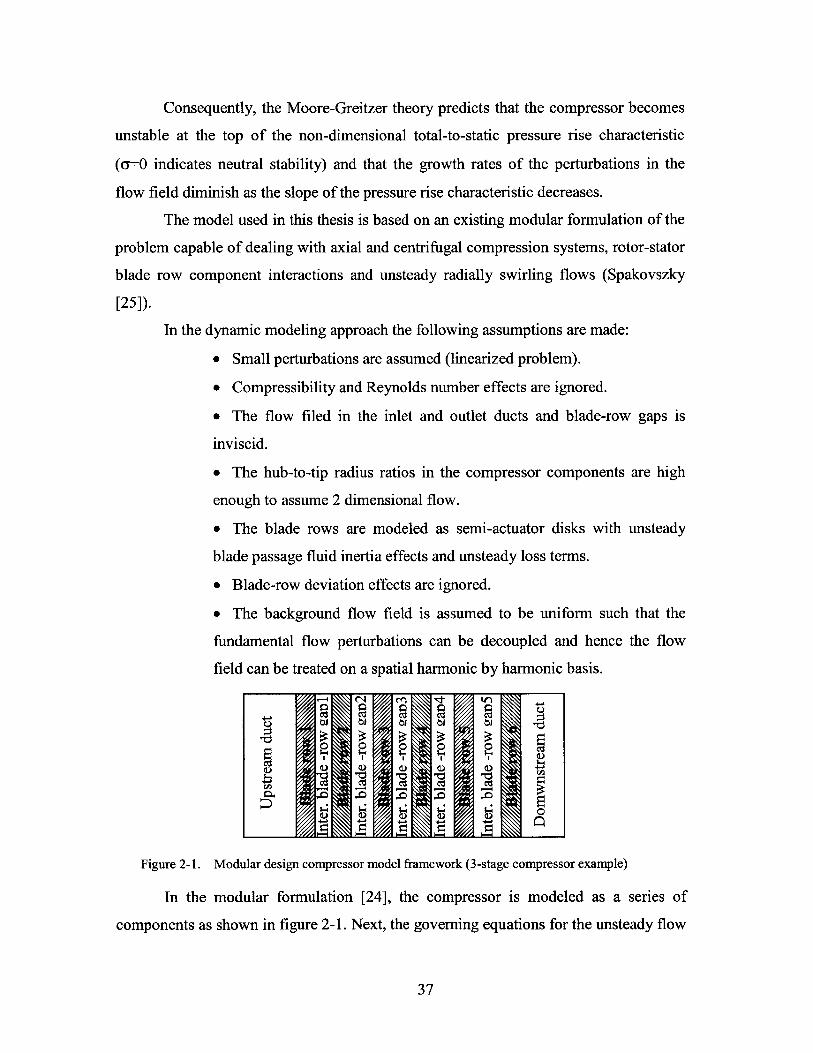
In the dynamic modeling approach the following assumptions are made:
* Small perturbations are assumed (linearized problem).
* Compressibility and Reynolds number effects are ignored.
* The flow filed in the inlet and outlet ducts and blade-row gaps is
inviscid.
* The hub-to-tip radius ratios in the compressor components are high
enough to assume 2 dimensional flow.
* The blade rows are modeled as semi-actuator disks with unsteady
blade passage fluid inertia effects and unsteady loss terms.
" Blade-row deviation effects are ignored.
" The background flow field is assumed to be uniform such that the
fundamental flow perturbations can be decoupled and hence the flow
field can be treated on a spatial harmonic by harmonic basis.
co CIO OW CPO CPO
Figure 2-1. Modular design compressor model framework (3-stage compressor example)
In the modular formulation [24], the compressor is modeled as a series of
components as shown in figure 2-1. Next, the governing equations for the unsteady flow
37
field through each duct or inter blade-row gap and rotor or stator blade row are
linearized in order to solve for the perturbations in pressure, tangential and axial
velocity. The flow field perturbations are written in matrix form in order to obtain the so
called transmission matrices for each of the compression system components (for a
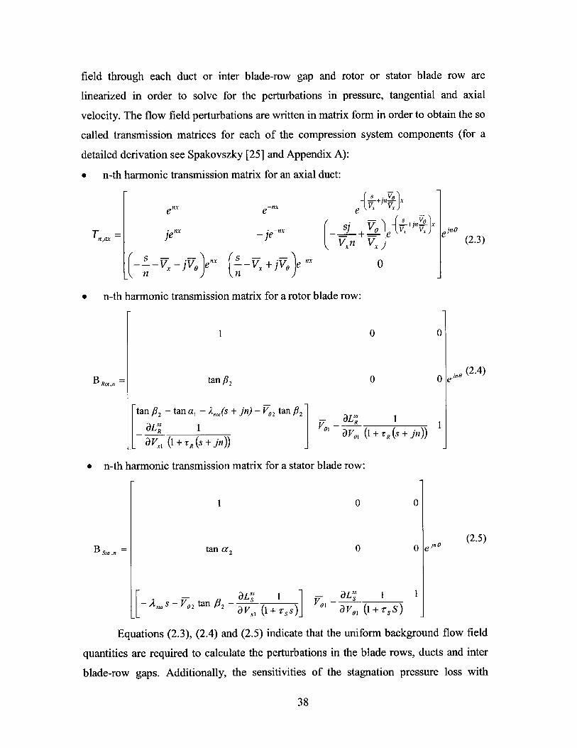
detailed derivation see Spakovszky [25] and Appendix A):
* n-th harmonic transmission matrix for an axial duct:
e nx
je nx
: e~ jv nx- -, jV e"'
e-"x
- jex
S -VX + jv-"n)
-( S S.Ve V )
e +J=J
Vxn )
0
e n-th harmonic transmission matrix for a rotor blade row:
BRot,n =
01
tan fi2 0
tan #2 - tan a, - Ay0 t(s + jn) - V. 2 tan #32 aL"IL "L1 R
R V9 a VO (1 + 'rR (S
aV,,(1 + rR (+j
* n-th harmonic transmission matrix for a stator blade row:
B Sta,n =
1
tan a2
0
0
aL" 1 - L" 1 1-A s -Vo ta -s y _ s
V02 an 42 a Vx, (I+ rss) V, (1+ r 3S)
Equations (2.3), (2.4) and (2.5) indicate that the uniform background flow field
quantities are required to calculate the perturbations in the blade rows, ducts and inter
blade-row gaps. Additionally, the sensitivities of the stagnation pressure loss with
38
Tax = (2.3)
0
(2.4)0 Ie'no
1
0
0(2.5)
e in 0

respect to the non-dimensional axial and tangential velocities, and need to be
calculated in each blade row. As will be demonstrated in Chapter 4, these loss
sensitivities are critical for the overall system stability. The transmission matrices
contain the dynamics of each of the compression system components and can be
stacked together by linking the downstream flow perturbations of one component to the
upstream flow perturbations of the following component. This yields a system wide
transmission matrix which contains the n-th harmonic dynamic information of the
compressor and is in general of the form:
X sysn = T n (X2Nstages +1,1 , s)_ - - [Bstain - Bgap,2i,n -,n
i=2Nstages (2.6)
-Bsta, ,B gap ,2,n -Brotin -Taxn (x1,N int S
with sn=on-j a such that a, and a, are the growth rate and the rotation rate of the n-th
harmonic flow field perturbations.
Specification of the inlet and exit boundary conditions of the overall
compression system at the end of the upstream and downstream ducts leads to the
following eigenvalue problem:
dtEC -XY,0,E 100,I 0 1 0]>S=an-jn(27
det1IC j=0,EC=[1 0 0],IC= 0 0-1j" (2.7)
The solution of the eigenvalue problem yields eigenvalues of the form s=o--jaA
that are used to assess the compression system dynamic stability as will be discussed in
next sections.
2.2 Previous Dynamic Stability Considerations
The physical understanding of the rotating stall and surge inception mechanisms
has been successfully used for active rotating stall and surge control purposes under the
MIT Smart Engine program (Paduano et al. [20]). Beyond the active control
applications, Frechette [9] introduces a dynamic stability analysis based on an energy-
like quantity, the disturbance energy balance (DEB). DEB quantifies the temporal
behavior of the energy of the small perturbations in the flow field. A negative value of
DEB is desired since it indicates that the energy of the perturbations in the flow field is
39
decreasing with time. In addition, Frechette suggests design guidelines to improve
operability based on dynamic stability and energy considerations. He concludes that the
strongest impact on stability occurs if the geometry of the front stages of the compressor
is adjusted. Frechette indicates that the changes required at the front of the compressor
to improve operability must increase the loss and deviation of the airfoil profiles, i.e. by
increasing stagger angle and camber angle, or reducing blockage, i.e. modify 3D
features, and end wall effects. Further, Frechette introduces the concept of blade row
powers. Blade row powers measure the contribution in disturbance energy of the
individual blade rows to the overall compressor disturbance energy. A negative blade
row power indicates that the particular blade row is dissipating the disturbance energy
of the compression system and thus is improving the stability of the compression
system. A positive blade row power implies that the blade row adds energy to the
system.
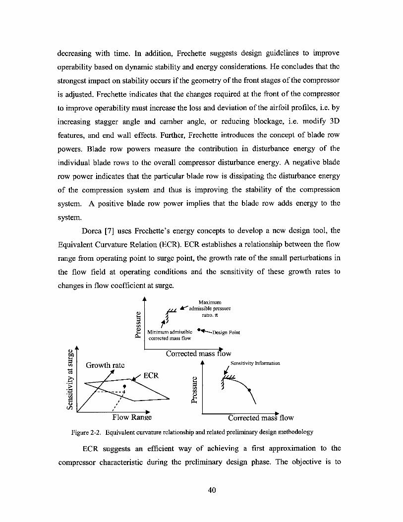
Dorca [7] uses Frechette's energy concepts to develop a new design tool, the
Equivalent Curvature Relation (ECR). ECR establishes a relationship between the flow
range from operating point to surge point, the growth rate of the small perturbations in
the flow field at operating conditions and the sensitivity of these growth rates to
changes in flow coefficient at surge.
MaximumA' admissible pressure
ratio. t
Minimum admissible *'-Design Pointcorrected mass flow
Corrected mass flow
Growth rate Sensitivity Information
ECR
- a)4
Flow Range Corrected mass flow
Figure 2-2. Equivalent curvature relationship and related preliminary design methodology
ECR suggests an efficient way of achieving a first approximation to the
compressor characteristic during the preliminary design phase. The objective is to
40
obtain a compressor characteristic that satisfies the demands in pressure ratio, mass
flow and dynamic stability at design operating conditions and achieves given maximum
pressure ratio and minimum corrected mass flow requirements. These requirements
alone are not enough to obtain a first approximation to the compressor characteristic as
illustrated in Figure 2-2 (top). However, since the flow range between working points
and surge limit and the value of the growth rate of the perturbations are known, ECR
provides the value of the sensitivity of the growth rates of the perturbations to changes
in flow coefficient (see bottom-left figure in Figure 2-2). The sensitivity of the growth
rates of the perturbations to changes in flow coefficient is directly linked to the
curvature of the compressor characteristic. This extra information is used with the initial
requirements to obtain the first approximation to the compressor characteristic. Then,
the iterative optimization process can be initiated with a preliminary compressor design
that satisfies the desired dynamic stability and verifying the main requirements in
pressure ratio and corrected mass flow.
M 244 1- 2
Compressor o _ e(ait))t 1Qflow field vxe - Q= 2o2
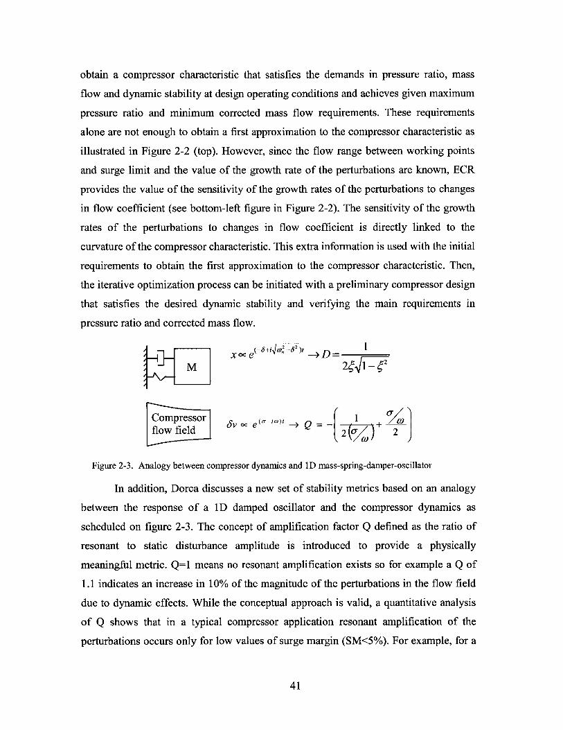
Figure 2-3. Analogy between compressor dynamics and 1D mass-spring-damper-oscillator
In addition, Dorca discusses a new set of stability metrics based on an analogy
between the response of a ID damped oscillator and the compressor dynamics as
scheduled on figure 2-3. The concept of amplification factor Q defined as the ratio of
resonant to static disturbance amplitude is introduced to provide a physically
meaningful metric. Q=1 means no resonant amplification exists so for example a Q of
1.1 indicates an increase in 10% of the magnitude of the perturbations in the flow field
due to dynamic effects. While the conceptual approach is valid, a quantitative analysis
of Q shows that in a typical compressor application resonant amplification of the
perturbations occurs only for low values of surge margin (SM<5%). For example, for a
41

rotation rate of o)=0.2, there is no amplification of the perturbations (Q=1) for values of
growth rate smaller than a<-0.2. At these operating conditions (a=-0.2), the surge
margin values are below 5%. These low values of surge margin at which Q starts to
grow are not suitable for application of this concept to industrial compressor design.
Furthermore the evaluation of DEB is computationally expensive because it
requires the integration of the perturbations in the flow field along the compressor. For
the incompressible dynamic model used in this thesis, the first harmonic of the least
stable family of eigenvalues is in general the first eigenvalue to become unstable. Thus,
considering only the growth rate of this eigenvalue is sufficient to assess the dynamic
stability at a given operating condition. The new stability metric takes advantage of this
statement to simplify the calculations. In addition, the previously developed dynamic
stability metrics do not directly account for general changes in the shape of the
compressor characteristic which is related to the robustness of the dynamic stability of
the compression system to changes in operating conditions. This research also addresses
this shortcoming and proposes a new stability metric based on dynamic considerations.
2.3 Motivation for a New Set of Stability Metrics Based on
Dynamic Considerations
Chapter 1 briefly discussed the importance of meeting the required levels of
dynamic stability throughout the operating envelope to avoid rotating stall and surge.
To set the stage for a new stability metric, a more detailed treatment of the matter
supported by numerical examples is presented in this section.
Currently, stable operation in the presence of inlet distortion, throttle changes
and engine deterioration is achieved using surge margin. Surge margin is commonly
defined in industry as:
SMIndusty = nSurge -nOperating (2.8)KOperating Corrected mass flow
Cumpsty [5] suggests that a more adequate definition of surge margin should
consider the changes in outlet corrected mass flow between the operating line and the
surge line. The advantage of this definition is that it provides a measure of the throttling
42
process necessary to take the compressor into stall. Surge margin as commonly defined
by NASA captures this effect and is defined as:
SMNASA Operating Corr,Surge (2.9)Surge Corr,Operating ) Corrected Speed
Since both definitions of surge margin are used in practice to determine
compressor operability it is useful to compare the two for the same compressor. The
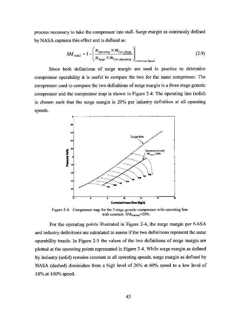
compressor used to compare the two definitions of surge margin is a three stage generic
compressor and the compressor map is shown in Figure 2-4. The operating line (solid)
is chosen such that the surge margin is 20% per industry definition at all operating
speeds.
21-
Surge line
Operating line withSM ,=20%
IA
IA
4 6 a 10 12 14 10
Conrected mass flow(Kg/s)
Figure 2-4. Compressor map for the 3 stage generic compressor with operating linewith constant SMidusty=20%
For the operating points illustrated in Figure 2-4, the surge margin per NASA
and industry definitions are calculated to assess if the two definitions represent the same
operability trends. In Figure 2-5 the values of the two definitions of surge margin are
plotted at the operating points represented in Figure 2-4. While surge margin as defined
by industry (solid) remains constant at all operating speeds, surge margin as defined by
NASA (dashed) diminishes from a high level of 26% at 60% speed to a low level of
18% at 100% speed.
43
.IM ustry
27.5 -
25-
20
16 s 65 70 s ao as 9o 9s 100
%SPEED
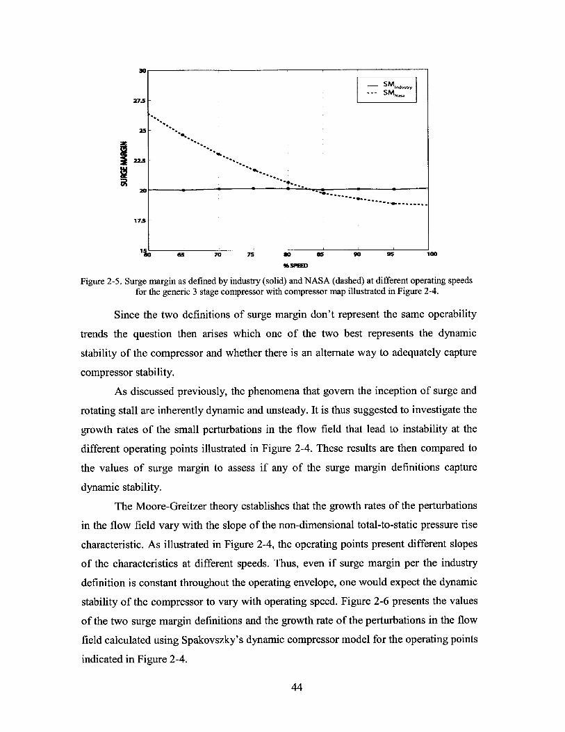
Figure 2-5. Surge margin as defined by industry (solid) and NASA (dashed) at different operating speedsfor the generic 3 stage compressor with compressor map illustrated in Figure 2-4.
Since the two definitions of surge margin don't represent the same operability
trends the question then arises which one of the two best represents the dynamic
stability of the compressor and whether there is an alternate way to adequately capture
compressor stability.
As discussed previously, the phenomena that govern the inception of surge and
rotating stall are inherently dynamic and unsteady. It is thus suggested to investigate the
growth rates of the small perturbations in the flow field that lead to instability at the
different operating points illustrated in Figure 2-4. These results are then compared to
the values of surge margin to assess if any of the surge margin definitions capture
dynamic stability.
The Moore-Greitzer theory establishes that the growth rates of the perturbations
in the flow field vary with the slope of the non-dimensional total-to-static pressure rise
characteristic. As illustrated in Figure 2-4, the operating points present different slopes
of the characteristics at different speeds. Thus, even if surge margin per the industry
definition is constant throughout the operating envelope, one would expect the dynamic
stability of the compressor to vary with operating speed. Figure 2-6 presents the values
of the two surge margin definitions and the growth rate of the perturbations in the flow
field calculated using Spakovszky's dynamic compressor model for the operating points
indicated in Figure 2-4.
44
"in
1~~~o ~~%SPEED * 9 5 i32
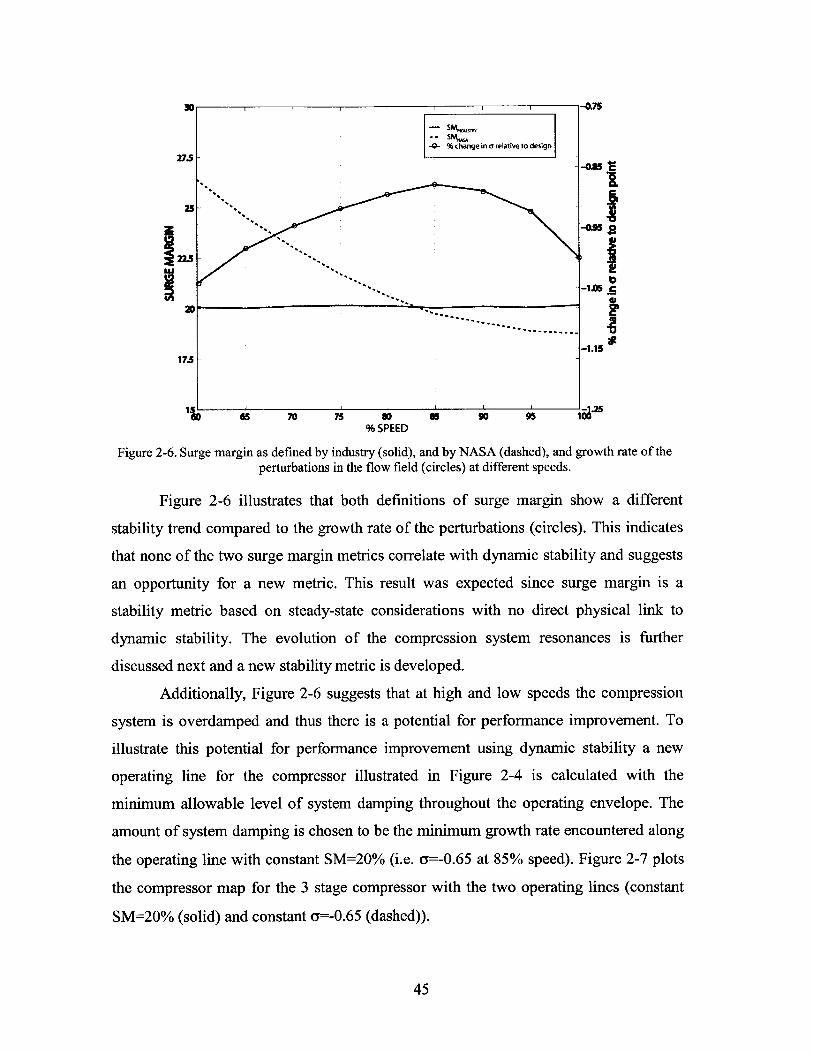
Figure 2-6. Surge margin as defined by industry (solid), and by NASA (dashed), and growth rate of theperturbations in the flow field (circles) at different speeds.
Figure 2-6 illustrates that both definitions of surge margin show a different
stability trend compared to the growth rate of the perturbations (circles). This indicates
that none of the two surge margin metrics correlate with dynamic stability and suggests
an opportunity for a new metric. This result was expected since surge margin is a
stability metric based on steady-state considerations with no direct physical link to
dynamic stability. The evolution of the compression system resonances is further
discussed next and a new stability metric is developed.
Additionally, Figure 2-6 suggests that at high and low speeds the compression
system is overdamped and thus there is a potential for performance improvement. To
illustrate this potential for performance improvement using dynamic stability a new
operating line for the compressor illustrated in Figure 2-4 is calculated with the
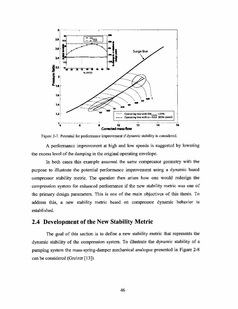
minimum allowable level of system damping throughout the operating envelope. The
amount of system damping is chosen to be the minimum growth rate encountered along
the operating line with constant SM=20% (i.e. a=-0.65 at 85% speed). Figure 2-7 plots
the compressor map for the 3 stage compressor with the two operating lines (constant
SM=20% (solid) and constant a=-0.65 (dashed)).
45
3
2.8 6ShWW
2.6-.6 ism
Surge line
2.A
2.2 is L sa7 so a so as%SPEED
2
lamSI
1.6
1.2 - Operating line with SM 20%.... Operating line with a=-0.65 (85% speed)
4 6 8 10 12 14 16Corrected mass flow
Figure 2-7. Potential for performance improvement if dynamic stability is considered.
A performance improvement at high and low speeds is suggested by lowering
the excess level of the damping in the original operating envelope.
In both cases this example assumed the same compressor geometry with the
purpose to illustrate the potential performance improvement using a dynamic based
compressor stability metric. The question then arises how one would redesign the
compression system for enhanced performance if the new stability metric was one of
the primary design parameters. This is one of the main objectives of this thesis. To
address this, a new stability metric based on compressor dynamic behavior is
established.
2.4 Development of the New Stability Metric
The goal of this section is to define a new stability metric that represents the
dynamic stability of the compression system. To illustrate the dynamic stability of a
pumping system the mass-spring-damper mechanical analogue presented in Figure 2-8
can be considered (Greizer [13]).
46
compressor
plenum
F(t)m
k throttled
compressor
y(t)
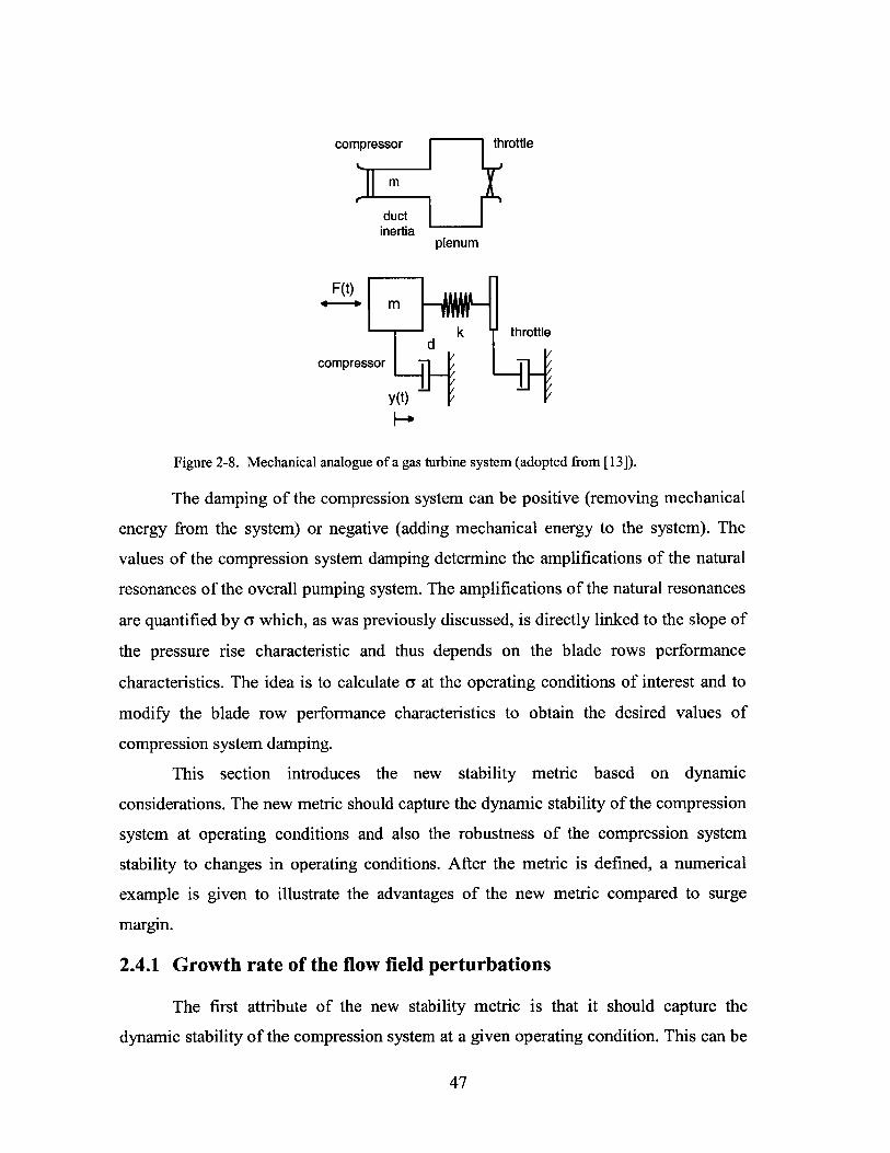
Figure 2-8. Mechanical analogue of a gas turbine system (adopted from [13]).
The damping of the compression system can be positive (removing mechanical
energy from the system) or negative (adding mechanical energy to the system). The
values of the compression system damping determine the amplifications of the natural
resonances of the overall pumping system. The amplifications of the natural resonances
are quantified by a which, as was previously discussed, is directly linked to the slope of
the pressure rise characteristic and thus depends on the blade rows performance
characteristics. The idea is to calculate a at the operating conditions of interest and to
modify the blade row performance characteristics to obtain the desired values of
compression system damping.
This section introduces the new stability metric based on dynamic
considerations. The new metric should capture the dynamic stability of the compression
system at operating conditions and also the robustness of the compression system
stability to changes in operating conditions. After the metric is defined, a numerical
example is given to illustrate the advantages of the new metric compared to surge
margin.
2.4.1 Growth rate of the flow field perturbations
The first attribute of the new stability metric is that it should capture the
dynamic stability of the compression system at a given operating condition. This can be
47
throttle
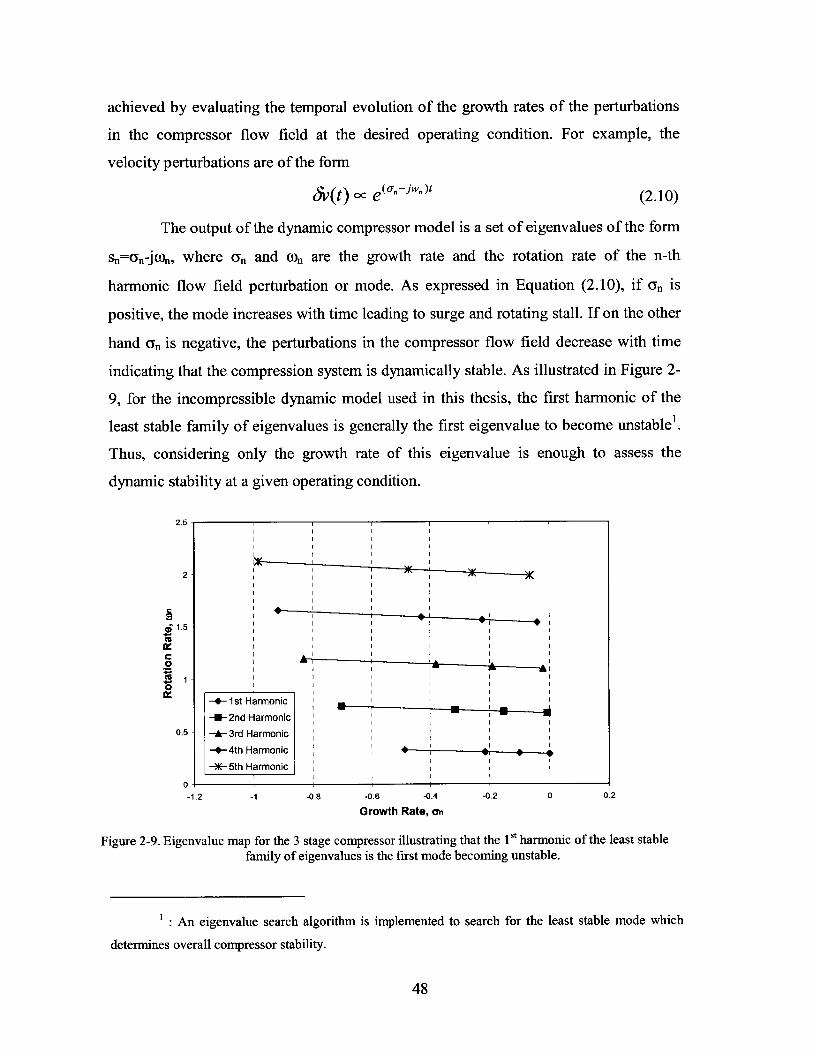
achieved by evaluating the temporal evolution of the growth rates of the perturbations
in the compressor flow field at the desired operating condition. For example, the
velocity perturbations are of the form
v(t) oc ea"w" (2.10)
The output of the dynamic compressor model is a set of eigenvalues of the form
sn=a-jon, where an and on are the growth rate and the rotation rate of the n-th
harmonic flow field perturbation or mode. As expressed in Equation (2.10), if C is
positive, the mode increases with time leading to surge and rotating stall. If on the other
hand on is negative, the perturbations in the compressor flow field decrease with time
indicating that the compression system is dynamically stable. As illustrated in Figure 2-
9, for the incompressible dynamic model used in this thesis, the first harmonic of the
least stable family of eigenvalues is generally the first eigenvalue to become unstable'.
Thus, considering only the growth rate of this eigenvalue is enough to assess the
dynamic stability at a given operating condition.
2.5 -
2
0.5
0
0.52
-1.2 -1 -0.8 -0.6 -0.4 -0.2 0 0.2
Growth Rate, an
Figure 2-9. Eigenvalue map for the 3 stage compressor illustrating that the Ist harmonic of the least stablefamily of eigenvalues is the first mode becoming unstable.
1 An eigenvalue search algorithm is implemented to search for the least stable mode which
determines overall compressor stability.
48
I I I I
I I I I
I I I I I
I I I I I
i~I( I I I
I I I
I I I I I
I I I I I
I I I
I I I I I
I I I I F
I I I I *II
I I I I I
I I I I I
I I I I
A I
I 1 IL
I I I I
I I I I I
I I I I I
I I I I
-4-1st Harmonic I I I
-4-2ndHarmonic I I II I I II I I I-~-3rd Harmonic I
-4-4th Harmonic I *, * -- 4
I I I-*--5th Harmonic I I I
I I I
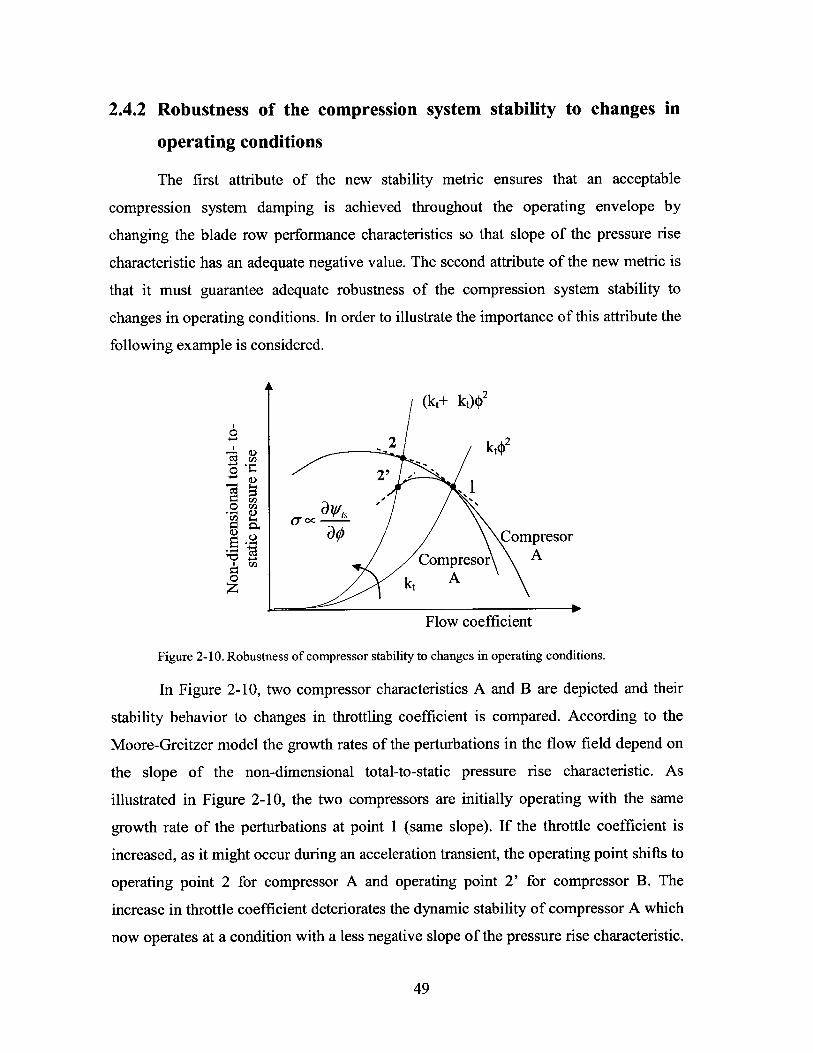
2.4.2 Robustness of the compression system stability to changes in
operating conditions
The first attribute of the new stability metric ensures that an acceptable
compression system damping is achieved throughout the operating envelope by
changing the blade row performance characteristics so that slope of the pressure rise
characteristic has an adequate negative value. The second attribute of the new metric is
that it must guarantee adequate robustness of the compression system stability to
changes in operating conditions. In order to illustrate the importance of this attribute the
following example is considered.
(kt+ kt)$2
kt2 A t
0
%YJ (X
Flow coefficient
Figure 2-10. Robustness of compressor stability to changes in operating conditions.
In Figure 2-10, two compressor characteristics A and B are depicted and their
stability behavior to changes in throttling coefficient is compared. According to the
Moore-Greitzer model the growth rates of the perturbations in the flow field depend on
the slope of the non-dimensional total-to-static pressure rise characteristic. As
illustrated in Figure 2-10, the two compressors are initially operating with the same
growth rate of the perturbations at point 1 (same slope). If the throttle coefficient is
increased, as it might occur during an acceleration transient, the operating point shifts to
operating point 2 for compressor A and operating point 2' for compressor B. The
increase in throttle coefficient deteriorates the dynamic stability of compressor A which
now operates at a condition with a less negative slope of the pressure rise characteristic.
49
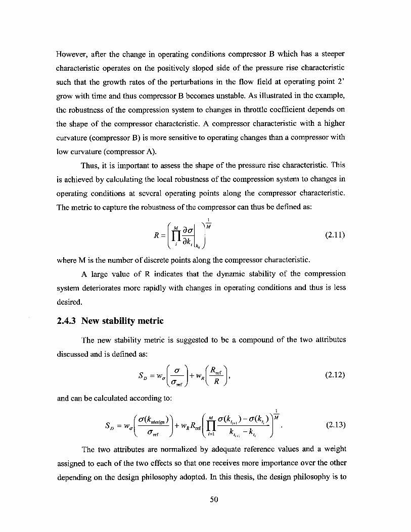
However, after the change in operating conditions compressor B which has a steeper
characteristic operates on the positively sloped side of the pressure rise characteristic
such that the growth rates of the perturbations in the flow field at operating point 2'
grow with time and thus compressor B becomes unstable. As illustrated in the example,
the robustness of the compression system to changes in throttle coefficient depends on
the shape of the compressor characteristic. A compressor characteristic with a higher
curvature (compressor B) is more sensitive to operating changes than a compressor with
low curvature (compressor A).
Thus, it is important to assess the shape of the pressure rise characteristic. This
is achieved by calculating the local robustness of the compression system to changes in
operating conditions at several operating points along the compressor characteristic.
The metric to capture the robustness of the compressor can thus be defined as:
R = o (2.11)
where M is the number of discrete points along the compressor characteristic.
A large value of R indicates that the dynamic stability of the compression
system deteriorates more rapidly with changes in operating conditions and thus is less
desired.
2.4.3 New stability metric
The new stability metric is suggested to be a compound of the two attributes
discussed and is defined as:
SD = w. + WR ref (2.12)Orref R
and can be calculated according to:
(= (kt'esjgn rr. a(k,)-a(k,SD ' tdesig WRRLI ( ' ' I. (2.13)
ref Ji=1 t
The two attributes are normalized by adequate reference values and a weight
assigned to each of the two effects so that one receives more importance over the other
depending on the design philosophy adopted. In this thesis, the design philosophy is to
50
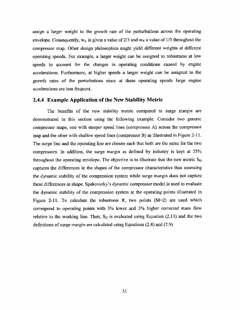
assign a larger weight to the growth rate of the perturbations across the operating
envelope. Consequently, w, is given a value of 2/3 and WR a value of 1/3 throughout the
compressor map. Other design philosophies might yield different weights at different
operating speeds. For example, a larger weight can be assigned to robustness at low
speeds to account for the changes in operating conditions caused by engine
accelerations. Furthermore, at higher speeds a larger weight can be assigned to the
growth rates of the perturbations since at these operating speeds large engine
accelerations are less frequent.
2.4.4 Example Application of the New Stability Metric
The benefits of the new stability metric compared to surge margin are
demonstrated in this section using the following example. Consider two generic
compressor maps, one with steeper speed lines (compressor A) across the compressor
map and the other with shallow speed lines (compressor B) as illustrated in Figure 2-11.
The surge line and the operating line are chosen such that both are the same for the two
compressors. In addition, the surge margin as defined by industry is kept at 25%
throughout the operating envelope. The objective is to illustrate that the new metric SD
captures the differences in the shapes of the compressor characteristics thus assessing
the dynamic stability of the compression system while surge margin does not capture
these differences in shape. Spakovszky's dynamic compressor model is used to evaluate
the dynamic stability of the compression system at the operating points illustrated in
Figure 2-11. To calculate the robustness R, two points (M=2) are used which
correspond to operating points with 3% lower and 3% higher corrected mass flow
relative to the working line. Then, SD is evaluated using Equation (2.13) and the two
definitions of surge margin are calculated using Equations (2.8) and (2.9)
51
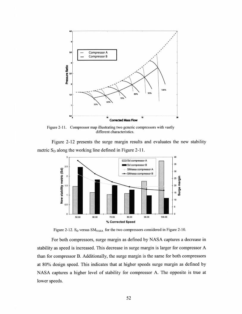
45
4
3
15
5
G51
5
- Compressor A-- Compressor B
100%
1O isCorrected Mass Flow
Figure 2-11. Compressor map illustrating two generic compressors with vastlydifferent characteristics.
a
Figure 2-12 presents the surge margin results and evaluates
metric SD along the working line defined in Figure 2-11.3 ,
2.5
.
1
3
0.5
0
40
35
30
25
20
15
10
5
0
IM
0M
50.00 60.00 70.00 80.00 90.00 100.00
% Corrected Speed
Figure 2-12. SD versus SMNASA for the two compressors considered in Figure 2-10.
For both compressors, surge margin as defined by NASA captures a decrease in
stability as speed is increased. This decrease in surge margin is larger for compressor A
than for compressor B. Additionally, the surge margin is the same for both compressors
at 80% design speed. This indicates that at higher speeds surge margin as defined by
NASA captures a higher level of stability for compressor A. The opposite is true at
lower speeds.
52
the new stability
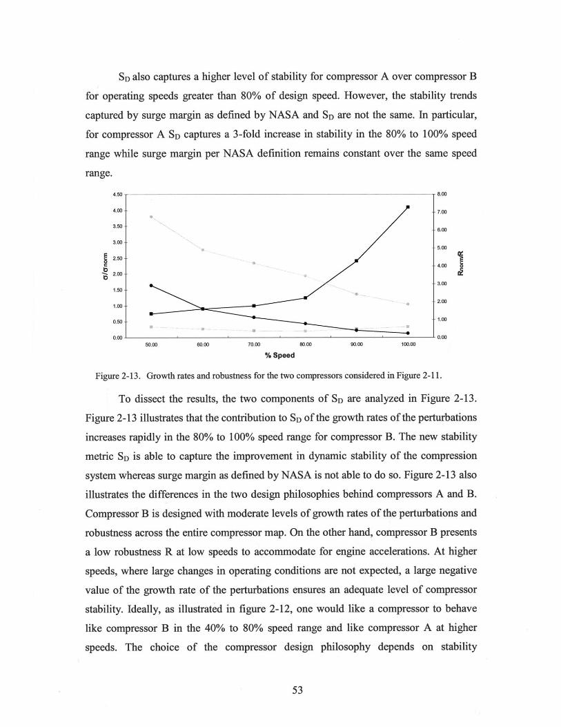
SD also captures a higher level of stability for compressor A over compressor B
for operating speeds greater than 80% of design speed. However, the stability trends
captured by surge margin as defined by NASA and SD are not the same. In particular,
for compressor A SD captures a 3-fold increase in stability in the 80% to 100% speed
range while surge margin per NASA definition remains constant over the same speed
range.
4.50 8.00
4.00- 7.00
3.506.3 06.00
3.0045200
2.50-3
.200-.00-3.00
1.50-
1.000
0.50-- -- 1.00
0.00 0.0050.00 60.00 70.00 80.00 90.00 100.00
%Speed
Figure 2-13. Growth rates and robustness for the two compressors considered in Figure 2-11.
To dissect the results, the two components of SD are analyzed in Figure 2-13.
Figure 2-13 illustrates that the contribution to SD of the growth rates of the perturbations
increases rapidly in the 80% to 100% speed range for compressor B. The new stability
metric SD is able to capture the improvement in dynamic stability of the compression
system whereas surge margin as defined by NASA is not able to do so. Figure 2-13 also
illustrates the differences in the two design philosophies behind compressors A and B.
Compressor B is designed with moderate levels of growth rates of the perturbations and
robustness across the entire compressor map. On the other hand, compressor B presents
a low robustness R at low speeds to accommodate for engine accelerations. At higher
speeds, where large changes in operating conditions are not expected, a large negative
value of the growth rate of the perturbations ensures an adequate level of compressor
stability. Ideally, as illustrated in figure 2-12, one would like a compressor to behave
like compressor B in the 40% to 80% speed range and like compressor A at higher
speeds. The choice of the compressor design philosophy depends on stability
53
considerations at low speeds and at high speeds and the compromises to be made
between design and off-design conditions.
This example shows that surge margin as defined by industry does not correlate
in any way with dynamic stability and that surge margin as defined by NASA follows
qualitatively the stability trends shown by SD. However, SD captures the dynamic
stability of the compression system and the sensitivity of stability to working line
changes (i.e. shape of the characteristics) which neither of the two surge margins
account for. Taking advantage of these features, the new stability metric, if used in the
design phase as a prime design variable, suggests compressor designs with enhanced
performance and dynamic stability. This is the focus of the remainder of the thesis.
2.5 Summary
This chapter demonstrates that neither of the two surge margin definitions used
in the field to evaluate compressor stability correlate with dynamic stability. In addition,
the potential for performance improvement is illustrated by removing the excessive
damping levels in the compression system due to the current surge margin constraints.
To take advantage of the shortcomings of the conventional stability metrics a new
stability metric based on dynamic considerations (SD) is defined. SD is a compound of
two attributes: the growth rates of the perturbations in the flow field (i.e. slope of the
pressure rise characteristic) and the sensitivity of compressor stability to working line
changes (i.e. shape of the pressure rise characteristic).
The advantages of SD compared to surge margin are demonstrated using an
example with two vastly different compressor characteristics. The results show that
while surge margin per industry definition does not correlate with dynamic stability,
surge margin per NASA definition can assess qualitatively some of the trends. However
only the new stability metric SD is able to quantitatively capture the dynamic stability of
the compression system. This suggests to use SD as the new metric throughout the
remainder of this thesis in conjunction with a compressor design methodology to
enhance compressor performance and stability.
54
Chapter 3
Fast Blade Performance PredictionMethod
This chapter briefly motivates for the new fast blade performance prediction
method and describes previous efforts using similar methodologies. Then, the three
stepping-stones required to create the blade performance prediction method are
discussed. These are the definition and the assessment of a new blade parameterization
scheme. The generation of a blade performance database to define a new blade family,
and the implementation of an N-dimensional linear interpolation to estimate the
performance of a given blade row geometry. In addition, the accuracy and speed of the
blade performance prediction method are compared to direct CFD simulations to assess
the new approach.
3.1 Motivation
As discussed in Chapter 1, the preliminary compressor design phase entails the
evaluation of the performance and operability of various compressor architectures. As
discussed in Chapter 2, to calculate the dynamic stability of a compression system the
slope of the blade row loss characteristics with respect to axial and tangential velocities
is required (Equations (2.3), (2.4) and (2.5)). Consequently, to evaluate the compressor
performance and stability the compressor blade row losses need to be calculated. These
losses can be divided into profile losses and 3D loss effects such as for example end
wall loss. One of the goals of this thesis is to develop a new compressor design
methodology and to conduct proof-of-concept studies. To do so a 2D approach has been
adopted. This assumption is appropriate since compressor geometries with high hub-to-
tip radius ratios are considered where 3D loss effects are less important. These blade
55
row profile losses can be obtained either using experimental data or computational fluid
dynamics (CFD). Since CFD allows a flexible design of cascade configurations and a
fast evaluation of their performance, numerical simulations are used in this thesis to
evaluate the profile losses of the different compressor configurations. Particularly, the
blade-to-blade flow solver MISES [29] is used to do so.
The compressor optimization design based on the framework introduced in this
thesis (Figure 1-8) requires the evaluation of the performance and stability of over one
thousand compressor designs. If the profile losses of the compressor blade rows are
evaluated using CFD in each iteration, the compressor optimization would require
approximately 17 days. To reduce such a long turn around time a faster blade
performance prediction method needs to be developed.
3.2 Previous Work
CFD based design methods use interpolation methods on previously gathered
CFD information to estimate the performance of a given blade row. Perrot [21]
proposes a CFD based method to predict the losses of an airfoil for different values of
stagger. The method uses a least square fit of a surface to a set of CFD data points. The
parameters considered are stagger angle and incidence angle and a surface fit according
to:
w(iy) =co +c1 i+c 2y+c3 iy+ci 2 +c5 i3 y+c6 i4 (3.1)
is used which allows twists and narrowings of the surface as the incidence and stagger
angle are varied.
The results show that the discrepancy between the surface fit and the CFD data
is too large for this methodology to be used in a compressor design optimization
framework. Moreover, the method is limited to low Mach numbers (of order 0.1) and to
variations in one geometric parameter (stagger angle varying in a +30 range of the
baseline value). Adding more geometric parameters and increasing the Mach numbers
to open the design space and improve the performance of the optimizer requires a multi-
dimensional surface fit which will further deteriorate the discrepancies between the
CFD data and the surface fit.
56
Perrot's effort indicates that creating an accurate and fast method linking
geometry, incidence and Mach number to blade performance is quite a challenge. The
new CFD based method proposed in this thesis needs to be more accurate and needs to
include more parameters than Perrot's method to enable performance and operability
enhancement in the compressor design.
The approach is as follows. A blade parameterization is created and bounds on
the geometric parameters are set to generate a new family of blades. Then the new
family of blades is simulated using the blade-to-blade flow solver MISES and the blade
performance information is stored using MATLAB to create a blade performance
database. Finally, an N-dimensional linear interpolation between the blade performance
files obtained from CFD is implemented which ensure accurate and fast blade
performance estimates.
3.3 Blade Parameterization
The fast blade performance prediction method requires a family of blades to be
generated. This blade family needs to represent various blade row designs such that the
compressor design optimization framework can evaluate different compressor
architectures. In addition the set of blades needs to include the minimum possible
number of blade row geometries possible to reduce the CFD computational efforts.
Consequently, a simple and versatile blade parameterization is required.
Sieverding et al. [23] propose a flexible blade parameterization to optimize an
airfoil profile for minimum loss and maximum width of the loss bucket. The blade
geometry is determined using 20 parameters. Two major inconveniences arise if this
parameterization is considered to generate the required set of cascade geometries. The
first problem is that the acceptable bounds on each of the 20 parameters are unknown
with no a priori experience available on these parameters. Furthermore, the major
disadvantage of this blade parameterization is that at least two sets (a lower and an
upper bound) of each of the parameters need to be calculated to create a blade
performance database. This implies that 220 blades need to be simulated. Thus a simpler
blade parameterization is needed to avoid the costly simulation of such a large amount
of blades.
57
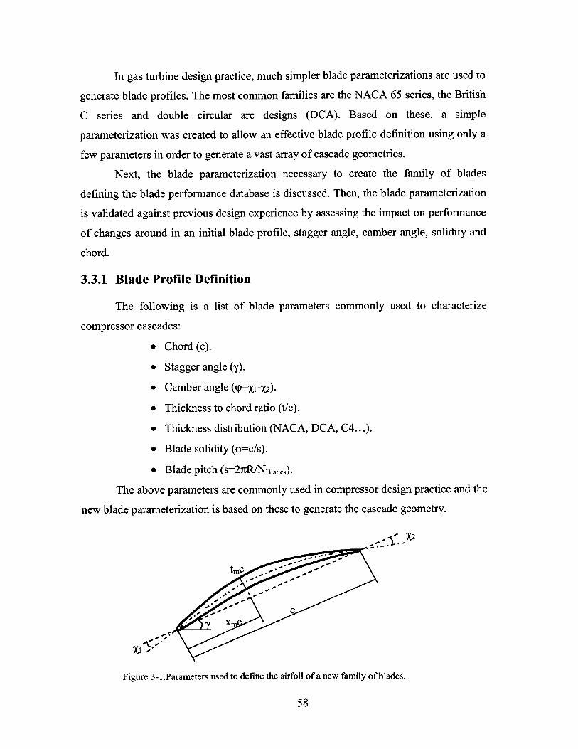
In gas turbine design practice, much simpler blade parameterizations are used to
generate blade profiles. The most common families are the NACA 65 series, the British
C series and double circular arc designs (DCA). Based on these, a simple
parameterization was created to allow an effective blade profile definition using only a
few parameters in order to generate a vast array of cascade geometries.
Next, the blade parameterization necessary to create the family of blades
defining the blade performance database is discussed. Then, the blade parameterization
is validated against previous design experience by assessing the impact on performance
of changes around in an initial blade profile, stagger angle, camber angle, solidity and
chord.
3.3.1 Blade Profile Definition
The following is a list of blade parameters commonly used to characterize
compressor cascades:
" Chord (c).
" Stagger angle (y).
" Camber angle (p=XI-X2).
" Thickness to chord ratio (t/c).
" Thickness distribution (NACA, DCA, C4...).
" Blade solidity (a=c/s).
" Blade pitch (s=2nR/NBades)-
The above parameters are commonly used in compressor design practice and the
new blade parameterization is based on these to generate the cascade geometry.
- X2
r - .
Figure 3 -1. Parameters used to define the airfoil of a new family of blades.
58
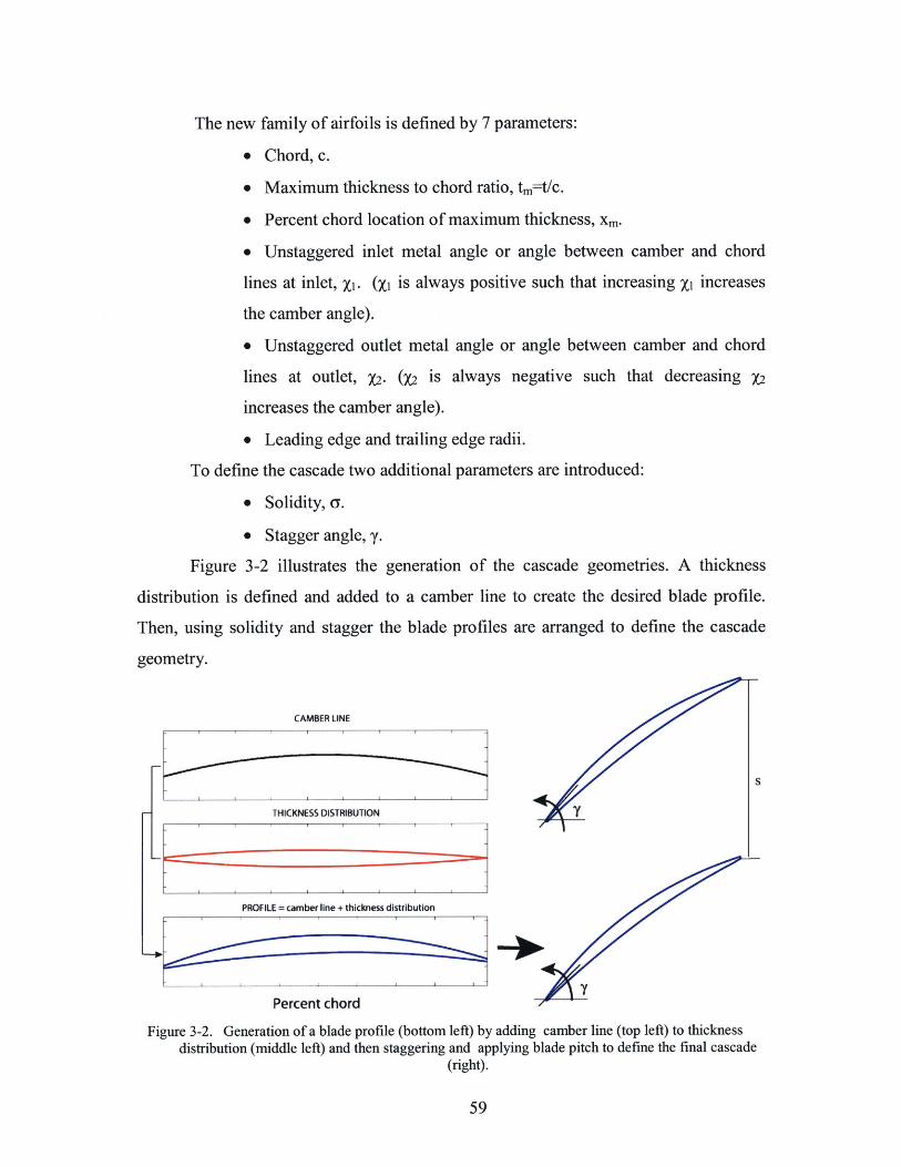
The new family of airfoils is defined by 7 parameters:
" Chord, c.
* Maximum thickness to chord ratio, tm=t/c.
" Percent chord location of maximum thickness, Xm.
* Unstaggered inlet metal angle or angle between camber and chord
lines at inlet, X1. (Xi is always positive such that increasing X1 increases
the camber angle).
* Unstaggered outlet metal angle or angle between camber and chord
lines at outlet, X2. (y2 is always negative such that decreasing X2
increases the camber angle).
* Leading edge and trailing edge radii.
To define the cascade two additional parameters are introduced:
* Solidity, a.
" Stagger angle, y.
Figure 3-2 illustrates the generation of the cascade geometries. A thickness
distribution is defined and added to a camber line to create the desired blade profile.
Then, using solidity and stagger the blade profiles are arranged to define the cascade
geometry.
CAMBER LINE
S
THICKNESS DISTRIBUTION 7
PROFILE = camber line + thickness distribution
Percent chord
Figure 3-2. Generation of a blade profile (bottom left) by adding camber line (top left) to thicknessdistribution (middle left) and then staggering and applying blade pitch to define the final cascade
(right).
59
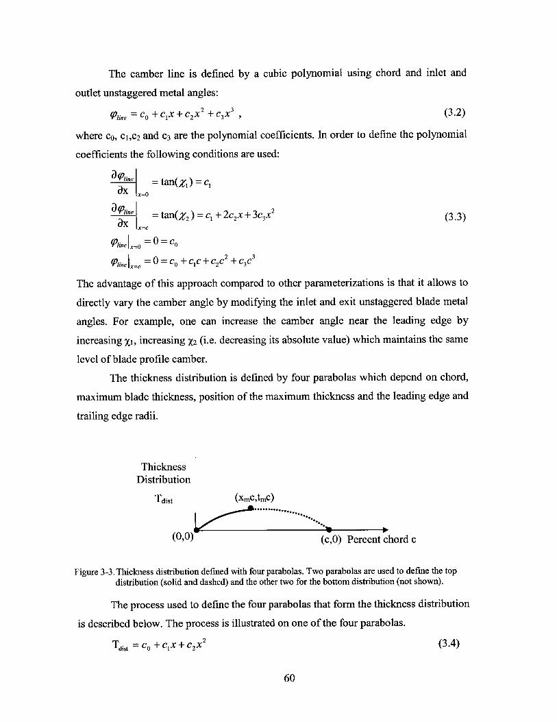
The camber line is defined by a cubic polynomial using chord and inlet and
outlet unstaggered metal angles:
Oine = Co +CiX+C 2 X2 +C 3 X , (3.2)
where co, c1,c2 and c3 are the polynomial coefficients. In order to define the polynomial
coefficients the following conditions are used:
(Piune = tan(zi)= C1ax Xx=O
a (Oune = tan(X2 ) c + 2c 2x+3c3x 2 (3.3)
-Ix X=
(O|ine-O 0 = =cO
ine I | =0=cO+cIc+c 2c 2 +c 3c3
The advantage of this approach compared to other parameterizations is that it allows to
directly vary the camber angle by modifying the inlet and exit unstaggered blade metal
angles. For example, one can increase the camber angle near the leading edge by
increasing X1, increasing X2 (i.e. decreasing its absolute value) which maintains the same
level of blade profile camber.
The thickness distribution is defined by four parabolas which depend on chord,
maximum blade thickness, position of the maximum thickness and the leading edge and
trailing edge radii.
ThicknessDistribution
Tdist (xmc,tmc)....... ...............
(0,0) (c,0) Percent chord c
Figure 3-3. Thickness distribution defined with four parabolas. Two parabolas are used to define the topdistribution (solid and dashed) and the other two for the bottom distribution (not shown).
The process used to define the four parabolas that form the thickness distribution
is described below. The process is illustrated on one of the four parabolas.
Tdist = co + c1x + 2X2 (3.4)
60
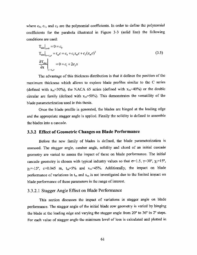
where co, ci, and c2 are the polynomial coefficients. In order to define the polynomial
coefficients for the parabola illustrated in Figure 3-3 (solid line) the following
conditions are used:
T = 0 = co
TdistI x=xmC = tmc = co + cIx,,c + c2 (XMC) 2 (3.5)
aTdist 0 = C +2C2Xax
X=XmC
The advantage of this thickness distribution is that it defines the position of the
maximum thickness which allows to explore blade profiles similar to the C series
(defined with xm=30%), the NACA 65 series (defined with xm=40%) or the double
circular arc family (defined with xm=50%). This demonstrates the versatility of the
blade parameterization used in this thesis.
Once the blade profile is generated, the blades are hinged at the leading edge
and the appropriate stagger angle is applied. Finally the solidity is defined to assemble
the blades into a cascade.
3.3.2 Effect of Geometric Changes on Blade Performance
Before the new family of blades is defined, the blade parameterization is
assessed. The stagger angle, camber angle, solidity and chord of an initial cascade
geometry are varied to assess the impact of these on blade performance. The initial
cascade geometry is chosen with typical industry values so that a=1.5, y=30*, Xi=15*,
X1=-15*, c=0.045 m, tm=5% and xm=45%. Additionally, the impact on blade
performance of variations in tm and xm is not investigated due to the limited impact on
blade performance of these parameters in the range of interest.
3.3.2.1 Stagger Angle Effect on Blade Performance
This section discusses the impact of variations in stagger angle on blade
performance. The stagger angle of the initial blade row geometry is varied by hinging
the blade at the leading edge and varying the stagger angle from 20* to 360 in 20 steps.
For each value of stagger angle the minimum level of loss is calculated and plotted in
61
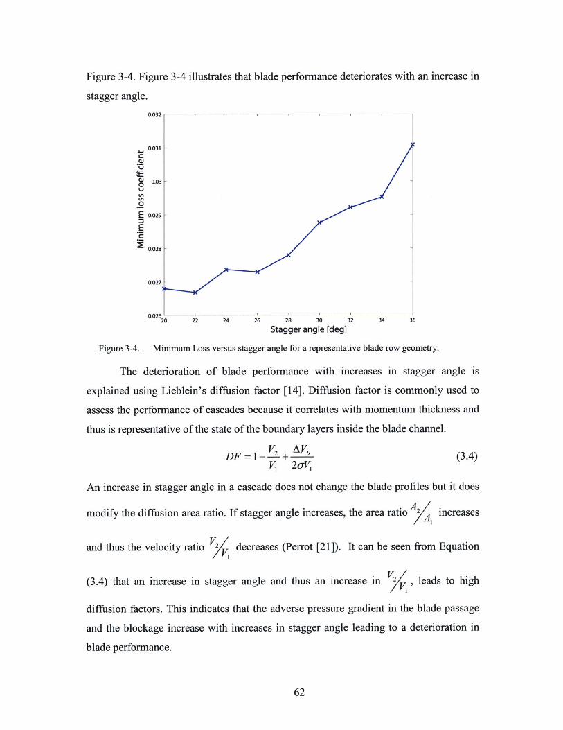
Figure 3-4. Figure
stagger angle.
3-4 illustrates that blade performance deteriorates with an increase in
0.032 - - T
0.031 -
0.030
0
E 0.029
0.028
0.027-
20 22 24 26 28 30 32
Stagger angle [deg]
Figure 3-4. Minimum Loss versus stagger angle for a representative
The deterioration of blade performance with increases in stagger angle is
explained using Lieblein's diffusion factor [14]. Diffusion factor is commonly used to
assess the performance of cascades because it correlates with momentum thickness and
thus is representative of the state of the boundary layers inside the blade channel.
DF =1 -2+ V2 (3.4)V, 2-V,
An increase in stagger angle in a cascade does not change the blade profiles but it does
modify the diffusion area ratio. If stagger angle increases, the area ratio A increasesA1
and thus the velocity ratio V decreases (Perrot [21]). It can be seen from Equation
(3.4) that an increase in stagger angle and thus an increase in V , leads to high
diffusion factors. This indicates that the adverse pressure gradient in the blade passage
and the blockage increase with increases in stagger angle leading to a deterioration in
blade performance.
62
34 36
blade row geometry.
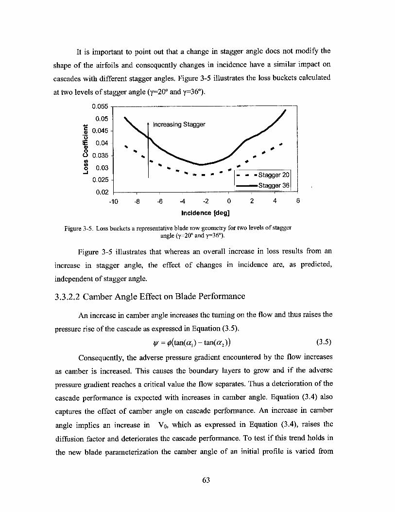
It is important to point out that a change in stagger angle does not modify the
shape of the airfoils and consequently changes in incidence have a similar impact on
cascades with different stagger angles. Figure 3-5 illustrates the loss buckets calculated
at two levels of stagger angle (y=2 0" and y=36*).
0.0551
0.05-Increasing Stagger
* 0.045-
S0.04 -
0 0.035 -
0 0.03- - ,
0.025-- - -Stagger 20
- Stagger 360.02 1 1
-10 -8 -6 -4 -2 0 2 4 6
Incidence [deg]
Figure 3-5. Loss buckets a representative blade row geometry for two levels of stagger
angle (y=2 0 " and y=36*).
Figure 3-5 illustrates that whereas an overall increase in loss results from an
increase in stagger angle, the effect of changes in incidence are, as predicted,
independent of stagger angle.
3.3.2.2 Camber Angle Effect on Blade Performance
An increase in camber angle increases the turning on the flow and thus raises the
pressure rise of the cascade as expressed in Equation (3.5).
Vr = $(tan(al) - tan(a 2 )) (3.5)
Consequently, the adverse pressure gradient encountered by the flow increases
as camber is increased. This causes the boundary layers to grow and if the adverse
pressure gradient reaches a critical value the flow separates. Thus a deterioration of the
cascade performance is expected with increases in camber angle. Equation (3.4) also
captures the effect of camber angle on cascade performance. An increase in camber
angle implies an increase in VO, which as expressed in Equation (3.4), raises the
diffusion factor and deteriorates the cascade performance. To test if this trend holds in
the new blade parameterization the camber angle of an initial profile is varied from
63
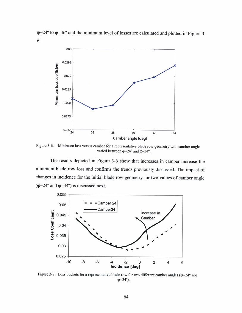
<p=24* to (p=36* and the minimum level of losses are calculated and plotted in Figure 3-
6.
0.03
4-0C:
0
0
EE
0.0295
0.029
0.0285
0.028
0.0275
0.027 '24 26 28 30 32 34
Camber angle [deg]
Figure 3-6. Minimum loss versus camber for a representative blade row geometry with camber anglevaried between <p=24 0 and (p=34*.
The results depicted in Figure 3-6 show that increases in camber increase the
minimum blade row loss and confirms the trends previously discussed. The impact of
changes in incidence for the initial blade row geometry for two values of camber angle
(p=24* and (p=34*) is discussed next.
0.0551
*0
a,00
-j
0.05-
0.045 -
0.04 -
0.035 -
0.03 -
0.025 l
-10
Figure 3-7. Loss buckets
I I III1
-8 -6 -4 -2 0 2 4 6Incidence [deg]
for a representative blade row for two different camber angles (<p=24* and(p=34*).
64
- - - Camber 24
-- Camber34Increase in
9*
a
% W
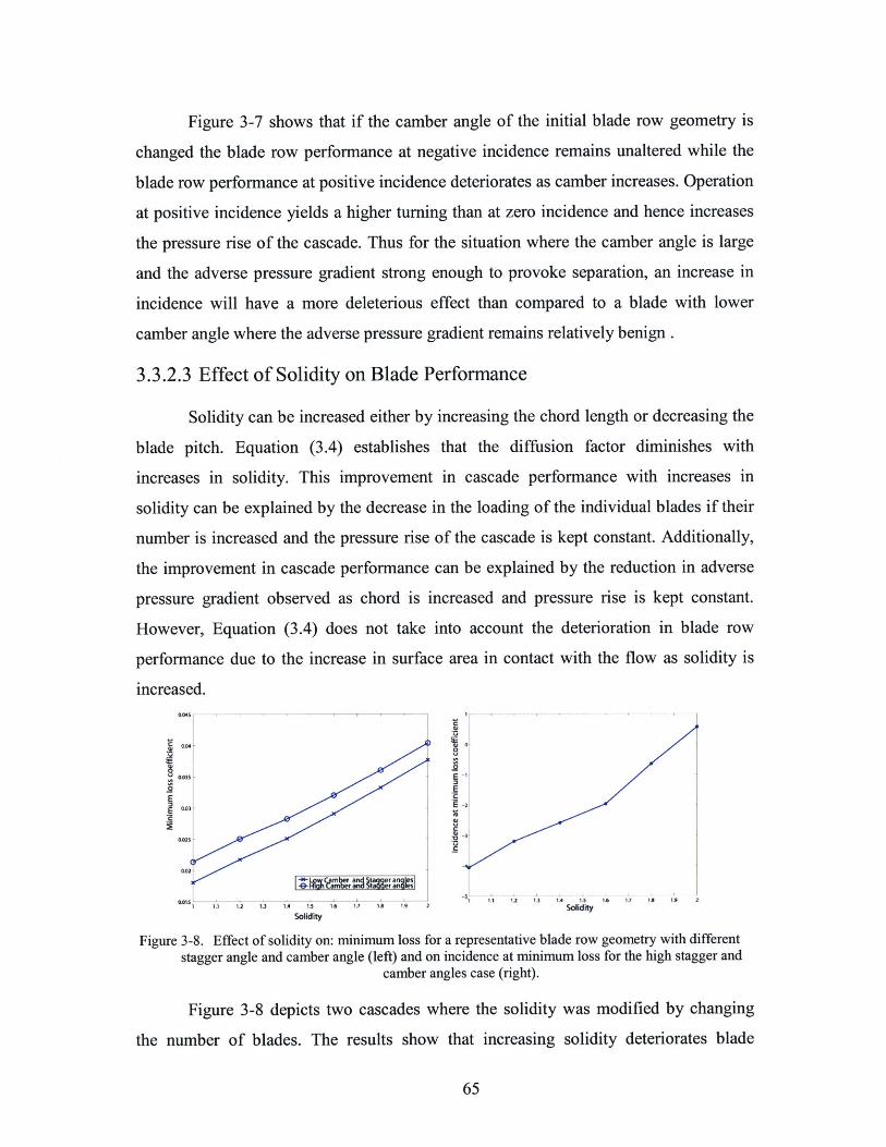
Figure 3-7 shows that if the camber angle of the initial blade row geometry is
changed the blade row performance at negative incidence remains unaltered while the
blade row performance at positive incidence deteriorates as camber increases. Operation
at positive incidence yields a higher turning than at zero incidence and hence increases
the pressure rise of the cascade. Thus for the situation where the camber angle is large
and the adverse pressure gradient strong enough to provoke separation, an increase in
incidence will have a more deleterious effect than compared to a blade with lower
camber angle where the adverse pressure gradient remains relatively benign .
3.3.2.3 Effect of Solidity on Blade Performance
Solidity can be increased either by increasing the chord length or decreasing the
blade pitch. Equation (3.4) establishes that the diffusion factor diminishes with
increases in solidity. This improvement in cascade performance with increases in
solidity can be explained by the decrease in the loading of the individual blades if their
number is increased and the pressure rise of the cascade is kept constant. Additionally,
the improvement in cascade performance can be explained by the reduction in adverse
pressure gradient observed as chord is increased and pressure rise is kept constant.
However, Equation (3.4) does not take into account the deterioration in blade row
performance due to the increase in surface area in contact with the flow as solidity is
increased.
0.04-
0 EESE 0.03 E-
cabera a s e0.1 - - -" 1.2 1.3 IA4 i 1.3 1.7 1 A 1.9 2
1 11 13 1.4 5 1.6 1.7 1 1.9 2SofiditySolidity
Figure 3-8. Effect of solidity on: minimum loss for a representative blade row geometry with differentstagger angle and camber angle (left) and on incidence at minimum loss for the high stagger and
camber angles case (right).
Figure 3-8 depicts two cascades where the solidity was modified by changing
the number of blades. The results show that increasing solidity deteriorates blade
65
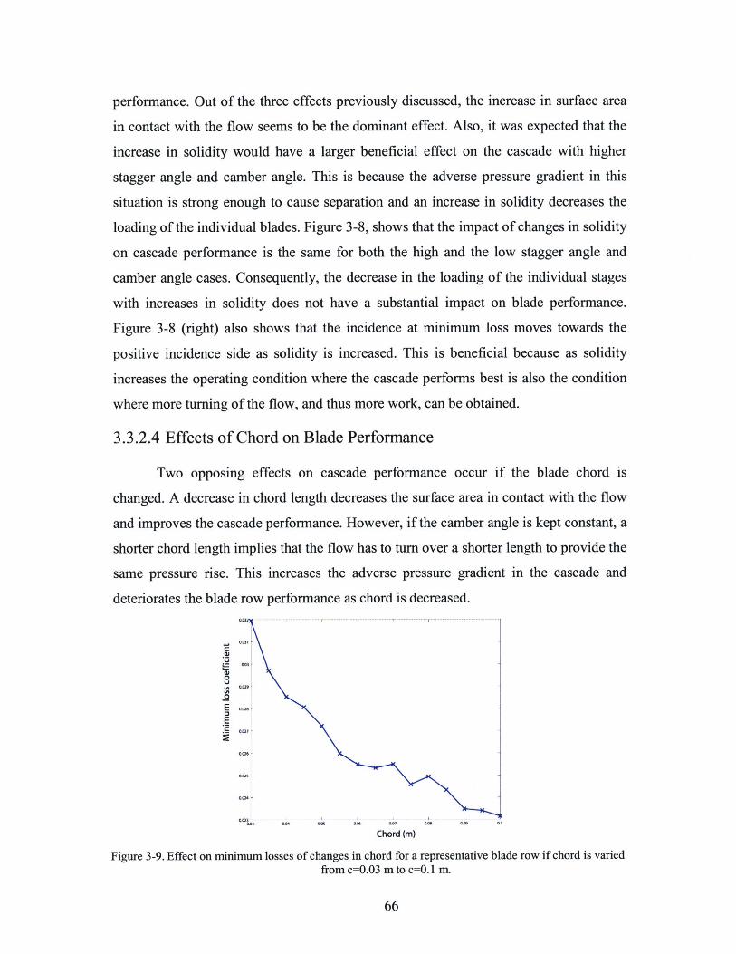
performance. Out of the three effects previously discussed, the increase in surface area
in contact with the flow seems to be the dominant effect. Also, it was expected that the
increase in solidity would have a larger beneficial effect on the cascade with higher
stagger angle and camber angle. This is because the adverse pressure gradient in this
situation is strong enough to cause separation and an increase in solidity decreases the
loading of the individual blades. Figure 3-8, shows that the impact of changes in solidity
on cascade performance is the same for both the high and the low stagger angle and
camber angle cases. Consequently, the decrease in the loading of the individual stages
with increases in solidity does not have a substantial impact on blade performance.
Figure 3-8 (right) also shows that the incidence at minimum loss moves towards the
positive incidence side as solidity is increased. This is beneficial because as solidity
increases the operating condition where the cascade performs best is also the condition
where more turning of the flow, and thus more work, can be obtained.
3.3.2.4 Effects of Chord on Blade Performance
Two opposing effects on cascade performance occur if the blade chord is
changed. A decrease in chord length decreases the surface area in contact with the flow
and improves the cascade performance. However, if the camber angle is kept constant, a
shorter chord length implies that the flow has to turn over a shorter length to provide the
same pressure rise. This increases the adverse pressure gradient in the cascade and
deteriorates the blade row performance as chord is decreased.
0.024 --
0M
0
E
M 04 0 06 00 00 0.03 01
Chord (m)
Figure 3-9. Effect on minimum losses of changes in chord for a representative blade row if chord is variedfrom c=0.03 m to c=O. 1 m.
66

The blade chord of the initial geometry is varied from c=0.03 to c=O. 1 and for
each of the cases studied the minimum level of loss is calculated. Figure 3-9 shows that
an increase in chord is beneficial. Consequently, in the example considered, this
indicates that reducing the adverse pressure gradient has a larger impact on cascade
performance than increasing the surface area in contact with the flow.
3.4 Blade Performance Prediction Method
The blade performance prediction method uses an N-dimensional linear
interpolation between the blade performance files obtained from CFD to estimate the
performance of a given geometry.
Having established the blade parameterization, the family of blades necessary to
generate the blade performance database needs to be defined. This requires a choice of
the range in geometric parameters that define the blade family. Then, the blade row
geometries are simulated using an automated blade-to-blade CFD utility (MISES).
Finally the N-dimensional linear interpolation method is implemented to predict the
performance of the desired cascade geometry. Last, the accuracy of the new
performance prediction method is assessed.
3.4.1 Blade Family
The ranges of the geometric parameters used to define the family of blades used
in this thesis are summarized in Table 3-1. The range in geometric parameters is based
on compressor design practice and on the limits of the convergence of the CFD method
used in this thesis.
XI X2 Chord Stagger[deg [de] Solidity angle xm (%)
[deg] [deg] (in) [deg]Minimum 10 -15 0.03 1.5 20 30
Value____
Maximum 20 -10 0.05 2 35 50Value ____
Number ofpoints 4 1 3 1 6 1
betweenbounds
Table 3-1. Recommended ranges of geometric parameters to define the blade family.
67
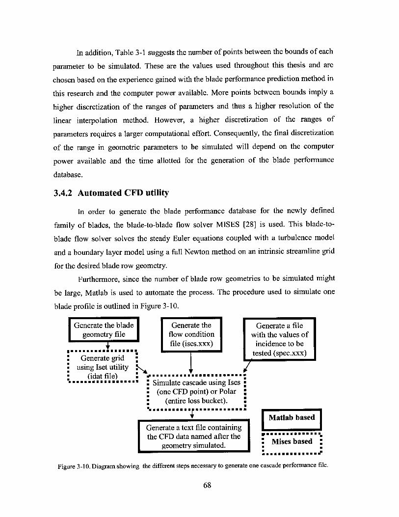
In addition, Table 3-1 suggests the number of points between the bounds of each
parameter to be simulated. These are the values used throughout this thesis and are
chosen based on the experience gained with the blade performance prediction method in
this research and the computer power available. More points between bounds imply a
higher discretization of the ranges of parameters and thus a higher resolution of the
linear interpolation method. However, a higher discretization of the ranges of
parameters requires a larger computational effort. Consequently, the final discretization
of the range in geometric parameters to be simulated will depend on the computer
power available and the time allotted for the generation of the blade performance
database.
3.4.2 Automated CFD utility
In order to generate the blade performance database for the newly defined
family of blades, the blade-to-blade flow solver MISES [28] is used. This blade-to-
blade flow solver solves the steady Euler equations coupled with a turbulence model
and a boundary layer model using a full Newton method on an intrinsic streamline grid
for the desired blade row geometry.
Furthermore, since the number of blade row geometries to be simulated might
be large, Matlab is used to automate the process. The procedure used to simulate one
blade profile is outlined in Figure 3-10.
Generate the blade Generate the Generate a filegeometry file flow condition with the values of
file (ises.xxx) incidence to be""""""""""""""""". tested (spec.xxx). Generate grid ;
"using Iset utility(idat file) " -""U""""""E":EUEUEEo
" Simulate cascade using Ises ;(one CFD point) or Polar :
(entire loss bucket). "
Matlab basedGenerate a text file containingthe CFD data named after the "
geometry simulated. Mises based "
Figure 3-10. Diagram showing the different steps necessary to generate one cascade performance file.
68
Figure 3-10 illustrates the different steps required to obtain a blade performance
file. Initially, the coordinates of the blade, the flow conditions (Mach number and
Reynolds number) and the incidence angles are written into three files using Matlab.
Then, the grid is generated using the blade geometry file. The result is a file (idat)
containing the grid information. Then, Ises or Polar calculate the performance of the
cascade using the grid file (idat), the flow condition file (ises) and the file containing the
incidence angles to be simulated (spec). Once the performance of the cascade is
calculated, the output file from MISES is opened using Matlab and the data is rewritten
into a text file containing incidence, Mach number and performance information. This
file is named after the geometry that was simulated. Then, the process is repeated for all
cascade geometries to generate the blade performance database to be used by the
interpolation method in the compressor design optimization framework.
3.4.3 Interpolation Method
In order to predict the performance of a given blade row geometry an N-
dimensional linear interpolation between the blade performance files is implemented.
The method is effective since it provides the necessary blade performance estimates in
less than 0.1 seconds. This is 1/100 of the average time required by MISES to calculate
one operating point. Furthermore, the blade performance prediction method must
provide accurate results since the fidelity of the blade performance prediction method is
crucial to the overall success of the optimization framework. This is discussed next.
3.4.4 Resolution of the blade performance prediction method
The results of the blade performance prediction method need to be as accurate as
possible. This is important because during the optimization process many compressor
designs are evaluated and a small inaccuracy in the performance calculation at the
beginning of the compressor optimization can lead to an inadequate compressor design
at the end of the process.
To assess the accuracy and fidelity of the blade performance prediction method,
the blade row losses of the baseline 3 stage compressor which are used throughout this
thesis (refer to Chapter 4 for more details on the compressor geometry) are directly
calculated using MISES and are compared to the predictions using the blade
69
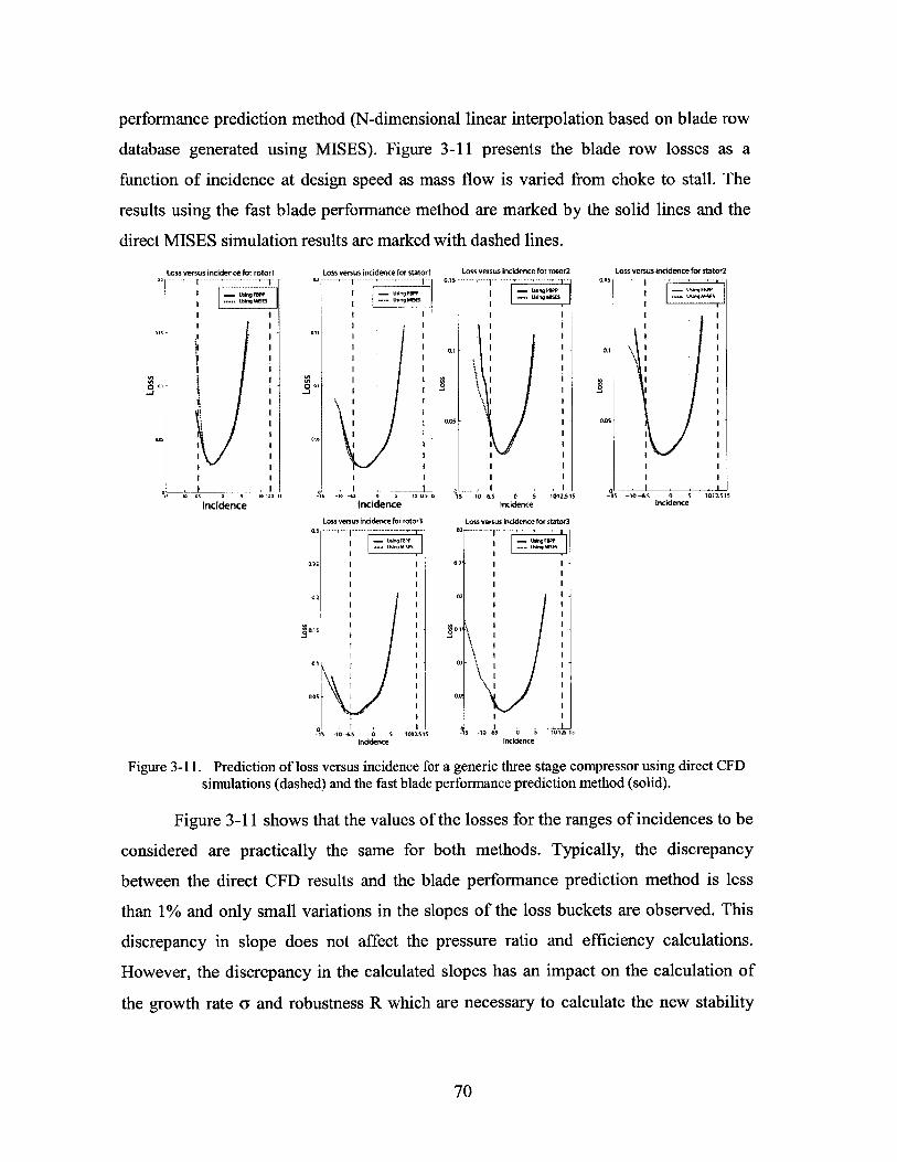
performance prediction method (N-dimensional linear interpolation based on blade row
database generated using MISES). Figure 3-11 presents the blade row losses as a
function of incidence at design speed as mass flow is varied from choke to stall. The
results using the fast blade performance method are marked by the solid lines and the
direct MISES simulation results are marked with dashed lines.
Loss versus incidence for rotor I
...... UsinhV ss
$AI
011
-is 1 s1 o S o s 2
Incidence
O0
0.
0.~
Loss versus incidence for statori
DI . ...... .. .
I Ii
I1 1 -S 0 1 .I l
15 I
0 I I
incidence
0.15Loss versus incidence for rotor2
F I
s -10-.S 0 5 1012.51!Incidence
Loss versus incidence for stator3
3 ----------------------------
Incidence
Loss versus incidence for stator2
0.1
*sI s
-1is -10-.s 0 o 1012.sisIncidence
Figure 3-11. Prediction of loss versus incidence for a generic three stage compressor using direct CFDsimulations (dashed) and the fast blade performance prediction method (solid).
Figure 3-11 shows that the values of the losses for the ranges of incidences to be
considered are practically the same for both methods. Typically, the discrepancy
between the direct CFD results and the blade performance prediction method is less
than 1% and only small variations in the slopes of the loss buckets are observed. This
discrepancy in slope does not affect the pressure ratio and efficiency calculations.
However, the discrepancy in the calculated slopes has an impact on the calculation of
the growth rate a and robustness R which are necessary to calculate the new stability
70
0
0
0
0.
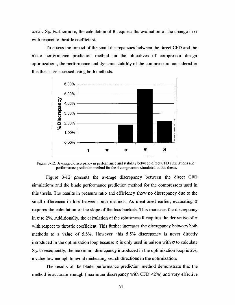
metric SD. Furthermore, the calculation of R requires the evaluation of the change in a
with respect to throttle coefficient.
To assess the impact of the small discrepancies between the direct CFD and the
blade performance prediction method on the objectives of compressor design
optimization , the performance and dynamic stability of the compressors considered in
this thesis are assessed using both methods.
6.00% -
5.00% -
Uc 4.00%-0.2 3.00%-
O 2.00% -
1.00% -
0.00% -
r r a R S
Figure 3-12. Averaged discrepancy in performance and stability between direct CFD simulations andperformance prediction method for the 4 compressors simulated in this thesis.
Figure 3-12 presents the average discrepancy between the direct CFD
simulations and the blade performance prediction method for the compressors used in
this thesis. The results in pressure ratio and efficiency show no discrepancy due to the
small differences in loss between both methods. As mentioned earlier, evaluating a
requires the calculation of the slope of the loss buckets. This increases the discrepancy
in a to 2%. Additionally, the calculation of the robustness R requires the derivative of a
with respect to throttle coefficient. This further increases the discrepancy between both
methods to a value of 5.5%. However, this 5.5% discrepancy is never directly
introduced in the optimization loop because R is only used in unison with a to calculate
SD. Consequently, the maximum discrepancy introduced in the optimization loop is 2%,
a value low enough to avoid misleading search directions in the optimization.
The results of the blade performance prediction method demonstrate that the
method is accurate enough (maximum discrepancy with CFD <2%) and very effective
71

(100 times faster than MISES) and is used to estimate the blade row performances in
the compressor design optimization framework.
72
Chapter 4
Compressor Design Optimization of aGeneric 3 Stage Compressor
The objective of this chapter is to implement and to apply the compressor design
optimization framework to a 3 stage baseline compressor. The goal is to demonstrate, as
conjectured in Chapters 1 and 2, that a performance improvement can be obtained if
dynamic stability is used as a prime design variable in the compressor design
optimization framework. This chapter is organized in four sections. First, previous
compressor optimization efforts are discussed and the advantages of the new approach
are described. Then, the inputs, outputs, assumptions and limitations of the different
modules used in the compressor design optimization framework are introduced. Next,
the 3 stage test compressor is defined and the baseline compressor performance and
stability are evaluated at different operating speeds. The new compressor design
optimization framework is then applied to the 3 stage compressor using two different
optimization strategies. The objective of the first optimization strategy is to improve the
compressor efficiencies at high speeds where a low specific fuel consumption is
desired. The second optimization strategy has the purpose to enhance the compressor
dynamic stability to improve the matching of the compressor stages at design and off-
design conditions.
4.1 Previous Work
The compressor design optimization framework developed and used in this
thesis is based on Perrot's [21] framework. Perrot used surge margin as one of the prime
design objectives and demonstrates a 6% improvement in surge margin at design
conditions at the cost of a 0.5% drop in efficiency and a 2% decrease in pressure ratio
73
for a 3 stage compressor. The new optimization framework improves Perrot's work in
several aspects. Instead of a single point optimization the new framework allows the
design optimization across the entire compressor map, i.e. objectives functions can be
specified at various speeds, to tailor and to improve the matching of the compressor
stages at design and off-design operating conditions. Additionally, the new blade
performance prediction method (see Chapter 3 for details) is capable to efficiently
predict the blade performance as a function of multiple blade geometric parameters (7
used in this thesis) compared to only 1 parameter in Perrot's formulation. This
introduces more freedom in the search for the optimal blade row and compressor
configuration which potentially could enable enhanced compressor performance and
operability. Furthermore, the new compressor design optimization framework is based
on dynamic stability and uses the new metric SD to assess stability. This offers to further
improve compressor performance as illustrated in Chapters 1 and 2.
4.2 Novel Compressor Design Optimization Framework
The compressor design optimization framework consists of three modules: the
optimization module, the fast blade performance prediction module and the compressor
flow field simulation module. The optimizer assesses if the user defined objectives and
constraints are satisfied. The objective of the optimization is to define the desired
attributes of the compressor to be optimized and thus represent the design philosophy to
be used. If the objectives and constraints are not met, the optimizer modifies the
compressor geometry and tries to provide an improved compressor design. Then, the
compressor flow field simulation code evaluates the performance and stability of the
new compressor geometry throughout the operating envelope. In order to calculate the
compressor performance and stability the performance of the individual blade rows
needs to be predicted. Consequently, the fast blade performance prediction method is
used together with the flow field simulation code to calculate the compressor
performance and stability. Finally, if the optimization objectives and constraints are
satisfied the optimal compressor design is obtained. Otherwise, the optimization loop is
repeated until the final optimal design is reached.
74
The inputs, assumptions and limitations of the compressor design optimization
framework modules are described next.
4.2.1 Compressor Flow Field Simulation Code
The flow field simulation code is divided into two parts: a mean-line flow
calculation and a dynamic stability calculation. A similar mean-line flow solver was
previously used by Dorca [7] and Perrot [21]. It calculates the compressor performance
in terms of overall pressure ratio and adiabatic efficiency and the uniform time-mean
flow field quantities that are required to compute the unsteady flow field perturbations
and dynamic stability. The inputs to the mean-line flow solver are:
* Number of compressor stages
e Hub and tip radii for each blade row
" Compressor inlet conditions (temperature and pressure)
" Compressor inlet mass flow
* rotor speed
" Blade row and gas path geometry (y, X1, X2, a, c, tm and xm for each of
blade rows).
The mean-line flow calculation neglects 3D loss effects. This limits the
application of the mean-line flow solver to compressor stages with high hub-to-tip
radius ratios. In addition, the deviation effects are accounted for using empirical
correlations valid for operating conditions near zero incidence operation.
Using the steady background flow field from the mean-line calculation and
blade row loss characteristics the dynamic compressor stability model computes the
compressor pre-stall modes, or natural frequencies of the flow field perturbations. The
growth rate a of the least stable mode is determined to calculate R and SD as discussed
in Chapter 2. More specifically, the inputs to the dynamic compressor stability model
are:
e Number of compressor stages
" Axial chord length of each of the blade rows, inlet and outlet duct
lengths and inter blade-row gap lengths
75
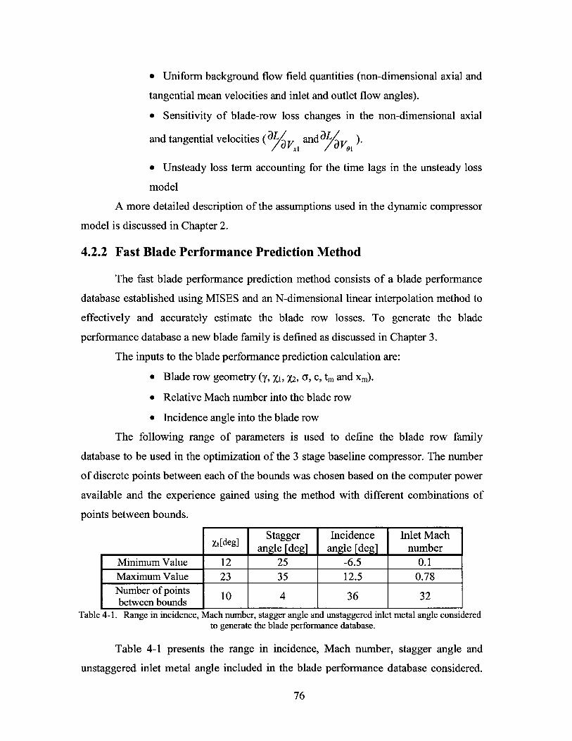
e Uniform background flow field quantities (non-dimensional axial and
tangential mean velocities and inlet and outlet flow angles).
* Sensitivity of blade-row loss changes in the non-dimensional axial
and tangential velocities (aL anda V
* Unsteady loss term accounting for the time lags in the unsteady loss
model
A more detailed description of the assumptions used in the dynamic compressor
model is discussed in Chapter 2.
4.2.2 Fast Blade Performance Prediction Method
The fast blade performance prediction method consists of a blade performance
database established using MISES and an N-dimensional linear interpolation method to
effectively and accurately estimate the blade row losses. To generate the blade
performance database a new blade family is defined as discussed in Chapter 3.
The inputs to the blade performance prediction calculation are:
e Blade row geometry (y, X, X2, a, c, tm and xm).
e Relative Mach number into the blade row
* Incidence angle into the blade row
The following range of parameters is used to define the blade row family
database to be used in the optimization of the 3 stage baseline compressor. The number
of discrete points between each of the bounds was chosen based on the computer power
available and the experience gained using the method with different combinations of
points between bounds.
Stagger Incidence Inlet MachI lgdeg] aIagle [deg] Iangle [deg] I number
Minimum Value 12 25 -6.5 0.1Maximum Value 23 35 12.5 0.78Number of points 10 4 36 32between bounds I I I I
Table 4-1. Range in incidence, Mach number, stagger angle and unstaggered inlet metal angle consideredto generate the blade performance database.
Table 4-1 presents the range in incidence, Mach number, stagger angle and
unstaggered inlet metal angle included in the blade performance database considered.
76
Other parameters such as gas path radii, chord length, and solidity can be included
without major implementation but for simplicity only Mach number, incidence, stagger
angle and unstaggered inlet metal angle were varied in the cases investigated.
4.2.3 Optimizer
This section describes the algorithm used by the optimizer and the optimization
problem set-up (i.e. objective functions and constraints) required to start the
optimization tool.
4.2.3.1 Algorithm
A gradient-based method is used to search the design space for an optimal
compressor design. Specifically, the sequential quadratic programming algorithm (SQP)
implemented in Matlab's optimization toolbox is used (fiincon function). At the start
of each optimization loop, gradient-based search methods use the information in the
gradient matrix to obtain a new search direction that maximizes the user defined
objective function and satisfies the constraints of the optimization problem.
The SQP algorithm is widely used in engineering applications and is adequate
for constrained and non-linear optimization problems. This is well-suited for the highly
constrained compressor design optimization because the operating incidences need to be
within the incidence bounds set by the blade performance prediction method and some
minimum requirements in pressure ratio, efficiency and stability need be satisfied.
Also, the sequential quadratic programming algorithm is appropriate for the
compressor design optimization because the relationship between geometry,
performance and dynamic stability is non-linear (for more details on the principles of
the SQP algorithm see Willcox [25]).
Three inputs are provided to the SQP algorithm: the objective function (i.e.
pressure ratio, efficiency or stability), the independent variables (i.e. compressor
geometry) and the optimization constraints (i.e. minimum requirements for the objective
function and incidence bounds).
77
4.2.3.2 Objective Function Used in the Compressor Design Optimization
Depending on the compressor design philosophy, the compressor optimization
objectives might be set up differently. For example, over the past four decades
designing for maximum efficiency has been the driver of most compressor design
optimizations (Greitzer and Wisler [11]). In the compressor optimizations for maximum
efficiency one would want to optimize for maximum efficiency at high speeds where
low specific fuel consumption is desired. Additionally, current compressor design
efforts are also geared towards the reduction of compressor flow field instabilities
throughout the operating envelope. Thus, one might also want to optimize for maximum
stability at design and off-design operating conditions to ensure the adequate matching
of the compressor stages and to avoid the use of variable geometries and bleed valves.
Since the compressor design philosophy is case dependent, a versatile objective
function representing the most relevant design philosophies (i.e. enhancing pressure
ratio, efficiency and stability) is created. In particular, the compressor geometry can be
optimized for maximum pressure ratio, stability or efficiency at one or several operating
speeds. Weighting factors ( ) can be assigned to each of the objectives at the different
operating conditions. This favors improvements in the compressor design in the
operating regions of interest. Furthermore, one can create an objective function
including any weighted (p) combination of the previous objective functions. This
objective function is in general of the form:
OBJ=p,x lis,,d ISpeed +P,,X ZJe, 7speed +PS X Epeed SDSpeed 1
Speed TiSpeed Speed 1iSpeed Speed SDiSpeed
where all the objectives are normalized by their baseline values, is the weighting
factor assigned to the individual objectives at different speeds and p is the weighting
factor used for the compounded sum of the pressure ratio, efficiency and dynamic
stability objective functions.
4.2.3.3 Constraints of the Compressor Design Optimization
Constraints are used to ensure that the operating incidences are within the
incidence bounds where the fast blade performance prediction method generates
78
accurate results. As discussed in Chapter 3, this is important because a small
discrepancy in the compressor performance and stability calculations at the start of the
compressor design optimization process might lead to sub-optimal compressor
geometries. In addition, constraints are included to guarantee a certain minimum level
of efficiency and stability across the operating envelope. Finally, bounds on the
operating line in terms of the maximum and minimum working line pressure ratio are
included to ensure that the demands of the turbine are satisfied.
4.2.3.4 Independent Variables of the Compressor Design Optimization
The variables of the compressor optimization problem are the absolute exit
metal angle of the IGV upstream of rotor 1 and the geometric parameters required to
generate the blade row geometries and the gas flow path. For simplicity, in this thesis
only the exit metal angle of the fixed geometry IGV, the stagger angle and unstaggered
inlet metal angles of the individual blade rows are introduced as independent variable.
Thus, the optimization problems of the 3 stage baseline compressor considered in this
thesis includes 13, independent variables (2 x 6+1).
4.3 Baseline 3 Stage Compressor
The baseline compressor geometry used in this thesis is designed such that the
compressor stability remains constant throughout the operating envelope. As discussed
in Cumpsty [5], this can be achieved by setting the incidences at design speed to
negative values in the front stages and to positive values in the rear stages since, as the
operating speed is reduced from design speed, the flow coefficients along the
compressor change. The result of a reduced operating speed is that the front stage
operating conditions shift towards positive incidences (or stall) and the rear stages
operating conditions shift towards negative incidences (or choking).
79
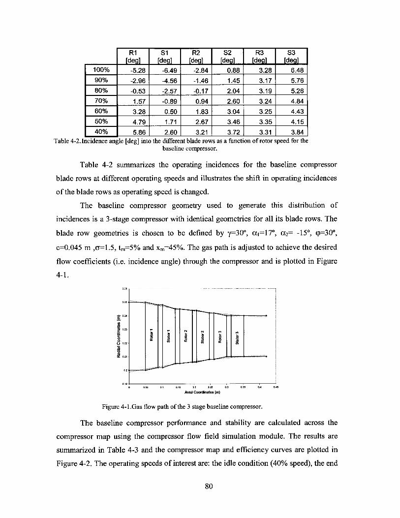
R1[deal
I I I U U
S1[deal
R2[deal
S2[degl
R3[degl
S3[degl
100% -5.28 -6.49 -2.84 0.88 3.28 6.48
90% -2.96 -4.56 -1.46 1.45 3.17 5.76
80% -0.53 -2.57 -0.17 2.04 3.19 5.2670% 1.57 -0.89 0.94 2.60 3.24 4.84
60% 3.28 0.50 1.83 3.04 3.25 4.43
50% 4.79 1.71 2.67 3.46 3.35 4.15
40% 5.86 2.60 3.21 3.72 3.31 3.84Table 4-2. Incidence angle [deg] into the different blade rows as a function of rotor speed for the
baseline compressor.
Table 4-2 summarizes the operating incidences for the baseline compressor
blade rows at different operating speeds and illustrates the shift in operating incidences
of the blade rows as operating speed is changed.
The baseline compressor geometry used to generate this distribution of
incidences is a 3-stage compressor with identical geometries for all its blade rows. The
blade row geometries is chosen to be defined by y= 3 0*, c1=17 0, a 2= -15*, <p=30 0,
c=0.045 m ,r=1.5, tm=5% and xm=45%. The gas path is adjusted to achieve the desired
flow coefficients (i.e. incidence angle) through the compressor and is plotted in Figure
4-1.
..2 .....
0 C
0 005 01 010 02 025 0.3 0.s 04 0A5Axial Coordinates (m)
Figure 4-1.Gas flow path of the 3 stage baseline compressor.
The baseline compressor performance and stability are calculated across the
compressor map using the compressor flow field simulation module. The results are
summarized in Table 4-3 and the compressor map and efficiency curves are plotted in
Figure 4-2. The operating speeds of interest are: the idle condition (40% speed), the end
80
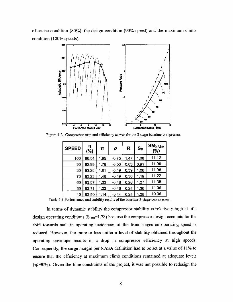
of cruise condition (80%), the design condition (90% speed) and the maximum climb
condition (100% speeds).m | 2.s
/
a,
o.-
2
Iis
1,--- 402 4 6 S 10 12 14 0 5 10 is
Corrected Mass Flow Corrected Mass Flow
Figure 4-2. Compressor map and efficiency curves for the 3 stage baseline compressor.
SPEED '1 Tr a R SD SMNASA
100 90.54 1.95 -0.75 1.47 1.08 11.12
90 92.89 1.78 -0.50 0.63 0.91 11-09
80 93.26 1.61 -0.49 0.39 1.06 11.08
70 93.23 1.46 -0.49 0.30 1.19 11.22
60 93.07 1.33 -0.48 0.26 1.27 11.38
50 92.71 1.22 -0.46 0.24 1.30 11.06
40 92.50 1.14 -0.44 0.24 1.28 10.06
Table 4-3.Performance and stability results of the baseline 3-stage compressor.
In terms of dynamic stability the compressor stability is relatively high at off-
design operating conditions (SD40=1.28) because the compressor design accounts for the
shift towards stall in operating incidences of the front stages as operating speed is
reduced. However, the more or less uniform level of stability obtained throughout the
operating envelope results in a drop in compressor efficiency at high speeds.
Consequently, the surge margin per NASA definition had to be set at a value of 11% to
ensure that the efficiency at maximum climb conditions remained at adequate levels
(TI>90%). Given the time constraints of the project, it was not possible to redesign the
81
/
so
70a.m [
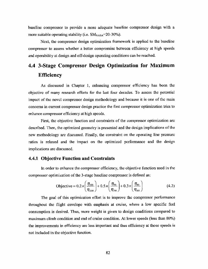
baseline compressor to provide a more adequate baseline compressor design with a
more suitable operating stability (i.e. SMNASA=20- 3 0%).
Next, the compressor design optimization framework is applied to the baseline
compressor to assess whether a better compromise between efficiency at high speeds
and operability at design and off-design operating conditions can be reached.
4.4 3-Stage Compressor Design Optimization for Maximum
Efficiency
As discussed in Chapter 1, enhancing compressor efficiency has been the
objective of many research efforts for the last four decades. To assess the potential
impact of the novel compressor design methodology and because it is one of the main
concerns in current compressor design practice the first compressor optimization tries to
enhance compressor efficiency at high speeds.
First, the objective function and constraints of the compressor optimization are
described. Then, the optimized geometry is presented and the design implications of the
new methodology are discussed. Finally, the constraint on the operating line pressure
ratios is relaxed and the impact on the optimized performance and the design
implications are discussed.
4.4.1 Objective Function and Constraints
In order to enhance the compressor efficiency, the objective function used in the
compressor optimization of the 3-stage baseline compressor is defined as:
Objective = 0.2x r o +0.5x r ) +0.3x r-!9-i (4.2)K"100 )+ J !Ei9o /80
The goal of this optimization effort is to improve the compressor performance
throughout the flight envelope with emphasis at cruise, where a low specific fuel
consumption is desired. Thus, more weight is given to design conditions compared to
maximum climb condition and end of cruise condition. At lower speeds (less than 80%)
the improvements in efficiency are less important and thus efficiency at those speeds is
not included in the objective function.
82
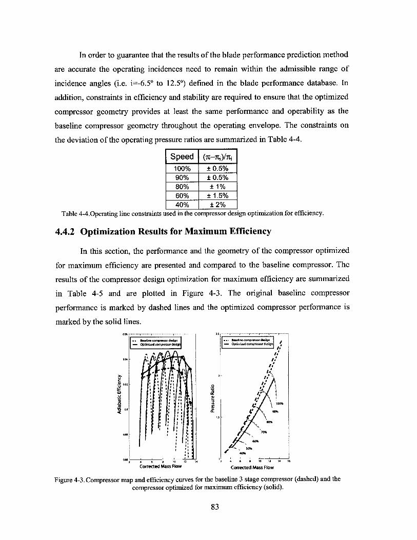
In order to guarantee that the results of the blade performance prediction method
are accurate the operating incidences need to remain within the admissible range of
incidence angles (i.e. i=-6.5* to 12.50) defined in the blade performance database. In
addition, constraints in efficiency and stability are required to ensure that the optimized
compressor geometry provides at least the same performance and operability as the
baseline compressor geometry throughout the operating envelope. The constraints on
the deviation of the operating pressure ratios are summarized in Table 4-4.
Speed (n-7i)/i100% ± 0.5%90% ± 0.5%80% ±1%60% 1.5%40% ±2%
Table 4-4.Operating line constraints used in the compressor design optimization for efficiency.
4.4.2 Optimization Results for Maximum Efficiency
In this section, the performance and the geometry of the compressor optimized
for maximum efficiency are presented and compared to the baseline compressor. The
results of the compressor design optimization for maximum efficiency are summarized
in Table 4-5 and are plotted in Figure 4-3. The original baseline compressor
performance is marked by dashed lines and the optimized compressor performance is
marked by the solid lines.0 9 --- --6 i- -- ---- r-- --- --I- -- ---- .5 --- --- -- ----I- -- --- ---- --I- --- -- --- --
FigurB4-p an e sin caseline 3 compr essor design(
omzdcompressor e ptimized frm x um e icimecyr (sid.'
0.9 *
I L2 0 12 1 6 a 0 1 4 1
Corce Mas FlwCrete2asFo
Fiur 43.Coprssr apan efiiecycuve fr hebaelne3 tae omreso (ase.92d h
copeso opiie for. maiu. ffcec(oi)
83
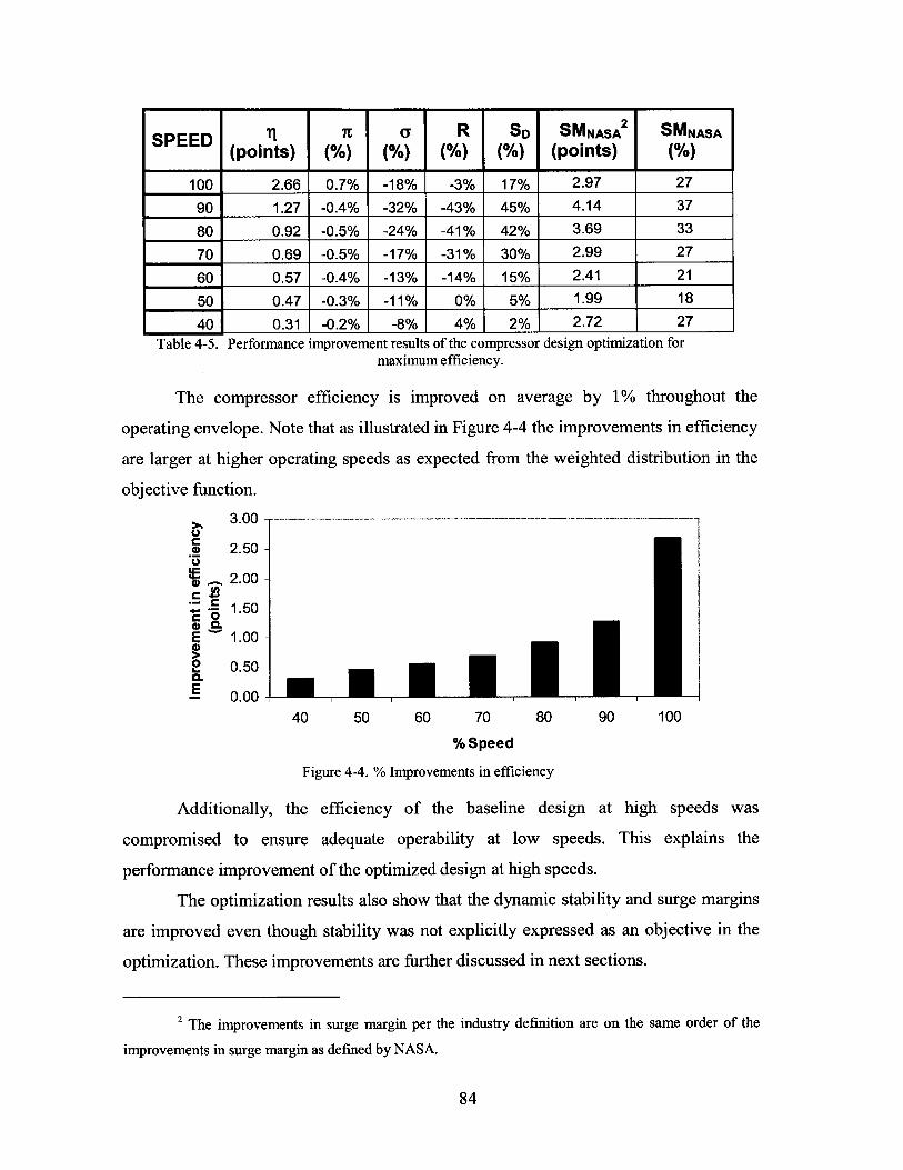
SPEED a R SD SMNASA 2 SMNASA(points) (%) (%) (%) (%) (points) (%)
100 2.66 0.7% -18% -3% 17% 2.97 27
90 1.27 -0.4% -32% -43% 45% 4.14 37
80 0.92 -0.5% -24% -41% 42% 3.69 33
70 0.69 -0.5% -17% -31% 30% 2.99 27
60 0.57 -0.4% -13% -14% 15% 2.41 21
50 0.47 -0.3% -11% 0% 5% 1.99 18
40 0.31 -0.2% -8% 4% 2% 2.72 27
Table 4-5. Performance improvement results of the compressor design optimization formaximum efficiency.
The compressor efficiency is improved on average by 1% throughout the
operating envelope. Note that as illustrated in Figure 4-4 the improvements in efficiency
are larger at higher operating speeds as expected from the weighted distribution in the
objective function.
3.00CCD 2.50 -
2.00-
1.50-CL
E 1.00-
02. 0.50-0.E 0.00
40 50 60 70 80 90 100
% Speed
Figure 4-4. % Improvements in efficiency
Additionally, the efficiency of the baseline design at high speeds was
compromised to ensure adequate operability at low speeds. This explains the
performance improvement of the optimized design at high speeds.
The optimization results also show that the dynamic stability and surge margins
are improved even though stability was not explicitly expressed as an objective in the
optimization. These improvements are further discussed in next sections.
2 The improvements in surge margin per the industry definition are on the same order of the
improvements in surge margin as defined by NASA.
84
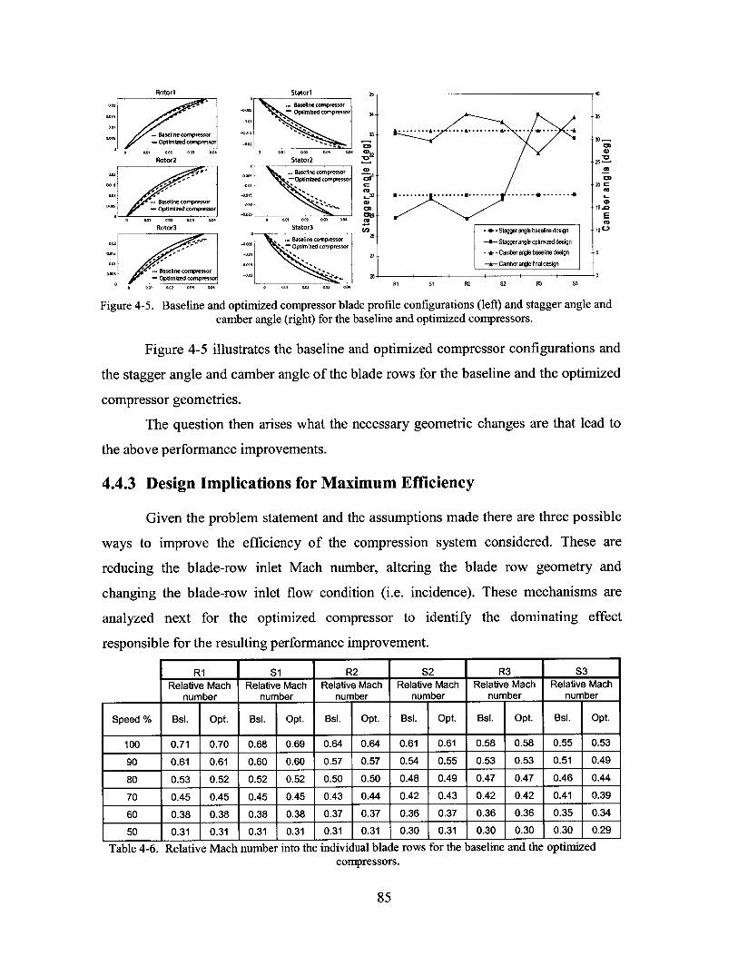
Rotor1 Stator1 35 40
0.02 ... Bseline compressor
oms.. Optimized compressor
Baseline compressor -Ba i 33-- Optimized compressor -04 3
S0.01 0.02 0.03 o0 0 a0 002 004 oM 0 0Rotor2 Stator2 25
0.02 Baseline compressoroOptemszed compressor
*15 -0o01 2o C
Rotor3- Stator - tge agebsieUein t
om , - -01+-Cabragl1aenedsg
Baseline compressor 0- Optimized compressor - 215.0
0 0 01 0 O2 0 004 -002 0.02 0M 0E R1 S3000r~ 001or 002 U 0
Ra0r Sttr 28 -w - Stagger angle baseline design s.
00r 4- B s i andopti i . line compressor a n tagger angle optandad designca m Optitized compressor
Figure -0.01 h b n Camber angle baselne design n50t01 s g ansge -an-Camber angle final design
co e Baseline ompressor01 Optimized compressor -00 N ~ 3
0 0.01 0-02 003 0504 D 0101 0,02 04 004 R1 51 R2 S2 R3 S3
Figure 4-5. Baseline and optimized compressor blade profile configurations (left) and stagger angle andcamber angle (right) for the baseline and optim-ized compressors.
Figure 4-5 illustrates the baseline and optimized compressor configurations and
the stagger angle and camber angle of the blade rows for the baseline and the optimized
compressor geometries.
The question then arises what the necessary geometric changes are that lead to
the above performance improvements.
4.4.3 Design Implications for Maximum Efficiency
Given the problem statement and the assumptions made there are three possible
ways to improve the efficiency of the compression system considered. These are
reducing the blade-row inlet Mach number, altering the blade row geometry and
changing the blade-row inlet flow condition (i.e. incidence). These mechanisms are
analyzed next for the optimized compressor to identify the dominating effect
responsible for the resulting performance improvement.
R1 S1 R2 S2 R3 S3Relative Mach Relative Mach Relative Mach Relative Mach Relative Mach Relative Mach
number number number number number number
Speed % Bsl. Opt. BsI. Opt. Bsl. Opt. Bsl. Opt. Bsl. Opt. Bsl. Opt.
100 0.71 0.70 0.68 0.69 0.64 0.64 0.61 0.61 0.58 0.58 0.55 0.53
90 0.61 0.61 0.60 0.60 0.57 0.57 0.54 0.55 0.53 0.53 0.51 0.49
80 0.53 0.52 0.52 0.52 0.50 0.50 0.48 0.49 0.47 0.47 0.46 0.44
70 0.45 0.45 0.45 0.45 0.43 0.44 0.42 0.43 0.42 0.42 0.41 0.39
60 0.38 0.38 0.38 0.38 0.37 0.37 0.36 0.37 0.36 0.36 0.35 0.34
50 0.31 0.31 0.31 0.31 0.31 0.31 0.30 0.31 0.30 0.30 0.30 0.29
Table 4-6. Relative Mach number into the individual blade rows for the baseline and the optimizedcompressors.
85
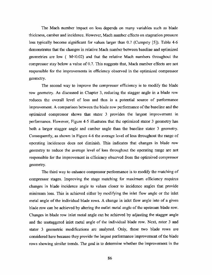
The Mach number impact on loss depends on many variables such as blade
thickness, camber and incidence. However, Mach number effects on stagnation pressure
loss typically become significant for values larger than 0.7 (Cumpsty [5]). Table 4-6
demonstrates that the changes in relative Mach number between baseline and optimized
geometries are low ( M<0.02) and that the relative Mach numbers throughout the
compressor stay below a value of 0.7. This suggests that, Mach number effects are not
responsible for the improvements in efficiency observed in the optimized compressor
geometry.
The second way to improve the compressor efficiency is to modify the blade
row geometry. As discussed in Chapter 3, reducing the stagger angle in a blade row
reduces the overall level of loss and thus is a potential source of performance
improvement. A comparison between the blade row performance of the baseline and the
optimized compressor shows that stator 3 provides the largest improvement in
performance. However, Figure 4-5 illustrates that the optimized stator 3 geometry has
both a larger stagger angle and camber angle than the baseline stator 3 geometry.
Consequently, as shown in Figure 4-6 the average level of loss throughout the range of
operating incidences does not diminish. This indicates that changes in blade row
geometry to reduce the average level of loss throughout the operating range are not
responsible for the improvement in efficiency observed from the optimized compressor
geometry.
The third way to enhance compressor performance is to modify the matching of
compressor stages. Improving the stage matching for maximum efficiency requires
changes in blade incidence angle to values closer to incidence angles that provide
minimum loss. This is achieved either by modifying the inlet flow angle or the inlet
metal angle of the individual blade rows. A change in inlet flow angle into of a given
blade row can be achieved by altering the outlet metal angle of the upstream blade row.
Changes in blade row inlet metal angle can be achieved by adjusting the stagger angle
and the unstaggered inlet metal angle of the individual blade row. Next, rotor 3 and
stator 3 geometric modifications are analyzed. Only, these two blade rows are
considered here because they provide the largest performance improvement of the blade
rows showing similar trends. The goal is to determine whether the improvement in the
86
matching of the compressor stages is due to the modification of the inlet flow angles,
the inlet metal angles or both.100 % Speed 90 % Speed 80 % Speed
0.15 0.15 0.15
0.1 $. 010 ~ 0 0
0.0s . 0.05 J 005
0 0-10 -5 0 5 10 15 -10 -5 0dd 5 10 15 -10 -5 0 5 10 15Incidence Incidence Incidence
70 % Speed 60 % Speed 50 % Speed
0.15 0.15 0.15
qA 0.1 0.1 1 0.1o0 0 0
0.05 0.05 g 0.05
0 -- -- 0 0 ___j --10 -5 0 5 10 15 -10 -5 0 5 10 5 -10 5 0 5 10 15
Incidence Incidence Incidence40 % Speed f.Mc ub
Baseline compressor design Baseline Opmized-Optimized ompressor design
0.1%A 0.1~ L o 050 .80
-. 7 0.4072 0.390.05 60 10.354 0.34
-. 05Stator 3-10 -5 0 5 10 15
Incidence
Figure 4-6. Loss buckets for stator 3 for the baseline compressor (dashed) and the optimized compressorgeometry (solid) at different operating speeds. Working line operating points are marked by circles
Figure 4-6 depicts the loss buckets at different speeds for stator 3 and illustrates
the shift in operating incidence to values closer to the incidence at minimum loss. As
illustrated in Figure 4-5, camber angle and stagger angle of the third stator blade are
both increased. This indicates that the inlet metal angle is increased (+5.6550). In
addition, the stagger angle of rotor 3 is increased by 3.9740 thus yielding a larger outlet
metal angle. The larger outlet flow angle of rotor 3 implies a decrease in inlet flow
angle to stator 3(-3.9740). Thus, both the increase in inlet metal angle of the blade row
and the increase in outlet metal angle of the blade row upstream are responsible for the
improvement in compressor stages matching. For the third stator blade row these
changes in geometry result in a total reduction in operating incidence of 9.630.
The enhanced stability for the optimized compressor at high speeds can be
attributed to the improvement in compressor matching. In the baseline case stator 3 is
operating at positive incidences on the stall side of the loss bucket at high speeds. The
optimization process reduces the operating incidence and shifts the operating points
closer to the choke side. This increases the operating range and thus enhances the
87
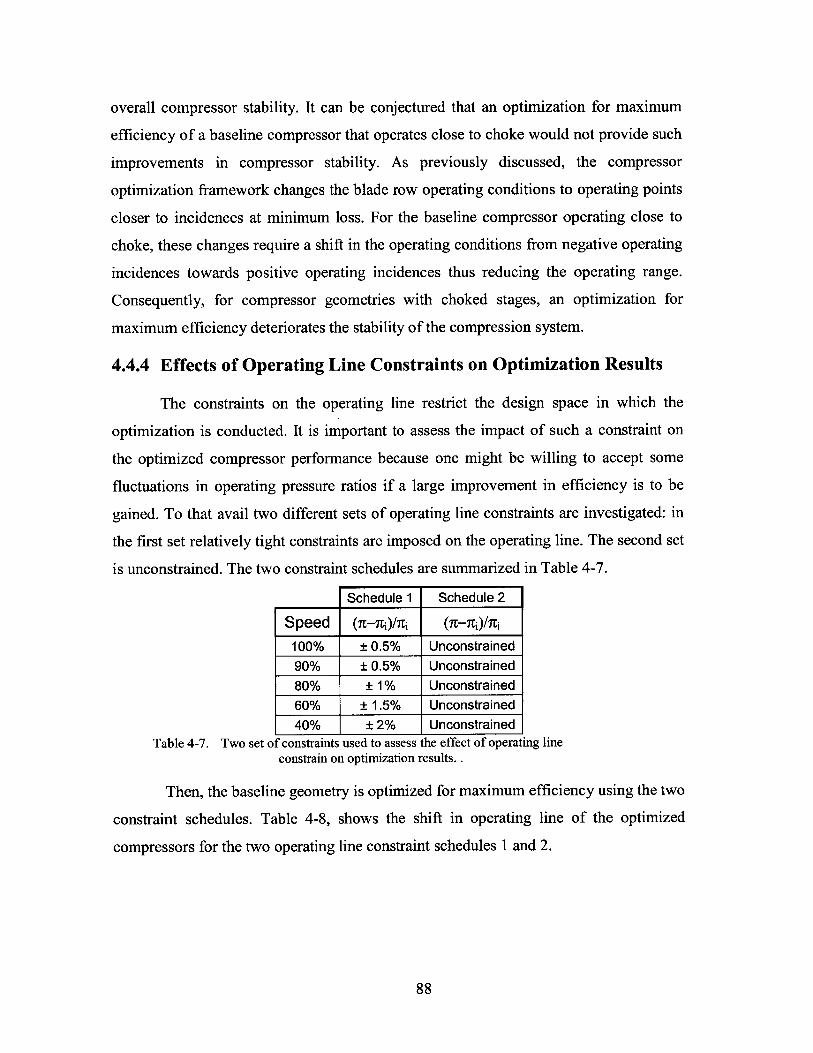
overall compressor stability. It can be conjectured that an optimization for maximum
efficiency of a baseline compressor that operates close to choke would not provide such
improvements in compressor stability. As previously discussed, the compressor
optimization framework changes the blade row operating conditions to operating points
closer to incidences at minimum loss. For the baseline compressor operating close to
choke, these changes require a shift in the operating conditions from negative operating
incidences towards positive operating incidences thus reducing the operating range.
Consequently, for compressor geometries with choked stages, an optimization for
maximum efficiency deteriorates the stability of the compression system.
4.4.4 Effects of Operating Line Constraints on Optimization Results
The constraints on the operating line restrict the design space in which the
optimization is conducted. It is important to assess the impact of such a constraint on
the optimized compressor performance because one might be willing to accept some
fluctuations in operating pressure ratios if a large improvement in efficiency is to be
gained. To that avail two different sets of operating line constraints are investigated: in
the first set relatively tight constraints are imposed on the operating line. The second set
is unconstrained. The two constraint schedules are summarized in Table 4-7.
Schedule 1 Schedule 2
Speed (nc-Li)/ni (n-7ti)/7i
100% ± 0.5% Unconstrained90% +0.5% Unconstrained80% ± 1% Unconstrained60% +1.5% Unconstrained40% ± 2% Unconstrained
Table 4-7. Two set of constraints used to assess the effect of operating lineconstrain on optimization results. .
Then, the baseline geometry is optimized for maximum efficiency using the two
constraint schedules. Table 4-8, shows the shift in operating line of the optimized
compressors for the two operating line constraint schedules 1 and 2.
88
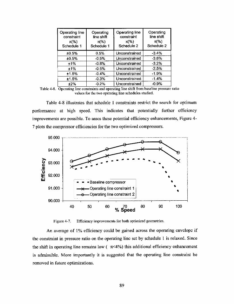
Operating line Operating Operating line Operatingconstraint line shift constraint line shift
R(%) R(%) n(%) n(%)Schedule 1 Schedule 1 Schedule 2 Schedule 2
±0.5% 0.5% Unconstrained -3.4%±0.5% -0.5% Unconstrained -3.8%
±1% -0.6% Unconstrained -3.2%±1% -0.5% Unconstrained -2.5%
±1.5% -0.4% Unconstrained -1.9%±1.5% -0.3% Unconstrained -1.4%±2% -0.2% Unconstrained -0.9%
Table 4-8. Operating line constraints and operating line shift from baseline pressure ratiovalues for the two operating line schedules studied.
Table 4-8 illustrates that schedule 1 constraints restrict the search for optimum
performance at high speed. This indicates that potentially further efficiency
improvements are possible. To asses these potential efficiency enhancements, Figure 4-
7 plots the compressor efficiencies for the two optimized compressors.
95.000 --------
94.000-
0 93.000-
92.000-- - - Baseline compressor
91.000- -x--Operating line constraint 1-e-Operating line constraint 2
90.000- 1 1 1
40 50 60 70 80 90 100% Speed
Figure 4-7. Efficiency improvements for both optimized geometries.
An average of 1% efficiency could be gained across the operating envelope if
the constraint in pressure ratio on the operating line set by schedule 1 is relaxed. Since
the shift in operating line remains low ( n<4%) this additional efficiency enhancement
is admissible. More importantly it is suggested that the operating line constraint be
removed in future optimizations.
89
4.5 Optimization for Maximum Stability
As discussed in Chapter 1, enhancing compressor operability across the
operating envelope is a major focus of current design efforts. The compressor design
optimization framework is applied to the 3-stage baseline compressor to investigate the
implications of a design for maximum dynamic stability and to assess the potential
impact of improvements in compressor matching throughout the operating envelope
without the use of bleed valves or variable stator geometries. The objective is to
enhance compressor stability and to do so two design philosophies are adopted. The
first philosophy optimizes for maximum dynamic stability at cruise while the second
philosophy also includes an stability objective at idle speed. First, the objective
functions and constraints of the two compressor optimizations are described. Then, the
optimized geometries are presented and the design implications of the new
methodology are discussed.
4.5.1 Objectives Functions and Constraints
In order to enhance compressor stability, two objective functions are used in the
compressor optimizations for maximum stability of the 3 stage baseline compressor:
OBJ1= -x D100 2 -XD70OB I ii)+x (4.3)3 SDil00 3 SDi70
1 S 1 S 1 SOBJ2= -x D10 I D90 (4.4)
4 KSDil00 2 (sDi90 )4 SDi4O
The goal of the first design optimization philosophy (Equation (4.3)) is to
improve the compressor stability at maximum climb conditions and at end of cruise
conditions. This will be compared to the second design philosophy for enhanced
operability which is aimed at improving the compressor stability at maximum climb
conditions, design conditions and also at idle conditions where engine accelerations and
low flow coefficients can trigger instability.
The constraints used in both compressor design optimization problems are
identical and are the same as used in the compressor design optimization for maximum
efficiency. These constraints are the incidence bounds on the operating
90
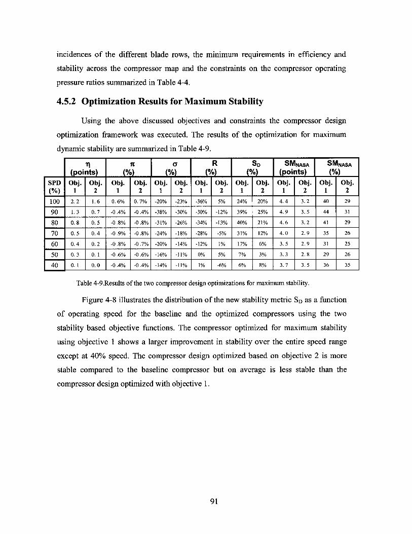
incidences of the different blade rows, the minimum requirements in efficiency and
stability across the compressor map and the constraints on the compressor operating
pressure ratios summarized in Table 4-4.
4.5.2 Optimization Results for Maximum Stability
Using the above discussed objectives and constraints the compressor design
optimization framework was executed. The results of the optimization for maximum
dynamic stability are summarized in Table 4-9.
I 2t a R SD SMNASA SMNASA(points % % (%) (%) (points) (%)
SPD Obj. Obj. Obj. Obj. Obj. Obj. Obj. Obj. Obj. Obj. Obj. Obj. Obj. Obj.(%) 1 2 1 2 1 2 1 2 1 2 1 2 1 2
100 2.2 1.6 0.6% 0.7% -20% -23% -36% 5% 24% 20% 4.4 3.2 40 29
90 1.3 0.7 -0 .4% -0.4% -38% -30% -30% -12% 39% 25% 4.9 3.5 44 31
80 0. 8 0. 5 -0 .8% -0.8% -31% -26% -34% -13% 40% 21% 4. 6 3.2 41 29
70 0.5 0.4 -0.9% -0.8% -24% -18% -28% -5% 31% 12% 4.0 2.9 35 26
60 0.4 0.2 -0 .8% -0.7% -20% -14% -12% 1% 17% 6% 3. 5 2. 9 31 25
50 0.3 0.1 -0.6% -0.6% -16% -11% 0% 5% 7% 3% 3.3 2.8 29 26
40 0. 1 0.0 -0.4% -0.4% -14% -11% 1% -6% 6% 8% 3.7 3.5 36 35
Table 4-9.Results of the two compressor design optimizations for maximum stability.
Figure 4-8 illustrates the distribution of the new stability metric SD as a function
of operating speed for the baseline and the optimized compressors using the two
stability based objective functions. The compressor optimized for maximum stability
using objective 1 shows a larger improvement in stability over the entire speed range
except at 40% speed. The compressor design optimized based on objective 2 is more
stable compared to the baseline compressor but on average is less stable than the
compressor design optimized with objective 1.
91
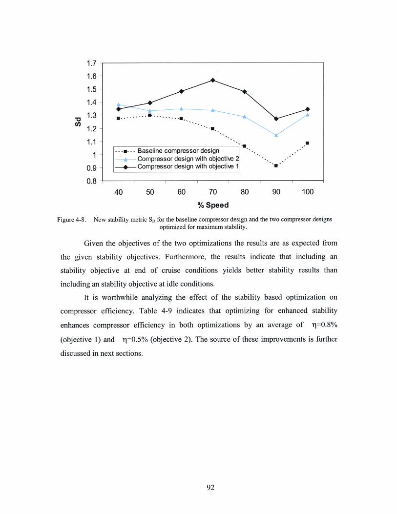
1.7 -
1.6 -
1.5 -
1.4-
1.2
1.1 - _'' U
1 - m- -- Baseline compressor designCompressor design with objective 2
0.9 - Compressor design with objective 1
0.8 1 1 1 1
40 50 60 70 80 90 100
%Speed
Figure 4-8. New stability metric SD for the baseline compressor design and the two compressor designsoptimized for maximum stability.
Given the objectives of the two optimizations the results are as expected from
the given stability objectives. Furthermore, the results indicate that including an
stability objective at end of cruise conditions yields better stability results than
including an stability objective at idle conditions.
It is worthwhile analyzing the effect of the stability based optimization on
compressor efficiency. Table 4-9 indicates that optimizing for enhanced stability
enhances compressor efficiency in both optimizations by an average of I=0.8%
(objective 1) and T1=0.5% (objective 2). The source of these improvements is further
discussed in next sections.
92
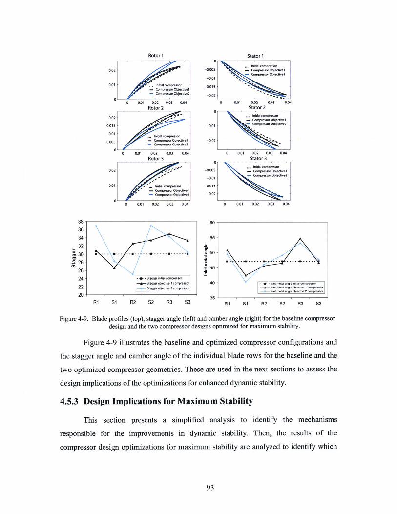
Rotor 1
... Initial compressorCompressor Objectivel
-Compressor Objective2
0.02
0.01
0
0.02
0.015
0.01
0.005
0
0.02
0.01
0
-0.005
-0.01
-0.015
-0.02
-0.01
-0.02
0-
-0.005
-0.01
-0.015
-0.02
0 0.01 0.02 0.03 0.04
- -------- -- U--- - - -. 4
- Stagger initial compressor-- Stagger objectie 1 compressor
Stagger objectie 2 compressor
R1 SI R2 S2 R3 S3
60
55-
m 50-
40 -
35
Stator 1
... Initial compressor. Compressor Objectivel--- Compressor Objective2
0.01 0.02 0.03 0.04Stator 2
... Initial compressor- Compressor Objectivel- Compressor Objective2
0 0.01 0.02 0.03 0.04
Stator 3
... Initial compressor- Compressor Objectivel1- Compressor Objective2
0 0.01 0.02 0.03 0.04
- - - Inlet metal angle initial compressor--- Inlet metal angle objectw 1 compressor
Inlet metal angle objectiw 2 compressor
R1 S1 R2 S2 R3 S3
Figure 4-9. Blade profiles (top), stagger angle (left) and camber angle (right) for the baseline compressordesign and the two compressor designs optimized for maximum stability.
Figure 4-9 illustrates the baseline and optimized compressor configurations and
the stagger angle and camber angle of the individual blade rows for the baseline and the
two optimized compressor geometries. These are used in the next sections to assess the
design implications of the optimizations for enhanced dynamic stability.
4.5.3 Design Implications for Maximum Stability
This section presents a simplified analysis to
responsible for the improvements in dynamic stability.
compressor design optimizations for maximum stability are
identify the mechanisms
Then, the results of the
analyzed to identify which
93
0 0.01 0.02 0.03 0.04
Rotor 2
Initial compressor. Compressor Objectivel- Compressor Objective2
0 0.01 0.02 0.03 0.04
Rotor 3
. Initial compressor
. Compressor Objectivel- Compressor Objective2
38
36
34
32
30
28
26
24
22
20
CO)
W-O I ihI11111111
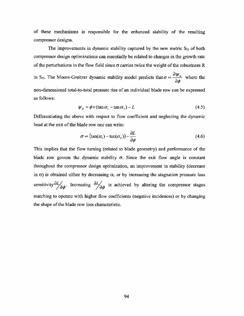
of these mechanisms is responsible for the enhanced stability of the resulting
compressor designs.
The improvements in dynamic stability captured by the new metric SD of both
compressor design optimizations can essentially be related to changes in the growth rate
of the perturbations in the flow field since a carries twice the weight of the robustness R
in SD. The Moore-Greitzer dynamic stability model predicts that a "V'aS where the
non-dimensional total-to-total pressure rise of an individual blade row can be expressed
as follows:
Y,,t = x (tan a, - tan a2) -L (4.5)
Differentiating the above with respect to flow coefficient and neglecting the dynamic
head at the exit of the blade row one can write:
aLa 0C (tan(a,) - tan(a 2 ))- (4.6)aob
This implies that the flow turning (related to blade geometry) and performance of the
blade row govern the dynamic stability a. Since the exit flow angle is constant
throughout the compressor design optimization, an improvement in stability (decrease
in a) is obtained either by decreasing a1 or by increasing the stagnation pressure loss
sensitivityaL . Increasing a is achieved by altering the compressor stages
matching to operate with higher flow coefficients (negative incidences) or by changing
the shape of the blade row loss characteristic.
94
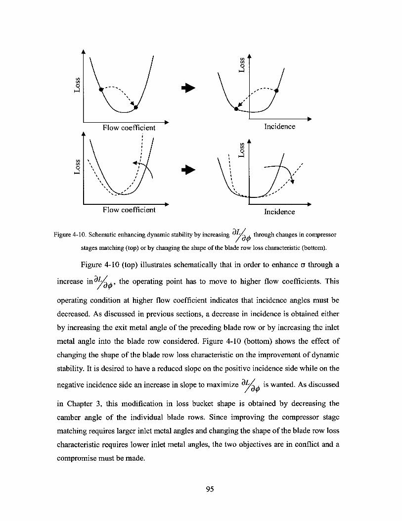
L
Flow coefficient Incidence
1.4 '
Flo cefict Incienc
Figure 4-10. Schematic enhancing dynamic stability by increasing through changes in compressor
stages matching (top) or by changing the shape of the blade row loss characteristic (bottom).
Figure 4-10 (top) illustrates schematically that in order to enhance a through a
increase in a , the operating point has to move to higher flow coefficients. This
operating condition at higher flow coefficient indicates that incidence angles must be
decreased. As discussed in previous sections, a decrease in incidence is obtained either
by increasing the exit metal angle of the preceding blade row or by increasing the inlet
metal angle into the blade row considered. Figure 4-10 (bottom) shows the effect of
changing the shape of the blade row loss characteristic on the improvement of dynamic
stability. It is desired to have a reduced slope on the positive incidence side while on the
negative incidence side an increase in slope to maximize 'JL is wanted. As discussed
in Chapter 3, this modification in loss bucket shape is obtained by decreasing the
camber angle of the individual blade rows. Since improving the compressor stage
matching requires larger inlet metal angles and changing the shape of the blade row loss
characteristic requires lower inlet metal angles, the two objectives are in conflict and a
compromise must be made.
95
A
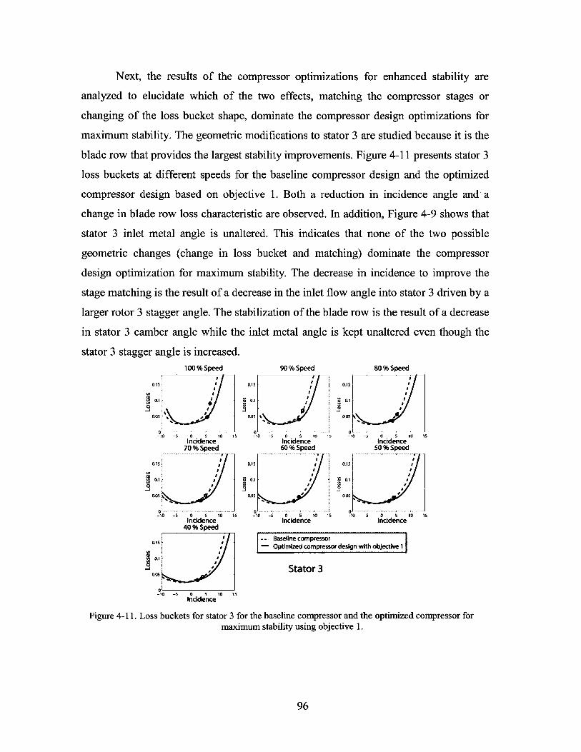
Next, the results of the compressor optimizations for enhanced stability are
analyzed to elucidate which of the two effects, matching the compressor stages or
changing of the loss bucket shape, dominate the compressor design optimizations for
maximum stability. The geometric modifications to stator 3 are studied because it is the
blade row that provides the largest stability improvements. Figure 4-11 presents stator 3
loss buckets at different speeds for the baseline compressor design and the optimized
compressor design based on objective 1. Both a reduction in incidence angle and a
change in blade row loss characteristic are observed. In addition, Figure 4-9 shows that
stator 3 inlet metal angle is unaltered. This indicates that none of the two possible
geometric changes (change in loss bucket and matching) dominate the compressor
design optimization for maximum stability. The decrease in incidence to improve the
stage matching is the result of a decrease in the inlet flow angle into stator 3 driven by a
larger rotor 3 stagger angle. The stabilization of the blade row is the result of a decrease
in stator 3 camber angle while the inlet metal angle is kept unaltered even though the
stator 3 stagger angle is increased.100 % Speed 90 % Speed 80 % Speed
0,151 0.15 0.15
inciden-e Incidence Incidence70 % Speed 60 % Speed 50 % Speed
-*.-s ci e c In id e c n ci e n c40 %Spee
0.05 0.05 a105
01 Bsn cm e
Incidence n nd005 0.15 0105
0 0 0-10 -5 0 5 10 15 -10 -5 0 5 10 15 -10 S5 0 5 10 15Incidence incidence Incidence
40 % Speed ___________________
05i b o Baseline compressoraOptimized compressor design with objective 1
05
0
L10 51 0 1 10 15Incidence
Figure 4-11. Loss buckets for stator 3 for the baseline compressor and the optimized compressor formaximum stability using objective 1.
96
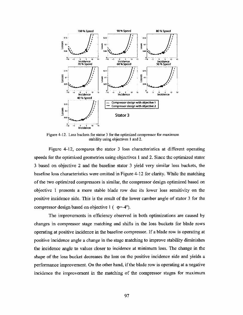
100 % Speed 90 % Speed 80 % Speed
0.15 1 - 10.15 0.15
Incidence Incidence Incidence40 % Speed _______________
0.1s ...I Compressor design with objective 1S -Compressor deinwith objective 2
Stator 3
V1 0.1
00 -5 0.0 % 0
Incidence
Figure 4-12. Loss buckets for stator 3 for the optimized compressor for maximumstability using objectives 1 and 2.
Figure 4-12, compares the stator 3 loss characteristics at different operating
speeds for the optimized geometries using objectives 1 and 2. Since the optimized stator
3 based on objective 2 and the baseline stator 3 yield very similar loss buckets, the
baseline loss characteristics were omitted in Figure 4-12 for clarity. While the matching
of the two optimized compressors is similar, the compressor design optimized based on
objective 1 presents a more stable blade row due its lower loss sensitivity on the
positive incidence side. This is the result of the lower camber angle of stator 3 for the
compressor design based on objective 1 ( <p=-.4 *).
The improvements in efficiency observed in both optimizations are caused by
changes in compressor stage matching and shifts in the loss buckets for blade rows
operating at positive incidence in the baseline compressor. If a blade row is operating at
positive incidence angle a change in the stage matching to improve stability diminishes
the incidence angle to values closer to incidence at minimum loss. The change in the
shape of the loss bucket decreases the loss on the positive incidence side and yields a
performance improvement. On the other hand, if the blade row is operating at a negative
incidence the improvement in the matching of the compressor stages for maximum
97
stability and the stabilization of the blade rows further increase the losses and
deteriorate the efficiency of the compressor.
4.6 Summary
The compressor design optimization framework implemented for a 3 stage
compressor has been implemented for two different design philosophies. The first
philosophy consists in enhancing compressor efficiency at high speeds and the second
to improve the compressor dynamic stability throughout the operating envelope.
The compressor design optimization for maximum efficiency indicates that the
main mechanism behind the enhancement in compressor efficiency is to adjust the stage
matching in order to operate at incidence angle near minimum loss. If an individual
blade row is close to stall the optimizer reduces the operating incidence to values closer
to incidence at minimum loss. If on the other hand an individual blade row is close to
choke the opposite occurs. The changes in operating incidences are the result of
modifications to the inlet metal angle of the blade row considered and the outlet metal
angle of the preceding blade row. The results of the compressor design optimization for
enhanced efficiency are encouraging since an average increase in efficiency of 1% is
obtained across the operating envelope and a 2.7% enhancement of efficiency is
obtained at maximum climb condition. Further, the optimization for enhanced
efficiency also provides an improvement in stability with an average gain in surge
margin per NASA definition of 3 points throughout the working line.
The second design philosophy aimed at improving dynamic stability across the
compressor map. The results of the compressor design optimizations for maximum
stability indicate that there are two mechanisms to enhance compressor stability. The
first mechanism is governed by changes in stages matching to operate at lower
incidences. This is achieved by decreasing the inlet flow angle while keeping the inlet
metal angle constant. The second mechanism to enhance dynamic stability is related to
changes in the loss sensitivities which can be achieved through decreases in blade row
camber. The results of this second approach are also promising since dynamic stability
is shown to be improved by 23% and surge margin as defined in industry by 3.8 points
throughout the operating envelope.
98

The three compressor optimization case studies carried out in this thesis clearly
illustrate the impact of the different design philosophy on the compressor blade row
geometry since the three yield three different compressor architectures.
99
Chapter 5
Summary and Conclusions
This thesis introduces a new way to quantify the stability of compression
systems. Unlike surge margin, the new metric is directly related to the damping of the
natural oscillations of the compression system that lead to rotating stall and surge.
Furthermore, the new metric captures the shape of the compressor characteristic such
that it accounts for the sensitivity of compressor stability to changes in operating line
conditions. This metric is used as a primary design variable in a compressor
optimization design framework with the goal to enhance compressor performance and
operability. The novel design methodology is applied to a generic three repeating stage
axial compressor. The baseline three-stage compressor design is optimized to
demonstrate the potential performance and operability improvements. More
specifically, the work presented in this thesis addressed the following objectives:
5.1 Assessment of the Shortcomings of Surge Margin
Surge margin is the commonly used metric to quantify the stability of a
compression system. There are two definitions used in practice: the first definition
quantifies the margin in pressure ratio between surge point and operating point at
constant corrected mass flow whereas the second definition considers the change in
outlet corrected flow between the operating point and the surge point for the same
corrected rotational speed.
Both definitions are currently in use to guarantee that instabilities are avoided
throughout the compressor operating envelope. The rotating stall and surge instabilities
are the mature forms of the natural oscillations of small perturbations in the flow field,
and the damping of these oscillations is directly related to the slope of the compressor
100
characteristics. To contrast the surge margin metrics with the actual damping ratios of
the flow field oscillations, the stability of a three-stage compressor is quantified by the
two surge-margin definitions and by computing the changes in damping ratio along the
operating line. The results indicate that there is no correlation between the three stability
assessment methods and that the changes in damping ratio along the operating line
much more fundamentally represent the dynamic behavior and stability margin of the
compression system. Furthermore it is noted that, in comparison, surge margin is a more
conservative measure of stability and it is conjectured that a stability metric based on
dynamic considerations could potentially enable compressor designs with enhanced
performance.
5.2 Development of a New Stability Metric Based on
Dynamic Considerations
Based on the comparison between surge margin and the damping ratio of the
natural flow field oscillations a new stability metric is developed. The dynamic
compressor stability metric is comprised of two parts. In the first part, the dynamic
behavior of the compression system at operating conditions is captured by quantifying
the growth rate of the perturbations in the flow field. As predicted by the Moore-
Greitzer [19] theory this quantity depends on the slope of the non-dimensional total-to-
static pressure rise characteristic and thus is closely related to the compressor blade
rows loss characteristics. The second part of the new stability metric quantifies the
deterioration in the compressor dynamic stability with changes in working condition
and is referred to as robustness of dynamic stability to changes in operating conditions.
To illustrate the importance of this attribute of the new stability metric an example is
used where the relation between the shape of the non-dimensional pressure rise
characteristic and the robustness is demonstrated. In order to capture the entire shape of
the pressure rise characteristic, robustness is defined as the geometric mean of the local
curvatures of the pressure rise characteristic in the operating range of interest. The new
stability metric is then defined as a compound of both attributes. Weighting factors can
be assigned to each of the attributes in order to capture different operability
requirements. Next, the surge margin and the new stability metric are computed for a
101
three-stage baseline compressor to assess the benefits of the new metric. The results
show that the surge margin per the industry definition does not correlate with the new
metric and that surge margin as defined by NASA can qualitatively capture some of the
dynamic stability trends. However, only the new stability metric is able to quantify the
dynamic behavior of the compression system and is thus suggested to be used as a
prime design variable in the novel compressor design optimization framework.
5.3 Implementation of the New Stability Metric in a
Compressor Design Optimization Framework
A new compressor design optimization framework is implemented based on the
previous effort by Perrot [20]. The optimization allows a versatile definition of the
objective function such that any combination of pressure ratio, efficiency and dynamic
stability can be prescribed. Furthermore, the final objective function can include
individual objectives at various operating speeds. This is a key feature which allows to
achieve the best possible compromise between objective functions at design and off-
design operating conditions.
The compressor design optimization framework uses an effective blade-to-blade
CFD method (fast blade performance prediction method) to predict the blade row
performance which is used to evaluate the compressor performance and dynamic
stability. The fast blade performance prediction method consists of an N-dimensional
interpolation method in conjunction with a blade performance database that is generated
using MISES. The method enables to estimate the blade performance in dependence of
a number of user defined geometric blade parameters. The fast blade performance
prediction method is estimated to be 100 times faster than a direct numerical simulation
and it is shown that the accuracy is within 2% of the direct numerical simulation results.
5.4 Application of the Compressor Design Optimization
Framework to a Generic Three Stage Compressor
One of the key objectives of this research is to apply the novel compressor
design methodology to the three-stage baseline compressor. To assess the potential
102
benefits of adopting this methodology in the design phase, two different design
philosophies commonly used in compressor design practice were adopted.
The first design philosophy used in the optimization is aimed at improving
efficiency, especially at operating speeds where a low specific fuel consumption is
desired.
The second optimization design philosophy implemented in the compressor
design framework is targeted to improve operability over the entire compressor
operating range without variable stator geometry and inter-stage bleed valves as it is
often the case for low pressure compressors. Such a compressor design optimization
could potentially reduce the complexity of the compressor architecture and increase the
thrust-to-weight ratio.
5.5 Demonstration of Performance and Operability
Enhancements using the Novel Compressor Design
Methodology
To demonstrate the potential performance improvements using the compressor
design optimization framework the two design philosophies are implemented. The
major goal is to enhance the compressor efficiencies at high speed and to improve the
operability throughout the operating envelope.
The results of the compressor design optimization for enhanced efficiency
demonstrate that improvements in efficiency are due to an optimal matching of the
compressor stages. The optimum stage matching which entails incidence angles close to
minimum loss conditions is achieved through changes in the blade row inlet and exit
metal angles. The results of the compressor design optimization for maximum
efficiency are promising: an average efficiency improvement of 1% is obtained
throughout the operating envelope, and at maximum climb conditions an efficiency
enhancement of 2.7% is achieved. Furthermore, optimizing for efficiency does not
deteriorate stability but yields an average improvement in surge margin per the industry
definition of 2.6 points along the working line. In addition, the impact of the operating
line constraints on optimized compressor performance was assessed. It is demonstrated
103
that an additional 1% efficiency improvement can be obtained if the pressure ratio
variations along the operating line are allowed to vary by 4%.
The compressor design optimization based on enhanced dynamic stability
provides on average a 23% improvement in the newly developed stability metric which
translates into a surge margin enhancement of 4 points on average across the entire
compressor map. The dynamic stability enhancements are the result of improvements in
compressor stage matching and of modifications in the loss buckets due to geometric
changes in the blade profiles. An improvement in compressor matching for enhanced
dynamic stability demands incidence angle changes which can be achieved through
changes in the outlet metal angle of the preceding blade rows and by decreasing the
camber angle. Furthermore it is observed that the compressor design optimization for
enhanced dynamic stability also implies improvements in compressor efficiency
although the optimization objective does not explicitly account for efficiency
improvements. In particular, for the cases investigated, the compressor efficiency was
improved by an average of 0.65 points throughout the operating envelope.
5.6 Recommendations for Future Work
The research effort presented in this thesis constitutes the definition of a new
compressor stability metric and a proof-of-concept study of a novel compressor design
optimization method. To achieve these goals within the timeframe of this thesis many
assumptions had to be made. Based on these and the outcomes of this research, the
following recommendations can be made for future work.
The mean-line flow solver and the dynamic model assume two-dimensional
flow and thus neglect three-dimensional effects such as endwall losses and hub corner
stall. These three-dimensional loss effects are important in advanced compressor
designs and should be included in the optimization framework. Furthermore the fast
blade prediction method should be extended to predict blade deviation angles in order to
replace the empirical correlations currently used in the framework.
Alternative CFD flow solvers are envisaged in the fast blade performance
prediction method to enable the performance assessment of a broader range of blade
geometries and flow conditions: in particular very large stagger angles, camber angle
104

and higher Mach numbers (transonic conditions). Moreover, the blade performance
database can be readily extended to more than two geometric variables used in this
thesis. This would yield further degrees of freedom in the optimization process and
potentially enable even larger performance and operability enhancements.
In summary, the outcomes of this thesis are encouraging and it is suggested to
apply the developed optimization framework and novel stability metric to an industrial
strength problem to assess the capabilities in a real compressor environment.
105
Appendix A
Description of Blade Row Losses andDynamics
This appendix describes the approach adopted to evaluate the sensitivities of
blade row loss to changes in flow inlet conditions and presents the modifications to the
transmission matrices in the rotating stall inception prediction model. The ducts in the
model are considered inviscid and hence no changes to the transmission matrices of
these components are required (for information on the derivation of the transmission
matrices of ducts/gaps refer to Spakovszky [24]).
A.1 Losses
The sole sources of blade row losses included in the calculations throughout this
thesis are blade profile losses. These are calculated using blade-to-blade CFD (MISES
or blade performance prediction method) and are represented by the loss
coefficient w = ' . The dynamic compressor model requires a slightly differentPa - P 1
description of the blade row losses, namelyL = 2 and thus the resulting losspU2
coefficients obtained from CFD need to be modified before introducing them into the
dynamic compressor model. Assuming incompressible flow, the two definitions are
related according to:
L = Y
Due to the difficulty in experimentally of measuring flow angles the dependence
of loss coefficient with incidence is generally not available. Instead, the dependence of
106
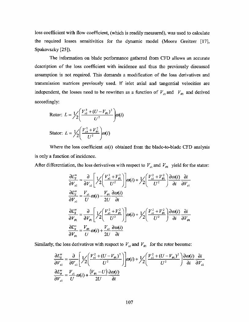
loss coefficient with flow coefficient, (which is readily measured), was used to calculate
the required losses sensitivities for the dynamic model (Moore Greitzer [17],
Spakovszky [25]).
The information on blade performance gathered from CFD allows an accurate
description of the loss coefficient with incidence and thus the previously discussed
assumption is not required. This demands a modification of the loss derivatives and
transmission matrices previously used. If inlet axial and tangential velocities are
independent, the losses need to be rewritten as a function of V', and V.1 and derived
accordingly:
V X +(U - V1)2Rotor: L = 1 (0U)
V1 +ViStator: L = 1 u2 }()
Where the loss coefficient a)(i) obtained from the blade-to-blade CFD analysis
is only a function of incidence.
After differentiation, the loss derivatives with respect to Vx, and Vo1 yield for the stator:
a F 1 (V+V V +V) a+V(i) Jiavs, a Y2 2 j~l + 2 u2 )l ajj aia VX a VX U2U ai a VXaLi V V, aw(i)
- = --- 9(i)aVs1 U 2U ai
L a F Vrv +VV+Vi a(V(i)a i
av',1 aVol 2 U2 U2a)Vol
aL _ V1 V a w(i)a)(i) +
aVol U 2U ai
Similarly, the loss derivatives with respect to Vxl and V.1 for the rotor become:
aLi a V+(U , V +(U -V 1 )2 a(i) ai
aVX, aV1 L 2 u2 Y2 U 2 ai a V,( U) a( 9)(i)
aV', U 2U ai
107
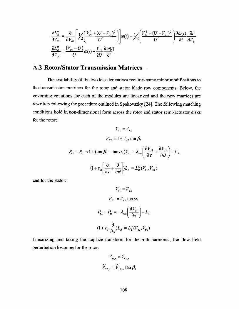
LR _ 1 V +(U- V 1 +(U -V 1) 2 a((i) ai
aVo1 aV1 2 u 2 Y2 u2 ai a V,1
aLR (V, - U) Vx1 aa(i)= (0(i)
aV,1 U 2U ai
A.2 Rotor/Stator Transmission Matrices
The availability of the two loss derivatives requires some minor modifications to
the transmission matrices for the rotor and stator blade row components. Below, the
governing equations for each of the modules are linearized and the new matrices are
rewritten following the procedure outlined in Spakovszky [24]. The following matching
conditions hold in non-dimensional form across the rotor and stator semi-actuator disks
for the rotor:
x1 x2
V 2 =1+ Vx2 tan 2
P2- =1+(tan _2 tana,)Vx, - a + - LR(I+ Zl xl + I) -LV o
r R R x1a]1Lal- aojand for the stator:
x1 x2
V0 2 = Vx 2 tan a 2
t2 - tl = -Asta ( ar )_L~saV
aTrLinearizing and taking the Laplace transform for the n-th harmonic, the flow field
perturbation becomes for the rotor:
Vxln = Vx2,n
V9 2 ,n = Y2,. tan/62
108
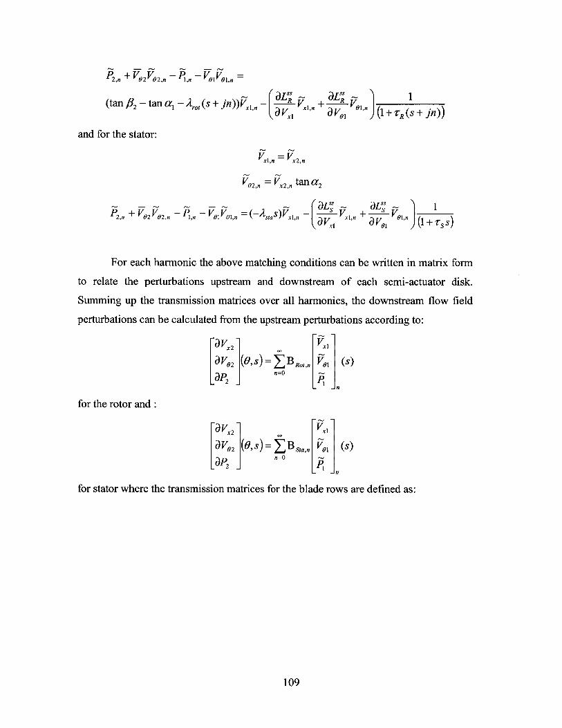
2,n + 2V02,n P1,n -VoiVOi,n =
~ (aLS ~ L"~ 1(tan$ 2 - tan ai - Aot(s + jn))Vxi- R V + R Vo1n_(tan A 'n -( a v V , n a V o , n ,, ( + R)
and for the stator:
x1,n x 2,n
IVi 2,n = x2,n tan a2
2,n + V 2 V2,n , 1 , sta xl,n av xl,n + 1 + ,nXs aVl (1+rss)
For each harmonic the above matching conditions can be written in matrix form
to relate the perturbations upstream and downstream of each semi-actuator disk.
Summing up the transmission matrices over all harmonics, the downstream flow field
perturbations can be calculated from the upstream perturbations according to:
aVx2 xI
aV02 ( = BRot,n (S)
a2 n 0
for the rotor and:
a Vx2 1Xa V02 (os) = EBstan[ V ] (s)
P2 sPt
for stator where the transmission matrices for the blade rows are defined as:
109
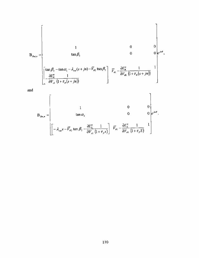
1
tanf 2
tan$P2 - tanal (S + in)- V.2 tan$ 2
aV. (1+rR
1
tan a 2
0
0
-~ aLSS
* a -Voi (1+TR(s + n))
0 0
0 0 le "
- AsaS - V02
3L"S 1 1tan fi2 rs s
- 3L's 1V " 3 Vg , IrsS
110
BRot,n =
10
0 jno
and
1
BSta,n =
1
Bibliography
[1] BLANVILLAIN, E., "Dynamic Stability Analysis of a Multi-Stage Axial
Compressor with Design Implications". Master's Thesis, Department of Aeronautics
and Astronautics, Massachusetts Institute of Technology, Feb. 2003.
[2] BONNAURE, L.P.,"Modelling High Speed Multistage Compressor
Stability". Master's thesis, Massachusetts Institute of Technology, 1991.
[3] BUCHE, D., GUIDATI, G., STOLL, P.,"Automated Design Optimization of
Compressor Blades for Stationary, Large-Scale Turbomachinery". GT2003-38421.
Proceedings of the ASMA Turbo Expo 2003.
[4] CAMP,T.R., DAY, I.J.,"A Study of Spike and Modal Stall Phenomena in a
Low-Speed Axial Compressor". Journal of Turbomachinery, Transactions of the ASME,
Vol. 120 (1998), pp. 393-401.
[5] CUMPSTY, N., "Compressor Aerodynamics". Addison-Wesley Publishing
Company, 1998.
[6] DAY, I.J., "Stall Inception in Axial Compressors". Trans. ASME Journal of
Turbomachinery, VOL. 155, pp. 1-9.
[7] DORCA, J.M.,"Aplication of an Energy-Like Stability Metric for Axial
Compressor Design", Master's Thesis, Department of Aeronautics and Astronautics,
Massachusetts Institute of Technology, 2003.
[8] FEULNER, M.R., "Modeling and Control of Rotating Stall in High Speed
Multi-Stage Axial Compressors". Ph.D. thesis, Massachusetts Institute of Technology,
1994.
[9] FRECHETTE, L.G., "Implications of Stability Modeling for High-Speed
Axial Compressor Design". Master's Thesis, Department of Aeronautics and
Astronautics, Massachusetts Institute of Technology, Feb. 1997.
[10] GARZON, VICTOR E.; DARMOFAL, DAVID L., "Impact of geometric
variability on axial compressor performance". American Society of Mechanical
111
Engineers, International Gas Turbine Institute, Turbo Expo (Publication) IGTI, v 6 B,
2003, p 1199-1213
[11] GREITZER, E.M., WISLER, D.C.," Gas Turbine Compressor Technology:
Status and opportunities", IGTIC 1999.
[ 12] GREITZER, E.M., "Review - Axial Compressor Stall Phenomena", Journal
of Fluids Engineering (Jun. 1980), Vol. 102, pp. 134-168.
[13] GREITZER, E.M., "Stability of Pumping Systems - The 1980 Freeman
Scholar Lecture", Journal of Fluids Engineering (Jun. 1981), Vol. 163, pp. 193-240.
[14] KERREBROCK, J.L., "Aircraft Engines and Gas Turbines", 2"d ed. The
MIT Press, Cambridge, Massachusetts, 1992.
[15] LAMB, CAROLINE TWOMEY; DARMOFAL, DAVID L.,
"Performance-based geometric tolerancing of compressor blades". Proceedings of the
ASME Turbo Expo 2004, v 5 A, 2004, p 203-210.
[16] LIEBLEIN, S., SCHWENK, F.C., BRODERICK, R.L., "Diffusion Factor
for Estimating Losses and Limiting Blade Loadings in Axial Flow Compressor Blade
Elements". NACA RM E53D01, 1953.
[17] LONGLEY, J., "A Review of Nonsteady Flow Models for Compressor
Stability", ASME J. of Turbomachinery (Apr. 1994), pp. 202-215.
[18] MCDOUGALL, N.M., CUMPSTY, N.A., HYNES, T.P., "Stall inception
in axial compressors ". Journal of Turbomachinery, VOL. 112 (1990), pp. 116-125.
[19] MOORE, F., AND GREITZER, E., "A Theory of Post-Stall Transients in
Axial Compressors: Part I - Development of the Equations", ASME J. of Engineering
for Gas Turbines and Power, Vol.108 (1986), pp. 68-76.
[20] PADUANO, JAMES D., E.M. GREITZER, A.H. EPSTEIN, "Compression
System Stability", Annual Rev. Fluid Mechs, 2001, 33:491-517.
[21] PERROT, V., "A Design Optimization Framework for Enhanced
Compressor Stability Using Dynamic System Modeling", Master's Thesis, Department
of Aeronautics and Astronautics, Massachusetts Institute of Technology, Aug. 2003.
[22] SIDWELL, VINCE; DARMOFAL, DAVID, "A selective assembly method
to reduce the impact of blade flow variability on turbine h'fe
Source ", Proceedings of the ASME Turbo Expo 2004, v 5 A, 2004, p 267-276.
112
[23] SIEVERDING, F., CASEY, M., RIBI, B., MEYER, M., "Design of
Industrial Axial Compressor Blade Sections for Optimal Range and Performance".
GT2003-38036. In Proceedings of the ASME Turbo Expo 2003.
[24] SMITH, L.H., "Compressor Aero Design at General Electric Before CFD".
Journal of Turbomachinery, Vol.124 (2002), pp. 321-330.
[25] SPAKOVSZKY, Z., "Applications of Axial and Radial Compressor
Dynamic System Modeling", PhD Thesis, Department of Aeronautics and Astronautics,
Massachusetts Institute of Technology, 2000.
[26] WECK, 0., WILLCOX, K., "Multidisciplinary System Design
Optimization", Class Notes, 16.888, MIT, Spring 2004.
[27] WEIGL, H.J., FRECHETTE, L.G., "An Update on Compressible Stall
Inception Modeling". MIT Gas Turbine, Internal Document, 1997.
[28] YOUNGREN, H., DRELA, M., "A User Guide to Mises 2.53". MIT,
Computational Aerospace Sciences Laboratory, December 1998.
113