Online Submission ID: 0

A Novel Distance Measure for Ocean Reconstruction from SparseObservations Demonstrated on the Atlantic

Category: Research

ABSTRACT

We introduce a distance measure for use in scattered data approx-imation. Reconstruction from sparse, non-uniformly distributeddata should utilize application-specific knowledge to produce high-quality results. Our distance measure is considering the specificproblem of computing reconstructions from sparse observationalpaleoceanography data, where it is possible to consider certainproblem-specific knowledge to produce reconstructions of scien-tific value. Our approach to the problem combines the new distancemeasure with the well-known moving least squares (MLS) method.We demonstrate that our approach produces high-quality results, bycontrasting our distance measure against Euclidean and geodesicdistances. We have used our method to generate reconstructionsfrom data in the Atlantic Ocean.

1 INTRODUCTION

One of the fundamental challenges in the study of climate changethroughout Earth’s history is how to combine models of past oceancirculation, as reconstructed from sparse geochemical data col-lected from deep sea sedimentary cores, with modern ocean circu-lation data to yield insight into the processes governing ocean circu-lation in the past. We approach this challenge through the analysisof carbon isotope datasets that have been generated from analysesof microfossils collected from deep sea cores [12].

Previous synthesis studies of circulation changes during the LastGlacial Maximum (LGM, 20,000 years before present time) fo-cused on geochemical data from benthic foraminifera in only twodimensions, water depth and latitude (e.g., [3]). Compiled and syn-thesized data in the third (longitude) and fourth (time) dimensionswould provide important constraints on overturning rates and watermass boundary variations along flow paths that are not yet available.

Continuous records of foraminifera data are mainly found atocean depths less than 4.5km, which corresponds to the continen-tal margins along the ocean basin periphery, elevated topographicareas and the mid ocean ridges. With carbon isotope records from∼480 deep sea cores [12], combining these data to produce a three-dimensional perspective of ocean current distribution through timerequires an interpolation methodology that links data across thou-sands of kilometers in the latitude/longitude domain, and hundredsof meters across the vertical water column.

The characteristics of the data (few data points, sparse and non-uniform distribution, differences in length ratios, data points avail-able only at the border of the interpolation space) are challengingfor commonly used interpolation schemes, therefore providing themotivation for the research described in this paper. To address thepressing need for specialized schemes handling such a challengingdata set, we designed a method that combines a reliable interpo-lation scheme with a novel distance measure. This distance mea-sure is learned via training performed on the data itself in a pre-processing step. The most important advantages of the method arethat it does not need additional information (e.g., a flow field) andhas self-optimizing parameters (e.g., compensating differences inlength ratios).

2 RELATED WORK

Scattered Data Interpolation: Franke et al. [6] provided anoverview of existing interpolation methods and evaluates them on

some examples for the reconstruction of surfaces. They noted thatthere existed real data sets with characteristics similar to those wehave (sparse and scattered) for which some of the considered meth-ods perform poorly. Unfortunately they have not further investigatethis aspect.

A well-known interpolation scheme for irregularly distributeddata is MLS, which was introduced by Levin in [10]. This methodproduces high-quality results for the approximation of shapes, evenwhen the data is noisy. A comparison of different approaches ofMLS is given in [2]. The main reasons that we have chosen thismethod to demonstrate our novel distance measure are its robustbehavior against noise, its flexibility and that it is proven to be use-ful in a wide range of applications.

Interpolation in the field of Oceanography Due to the un-certainty in ocean observations, oceanographers recognized earlythat linear interpolation methods, such as Aitken-Lagrange inter-polation [4], were unsatisfactory as they were fitting observationalnoise. In increasing order of complexity, oceanographers have im-plemented nudging techniques (e.g., [11]), temporally sequentialrecursive least-squares methods (i.e., Kalman filter [5]), and whole-domain least-squares methods (i.e., four-dimensional variationaldata assimilation, Stammer et al. [16]). The primary drawbackwith the later methods is the computational expense of represent-ing oceanic fields and the uncertainties.

More recently, least-squares methods have permitted the recon-struction of global, four-dimensional (i.e., time-varying and spatial,globally) property fields over the last 30,000 years [7] and the LastGlacial Maximum [8]. Such methods have succeeded in reproduc-ing the observations within their uncertainty, obey ocean dynamicsand boundary conditions including bathymetry, and simultaneouslyreproduce multiple property fields, but require large memory andcomputational resources.

3 METHOD DESCRIPTION

In order to present our novel distance measure we have chosen MLSas underlying fundamental reconstruction scheme. We first brieflyoutline this method, for the sake of completeness and then give adetailed description of the proposed distance measure.

3.1 Moving Least SquaresMLS is a commonly used method for the approximation of scat-tered data in computer graphics [10]. Since it is a well-known tech-nique and not the focus of this work we provide only a short intro-duction of what we need for the description of our distance measureand the demonstrations in Section 4.

For the purposes of this work we use the general matrix form ofMLS given by Shen in [14] to find a function f that approximatesthe values F of a set of unorganized sample points:

f (x) = bT (x)(BT (W (x))2B)−1BT (W (x))2F (1)

The matrix B contains a number of basis functions b. For exam-ple, a linear basis for a three dimensional problem has the functions1, x, y, and z. W is a diagonal weight matrix depending on weighteddistances, which we calculate using the inverse distance function asgiven in [14]:

w(d) = 1/(d2 +λ2), (2)

1

Online Submission ID: 0

where λ is a parameter to control the approximation behavior andd is a distance between two points. Obviously the distance measurehas a significant influence on the weights and thereby the recon-struction.

3.2 Proposed Distance MeasureA new data-driven distance measure for two points P1 and P2, givenin spherical coordinates, is presented. It is used in our proposed ap-proach, but could also be integrated in another interpolation schemethat must calculate distances between sample points of spherical na-ture.

x

y

z

(r,θ,Φ)

rΦ

θ

(a)

P1

P2

Δ (θ)

Δ (Φ)

Δ (r)

(b)

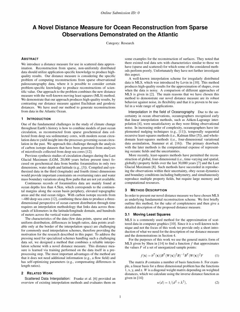
Figure 1: (a) In the spherical coordinate system the position of apoint is described by three variables r, θ and φ . (b) Our proposeddistance measure is a weighted combination of differences of thosecomponents (∆(θ), ∆(φ) and ∆(r)).

In spherical coordinates, a point is described by a radius r andtwo angles θ , φ as shown in Figure 1a. If two points P1 =(r1,θ1,φ1) and P2 = (r2,θ2,φ2) are located on the surface of thesame sphere, which means that r1 is equal to r2, the shortest pathbetween them is part of a great circle. The geodesic distance canfor example be computed by the Haversine formula [15]:

dgeodesic(P1,P2) = 2r1atan2(√

Q,√

1−Q) (3)

where

Q = sin2 ((φ2−φ1)/2)+ cos(φ1)cos(φ2)sin2 ((θ2−θ1)/2) .

Equation 3 is correct as long as the points lie on the same sphere.If r1 and r2 differ one could for example compute the resulting dis-tance as follows:

davgGeodesic(P1,P2) =dgeodesic(P1,P122)+dgeodesic(P211,P2)

2(4)

whereP122 = (r1,φ2,θ2) and P211 = (r2,φ1,θ1).

In applications like oceanography it is not always clear what a dis-tance between two points should be. This is due to the fact that wa-ter cannot flow from one position to another by following a straightline or a great circle when this is not implied by the flow field. Tothis end, a high-quality distance measure would be one that consid-ers the flow as proposed by Streletz et al. [17]. Our method assumesthat flow information is not given, and we therefore must restrict ourdistance measure purely on the data available.

In the absence of flow field information, we therefore consider aweighted combination of differences in the three spherical coordi-nates r, θ , and φ (see Fig. 1b). Our distance between two points P1and P2 is defined by Equation 5. We consider the following genericpoints P112 = (r1,φ1,θ2), P211 = (r2,φ1,θ1), P212 = (r2,φ1,θ2)and P122 = (r1,φ2,θ2). Our new distance measure is defined as:

dproposed(P1,P2) = α∆(φ)+β∆(θ)+ γ∆(r) (5)

where

∆(φ) = (davgGeodesic(P2,P212)+davgGeodesic(P122,P112))/2,

∆(θ) = (davgGeodesic(P1,P112)+davgGeodesic(P211,P212))/2,

∆(r) = |r1− r2|.

A machine-learning pre-processing step is performed to estimateadequate values for the weights α , β and γ , which is similar to aleave-p-out cross-validation. Specifically, this step proceeds as fol-lows: We repeatedly partition the input point set S randomly in twosubsets, a training set T and a validation set V . In every iteration iwe train αi, βi and γi on T , so that the resulting reconstruction usingMLS has a small root mean square (RMS) error for V . We termi-nate the process of parameter optimization when n iterations havebeen carried out. At this point, we assume that the values of thethree weights are properly adjusted for the data we are concernedwith.

Our optimization procedure has three input parameters: the set Sof data points, an integer p that is used to partition S and an integern that specifies the number of iterations. Additionally a matrix ABGis initialized to store the weights αi, βi, γi of the individual iterationi. The process is performed n times. In each iteration the followingsteps are executed. S is randomly partitioned in a training set T anda validation set V so that V has p elements. In our experiments agood choice for p was |S|/3. When p is chosen too small it results inoscillating weights of the individual iterations and the method doesnot converge. After initializing the weights αi, βi and γi with 1 theyare optimized on T to minimize the RMS error for V , using MLSas our approximation method of choice.

The simultaneous optimization of the weight parameters leads toa multidimensional optimization problem and is in general hard tosolve. Although more sophisticated approaches could be used, inour case it suffices to optimize αi, βi and γi sequentially. This isdone by repeating the following steps for several times: The valuesof each parameter are decreased or increased and overwritten by thevalue that produces the smallest RMS error for the current valida-tion set. This simple procedure suffices to demonstrate the viabilityof our approach, but it should be improved further. At the end ofevery iteration the optimized values are added to ABG.

Finally, the medians of the weights considering all iterations thatare stored in AGB are determined. This extracts the weights thathave produced the smallest errors in the most iterations and there-for are seen as meaningful for S. In contrast parameters leading tothe smallest errors in one iteration are often only optimal for thecurrent training set T . Using the median reduces the influences ofthe random configurations.

4 RESULTS

In the following, the performance of our distance measure in com-bination with MLS is demonstrated for two examples.

4.1 Analytically Defined DataFor our first demonstration we consider a volume element E of athin spherical shell defined by 6,360km≤ r ≤ 6,371km, 0◦ ≤ θ ≤45◦ and 0◦≤ φ ≤ 45◦. 6,371km is approximately the Earth’s radius,and the thickness of this shell approximates the depth of the Mari-ana Trench, which is the lowest location of the ocean. In summary,we consider the four layers in this volume:

g(r,θ ,φ) =

1 r < 6,363km2 6,363km≤ r < 6,364km4 6,364km≤ r < 6,367km5 r ≥ 6,367km

(6)

2

Online Submission ID: 0

We consider the function g in E and distribute randomly pointswithin this volume. Our goal is to reconstruct all reference pointson a 0.5km×1◦×1◦ grid from these sparse data. We call the set ofour input points test data set and the set of points that should be re-constructed, and for which the exact values are available, referencedata set. We compute the RMS error over all grid points exceptthose lying on the border of E.

The reconstruction itself is computed by using MLS with λ =0.0001 in the weight function, see Equation 2, and 1, x, y and zas the four basis functions. One step of MLS computes distances,which can be done in different ways. We compare the Euclidean,geodesic and our proposed distance measure for computing theneeded distance values. Only for our approach a pre-processingstep is performed once for every test data set. As described in Sec-tion 3 it uses three input parameters. In this case S is the set of therandomly distributed points. The second parameter p divides S intwo subsets. An empirically confirmed choice for p is |S|/3, whichhas produced high-quality results in our experiments. The last pa-rameter n defines the number of iterations to perform the trainingfor weights. We set n to 100 for this experiment, which is sufficientconsidering the small amount of data points. In Section 4.2.2 weinvestigate how this parameter has to be chosen for a real data set.

Our experiment is divided in two parts. The first part investigatesthe behavior of the reconstruction with decreasing number of sam-ple points and the second part analyzes the robustness of the resultswhen changing the distribution of a fixed number of points.

For the first part we randomly pick 30 points in E and gener-ate progressively smaller subsets with 30, 25, 20, 15 and 10 datapoints. MLS together with all three distance measures is used toreconstruct the reference test data set, and the resulting RMS errorsare computed. For this test data set our proposed distance measureproduces the smallest RMS errors (< 0.3377) in all cases. This isdue to the specialization of our method for such problems (sparsedata, differences in length ratios, functions with a layer character-istic). The RMS errors (> 1.9376) produced by using Euclideanand geodesic distance are close to each other and relatively stable,but about one order of magnitude larger than the RMS error valuesobtained with our distance measure.

The question remains whether the results produced with the pro-posed distance measure are relatively invariant under a change ofpoint distribution. To examine this aspect we generated 50 test datasets with 10 randomly distributed points in each case and computedthe resulting RMS errors. It is remarkable that our proposed ap-proach works well in this scenario. Even for extreme distributionsit is consistently better when compared to the results computed withthe other two distance measures. Only the variability of the result-ing errors is larger than in the case of Euclidean and geodesic dis-tance.

4.2 Atlantic Ocean DataAs shown in the previous section our proposed approach works wellfor a analytically defined data set. However, the actual goal is toreconstruct the LGM δ 13C sediment core data set presented in Sec-tion 1. This task is more challenging due to large gaps in the dataas well as clusters resulting from data collection.

Since the actual LGM data set does not provide us with a groundtruth against which the reconstruction results can be evaluated, wecannot use it directly to perform a proof of concept. For this reason,we construct a data set of the modern ocean based on the locationsgiven by the LGM data set. Further, we limit the data set to theAtlantic Ocean, because it is the best-observed ocean basin duringglacial times.

4.2.1 Data Preparation

As reference data set, we use a subset of the World Ocean Cir-culation Experiment (WOCE) oceanography data [9] that was re-

leased with uncertainty estimates. WOCE organized, collected, andcompiled global ocean observations for the decade from 1988 un-til 1998. We consider the part between 53◦S to 60◦N latitude and98◦W to 18◦E longitude as representing the Atlantic Ocean. Thissubset contains points of the Pacific Ocean as well as MediterraneanSea, which we do not need for the reconstruction of the Atlantic andfor that reason we removed them. Since we only have data locatedat the sea floor it would be improper to consider the part between0m and 1,000m depth, due to the extremely strong mixing in thisinterval and the interaction with the atmosphere. To this end, wedo not include this part in our experiment. Furthermore, we had touse phosphate as substitute tracer instead of δ 13C, due to lack of agridded climatology of modern-day δ 13C. Using phosphate makessense, because it has nearly a linear relation to δ 13C [1]. Our re-sulting reference data set includes 419,623 grid points.

For our test data set we selected all nearest neighbors of the datapoints included in the LGM data set within our reference data set,resulting in 186 data points. The number of points is smaller thanthe actual number of core samples, because several points of theLGM data set are mapped to the same neighbors, as well as gaps inthe reference data set. This new subset has characteristics similarto the original LGM data set. We use our proposed approach togenerate a reconstruction based on these 186 representative corelocations of the modern ocean and compare it against the WOCEreference data set, which we assume as ground truth.

4.2.2 Proposed Approach

A pre-processing step is performed to obtain appropriate values forthe weights that are tuned to the actual data set. As described inSection 3 three input parameters are considered for this purpose.The first parameter S is our test data set that we have described inSection 4.2.1 with an amount of 186 data points. For the secondparameter p that defines the division of S we already obtained goodresults with |S|/3 in our prior example and for this reason choose it as186/3 = 62. The last parameter n, the number of trainings iteration,depends on the complexity of the function that is covered by S.Since this is difficult to capture, we use the following procedure.

We performed our optimization with a relative high value forn. For all three weight parameters after at least 200 iterations aconvergence of the values was recognizable. Therefore, we set n to200 for this experiment. Note that in the actual experiment we donot train the weights again using n = 200. Should new data pointsbe added to the test data set, this value can be used as a reference.The optimized values for the test data set are α = 0.015, β = 0.011and γ = 35.57. This clearly shows that the weights are specializedfor our problem. The length ratio in the ocean between differencesin depth and differences in latitude and longitude, respectively, arevery high. Our distance measure compensates for this effect bystretching in depth (= γ) direction.

Knowing our specialized, problem-specific weights, we use themtogether with MLS to reconstruct the reference data set. In thisexperiment we have chosen λ = 14 for the weight function (seeEquation 2), and as basis functions we have used the functions 1, x,y, z and yy.

4.2.3 Discussion

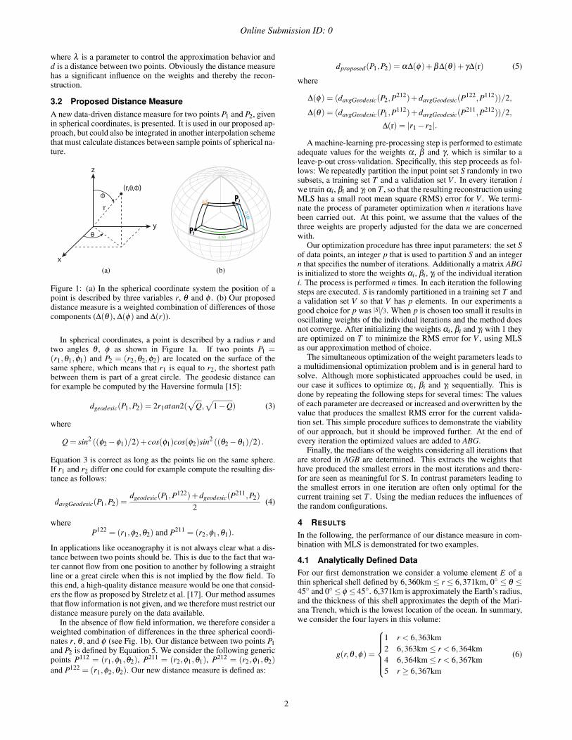
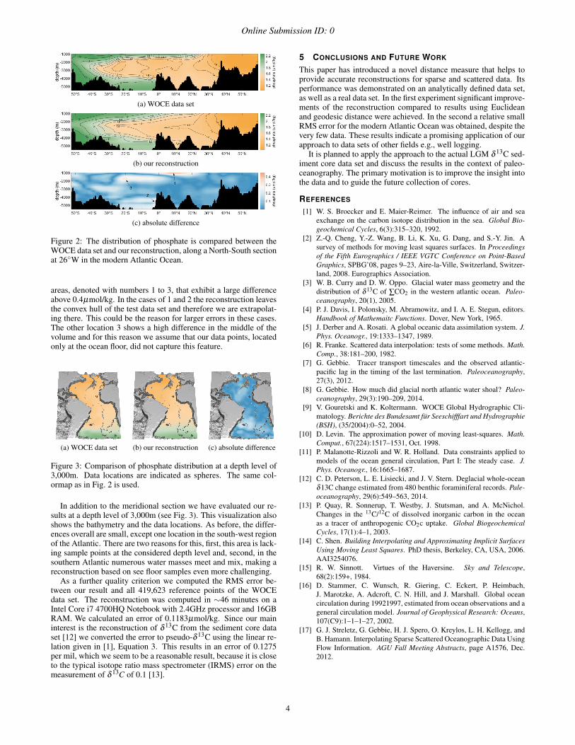
In order to investigate the performance of our reconstruction againstthe reference data set we do an visual comparison using sectionplots that cover significant parts of the reconstruction. For the At-lantic Ocean a popular visualization in literature is a North-South(meridional) section. For this reason we have generated compa-rable plots for our reconstruction as well as for the reference dataset by cutting out a section at 26◦W and from 40◦S to 60◦N (seeFig. 2). To highlight the largest deviations also the absolute dif-ference is given in Fig. 2c. The major part of this plot presents arelatively small difference below 0.1µmol/kg. There are only three

3

Online Submission ID: 0

(a) WOCE data set

(b) our reconstruction

(c) absolute difference

Figure 2: The distribution of phosphate is compared between theWOCE data set and our reconstruction, along a North-South sectionat 26◦W in the modern Atlantic Ocean.

areas, denoted with numbers 1 to 3, that exhibit a large differenceabove 0.4µmol/kg. In the cases of 1 and 2 the reconstruction leavesthe convex hull of the test data set and therefore we are extrapolat-ing there. This could be the reason for larger errors in these cases.The other location 3 shows a high difference in the middle of thevolume and for this reason we assume that our data points, locatedonly at the ocean floor, did not capture this feature.

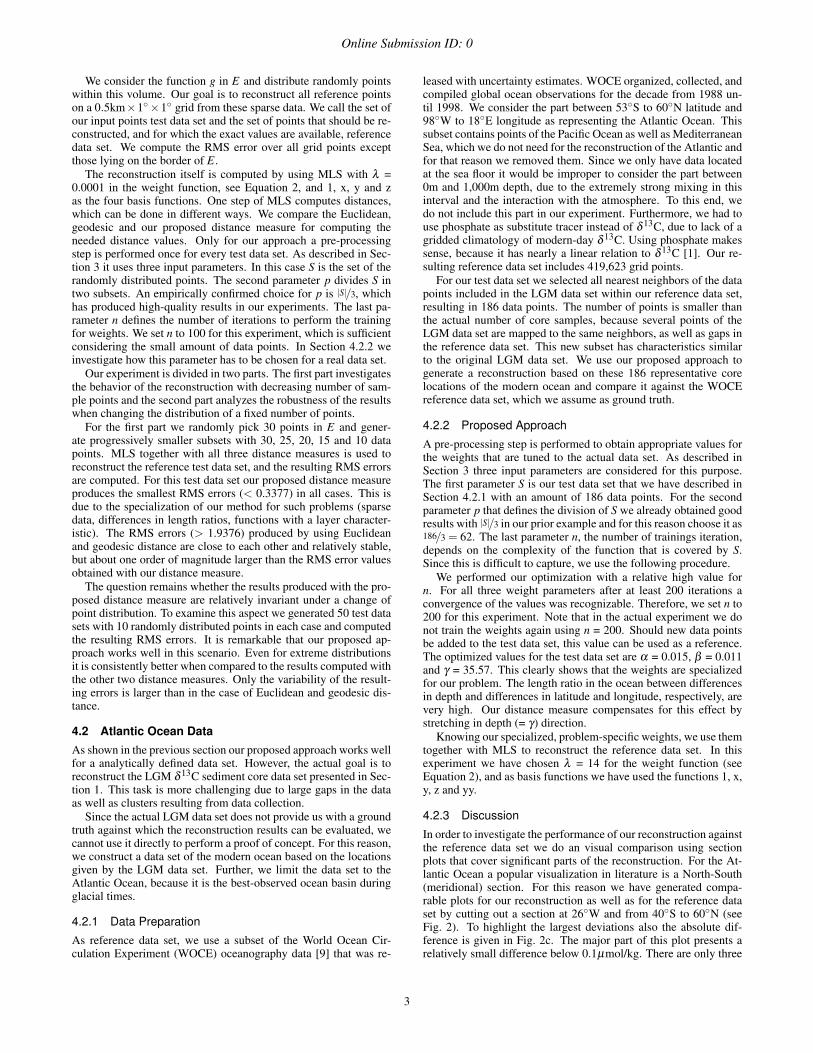
(a) WOCE data set (b) our reconstruction (c) absolute difference

Figure 3: Comparison of phosphate distribution at a depth level of3,000m. Data locations are indicated as spheres. The same col-ormap as in Fig. 2 is used.

In addition to the meridional section we have evaluated our re-sults at a depth level of 3,000m (see Fig. 3). This visualization alsoshows the bathymetry and the data locations. As before, the differ-ences overall are small, except one location in the south-west regionof the Atlantic. There are two reasons for this, first, this area is lack-ing sample points at the considered depth level and, second, in thesouthern Atlantic numerous water masses meet and mix, making areconstruction based on see floor samples even more challenging.

As a further quality criterion we computed the RMS error be-tween our result and all 419,623 reference points of the WOCEdata set. The reconstruction was computed in ∼46 minutes on aIntel Core i7 4700HQ Notebook with 2.4GHz processor and 16GBRAM. We calculated an error of 0.1183µmol/kg. Since our maininterest is the reconstruction of δ 13C from the sediment core dataset [12] we converted the error to pseudo-δ 13C using the linear re-lation given in [1], Equation 3. This results in an error of 0.1275per mil, which we seem to be a reasonable result, because it is closeto the typical isotope ratio mass spectrometer (IRMS) error on themeasurement of δ 13C of 0.1 [13].

5 CONCLUSIONS AND FUTURE WORK

This paper has introduced a novel distance measure that helps toprovide accurate reconstructions for sparse and scattered data. Itsperformance was demonstrated on an analytically defined data set,as well as a real data set. In the first experiment significant improve-ments of the reconstruction compared to results using Euclideanand geodesic distance were achieved. In the second a relative smallRMS error for the modern Atlantic Ocean was obtained, despite thevery few data. These results indicate a promising application of ourapproach to data sets of other fields e.g., well logging.

It is planned to apply the approach to the actual LGM δ 13C sed-iment core data set and discuss the results in the context of paleo-ceanography. The primary motivation is to improve the insight intothe data and to guide the future collection of cores.

REFERENCES

[1] W. S. Broecker and E. Maier-Reimer. The influence of air and seaexchange on the carbon isotope distribution in the sea. Global Bio-geochemical Cycles, 6(3):315–320, 1992.

[2] Z.-Q. Cheng, Y.-Z. Wang, B. Li, K. Xu, G. Dang, and S.-Y. Jin. Asurvey of methods for moving least squares surfaces. In Proceedingsof the Fifth Eurographics / IEEE VGTC Conference on Point-BasedGraphics, SPBG’08, pages 9–23, Aire-la-Ville, Switzerland, Switzer-land, 2008. Eurographics Association.

[3] W. B. Curry and D. W. Oppo. Glacial water mass geometry and thedistribution of δ 13C of ∑CO2 in the western atlantic ocean. Paleo-ceanography, 20(1), 2005.

[4] P. J. Davis, I. Polonsky, M. Abramowitz, and I. A. E. Stegun, editors.Handbook of Mathemaitc Functions. Dover, New York, 1965.

[5] J. Derber and A. Rosati. A global oceanic data assimilation system. J.Phys. Oceanogr., 19:1333–1347, 1989.

[6] R. Franke. Scattered data interpolation: tests of some methods. Math.Comp., 38:181–200, 1982.

[7] G. Gebbie. Tracer transport timescales and the observed atlantic-pacific lag in the timing of the last termination. Paleoceanography,27(3), 2012.

[8] G. Gebbie. How much did glacial north atlantic water shoal? Paleo-ceanography, 29(3):190–209, 2014.

[9] V. Gouretski and K. Koltermann. WOCE Global Hydrographic Cli-matology. Berichte des Bundesamt fur Seeschifffart und Hydrographie(BSH), (35/2004):0–52, 2004.

[10] D. Levin. The approximation power of moving least-squares. Math.Comput., 67(224):1517–1531, Oct. 1998.

[11] P. Malanotte-Rizzoli and W. R. Holland. Data constraints applied tomodels of the ocean general circulation, Part I: The steady case. J.Phys. Oceanogr., 16:1665–1687.

[12] C. D. Peterson, L. E. Lisiecki, and J. V. Stern. Deglacial whole-oceanδ13C change estimated from 480 benthic foraminiferal records. Pale-oceanography, 29(6):549–563, 2014.

[13] P. Quay, R. Sonnerup, T. Westby, J. Stutsman, and A. McNichol.Changes in the 13C/12C of dissolved inorganic carbon in the oceanas a tracer of anthropogenic CO2c uptake. Global BiogeochemicalCycles, 17(1):4–1, 2003.

[14] C. Shen. Building Interpolating and Approximating Implicit SurfacesUsing Moving Least Squares. PhD thesis, Berkeley, CA, USA, 2006.AAI3254076.

[15] R. W. Sinnott. Virtues of the Haversine. Sky and Telescope,68(2):159+, 1984.

[16] D. Stammer, C. Wunsch, R. Giering, C. Eckert, P. Heimbach,J. Marotzke, A. Adcroft, C. N. Hill, and J. Marshall. Global oceancirculation during 19921997, estimated from ocean observations and ageneral circulation model. Journal of Geophysical Research: Oceans,107(C9):1–1–1–27, 2002.

[17] G. J. Streletz, G. Gebbie, H. J. Spero, O. Kreylos, L. H. Kellogg, andB. Hamann. Interpolating Sparse Scattered Oceanographic Data UsingFlow Information. AGU Fall Meeting Abstracts, page A1576, Dec.2012.

4