Experimental Mechanics (2018) 58:183–206DOI 10.1007/s11340-017-0329-4

A Novel Image-based Ultrasonic Test to Map MaterialMechanical Properties at High Strain-rates

R. Seghir1 · F. Pierron1

Received: 9 February 2017 / Accepted: 14 August 2017 / Published online: 15 September 2017© The Author(s) 2017. This article is an open access publication

Abstract An innovative identification strategy based onhigh power ultrasonic loading together with both infraredthermography and ultra-high speed imaging is presented inthis article. It was shown to be able to characterize the visco-elastic behaviour of a polymer specimen (PMMA) froma single sample over a range of temperatures and strain-rates. The paper focuses on moderate strain-rates, i.e. from10 to 200 s−1, and temperatures ranging from room tothe material glass transition temperature, i.e. 110 ◦C. Themain originality lies in the fact that contrary to conven-tional Dynamic Mechanical Thermal Analysis (DMTA), nofrequency or temperature sweep is required since the exper-iment is designed to simultaneously produce both a hetero-geneous strain-rate state and a heterogeneous temperaturestate allowing a local and multi-parametric identification.This article is seminal in nature and the test presented herehas good potential to tackle a range of other types of highstrain-rate testing situations.

Keywords Ultra-high speed · Visco-elasticity · PMMA ·Infrared thermography · Identification

� R. Seghirr.seghir@soton.ac.uk

F. Pierronf.pierron@soton.ac.uk

1 Faculty of Engineering and the Environment,University of Southampton, Southampton, UK

Introduction

In many instances in life, materials around or within ussuffer deformation at high rates. This is the case when engi-neering structures undergo impact, crash, blast, etc. but alsowhen forming materials like stamping or machining forinstance. Another important area concerns biological tis-sues. For instance, traumatic brain injuries (TBI) involvedamage of brain tissues caused by their high rate defor-mation following impact load of the skull. Thanks to thesignificant progress in computing power and computationalmechanics tools, it is now possible to perform extremelydetailed numerical simulations of many complex situationswhere materials deform at high rates, with the objective todesign safer structures, assess tissue injuries or devise moreeffective manufacturing processes, as mentioned above.However, to deliver their full potential, these computationsrequire the input of reliable and accurate mechanical constitu-tive models of the materials loaded at high strain-rates. Thisis an extremely challenging problem because of both thedynamic nature of the mechanical fields and the technolog-ical difficulties associated with strain metrology. Presently,this represents an important scientific bottleneck for societyto fully benefit from such advances in numerical simulation.

A number of testing techniques are available to iden-tify the high strain-rate properties of materials, as reviewedin [5]. Most of them rely on very limited experimentalinformation, such as strain gauges or point velocity mea-surements with VISAR technology. As a consequence, thetests need to follow strict assumptions to relate the measure-ments to the material behaviour, for instance, uniform strainfield and no inertia effects are typical assumptions in splitHopkinson pressure bar (SHPB) testing.

184 Exp Mech (2018) 58:183–206

The advent of full-field optical metrology, such as digitalimage correlation [35] or the grid method [10], combinedwith the new developments in ultra-high speed imaging[2, 29, 36] provides a unique opportunity to revisit highstrain-rate testing techniques. In particular, full-field ofaccelerations can be obtained which provides a powerfulimage-embedded load cell if the material density is known,which is usually the case. This concept was first proposed in2009 in [22], published in full in 2011 [23], where a proofof principle experiment was performed on quasi-isotropiccomposite specimens, with and without a free hole. Thein-plane Young’s modulus and Poisson’s ratio were iden-tified satisfactorily before the onset of damage, within thefirst 30 μs of the test, at strain-rates up to 1000 s−1. Thegrid method was used to measure the deformation togetherwith a Cordin 550-62 rotating mirror ultra-high speed cam-era operating at 30 kfps. However, this test was performedon a tensile Kolsky bar, though the bars were not used toobtain the impact force. The concept was then extended topurely inertial tests which showed to be much more suitedfor this kind of analysis. The very first example dealt withconcrete spalling tests [26], and was then extended to com-posites [27] and metals [3, 4, 19]. Since then, the idea hasspread and several groups worldwide are starting to use thetechnique [13, 14, 16, 17, 21, 40, 41].

Initially, this idea to use the full-field acceleration as aload cell with the Virtual Fields Method came from seminalwork by Prof. Michel Grediac [8, 9] using vibration tests. Inthis case, high speed imaging is not necessary and the accel-eration derives easily from the deflection using the harmonicassumption. This was extended later on to include damping[7]. Recently, an article showed that ultrasonic excitationcombined with ultra-high speed and infrared imaging [37]could be used to image the high strain-rate deformation ofa polymeric foam, though the authors did not use the accel-eration to identify stiffness. This was released in a latercontribution [25]. The present paper builds up on this toexplore the potential of this test in more depth on a homo-geneous PMMA specimen. In particular, the original idea ofthe paper consists in investigating how heterogeneous load-ings states, e.g. stationary or transient deformation waves,combined with the measurement of the local strain, strain-rate, temperature and stress (from acceleration) states can beused to identify viscoelastic material properties over a widerange of thermo-mechanical conditions. In other words, thisprovides a unique opportunity to identify from one singleexperiment, data which would have normally required a bat-tery of tests and samples. This work is seminal in natureand focuses on the methodology rather than on the analysisof the material behaviour. However, comparison with lit-erature results and Dynamic Mechanical Thermal Analysis(DMTA) performed on a specimen from the same materialsheet enables to gain confidence in the obtained results. In

addition the present data concern the moderate strain-raterange, tens to hundreds of s−1, which is notoriously diffi-cult to access with conventional servo-hydraulic machinesor SPHB.

In a first part, the experimental setup and the theoreticalframework are detailed. In a second part, the experimentalresults are presented and discussed. Finally, the identifica-tion process is simulated to provide a first idea of the opti-mal experimental parameters required to achieve a preciseidentification.

Experiment and Data Processing

Experimental Setup

The concept of the experiment consists in producing withina viscoelastic sample, both a heterogeneous deformation-rate state and a heterogeneous temperature state, and captur-ing the thermo-mechanical response of the material throughfull-field measurements. To achieve this, five key elementsare required, as shown in Fig. 1.

A high-power ultrasonic transducer - The NextGenLab 750 system from SynapTec (France) allows to cycli-cally deform the sample at 20 kHz up to a peak-to-peakdisplacement amplitude of 120 μm, depending on the sam-ple design and damping. The actuator is a bolt-clampedLangevin type transducer composed of a stack of piezo-electric elements resonant at 20 kHz. The displacementamplitude is boosted using a titanium horn together withthe transducer, i.e. a mechanical amplifier. The output horndiameter, i.e. the active surface, is 12 mm, so that samplesup to the same width can be attached to it.

A middle wavelength1 infrared (IR) camera - The Sil-ver 480M from Cedip (now FLIR) measures the heat fluxradiated by the deforming sample and reconstructs spaceresolved surface temperature fields. The IR camera has aresolution of 320 × 256 pixels, a NEDT2 of about 20 mKat 25 ◦C, and 6000 frames can be recorded up to 383 Hz.Reducing the acquisition window down to 64 × 12 pixelsallows to reach a frame rate of 16 kHz [6]. Nevertheless, inthe present experiment, the camera was used at a frame rateof 50 fps only, i.e. 1 frame every 400 loading cycles at 20kHz, with an integration time of 509 μs to cover the range20 - 100 ◦C. The low frame rate was chosen to record thetemperature over a long time frame, this point is detailedlater on. Finally, the camera was used together with a 27 mmlens leading to a working distance of about 140 mm and afield of view of 60 × 48 mm. An example of an IR framecaptured by the camera is shown in Fig. 2(b). The sample

13-5 μm.2Noise equivalent differential temperature.

Exp Mech (2018) 58:183–206 185

Fig. 1 Image-based DMTA experimental setup. Sample dimensionsare 52 mm × 12 mm × 4 mm

is delineated by the black dotted line, its free edge is on theright while the tip of the ultrasonic horn can be seen on theleft.

An ultra-high speed (UHS) camera - The HyperVisionHPV-X camera from the Shimadzu Corporation (Japan) isused to capture images of the deforming sample to obtainspace and time resolved displacement and acceleration3

fields. The UHS camera has a resolution of 400 × 250 pixelsand 128 frames can be recorded up to a frame rate of 5 Mfps.Here, a frame rate of 500 kfpswas chosen, i.e. 25 frames/cycleat 20 kHz. The sensor noise was measured on station-ary images to be in the order of 3.5 % of pixel dynamicrange. Details concerning the methodology used to obtainthis value are provided in “Measurement Uncertainty”. Thespecimen was illuminated by a Gemini 1000Pro (1000 W)flash light from Bowens (UK). An example of a frame cap-tured by the camera is shown in Fig. 2(a). The magnificationwas chosen to fit at best the sample length, the free edge ison the left part of the frame.

A bonded regular grid was used to extract the in-planedisplacement fields through a phase-shifting algorithm [10].The grid, from COLOURSENSE Ltd. (UK), was producedusing the dry transfer technique, i.e. by outputting a vec-tor artwork to a high resolution film negative and usinga photo-lithographic technique to expose a carrier sheetcoated with a photosensitive ink-based film deposited on topof a thin layer of glue. The resulting pressure-sensitive adhe-sive multi-layer was carefully aligned on the sample surface,manually pressed, and the carrier sheet simply peeled-off.The total thickness of the grid has been measured to be lessthan 100 μm, typically around 40 - 70 μm. It was demon-strated in [28] that an equivalently thick layer of epoxy gluedid not disturb the strain measurements when compared to astrain gauge. The grid used in the present configuration hada pitch of 1 mm and was imaged through a 28 - 105 mmNikkor lens, at a sampling of 7 pixels per period, allowinga field of view of 57 × 35 mm with a working distance ofabout 180 mm (see Fig. 1).

3After double temporal differentiation.

(a) Example of an image of the sample at rest, from the UHS camera. The grid pitch is 1 mm.The lens of the IR camera can be seen in the background.

(b) Example of a temperature field captured during an ultrasonic run.The temperature rises due to the self-heating process can be seen at thecentre of the sample while the sample left and right edges remain close toroom temperature. The lens of the UHS camera can be seen in the background.

Fig. 2 Example of grabbed images. Sample dimensions are 52 mm ×12 mm, with a thickness of 4 mm

A sample The material chosen for this first investigationwas a 4 mm thick, 55 mm long and 12 mm wide PMMA(Poly-Methyl-MethAcrylate) Acrycast� sample sourcedfrom Amari Plastics Plc (UK). The sample length was cho-sen to ensure that its first longitudinal deformation modewas at 20 kHz. Quasi-static reference material propertieswere obtained at ε = 10−2 in uni-axial stress configura-tion using a standard universal test machine. Back-to-backstrain gauges were employed to take into account spuriousbending. A tangent Young’s modulus value of E = 2.9±0.1

GPa and a Poisson’s ratio value of ν = 0.35±0.01 werefound. The material density was obtained by measurementof water displacement to a value of ρ = 1160 kg.m−3. Inaddition, the glass transition temperature Tg of the materialhas been measured using both DMTA and Differential Scan-ning Calorimetry (DSC), and found to be about 110±5 ◦C.

186 Exp Mech (2018) 58:183–206

DMTA data has been obtained from a Q800 analyser fromTA Instruments using the dual cantilever (bending) defor-mation mode at a loading amplitude and a frequency of 0.1% and 1 Hz respectively and using a temperature ramp of1 ◦C.min−1. In the present work, simultaneous deformationand IR temperature measurements are required. To achievethis, the sample was covered with a black matt paint on oneface, to produce a uniform and high emissivity surface suit-able for IR measurements and, on the other face, with theregular grid described above (see Fig. 1).

Experimental Procedure and Data Processing

The experiment consisted in a set of successive shortultrasonic runs during which both IR and UHS imageswere recorded. A schematic representation of the proce-dure is provided in Fig. 3. The ultrasonic generator wasprogrammed to produce, every 15 s, a 800 ms amplitudecontrolled cyclic loading and to send a trigger to the UHScamera. The flash light was triggered by the camera anda 256 μs image sequence of the deforming sample wasrecorded. The camera buffer was then automatically emp-tied by transferring the images to the computer and thenre-armed for the next run. This operation lasts about 5 sdepending on the computer and the connection speed. Inparallel, the IR data were continuously recorded to capturethe entire thermal history over a certain number of ultra-sonic runs and for different loading amplitude. Indeed, thisprocedure can be applied for different loading displace-ment amplitudes, to produce sets of tests covering differentstrain-rate, temperature and heat-rate values. In the presentpaper, the procedure presented in Fig. 3 was performedtwice on a single sample, first at low displacement ampli-tude (± 15 μm), then at higher amplitude (± 25 μm) in anattempt to cover more of the strain-rate/temperature space.

Fig. 3 Principle of the test

The 2nd series of test was conducted until the materiallocally reached its glass transition temperature (see Fig. 3).All these points will be discussed later on in the article.

To summarize, the data set consisted of sets of discretegrid images sequences and continuous recordings of thesurface sample infrared radiation. A schematic representa-tion of the entire data post-processing procedure is providedin Appendix. As introduced above, displacements wereobtained from grid images using the grid-method [10]. Inpractice, initial and current image phases, φx and φy , werecalculated individually through a windowed discrete Fouriertransform (WDFT) algorithm using a triangular windowingof 2N-1 size, N being the grid sampling (number of pix-els per period). The displacements were then obtained fromthe spatial phase shifts between a reference (first capturedframe) and the following images according to the followingequation:

Ui(x, y, t) = p

2π�φi(x, y, t) , with i = (x, y) (1)

where Ui is the displacement field along the direction i,�φi is the phase shift along the same direction and p is thegrid pitch. Because of the 2N-1 kernel for the WDFT algo-rithm, one grid pitch is systematically lost at edges. As thewhole displacement field is required for the data process-ing, especially at the sample free edge, missing data pointswere reconstructed using cubic spline extrapolation. Dis-placement fields were smoothed using a Gaussian filter (inspace and time) before calculating derivatives and the opti-mal smoothing kernel size has been found to be 7 × 7 ×7 along the x, y and time directions. Information concern-ing the choice of the smoothing kernel size are providedin “Finite Element Validation”. The final post-processingoperation on the displacement consisted in finding and sub-tracting the initial deformation state. The choice of theinitial undeformed reference image needs to be commentedon at this stage. Indeed, stationary images were recordedbefore the start of each series of tests. However, becauseof the heating up of the specimen, thermal strains build upwith time and the use of the unloaded image as a refer-ence means that the strain fields will contain both thermaland mechanical strains, while only the later are of interesthere. To avoid this issue, the first image of each ultrasonicrun has been used as a reference image. This however leadsto another issue. Indeed, as presented in Fig. 3, for eachrun the first captured frame does not necessarily correspondto the sample at rest (ie, t = 0 in the harmonic response).Therefore, displacement fields based on such a referenceneed to be corrected. The fact that the loading is harmonicmeans that the average displacement of any material pointover a period should be null. Such an assumption allows the

Exp Mech (2018) 58:183–206 187

identification of an offset field, i.e. the point by point aver-age of the displacement over 5 periods, which is then sub-tracted from the initially estimated displacement. Finally,the displacements were averaged along the sample width asthe test is assumed to be 1D. Strain, strain-rate and accelera-tion fields are subsequently simply obtained through simpleand double centred finite difference while derivatives atsample boundaries are obtained through left- and right-handside finite difference respectively. It is worth noting thatacceleration fields can also be obtained through analyticdifferentiation as follows:

ai (x, t) = −ω2Ui(x, t) (2)

with ω = 2πf the angular frequency. The systematic com-parison between analytic derivation (see Equation (2)) andacceleration obtained from finite differences will be dis-cussed within “Finite Element Model”, dedicated to FEsimulations, but finite differences only were used for exper-imental data-processing in “Results and Discussion”. Thispoint will be discussed later on.

Infrared (IR) data were post-processed following the so-called pixel-by-pixel calibration strategy [34]. Sets of 20 IRreference images at different uniform and stabilized temper-atures, from 20 to 90 ◦C, were captured using an extendedarea blackbody from Infrared System Development Corp.(USA). The mean response of each pixel of the IR focalplane array (FPA) as a function of the blackbody tempera-ture was then fitted using a 5th order polynomial functionto build up a set of coefficients which fully characterise therelationship between the raw digital level and the effectivetemperature for each pixel and over the expected experimen-tal temperature range. This calibration was then applied tothe experimental measurements to convert the raw data intotemperature fields. As kinematic measurements have beenobtained over discrete 256 μs periods while infrared datawere continuously recorded at 50 fps, the next step consistsin finding the single measured thermal field correspondingat best to each kinematic sequence. In the present work,the thermal field taken at time nearest to half the loadingperiod was simply selected. The impact of this choice onthe accuracy of the thermal measurement regarding the con-sidered kinematic sequence is discussed in the next section(“Measurement Uncertainty”). Finally, the selected thermalfields were downscaled using spline interpolation to fit thekinematic measurements resolution, and then, averaged overthe sample width.

The procedure for reconstruction of stress fields andmaterial identification will be detailed further in “Theo-retical Framework” and “Storage modulus and dampingidentification”.

Measurement Uncertainty

The sources of uncertainty on the kinematic measure-ment are multiple. They can arise from the intrinsic sen-sor noise, the method used to recover displacements, thetest conditions etc. . . This uncertainty can be partly quan-tified by grabbing a set of stationary undeformed imagesand applying the phase shifting algorithm [10] to recoverdisplacements, and post-process these displacements (see“Experimental Procedure and Data Processing”) to derivestrains, strain-rates and accelerations. The resulting identi-fied noise takes into account all these potential sources oferror, at least in static conditions. Unfortunately, it does notinclude errors arising from a misalignment of the samplewith respect to the camera reference system and lens dis-tortions which can create some fictitious deformations. Italso does not take into account lighting variations and griddefects. Therefore, it can be considered a lower bound of thedeformation uncertainty. It should also be noted that the dis-cretized deformation measurement acts as a low pass spatialfilter. The systematic error generated by this is explored in“Synthetic Grid Deformation”.

Concerning the infrared measurements, the uncertainty ismainly driven by five parameters: (1) the intrinsic noise ofthe sensor under perfect conditions, i.e. the NEDT over thestudied temperature range - (2) the accuracy of the calibra-tion procedure - (3) the surface emissivity distribution andvariations - (4) the setup environment and (5) the triggeringmismatch. The impact of the environment and emissivitydistribution has been mitigated by applying a high emissiv-ity uniform coating to the sample and covering the entiresetup with a black curtain during the whole test to avoidIR reflections from the surroundings. The thickness of thecoating can also be a problem since it tends to delay thetransmission of the thermal information from the specimento the paint surface [31]. However, this has not been investi-gated here as the accuracy requirements for the temperaturereadings are not as stringent as for thermal stress analy-sis as used in [31]. As detailed in “Experimental Procedureand Data Processing”, the calibration was performed usinga pixel-by-pixel calibration to minimize the uncertainty. Thelast point is not exactly a problem of temperature uncer-tainty but relates to the synchronization of the kinematicand thermal data. Indeed, the temperature was recorded at alower frame-rate than the kinematic data, and no synchro-nization between the UHS and IR cameras had been imple-mented. One can decompose this uncertainty as the sum of:(1) the unknown temperature variation during the few cyclescaptured by the UHS camera - less than 5 mK - (2) the tem-perature variation between 2 IR images - about 500 mK -and (3) the unknown concerning the precise time when theUHS frames were grabbed with respect to the IR timeline

188 Exp Mech (2018) 58:183–206

- less than 5 ◦C. The value provided depends on the mate-rial self-heating rate and is therefore only valid for the expe-rimental conditions described above (see “ExperimentalProcedure and Data Processing”). It is worth noticing thatthe last point is not an intrinsic problem of the method andwill be solved in further experiments. However, it is impor-tant to keep in mind that the 5 ◦C uncertainty in the presentcase is acceptable as the material temperature sensitivityremains low over this temperature range.

Table 1 summarizes the experimental parameters andreports the related uncertainties. These were calculated froma set of 128 images of the stationary specimen recorded inthe same conditions as that of the test just before the start ofthe ultrasonic horn.

– The grey level noise was obtained by calculating thestandard deviation over time at each pixel, and divid-ing it by the mean grey level value at that pixel. Thiswas then averaged across all grey level values. The sen-sor noise variation as a function of the sensor dynamicrange is discussed in “Synthetic Grid Deformation”.

– The strain, strain-rate and acceleration noise valueswere obtained from the standard deviation in space andtime of the average value across y (as the strain will beobtained for the stress-strain curves).

– The stress noise was calculated from the accelerationnoise by averaging over the length and multiplying bythe density, as in Equation (3).

Theoretical Framework

This section describes how acceleration maps can beused to derive stress information using a simplified versionof the dynamic equilibrium equation. The extent of pos-sible loading ranges accessible with such a setup is thenexplored.

Acceleration as a load-cell

As already shown in [25, 27], it is possible to reconstruct ave-rage stress distributions along the length of the sample from

Table 1 Experimentalparameters and uncertaintiesobtained from stationaryimages

Sample Material PMMA

Dimensions (mm) 55 × 12 × 4

Density (kg.m−3) 1160

(ε=10−2) Young’s modulus (GPa) 2.9±0.1

Poisson’s ratio 0.35±0.01

Tg (◦C) 110±5

Grid Thickness (μm) <100

Grid pitch (mm) 1

Sampling (pixel.period−1) 7

IR Model CEDIP Silver 480M

Lens 27 mm

Frame rate (fps) 50

Integration time (μs) 509

Number of pixel (pixel2) 320 × 256

Field of view (mm2) 60 × 48

Uncertainty < 5 ◦CUHS Model Shimadzu HPV-X

Digitization 10 - bit

Lens 28 - 105 mm Nikkor

Frame rate (kfps) 500

Number of pixel (pixel2) 400 × 250

Max. sensor noise (% of grey levels) 3.5

Field of view (mm2) 57 × 35

Smoothing window (x,y,t) 7 × 7 × 7

Displacement noise 0.6 μm or 5 ×10−3 pix

Strain noise (Finite diff. in μdef) ±195

Strain-rate noise (Finite diff. in s−1) ±25

Acceleration noise (Finite diff. in m.s−2) ±1.3 × 104

Stress noise (MPa) ±0.15

Exp Mech (2018) 58:183–206 189

the following relationship (obtained from basic dynamicequilibrium considerations):

σxx (x, t) = −ρxax (x, t) (3)

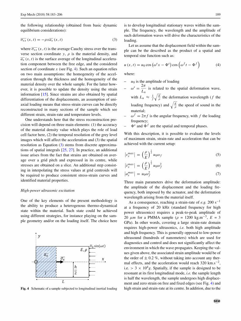
where σxx (x, t) is the average Cauchy stress over the trans-verse section coordinate y, ρ is the material density, andax (x, t) is the surface average of the longitudinal accelera-tion component between the free edge, and the consideredsection of coordinate x (see Fig. 4). Such an equation relieson two main assumptions: the homogeneity of the accel-eration through the thickness and the homogeneity of thematerial density over the whole sample. For the latter how-ever, it is possible to update the density using the straininformation [15]. Since strains are also obtained by spatialdifferentiation of the displacements, an assumption of uni-axial loading means that stress-strain curves can be directlyreconstructed in many sections of the sample which seedifferent strain, strain-rate and temperature levels.

One understands here that the stress reconstruction pre-cision will depend on three main elements: (1) the accuracyof the material density value which plays the role of loadcell factor here, (2) the temporal resolution of the grey levelimages which will affect the acceleration and (3) the spatialresolution as Equation (3) stems from discrete approxima-tions of spatial integrals [25, 27]. In practice, an additionalissue arises from the fact that strains are obtained on aver-age over a grid pitch and expressed in its centre, whilestresses are obtained on a slice. An additional step consist-ing in interpolating the stress values at grid centroids willbe required to produce consistent stress-strain curves andidentified material properties.

High-power ultrasonic excitation

One of the key elements of the present methodology isthe ability to produce a heterogenous thermo-dynamicalstate within the material. Such state could be achievedusing different strategies, for instance playing on the sam-ple geometry and/or on the loading itself. The choice here

Fig. 4 Schematic of a sample subjected to longitudinal inertial loading

is to develop longitudinal stationary waves within the sam-ple. The frequency, the wavelength and the amplitude ofsuch deformation waves will drive the characteristics of theloading.

Let us assume that the displacement field within the sam-ple can be the described as the product of a spatial andtemporal sine function such as:

u (x, t) = u0 cos(ωsx − s

)cos

(ωf t − f

)(4)

where:

– u0 is the amplitude of loading

– ωs = 2π

Ln

is related to the spatial deformation wave,

with Ln ≈ 1f

√Eρthe deformation wavelength (f the

loading frequency) and√

Eρthe speed of sound in the

material;– ωf = 2πf is the angular frequency, with f the loading

frequency;– s and f are the spatial and temporal phases.

With this description, it is possible to evaluate the levelsof maximum strain, strain-rate and acceleration that can beachieved with the current setup:

∣∣εmaxx

∣∣ =( ρ

E

) 12u0ωf (5)

∣∣εmaxx

∣∣ =( ρ

E

) 12u0ω

2f (6)

∣∣amaxx

∣∣ = u0ω2f (7)

Three main parameters drive the deformation amplitude:the amplitude of the displacement and the loading fre-quency, both imposed by the actuator, and the deformationwavelength arising from the material itself.

As a consequence, reaching a strain-rate of e.g. 200 s−1

at a frequency of 20 kHz (standard frequency for highpower ultrasonics) requires a peak-to-peak amplitude of20 μm for a PMMA sample (ρ = 1200 kg.m−3, E = 3GPa). In other words, covering a large strain-rate domainrequires high-power ultrasonics, i.e. both high amplitudeand high frequency. This is generally opposed to low-powerultrasound (hundreds of nanometers) which are used fordiagnostics and control and does not significantly affect theenvironment in which the wave propagates. Keeping the val-ues given above, the associated strain amplitude would be ofthe order of ± 0.2 %, without taking into account any ther-mal effects, and the acceleration would reach 320 km.s−2,i.e. > 3 × 104g. Spatially, if the sample is designed to beresonant at its first longitudinal mode, i.e. the sample lengthis half the wavelength, the sample undergoes high displace-ment and zero strain on free and fixed edges (see Fig. 4) andhigh strain and strain-rate at its centre. In addition, due to the

190 Exp Mech (2018) 58:183–206

viscoelastic dissipation, the central part of the sample willheat up cycle after cycle, while the edges will remain almostat room temperature. The last point is due to the significantmismatch between the characteristic conduction time withina PMMA sample [12] and the loading frequency, providingadiabatic conditions during loading.

The above shows that it is possible to reach large strain-rates in the material, of the order of hundreds of s−1,with a heterogeneous state of strain, strain-rate and tem-perature which enables to test the material over a widerange of thermo-mechanical conditions within a single test.The present article aims at demonstrating the experimen-tal feasibility of this idea and at providing initial results onPMMA.

Results and Discussion

Presentation of the Results

A single PMMA sample was submitted to the experimen-tal procedure detailed above (see “Experimental Procedureand Data Processing”). Successive sequences of grey levelimages were captured while the temperature was continu-ously recorded until the sample reached its glass transitiontemperature. The test was composed of two series of suc-cessive ultrasonics runs. In the first series, six ultrasonicruns were successively applied to the sample at low power,leading to a maximum strain of ± 735 μdef. It was thenfollowed by five other runs at a higher actuator power, lead-ing to a maximum strain of ± 1542 μdef. Between both testseries, the sample was allowed to cool down back to roomtemperature.

Figure 5 presents the temperature record at the highestpower (2nd series). The red lines show the different instantswhen short ultrasonic runs were applied (shaded region inFig. 3) and the map shows how the sample temperature pro-file (averaged over the sample width) evolves as a functionof time. During each loading (800 ms), the sample rapidlyheated up (within the red line) and then cooled down untilthe next run. Figure 5 shows this cooling process with aslight decrease in temperature between two red lines. Only4 s before and after each ultrasonic loading are shown onthe figure. Black dots symbolize the skipped IR frames.

Figure 6 shows the evolution of the measured longitudinaldisplacement, strain, strain-rate and reconstructed stress pro-files as a function of time. The data corresponds to the firstultrasonic run at higher strain amplitude (2nd series), i.e.within the first red line in Fig. 5. As stated in “Experimentand Data Processing”, the data at a given time step is rep-resented as a 1D signal, therefore, Fig. 6 shows space vstime plots. These maps evidence that the sample is indeedloaded on its first longitudinal deformation mode, since

Fig. 5 Temperature profiles (along sample length) as a function oftime during the second ultrasonic test series. Red lines are loadinginstants while the black dots are used to symbolize the delay betweenloading instants

stationary and half wavelength waves can be observedduring the 256 μs captured by the camera. The sampleundergoes a cyclic displacement of ± 25 μm, cyclic defor-mation of ± 1500 μdef, cyclic strain-rate of about ± 200s−1 and a cyclic stress of about ± 7 MPa. Regarding Fig. 5,the sample undergoes also a local increase of temperatureup to 110 ◦C at the end of the test while the sample edgesremains close to room temperature. The following thermo-mechanical fields are consistent with the analytic estimatespresented in “High-power ultrasonic excitation” and con-firm the heterogeneity of the thermodynamical state withinthe material.

Going down into the detail of each ultrasonic run, Fig. 7presents the strain, strain-rate and stress amplitude profiles(half peak-to-peak) as well as the temperature profiles forevery successive ultrasonic loading. Such profiles are com-puted by calculating, for each sample section, half of thepeak-to-peak amplitude over 5 ultrasonic cycles (see Fig. 6)for each of the 11 successive ultrasonic runs. Apart fromvisualisation, the following data is used to define the valueof the apparent strain-rate per sample section. Indeed, eachsection undergoes a cyclic load and thus, a range of strain-rates. Nevertheless, as it is usually assumed in standardDynamic and Mechanical Analysis, for a sake of simplicity,the time variation can be collapsed into a single appar-ent strain-rate value defined here as half the amplitude ofstrain-rate seen by each section. The consequences of thisassumption are discussed further in “Outstanding Issuesand Scope of The Method”. Finally, the frame-rate of theIR camera does not allow a temporal description of thetemperature field over each cycle. As a consequence, each

Exp Mech (2018) 58:183–206 191

Fig. 6 Displacement, strain,strain-rate and stress as afunction of time. The data havebeen averaged across thespecimen width. The datacorresponds to the 1st verticalred line in Fig. 5

(a) displacement (b) strain

(c) strain-rate (d) stress

temperature profile presented in Fig. 7(d) only results froma single frame. The strain and strain-rate data close to thefree and fixed edges have been discarded because of edgeartefacts from the Gaussian smoothing of the displacementfields. It is also important to note that the temperatures over90 ◦C (see dashed rectangle in Fig. 7(d)) have been recon-structed using cubic spline interpolation. Indeed, due to thechosen integration time, the camera sensor saturated above90 ◦C. An integration time of about 400 μs or a multi-ITstrategy would have been more suitable to capture the range[25 - 110] ◦C.

One observes that, when the sample is loaded at ± 735μdef (1st series), the strain amplitude varies continuouslyalong the sample length from 400 to 735 μdef, the strain-rate amplitude from 50 to 115 s−1, the stress amplitude from

0.2 to 4 MPa, and the temperature slightly increases in thesample centre from 23.3 to 34.6 ◦C while the edges remainsat room temperature.

When the sample is loaded at ± 1542 μdef (2nd series),the strain amplitude varies from 200 to 1542 μdef, thestrain-rate amplitude from 40 to 220 s−1, the stress ampli-tude from 0.2 to 7.6 MPa, and the temperature increasesin the sample centre from 23.4 to 105 ◦C. Contrary to thefirst test series where all curves overlapped almost perfectly,the second series evidences a softening of the material asdemonstrated on Fig. 7(c). This is due to significant increaseof the temperature cycle after cycle (see Fig. 7(d)). A clearchange of the material response can be observed at the4th and 5th ultrasonic runs. These two loading cases arecharacterized by a significant drop of the stress down to 6

192 Exp Mech (2018) 58:183–206

Fig. 7 Strain, strain-rate, stressand temperature profiles (alongsample length) for eachultrasonic run. The free edge isat 0 mm while the fixed edge isat 55 mm

(a)

(c) (d)

(b)

then 3 MPa as well as clear change in the profile shapes.Indeed, one can see on Fig. 7(a) a clear strain localiza-tion in the sample centre and a significant decrease of thestrain level everywhere else. These phenomena are due toa sharp localized change in the stiffness of PMMA dueto glass transition. The phenomenon starts at the 4th run,i.e. around 95 ◦C but leads a clear collapse of the materialstiffness at the 5th run, i.e. around 105 ◦C. Such a drasticlocal change in material property also leads to a signifi-cant change in the deformation mode of the sample. Indeed,while the material is initially perfectly tuned to be resonanton its first longitudinal mode at 20 kHz, one observes a sig-nificant decrease of the wavelength (see Fig. 7(c)) at the 4th

and 5th runs. This point is the reason why finite differenceshave been used to obtain experimental acceleration fields asthe assumption of homogeneous material response cannotbe ensured anymore. According to the wavelength formu-lation, available in “Theoretical Framework”, a decrease ofthe wavelength relates to a drop of the stiffness which willbe evidenced further. In the present case, the temporal reso-lution (50 Hz) of the temperature signal combined with theheating rate does not allow finely capturing the Tg , but a

value around 100 ◦C is reasonably in line with glass tran-sition temperatures measured on the material using DMTA(see Table 1).

The data can now be combined to identify the materialproperties as a function of temperature and strain-rate.

Storage Modulus and Damping Identification

Figure 8 presents the evolution of the material responsewithin three different sample cross-sections (at ε = ± 1542μdef, i.e. test series 2 - cf. Fig. 7) and for different ultra-sonic runs. The dots represent the experimental data whilethe curves are based on a sinusoidal least-square fit. Bothstress and strain are temporally fitted by a sine function asfollows:

εf (x, t) = α0sin(2πf t + φ0) (8)

σf (x, t) = α1sin(2πf t + φ1) (9)

where f is the loading frequency, t is the time, x is theaxial position and αi and φi are the amplitudes and phasesof strain and stress for i=0 and i=1 respectively. From this

Exp Mech (2018) 58:183–206 193

Fig. 8 Stress-strain curves for 3different sample sections, fromfree edge to sample centre, andfor different ultrasonic runsduring the 2nd test series, i.e.high strain-rate amplitude

(a) (b)

(c) (d)

description, tan(δ) can also be obtained from the temporalphase shift between the stress and the strain as follows:

tan(δ)(s, t) = tan(φ0 − φ1) (10)

This parameter is widely used to describe the damping ofthe material. The real part of Young’s modulus, the storagemodulus, is then identified from the ratio α1

α0cos (δ).

The results show a number of important trends. Look-ing at Fig. 8(a) of the first run when the temperature in thespecimen is still uniform (see Fig. 7(d)), one can see thatthe central sections provide a stiffer response than the out-ward one. This is the stiffening effect of strain-rate. Basedon the data in Fig. 7(b), the material at 10 mm experiencesa strain-rate of about 50s−1 while the centre responds undera strain-rate of about 80s−1. Both stiffness and strain-ratecontrasts are not very large but the effect is significant. Thesecond trend is the effect of temperature, which is muchmore prominent for this test. As the runs progress and thetemperature increases at the centre of the sample, the stiff-ness drops as clearly seen in Fig. 8(c) and consistently overthe whole test series. Finally, it is also clear from Fig. 8 thatas the temperature increases, the hysteresis loops open up,indicating an increase in damping.

Based on the following local stress-strain relationships,the storage modulus and tan(δ) have been identified and theresults are presented in Fig. 9. Figure 9(a) presents the vari-ation of storage modulus as a function of strain-rate andtemperature. The red dots are the experimental data pointsobtained by combining information over 42 material sec-tions (55 lines minus two filtering kernels to discard edgesartefacts) and eleven ultrasonic runs, i.e. 462 data points.It is important to understand that each material slice istreated independently of its neighbours as if this was a sep-arate material test. The continuous colour map is obtainedby interpolating the data between the red dots using theMatlab� embedded natural neighbour interpolation methodbased on Voronoi tessellation. The figure shows the range ofthe current experiment, i.e. strain-rates between 30 and 220s−1 and temperatures between about 25 and 105 ◦C. Withinthis 2D loading condition space, the storage modulus variesfrom 1.5 GPa, at high temperature, up to 6.3 GPa at lowtemperature. The experiment clearly captures the tempera-ture sensitivity of PMMA with a strong vertical gradient inthe map in Fig. 9(a). Looking at the isothermal curves (hor-izontal gradient), a slight strain-rate sensitivity can also benoticed, as expected. This effect is small however as thestrain-rate range covered here is rather small. One can also

194 Exp Mech (2018) 58:183–206

Fig. 9 Identification of storagemodulus and tan(δ) as a functionof strain-rate and temperature.

(a) (b)

observe higher noise on the data for the lower strain-rateand temperature ranges. This corresponds to sections closeto the specimen edges where both stress and strain are lowerand therefore, exhibit degraded signal to noise ratios.

Then, Fig. 9(b) presents the variation of the tan(δ) param-eter which is associated to the material damping. A fewexcessively high and unrealistic damping values have beendiscarded (less than 10 data points higher than 0.4) and thecolormap saturates at 0.3 to visually capture the local gradi-ents. The same trend as for the storage modulus is observed,although the data are noisier. This was expected as tan(δ)derives from small fractions of the total stress and strain. Asfor the storage modulus, the noise is larger in the low tem-perature and low strain-rate range, for the same reason. It isinteresting to compare these data to that available in the lit-erature. Looking for instance at [18], the variation of tan(δ),from ambient to 105 ◦C, ranges between about 0.03 and 0.3which is the range also observed here. Another interestingobservation is that there is a trend for higher values at lowstrain-rate and temperature. This may be related to the pres-ence of a β-transition around room temperature, but the poorsignal to noise ratio there precludes any definite conclusion.More tests are needed to explore this part of the temperature/ strain-rate space.

From a technical point of view, both graphs evidence avery heterogeneous data-point density. Indeed, Fig. 9(a) hasa large significant data-point density between 50 and 100s−1 for temperature comprised between ambient and 35 ◦Cwhereas very few data-points are available at higher temper-ature. This point is not intrinsic to the method and mainlydepends on the chosen ultrasonic loading amplitudes. In thepresent work, only two amplitude steps have been used (±735 μdef and ± 1542 μdef). Using more steps would haveled to a more homogeneous space sampling.

Finally, time temperature superposition has been used inan attempt to collapse all the data in Fig. 9(a) on a single master

curve. To achieve this, experimental data points undergoinglow strain-rates (< 70 s−1, see “Finite Element Validation”for details), and the ones close to Tg and post Tg have beendiscarded. For the latter, as the glass transition was not iden-tified accurately, the procedure has consisted in removingdata over a threshold damping value of 0.3 (see top yellowregion in Fig. 9(b)) and a threshold temperature value of95 ◦C.

For thermo-rheologically simple materials, i.e. materialsthat obey time-temperature superposition which is the caseof PMMA below the Tg , it is assumed that an increase intemperature is equivalent to a decrease in strain-rate. Thereconstruction of a master curve consists therefore in shift-ing isothermal storage modulus curves along the strain-rateaxis by a factor aT until a single curve is obtained, repre-senting the evolution of the material behaviour at a fixedreference temperature T . The shifting factor aT can bedescribed by the Arrhenius equation as follows:

aT (T ) = exp

(�H

R

(1

T− 1

T0

))(11)

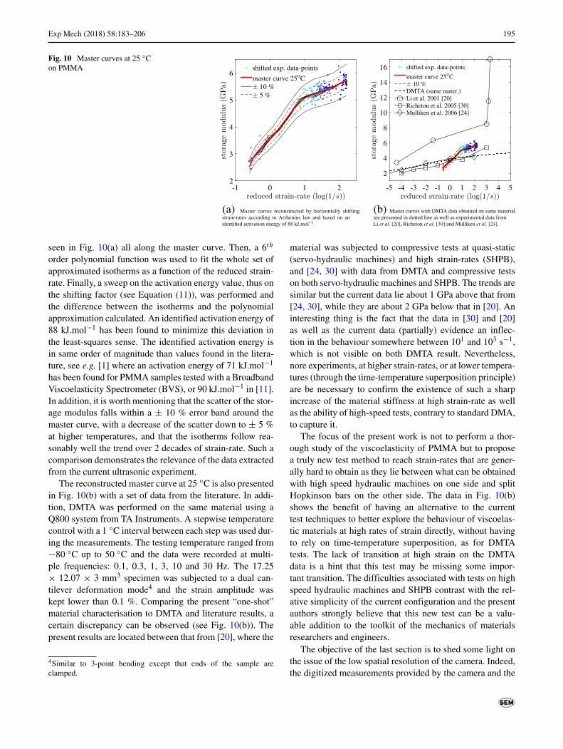
where �H is the activation energy associated with mech-anisms of internal friction, R = 8.3144598 J.mol−1.K−1 isthe gas constant, and T0 is a chosen reference temperature.Figure 10(a) shows the identified master curve at 25 ◦C.Storage modulus values are presented with scattered points(from blue (ambient) to red (hot)). Individual slopes of stor-age modulus isothermal curves are presented with multiplestraight black lines and the master curve and its ± 5 % and± 10 % vertical shifts are presented with plain and dot-ted lines respectively. In practice, to obtain such a mastercurve, storage modulus isothermal curves (horizontal slicesin Fig. 9(a)) were first individually fitted by affine func-tions in order to obtain a first order description of theirslopes. Such set of approximated isothermal curves can be

Exp Mech (2018) 58:183–206 195

Fig. 10 Master curves at 25 ◦Con PMMA

(a) Master curves reconstructed by horizontally shiftingstrain-rates according to Arrhenius law and based on anidentified activation energy of 88 kJ.mol−1.

(b) Master curves with DMTA data obtained on same materialare presented in dotted line as well as experimental data fromLi et al. [20], Richeton et al. [30] and Mulliken et al. [24].

-5 -4 -3 -2 -1 0 1 2 3 4 5

2

4

6

8

10

12

14

16 shifted exp. data-points

master curve 25oC 10 %

DMTA (same mater.)Li et al. 2001 [20]Richeton et al. 2005 [30]Mulliken et al. 2006 [24]

seen in Fig. 10(a) all along the master curve. Then, a 6th

order polynomial function was used to fit the whole set ofapproximated isotherms as a function of the reduced strain-rate. Finally, a sweep on the activation energy value, thus onthe shifting factor (see Equation (11)), was performed andthe difference between the isotherms and the polynomialapproximation calculated. An identified activation energy of88 kJ.mol−1 has been found to minimize this deviation inthe least-squares sense. The identified activation energy isin same order of magnitude than values found in the litera-ture, see e.g. [1] where an activation energy of 71 kJ.mol−1

has been found for PMMA samples tested with a BroadbandViscoelasticity Spectrometer (BVS), or 90 kJ.mol−1 in [11].In addition, it is worth mentioning that the scatter of the stor-age modulus falls within a ± 10 % error band around themaster curve, with a decrease of the scatter down to ± 5 %at higher temperatures, and that the isotherms follow rea-sonably well the trend over 2 decades of strain-rate. Such acomparison demonstrates the relevance of the data extractedfrom the current ultrasonic experiment.

The reconstructed master curve at 25 ◦C is also presentedin Fig. 10(b) with a set of data from the literature. In addi-tion, DMTA was performed on the same material using aQ800 system from TA Instruments. A stepwise temperaturecontrol with a 1 ◦C interval between each step was used dur-ing the measurements. The testing temperature ranged from−80 ◦C up to 50 ◦C and the data were recorded at multi-ple frequencies: 0.1, 0.3, 1, 3, 10 and 30 Hz. The 17.25× 12.07 × 3 mm3 specimen was subjected to a dual can-tilever deformation mode4 and the strain amplitude waskept lower than 0.1 %. Comparing the present “one-shot”material characterisation to DMTA and literature results, acertain discrepancy can be observed (see Fig. 10(b)). Thepresent results are located between that from [20], where the

4Similar to 3-point bending except that ends of the sample areclamped.

material was subjected to compressive tests at quasi-static(servo-hydraulic machines) and high strain-rates (SHPB),and [24, 30] with data from DMTA and compressive testson both servo-hydraulic machines and SHPB. The trends aresimilar but the current data lie about 1 GPa above that from[24, 30], while they are about 2 GPa below that in [20]. Aninteresting thing is the fact that the data in [30] and [20]as well as the current data (partially) evidence an inflec-tion in the behaviour somewhere between 101 and 103 s−1,which is not visible on both DMTA result. Nevertheless,nore experiments, at higher strain-rates, or at lower tempera-tures (through the time-temperature superposition principle)are be necessary to confirm the existence of such a sharpincrease of the material stiffness at high strain-rate as wellas the ability of high-speed tests, contrary to standard DMA,to capture it.

The focus of the present work is not to perform a thor-ough study of the viscoelasticity of PMMA but to proposea truly new test method to reach strain-rates that are gener-ally hard to obtain as they lie between what can be obtainedwith high speed hydraulic machines on one side and splitHopkinson bars on the other side. The data in Fig. 10(b)shows the benefit of having an alternative to the currenttest techniques to better explore the behaviour of viscoelas-tic materials at high rates of strain directly, without havingto rely on time-temperature superposition, as for DMTAtests. The lack of transition at high strain on the DMTAdata is a hint that this test may be missing some impor-tant transition. The difficulties associated with tests on highspeed hydraulic machines and SHPB contrast with the rel-ative simplicity of the current configuration and the presentauthors strongly believe that this new test can be a valu-able addition to the toolkit of the mechanics of materialsresearchers and engineers.

The objective of the last section is to shed some light onthe issue of the low spatial resolution of the camera. Indeed,the digitized measurements provided by the camera and the

196 Exp Mech (2018) 58:183–206

grid method are a spatially filtered version of reality and theonly way to understand the effect of this filter on the qualityof the identification is through numerical simulation.

Finite Element Validation

The purpose of this section is to validate the current experi-mental choices by understanding how experimental param-eters such as the camera spatial resolution, the acquisitionfrequency, the grid sampling, the camera sensor noise andthe sensitivity of the algorithm used to recover deforma-tions can affect the precision of the identification. The ideais also to propose some guidelines to the reader and makethis new technique more accessible. The main concern isthe poor camera spatial resolution (400 × 250 pixels) sothis validation is essential to give confidence to the previousresults.

Finite Element Model

The Finite Element (FE) simulation consisted in an 3Dharmonic analysis achieved using the ANSYS 16.2 FEpackage. Thanks to the problem symmetry, only a quarter ofthe sample was modelled. The model was meshed using 0.1mm3 SOLID186 quadratic elements and a harmonic loadingof amplitude 30 μm was applied to the right-hand side edgeof the model (see Fig. 11).

The material was modelled using an isotropic, homoge-neous and purely elastic material. In other words, the presentFE investigation does not deal with the impact of materialtime-dependence, i.e. impact of temperature and strain-ratevariations along the sample length, nor the dissipation, onthe identification validation process. This was found rea-sonable as a first step to quantify the effect of the cameraspatial resolution on the measured and identified quantities.The main characteristics of the FE model are summarizedin Table 2.

Figure 11 shows an example of an FE longitudinal dis-placement field extracted at the top surface of the model andthen symmetrized along the transversal direction.

Fig. 11 Example of FE displacement field extracted at the top surfaceof the FE model and symmetrized along the transverse direction

Synthetic Grid Deformation

The procedure used to evaluate the accuracy of the identifi-cation on real data is presented here. First, the sample defor-mation was simulated with the FE model described above.Then, synthetic grid images were numerically deformedusing the FE displacements fields, grey level noise wasadded and the images were processed exactly as the experi-mental ones (see “Theoretical Framework”). The identifiedparameters can then be compared to the FE inputs and bothsystematic and random errors can be evaluated. A similarapproach can be found in [32, 33, 38].

Synthetic and pixelated grids have been generatedaccording to the following equation:

G(i, j) = γ

4

(1 + cos(2π

i

N)

) (1 + cos(2π

j

N)

)+ γ

(12)

with G is the pixelated grid, N is the spatial sampling(number of pixels per period) and γ and γ characterisesthe image dynamic range (see Fig. 12). A specific gridpitch p was also chosen to scale the image. In parallel, FEdisplacement fields were output from ANSYS and interpo-lated on the grid-mesh using a cubic spline interpolation.Such an interpolation is required to deform the grid usingstandard MATLAB libraries such as the interp2 function.Finally, the grid was numerically deformed, assigning atgrid location M(i, j) an average of the grid grey level valuearound the location M ′(i + u, j + v) where u and v are thelongitudinal and transversal FE displacement at that pixellocation, respectively. Additional spline interpolations wererequired here to estimate the grey level value at locationsM ′(i + u, j + v) and M ′(i + u ± ε, j + v ± ε), where ε ishalf the averaging window size. It corresponds to the fieldof view captured by one pixel of the camera, denoted pix,and allows taking into account the fact that a camera pixelonly captures an average of the grid grey level over a cer-tain physical domain. Here, this window was taken so that itcovers the full pixel size, effectively simulating a fill factorof 100 %, while the Shimadzu HPV-X camera has a low fillfactor, of the order of 40 %. Nevertheless, it was checkednumerically that this effect could be neglected thanks to thevery small recorded displacements (less than a third of apixel), justifying the use of a 100 % fill factor here for thesake of simplicity and computing efficiency. Finally, a greylevel Gaussian noise of standard deviation σ was added tothe grid image to take into account the characteristic noise ofthe camera sensor. Such routine is applied to the initial gridimage for different loading increments until reconstructing127 synthetically deformed and noisy grid images compa-rable to the data set captured by the camera during a realexperiment.

Exp Mech (2018) 58:183–206 197

Table 2 FE model parametersGeometry dimensions (mm) 55 x 6 (sym.) x 2 (sym.)

Mesh size (mm3) 0.1

element SOLID186

Material density (kg.m−3) 1160

Young’s modulus (GPa) 5.5

Poisson’s ratio 0.34

Loading type disp.

amplitude (μm) 30

frequency (kHz) 20

Analysis FE package ANSYS 16.2

type harmonic / full

solver Jacobi Conjugate Gradient itera-tive equation solver

num. damping (s) × 10−7

Figure 12(c) shows a zoomed in image of an experi-mental grid image and Figs. 12(a) and (b) the grey levelhistogram and noise characteristics of the camera sensor.Figure 12(c) shows a zoom in of the synthetic grid afterapplying deformation and noise. The noise added to thesynthetic images is based on Fig. 12(b) where the stan-dard deviation of the pixel noise (obtained from stationaryimages) for different pixels from dark to bright is plotted.

The maximum noise was about 3.5 % of the pixel grey leveland decreases as a function of the grey level intensity. Thegrid contrast has been selected to reproduce the histogramof Fig. 12(a). Comparing Fig. 12(c) and (d), one can notethat the procedure detailed above describes reasonably wellthe grey level dynamic and the noise intensity. However, theprocedure does not take into account any grid defect and anyfill-factor issues. Indeed, one observes in Fig. 12(c) that the

Fig. 12 Experimental imagescharacteristics a), b) and zoomin views of an experimental andsynthetic grid. Thecorresponding parameters are: p= 1 mm, N = 7 mm, pix = 143μm and σ = 3.5 %

(a) (b)

(d)(c)

198 Exp Mech (2018) 58:183–206

Fig. 13 Spatio-temporaldisplacement error maps. On theleft column is the absolute valueof the relative error and on theright column is the absolutevalue of the extracted randompart. The correspondingparameters are: p = 1 mm, N =7 mm, pix = 143 μm, σ = 3.5% and smoothing kernel s = 7

(a) (b)

(d)(c)

apparent pitch of the grid slightly varies along the horizontaldirection. This is due to the fact that the pixel captures pho-tons only over a small part of its physical domain (40 % forthe HPV-X) which leads to a crop of the information espe-cially visible in presence of sharp edges. Both these aspectshave been neglected here.

Before analysing the impact of the grid and cameraparameters on the field reconstructions, one needs to choosea definition for the systematic and random errors, i.e. scalarsaccurately describing spatio-temporal deviations betweeninput and output fields. The idea was to overcome two majorproblems: (1) the presence of infinite values in the defini-tion of the relative error. It comes from the point-by-pointdivision of the output fields by the input ones, of which thelocal values can be null. (2) By smoothing the reconstructeddisplacement field, the random noise will be mitigated butoutputs are more and more truncated which introduces lowspatio-temporal frequency variations within the error. This

makes it difficult to simply define the random error by thestandard deviation of the relative error. The following twopoints are illustrated in Fig. 13 where the relative error ondisplacement fields (see Equation (13)) and its random part(see Equation (14)) are presented for a simulated cameranoise of 3.5 % with smoothing (Fig. 13(c) and (d)) or with-out (Fig. 13(a) and (b)). As expected, singular values closeto the anti-node (sample centre) are present as well as forcertain times when the signals go through zero. One cansee the reduction of high frequency scatter when smooth-ing (from top to bottom) but also the creation of systematiclow-spatial frequency variations (see Fig. 13(c)). Based onthese observations, it has been decided to define the sys-tematic error, denoted εsyst , as the median (over space andtime) of the relative error field as the median is less sensi-tive to outliers arising from low signal points. The randomerror, denoted εrand , is defined as the standard deviation(over space and time) of the difference between the FE data

Exp Mech (2018) 58:183–206 199

corrected by the systematic error and the FE-grid data, nor-malized by the maximum of the signal in space and time. Inequation format:

εsyst = Md

[F FE(x, t) − F grid(x, t)

F FE(x, t)

](13)

εrand = s

[F FE(x, t)

(1 − εsyst

) − F grid(x, t)

maxx,t (F FE(x, t))

]

(14)

where F FE and F grid are the FE (input) and post-processed(output) quantities of interest, Md [∗] and s [∗] are themedian and the standard deviation respectively. For the erroron Young’s modulus, the time has been removed from Equa-tions (13) and (14) to calculate the error, as it does notdepend on time.

Let us now look into the impact of the experimental spa-tial grid sampling, the temporal sampling and the camerasensor noise on measurements and identification. First, fourdifferent spatial grid pitches have been tested, namely p =0.7, 0.8, 0.9 and 1 mm, and the error on kinematic quan-tities evaluated. No clear impact on the systematic error ofdisplacement and strain has been identified since an error of0.5±0.1% on both displacement and strain has been foundwhatever the grid pitch. Therefore, the grid pitch chosenexperimentally, 1 mm, has negligible impact on the dis-placement and strain. The reason for this is certainly thelow spatial frequency contents of the deformation whenthe material undergoes deformation at its first longitudinalmode. Deforming the material at higher deformation modes,or using a strain concentrator like a notch or a hole, wouldrequire to run this check again.

Then, five different frame rates have been used, namelyf = 0.2, 0.5, 1, 2 and 5 Mfps, on a 1 mm pitch grid. Table 3summarizes the results.

One observes that only the 0.2 Mfps frame rate signif-icantly affects the results. Indeed, an error of about 12 %is found for simulation recorded at 0.2 Mfps, while only1-2 % of error was found for higher frame rates. This con-firms the choice of 0.5 Mfps for the experiments, and also

Table 3 Systematic error (in %) between FE and synthetic grid defor-mation data, for different frame rates. The grid pitch is 1 mm and thedisplacement amplitude is ± 30 μm

Frame rate (Mfps)

0.2 0.5 1 2 5

Accel. (finite diff.) 11.6 0.9 0.7 1.1 1.2

Accel. (harm.) 0.3 →Stress (finite diff.) 11.4 0.7 1.0 1.7 1.9

Stress (harm.) 0.14 →Young’s modulus (finite diff.) 12.3 1.9 0.3 0.5 1.2

Young’s modulus (harm.) 0.5 →

shows that a slight improvement would have been obtainedrecording at 1 Mfps or more. It is interesting to notice thatthe small unexpected increase of the identification errorover 1 Mfps is probably due to the fact that the system-atic errors presented here are based on spatio-temporal dataobtained considering a constant number of frames capturedby the camera (128) and not considering a constant numberof deformation cycles. This has been chosen to be in linewith the physical limitation of the camera. In other words,when an increase of the acquisition frequency is simulated,a decrease of the number of captured deformation cyclesoccurs. At 1 Mfps, two and a half cycles are captured, at 2Mfps only one and at 5 Mfps, only half of a cycle. There-fore, increasing the frame rate affects the consistency ofthe comparison and probably slightly increases the system-atic error. However, this error still remains very small. Thetable also shows that avoiding temporal differentiation byusing the harmonic assumption leads to lower errors on theacceleration and stress, as expected.

Finally, a noise level of 3.5 % was added to the syntheti-cally deformed grid images, each of the 128 images bearinga different copy of the noise. Table 4 and Fig. 14 presenthow displacement smoothing affects the strain, acceleration,stress and identified Young’s modulus. For comparison,Fig. 13 provide the error fields corresponding to the firstrow, column one and two in Table 4. The first column ofTable 4 shows the level of noise before any post-smoothing.No systematic error is observed but a significant randomerror can be seen on differentiated quantities, especiallythe strain and the acceleration with a noise standard devi-ation of about 11 % and 13 %, respectively. One can seethat the random error level is only about 6 % on stress(finite diff.). This point is in line with the fact that thestress comes from averaging the acceleration between eachmaterial section and the free edge. This is a regularizing pro-cess. In addition, one observes that the harmonic assumption

Table 4 Systematic and random errors (in %) between FE andsynthetic grid deformation data.

no smoothing smoothed k = 7

Displacement 0.2±1.7 6.7±0.6

Strain 0.4±11.0 6.7±2.7

Acc. (finite diff.) 0.6±12.9 7.2±1.5

Acc. (harm.) 0.2±1.7 6.7±0.6

Stress (finite diff.) 0.1±5.7 7.0±1.2

Stress (harm.) 0.2±1.0 6.6±0.8

Young’s modulus (finite diff.) 2.8±3.1 1.4±1.8

Young’s modulus (harm.) 1.5±3.2 0.8±1.8

The image noise was 3.5 % of the grey level value and thedisplacement amplitude ± 30 μm. Smoothing was Gaussian withkernel k, in space for strains, and in time for acceleration(finite difference). Data provided as systematic±random error

200 Exp Mech (2018) 58:183–206

(a) (b) (c)

(d) (e)

(g) (h)

(f)

Fig. 14 Systematic and random errors (in %) between FE and synthetic grid deformation data. The image noise was 3.5 % of the grey level valueand the displacement amplitude ± 30 μm

significantly mitigates the influence of the noise. Both har-monic acceleration and stress have a level of noise similarto the displacement one. Finally, one can see that the identi-fied Young’s modulus has a systematic error which is abouttwice as large when using finite differences instead of theharmonic assumption to derive the acceleration. The latteris therefore favoured, as expected.

Table 4, column two, focuses on the smoothing kernelsize selected for the treatment of the experimental data. Akernel size of 7 was applied in space to derive the strains,and in time to derive the acceleration using finite differ-ences. Two things can be noticed: first, smoothing the dataintroduces a systematic error of the order of 7 % for allquantities except the identified Young’s modulus. Second, itsignificantly reduces the random error for the differentiated

quantities, i.e. the strain (-8 %), the acceleration (-11 %)and the stress (-4.5 %). As expected, the random error doesnot reduce significantly on acceleration and stress whenusing the harmonic assumption, the smoothing just increas-ing the systematic error. The situation for Young’s modulusis somewhat unexpected as not only does the random errordecrease, as expected, but also the systematic error by afactor of two. This comes from the fact that both stressand strain systematic errors cancel out when the modulus iscalculated. Whether this is a general result or just a fortunatefact arising from the precise set of smoothing parametersused here remains to be confirmed.

Finally, Fig. 14 shows the variation of the systematicand random errors when the smoothing kernel size varies.For all quantities, the systematic error increases when the

Exp Mech (2018) 58:183–206 201

smoothing kernel increases and the random error decreaseswhen the kernel increases, as expected. This allows to selectthe smoothing in a rational way to minimize the total error,as in [38]. It is clear from Fig. 14(b), (c) and (e) that a smooth-ing kernel between 5 and 7 is recommended. Regarding theidentified Young’s modulus, it is interesting to notice that thetrend of the systematic error is almost flat whereas the system-atic error on both strain and stress increases as a function ofsmoothing kernel size. It means that the systematic errorson both stress and strain increase in similar ways and can-cel out in the Young’s modulus identification. This specificpoint means that depending on the purpose of the study,i.e. identifying a material parameter or measuring accuratelymechanical quantities, the choice of the smoothing kernelwill not necessarily be the same. In parallel, one observesthat the random error on Young’s modulus identificationsignificantly decreases over a smoothing window of 5. Nev-ertheless, none of the tested parameters allow reaching anerror level below 1 %. A wider range of smoothing and gridparameters would be needed to better understand this, butthis was beyond the scope of the present validation whichfocuses on evaluating the expected error for the parametersused in the experimental study. These results also demon-strate the benefit of the synthetic image deformation processto gain insight into the errors than can be expected on theidentified quantities, as already pointed out in [32, 33, 38].

To conclude, Fig. 15 presents the relative error expectedon Young’s modulus identification for the experimental con-ditions presented in “Results and Discussion”, i.e. a gridpitch of 1 mm, a frame rate of 0.5 Mfps, a flat camerasensor noise across pixel grey level values of 3.5 % and adata post-smoothing kernel of 7 prior to both spatial andtemporal differentiation. In view of the simplifications in theFE model, in particular the fact the material does not includeany viscoelastic effects, i.e. no Young’s modulus variationsalong the sample length are present, the results can be seen

as a lower bound of the identification error. Figure 15(a)presents the relative error on the identified Young’s modulusall along the sample length. The dotted red line representsthe median value already reported in Table 4. One observes a3 % oscillation of the identified Young’s modulus along thesample length, from 10 to 40 mm. Between 5 and 10 mm,and 40 and 50 mm, oscillations reach 10 %. Close to thefree (0 mm) and the loaded (55 mm) edges, the identifica-tion error shoots up. This is due to the fact that both stressesand strains are zero at the deformation nodes. It is worth not-ing that the sample extremities (one smoothing kernel, i.e. 7data, at both ends) have not been taken into account for theestimation of the systematic and random errors presentedwithin this section. Such a figure shows that the accuracy ofthe identification is not constant over the sample length anddepends on the position of the material section comparedto the deformation nodes and anti-nodes. Indeed, Fig. 15presents a characteristic U shape which derives from thespatial variation of the signal to noise ratio. Here, the spa-tial location can be translated into strain-rate in order tounderline the resulting impact of such signal to noise ratiovariation on the ability to the experiment to characterizemechanical properties at lower strain-rate.

Figure 15(b) presents the relative error on the identifiedYoung’s modulus as a function of the strain-rate ampli-tude seen by each sample section. One clearly sees that therelative error on Young’s modulus starts from 1 % at maxi-mum strain-rate (i.e. sample centre) then gradually increasesas the considered section gets closer to the edges. Withinthe domain [200-250] s−1, the systematic error remainsbelow 2 % and reaches 6 % down to 90 s−1. Below this,Young’s modulus is not identified accurately anymore. Suchobservations are in line with the experimental observations.Indeed, Fig. 10(a) shows an identification scatter about ± 5% at the sample centre (high temperature - high strain-rate)and about ±10 % close to sample edge which is consistent

10 20 30 40 5010-1

100

101

102

(a) Error as a function of sample length

0 50 100 150 200 25010-1

100

101

102

(b) Error as a function of the local amplitude of strain-rate

Fig. 15 Absolute value of the relative error on Young’s modulus identification for a grid pitch of 1 mm, a temporal sampling f = 0.5 Mfps, agrid noise of 3.5 % and a spatio-temporal smoothing kernel size of 72. The material was assumed, isotropic, homogeneous and purely elastic. Thedisplacement amplitude is ± 30 μm and the acceleration was obtained from finite difference. The red line in a) is the median value while the redline in b) underlines the limit (90 s −1) under which the identification error shoots up

202 Exp Mech (2018) 58:183–206

with Fig. 15(b). Moreover, Fig. 15(b) shows that the system-atic error slightly increases close to the sample edges whichcould partially explain the deviation with [30], observed inFig. 10(a) at 102 s−1.

The present data lead to the following conclusions. (1)Combining a spatially heterogeneous loading together withkinematic and temperature full-field measurements, it ispossible to identify Young’s modulus over a certain rangeof thermo-mechanical loading conditions. (2) The accuracyof the local identification strongly depends on experimentalconditions and processing parameter selection, especiallythe sensor noise, the acquisition frequency, the camera res-olution, the grid resolution and the smoothing parameters.Such parameters can be chosen in a rational way by combin-ing finite element modelling and synthetic grid deformation.(3) Nevertheless, with such a ”one-shot” technique, the costto pay is a variation of the signal to noise ratio as a func-tion of spatial location, i.e. also as a function of temperature,strain and strain-rate. Here, the results are acceptable downto strain-rates of 90 s−1 and up to 250 s−1. Deeper inves-tigations using thermo-mechanical viscoelastic simulationsare required to gain better understanding of the metrologicallimitations of the experiment.

Outstanding Issues and Scope of the Method

Although the feasibility of a ”one-shot” time-dependentproperties identification has been demonstrated on a PMMAsample and the results are in good agreement with dataobtained from other methods, such as DMTA and high-speed compressive tests, it is important to understand thelimitations and outstanding issues of the proposed method-ology. A few points need to be raised.

– The difficulty to clearly define an apparent strain-rate. Such difficulty is actually also present in DMTAand SPHB tests but at least the methodologies are con-sistent since data are also averaged in space. In thepresent case, the following issue can introduce a hor-izontal shift of the data in Fig. 9. As the strain-ratefor result reported here is the maximum strain-rate,effective properties may be slightly shifted towardslower strain-rates. One can notice that the convention inDMTA is to approximate the strain-rate by ε = 4f εmax

[24] whereas one uses here εmax , i.e. ≈ 2πf εmax whichwould lead to an horizontal shift of about 0.2 s−1.This is not enough to explain the significant differencesobserved in Fig. 10(b).

– The strain amplitude sensitivity. The strain variesalong the sample length and during the test from 0.01to 0.35 %, which means that the following test is closeto DMTA in term of deformation amplitude (0.1 %) but

somewhere between hydraulic machine tests and SHPBtests in term of strain-rates. The potential impact of thestrain amplitude on the storage modulus variation, espe-cially at low strains, is not clear and could introducesome variation of storage modulus simply due to strainamplitude variations. This point can affect the globalshape of the master curve.

– Limitation of a 1D approach. It has been observed thatthe temperature was not perfectly uniform over a mate-rial section (see supplementary data) due to both higherheat losses at the edges and unsymmetrical strain local-ization. It seems important to investigate how such anapproach could be extended to a 2D case which wouldnot require this assumption. The present authors are cur-rently working on a strategy based on the use of theVirtual Fields Method and a subset-based equilibriumto overcome such an issue.

While the current article focuses on a rather simple appli-cation (a homogeneous rectangular specimen in the elasticregime) as a first demonstrator, the present strategy has greatpotential for a range of problems not addressed with currenttest methods.

1. Fracture of brittle materials at high strain-rate.Brittle materials like glass or concrete are notoriouslydifficult to test at high rates of strain. A preliminarynumerical simulation on glass with a ± 60 μm excita-tion amplitude (limit of the current ultrasonic excitationsystem), and considering a very low damping coeffi-cient of β ≈ 10−9 leads to a maximum stress of σ =±95 MPa, i.e. about the fracture stress of glass. As thematerial is not damped, the actuator can work over itswhole displacement range to reach the failure stress ofglass. Combining such test with a 2D generalization ofthe method would allow characterizing glass failure athigh strain-rates. An initial experimental proof of prin-ciple has been conducted and a glass specimen has beensuccessfully fractured.

2. Transverse fracture of composites. Because of thevery low failure stress of a unidirectional (UD) com-posite in the direction transverse to the fibres, itstensile fracture stress is very difficult to obtain usingSHPB experiments. A preliminary finite element studyshowed that an amplitude of ± 100μm would berequired to reach σ = 50 MPa with E = 10 GPa and β ≈10−8. While this is larger than what the current systemused here can provide, it is not impossible to reach. Analternative could also be to fix a mass at the free end,this would however require a significant numerical testdesign campaign. The situation is even more difficultfor the through thickness tensile properties where verysmall specimens have to be used. In this case, a thinlaminate could be sandwiched between two steel blocks

Exp Mech (2018) 58:183–206 203

and displacement measurements just performed on thesteel blocks with a direct reading to the transverse stressfrom the free end steel block.

3. Adhesives. The same idea as for the through-thicknesscomposites test could be employed for adhesives whichare notoriously difficult to test at high rates [39].

4. Yielding of engineering alloys. From initial finite ele-ment simulations, the actuator would also need anamplitude of ± 160 μm to yield an aluminium sam-ple (with σy = 280 MPa, E = 72 GPa and β ≈ 10−10). Again, this is too large for the current setup but aspecific horn could be designed to boost the excitationamplitude further.

5. Extended strain-rate range. The current strain-raterange is imposed by the excitation frequency, the strainconcentration within the sample and the covered rangeof temperatures (considering time-temperature super-position). It is possible to reach higher apparent strain-rates by cooling down the sample prior to the start of thetest, e.g. building a temperature controlled enclosure.According to preliminary calculations and tests, coolingthe specimen down to 10 ◦C only would allow reachingthe equivalent of 103 s−1 at room temperature, whilecooling down to −10 ◦C would allow reaching 104

s−1 at room temperature for PMMA samples. Work-ing on sample geometry (using notches for instance)would lead to strain concentrations and thus higherlocal strain-rates. Nevertheless, the suitability of the lowspatial resolution camera would need to be verified, andthe 1D approach would most probably not be enough.

6. Heterogeneous materials. Although the present paperuses a simple homogeneous PMMA specimen for thesake of validation of the test concept, it is clear thatthe main asset of this image-based DMTA is to investi-gate heterogeneous materials. Indeed, while a techniquesuch as DMTA is now well mastered and allows cap-turing the behaviour of rheologically simple materialsover a very large range of strain-rates (see Fig. 10(b)), itcannot provide spatial maps of properties and therefore,cannot derive detailed properties for heterogeneousmaterials. An interesting case for instance could beinjected polymeric sheets which have different proper-ties in the skin than in the core. The present method hasthe potential to provide spatially-resolved properties.

These opportunities will be studied in more depth by thecurrent authors in the near future.

Conclusion

The present work demonstrates the feasibility of a multi-parametric identification on a single sample and falls within

an effort to invent new high-strain test methodologies basedon full-field imaging and inverse identification, to bothovercome the limits of standard experimental strategies andtake advantage of the deformation heterogeneities to achievea full-characterization of a material from a “one-shot” test.It has been demonstrated that using a 20 kHz high powerultrasonic excitation combined with infrared thermographyand ultra-high speed imaging, a PMMA sample could besubjected to apparent strain-rates varying from less than 100

s−1 to 102 s−1 and temperatures varying from ambient toits Tg . Within the studied strain-rate range, a significantincrease in storage modulus has been evidenced that wasnot visible in the DMTA results. This interesting observa-tion justifies the interest in developing new measurementtechniques to capture the material behaviour at intermediateand high strain-rates. The validity of the approach has beenchecked using Finite Element modelling combined withsynthetic grid image deformation. It demonstrates, undersimple behaviour assumptions, that the error on identifi-cation is expected to remain below 10% over the samplelength. This has been partially confirmed by the experi-mental data scatter. Finally, the potential of this new testtechnique has been underlined and it is expected that it willevolve to join the toolkit of researchers and engineers inmechanics of materials.

Acknowledgments This material is based on research sponsoredby the Air Force Research Laboratory, under agreement numberFA9550-15-1-0293. The U.S. Government is authorized to reproduceand distribute reprints for Governmental purposes notwithstandingany copyright notation thereon. The views and conclusions containedherein are those of the authors and should not be interpreted asnecessarily representing the official policies or endorsements, eitherexpressed or implied, of the Air Force Research Laboratory or theU.S. Government. The authors would like to thank Dr Jason Foley(AFOSR), Dr Matt Snyder (EOARD) and Dr David Garner (EOARD)for supporting this work.

Prof. Pierron acknowledges funding from EPSRC through grantEP/L026910/1, as well as from the Wolfson Foundation through aRoyal Society Wolfson Research Merit Award.

The authors are also grateful to Prof. Clive Siviour from the Depart-ment of Engineering Science at the University of Oxford for providingthe DMTA results and for helpful discussions.

The authors are also grateful to Dr. Frances Davis from the Engi-neering and the Environment research group from the University ofSouthampton for performing the quasi-static tests, density measurementsand DSC analysis on PMMA samples, as well as for helpful discussions.

All data supporting this study are openly available from the Universityof Southampton repository at http://doi.org/10.5258/SOTON/D0207.

Open Access This article is distributed under the terms of theCreative Commons Attribution 4.0 International License (http://creativecommons.org/licenses/by/4.0/), which permits unrestricteduse, distribution, and reproduction in any medium, provided you giveappropriate credit to the original author(s) and the source, provide alink to the Creative Commons license, and indicate if changes weremade.

204 Exp Mech (2018) 58:183–206

Appendix

Fig. 16 Data post-processing procedure

Exp Mech (2018) 58:183–206 205

References

1. Capodagli J, Lakes R (2008) Isothermal viscoelastic properties ofPMMA and LDPE over 11 decades of frequency and time: a testof time–temperature superposition. Rheol Acta 47(7):777–786

2. Crooks J, Marsh B, Turchetta R, Taylor K, Chan W, Lahav A,Fenigstein A (2013) Kirana: A solid-state megapixel ucmos imagesensor for ultrahigh speed imaging. In: Proceedings of SPIE - theinternational society for optical engineering, volume 8659

3. Dreuilhe S, Davis F, Siviour CR, Pierron F (2016) Image-basedinertial impact tests on an aluminum alloy. In: Conference pro-ceedings of the society for experimental mechanics series, volume3, pages 219–223

4. Dreuilhe S, Pierron F (2015) Extension of the non-linear virtualfields method to inertial heterogeneous high strain rate tests. Con-ference Proceedings of the Society for Experimental MechanicsSeries 4:83–87

5. Field JE, Walley SM, ProudWG, Goldrein HT, Siviour CR (2004)Review of experimental techniques for high rate deformation andshock studies. Int J Impact Eng 30(7):725–775

6. Fruehmann R, Crump D, Dulieu-Barton J (2013) Characterizationof an infrared detector for high frame rate thermography. Meas SciTechnol 24(10):105403

7. Giraudeau A, Pierron F, Guo B (2010) An alternative to modalanalysis for material stiffness and damping identification fromvibrating plates. J Sound Vib 329(10):1653–1672

8. Grediac M, Fournier N, Paris PA, Surrel Y (1998) Direct identifi-cation of elastic constants of anisotropic plates by modal analysis:Experimental results. J Sound Vib 210(5):643–659

9. Grediac M, Paris PA (1996) Direct identification of elastic con-stants of anisotropic plates by modal analysis: Theoretical andnumerical aspects. J Sound Vib 195(3):401–415

10. Grediac M, Sur F, Blaysat B (2016) The grid method for in-planedisplacement and strain measurement: A review and analysis.Strain 52(3):205–243

11. Halary J, Oultache A, Louyot J, Jasse B, Sarraf T, Muller R (1991)Viscoelastic properties of styrene-co-methyl methacrylate randomcopolymers. J Polym Sci B Polym Phys 29(8):933–943

12. Kendall MJ, Siviour CR (2015) Experimentally simulating highrate composite deformation in tension and compression: polymerbonded explosive simulant. J Dyn Behav Mater 1(2):114–123

13. Koohbor B, Kidane A, Lu W-Y (2016) Characterizing the con-stitutive response and energy absorption of rigid polymericfoams subjected to intermediate-velocity impact. Polym Test 54:48–58

14. Koohbor B, Kidane A, Lu W-Y (2016) Effect of specimen size,compressibility and inertia on the response of rigid polymer foamssubjected to high velocity direct impact loading. Int J Impact Eng98:62–74

15. Koohbor B, Kidane A, Lu W-Y, Sutton MA (2016) Investigationof the dynamic stress–strain response of compressible polymericfoam using a non-parametric analysis. Int J Impact Eng 91:170–182

16. Koohbor B, Kidane A, Lu W-Y, Sutton MA (2016) Investigationof the dynamic stress-strain response of compressible polymericfoam using a non-parametric analysis. International Journal ofImpact Engineering

17. Koohbor B, Mallon S, Kidane A, Lu W-Y (2015) The deforma-tion and failure response of closed-cell pmdi foams subjected todynamic impact loading. Polym Test 44(0):112–124

18. Lakes RS (1998) Viscoelastic solids, volume 9. CRC press

19. Le Louedec G, Pierron F, Sutton MA, Siviour C, ReynoldsAP (2015) Identification of the dynamic properties of al 5456fsw welds using the virtual fields method. J Dyn Behav Mater1(2):176–190

20. Li Z, Lambros J (2001) Strain rate effects on the thermome-chanical behavior of polymers. Int J Solids Struct 38(20):3549–3562

21. Lukic B, Saletti D, Forquin P (2085) Use of simulated experimentsfor material characterization of brittle materials subjected to highstrain rate dynamic tension. Philos Trans R Soc A Math Phys EngSci 375:2017

22. Moulart R, Pierron F, Hallett S, WisnomM (2009) High strain ratephotomechanics on composites: use of a ultra high speed cameraand the virtual fields method. In: Rusinek PCA (ed) Workshop inmemory of J.R. Klepasczko

23. Moulart R, Pierron F, Hallett SR, Wisnom MR (2011) Full-field strain measurement and identification of composites moduliat high strain rate with the virtual fields method. Exp Mech51(4):509–536

24. Mulliken A, Boyce M (2006) Mechanics of the rate-dependentelastic–plastic deformation of glassy polymers from low to highstrain rates. Int J Solids Struct 43(5):1331–1356

25. Pierron F (2016) Addendum to ’Characterising the strain andtemperature fields in a surrogate bone material subject to powerultrasonic excitation’. Strain 52(3):186–190

26. Pierron F, Forquin P (2012) Ultra-high-speed full-field deforma-tion measurements on concrete spalling specimens and stiffnessidentification with the virtual fields method. Strain 48(5):388–405

27. Pierron F, Zhu H, Siviour C (2014) Beyond Hopkinson’s bar.Philos Trans R Soc A Math Phys Eng Sci 372(2023):20130195

28. Piro J-L, Grediac M (2004) Producing and transferring low-spatial-frequency grids for measuring displacement fields withmoire and grid methods. Exp Tech 28(4):23–26

29. Reu PL, Miller TJ (2008) The application of high-speed digitalimage correlation. J Strain Anal Eng Des 43(8):673–688

30. Richeton J, Schlatter G, Vecchio K, Remond Y, Ahzi S (2005)A unified model for stiffness modulus of amorphous poly-mers across transition temperatures and strain rates. Polymer46(19):8194–8201

31. Robinson A, Dulieu-Barton J, Quinn S, Burguete R (2010) Paintcoating characterization for thermoelastic stress analysis of metal-lic materials. Meas Sci Technol 21(8):085502

32. Rossi M, Lava P, Pierron F, Debruyne D, Sasso M (2015) Effectof dic spatial resolution, noise and interpolation error on identifi-cation results with the vfm. Strain 51(3):206–222

33. Rossi M, Pierron F (2012) On the use of simulated exper-iments in designing tests for material characterization fromfull-field measurements. Int J Solids Struct 49(3):420–435

34. Seghir R, Witz J-F, Bodelot L, Charkaluk E, Dufrenoy P (2013)An improved lagrangian thermography procedure for the quantifi-cation of the temperature fields within polycrystals. QuantitativeInfraRed Thermography J 10(1):74–95

35. Sutton MA, Orteu JJ, Schreier HW (2009) Image correlation forshape, motion and deformation measurements: Basic concepts,theory and applications. Image Correlation for Shape, Motionand Deformation Measurements: Basic Concepts, Theory andApplications, pages 1–321

36. Tochigi Y, Hanzawa K, Kato Y, Kuroda R, Mutoh H, HiroseR, Tominaga H, Takubo K, Kondo Y, Sugawa S (2013) Aglobal-shutter cmos image sensor with readout speed of 1-tpixel/s

206 Exp Mech (2018) 58:183–206

burst and 780-mpixel/s continuous. IEEE J Solid State Circuits48(1):329–338

37. Wang D, Lucas M, Tanner K (2013) Characterising the strain andtemperature fields in a surrogate bone material subject to powerultrasonic excitation. Strain 49(5):409–419

38. Wang P, Pierron F, Rossi M, Lava P, Thomsen OT (2016)Optimised experimental characterisation of polymeric foammaterial using dic and the virtual fields method. Strain 52(1):59–79

39. Yokoyama T, Nakai K (2015) Determination of the impact ten-sile strength of structural adhesive butt joints with a modified splithopkinson pressure bar. Int J Adhes Adhes 56:13–23

40. Yoon S-H, Giannakopoulos I, Siviour CR (2015) Application ofthe virtual fields method to the uniaxial behavior of rubbers atmedium strain rates. Int J Solids Struct 69-70:553–568

41. Yoon S-H, Winters M, Siviour C (2016) High strain-rate tensilecharacterization of epdm rubber using non-equilibrium loadingand the virtual fields method. Exp Mech 56(1):25–35