Energies 2014, 7, 6721-6740; doi:10.3390/en7106721

energies ISSN 1996-1073

www.mdpi.com/journal/energies

Article

A Novel Modeling of Molten-Salt Heat Storage Systems in

Thermal Solar Power Plants

Rogelio Peón Menéndez 1, Juan Á. Martínez 2, Miguel J. Prieto 2,*, Lourdes Á. Barcia 3 and

Juan M. Martín Sánchez 4

1 Group TSK, 33203 Gijón, Asturias, Spain; E-Mail: rogelio.peon@tsk.es 2 Department of Electrical Engineering, Universidad de Oviedo, 33203 Gijón, Asturias, Spain;

E-Mail: jamartinez@uniovi.es 3 González Soriano S.A., 33420 Llanera, Asturias, Spain; E-Mail: lurdesalbar@gmail.com 4 ADEX, S.L., 28031 Madrid, Spain; E-Mail: juanms@adexcop.com

* Author to whom correspondence should be addressed; E-Mail: mike@uniovi.es;

Tel.: +34-985-182-567; Fax: +34-985-182-138.

External Editor: Jean-Michel Nunzi

Received: 25 July 2014; in revised form: 16 September 2014 / Accepted: 8 October 2014 /

Published: 17 October 2014

Abstract: Many thermal solar power plants use thermal oil as heat transfer fluid, and

molten salts as thermal energy storage. Oil absorbs energy from sun light, and transfers it

to a water-steam cycle across heat exchangers, to be converted into electric energy by

means of a turbogenerator, or to be stored in a thermal energy storage system so that it can

be later transferred to the water-steam cycle. The complexity of these thermal solar plants

is rather high, as they combine traditional engineering used in power stations (water-steam

cycle) or petrochemical (oil piping), with the new solar (parabolic trough collector) and

heat storage (molten salts) technologies. With the engineering of these plants being

relatively new, regulation of the thermal energy storage system is currently achieved in

manual or semiautomatic ways, controlling its variables with proportional-integral-derivative

(PID) regulators. This makes the overall performance of these plants non optimal. This

work focuses on energy storage systems based on molten salt, and defines a complete

model of the process. By defining such a model, the ground for future research into optimal

control methods will be established. The accuracy of the model will be determined by

comparing the results it provides and those measured in the molten-salt heat storage system

of an actual power plant.

OPEN ACCESS

Energies 2014, 7 6722

Keywords: solar thermal power plant; thermal energy storage; process modeling

1. Introduction

Thermal solar plants use mirrors to focus the energy coming from the sun on a point where a heat

transfer fluid (HTF) is heated; this is usually referred to as concentrated solar power (CSP) [1,2].

The fluid heated in this way is then used in a thermodynamic cycle (usually a water-steam cycle) to

produce electricity. Most thermal power stations nowadays use parabolic trough collector (PTC)

technologies [3–5] to heat some kind of oil, which plays the role of HTF. This is a very mature

technology that is being used, for instance, in the 160-MW power plant that Sener, Acciona and TSK

are installing in Ouarzazate, Morocco, and which has an overall cycle efficiency of 40%. This paper

deals with this kind of power plants.

However convenient as it may seem, solar energy is only available during certain times of day and

the electric power this energy can originate might not match that demanded. Therefore, as well as

defining an efficient and economical way to produce electric energy, it is also important to store

thermal energy in an efficient and economical way so that it can be used when demanded [6]; this is

usually referred to as thermal energy storage (TES).

Although several possibilities have been defined to carry out this TES (kinetic energy storage,

potential energy storage, pressure energy storage, chemical energy storage), most plants store thermal

energy without previous conversion into other type of energy, thus increasing the overall efficiency of

the process. There are also different ways to store thermal energy [7]: directly storing HTF before the

turbine supply, storing pressurized vapor [8] or storing thermal energy in an external system. The latter

is the solution most widely implemented, especially when high energy is to be stored. Most TES use an

external system based on molten salt [9,10], which has been identified as the preferred possibility,

especially when nitrate salt is used for the storage medium [11]. In this type of systems, the molten salt

typically moves between two tanks: a cold-salt tank and a hot-salt tank. When necessary, the HTF will

meet the molten salt in a heat exchanger so as to give rise to the heat transfer required in each case:

from the HTF to the molten salt or vice versa [12,13]. It must be noticed that, although the technology

used in these heat exchangers is mature, there is not a standard disposition for such exchangers.

Given the complexity of thermal solar power plants, a distributed control system (DCS) must be

implemented with control variables and algorithms distributed between several controllers [14,15].

This is a very common solution for all types of complex industrial processes. The molten-salt system is

usually managed by a specific controller within the DCS. The DCS receives the field signals requested

by the TES control system and sends them to this specific controller, which generates the adequate

actions. Although many different algorithms have been used in the literature to control heat transfer in

exchangers (mainly predictive control algorithms [16–18], but also neural networks [19], controllers

designed using the coefficient diagram method (CDM) [20] and control based on fuzzy models [21,22]

or on nonlinear models [23,24]), the control of TES systems is somewhat different, and the special

features related to heat transfer in this kind of systems result in proportional-integral-derivative (PID)

control systems being most commonly used.

Energies 2014, 7 6723

Some authors pursue optimization of the power plant as a whole [25–27] and state that, because

energy storage systems represent only one part of a greater energy system, it is critical to consider the

entire system, and not the storage in isolation [28]. In this paper, however, the thermal energy storage

process is considered by itself. This alternative is also used in other works [1,25,29] that consider that

each process in the power plant should be individually optimized in order to have an overall operation

as optimum as possible.

Optimization of the TES process in order to make it become as efficient and economical as possible

involves developing more sophisticated control systems and, in order to do so, it is necessary to have

an accurate model of the process associated to the performance of TES systems. In most cases, the

TES system is simply defined in terms of how many hours the plant can rely on it [25]; some

others [30] define the parameters to be included in an online simulation software [31]; others [1,29]

describe the equations related to these systems but either they do it too thoroughly or they are again

only used to determine how much the solar share of the power plant can be increased as a function of

the storage capability of the system.

The goal of this paper is to develop a model that can be used by designers to optimize the energy

storage control without the need to interfere with normal plant operation. Experience has shown that,

although a correct estimation of temperature values is important, the main feature of the model to

develop must be its capability to accurately represent the delays introduced by the large elements in the

system, since these delays must be considered when designing the control strategy. The precision of

the model developed will be tested by comparing the results it provides to those measured in the

molten-salt heat storage system of an actual power plant.

It must be pointed out that, even though the heat exchanger is a very important part of the TES, this

paper does not aim to provide a very accurate model of this single device. As far as the performance of

the TES system is concerned, it is not so important to have great accuracy in the temperatures

estimated by the model as it is to have the model provide reliable information of the times involved in

the TES operation.

2. Materials and Methods

In order to accurately model the TES process, its operation modes must be first clearly defined.

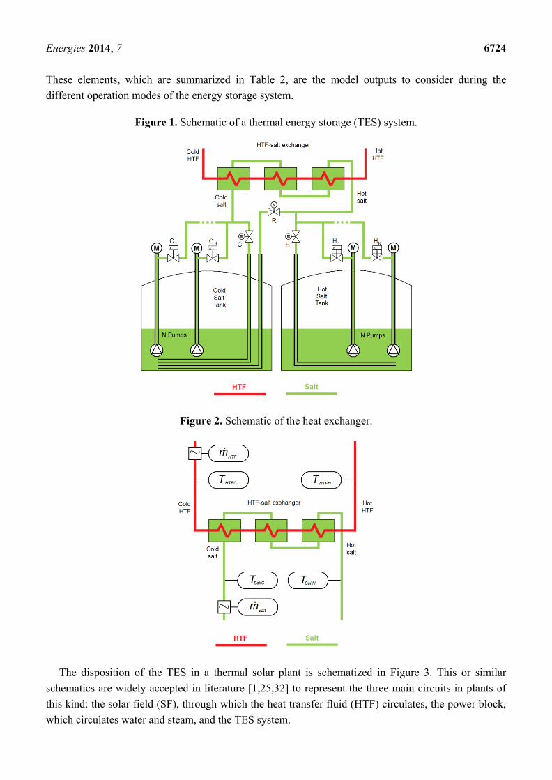
Conventional systems consist of: one cold salt tank, one hot salt tank, an HTF-salt exchanger, pumps

(to move the molten salt from one tank into the other), pipes and control valves. Figure 1 shows a

typical schematic that includes a single train formed by three exchangers and Table 1 shows the

control elements (and their respective control variables) identified in this schematic; flow directions in

this schematic depend on whether the heat storage system is being charged (HTF flows from the hot

side to the cold side, salt flows from the cold tank to the hot tank) or discharged. The model to develop

must include the set points of the control variables as inputs, since the state of the elements they

control will determine the performance of the TES.

Similarly, the model must have several outputs that allow users checking whether the response of

the system is the expected one or not. Process outputs are monitored in actual systems by means of

several sensors placed at the inputs and outputs of the heat exchanger as shown in Figure 2.

Energies 2014, 7 6724

These elements, which are summarized in Table 2, are the model outputs to consider during the

different operation modes of the energy storage system.

Figure 1. Schematic of a thermal energy storage (TES) system.

Figure 2. Schematic of the heat exchanger.

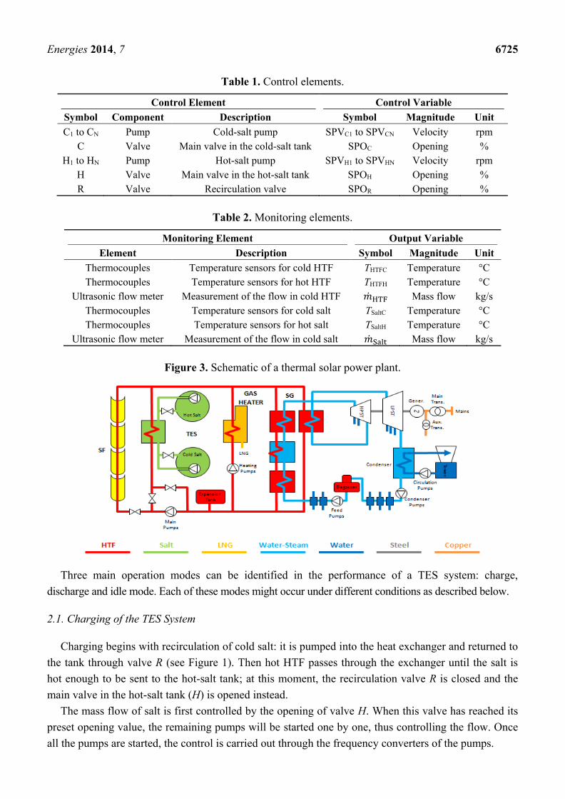
The disposition of the TES in a thermal solar plant is schematized in Figure 3. This or similar

schematics are widely accepted in literature [1,25,32] to represent the three main circuits in plants of

this kind: the solar field (SF), through which the heat transfer fluid (HTF) circulates, the power block,

which circulates water and steam, and the TES system.

Energies 2014, 7 6725

Table 1. Control elements.

Control Element Control Variable

Symbol Component Description Symbol Magnitude Unit

C1 to CN Pump Cold-salt pump SPVC1 to SPVCN Velocity rpm

C Valve Main valve in the cold-salt tank SPOC Opening %

H1 to HN Pump Hot-salt pump SPVH1 to SPVHN Velocity rpm

H Valve Main valve in the hot-salt tank SPOH Opening %

R Valve Recirculation valve SPOR Opening %

Table 2. Monitoring elements.

Monitoring Element Output Variable

Element Description Symbol Magnitude Unit

Thermocouples Temperature sensors for cold HTF THTFC Temperature °C

Thermocouples Temperature sensors for hot HTF THTFH Temperature °C

Ultrasonic flow meter Measurement of the flow in cold HTF ��HTF Mass flow kg/s

Thermocouples Temperature sensors for cold salt TSaltC Temperature °C

Thermocouples Temperature sensors for hot salt TSaltH Temperature °C

Ultrasonic flow meter Measurement of the flow in cold salt ��Salt Mass flow kg/s

Figure 3. Schematic of a thermal solar power plant.

Three main operation modes can be identified in the performance of a TES system: charge,

discharge and idle mode. Each of these modes might occur under different conditions as described below.

2.1. Charging of the TES System

Charging begins with recirculation of cold salt: it is pumped into the heat exchanger and returned to

the tank through valve R (see Figure 1). Then hot HTF passes through the exchanger until the salt is

hot enough to be sent to the hot-salt tank; at this moment, the recirculation valve R is closed and the

main valve in the hot-salt tank (H) is opened instead.

The mass flow of salt is first controlled by the opening of valve H. When this valve has reached its

preset opening value, the remaining pumps will be started one by one, thus controlling the flow. Once

all the pumps are started, the control is carried out through the frequency converters of the pumps.

Energies 2014, 7 6726

Tables 3–5 include all the variables involved in the process described above are: input variables

(used to control the elements included in Table 1), perturbation variables affecting the process and

output variables (quantifiable by means of the monitoring elements indicated in Table 2).

Table 3. TES charging input variables.

Charging of the TES System

Input Variable Description

SPVCi Set Point for the speed defined by the frequency converter of the i-th cold-salt pump

SPOH Set Point for the opening of the main valve in the hot-salt tank

SPOR Set Point for the opening of the recirculation valve

Table 4. TES charging perturbations.

Charging of the TES System

Perturbation Perturbation

THTFH Hot HTF temperature at the input of the heat exchanger

TSaltC Cold salt temperature at the input of the heat exchanger

��HTF HTF mass flow through the heat exchanger

Table 5. TES charging output variables.

Charging of the TES System

Output Variable Description

THTFC Cold HTF temperature at the output of the heat exchanger

TSaltH Hot salt temperature at the output of the heat exchanger (control variable)

��Salt Molten salt mass flow through the heat exchanger

The goal during this operation mode is regulating temperature TSaltH by adequately setting the values

of SPVCi, SPOH and SPOR while taking perturbations into account and having the other output

variables provide insight into what is actually happening. The model to develop must make all these

variables available. Figure 4 shows a block representation of the charging process.

Figure 4. Process block associated to TES charging.

Energies 2014, 7 6727

It must be noticed that, depending on whether it is the solar field (SF) or the gas heater that supplies

the thermal energy storage (TES) system (and perhaps the steam generator system, SGS, as well),

charging of the thermal energy storage system can take place in either of the following ways.

2.1.1. From SF to SGS + TES

In some summer days, around noon, the thermal energy produced by the solar field (SF) is greater

than that required to operate the turbine at nominal power. This excess of energy must be stored in the

molten salt while the steam generation system (SGS) keeps operating at nominal power.

2.1.2. From SF to TES

In winter days, when the thermal power provided by the solar field is not enough to operate the

turbine with an acceptable efficiency, the choice is storing all of this energy in the molten salt.

2.1.3. From Gas Heater to TES

When the molten salt needs to be heated but there is not enough energy coming from the solar field,

the gas heater can be used for this purpose.

The difficulty associated to the control of each of these charging processes varies according to the

variations of HTF mass flow and temperature during the charge.

2.2. Discharging of the TES System

Discharge begins by pumping hot salt through the heat exchanger and into the cold-salt tank

through its main valve (C). Then cold HTF passes through the exchanger to be heated. As HTF flow

increases, salt flow is increased too by opening valve C. When this valve has reached its preset

opening value, the remaining pumps will be started one by one, thus controlling the flow. Once all the

pumps are started, the control is carried out through the frequency converters of the pumps.

The variables involved in the process described above are summarized in Tables 6 to 8:

Table 6. TES discharging input variables.

Discharging of the TES System

Input Var. Description

SPVHi Set Point for the speed defined by the frequency converter of the i-th hot-salt pump

SPOC Set Point for the opening of the main valve in the cold-salt tank

Table 7. TES discharging perturbations.

Discharging of the TES System

Perturbation Description

THTFC Cold HTF temperature at the input of the heat exchanger

TSaltH Hot salt temperature at the input of the heat exchanger

��HTF HTF mass flow through the heat exchanger

Energies 2014, 7 6728

Table 8. TES discharging output variables.

Discharging of the TES System

Output Var. Description

THTFH Hot HTF temperature at the output of the heat exchanger (control variable)

TSaltC Cold salt temperature at the output of the heat exchanger

��Salt Molten salt mass flow through the heat exchanger

The goal in this case is regulating temperature THTFH by adequately setting the values of SPVHi and

SPOC while taking perturbations into account and having the other output variables provide insight

into what is actually happening. A possible block representation of the discharging process that

presents all the variables described above is shown in Figure 5.

Figure 5. Process block associated to TES discharging.

Similarly to the charging process, discharging the thermal energy storage system can also take place

in either of the following ways.

2.2.1. From SF + TES to SGS

The energy provided by the solar field is not enough to have the steam generation system provide

the power required. The thermal energy storage system supplies additional energy to make the SGS

operate as close as possible to nominal power conditions.

2.2.2. From TES to SGS

All the energy provided by the generator comes from the TES (typical situation at nights). The

power obtained is slightly lower than nominal power.

2.2.3. From TES + Gas Heater to SGS.

Sometimes the TES system cannot provide enough energy to operate the steam generation system at

the required power. In these cases, the gas heater can be used to supply additional energy.

Energies 2014, 7 6729

Regulation of both the charge and discharge processes experiences several problems, namely:

process perturbations, measurement errors and non-linearity. As already stated, optimization of all

these processes cannot be carried out unless an accurate model of the process is available.

2.3. TES System in Idle Mode

This mode corresponds to the idle times between charge and discharge. No regulation is required

during this mode.

After the TES system has been fully charged, it enters idle mode, with the hot-salt tank full, until

the SF cannot keep the turbine operating at nominal power.

After the TES has been completely discharged, it enters idle mode, with the hot-salt tank empty,

until the SF provides an excess of thermal power above that required by the turbines (typically the

following day).

3. Model Definition

Up to this point, two models have been described: one for the charge and another for the discharge

of the TES system. It might be argued that having two process models is not functional since the

system is the same in both cases. Despite this being true, the fact that internal flows are opposite

during charge and discharge, and that relevant input/output variables change for each case, has led

authors to consider it more convenient to have two separate models. In addition, charge and discharge

are completely independent process (either the TES system is charging or it is discharging) and can

therefore be optimized separately.

Whatever the model considered (charge or discharge), only three basic equations are needed to

define the performance of a thermal energy storage system: mass conservation, energy conservation

and heat transmission. Other than that, the models must accurately define the mass flows within

the system.

The rest of the paper focuses on the description of a model associated to the charge process of a

TES to be included in a simulation oriented visual environment. Although Matlab-Simulink blocks are

shown, any other simulation environment of these characteristics could be used. The model will be

developed by carrying out a top-down partitioning of the system in order to have it implemented

bottom-up later. The model associated to the discharge can be similarly obtained.

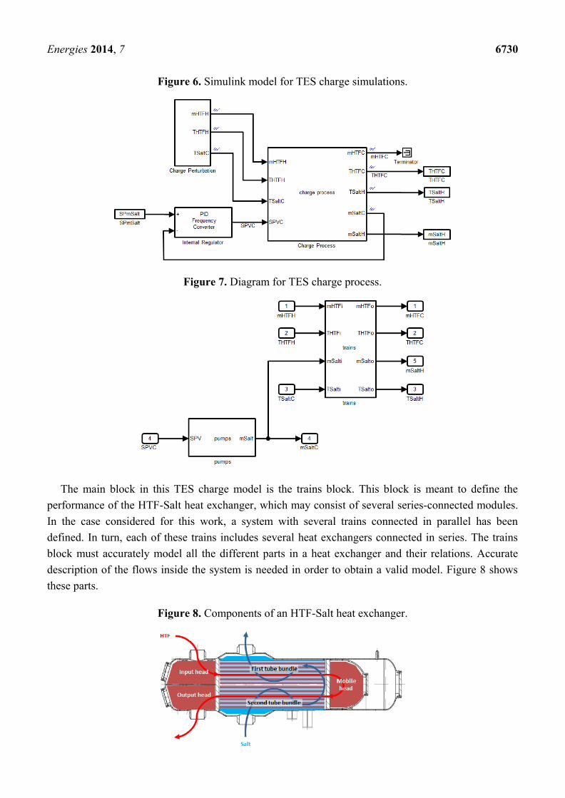
Figure 6 shows the simplified model associated to the charge process in the TES system. As can be

seen, the set points of the valves are not directly provided in actual systems. Instead, there is a simple

internal PID regulator that implements mass-flow control through the frequency converters of the

pumps. This is represented in the figure and considered to be part of the model to be derived.

From this point on, the aforementioned top-down analysis is carried out so that the subsystems

included in each block are defined. To start with, the TES charge process is modeled by the pumps

controlling the mass flow entering the trains of exchangers as indicated in Figure 7. The TES discharge

model will only differ from this in the input and output variables (refer to Figure 5 to see

these variables).

Energies 2014, 7 6730

Figure 6. Simulink model for TES charge simulations.

Figure 7. Diagram for TES charge process.

The main block in this TES charge model is the trains block. This block is meant to define the

performance of the HTF-Salt heat exchanger, which may consist of several series-connected modules.

In the case considered for this work, a system with several trains connected in parallel has been

defined. In turn, each of these trains includes several heat exchangers connected in series. The trains

block must accurately model all the different parts in a heat exchanger and their relations. Accurate

description of the flows inside the system is needed in order to obtain a valid model. Figure 8 shows

these parts.

Figure 8. Components of an HTF-Salt heat exchanger.

Energies 2014, 7 6731

Shell-and-tube heat exchangers are very common in process industry and their transient modeling

has been subject of numerous publications [33–35]. Accurate modeling of this kind of devices involves

considering the shell-side convective heat transfer over the tube bundle in detail. This is typically done

via the Bell-Delaware method [36–38], which is an empirical method based on numerous experiments

with shell-and-tube heat exchangers. Recently, there have also been published some numerical studies

that reconfirmed its validity [39–41].

However, the model of the thermal energy storage system does not require a very accurate

heat-exchanger model to adequately define the heat transfer. The heat exchanger model should

accurately represent the dynamic effects that provide the TES model with a good estimation of the

time-evolution of the system operations. Different heat transfer models for the heat-exchangers have

been tried by the authors with negligible impact on the simulation results, and with complex heat

transfer models increasing the computational time due to the complexity of the overall model. In

addition, 2-D or 3-D models have been tried for the heat exchangers sections or volumes, with

negligible impact on the simulation results. In fact, experience has shown that, rather than a high

accuracy in temperature values, it is necessary to have a system that adequately models the delays

produced in very large heat exchangers like the ones used in these power plants. It must be taken into

account that these heat exchangers might consist of up to six trains connected in series (as is the case in

Andasol I, a 150-MW thermal power plant in Andalusia, southern Spain), which results in relatively

long delays before the response is obtained at the output. Should these delays not be properly modeled,

the parameters of the PID regulator that controls the overall system cannot be adequately calculated,

thus giving rise to abnormal operation.

Thus, a simple 1-D model has been used to define the heat exchanger. The flux exchange is

considered to be unidirectional and the bundles are divided into smaller discrete parts where the basic

heat transfer equations will be solved. No 3-D simulation of the shell is deemed necessary.

The interface variables for the heat exchanger are shown in Tables 9 and 10.

Table 9. Heat exchanger input variables.

Heat Exchanger

Input Var. Description

��HTFi Input HTF mass flow

THTFi Input HTF temperature

THTFc Counterflow input HTF temperature

��Salti Input salt mass flow

TSalti Input salt temperature

TSaltc Counterflow input salt temperature

Table 10. Heat exchanger output variables.

Discharging of the TES System

Output Var. Description

��HTFo Output HTF mass flow

THTFo Output HTF temperature

��Salto Output salt mass flow

TSalto Output salt temperature

Energies 2014, 7 6732

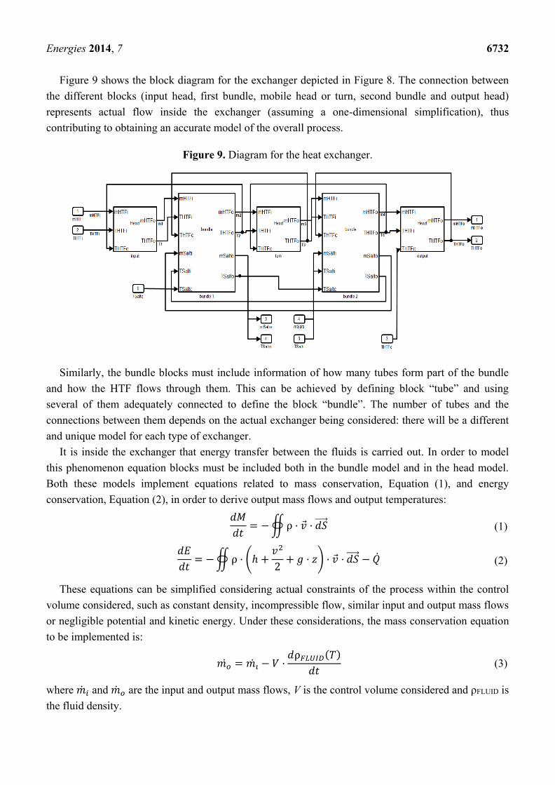
Figure 9 shows the block diagram for the exchanger depicted in Figure 8. The connection between

the different blocks (input head, first bundle, mobile head or turn, second bundle and output head)

represents actual flow inside the exchanger (assuming a one-dimensional simplification), thus

contributing to obtaining an accurate model of the overall process.

Figure 9. Diagram for the heat exchanger.

Similarly, the bundle blocks must include information of how many tubes form part of the bundle

and how the HTF flows through them. This can be achieved by defining block “tube” and using

several of them adequately connected to define the block “bundle”. The number of tubes and the

connections between them depends on the actual exchanger being considered: there will be a different

and unique model for each type of exchanger.

It is inside the exchanger that energy transfer between the fluids is carried out. In order to model

this phenomenon equation blocks must be included both in the bundle model and in the head model.

Both these models implement equations related to mass conservation, Equation (1), and energy

conservation, Equation (2), in order to derive output mass flows and output temperatures:

𝑑𝑀

𝑑𝑡= − ∯ ρ · �� · 𝑑𝑆 (1)

𝑑𝐸

𝑑𝑡= − ∯ ρ · (ℎ +

𝑣2

2+ 𝑔 · 𝑧) · �� · 𝑑𝑆 − �� (2)

These equations can be simplified considering actual constraints of the process within the control

volume considered, such as constant density, incompressible flow, similar input and output mass flows

or negligible potential and kinetic energy. Under these considerations, the mass conservation equation

to be implemented is:

𝑚𝑜 = 𝑚𝑖 − 𝑉 ·𝑑ρ𝐹𝐿𝑈𝐼𝐷(𝑇)

𝑑𝑡 (3)

where ��𝑖 and ��𝑜 are the input and output mass flows, V is the control volume considered and ρFLUID is

the fluid density.

Energies 2014, 7 6733

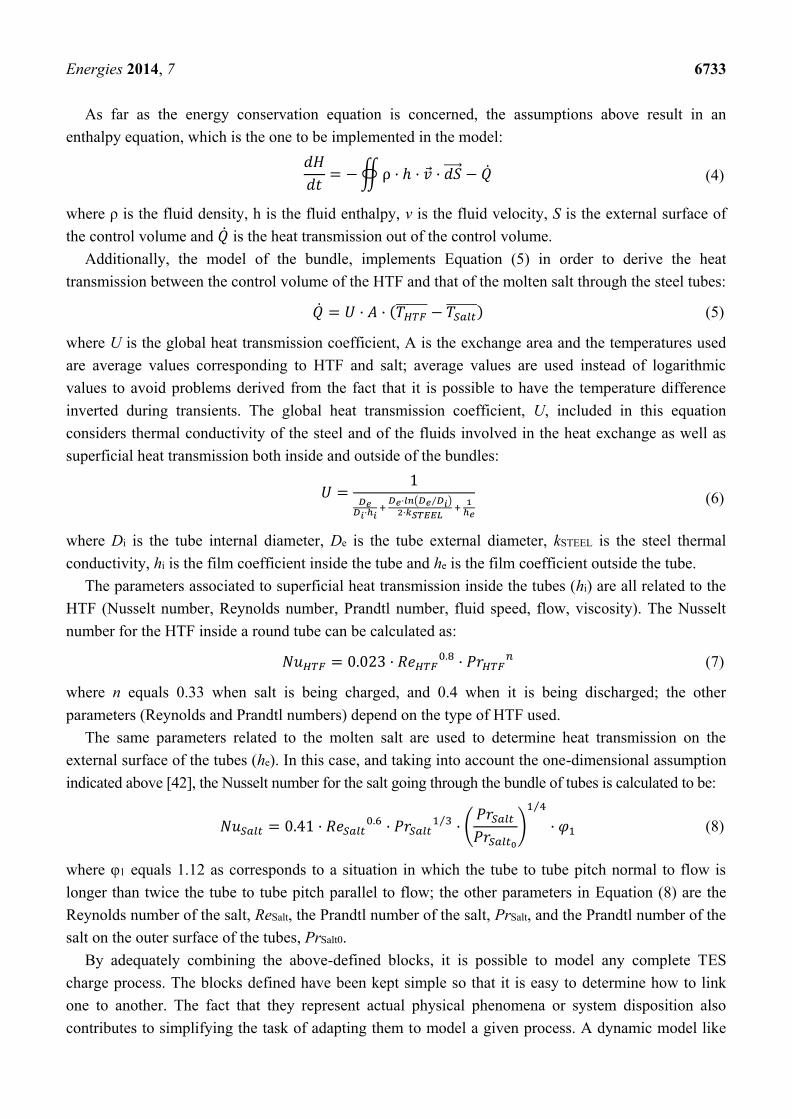
As far as the energy conservation equation is concerned, the assumptions above result in an

enthalpy equation, which is the one to be implemented in the model:

𝑑𝐻

𝑑𝑡= − ∯ ρ · ℎ · �� · 𝑑𝑆 − �� (4)

where ρ is the fluid density, h is the fluid enthalpy, v is the fluid velocity, S is the external surface of

the control volume and �� is the heat transmission out of the control volume.

Additionally, the model of the bundle, implements Equation (5) in order to derive the heat

transmission between the control volume of the HTF and that of the molten salt through the steel tubes:

�� = 𝑈 · 𝐴 · (𝑇𝐻𝑇𝐹 − 𝑇𝑆𝑎𝑙𝑡

) (5)

where U is the global heat transmission coefficient, A is the exchange area and the temperatures used

are average values corresponding to HTF and salt; average values are used instead of logarithmic

values to avoid problems derived from the fact that it is possible to have the temperature difference

inverted during transients. The global heat transmission coefficient, U, included in this equation

considers thermal conductivity of the steel and of the fluids involved in the heat exchange as well as

superficial heat transmission both inside and outside of the bundles:

𝑈 =1

𝐷𝑒𝐷𝑖·ℎ𝑖

+ 𝐷𝑒·𝑙𝑛(𝐷𝑒 𝐷𝑖⁄ )

2·𝑘𝑆𝑇𝐸𝐸𝐿 +

1ℎ𝑒

(6)

where Di is the tube internal diameter, De is the tube external diameter, kSTEEL is the steel thermal

conductivity, hi is the film coefficient inside the tube and he is the film coefficient outside the tube.

The parameters associated to superficial heat transmission inside the tubes (hi) are all related to the

HTF (Nusselt number, Reynolds number, Prandtl number, fluid speed, flow, viscosity). The Nusselt

number for the HTF inside a round tube can be calculated as:

𝑁𝑢𝐻𝑇𝐹 = 0.023 · 𝑅𝑒𝐻𝑇𝐹0.8 · 𝑃𝑟𝐻𝑇𝐹

𝑛 (7)

where n equals 0.33 when salt is being charged, and 0.4 when it is being discharged; the other

parameters (Reynolds and Prandtl numbers) depend on the type of HTF used.

The same parameters related to the molten salt are used to determine heat transmission on the

external surface of the tubes (he). In this case, and taking into account the one-dimensional assumption

indicated above [42], the Nusselt number for the salt going through the bundle of tubes is calculated to be:

𝑁𝑢𝑆𝑎𝑙𝑡 = 0.41 · 𝑅𝑒𝑆𝑎𝑙𝑡0.6 · 𝑃𝑟𝑆𝑎𝑙𝑡

1 3⁄ · (𝑃𝑟𝑆𝑎𝑙𝑡

𝑃𝑟𝑆𝑎𝑙𝑡0

)

1 4⁄

· 𝜑1 (8)

where φ1 equals 1.12 as corresponds to a situation in which the tube to tube pitch normal to flow is

longer than twice the tube to tube pitch parallel to flow; the other parameters in Equation (8) are the

Reynolds number of the salt, ReSalt, the Prandtl number of the salt, PrSalt, and the Prandtl number of the

salt on the outer surface of the tubes, PrSalt0.

By adequately combining the above-defined blocks, it is possible to model any complete TES

charge process. The blocks defined have been kept simple so that it is easy to determine how to link

one to another. The fact that they represent actual physical phenomena or system disposition also

contributes to simplifying the task of adapting them to model a given process. A dynamic model like

Energies 2014, 7 6734

the one presented here is necessary in order to optimize the TES process as a whole, especially its

regulation. Nowadays, the control of this process is performed by means of simple, non-optimized

control methods. The model presented in this paper might contribute to improving the state of the art

by allowing advanced control techniques to be tested so that more convenient algorithms can be

implemented in this part of the power plant and, hence, improve the overall performance of the plant.

4. Model Validation

Validation of the model presented was carried out in two stages. Firstly, simple simulations were

run in order to find out whether the results obtained were consistent with the behavior expected.

Secondly, the information provided by the model was compared to that measured in an actual plant.

Two simulations were run considering the two most usual control strategies to regulate this kind of

processes: a so-called semiautomatic control and a PID regulator. These control methods are very

popular and widely used for TES regulation. Since they are well-known strategies, they will be used

together with the model developed in order to validate its performance. The main features of these

control methods are sketched below.

In the case of semiautomatic control, an operator is in charge of observing the values of the output

variables and defining new set points for the input variables. Thus, the regulation will be carried out by

means of steps, the accuracy of which depends only on the operator’s experience. For a charge process,

this person will define the set point for the salt mass flow (SP��Salt) while observing the evolution of

the output salt temperature (TSaltH). Internal PID regulators will be in charge of operating the pumps so

that the set point fixed by the operator is achieved. Figure 10 shows a block diagram of the whole system.

Figure 10. Semiautomatic control of a TES charge process.

In a PID control, the person in charge is substituted by an external regulation loop. A simple PID

regulator is usually enough in these cases, and only the set point for the desired output salt temperature

must be provided. This system is depicted in Figure 11.

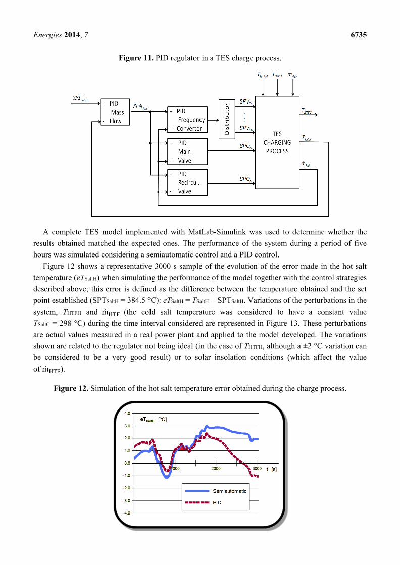
Energies 2014, 7 6735

Figure 11. PID regulator in a TES charge process.

A complete TES model implemented with MatLab-Simulink was used to determine whether the

results obtained matched the expected ones. The performance of the system during a period of five

hours was simulated considering a semiautomatic control and a PID control.

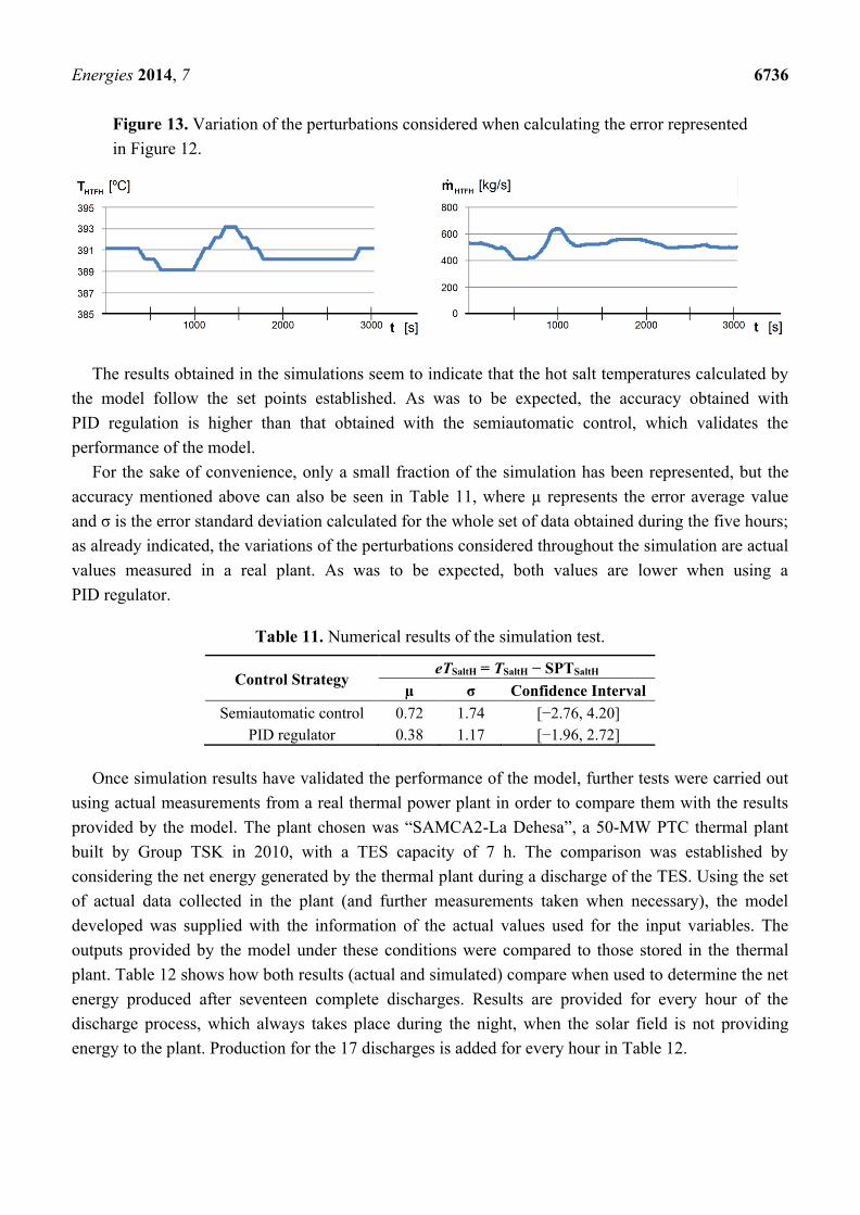
Figure 12 shows a representative 3000 s sample of the evolution of the error made in the hot salt

temperature (eTSaltH) when simulating the performance of the model together with the control strategies

described above; this error is defined as the difference between the temperature obtained and the set

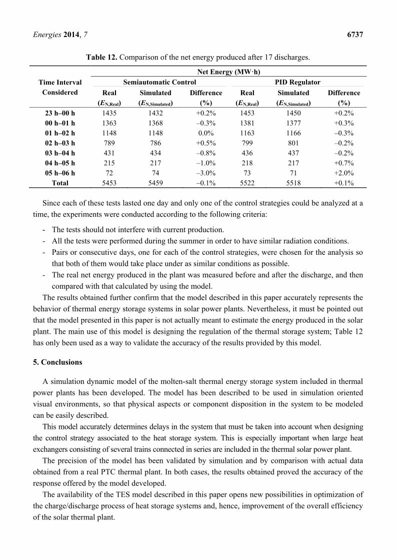
point established (SPTSaltH = 384.5 °C): eTSaltH = TSaltH − SPTSaltH. Variations of the perturbations in the

system, THTFH and mHTF (the cold salt temperature was considered to have a constant value

TSaltC = 298 °C) during the time interval considered are represented in Figure 13. These perturbations

are actual values measured in a real power plant and applied to the model developed. The variations

shown are related to the regulator not being ideal (in the case of THTFH, although a ±2 °C variation can

be considered to be a very good result) or to solar insolation conditions (which affect the value

of mHTF).

Figure 12. Simulation of the hot salt temperature error obtained during the charge process.

Energies 2014, 7 6736

Figure 13. Variation of the perturbations considered when calculating the error represented

in Figure 12.

The results obtained in the simulations seem to indicate that the hot salt temperatures calculated by

the model follow the set points established. As was to be expected, the accuracy obtained with

PID regulation is higher than that obtained with the semiautomatic control, which validates the

performance of the model.

For the sake of convenience, only a small fraction of the simulation has been represented, but the

accuracy mentioned above can also be seen in Table 11, where µ represents the error average value

and σ is the error standard deviation calculated for the whole set of data obtained during the five hours;

as already indicated, the variations of the perturbations considered throughout the simulation are actual

values measured in a real plant. As was to be expected, both values are lower when using a

PID regulator.

Table 11. Numerical results of the simulation test.

Control Strategy eTSaltH = TSaltH − SPTSaltH

µ σ Confidence Interval

Semiautomatic control 0.72 1.74 [−2.76, 4.20]

PID regulator 0.38 1.17 [−1.96, 2.72]

Once simulation results have validated the performance of the model, further tests were carried out

using actual measurements from a real thermal power plant in order to compare them with the results

provided by the model. The plant chosen was “SAMCA2-La Dehesa”, a 50-MW PTC thermal plant

built by Group TSK in 2010, with a TES capacity of 7 h. The comparison was established by

considering the net energy generated by the thermal plant during a discharge of the TES. Using the set

of actual data collected in the plant (and further measurements taken when necessary), the model

developed was supplied with the information of the actual values used for the input variables. The

outputs provided by the model under these conditions were compared to those stored in the thermal

plant. Table 12 shows how both results (actual and simulated) compare when used to determine the net

energy produced after seventeen complete discharges. Results are provided for every hour of the

discharge process, which always takes place during the night, when the solar field is not providing

energy to the plant. Production for the 17 discharges is added for every hour in Table 12.

Energies 2014, 7 6737

Table 12. Comparison of the net energy produced after 17 discharges.

Time Interval

Considered

Net Energy (MW·h)

Semiautomatic Control PID Regulator

Real

(EN,Real)

Simulated

(EN,Simulated)

Difference

(%)

Real

(EN,Real)

Simulated

(EN,Simulated)

Difference

(%)

23 h–00 h 1435 1432 +0.2% 1453 1450 +0.2%

00 h–01 h 1363 1368 –0.3% 1381 1377 +0.3%

01 h–02 h 1148 1148 0.0% 1163 1166 –0.3%

02 h–03 h 789 786 +0.5% 799 801 –0.2%

03 h–04 h 431 434 –0.8% 436 437 –0.2%

04 h–05 h 215 217 –1.0% 218 217 +0.7%

05 h–06 h 72 74 –3.0% 73 71 +2.0%

Total 5453 5459 –0.1% 5522 5518 +0.1%

Since each of these tests lasted one day and only one of the control strategies could be analyzed at a

time, the experiments were conducted according to the following criteria:

- The tests should not interfere with current production.

- All the tests were performed during the summer in order to have similar radiation conditions.

- Pairs or consecutive days, one for each of the control strategies, were chosen for the analysis so

that both of them would take place under as similar conditions as possible.

- The real net energy produced in the plant was measured before and after the discharge, and then

compared with that calculated by using the model.

The results obtained further confirm that the model described in this paper accurately represents the

behavior of thermal energy storage systems in solar power plants. Nevertheless, it must be pointed out

that the model presented in this paper is not actually meant to estimate the energy produced in the solar

plant. The main use of this model is designing the regulation of the thermal storage system; Table 12

has only been used as a way to validate the accuracy of the results provided by this model.

5. Conclusions

A simulation dynamic model of the molten-salt thermal energy storage system included in thermal

power plants has been developed. The model has been described to be used in simulation oriented

visual environments, so that physical aspects or component disposition in the system to be modeled

can be easily described.

This model accurately determines delays in the system that must be taken into account when designing

the control strategy associated to the heat storage system. This is especially important when large heat

exchangers consisting of several trains connected in series are included in the thermal solar power plant.

The precision of the model has been validated by simulation and by comparison with actual data

obtained from a real PTC thermal plant. In both cases, the results obtained proved the accuracy of the

response offered by the model developed.

The availability of the TES model described in this paper opens new possibilities in optimization of

the charge/discharge process of heat storage systems and, hence, improvement of the overall efficiency

of the solar thermal plant.

Energies 2014, 7 6738

Author Contributions

This paper is part of the PhD Thesis developed by Rogelio Peón Menéndez, who has therefore

carried out most of the work presented here. Professors Juan Á. Martínez and Miguel J. Prieto were the

supervisors of this work, whereas Lourdes Á. Barcia and Juan M. Martín Sánchez respectively assisted

Rogelio Peón with Simulink simulations and regulation topics.

Conflicts of Interest

The authors declare no conflict of interest.

References

1. Yang, Z.; Garimella, S.V. Cyclic operation of molten-salt thermal energy storage in thermoclines

for solar power plants. Appl. Energy 2013, 103, 256–265.

2. Usaola, J. Operation of concentrating solar power plants with storage in spot electricity markets.

IET Renew. Power Gener. 2012, 6, 59–66.

3. Weinrabe, G.; Ortmanns, W. Solar thermal power plants. In Renewable Energy; Kaltschmitt, M.,

Streicher, W., Wiese, A., Eds.; Springer: Berlin, Germany, 2007; pp. 171–228.

4. Schnatbaum, L. Solar thermal power plants. Eur. Phys. J. Spec. Top. 2009, 176, 127–140.

5. Wu, S.Y.; Xiao, L.; Cao, Y.; Li, Y.R. A parabolic dish/AMTEC solar thermal power system and

its performance evaluation. Appl. Energy 2010, 87, 452–462.

6. Ter-Gazarian, A.G. Thermal Energy Storage. In Energy Storage for Power Systems; IET Press:

Stevenage, UK, 2011; pp. 55–76.

7. Sangster, A.J. Intermittency buffers. In Green Energy and Technology. Energy for a Warming

World; Sangster, A.J., Ed.; Springer: Berlin, Germany, 2010; pp. 81–123.

8. Steinmann, W.D.; Laing, D.; Tamme, R. Storage systems for solar steam. In Proceedings of ISES

World Congress 2007 (Vol. I – Vol. V); Springer: Berlin, Germany, 2007; pp. 2736–2740.

9. Laing, D.; Steinmann, W.D.; Tamme, R. Sensible heat storage for medium and high temperatures.

In Proceedings of ISES World Congress 2007 (Vol. I – Vol. V); Springer: Berlin, Germany, 2007;

pp. 2731–2735.

10. Goods, S.H.; Bradshaw, R.W. Corrosion of stainless steels and carbon steel by molten mixtures of

commercial nitrate salts. J. Mater. Eng. Perform. 2004, 13, 78–87.

11. USA Trough Initiative. Thermal Storage Oil-to-Salt Heat Exchanger Design and Safety Analysis;

Task Order Au. No. KAF-9-29765-09; Nexant Inc.: San Francisco, CA, USA, 2000.

12. Annaratone, D. Engineering Heat Transfer; Springer: Berlin, Germany, 2010.

13. Massoud, M. Engineering Thermofluids; Springer: Berlin, Germany, 2005.

14. Damsker, D.J.; Sandberg, C. Towards advanced concurrency, distribution, integration, and

openness of a power plant distributed control system (DCS). IEEE Trans. Energy Convers. 1991,

6, 297–302.

15. Bong-Kuk, L.; Yong-Hak, S. The integrated monitoring and control system for the combined

cycle power plant. In Proceedings of the International Conference on Control, Automation and

Systems, Seoul, Korea, 14–17 October 2008; pp. 1479–1483.

Energies 2014, 7 6739

16. Rajasekaran, S. A Simplified predictive control for a shell and tube heat exchanger. Int. J.

Eng. Sci. 2010, 2, 7245–7251.

17. Garcia, C.E.; Prett, D.M. Model predictive control: Theory and practice—A survey. Automatica

1989, 25, 335–348.

18. Lim, K.W.; Ling, K.V. Generalized predictive control of a heat exchanger. IEEE Control

Syst. Mag. 1989, 1, 9–12.

19. Nelles, O. Nonlinear System Identification: From Classical Approaches to Neural Networks and

Fuzzy Models; Springer: Berlin, Germany, 2001.

20. Imal, E. CDM based controller design for nonlinear heat exchanger process. Turk. J. Electr. Eng.

Comput. Sci. 2009, 17, 143–161.

21. Skrjanc, I.; Matko, D. Predictive functional control based on fuzzy model for heat-exchanger pilot

plant. IEEE Trans. Fuzzy Syst. 2000, 8, 705–712.

22. Hooshang Mazinan, A.; Sadati, N. Fuzzy predictive control based multiple models strategy for a

tubular heat exchanger system. Appl. Intell. 2010, 33, 247–263.

23. Badgwell, A.B.; Qin, S.J.; Kouvaritakis, B. Review of nonlinear model predictive control

applications. IEE Control Ser. 2001, 3, 3–32.

24. Parker, R.S.; Gatzke, E.P.; Mahadevan, R.; Meadows, E.S.; Kouvaritakis, F.J.; Doyle, B.

Nonlinear model predictive control: Issues and applications. IEE Control Ser. 2001, 5, 34–57.

25. Llorente García, I.; Álvarez, J.L.; Blanco, D. Performance model for parabolic trough solar

thermal power plants with thermal storage: Comparison to operating plant data. Sol. Energy 2011,

85, 2443–2460.

26. Niknia, I.; Yaghoubi, M. Transient simulation for developing a combined solar thermal power plant.

Appl. Therm. Eng. 2012, 37, 196–207.

27. Rolim, M.M.; Fraidenraich, N.; Tiba, C. Analytic modeling of a solar power plant with parabolic

linear collectors. Sol. Energy 2009, 83, 126–133.

28. Powell, K.M.; Hedengren, J.D.; Edgar, T.F. Dynamic optimization of a solar thermal energy

storage system over a 24 h period using weather forecasts. In Proceedings of the American

Control Conference, Washington, DC, USA, 17–19 June 2013; pp. 2946–2951.

29. Powell, K.M.; Edgar, T.F. Modeling and control of a solar thermal power plant with thermal

energy storage. Chem. Eng. Sci. 2012, 71, 138–145.

30. Kibaara, S.; Chowdhury, S.; Chowdhury, S.P. Analysis of Cooling Methods of Parabolic Trough

Concentrating Solar Thermal Power Plant. In Proceedings of the 2012 IEEE International

Conference on Power System Technology, Auckland, New Zealand, 30 October–2 November

2012; pp. 1–6.

31. Solar Advisor Model. Available online: https://sam.nrel.gov (accessed on 24 July 2014).

32. Martín, L.; Zarzalejo, L.F.; Polo, J.; Navarro, A.; Marchante, R.; Cony, M. Prediction of global

solar irradiance based on time series analysis: Application to solar thermal power plants energy

production planning. Sol. Energy 2012, 84, 1772–1781.

33. Fraser, K.F.; Hollands, K.G.T.; Brunger, P. An empirical model for natural convection heat

exchangers in SDHW systems. Sol. Energy 1995, 55, 75–84.

Energies 2014, 7 6740

34. Vera-García, F.; García-Cascales, J.R.; Gonzálvez-Maciá, J.; Cabello, R.; Llopis, R.; Sanchez, D.;

Torrella, E. A simplified model for shell-and-tubes heat exchangers: Practical application.

Appl. Therm. Eng. 2010, 30, 1231–1241.

35. Ravagnani, M.A.S.S.; Caballero, J.A. A MINLP model for the rigorous design of shell and tube

heat exchangers using the tema standards original. Chem. Eng. Res. Des. 2007, 85, 1423–1435.

36. Green, D.W.; Perry, R.H. Perry’s Chemical Engineer’s Handbook, 6th ed.; McGraw-Hill:

New York, NY, USA, 1984; Sections 10–11.

37. Kakaç, S.; Liu, H. Heat Exchangers, Selection, Rating and Thermal Design; CRC Press:

Boca Raton, FL, USA, 1995; p. 53.

38. Peters, M.S.; Timmerhaus, K.; West, R.E. Plant Design and Economics for Chemical Engineers,

5th ed.; McGraw-Hill Professional: New York, NY, USA, 2003; pp. 716–724.

39. Tan, X.H.; Zhu, D.S.; Zhou, G.Y.; Yang, L. 3D numerical simulation on the shell side heat

transfer and pressure drop performances of twisted oval tube heat exchanger. Int. J. Heat

Mass Transf. 2013, 65, 244–253.

40. You, Y.; Fan, A.; Huang, S.; Liu, W. Numerical modeling and experimental validation of heat

transfer and flow resistance on the shell side of a shell-and-tube heat exchanger with flower baffles.

Int. J. Heat Mass Transf. 2012, 55, 7561–7569.

41. You, Y.; Fan, A.; Lai, X.; Huang, S.; Liu, W. Experimental and numerical investigations of

shell-side thermo-hydraulic performances for shell-and-tube heat exchanger with trefoil-hole baffles.

Appl. Therm. Eng. 2013, 50, 950–956.

42. Zukauskas, A. Heat transfer from tubes in crossflow. In Advances in Heat Transfer; Irvine, T.F., Jr.,

Hartnett, J.P., Eds.; Academic Press, Inc.: New York, NY, USA, 1987; Volume 18, pp. 87–159.

© 2014 by the authors; licensee MDPI, Basel, Switzerland. This article is an open access article

distributed under the terms and conditions of the Creative Commons Attribution license

(http://creativecommons.org/licenses/by/4.0/).