A NOVEL MULTIPURPOSE EXCEL TOOL FOR EQUILIBRIUM SPECIATION

Annali di Chimica, 96, 2006, by Società Chimica Italiana

(°), Corresponding Authors; E-mail: Fax: (++39)-0432-558803; e-mail: [email protected]; Fax: (++39)-0432-558803; e-mail: [email protected].

A NOVEL MULTIPURPOSE EXCEL TOOL FOR EQUILIBRIUM

SPECIATION BASED ON NEWTON-RAPHSON METHOD AND ON A

HYBRID GENETIC ALGORITHM

Silvia DEL PIERO, Andrea MELCHIOR, Pierluigi POLESE(°), Roberto PORTANOVA, Marilena TOLAZZI(°) Dipartimento di Scienze e Tecnologie Chimiche, Università di Udine, Via Cotonificio 108, I-33100 Udine, Italy Summary - A new algorithm for simulation of chemical equilibria is developed, based on classical Newton-Raphson method applied to mass balance. This tool, named EST (Equilibrium Speciation Tool), is improved by using a robust Genetic Algorithm. In addition, EST works by using Excel spreadsheets and therefore offers the innovation of a great simplicity and versatility. In fact, it allows the users to simulate, or to obtain from experimental data, desired chemical-physical parameters as well as to interact with other available or freely created Excel tools. The reliability of this utility is here proved by comparison with some published data by other authors, concerning both complicated homogeneous and heterogeneous equilibria. In addiction its flexibility is tested computing thermodynamic parameters by using experimental calorimetric data referred to the complex formation of cobalt(II) with a macrocyclic ligand. A brief review and comparison of the relative robustness and quickness of main numerical methods are also reported.

INTRODUCTION

The simulation of ionic and non-ionic speciation is of great importance in many fields: for example, bio-inorganic- chemists are interested in the speciation of fluids such as blood and urine, geo- and marine- chemists in studying the distribution of species in sea, estuarine, lake, river and ground water, whereas analytical- chemists often match with general speciation problems and need implementation of analytical methods. Also metallurgists are interested to study the distribution of species involved in corrosion and environmental chemists to the speciation of pollutants in aquatic systems. Speciation routines have therefore undergone great development and grown up as one of the core components of most computer programs devoted to the determination of solution equilibrium constants. In addition, more and more interest lies in obtaining simulated chemical-physical parameters, such as spectroscopic and thermodynamic quantities. In spite of the large availability of some excellent softwares devoted essentially to three main areas, i.e. chemical equilibria simulations,

1-9thermodynamical parameters determination,

10-21 geochemical

modelling,22-35

the need of flexible and easy to use tools is still present.

DEL PIERO and coworkers

For example, the Equilibria Package36 has been recently proposed, which provides various Java

Classes (an object-oriented language37) offering the additional opportunity to be used for solving

equilibria problems in a Web based interface. Unfortunately the Web browsers till now available is not able to provide the manipulating and graphing ability which are, on the other hand, typical of spreadsheet software. Even the recent version 3.0 of CHEMEQL

34, and JCHESS a graphical

interface for CHESS29 which are based on JAVA applets, works essentially as a traditional

programs. Some other developed applications

38-40 use spreadsheets or macro formulas present in one of the

most diffuse spreadsheet software such as Microsoft Excel, but they are generally limited to face specific, simple systems. On the other hand, we have no news of a more systematic approach to speciation by using Excel, with the exception of Equilibrium Expert. This is a Microsoft Excel Add-in for multiple equilibria simulations and parameter estimations

41, but is essentially devoted to

protein binding, thus not being so suitable to solve multicomponent/multiphase systems. In this contest a new application, working by using Microsoft Excel and named EST (Equilibrium Speciation Tool), is here presented together with a brief review of main aspects of simulation of chemical equilibria in solutions. EST is based on classical stoichiometric mass balance equations which allow the simulation of the free concentrations of the species involved in multiple equilibria: its great innovation consists in the flexibility of this software as the input and output data can be manipulated very freely by the users, taking advantage of the versatility of Excel. So people are allowed to build graphics but also to obtain chemical-physical parameters from both simulated and experimental data. Last but not least, EST is also able to interact with other available (Solver

34,42, SolverStat

43) or freely created Excel

tools depending on what the users require. The reliability of this utility is here tested by comparison with some published data by other authors, concerning both complicated homogeneous

44 and heterogeneous equilibria

45, its flexibility

by computing thermodynamic parameters using previous collected experimental calorimetric data46

referred to the complex formation of cobalt(II) with a macrocyclic ligand. The writing of EST, also stimulated a comparison with main numerical methods for the resolution of non linear equations systems, in order to evaluate their relative robustness and quickness: the detailed results are also reported.

SIMULATION METHODS

There are two general approaches to simulate complex equilibria systems: (i) Gibbs free-energy minimisation and (ii) equilibrium constant method. The former is based on the minimisation of the Gibbs energy of the considered system using stoichiometries based on explicit chemical reactions (stoichiometric algorithms) or approaches in which no explicit stoichiometric analysis of the system are used (nonstoichiometric algorithms)

8.

The nonstoichiometric methods are more suitable for multiphase complex systems and preferred in the geochemical, and chemical-engineering applications

47-49 as the resolution of large systems, even

in non standard conditions, is relatively easier. Approach (II) is more direct and used by most chemists which are familiar in dealing with ionic equilibria. It is based on the solution of a set of equilibrium conditions satisfying stoichiometric mass balance equations. To solve these equations various approaches are used

50, the most common being (a) Newton

Raphson (NR) resolution of the resulting nonlinear system of equations3,8,51

and (b) iterative resolution of one equation at time

1,4,6. Method (a) ensures a rapid quadratic convergence but requires

An Excel Tool for Equilibrium Speciation

3

initial estimates close enough to the true solution, (b) is generally slower. Both methods (a) and (b) can diverge in particular chemical systems. To bypass these inconveniences, a variety of tricks and procedures has been proposed in the course of the years and the research of new methods still continues. For example Mioshi and do Lago

52 proposed an algorithm based on extent of reaction instead of

mass balance. Brassard and Bodurtha53 studied various minimisation routines implemented in

MATLAB (Quasi-Newton, Gauss-Newton, Levemberg-Marquardt (LM), NR and the Nelder Mead Simplex) and proposed an algorithm based on LM method using a cubic polynomial line search and, in the small number of cases when convergence fails, a robust Simplex method. Colonna and D'Angola

54 have developed a stoichiometric algorithm based on a modified hierarchical approach in

which one reaction at time was solved. The authors checked it successfully on a single phase problem and claimed that it can be easily extended to multiphase equilibria. Other general or particular approaches to chemical equilibria have been also developed as a result of the great interest for new tools in this field

55-60.

EST MATHEMATICAL EQUILIBRIA EXPRESSIONS

In a solution elemental component and derived species can be individuated. At equilibrium, in a system with m components and n species, for a formation reaction the mass-action laws and mass-balance may be stated as follows: [ ]

1

ij

ma

j j ii

C Aβ=

= ∏ (1)

1

[ ]i

n

A i ij jj

T A a C=

= +∑ (2)

where i denotes a component and j a species; β

j is the formation constant of the j species, a

ij is the

stoichiometric coefficient of the component i in the species j, Cj is the concentration of a derived

species j, [Ai] the concentration of free component i and T

Ai is the total concentration of component

i. Equation (2) can rewritten as:

1

[ ] 0i

n

T i ij j Aij

f A a C T=

⎛ ⎞= + − =⎜ ⎟⎝ ⎠

∑ (3)

The terms in brackets represent the computed total concentration, while T

Ai is the analytical total

concentration. The equations coming from (2) individuate a nonlinear system of m equations with n unknown variables (the concentration of free components) that can be solved numerically. The mentioned treatment can be extended to different type of equilibria. In the case of Solubility Equilibrium it can be written: [ ]

1

ikm

a

k ii

Ksp A=

= ∏ (4)

where the index k denotes a partially soluble species and Ksp

k the correspondent Solubility Product

Constant. Then we can write:


[ ]1

0ik

ma

sp i kki

f A Ksp=

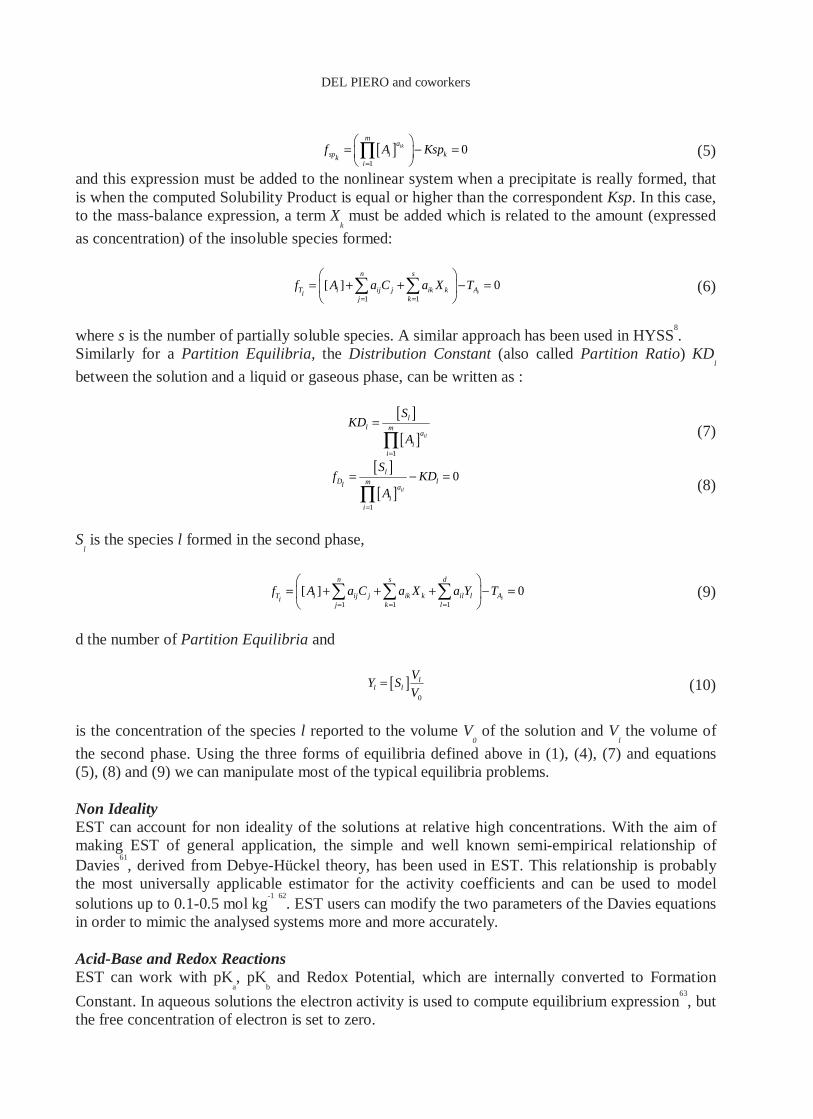
⎛ ⎞= − =⎜ ⎟⎝ ⎠∏ (5)

and this expression must be added to the nonlinear system when a precipitate is really formed, that is when the computed Solubility Product is equal or higher than the correspondent Ksp. In this case, to the mass-balance expression, a term X

k must be added which is related to the amount (expressed

as concentration) of the insoluble species formed:

1 1

[ ] 0i

n s

T i ij j ik k Aij k

f A a C a X T= =

⎛ ⎞= + + − =⎜ ⎟⎝ ⎠

∑ ∑ (6)

where s is the number of partially soluble species. A similar approach has been used in HYSS

8.

Similarly for a Partition Equilibria, the Distribution Constant (also called Partition Ratio) KDl

between the solution and a liquid or gaseous phase, can be written as : [ ]

[ ]1

il

ll m

a

ii

SKD

A=

=∏

(7)

[ ][ ]

1

0il

lD lml a

ii

Sf KD

A=

= − =∏

(8)

S

l is the species l formed in the second phase,

1 1 1

[ ] 0i

n s d

T i ij j ik k il l Aij k l

f A a C a X a Y T= = =

⎛ ⎞= + + + − =⎜ ⎟⎝ ⎠

∑ ∑ ∑ (9)

d the number of Partition Equilibria and [ ]

0

ll l

VY S

V= (10)

is the concentration of the species l reported to the volume V

0 of the solution and V

l the volume of

the second phase. Using the three forms of equilibria defined above in (1), (4), (7) and equations (5), (8) and (9) we can manipulate most of the typical equilibria problems. Non Ideality EST can account for non ideality of the solutions at relative high concentrations. With the aim of making EST of general application, the simple and well known semi-empirical relationship of Davies

61, derived from Debye-Hückel theory, has been used in EST. This relationship is probably

the most universally applicable estimator for the activity coefficients and can be used to model solutions up to 0.1-0.5 mol kg

-1

62. EST users can modify the two parameters of the Davies equations

in order to mimic the analysed systems more and more accurately. Acid-Base and Redox Reactions EST can work with pK

a, pK

b and Redox Potential, which are internally converted to Formation

Constant. In aqueous solutions the electron activity is used to compute equilibrium expression63, but

the free concentration of electron is set to zero.


5

RESOLUTION OF NONLINEAR EQUILIBRIUM EQUATIONS

The numerical core of a speciation program is the resolution of nonlinear systems with u unknown variables defined by equations (5), (8) and (9): one of the oldest methods used to achieve this goal is the Newton Raphson one whose limits and opportunities are well known

3,8,51,64. As reported in

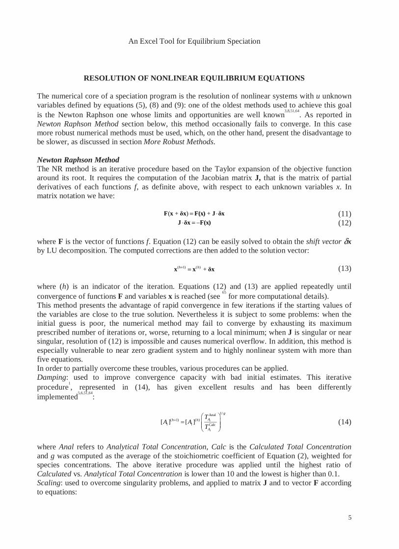
Newton Raphson Method section below, this method occasionally fails to converge. In this case more robust numerical methods must be used, which, on the other hand, present the disadvantage to be slower, as discussed in section More Robust Methods. Newton Raphson Method The NR method is an iterative procedure based on the Taylor expansion of the objective function around its root. It requires the computation of the Jacobian matrix J, that is the matrix of partial derivatives of each functions f, as definite above, with respect to each unknown variables x. In matrix notation we have: ( + ) + = ⋅F x δx F(x) J δx (11) ⋅ = −J δx F(x) (12) where F is the vector of functions f. Equation (12) can be easily solved to obtain the shift vector δx by LU decomposition. The computed corrections are then added to the solution vector: ( 1) ( ) + h h+ =x x δx (13) where (h) is an indicator of the iteration. Equations (12) and (13) are applied repeatedly until convergence of functions F and variables x is reached (see

65 for more computational details).

This method presents the advantage of rapid convergence in few iterations if the starting values of the variables are close to the true solution. Nevertheless it is subject to some problems: when the initial guess is poor, the numerical method may fail to converge by exhausting its maximum prescribed number of iterations or, worse, returning to a local minimum; when J is singular or near singular, resolution of (12) is impossible and causes numerical overflow. In addition, this method is especially vulnerable to near zero gradient system and to highly nonlinear system with more than five equations. In order to partially overcome these troubles, various procedures can be applied. Damping: used to improve convergence capacity with bad initial estimates. This iterative procedure

1, represented in (14), has given excellent results and has been differently

implemented5,6,51,64

:

1/Anal

( 1) ( )Calc

[ ] [ ] i

i

g

Ah hi i

A

TA A

T+

⎛ ⎞= ⎜ ⎟⎜ ⎟

⎝ ⎠

(14)

where Anal refers to Analytical Total Concentration, Calc is the Calculated Total Concentration and g was computed as the average of the stoichiometric coefficient of Equation (2), weighted for species concentrations. The above iterative procedure was applied until the highest ratio of Calculated vs. Analytical Total Concentration is lower than 10 and the lowest is higher than 0.1. Scaling: used to overcome singularity problems, and applied to matrix J and to vector F according to equations:


( ) 1/ 2*ab ab aa bbj j j j

−⋅ = ⋅ ⋅ (15) * * 1/ 2

a a aaf f j −= ⋅ (16) where *

abj and *af are the elements of the scaled matrix with dimensions u x u and vector

dimensions u, respectively3,51

. Convergence Forcer: another procedure used if initial estimates are not good. Divergence can be prevented viewing the process as a minimisation of the function g(x): 2

1

( ) (1/ 2) =(1/ 2) ( )u

ii

g x f x=

= ⋅ ∑TF F (17)

As the Newton step is in a descent direction for g(x), a good strategy is simply to find the value of a stepsize controller λ with a minimum located in the domain (0,1]. Equation (13) can be rewritten as: ( 1) ( ) + h h λ+ = ⋅x x δx (18) Although various approaches have been used to determine λ such as Hartley Method

3 and Cubic

Interpolation65, the following procedure is proposed in EST:

2

min

( , 0) ( , 1)

=

= -2 ( , 0)

- (2 )

g x g x

g x

κ λ λα κβ κ λλ β α

⎧ = = + =⎪⎪⎨

=⎪⎪ =⎩

(19)

which has been developed assuming a parabolic trend with a minimum of zero in the domain [0,1]. This formula presents the advantage that the evaluation of g(x) is needed only at the full NR step for λ=1. Step Limiter: as the NR procedure can determine negative concentrations (when δx < -x in (13)) it is necessary to restrict this step. This can be done using the approximation EXP(-ε) ~ (1 - ε), where ε is a small number. Equation (13) can be rewritten as suggested in

3:

( )( +1) ( )x x EXPh h xδ= ⋅ (20) This ensures that x

(h+1) ≥ 0.

Computation of Jacobian: the calculation of the Jacobian in EST has been implemented both algebraically and numerically by finite difference approximation. More Robust Methods Occasionally, despite the improvements described above, sometimes NR method fails, essentially becouse the initial estimates are too much different from the true values. For example, as far as a typical titration is concerned, this may occur at the start point, at the first addition, at an equivalence point, or when a phase appears or disappears. In these cases, a more robust approach to the resolution of equilibria equations is needed. Three common robust non-derivative methods have been here analysed: Simplex, Simulated Annealing and Genetic Algorithm. Our main aim was therefore to select a search method with good ability to escape from difficult local minima and zero-gradient region. In order to do that, Equation (17) has been therefore minimised.


7

Simplex Method The original Simplex Method was proposed by Spendley et al. in 1962

66 and enhanced in 1965 by

Nelder and Mead67 with a simple but powerful modification to the original method.

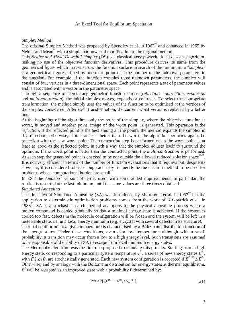
This Nelder and Mead Downhill Simplex (DS) is a classical very powerful local descent algorithm, making no use of the objective function derivatives. This procedure derives its name from the geometrical figure which moves across the function surface in search of the minimum: a “simplex” is a geometrical figure defined by one more point than the number of the unknown parameters in the function. For example, if the function contains three unknown parameters, the simplex will consist of four vertices in a three-dimensional space. Each point represents a set of parameter values and is associated with a vector in the parameter space. Through a sequence of elementary geometric transformations (reflection, contraction, expansion and multi-contraction), the initial simplex moves, expands or contracts. To select the appropriate transformation, the method simply uses the values of the function to be optimised at the vertices of the simplex considered. After each transformation, the current worst vertex is replaced by a better one. At the beginning of the algorithm, only the point of the simplex, where the objective function is worst, is moved and another point, image of the worst point, is generated. This operation is the reflection. If the reflected point is the best among all the points, the method expands the simplex in this direction, otherwise, if it is at least better than the worst, the algorithm performs again the reflection with the new worst point. The contraction step is performed when the worst point is at least as good as the reflected point, in such a way that the simplex adjusts itself to surround the optimum. If the worst point is better than the contracted point, the multi-contraction is performed. At each step the generated point is checked to be not outside the allowed reduced solution space

65,68.

It is not very efficient in terms of the number of function evaluations that it requires but, despite its slowness, it is considered robust enough and may frequently be the election method to be used for problems whose computational burden are small. In EST the Amoeba

65 version of DS is used, with some added improvements. In particular, the

routine is restarted at the last minimum, until the same values are three times obtained. Simulated Annealing The first idea of Simulated Annealing (SA) was introduced by Metropolis et al. in 1953

69 but the

application to deterministic optimisation problems comes from the work of Kirkpatrick et al. in 1983

70. SA is a stochastic search method analogous to the physical annealing process where a

molten compound is cooled gradually so that a minimal energy state is achieved. If the system is cooled too fast, defects in the molecule configuration will be frozen and the system will be left in a metastable state, i.e. in a local energy minimum (e.g. a crystal with several defects in its structure). Thermal equilibrium at a given temperature is characterised by a Boltzmann distribution function of the energy states. Under these conditions, even at a low temperature, although with a small probability, a transition may occur from a low to a high energy level. Such transitions are assumed to be responsible of the ability of SA to escape from local minimum energy states. The Metropolis algorithm was the first one proposed to simulate this process. Starting from a high energy state, corresponding to a particular system temperature T

(i), a series of new energy states E

(h),

with (h) ≥ (i), are stochastically generated. Each new system configuration is accepted if E(h+1)

≤ E(h)

. Otherwise, and by analogy with the Boltzmann distribution for energy states at thermal equilibrium, E

h will be accepted as an improved state with a probability P determined by:

( )( +1) ( ) ( )P=EXP -(E E ) / Th h i

BK− (21)


where T(i) is the current system temperature and K

B is Boltzmann's constant. At high temperatures

this probability is close to one, i.e. most energy transitions are permissible. As the system temperature decreases, the probability of accepting a higher energy state as being an improved energy state approaches zero, and it is assumed that thermal equilibrium is reached at each temperature. From an optimisation point of view, SA explores the key feature of the physical annealing process of generating transitions to higher energy states, applying to the new states an acceptance/rejection probability criterion which should naturally become more and more stringent with the progress of the procedure. For solving a particular problem with a SA algorithm, the following steps are thus necessary: (i) Definition of an objective function to be minimised. (ii) Adoption of an annealing cooling schedule, i.e. the initial temperature, the number of configurations generated at each temperature and a method to decrease the temperature itself must be specified. (iii) At each temperature in the cooling schedule, stochastic generation of the alternative combinations, centred on the currently accepted state must be made. (iv) Criteria for the acceptance or rejection of the alternative combinations, against the currently accepted state at that temperature, must be adopted. Three SA algorithms have been analysed with the proposal to select the best to be used in EST: SIMMAN

71, the hybrid SA-Simplex Amebsa

65 and a code developed in our laboratory (EST-SA).

The latter is based on Gaussian distribution with adaptive variance for the randomisation process and a variable length exponential cooling schedule

72,73. The variance for the randomisation process

and the exponential cooling schedule are driven by the rejection ratio with the Markov chain length set to four times the number of parameters

72.

Genetic Algorithms Genetic Algorithms (GA) are a group of mathematical techniques which were initially designed to simulate the behaviour of biologically based adaptive systems. Despite GA were not initially developed as an optimisation technique in itself, it can be modified to produce a powerful optimiser based on parallel search technique

74,75.

Introduced by Holland in 197576, it consists of an iterative procedure which mimics the evolutionary

process in nature. There are numerous variant of GA, but the classical architecture includes the three components Selection, Crossover and Mutation. It starts with a randomly selected population of potential solutions: each individual is characterised by a chromosome composed by genes in which the parameters are encoded. The initial population, by means of Genetic Operators, undergoes a simulated evolution, which copies the natural selective reproduction scheme, ‘survival of the fittest’. The Fitness of the individual is estimated by the objective function, which plays the role of an environment. This Fitness is then used to direct the application of the operations, which produces a new population (a New Generation). The new population is formed by selecting chromosomes with a probability relative to their Fitness (Selection). As this reproduction rule can lead to a decrease of chromosome diversity in the next few generations, the two genetic operators, Mutation and Crossover are introduced to counterbalance this phenomenon. Mutation works on the single genes level by changing at random single gene of individuals, with the probability of this event usually being very small. Crossover, the recombination operator of GA, is the main variation operator which hopefully recombines useful genes from different individuals. The Crossover Rate indicates the probability per individual to undergo recombination. Then with the two parent individuals, selected (at random) from the population, crossover forms two new offspring individuals. The new population of chromosomes is again individually evaluated and transformed into a subsequent generation. This process continues until convergence within a population is achieved.


9

EST-GA has been developed from the skeleton of Genetik77 of which the general scheme is hold

with a floating point representation. From this program, our GA maintains also the Elitist Strategy (the preservation of the best solution during the application of genetic operators), the Tournament Selection and the Whole Linear Crossover. The routine incorporates numerous suggestions from the works of Brunetti

78 and Nikitas

79,80.

EST-GA has been improved using a Gaussian distribution for the Generation of New Individuals; the standard deviation of the genes in the new individuals is controlled by hits in the last generation: if a success is gained in objective function reduction, the standard deviation is doubled, otherwise is halved. This enhances the capability of exploration and convergence. The Mutation Probability is controlled by the variance of population; this ensures an adequate element of random search while mutation becomes more productive and crossover less productive, as the population converges. Finally the whole population is replaced (with the exception of the best individual) if there is no improvement for a predetermined number of generations. The termination also occurs when there is no improvement after a fixed number of cycles. Main genetic parameters in EST-GA are Population of 50 individual, Crossover Probability of 0.85 and Mutation Probability of 0.01-0.1. To improve convergence capacity, all SA and the GA have been hybridised with Amoeba so the results of the former method give the seed of the latter one. In addition, for the sake of completeness, the relative performance of LM and NR methods heve been analysed by implementing the routines Mrqmin and Newt

65 as VBA code and by using a simplified version of

EST-NR algorithm. Finally, some other common used optimisation algorithms, such as the Powell’s Quadratically Convergent Direction Set Method in Multidimensions, the Conjugate Gradient Fletcher-Reeves-Polak-Ribiere Minimisation (FRPR), and the Broyden-Fletcher-Goldfarb-Shanno variant of the Quasi-Newton Davidon-Fletcher-Powell Minimisation (BFGS)

65, have been taken into account but,

as their performances were found to be not satisfactory, they were dropped out. Other algorithms, such as the MINPACK libraries or TENSOLVE

57 have been analysed, but not

considered suitable for EST application, as they are based on very complicated globalisation strategies

81: on the contrary, our target was the building of a very flexible tool without black boxes.

Results of Tests on Computational Methods Tests on the reliability of analysed methods have been run on a large number of minimisation problems: among them, we only remember those carried out on functions such as Rosenbrock

68, on

sets of data from the nonlinear regression of Statistical Reference Dataset s(http://www.nist.gov/itl/div898/strd) of National Institute of Standards and Technology (NIST), such as the MGH10, and on a typical equilibrium problem here reported as ML. In TABLE 1 we report the results of only the last two representative tests. MGH10 is a nonlinear regression with a high level of difficulty. ML is a simple example of formation of chemical complex 1:1 with log β

ML = 10, total component concentration of each

component 1 mol dm-3, starting values in interval 10

-10 - 1 mol dm

-3 with uniform random probability

in the logarithmic range. This simple example underlines the problem of good initial guesses. The table reports the relative execution time, the successful ratio (defined as the number of located on solution with relative error less of 1%), the average (avLRE) and the standard deviation (sdLRE) of Log Relative Error (LRE):

10

q-cLRE=-log

c

⎛ ⎞⎜ ⎟⎜ ⎟⎝ ⎠

(22)


where q is the estimated value and c the correct value82. The definition of successful rate used here

is not the classical one, but it is useful because our objective is to obtain a procedure that can be used as seed for the NR routine.

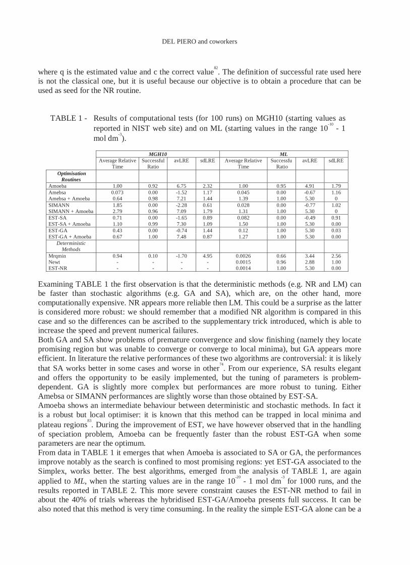
Examining TABLE 1 the first observation is that the deterministic methods (e.g. NR and LM) can be faster than stochastic algorithms (e.g. GA and SA), which are, on the other hand, more computationally expensive. NR appears more reliable then LM. This could be a surprise as the latter is considered more robust: we should remember that a modified NR algorithm is compared in this case and so the differences can be ascribed to the supplementary trick introduced, which is able to increase the speed and prevent numerical failures. Both GA and SA show problems of premature convergence and slow finishing (namely they locate promising region but was unable to converge or converge to local minima), but GA appears more efficient. In literature the relative performances of these two algorithms are controversial: it is likely that SA works better in some cases and worse in other

74. From our experience, SA results elegant

and offers the opportunity to be easily implemented, but the tuning of parameters is problem-dependent. GA is slightly more complex but performances are more robust to tuning. Either Amebsa or SIMANN performances are slightly worse than those obtained by EST-SA. Amoeba shows an intermediate behaviour between deterministic and stochastic methods. In fact it is a robust but local optimiser: it is known that this method can be trapped in local minima and plateau regions

83. During the improvement of EST, we have however observed that in the handling

of speciation problem, Amoeba can be frequently faster than the robust EST-GA when some parameters are near the optimum. From data in TABLE 1 it emerges that when Amoeba is associated to SA or GA, the performances improve notably as the search is confined to most promising regions: yet EST-GA associated to the Simplex, works better. The best algorithms, emerged from the analysis of TABLE 1, are again applied to ML, when the starting values are in the range 10

-20 - 1 mol dm

-3 for 1000 runs, and the

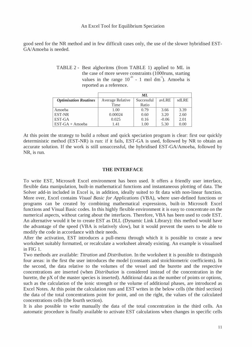
results reported in TABLE 2. This more severe constraint causes the EST-NR method to fail in about the 40% of trials whereas the hybridised EST-GA/Amoeba presents full success. It can be also noted that this method is very time consuming. In the reality the simple EST-GA alone can be a

TABLE 1 - Results of computational tests (for 100 runs) on MGH10 (starting values as reported in NIST web site) and on ML (starting values in the range 10

-10 - 1

mol dm-3).

MGH10 ML Average Relative

Time Successful

Ratio avLRE sdLRE Average Relative

Time Successfu

Ratio avLRE sdLRE

Optimisation Routines

Amoeba 1.00 0.92 6.75 2.32 1.00 0.95 4.91 1.79 Amebsa 0.073 0.00 -1.52 1.17 0.045 0.00 -0.67 1.16 Amebsa + Amoeba 0.64 0.98 7.21 1.44 1.39 1.00 5.30 0 SIMANN 1.85 0.00 -2.28 0.61 0.028 0.00 -0.77 1.02 SIMANN + Amoeba 2.79 0.96 7.09 1.79 1.31 1.00 5.30 0 EST-SA 0.71 0.00 -1.65 0.89 0.082 0.00 -0.49 0.91 EST-SA + Amoeba 1.10 0.99 7.30 1.09 1.50 1.00 5.30 0.00 EST-GA 0.43 0.00 -0.74 1.44 0.12 1.00 5.30 0.03 EST-GA + Amoeba 0.67 1.00 7.48 0.87 1.27 1.00 5.30 0.00

Deterministic Methods

Mrqmin 0.94 0.10 -1.70 4.95 0.0026 0.66 3.44 2.56 Newt - - - - 0.0015 0.96 2.88 1.00 EST-NR - - - - 0.0014 1.00 5.30 0.00


11

good seed for the NR method and in few difficult cases only, the use of the slower hybridised EST-GA/Amoeba is needed.

At this point the strategy to build a robust and quick speciation program is clear: first our quickly deterministic method (EST-NR) is run: if it fails, EST-GA is used, followed by NR to obtain an accurate solution. If the work is still unsuccessful, the hybridised EST-GA/Amoeba, followed by NR, is run.

THE INTERFACE

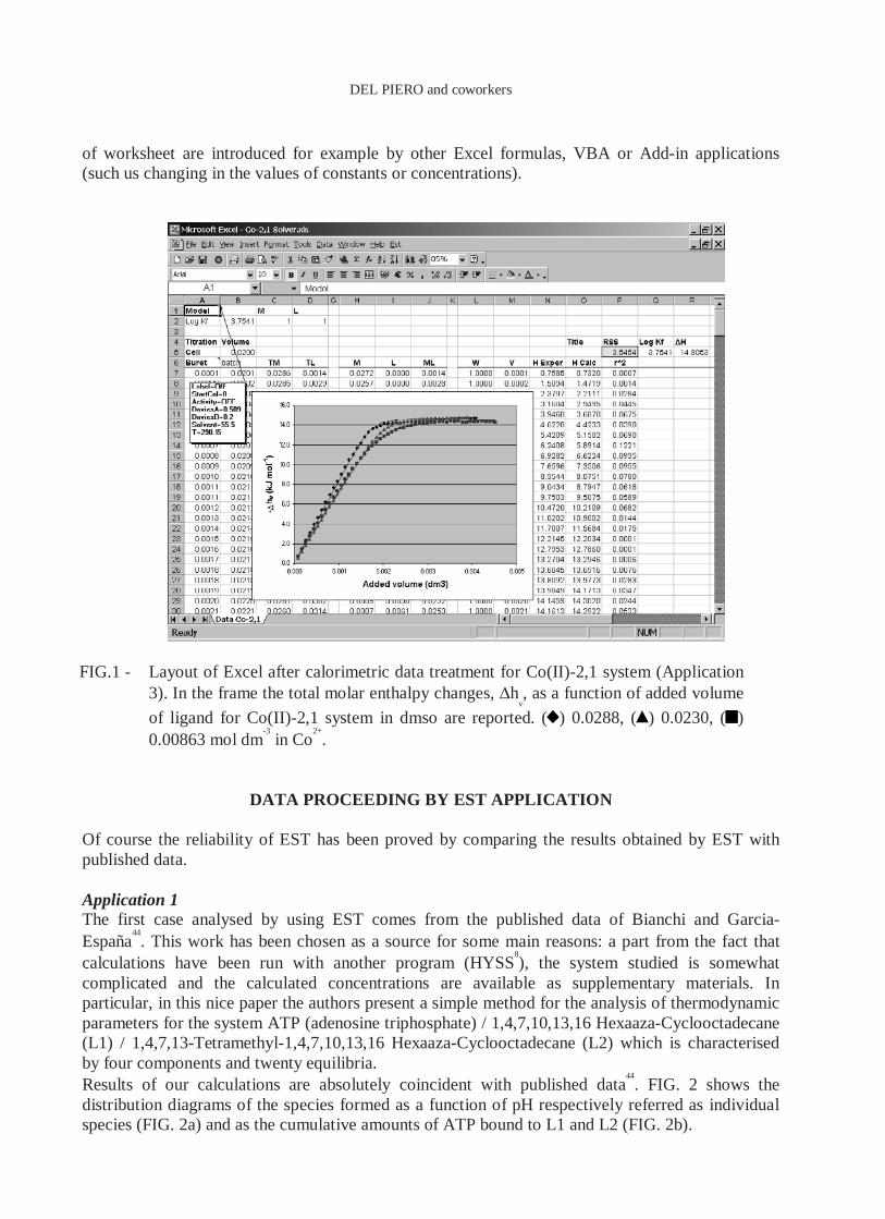
To write EST, Microsoft Excel environment has been used. It offers a friendly user interface, flexible data manipulation, built-in mathematical functions and instantaneous plotting of data. The Solver add-in included in Excel is, in addition, ideally suited to fit data with non-linear function. More over, Excel contains Visual Basic for Applications (VBA), where user-defined functions or programs can be created by combining mathematical expressions, built-in Microsoft Excel functions and Visual Basic codes. In this highly flexible environment it is easy to concentrate on the numerical aspects, without caring about the interfaces. Therefore, VBA has been used to code EST. An alternative would it be to create EST as DLL (Dynamic Link Library): this method would have the advantage of the speed (VBA is relatively slow), but it would prevent the users to be able to modify the code in accordance with their needs. After the activation, EST introduces a pull-menu through which it is possible to create a new worksheet suitably formatted, or recalculate a worksheet already existing. An example is visualised in FIG 1. Two methods are available: Titration and Distribution. In the worksheet it is possible to distinguish four areas: in the first the user introduces the model (constants and stoichiometric coefficients). In the second, the data relative to the volumes of the vessel and the burette and the respective concentrations are inserted (when Distribution is considered instead of the concentration in the burette, the pX of the master species is inserted). Additional data as the number of points or options, such as the calculation of the ionic strength or the volume of additional phases, are introduced as Excel Notes. At this point the calculation runs and EST writes in the below cells (the third section) the data of the total concentrations point for point, and on the right, the values of the calculated concentrations cells (the fourth section). It is also possible to write manually the data of the total concentration in the third cells. An automatic procedure is finally available to activate EST calculations when changes in specific cells

TABLE 2 - Best alghoritms (from TABLE 1) applied to ML in the case of more severe constraints (1000runs, starting values in the range 10

-20 - 1 mol dm

-3). Amoeba is

reported as a reference.

ML Optimisation Routines Average Relative

Time Successful

Ratio avLRE sdLRE

Amoeba 1.00 0.79 3.66 3.39 EST-NR 0.00024 0.60 3.20 2.60 EST-GA 0.025 0.16 -0.06 2.01 EST-GA + Amoeba 1.41 1.00 5.30 0.00


of worksheet are introduced for example by other Excel formulas, VBA or Add-in applications (such us changing in the values of constants or concentrations).

FIG.1 - Layout of Excel after calorimetric data treatment for Co(II)-2,1 system (Application 3). In the frame the total molar enthalpy changes, ∆h

v, as a function of added volume

of ligand for Co(II)-2,1 system in dmso are reported. ( ) 0.0288, ( ) 0.0230, ( ) 0.00863 mol dm

-3 in Co

2+.

DATA PROCEEDING BY EST APPLICATION

Of course the reliability of EST has been proved by comparing the results obtained by EST with published data. Application 1 The first case analysed by using EST comes from the published data of Bianchi and Garcia-España

44. This work has been chosen as a source for some main reasons: a part from the fact that

calculations have been run with another program (HYSS8), the system studied is somewhat

complicated and the calculated concentrations are available as supplementary materials. In particular, in this nice paper the authors present a simple method for the analysis of thermodynamic parameters for the system ATP (adenosine triphosphate) / 1,4,7,10,13,16 Hexaaza-Cyclooctadecane (L1) / 1,4,7,13-Tetramethyl-1,4,7,10,13,16 Hexaaza-Cyclooctadecane (L2) which is characterised by four components and twenty equilibria. Results of our calculations are absolutely coincident with published data

44. FIG. 2 shows the

distribution diagrams of the species formed as a function of pH respectively referred as individual species (FIG. 2a) and as the cumulative amounts of ATP bound to L1 and L2 (FIG. 2b).


13

4 6 8 10pH

0

0.0002

0.0004

0.0006

0.0008

0.001

Con

cent

ratio

n (m

ol d

m-3)

H3L13+

ATP4-

H3L23+

H5L1ATP+

H4ATPL1

H2L22+

L2

HL2+HL1+

H2L12+

H5ATPL2+

H4L14+H4ATPL23+

H3ATPL1-

H3ATPL2-

HATP3-

(a)

4 6 8 10

pH

0.0000

0.0002

0.0004

0.0006

0.0008

0.0010

(ATP)Tot

(L1ATP)Tot

(L2ATP)Tot

(b)

FIG.2 - Distribution of: (a) the individual species, (b) cumulative amounts of ATP bound to L1 and L2, for the system ATP/L1/L2 (Application 1).

The comparison with published data and figures proof the numerical reliability of EST referred to homogeneous chemical equilibria. Application 2 EST is here run on published data by Brown and Ebinger

45 where the authors examine four

precipitation problems which are solved to face the use of numerical equilibrium codes. This study emphasises concentrated solutions, assumes both ideal and non-ideal solutions, and employs different databases and different activity coefficient relationships. The study uses the EQ3/6 numerical speciation code

25. Results show satisfactory agreement between the solubility products

calculated from free-energy relationships and those calculated from concentrations and activity coefficients. The third precipitation problem analyzed in the paper

45 was solved with EST, that is the

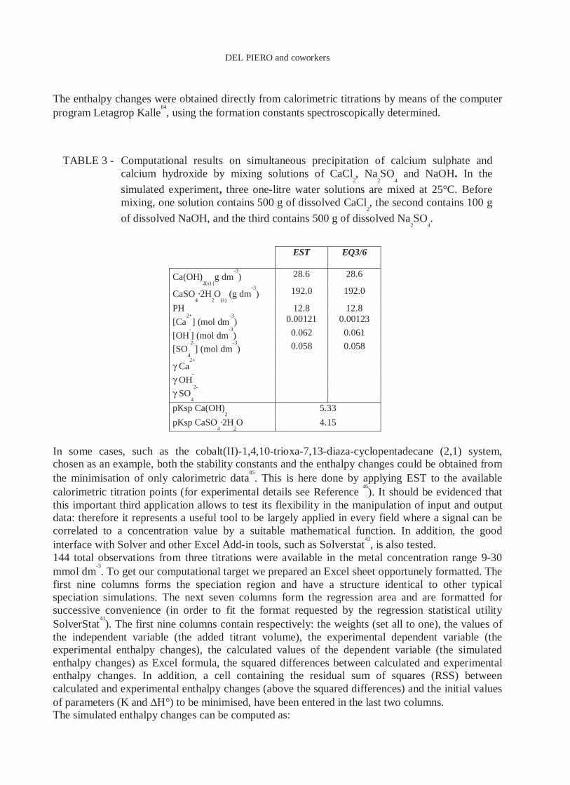
simultaneous precipitation of calcium sulphate and calcium hydroxide by mixing solutions of calcium chloride, sodium sulphate, and sodium hydroxide. This problem involves two precipitation equilibria and is therefore very suitable to test the relative computational algorithm for heterogeneous systems. The EST calculated concentrations of free and solid species are reported in TABLE 3 together with previous comparable data

45. The differences with published data are only

present in the last significative figure thus proving the reliability of EST also in the field of heterogeneous equilibria. For non-ideal solution the comparison was not significant as the concentrations considered by the authors were over the Davies equation range validity. Application 3 The third case studied by means of EST, takes advantage of same our data concerning the complex formation of Co(II) with mixed N/O ligands in dimethylsulfoxide (dmso)

46. In this previous work

the formation constants of CoLj complexes were obtained by means of UV-Vis spectrophotometric titrations, using Cd(II) as a competitive ion and analysing the data with the Hyperquad program

18.


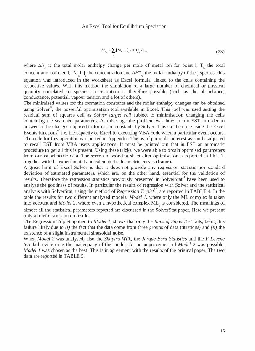
The enthalpy changes were obtained directly from calorimetric titrations by means of the computer program Letagrop Kalle

84, using the formation constants spectroscopically determined.

In some cases, such as the cobalt(II)-1,4,10-trioxa-7,13-diaza-cyclopentadecane (2,1) system, chosen as an example, both the stability constants and the enthalpy changes could be obtained from the minimisation of only calorimetric data

85. This is here done by applying EST to the available

calorimetric titration points (for experimental details see Reference 46). It should be evidenced that

this important third application allows to test its flexibility in the manipulation of input and output data: therefore it represents a useful tool to be largely applied in every field where a signal can be correlated to a concentration value by a suitable mathematical function. In addition, the good interface with Solver and other Excel Add-in tools, such as Solverstat

43, is also tested.

144 total observations from three titrations were available in the metal concentration range 9-30 mmol dm

-3. To get our computational target we prepared an Excel sheet opportunely formatted. The

first nine columns forms the speciation region and have a structure identical to other typical speciation simulations. The next seven columns form the regression area and are formatted for successive convenience (in order to fit the format requested by the regression statistical utility SolverStat

43). The first nine columns contain respectively: the weights (set all to one), the values of

the independent variable (the added titrant volume), the experimental dependent variable (the experimental enthalpy changes), the calculated values of the dependent variable (the simulated enthalpy changes) as Excel formula, the squared differences between calculated and experimental enthalpy changes. In addition, a cell containing the residual sum of squares (RSS) between calculated and experimental enthalpy changes (above the squared differences) and the initial values of parameters (K and ∆H°) to be minimised, have been entered in the last two columns. The simulated enthalpy changes can be computed as:

TABLE 3 - Computational results on simultaneous precipitation of calcium sulphate and calcium hydroxide by mixing solutions of CaCl

2, Na

2SO

4 and NaOH. In the

simulated experiment, three one-litre water solutions are mixed at 25°C. Before mixing, one solution contains 500 g of dissolved CaCl

2, the second contains 100 g

of dissolved NaOH, and the third contains 500 g of dissolved Na2SO

4.

EST EQ3/6

Ca(OH)2(s) (

g dm-3) 28.6 28.6

CaSO4·2H

2O

(s) (g dm

-3) 192.0 192.0

PH 12.8 12.8

[Ca2+

] (mol dm-3) 0.00121 0.00123

[OH-] (mol dm

-3) 0.062 0.061

[SO4

2-] (mol dm

-3) 0.058 0.058

γ Ca2+

γ OH-

γ SO4

2-

pKsp Ca(OH)2 5.33

pKsp CaSO4·2H

2O 4.15


15

0

m l M[M L ] Ti jv j

j

h Hβ∆ = ⋅ ∆∑ (23)

where ∆h

vi is the total molar enthalpy change per mole of metal ion for point i, T

M the total

concentration of metal, [MmL

l]

j the concentration and ∆H°

βj the molar enthalpy of the j species: this

equation was introduced in the worksheet as Excel formula, linked to the cells containing the respective values. With this method the simulation of a large number of chemical or physical quantity correlated to species concentration is therefore possible (such as the absorbance, conductance, potential, vapour tension and a lot of others). The minimised values for the formation constants and the molar enthalpy changes can be obtained using Solver

86, the powerful optimisation tool available in Excel. This tool was used setting the

residual sum of squares cell as Solver target cell subject to minimisation changing the cells containing the searched parameters. At this stage the problem was how to run EST in order to answer to the changes imposed to formation constants by Solver. This can be done using the Excel Events functions

42 i.e. the capacity of Excel to executing VBA code when a particular event occurs.

The code for this operation is reported in Appendix. This is of particular interest as can be adjusted to recall EST from VBA users applications. It must be pointed out that in EST an automatic procedure to get all this is present. Using these tricks, we were able to obtain optimised parameters from our calorimetric data. The screen of working sheet after optimisation is reported in FIG. 1. together with the experimental and calculated calorimetric curves (frame). A great limit of Excel Solver is that it does not provide any regression statistic nor standard deviation of estimated parameters, which are, on the other hand, essential for the validation of results. Therefore the regression statistics previously presented in SolverStat

43 have been used to

analyze the goodness of results. In particular the results of regression with Solver and the statistical analysis with SolverStat, using the method of Regression Triplet

87, are reported in TABLE 4. In the

table the results for two different analysed models, Model 1, where only the ML complex is taken into account and Model 2, where even a hypothetical complex ML

2 is considered. The meanings of

almost all the statistical parameters reported are discussed in the SolverStat paper. Here we present only a brief discussion on results. The Regression Triplet applied to Model 1, shows that only the Runs of Signs Test fails, being this failure likely due to (i) the fact that the data come from three groups of data (titrations) and (ii) the existence of a slight instrumental sinusoidal noise. When Model 2 was analysed, also the Shapiro-Wilk, the Jarque-Bera Statistics and the F Levene test fail, evidencing the inadequacy of the model. As no improvement of Model 2 was possible, Model 1 was chosen as the best. This is in agreement with the results of the original paper. The two data are reported in TABLE 5.


TABLE 4 - Regression analysis, parameter values and their errors as found by Excel Solver-

SolverStat for Model 1 and Model 2 in Application 3.

TABLE 5 - Thermodynamic parameters for Co(II)-2,1 system original and

calculated by applying EST (Application 3). The errors quoted correspond to three standard deviations

Statistical Parameters

Rejection

Valuesa

Model 1 Rejection

Valuesa

Model 2

Data Quality Passed Passed Model Quality ANOVA F value >3.91 8.37·10

5 >2.67 3.31·10

5

Runs-of-Signs Test <51 18 <59 10 Regression Method Quality

Shapiro Wilk Statistic >1.64 1.05 >1.64 3.35 Jarque-Bera Statistic >5.99 2.64 >5.99 7.39 F Value for Levene Test >3.91 1.09 >3.91 8.06 Model Selection RSS 3.54 2.95 R 0.999915 0.999929 95% CI for R 0.999882 - 0.999939 0.999901 - 0.999949

R2 0.999830 0.999859

R2

Adj 0.999829 0.999986

PRESS 3.62 3.11

R2

Prediction 0.999827 0.999851

AIC -3.68 -3.83

Calculated Model Parameters

tCritical

Value sb t

Calculated t

Critical Value s

b t

Calculated

Log KFML

>1.98 3.75 0.03 139.2 >1.98 3.63 0.03 110.0

∆H°ML

(kJ mol-1) >1.98 14.80 0.03 506.1 >1.98 15.16 0.08 199.3

Log KFML2

>1.98 >1.98 4.8 0.2 22.4

∆H°ML2

(kJ mol-1) >1.98 >1.98 13.1 0.6 23.1

a Critical Value selected for probability 5% and computed by SolverStat:

b Asymptotic

Standard Deviation for calculated parameters

Calculated Parameters

Original paper This work

Log KF

ML 3.7(0.2) 3.75(0.08)

-∆H°ML

(kJ mol-1) 14.8(0.2) 14.80(0.09)


17

CONCLUSIONS

The proposed powerful EST add-in, with the computational improvements here described, represents an innovative approach to the field of simulation of multicomponent/multiphase equilibria. It takes advantage of Microsoft Excel spreadsheet flexibility in order to obtain chemical-physical parameters both from simulated and experimental data, thus being of great help in the field of analytical chemistry. The great interest of EST lies also in its easiness and, particularly, in its ability to interact with other statistical, general purpose Excel tools, such as Solver and Solverstat, as clearly evidenced in this work: of course, only limited cases are analyzed here by using EST, being its range of application much wider than what can be proposed in a single paper. The computational methods developed in EST are shown to be very reliable also when applied to complicated homogeneous or heterogenous equilibrium systems. EST can be downloaded, free of charge, from the web site http://www.freewebs.com/solverstat/est/est.htm.

Received September 16th, 2005

Acknowledgements – This work has been supported by the Ministero dell'Istruzione, dell'Università e della Ricerca (MIUR, Rome) within the program COFIN 2002.

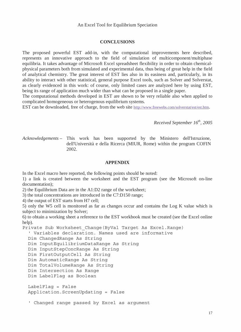
APPENDIX

In the Excel macro here reported, the following points should be noted: 1) a link is created between the worksheet and the EST program (see the Microsoft on-line documentation); 2) the Equilibrium Data are in the A1:D2 range of the worksheet; 3) the total concentrations are introduced in the C7:D150 range; 4) the output of EST starts from H7 cell; 5) only the W5 cell is monitored as far as changes occur and contains the Log K value which is subject to minimization by Solver; 6) to obtain a working sheet a reference to the EST workbook must be created (see the Excel online help). Private Sub Worksheet_Change(ByVal Target As Excel.Range) ' Variables declaration. Names used are informative Dim ChangedRange As String Dim InputEquilibriumDataRange As String Dim InputStepConcRange As String Dim FirstOutputCell As String Dim AutomaticRange As String Dim TotalVolumeRange As String Dim Intersection As Range Dim LabelFlag as Boolean LabelFlag = False Application.ScreenUpdating = False ' Changed range passed by Excel as argument


ChangedRange = Target.Address ' Set the EST working ranges AutomaticRange = "W5" InputEquilibriumDataRange = "A1:D2" InputStepConcRange = "C7:F150" FirstOutputCell = "H7" TotalVolumeRange = "" ' Test if the controlled range was changed Set Intersection = Application.Intersect(Range(AutomaticRange), _ Range(ChangedRange)) ' If the controlled range was unchanged then end the macro execution If Intersection Is Nothing Then Exit Sub End If Set Intersection = Nothing ' Prevents problem with calculation method of Excel If Application.Calculation <> xlCalculationAutomatic Then Application.Calculation = xlCalculationAutomatic End If ' This statement call the Speciation routine of EST workbook CallSpeciation InputEquilibriumDataRange, InputStepConcRange, _ FirstOutputCell, TotalVolumeRange, LabelFlag End Sub

REFERENCES

1) D.D. Perrin, I.G. Sayce, Talanta, 14, 833-842 (1967). 2) N. Ingri, W. Kakolowicz, L.G. Sillén, B. Warnqvist, Talanta, 14, 1261-1286 (1967). 3) I. Ting-Po, G.H. Nancollas, Anal. Chem., 44, 1940-1950 (1972). 4) G. Ginzburg, Talanta, 23, 149-152 (1976). 5) P.M. May, P.W. Linder, D.R. Williams, Dalton Trans., 588-595 (1977). 6) V.S. Tripathi, Talanta, 33, 1015-1020 (1986). 7) V.W.H. Leung, B.W. Darvell, A.P.C. Chan., Talanta, 35, 713-718 (1988). 8) L. Alderighi, P. Gans, A. Ienco, D. Peters, A. Sabatini, A. Vacca, Coord. Chem. Rev., 184, 311-

318 (1999). 9) K.J. Powell, L.D. Pettit, R.M. Town, K.I. Popov, University Chemistry Education, 4, 9-13

(2000), http://www.acadsoft.co.uk/soleq/soleq.htm. 10) N. Ingri, L.G. Sillén, Ark. Kemi, 23, 97 (1964). 11) R. Ekelund, L.G. Sillén, Wahlberg O., Acta Chem. Scand., 24, 3073 (1970).


19

12) R.J. Motekaitis, A.E. Martell, Can. J. Chem., 60, 168-173 (1982). 13) P. Gans, A. Sabatini, A. Vacca, Dalton Trans., 1195-1200 (1985). 14) J. Havel, M. Meloun, Talanta, 33, 525 (1986). 15) C. De Stefano, P. Mineo, C. Rigano, S. Sammartano, Ann. Chim. (Rome), 83, 243-277 (1993). 16) M. Kyvala, I. Lukes, Program for the Determination of Equilibrium Constants from

Potentiometric, Spectrophotometric, NMR, and Other Data, CHEMOMETRICS'95 - 4th International Chemometrics Conference of the Czech Chemical Society, Pardubice, Czech Republic (1995).

17) J. Barbosa, D. Barrón, J.L. Beltrán, V. Sanz-Nebot, Anal. Chim. Acta, 317, 75-81 (1995). 18) P. Gans, A. Sabatini, A. Vacca, Talanta, 43, 1739-1753 (1996),

http://www.hyperquad.co.uk/hq2000.htm. 19) N. Ingri, I. Andersson, L. Petterson, A. Yagasaki, L. Andersson, K. Holmström, Acta Chem.

Scand., 50, 717-734 (1996). 20) C.L. Araujo, A. Ibañez, G.N. Ledesma, G.M. Escandar, A.C. Olivieri, Comput. Chem., 22, 161-

168 (1998). 21) R. Cazallas, M.J. Citores, N. Etxebarria, L.A. Fernández, J.M. Madariaga, Talanta, 41, 1637-

1644 (1994). 22) J.C. Westall, J.L. Zachary, F.M.N. Morel, MINEQL: A Computer Program for the Calculation

of Chemical Equilibrium Composition of Aqueous Systems. Tech. Note no. 18. EPA Grant no. R-803738., Massachusetts Institute of Technology, Cambridge, MA, (1976).

23) J.W. Ball, D.K. Nordstrom, User's Manual for WATEQ4F, U.S.Geological Survey Report 91-183, (1991), http://wwwbrr.cr.usgs.gov/projects/GWC_chemtherm/software.htm.

24) J.D. Allison, D.S. Brown, K.J. Novo-Gradac, MINTEQA2/PRODEFA2, a Geochemical Assessment Model for Environmental Systems: Version 3.0 User's Manual., U.S.Environmental Protection Agency, Washington D.C., (1991), http://www.lwr.kth.se/English/OurSoftware/vminteq/index.htm.

25) T.J. Wolery, EQ3/6, A Software Package For Geochemical Modelling of Aqueous Systems: Package Overview and Installation Guide (Version 7.0), (1992).

26) D.L. Parkhurst, D.C. Thorstenson, L.N. Plummer, PHREEQE-a Computerized Program for Geochemical Calculations, U.S. Geological Survey, (1995).

27) D.L. Parkhurst, C.A.J. Appelo, User's guide to PHREEQC (Version 2) A computer program for speciation, batch-reaction, one-dimensional transport, and inverse geochemical calculations, U.S.Geological Survey Water-Resources Investigations Report 99-4259, (1999), http://wwwbrr.cr.usgs.gov/projects/GWC_coupled/phreeqc/index.html.

28) C.M. Bethke, Geochemical Reaction Modeling, Oxford University Press, New York, (1996), http://www.rockware.com/catalog/pages/gwb.html.

29) J. van der Lee, L. De Windt, CHESS Tutorial and Cookbook. User's Guide Nr. LHM/RD/99/05, CIG-École des Mines de Paris, Fontainebleau, France, (2000), http://chess.ensmp.fr.

30) D.A. Kulik, Am. J. Sci., 302, 227-279 (2002), http://les.web.psi.ch/Software/GEMS-PSI/. 31) R.P.T. Janssen, W. Verweij, Water Res., 37, 1320-1350 (2003). 32) G. Eriksson, Anal. Chim. Acta, 112, 375-383 (1979),

http://www.chem.umu.se/dep/inorgchem/samarbeta/WinSGW_eng.stm. 33) W.R. Smith, R.W. Missen, Chemical Reaction Equilibrium Analysis: Theory and Algorithms,

Krieger Publishing, Malabar, Florida, (1991), http://www.mathtrek.com/. 34) B. Müller, chemEQL, version 2.0. User's Guide to Application, Swiss Federal Institute of

Environmental Sciences and Technology (EAWAG), Dübendorf, Switzerland, (1996), http://www.eawag.ch/research/surf/forschung/chemeql.html.

35) P.M. May, Chem. Commun., 1265-1266 (2000). 36) D.N. Blauch, J. Chem. Inf. Comput. Sci., 42, 143-146 (2002).


37) L. Liwu, Java: Data Structures and Programming, Springer, New York, (1998). 38) E.J. Billo, Excel for Chemists, A Comprehensive Guide, Wiley-VCH, New York, (1997). 39) N. Maleki, B. Haghighi , A. Safavi, Microchem. J., 62, 229-236 (1999). 40) R. De Levie, Excel in Analytical Chemistry, University Press, Cambridge, (2001). 41) O. Raguin, A. Gruaz-Gruion, J. Barbet, Anal. Biochem., 310, 1-14 (2002). 42) J. Walkenbach, Excel 2003 Bible, Wiley Publishing, Indianapolis, (2003). 43) C. Comuzzi, P. Polese, A. Melchior, R. Portanova, M. Tolazzi, Talanta, 59, 67-80 (2003),

http://www.freewebs.com/solverstat/. 44) A. Bianchi, E. Garcia-España, J. Chem. Educ., 76, 1727-1732 (1999). 45) L.F. Brown, M.H. Ebinger, Comput. Chem., 22, 419-427 (1998). 46) S. Del Piero, A. Melchior, P. Polese, R. Portanova, M. Tolazzi, Dalton Trans., 1358-1365

(2004). 47) D.V. Nichita, S. Gomez, E. Luna, Comput. Chem. Eng., 26, 1703-1724 (2002). 48) P. Vonka, J. Leitner, Collect. Czech. Chem. Commun., 65, 1443-1454 (2000). 49) E.L. Cheluget, R.W. Missen, W.R. Smith, J. Phys. Chem., 91, 2428-2432 (1987). 50) D.J. Leggett, Talanta, 24, 535-542 (1977). 51) A. De Robertis, C. De Stefano, S. Sammartano, Anal. Chim. Acta, 191, 385-398 (1986). 52) R.N. Mioshi, C.L. do Lago, Anal. Chim. Acta, 334, 271-278 (1996). 53) P. Brassard, P. Bodurtha, Comput. Geosci., 26, 277-291 (2000). 54) G. Colonna, A. D'Angola, Comput. Phys. Commun., 163, 177-190 (2004). 55) E. Marengo, M.C. Gennaro, Analusis, 20, 345-350 (1992). 56) P.J. Vaughan, Soil Sci. Soc. Am. J., 66, 474-478 (2002). 57) A. Holstad, Comput. Geosci., 3, 229-257 (1999). 58) Y.K. Rao, Mar. Chem., 70, 61-78 (2000). 59) R. De Levie, J. Chem. Educ., 76, 987-991 (1999). 60) R. De Levie, J. Electroanal. Chem., 323, 347-355 (1992). 61) C.W. Davies, Ion Association, Butterworths, Washington, (1962). 62) J.M. Casas, F. Alvarez, L. Cifuentes, Chem. Eng. Sci., 55, 6223-6234 (2000). 63) D.W. King, J. Chem. Educ., 79, 1135-1140 (2002). 64) R. Tauler, E. Casassas, Anal. Chim. Acta, 206, 189-202 (1988). 65) W.H. Press, S.A. Teukolsky, W.T. Vetterling, B.P. Flannery, Numerical Recipes in C: The Art

of Scientific Computing, Cambridge University Press, Cambridge, (1992). 66) W.H. Spendley, G.R. Hext, F.R. Himsworth, Technometrics, 4, 441-461 (1962). 67) J.A. Nelder, R. Mead, Comput. J., 7, 308-315 (1965). 68) R. Chelouah, P. Siarry, Eur. J. Oper. Res., 148, 335-348 (2003). 69) N. Metropolis, M.N. Rosenbluth, A.W. Rosenbluth, A.H. Teller, E. Teller, J. Chem. Phys., 21,

1087-1092 (1953). 70) S. Kirkpatrick, C.D. Gellat Jr, M.P. Vecchi, Science, 220, 671-680 (1983). 71) W.L. Goffe, Studies in Nonlinear Dynamics and Econometrics, 1, 169-176 (1996). 72) V. Stark, Thesis: Implementation Of Simulated Annealing Optimization Method for APLAC

Circuit Simulator, Helsinki University of Technology, (1996). 73) M.F. Cardoso, R.L. Salcedo, S.F. Azevedo, Comput. Chem. Eng., 20, 1065-1080 (1996). 74) A.P. Alves da Silva, Learning Nonliner Models, 1, 45-60 (2002). 75) R.W. Wehrens, L.M.C. Buydens, Trac-Trends Anal. Chem., 17, 193-203 (1998). 76) J.H. Holland, Adaptation in Natural and Artificial Systems, University of Michigan Press, Ann

Arbor, (1975). 77) N. Turkkan, Discrete Optimization of Structures Using a Floating-Point Genetic Algorithm,

Annual Conference of the Canadian Society for Civil Engineering, Moncton, N.B., Canada, June 4-7 (2003), http://www.umoncton.ca/turk/logic.htm.


21

78) A. Brunetti, Comput. Phys. Commun., 124, 204-211 (2000). 79) P. Nikitas, A. Pappa-Louisi, A. Papageorgiou, A. Zitrou, J. Chromatogr. ,A, 942, 93-105

(2002). 80) P. Nikitas, A. Papageorgiou, Comput. Phys. Commun., 141, 225-229 (2001). 81) E. Bodon, L. Luksan, E. Spedicato, Numerical Performance of ABS Codes for Nonlinear Least

Squares, Tech. Rep. DMSIA 27/2001, Università degli Studi di Bergamo, Bergamo, (2001). 82) B.D. McCullough, Am. Stat., 52, 358-366 (1998). 83) M. Maeder, Y.M. Neuhold, G. Puxty, Chemometrics Intell. Lab. Syst., 70, 193-203 (2004). 84) R. Arnek, Ark. Kemi, 32, 81 (1970). 85) J.K. Grime, Analytical Solution Calorimetry, John Wiley & Sons, New York, (1985). 86) S. Wash, D. Diammond, Talanta, 42, 561-572 (1995). 87) M. Meloun, J. Militky, K. Kupka, R.G. Brereton, Talanta, 27, 721-740 (2002).

Documents

A NOVEL MULTIPURPOSE EXCEL TOOL FOR EQUILIBRIUM SPECIATION