A novel robust chance constrained possibilistic

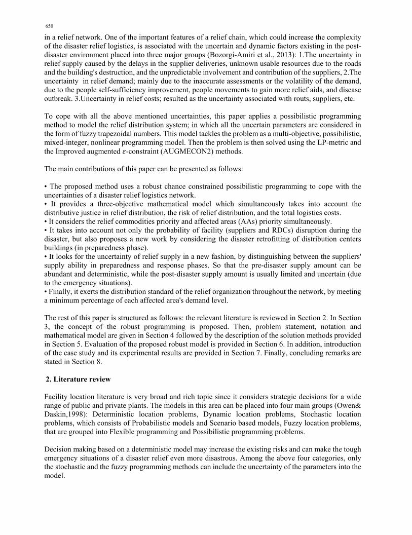
* Corresponding author. E-mail: [email protected] (M. Alinaghian) © 2016 Growing Science Ltd. All rights reserved. doi: 10.5267/j.ijiec.2016.3.001

International Journal of Industrial Engineering Computations 7 (2016) 649–670

Contents lists available at GrowingScience

International Journal of Industrial Engineering Computations

homepage: www.GrowingScience.com/ijiec

A novel robust chance constrained possibilistic programming model for disaster relief logistics under uncertainty

Maryam Rahafrooz and Mahdi Alinaghian*

Department of Industrial and Systems Engineering, Isfahan University of Technology, 84156-83111 Isfahan, Iran C H R O N I C L E A B S T R A C T

Article history: Received November 4 2015 Received in Revised Format December 21 2015 Accepted February 25 2016 Available online February 25 2016

In this paper, a novel multi-objective robust possibilistic programming model is proposed, which simultaneously considers maximizing the distributive justice in relief distribution, minimizing the risk of relief distribution, and minimizing the total logistics costs. To effectively cope with the uncertainties of the after-disaster environment, the uncertain parameters of the proposed model are considered in the form of fuzzy trapezoidal numbers. The proposed model not only considers relief commodities priority and demand points priority in relief distribution, but also considers the difference between the pre-disaster and post-disaster supply abilities of the suppliers. In order to solve the proposed model, the LP-metric and the improved augmented ε-constraint methods are used. Second, a set of test problems are designed to evaluate the effectiveness of the proposed robust model against its equivalent deterministic form, which reveales the capabilities of the robust model. Finally, to illustrate the performance of the proposed robust model, a seismic region of northwestern Iran (East Azerbaijan) is selected as a case study to model its relief logistics in the face of future earthquakes. This investigation indicates the usefulness of the proposed model in the field of crisis.

© 2016 Growing Science Ltd. All rights reserved

Keywords: Disaster relief Logistics Relief facility location Uncertainty Chance constrained possibilistic programming Robust optimization Multi-objective optimization

1. Introduction

A disaster is an unscheduled, overwhelming incident in association of people with their environment causing death, injury, and extensive casualties (Rubin et al., 1985). Disasters can be categorized as natural and man-made. Examples of the first one includes earthquake, flood, storm, drought, hurricanes and terrorist attacks, chemical leakages are some instances of man-made (Caunhye et al. 2012). From 2000 to 2007, the number of reported natural disasters around the world was approximately 460 disasters per year, which cost between 100 million and 400 million victims per year (Haghani & Afshar, 2009). Although natural disasters are unexpected, their damages can be minimized with proper preventive plans. Relief distribution center (RDC) location and relief distribution are among important strategies to improve the relief performance, since the numbers and the locations of RDCs, and the amount of supplies pre-positioned in them will directly affect the response time and the cost of logistics. So, this creates motivation to model the RDC location, and the inventory decisions associated with the relief distribution

650

in a relief network. One of the important features of a relief chain, which could increase the complexity of the disaster relief logistics, is associated with the uncertain and dynamic factors existing in the post-disaster environment placed into three major groups (Bozorgi-Amiri et al., 2013): 1.The uncertainty in relief supply caused by the delays in the supplier deliveries, unknown usable resources due to the roads and the building's destruction, and the unpredictable involvement and contribution of the suppliers, 2.The uncertainty in relief demand; mainly due to the inaccurate assessments or the volatility of the demand, due to the people self-sufficiency improvement, people movements to gain more relief aids, and disease outbreak. 3.Uncertainty in relief costs; resulted as the uncertainty associated with routs, suppliers, etc. To cope with all the above mentioned uncertainties, this paper applies a possibilistic programming method to model the relief distribution system; in which all the uncertain parameters are considered in the form of fuzzy trapezoidal numbers. This model tackles the problem as a multi-objective, possibilistic, mixed-integer, nonlinear programming model. Then the problem is then solved using the LP-metric and the Improved augmented -constraint (AUGMECON2) methods. The main contributions of this paper can be presented as follows: • The proposed method uses a robust chance constrained possibilistic programming to cope with the uncertainties of a disaster relief logistics network. • It provides a three-objective mathematical model which simultaneously takes into account the distributive justice in relief distribution, the risk of relief distribution, and the total logistics costs. • It considers the relief commodities priority and affected areas (AAs) priority simultaneously. • It takes into account not only the probability of facility (suppliers and RDCs) disruption during the disaster, but also proposes a new work by considering the disaster retrofitting of distribution centers buildings (in preparedness phase). • It looks for the uncertainty of relief supply in a new fashion, by distinguishing between the suppliers' supply ability in preparedness and response phases. So that the pre-disaster supply amount can be abundant and deterministic, while the post-disaster supply amount is usually limited and uncertain (due to the emergency situations). • Finally, it exerts the distribution standard of the relief organization throughout the network, by meeting a minimum percentage of each affected area's demand level. The rest of this paper is structured as follows: the relevant literature is reviewed in Section 2. In Section 3, the concept of the robust programming is proposed. Then, problem statement, notation and mathematical model are given in Section 4 followed by the description of the solution methods provided in Section 5. Evaluation of the proposed robust model is provided in Section 6. In addition, introduction of the case study and its experimental results are provided in Section 7. Finally, concluding remarks are stated in Section 8. 2. Literature review Facility location literature is very broad and rich topic since it considers strategic decisions for a wide range of public and private plants. The models in this area can be placed into four main groups (Owen& Daskin,1998): Deterministic location problems, Dynamic location problems, Stochastic location problems, which consists of Probabilistic models and Scenario based models, Fuzzy location problems, that are grouped into Flexible programming and Possibilistic programming problems. Decision making based on a deterministic model may increase the existing risks and can make the tough emergency situations of a disaster relief even more disastrous. Among the above four categories, only the stochastic and the fuzzy programming methods can include the uncertainty of the parameters into the model.

M. Rahafrooz and M. Alinaghian / International Journal of Industrial Engineering Computations 7 (2016)

651

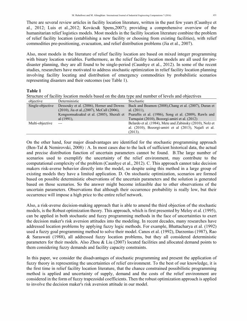
There are several review articles in facility location literature, written in the past few years (Caunhye et al., 2012; Luis et al.,2012; Kovács& Spens,2007); providing a comprehensive overview of the humanitarian relief logistics models. Most models in the facility location literature combine the problem of relief facility location (establishing a new facility or choosing from existing facilities), with relief commodities pre-positioning, evacuation, and relief distribution problems (Jia et al., 2007). Also, most models in the literature of relief facility location are based on mixed integer programming with binary location variables. Furthermore, as the relief facility location models are all used for pre-disaster planning, they are all found to be single-period (Caunhye et al., 2012). In some of the recent studies, researchers have motivated to address stochastic optimization in relief facility location planning involving facility locating and distribution of emergency commodities by probabilistic scenarios representing disasters and their outcomes (see Table 1). Table 1 Structure of facility location models based on the data type and number of levels and objectives

objective Deterministic Stochastic Single-objective Dessouky et al. (2006), Horner and Downs

(2010), Jia et al.,(2007), McCall (2006), Kongsomsaksakul et al. (2005), Sherali et al (1991),

Back and Beamon (2008),Chang et al. (2007), Duran et al. (2011), Psaraftis et al. (1986), Song et al. (2009), Rawls and Turnquist (2010), Bozorgi-amiri et al. (2012)

Multi-objective --- Belardo et al. (1984), Mete and Zabinsky (2010), Nolz et al. (2010), Bozorgi-amiri et al (2013), Najafi et al. (2013).

On the other hand, four major disadvantages are identified for the stochastic programming approach (Ben-Tal & Nemirovski, 2008) : A. In most cases due to the lack of sufficient historical data, the actual and precise distribution function of uncertain parameters cannot be found. B.The large number of scenarios used to exemplify the uncertainty of the relief environment, may contribute to the computational complexity of the problem (Caunhye et al., 2012). C. This approach cannot take decision makers risk-averse behavior directly into the model, so despite using this method in a large group of existing models they have a limited application. D. On stochastic optimization, scenarios are formed based on possible deterministic observations of the uncertain parameters and the solution is generated based on those scenarios. So the answer might become infeasible due to other observations of the uncertain parameters. Observations that although their occurrence probability is really low, but their occurrence will impose a high price to the entire relief network. Also, a risk-averse decision-making approach that is able to amend the third objection of the stochastic models, is the Robust optimization theory. This approach, which is first presented by Meloy et al. (1995), can be applied in both stochastic and fuzzy programming methods in the face of uncertainties to exert the decision maker's risk aversion attitudes into the modeling. In recent decades, many researches have addressed location problems by applying fuzzy logic methods. For example, Bhattacharya et al. (1992) used a fuzzy goal programming method to solve their model. Canos et al. (1992), Darzentas (1987), Rao & Saraswati (1988), all addressed fuzzy location problems, but they all considered deterministic parameters for their models. Also Zhou & Liu (2007) located facilities and allocated demand points to them considering fuzzy demands and facility capacity constraints. In this paper, we consider the disadvantages of stochastic programming and present the application of fuzzy theory in representing the uncertainties of relief environment. To the best of our knowledge, it is the first time in relief facility location literature, that the chance constrained possibilistic programming method is applied and uncertainty of supply, demand and the costs of the relief environment are considered in the form of fuzzy trapezoidal coefficients. Then the robust optimization approach is applied to involve the decision maker's risk aversion attitude in our model.

652

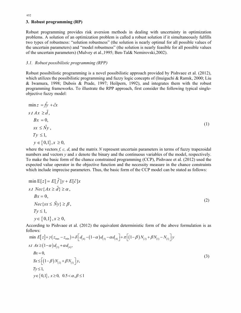
3. Robust programming (RP) Robust programming provides risk aversion methods in dealing with uncertainty in optimization problems. A solution of an optimization problem is called a robust solution if it simultaneously fulfills two types of robustness: “solution robustness” (the solution is nearly optimal for all possible values of the uncertain parameters) and “model robustness” (the solution is nearly feasible for all possible values of the uncertain parameters) (Mulvey et al.,1995; Ben-Tal& Nemirovski,2002). 3.1. Robust possibilistic programming (RPP) Robust possibilistic programming is a novel possibilistic approach provided by Pishvaee et al. (2012), which utilizes the possibilistic programming and fuzzy logic concepts of (Inuiguchi & Ramık, 2000; Liu & Iwamura, 1998; Dubois & Prade, 1997; Heilpern, 1992), and integrates them with the robust programming frameworks. To illustrate the RPP approach, first consider the following typical single-objective fuzzy model:

min

. ,

0,

,

1,

0,1 , 0,

z fy cx

s t Ax d

Bx

sx Ny

Ty

y x

(1)

where the vectors f, c, d, and the matrix N represent uncertain parameters in terms of fuzzy trapezoidal numbers and vectors y and x denote the binary and the continuous variables of the model, respectively. To make the basic form of the chance constrained programming (CCP), Pishvaee et al. (2012) used the expected value operator in the objective function and the necessity measure in the chance constraints which include imprecise parameters. Thus, the basic form of the CCP model can be stated as follows:

min E[ ] [ ] [ ]

. { } ,

0,

{ } ,

1,

0,1 , 0,

z E f y E c x

s t Nec Ax d

Bx

Nec sx Ny

Ty

y x

(2)

According to Pishvaee et al. (2012) the equivalent deterministic form of the above formulation is as follows:

max min 4 3 4 2 1 1

3 4

2 1

min 1 1

. 1 ,

0,

1 ,

1,

0,1 , 0, 0.5 , 1

E z z z d d d N N N y

s t Ax d d

Bx

Sx N N y

Ty

y x

(3)


653

where the first term in the objective function is the expected value of the objective function of model 1, which is the minimization of the expected total performance of the concerned system. The second term, i.e. , denotes the difference between the two extreme possible values of z. This term controls the solution robustness of the solution vector by minimizing the maximum deviation over and under the expected optimal value of z. In other words, is associated with the weight (importance) of this term against the two other terms of the objective function and and are defined as follows:

max 4 4z f y c x (4)

min 1 1z f y c x (5)

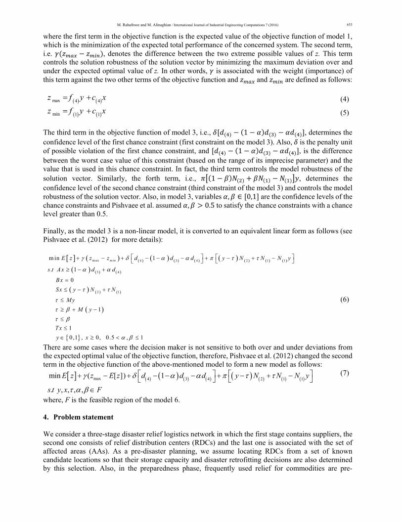
The third term in the objective function of model 3, i.e., 1 , determines the confidence level of the first chance constraint (first constraint on the model 3). Also, is the penalty unit of possible violation of the first chance constraint, and 1 , is the difference between the worst case value of this constraint (based on the range of its imprecise parameter) and the value that is used in this chance constraint. In fact, the third term controls the model robustness of the solution vector. Similarly, the forth term, i.e., 1 , determines the confidence level of the second chance constraint (third constraint of the model 3) and controls the model robustness of the solution vector. Also, in model 3, variables , ∈ 0,1 are the confidence levels of the chance constraints and Pishvaee et al. assumed , 0.5 to satisfy the chance constraints with a chance level greater than 0.5. Finally, as the model 3 is a non-linear model, it is converted to an equivalent linear form as follows (see Pishvaee et al. (2012) for more details):

m ax 4 3 4 2 1 1

3 4

2 1

m in 1

. 1

0

1

1

0,1 , 0, 0.5 , 1

m inE z z z d d d y N N N y

s t Ax d d

Bx

Sx y N N

M y

M y

Tx

y x

(6)

There are some cases where the decision maker is not sensitive to both over and under deviations from the expected optimal value of the objective function, therefore, Pishvaee et al. (2012) changed the second term in the objective function of the above-mentioned model to form a new model as follows:

max 4 3 4 2 1 1min ( 1

. ,

])

,

[

, ,

E z z d d d y N N NE y

s t x F

z

y

(7)

where, F is the feasible region of the model 6. 4. Problem statement We consider a three-stage disaster relief logistics network in which the first stage contains suppliers, the second one consists of relief distribution centers (RDCs) and the last one is associated with the set of affected areas (AAs). As a pre-disaster planning, we assume locating RDCs from a set of known candidate locations so that their storage capacity and disaster retrofitting decisions are also determined by this selection. Also, in the preparedness phase, frequently used relief for commodities are pre-

654

positioned in the selected RDCs to accelerate the after-disaster relief operations. In the response phase, we consider the commodity transportation from suppliers to RDCs, between RDCs (backup coverage) and from RDCs to the AAs. We make the following assumptions to model this problem: (1) The location of candidate RDC points and potential AA points are identified by the decision makers

before the planning time. (2) The capability of suppliers and RDCs might be partially disrupted by a disaster (3) The uncertainty of supply, demand and the costs of the relief environment are considered in terms

of trapezoidal fuzzy coefficients. (4) Three types of relief commodities (water/ food/ shelter) are supposed to be delivered so that each

type has its own volume and cost of procurement, storage, and transportation. (5) An RDC can be opened with only one of the three possible storage capacities, small, medium, large,

and seismic retrofitting levels (not retrofitted, partly retrofitted, totally retrofitted); subject to the associated setup cost.

(6) To ease the relief coordinations, each AA only serves with one RDC. (7) In the response phase, not only the commodity shortages in AAs, but also the excess inventory stored

in RDCs, are penalized. 4.1.Mathematical model

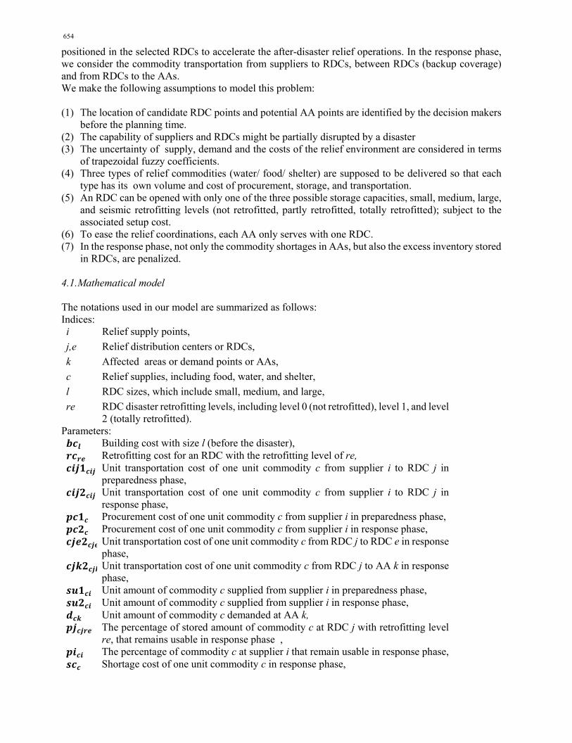
The notations used in our model are summarized as follows: Indices:

Relief supply points, i

Relief distribution centers or RDCs, j,e

Affected areas or demand points or AAs, k

Relief supplies, including food, water, and shelter, c

RDC sizes, which include small, medium, and large, l RDC disaster retrofitting levels, including level 0 (not retrofitted), level 1, and level 2 (totally retrofitted).

re

Parameters: Building cost with size l (before the disaster), Retrofitting cost for an RDC with the retrofitting level of re, Unit transportation cost of one unit commodity c from supplier i to RDC j in preparedness phase,

Unit transportation cost of one unit commodity c from supplier i to RDC j in response phase,

Procurement cost of one unit commodity c from supplier i in preparedness phase, Procurement cost of one unit commodity c from supplier i in response phase, Unit transportation cost of one unit commodity c from RDC j to RDC e in response phase, Unit transportation cost of one unit commodity c from RDC j to AA k in response phase, Unit amount of commodity c supplied from supplier i in preparedness phase, Unit amount of commodity c supplied from supplier i in response phase, Unit amount of commodity c demanded at AA k, The percentage of stored amount of commodity c at RDC j with retrofitting level re, that remains usable in response phase ,

The percentage of commodity c at supplier i that remain usable in response phase, Shortage cost of one unit commodity c in response phase,


655

Holding cost of one unit commodity c in RDCs, Required unit space for each unit of commodity c, The capacity of an opened RDC with size l (in cubic meters), Disaster risk index of RDC j based on its proximity to the center of the disaster, Importance factor of AA k based on its proximity to the center of the disaster, Importance factor of commodity c in the disaster, Distance between RDC j and AA k, An arc index for the path between RDC j and AA k, Big number in mathematical modeling, Integer numbers chosen by the decision maker , , Minimum percent of the demand of each AA that should be responded.

Variables: Amount of commodity c transferred from supplier i to RDC j in response phase, Amount of commodity c transferred from supplier i and pre-positioned at RDC j

in preparedness phase, Amount of c transferred from RDC j to AA k in response phase, Shortage amount of commodity c in AA k in response phase, Inventory amount of commodity c holding at RDC j in response phase, Amount of commodity c transferred from RDC j to RDC e, as a backup coverage,

in response phase 1 if an RDC with size l and retrofitting level re is located at candidate point RDC

j, 0 otherwise, 1 if RDC j sent commodity to AA k, 0 otherwise.

According to the robust chance constrained approach described in the previous section, the proposed model has the following form: First objective:

1min .maxck cjkj

c kk

c ck

d yz ifc ifk

d

(8)

The first objective function is associated with increasing the distributive justice in relief distribution. In this case, it minimizes the summation of weighted maximum relative lack of any kind of relief commodities in AAs, by considering the priority of each commodity type and the priority of each AA in relief distribution. It is the first time in disaster relief logistics, that the distributive justice in relief distribution is considered along with commodities’ priority and AA's priority in getting relief services. The linear form of this objective function in the form of chance constrained programming is as follows:

1 1maxmin .c cc

z ifc z

(9)

, ,

2max

1 3 1 4

.,

1C K C K

cjk kj

k c

ck ck

y ifkifk z c k

d d

(10)

As the Eq. (10) is a chance constraint, to provide model robustness of the solution vector, will be added to the final robust objective function:

, ,

1, 41 3 1 4

.1 1

( . ) ,1

).(C K C K

cjk kjc k ckck ck

CLCC y ifk c kdd d

(11)

Second objective is also as follows,

656

2 jk,

m in m axj k

z u

(12)

So that:

jk { ( }. . . . )jk jk k cjk c

c

u fjk djk ifk y ifc

(13)

The second objective minimizes the risk of relief distribution and implicitly increasing the relief distribution speed from RDCs to AAs. The linear form of this objective function is reported as the form of Eq. (14) to Eq. (18):

2 2 m axmin z z (14)2 max2 ,. .jk k jkdjk ifk g z j k (15)

(16)

12 ,.jk jkg M f jk j k (17)

1.2 ( ) 1 ,jk cjk c jk

c

g y ifc M fjk j k (18)

Third objective:

3 3 3minbefore after

z z z (19)

The third objective of the problem minimizes before and after disaster logistics costs. Eq. (20) consists of construction and retrofitting costs of the RDCs, procurement costs of the relief commodities and transportation cost of pre-positioning the relief commodities in RDCs in preparedness phase:

3, , , ,

( ) 1 1before l re ljre c cij cij cij

j l re c i j

z bc rc z pc q cij q (20)

3, , , , ,, ,

( 2 2 ) 2 2af ter c cij cij cij cje cje cjk cjk c cj

j e c j k c j cc i j

z pc x cij x cje v cjk y hc ih (21)

Also, Eq. (21) encompasses after disaster costs, such as procurement and transportation costs of the relief commodities throughout the network in response phase. According to the adopted robust chance constrained approach, the deterministic form of the third objective function is as follows:

3 3 3] [ ]min [before after

E z z E z (22)

In which we have:

, , , , ,3

, ,

[ (E[ 2 [ 2 )] ] ] [ 2 ] ][ 2after c ccij cij cij cje cje cjk cjk cj

j e c j k c j cc i j

E pc x E cij x E cje v E cjk y hc ihz

(23)Aaccording to Pishvaee et al. (2012), we can calculate the expected value of the fuzzy numbers of the above equation. In addition, constraints of the model are as follows, Constraint 1:

. ,cij cjre cij cej cje cjk cji ki e e

x pj q v v y ih c j (24)

This constraint controls the commodity balance of each RDC. In this constraint, the term cjrepjis obtained

from the following equation:

1 2

, 0 , 1 , 2

. . .1 1 1 ,cjre lre j lre j lre jl re level l re level l re level

pj z ri z ri z ri c j

. (25)

In order to linearize the Eq. (25), we define variables 1 2 3, ,cj cj cjw w w as follows:

1 0, 0

1cj ljlevel j cijl re level i

w z ri q

(26)

2 ( ) ,.jk cjk c

c

g y ifc j k


657

12 1

, 1


w z ri q

(27)

23 2

, 2


w z ri q

(28)

So that we have:

1 2 3.cjre cij cj cj cj

i

pj q w w w (29)

Accordingly the linear form of the first constraint is equivalent to Eqs. (30-41):

1 2 3 ,cij cj cj cj cej cje cjk cji e ke

x w w w v v y ih c j (30)

,

1ljrel re

z j (31)

1 2, 0

,cj ljrel re level

w M z c j

(32)

1 1 ,cj j cij

i

w ri q c j (33)

1 2, 0

1 1 ,cj j cij ljrei l re level

w ri q M z c j

(34)

2 2, 1

,cj ljrel re level

w M z c j

(35)

12 1 ,cj j cij

i

w ri q c j (36)

12 2

, 1

1 1 ,cj j cij ljrel re leveli

w ri q M z c j

(37)

3 2, 2

,cj ljrel re level

w M z c j

(38)

23 1 ,cj j cij

i

w ri q c j (39)

23 2

, 2

1 1 ,cj j cij ljrei l re level

w ri q M z c j

(40)

1 2 3, , 0 ,cj cj cjw w w c j (41)

Also, Eq. (31) ensures that at most one RDC can be constructed at each RDC candidate point. Constraint 2:

. ,cjk ckj

y d c k (42)

This constraint shows the relief organization standard in responding to the affected areas of demands and Eq. (43) shows its deterministic form:

(43)

Afterwards, 2CLCC will be added to the final robust objective function to fulfill model robustness of the

solution vector:

, ,2 4 2 3 2 4,

1c k c kck ck ck

c k

CLCC d d d (44)

Constraints 3-7:

, ,2 3 2 41 ,

c k c k

cjkjck ck

yd d c k

658

3,

,cje ljree j l re

v M z c j

(45)

3,

,cej ljree j l re

v M z c j

(46)

0 ,cje

e j

v c j

(47)

4,

,cij ljrei l re

x M z c j

(48)

5

,

,cjk ljre

k l re

y M z c j

(49)

Eq. (45) to Eq. (47) ensure having backup coverage between only any two established RDCs. Also, Eq. (48) prevents suppliers from transferring commodities to a not opened RDC and Eq. (49) guarantees sending commodities to AAs only from an opened RDC. Constraints 8-9:

, ,

.c cij l ljrec i l re

vo q cap z j (50)

,

.c cj l ljrec l re

vo ih cap z j (51)

These two constraints ensure that commodity pre-positioning and storing additional commodities in RDCs must be based on their storing capacities. Constraint 10:

1 ,cij cij

q su c i (52)

According to this constraint, in preparedness phase, the amount of commodity c procured from supplier i, cannot exceed the supplier's capacity. Constraint 11:

. 2 ,cij ci cij

x pi su c i (53)

This constraint ensures that, in response phase, the dispatched commodity from each supplier is limited by its usable inventory amount. Also, the deterministic form of this constraint, in chance constrained programming, is as follows:

, ,3 2 3 11 2 2 ,

c i c i

cijjck ck

ci

xsu su c i

pi

(54)

Moreover, in order to fulfill the model robustness of the solution vector, the term 3CLCC should be added

to the final robust objective function:

, ,3 3 2 3 1 1,

1 2 2 2c i c ick ck ck

c i

CLCC su su su

(55)

The commodity inventory of the suppliers in preparedness phase is supposed to be a deterministic parameter, Since before disaster they have enough time to procure and supply an abundant amount of commodities. While in response phase, as suppliers must emergently supply relief commodities, their commodity inventory is supposed to be a non-deterministic parameter. So suppliers' capabilities in procuring commodities are different in preparedness and response phases, while to the best of our knowledge, this note is ignored in all the previous studies in the disaster relief logistics literature. So that, in all the relief logistics models considering the uncertainty of the relief supply, the relief supply in preparedness phase and response phase are both supposed to be an uncertain parameters. Constraints 12-14:

(56)6 . ,cjk jk

c

y M fjk j k


659

(57)

(58)

According to the above three constraints, each AA allocates to exactly one RDC and receives reliefs only from its dedicated RDC. This allocation can also ease the relief coordinations while having backup coverage between the RDCs of the relief network. 5. Solution methods First, Lp-metric method is utilized, under which the proposed model becomes a single-objective problem and it enables us to evaluate the proposed robust model against its equivalent deterministic form.Then, in the next step, to provide a comprehensive sight of our three-objective problem, augmented -constraint method (AUGMECON2) is presented and this method is used to solve the case study. 5.1. LP-metric In this method, first, the optimal value of each objective function is calculated by solving the relevant one-objective problems. Then, a single objective function is employed to minimize the summation of normalized differences between each objective function and its optimal value, on the solution space of the multi-objective function (Soltani et al.,2015). We used this method by minimizing the following objective function on the solution space of our model:

* max max ** *3 3 3 3 3 31 1 2 2

1 2 3* * * max *1 2 3 3 3

41 , 3 1 , 4 4 3 , 3 3 ,

1 2

fina

,

3 4 4

l

,

[ ] ( [ ]) ( [ ]). . . [ ]

( [

0.

])

1 1

1 1

1 1

5 ( )

ckc k ck c k ck ck c k ck c k c

c k c k

ck ck ck

E z z z E z z E zz z z zz w w w

z z z z E z

dd d d d d

d d d

4

4 3 4

4 , 2 4 , 1 1

3, 2 1

0.5 ( )

0.

1 2 2 2

2 2 25 ( )

k

ck ck ck

c k ck c k ck ck

c i ck ck ck

d d d

su su su

su su su

)59(So that:

3 3

1 1

1i ii i

w

(60)

5.2. Improved augmented -constraint method (AUGMECON2) The -constraint method solves a multi-objective problem by optimizing one of the objective functions while using the other objective functions as constraints, incorporating them in the constraint part of the model. In order to apply this method, it is necessary to have the range of the objective functions used as constraints. Payoff table is a common approach to calculate these ranges. This table is made with the result of individual optimization of the objective functions while the nadir value is usually approximated with the minimum of the corresponding column (Steuer, 1986; Miettinen, 2012). For the implementation of the ordinary -constraint method two points must be considered: first, the range of the objective functions over the efficient set, mainly the calculation of nadir values. Second, the

,jk cjkc

fjk y c i 1jk

j

fjk k

660

guarantee of efficiency of the obtained solution (Mavrotas, 2009). To overcome these ambiguities, augmented -constraint method (AUGMECON) is proposed (Mavrotas, 2013). In AUGMECON method, lexicographic optimization is used to construct the payoff table with only Pareto-optimal solutions. There is a trade off between the density of the produced efficient set and the computation time, so we can control the density of the efficient set. In this method, in order to guarantee the efficiency of the obtained solution, the objective-function constraints are transformed to equalities by incorporating the appropriate slack or surplus variables. These slack or surplus variables are used as the second term, with lower priority in a lexicographic manner, in the objective function, forcing the program to produce only efficient solutions (Mavrotas, 2013). According to (Mavrotas, 2009), in the AUGMECON method the model is as follow,:

321

2 3

2 2 2 3 3 3

sssmax{ (

s s , s s

... )}

, ..., , ,

p

p

pp p i

f x

subject to f x e

r r r

x Sf x e f x Re

(61)

where is the RHS of the constrained objective functions, δ is a small number (usually ∈10 , 10 ). Also, in order to avoid any scaling problems, it is recommended to replace the (the

surplus variable of the i-th objective function) in the second term of the objective function, by / , where is the range of the i-th objective function (as calculated from the payoff table). In AUGMECON2, the improved version of AUGMECON, the objective function is slightly modified as follows (Mavrotas, 2013):

1 (21

2

2 2 2 3 3

2)3

3

3

(10 ..sss

max{ [ )

s s , s s

. (10 ) ]}

, ..., , ,

p

p

p

ip

p

p

f x

su

r r r

x Sbject to f Rx e f x e f x e

(62)

This modification is performed in order to perform a kind of lexicographic optimization on the rest of the objective functions, if there is any alternative optima. For example, with this formulation the solver will find the optimal for and then it will try to optimize , then , and so on. With the previous formulation the sequence of optimizations of was indifferent, while now we force the sequential optimization of the constrained objective functions (in case of alternative optima). In AUGMECON 2 like AUGMECON, for each objective function i=2…p the objective function range is calculated, then the range of the i-th objective function is divided into equal intervals, thus there would be total 1 grid points, that are used to vary parametrically the RHS of the i-th objective function. So the discretization step for this objective function is given as:

ii

i

rstep

q (63)

The RHS of the corresponding constraint in the k-th iteration in the specific objective function will be as Eq. (64), where is the minimum obtained from the payoff table and k is the counter for the specific objective function:

min ( ) 0,..., ik

i i istepe k kf q (64)

But in AUGMECON2, in each iteration, surplus variable that corresponds to the innermost objective function is checked. In this case it is the objective function with p=2. Then the bypass coefficient is calculated as:

2

2

int ( )s

bstep

(65)


661

where int() is the function that returns the integer part of a real number. When the surplus variable is larger than the , it is implied that in the next iteration the same solution will be obtained and the only difference is the surplus variable which will have the value . This makes the iteration redundant and therefore it can be bypassed as no new Pareto optimal solution is generated. The bypass coefficient b actually indicate how many consecutive iterations can be bypassed. Thus, in this way, especially when we have many grid points, AUGMECON2 method can significantly improve the Solution time (Mavrotas, 2013). Accordingly, our proposed model in AUGMECON2, forms as follows:

max23 3 3 1 1 2 2 3 3

2

1 1 1 2

1 ( 2)3

3

22

sssmax{ [ ] [ ) [ ]

s s

(10 ... (1

s

0 ) ] }

, , ,

p

p

i

pE z z E z CLCC CLCC CLCC

subject to f x e f x e

r r r

x S R

(66)where S is the feasible region of our proposed model. Also, the third objective function of our proposed model ( , is selected as the main objective function, and our first and the second objective functions are incorporated in its constraint part. Since our third objective function has fuzzy parameters, the expected value of it is used in the model Eq. (66). Other terms in the objective function of the above model, as described before, are related to solution robustness and model robustness of our proposed model. 6. Evaluation of the proposed robust model First, we assume a natural disaster such as an earthquake happens in the center of three concentric circles, consisting of an inner, middle, and outer circles. Second, the AA nodes are randomly placed in the inner circle, as the RDC nodes, and the supplier nodes are randomly generated in the middle and outer circles, respectively. Test problems are generated by randomly changing the values of some critical parameters such as the number of suppliers, the number of relief distribution centers, and the number of potentially affected areas. In addition we assume: Test problems are generated by randomly changing the number of suppliers, the number of RDCs and the number of potentially AAs. The number of suppliers is from 1 to 10, the number of RDCs is from 3 to 20, and the number of AAs is from 4 to 25. After locating the network nodes, parameters such as , , are estimated according to the Euclidean distance between these nodes and the earthquake epicenter, the disaster type, the disaster intensity, and urban fabrics. To generate the demand amounts, first the population of each AA is randomly generated. Then, water and food demands at each AA are estimated on the basis of the population, multiplied by the vulnerability probability ( ) of the AA. As the considered shelter has a capacity for accommodating three people, the estimated shelter demand at each AA is set to the number of affected people divided by three. Then, by the estimated demand amounts, we can generate the fuzzy trapezoidal demand numbers, as follows:

1 2 3 4 k, , , deman , ,d 0.7 0.9 1.1 , 1.3 .ck ck ck ck ckd d d dd (67)

Since there is usually sufficient time before disaster to supply an abundant amount of relief commodities, we estimate the pre-disaster total supply of each commodity to be about three times of its total estimated demand. The post-disaster supply amount is usually limited and uncertain, and we estimate it as follows:

4 3 )(

2supply numbe s

4r

ck ckk

ci

d d

S i

(68)

662

The above formula is used for generating the water and food amounts and one third of this amount is used as the shelter amount. Then, by the estimated post-disaster supply amounts, we can generate the fuzzy trapezoidal post-disaster supply numbers, as follows:

1 2 3 42 , 2 , 22 , , 1., 2 2 0.8 0.95 , .05 1.2ci ci ci ci ci cisu su su suu Ss (69)

To estimate the relief pre-disaster transportation costs, we multiply the inter-node Euclidean distances of our relief network to the unit transportation cost of each commodity. The post-disaster unit transportation costs are considered 1.2 times that of the pre-disaster. The fuzzy trapezoidal post-disaster transportation costs are defined as:

1 2 3 42 , 2 , 2 , 2 2 0.8 , 0.9 , 12 .1, 1.2 ,cij cij cij cij cij cijcij cij cij cij cici jj (70)

1 2 3 42 2 , 2 , 2 , 2 2 0.8 , 0.9 , 1.1, 1.2 ,cjk cjk cjk cjk cjk cjkcjk cjk cjk cjk cjk cjk (71)

1 2 3 42 2 , 2 , 2 , 2 2 0.8 , 0.9 , 1.1, 1.2 .cje cje cje cje cje cjecje cje cje cje cje cje (72)

As proposed by Bozorgi-Amiri et al. (2013), holding cost of a unit commodity in response phase can be estimated according to its procurement cost, and the post-disaster procurement cost of each commodity can be considered nearly equal to that of pre-disaster. So the fuzzy trapezoidal post-disaster procurement costs are estimated as follows:

1 2 3 42 2 , 2 , 2 , 2 1 0 .9 , 1 , 1 .1 , 1 .2c c c c c cp c p c p c p c p c p c (73) Accordingly, to evaluate the effectiveness of the proposed robust model against its equivalent deterministic form, the following steps are performed: 1. Five different test problems are randomly generated (as described before). 2. The problems are modeled based on both the robust and the deterministic forms. 3. Models are solved by LP-metric solution method, using GAMS 23.9 running on a PC Pentium IV-

5GHz with 4GB of RAM (DDR 3) under the Windows 7 environment. Moreover, for each problem, pre- disaster Strategic and tactical decisions, such as the location, size and retrofitting level of the RDCs, and the pre-positioned amount of commodities, are determined under both of its robust and deterministic models.

4. Ten different random scenarios are generated for each problem. A scenario is a specific realization of the uncertain parameters of a problem. So, each problem will be modeled in a deterministic form under each of its related scenarios.

5. Two surveys are conducted under each of the ten scenarios of a problem so that, each time, the pre disaster decisions adopted by solving one of the two models in step 3, are inserted as input parameters in the deterministic model made in step 4.

6. Deterministic models of step 4 are solved using LP-metric solution method and their result are used to evaluate the effectiveness of the robust approach.

Furthermore, it is assumed that the importance of the first and the second objectives are respectively four and three times the importance of the third objective. Also, it is assumed that the relief organization is planed to meet at least 90% of AA's demand.

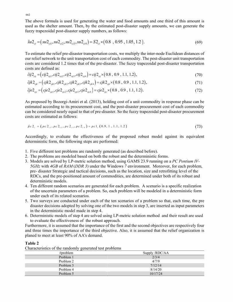
Table 2 Characteristics of the randomly generated test problems

#problem Supply /RDC/AA Problem 1 2/3/4 Problem 2 4/7/9 Problem 3 7/12/14 Problem 4 8/14/20 Problem 5 10/17/24


663

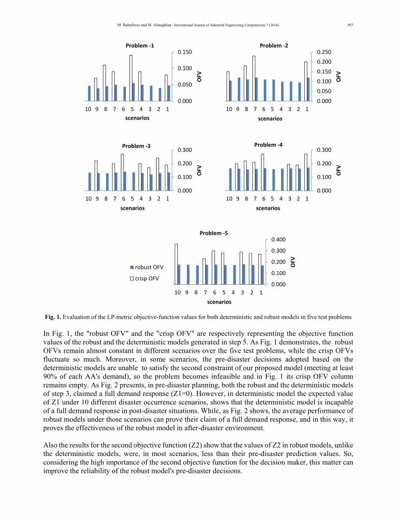
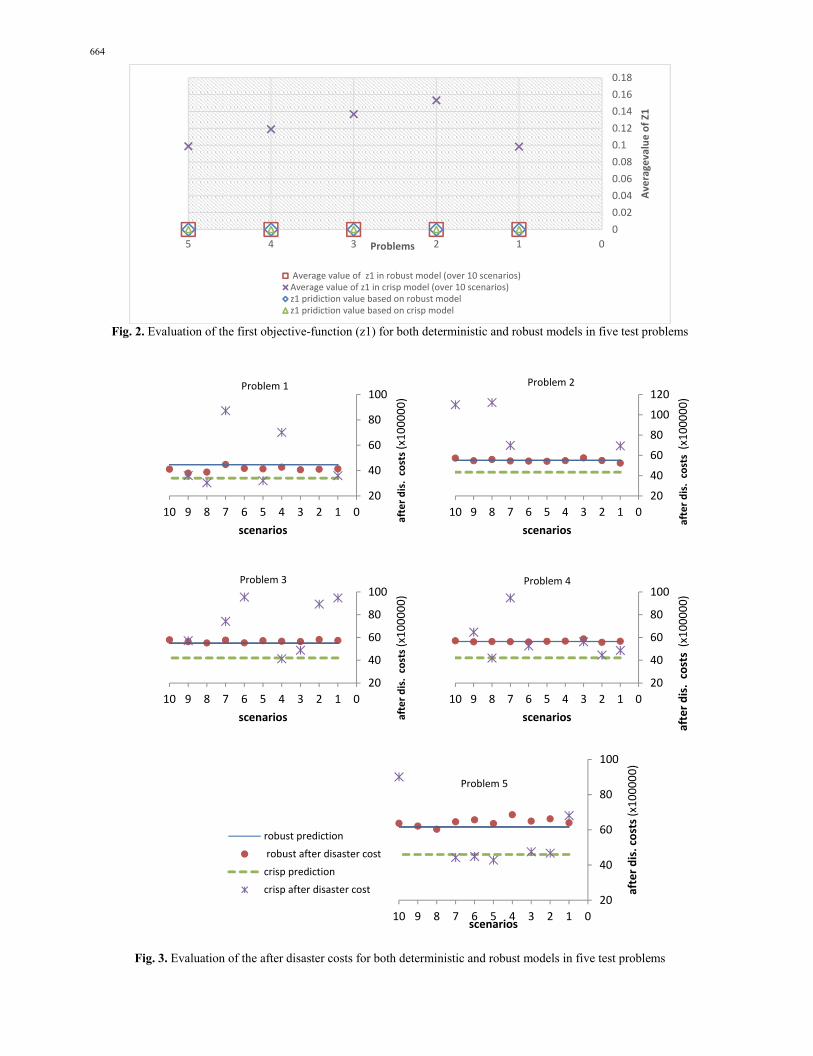
Fig. 1. Evaluation of the LP-metric objective-function values for both deterministic and robust models in five test problems In Fig. 1, the "robust OFV" and the "crisp OFV" are respectively representing the objective function values of the robust and the deterministic models generated in step 5. As Fig. 1 demonstrates, the robust OFVs remain almost constant in different scenarios over the five test problems, while the crisp OFVs fluctuate so much. Moreover, in some scenarios, the pre-disaster decisions adopted based on the deterministic models are unable to satisfy the second constraint of our proposed model (meeting at least 90% of each AA's demand), so the problem becomes infeasible and in Fig. 1 its crisp OFV column remains empty. As Fig. 2 presents, in pre-disaster planning, both the robust and the deterministic models of step 3, claimed a full demand response (Z1=0). However, in deterministic model the expected value of Z1 under 10 different disaster occurrence scenarios, shows that the deterministic model is incapable of a full demand response in post-disaster situations. While, as Fig. 2 shows, the average performance of robust models under those scenarios can prove their claim of a full demand response, and in this way, it proves the effectiveness of the robust model in after-disaster environment. Also the results for the second objective function (Z2) show that the values of Z2 in robust models, unlike the deterministic models, were, in most scenarios, less than their pre-disaster prediction values. So, considering the high importance of the second objective function for the decision maker, this matter can improve the reliability of the robust model's pre-disaster decisions.

0.000

0.050

0.100

0.150

0.200

0.250

12345678910

OFV

scenarios

Problem ‐2

0.000

0.050

0.100

0.150

12345678910

OFV

scenarios

Problem ‐1

0.000

0.100

0.200

0.300

12345678910

OFV

scenarios

Problem ‐4

0.000

0.100

0.200

0.300

12345678910OFV

scenarios

Problem ‐3

0.000

0.100

0.200

0.300

0.400

12345678910OFV

scenarios

Problem ‐5

robust OFV

crisp OFV

664

Fig. 2. Evaluation of the first objective-function (z1) for both deterministic and robust models in five test problems

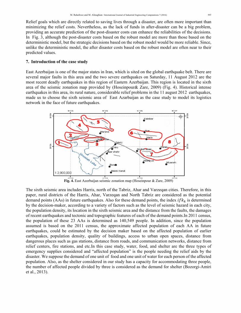
Fig. 3. Evaluation of the after disaster costs for both deterministic and robust models in five test problems

0

0.02

0.04

0.06

0.08

0.1

0.12

0.14

0.16

0.18

012345

Averagevalue of Z1

Problems

Average value of z1 in robust model (over 10 scenarios)Average value of z1 in crisp model (over 10 scenarios)z1 pridiction value based on robust modelz1 pridiction value based on crisp model

20

40

60

80

100

120

012345678910

after dis. costs (x100000)

scenarios

Problem 2

20

40

60

80

100

012345678910


scenarios

Problem 1

20

40

60

80

100

012345678910


scenarios

Problem 4

20

40

60

80

100

012345678910


scenarios

Problem 3

20

40

60

80

100

012345678910


scenarios

Problem 5

robust prediction

robust after disaster cost

crisp prediction

crisp after disaster cost


665

Relief goals which are directly related to saving lives through a disaster, are often more important than minimizing the relief costs. Nevertheless, as the lack of funds in after-disaster can be a big problem, providing an accurate prediction of the post-disaster costs can enhance the reliabilities of the decisions. In Fig. 3, although the post-disaster costs based on the robust model are more than those based on the deterministic model, but the strategic decisions based on the robust model would be more reliable. Since, unlike the deterministic model, the after disaster costs based on the robust model are often near to their predicted values.

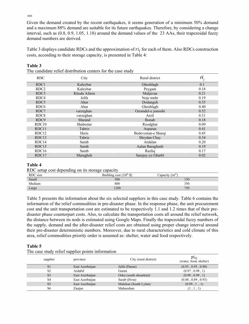
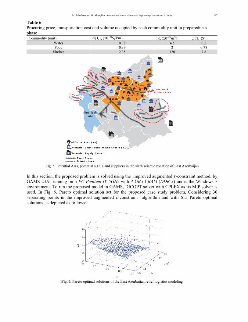
7. Introduction of the case study East Azerbaijan is one of the major states in Iran, which is sited on the global earthquake belt. There are several major faults in this area and the two severe earthquakes on Saturday, 11 August 2012 are the most recent deadly earthquakes in this region of Eastern Azerbaijan. This region is located in the sixth area of the seismic zonation map provided by (Hoseinpour& Zare, 2009) (Fig. 4). Historical intense earthquakes in this area, its rural nature, considerable relief problems in the 11 august 2012 earthquakes, made us to choose the sixth seismic area of East Azarbaijan as the case study to model its logistics network in the face of future earthquakes.

Fig. 4. East Azerbaijan seismic zonation map (Hoseinpour & Zare, 2009)

The sixth seismic area includes Harris, north of the Tabriz, Ahar and Varzeqan cities. Therefore, in this paper, rural districts of the Harris, Ahar, Varzeqan and North Tabriz are considered as the potential demand points (AAs) in future earthquakes. Also for these demand points, the index is determined by the decision-maker, according to a variety of factors such as the level of seismic hazard in each city, the population density, its location in the sixth seismic area and the distance from the faults, the damages of recent earthquakes and tectonic and topographic features of each of the demand points.In 2011 census, the population of these 23 AAs is determined as 140,549 people. In addition, since the population assumed is based on the 2011 census, the approximate affected population of each AA in future earthquakes, could be estimated by the decision maker based on the affected population of earlier earthquakes, population density, quality of buildings, access to urban open spaces, distance from dangerous places such as gas stations, distance from roads, and communication networks, distance from relief centers, fire stations, and etc.In this case study, water, food, and shelter are the three types of emergency supplies considered and “affected population” is the people needing the relief aids by the disaster. We suppose the demand of one unit of food and one unit of water for each person of the affected population. Also, as the shelter considered in our study has a capacity for accommodating three people, the number of affected people divided by three is considered as the demand for shelter (Bozorgi-Amiri et al., 2013).

666

Given the demand created by the recent earthquakes, it seems generation of a minimum 50% demand and a maximum 88% demand are suitable for its future earthquakes. Therefore, by considering a change interval, such as (0.8, 0.9, 1.05, 1.18) around the demand values of the 23 AAs, their trapezoidal fuzzy demand numbers are derived. Table 3 displays candidate RDCs and the approximation of for each of them. Also RDCs construction costs, according to their storage capacity, is presented in Table 4: Table 3 The candidate relief distribution centers for the case study

jri Rural district City RDC

0.1 Gheshlagh Kaleybar RDC1 0.18 Peygam Kaleybar RDC2 0.21MaljavanKhoda Afarin RDC3 0.19 Noje mehr Jolfa RDC4 0.35 Dodangeh Ahar RDC5 0.40GheshlaghAhar RDC6 0.52 Ozomdel-e jonoobi varzeghan RDC7 0.31 Arzil varzeghan RDC8 0.18 Bonab Marand RDC9 0.09 Roodghat Shabestar RDC10 0.41 Asparan Tabriz RDC11 0.45 Bedevostan-e Sharqi Heris RDC12 0.34 Meydan Chay Tabriz RDC13 0.20 Ardalan Sarab RDC14 0.19 Aalan Baraghush Sarab RDC15 0.17 Razliq Sarab RDC16 0.02 Sarajuy-ye Gharbi Maragheh RDC17

Table 4 RDC setup cost depending on its storage capacity

Capacity Building cost 10 $ RDC size 150 500 Small 350 800 Medium 750 1200 Large

Table 5 presents the information about the six selected suppliers in this case study. Table 6 contains the information of the relief commodities in pre-disaster phase. In the response phase, the unit procurement cost and the unit transportation cost are estimated to be respectively 1.1 and 1.2 times that of their pre-disaster phase counterpart costs. Also, to calculate the transportation costs all around the relief network, the distance between its nods is estimated using Google Maps. Finally the trapezoidal fuzzy numbers of the supply, demand and the after-disaster relief costs are obtained using proper change interval around their pre-disaster deterministic numbers. Moreover, due to rural characteristics and cold climate of this area, relief commodities priority order is assumed as: shelter, water and food respectively. Table 5 The case study relief supplier points information

pi (water, food, shelter) City (rural district) province supplier

(0.93 , 0.95 , 0.98) Julfa (Daran) East Azerbaijan S1 (0.97 , 0.98 , 1) Garmi Ardabil S2 (0.98 , 0.99 , 1) Osku (south shourkat)) East Azerbaijan S3

(0.88 , 0.89 , 0.93) Sarab (Hvm) East Azerbaijan S4 (0.99 , 1 , 1) Malekan (South Lylan) East Azerbaijan S5

(1 , 1 , 1) Mahneshan Zanjan S6


667

Table 6 Procuring price, transportation cost and volume occupied by each commodity unit in preparedness phase

1 ($) (10 ij1 (10 $/ Commodity (unit) 0.2 4.5 0.78 Water 0.78 2 0.39 Food 7.8 120 2.35 Shelter

Fig. 5. Potential AAs, potential RDCs and suppliers in the sixth seismic zonation of East Azerbaijan

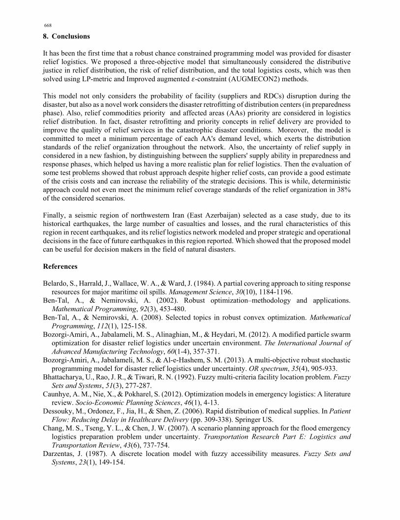
In this section, the proposed problem is solved using the improved augmented -constraint method, by GAMS 23.9 running on a PC Pentium IV-5GHz with 4 GB of RAM (DDR 3) under the Windows 7 environment. To run the proposed model in GAMS, DICOPT solver with CPLEX as its MIP solver is used. In Fig. 6, Pareto optimal solution set for the proposed case study problem, Considering 30 separating points in the improved augmented -constraint algorithm and with 615 Pareto optimal solutions, is depicted as follows:

Fig. 6. Pareto optimal solutions of the East Azerbaijan relief logistics modeling

668

8. Conclusions It has been the first time that a robust chance constrained programming model was provided for disaster relief logistics. We proposed a three-objective model that simultaneously considered the distributive justice in relief distribution, the risk of relief distribution, and the total logistics costs, which was then solved using LP-metric and Improved augmented -constraint (AUGMECON2) methods. This model not only considers the probability of facility (suppliers and RDCs) disruption during the disaster, but also as a novel work considers the disaster retrofitting of distribution centers (in preparedness phase). Also, relief commodities priority and affected areas (AAs) priority are considered in logistics relief distribution. In fact, disaster retrofitting and priority concepts in relief delivery are provided to improve the quality of relief services in the catastrophic disaster conditions. Moreover, the model is committed to meet a minimum percentage of each AA's demand level, which exerts the distribution standards of the relief organization throughout the network. Also, the uncertainty of relief supply in considered in a new fashion, by distinguishing between the suppliers' supply ability in preparedness and response phases, which helped us having a more realistic plan for relief logistics. Then the evaluation of some test problems showed that robust approach despite higher relief costs, can provide a good estimate of the crisis costs and can increase the reliability of the strategic decisions. This is while, deterministic approach could not even meet the minimum relief coverage standards of the relief organization in 38% of the considered scenarios. Finally, a seismic region of northwestern Iran (East Azerbaijan) selected as a case study, due to its historical earthquakes, the large number of casualties and losses, and the rural characteristics of this region in recent earthquakes, and its relief logistics network modeled and proper strategic and operational decisions in the face of future earthquakes in this region reported. Which showed that the proposed model can be useful for decision makers in the field of natural disasters. References Belardo, S., Harrald, J., Wallace, W. A., & Ward, J. (1984). A partial covering approach to siting response

resources for major maritime oil spills. Management Science, 30(10), 1184-1196. Ben-Tal, A., & Nemirovski, A. (2002). Robust optimization–methodology and applications.

Mathematical Programming, 92(3), 453-480. Ben-Tal, A., & Nemirovski, A. (2008). Selected topics in robust convex optimization. Mathematical

Programming, 112(1), 125-158. Bozorgi-Amiri, A., Jabalameli, M. S., Alinaghian, M., & Heydari, M. (2012). A modified particle swarm

optimization for disaster relief logistics under uncertain environment. The International Journal of Advanced Manufacturing Technology, 60(1-4), 357-371.

Bozorgi-Amiri, A., Jabalameli, M. S., & Al-e-Hashem, S. M. (2013). A multi-objective robust stochastic programming model for disaster relief logistics under uncertainty. OR spectrum, 35(4), 905-933.

Bhattacharya, U., Rao, J. R., & Tiwari, R. N. (1992). Fuzzy multi-criteria facility location problem. Fuzzy Sets and Systems, 51(3), 277-287.

Caunhye, A. M., Nie, X., & Pokharel, S. (2012). Optimization models in emergency logistics: A literature review. Socio-Economic Planning Sciences, 46(1), 4-13.

Dessouky, M., Ordonez, F., Jia, H., & Shen, Z. (2006). Rapid distribution of medical supplies. In Patient Flow: Reducing Delay in Healthcare Delivery (pp. 309-338). Springer US.

Chang, M. S., Tseng, Y. L., & Chen, J. W. (2007). A scenario planning approach for the flood emergency logistics preparation problem under uncertainty. Transportation Research Part E: Logistics and Transportation Review, 43(6), 737-754.

Darzentas, J. (1987). A discrete location model with fuzzy accessibility measures. Fuzzy Sets and Systems, 23(1), 149-154.


669

Dubois, D., & Prade, H. (1987). The mean value of a fuzzy number. Fuzzy sets and systems, 24(3), 279-300.

Duran, S., Gutierrez, M. A., & Keskinocak, P. (2011). Pre-positioning of emergency items for CARE international. Interfaces, 41(3), 223-237.

Haghani, A., & Afshar, A. (2009). Supply chain management in disaster response. Heilpern, S. (1992). The expected value of a fuzzy number. Fuzzy sets and Systems, 47(1), 81-86. Hoseinpour, M., & Zare, M. (2009). Seismic Hazard Assessment of Tabriz, a City in the Northwest of

Iran. Horner, M. W., & Downs, J. A. (2010). Optimizing hurricane disaster relief goods distribution: model

development and application with respect to planning strategies. Disasters, 34(3), 821-844. Inuiguchi, M., & Ramık, J. (2000). Possibilistic linear programming: a brief review of fuzzy

mathematical programming and a comparison with stochastic programming in portfolio selection problem. Fuzzy sets and systems, 111(1), 3-28.

Jia, H., Ordóñez, F., & Dessouky, M. (2007). A modeling framework for facility location of medical services for large-scale emergencies. IIE transactions, 39(1), 41-55.

Kongsomsaksakul, S., Yang, C., & Chen, A. (2005). Shelter location-allocation model for flood evacuation planning. Journal of the Eastern Asia Society for Transportation Studies, 6, 4237-4252.

Kovács, G., & Spens, K. M. (2007). Humanitarian logistics in disaster relief operations. International Journal of Physical Distribution & Logistics Management, 37(2), 99-114.

Luis, E., Dolinskaya, I. S., & Smilowitz, K. R. (2012). Disaster relief routing: Integrating research and practice. Socio-economic planning sciences, 46(1), 88-97.

Liu, B., & Iwamura, K. (1998). Chance constrained programming with fuzzy parameters. Fuzzy sets and systems, 94(2), 227-237.

Mavrotas, G. (2009). Effective implementation of the ε-constraint method in multi-objective mathematical programming problems. Applied mathematics and computation, 213(2), 455-465.

Mavrotas, G., & Florios, K. (2013). An improved version of the augmented ε-constraint method (AUGMECON2) for finding the exact pareto set in multi-objective integer programming problems. Applied Mathematics and Computation, 219(18), 9652-9669.

McCall, V. M. (2006). Designing and pre-positioning humanitarian assistance pack-up kits (HA PUKs) to support pacific fleet emergency relief operations. NAVAL POSTGRADUATE SCHOOL MONTEREY CA.

Mete, H. O., & Zabinsky, Z. B. (2010). Stochastic optimization of medical supply location and distribution in disaster management. International Journal of Production Economics, 126(1), 76-84.

Miettinen, K. (2012). Nonlinear multiobjective optimization (Vol. 12). Springer Science & Business Media.

Mulvey, J. M., Vanderbei, R. J., & Zenios, S. A. (1995). Robust optimization of large-scale systems. Operations research, 43(2), 264-281.

Najafi, M., Eshghi, K., & Dullaert, W. (2013). A multi-objective robust optimization model for logistics planning in the earthquake response phase. Transportation Research Part E: Logistics and Transportation Review, 49(1), 217-249.

Nolz, P. C., Doerner, K. F., Gutjahr, W. J., & Hartl, R. F. (2010). A bi-objective metaheuristic for disaster relief operation planning. In Advances in multi-objective nature inspired computing (pp. 167-187). Springer Berlin Heidelberg.

Owen, S. H., & Daskin, M. S. (1998). Strategic facility location: A review. European Journal of Operational Research, 111(3), 423-447.

Pishvaee, M. S., Razmi, J., & Torabi, S. A. (2012). Robust possibilistic programming for socially responsible supply chain network design: A new approach. Fuzzy sets and systems, 206, 1-20.

Psaraftis, H. N., Tharakan, G. G., & Ceder, A. (1986). Optimal response to oil spills: the strategic decision case. Operations Research, 34(2), 203-217.

Rao, J. R., & Saraswati, K. (1988). Facility location problem on a network under multiple criteria—fuzzy set theoretic approach.

670

Rawls, C. G., & Turnquist, M. A. (2010). Pre-positioning of emergency supplies for disaster response. Transportation research part B: Methodological, 44(4), 521-534.

Rubin, C. B., Saperstein, M. D., & Barbee, D. G. (1985). Community recovery from a major natural disaster.

Sherali, H. D., Carter, T. B., & Hobeika, A. G. (1991). A location-allocation model and algorithm for evacuation planning under hurricane/flood conditions. Transportation Research Part B: Methodological, 25(6), 439-452.

Soltani, R., Sadjadi, S. J., & Tavakkoli-Moghaddam, R. (2015). Entropy based redundancy allocation in series-parallel systems with choices of a redundancy strategy and component type: A multi-objective model. Appl. Math, 9(2), 1049-1058.

Steuer, R. E. (1986). Multiple criteria optimization: theory, computation, and applications. Wiley. Zhou, J., & Liu, B. (2007). Modeling capacitated location–allocation problem with fuzzy demands.

Computers & Industrial Engineering, 53(3), 454-468.

Documents

A novel robust chance constrained possibilistic