Embed Size (px)
Citation preview

A Numerical and Experimental Investigation
into Multi-Ionic Reactive Transport Behaviour in
Cementitious Materials
Brubeck Lee Freeman
Thesis submitted in candidature for the degree of Doctor of Philosophy at Cardiff University
2017

Acknowledgements
The research presented in this thesis would not have been possible without the financial support
of Cardiff University School of Engineering and the EPSRC, this is gratefully acknowledged.
Firstly I would like to thank my supervisors, Tony Jefferson and Peter Cleall, for providing me with
this opportunity and for your continuous help and guidance throughout the PhD. In particular I
would like to thank you for your understanding, support and encouragement during the difficult
times, without which I feel certain that I would not have made it to this point.
I would also like to thank my colleagues in offices W1.31 and W1.32, Stefani, Tom, Waled, Rob,
Martins, Chuansan, Monica, Toby, Olly, Adriana and Tharmesh for their help and advice and for
creating an enjoyable work environment.
In addition, I would like to thank the laboratory technical staff, Carl Wadsworth and Jack Morgan
for their assistance and guidance with the ion transport experiments.
I would like to thank my friends and family for all of their support and encouragement throughout.
I would particularly like to thank my wife Mitra, my mother and my mother-in-law for their
support and encouragement during the most difficult moments.
Finally I would like to specially thank all of my family, my mother, Kenny, my granddad, my
brothers and sisters and all of my in-laws for being amazing and for always being there for me no
matter what and Mitra for being the best partner I could have wished for.

Declaration
This work has not been submitted in substance for any other degree or award at this or any other university or place of learning, nor is being submitted concurrently in candidature for any degree or other award Signed ……………………………………………………… (candidate) Date ………………….…………….………
STATEMENT 1
This thesis is being submitted in partial fulfillment of the requirements for the degree of PhD
Signed ………………………………………….…………… (candidate) Date …………………………….……………
STATEMENT 2
This thesis is the result of my own independent work/investigation, except where otherwise
stated, and the thesis has not been edited by a third party beyond what is permitted by Cardiff
University’s Policy on the Use of Third Party Editors by Research Degree Students. Other sources
are acknowledged by explicit references. The views expressed are my own.
Signed ……………………………………….……….…… (candidate) Date …………………….…………………
STATEMENT 3
I hereby give consent for my thesis, if accepted, to be available online in the University’s Open
Access repository and for inter-library loan, and for the title and summary to be made available to
outside organisations.
Signed ……………………………………………..…..….. (candidate) Date …………………………………………

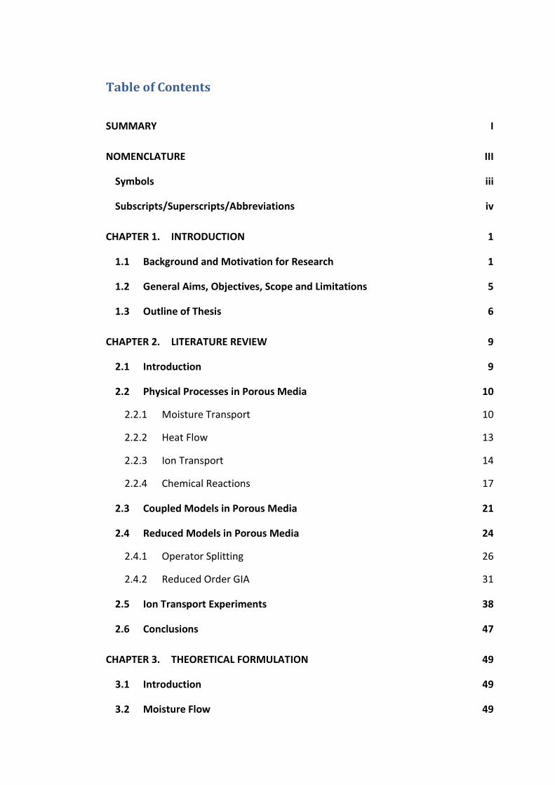
Table of Contents
SUMMARY I
NOMENCLATURE III
Symbols iii
Subscripts/Superscripts/Abbreviations iv
CHAPTER 1. INTRODUCTION 1
1.1 Background and Motivation for Research 1
1.2 General Aims, Objectives, Scope and Limitations 5
1.3 Outline of Thesis 6
CHAPTER 2. LITERATURE REVIEW 9
2.1 Introduction 9
2.2 Physical Processes in Porous Media 10
2.2.1 Moisture Transport 10
2.2.2 Heat Flow 13
2.2.3 Ion Transport 14
2.2.4 Chemical Reactions 17
2.3 Coupled Models in Porous Media 21
2.4 Reduced Models in Porous Media 24
2.4.1 Operator Splitting 26
2.4.2 Reduced Order GIA 31
2.5 Ion Transport Experiments 38
2.6 Conclusions 47
CHAPTER 3. THEORETICAL FORMULATION 49
3.1 Introduction 49
3.2 Moisture Flow 49
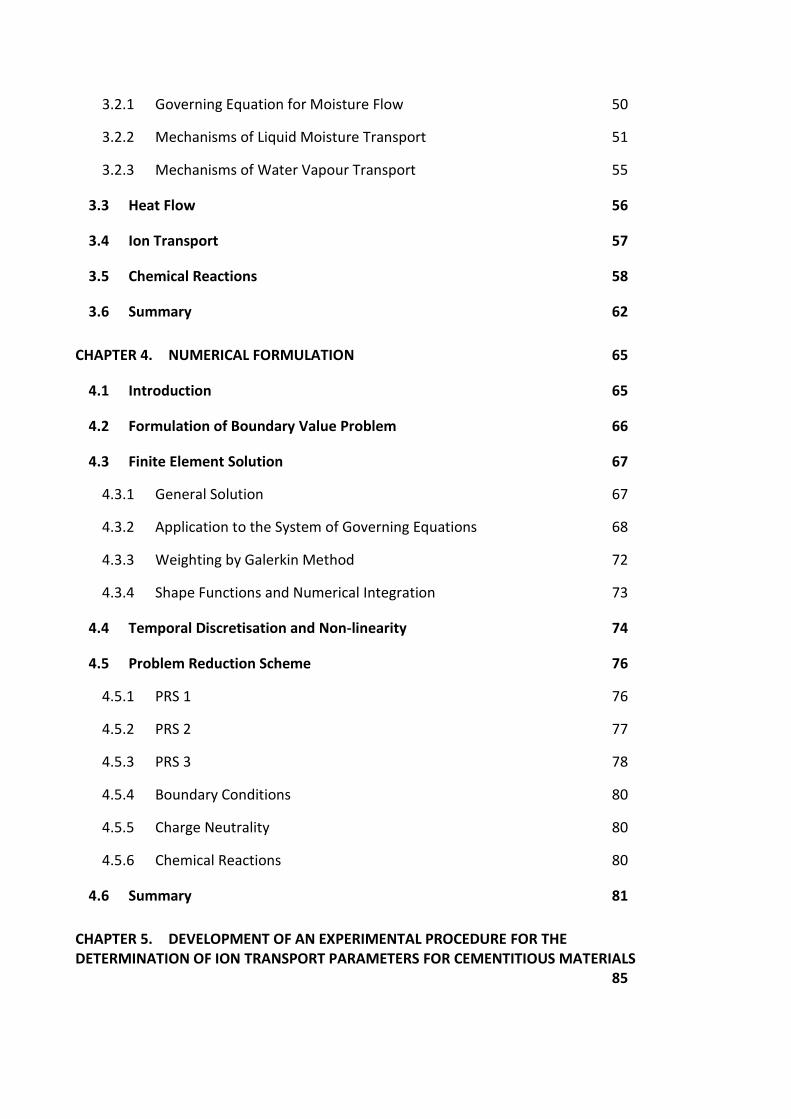
3.2.1 Governing Equation for Moisture Flow 50
3.2.2 Mechanisms of Liquid Moisture Transport 51
3.2.3 Mechanisms of Water Vapour Transport 55
3.3 Heat Flow 56
3.4 Ion Transport 57
3.5 Chemical Reactions 58
3.6 Summary 62
CHAPTER 4. NUMERICAL FORMULATION 65
4.1 Introduction 65
4.2 Formulation of Boundary Value Problem 66
4.3 Finite Element Solution 67
4.3.1 General Solution 67
4.3.2 Application to the System of Governing Equations 68
4.3.3 Weighting by Galerkin Method 72
4.3.4 Shape Functions and Numerical Integration 73
4.4 Temporal Discretisation and Non-linearity 74
4.5 Problem Reduction Scheme 76
4.5.1 PRS 1 76
4.5.2 PRS 2 77
4.5.3 PRS 3 78
4.5.4 Boundary Conditions 80
4.5.5 Charge Neutrality 80
4.5.6 Chemical Reactions 80
4.6 Summary 81
CHAPTER 5. DEVELOPMENT OF AN EXPERIMENTAL PROCEDURE FOR THE DETERMINATION OF ION TRANSPORT PARAMETERS FOR CEMENTITIOUS MATERIALS 85
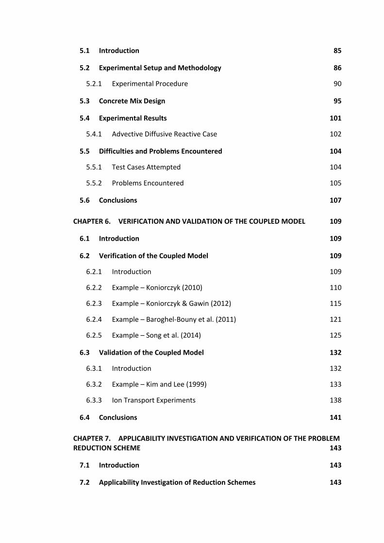
5.1 Introduction 85
5.2 Experimental Setup and Methodology 86
5.2.1 Experimental Procedure 90
5.3 Concrete Mix Design 95
5.4 Experimental Results 101
5.4.1 Advective Diffusive Reactive Case 102
5.5 Difficulties and Problems Encountered 104
5.5.1 Test Cases Attempted 104
5.5.2 Problems Encountered 105
5.6 Conclusions 107
CHAPTER 6. VERIFICATION AND VALIDATION OF THE COUPLED MODEL 109
6.1 Introduction 109
6.2 Verification of the Coupled Model 109
6.2.1 Introduction 109
6.2.2 Example – Koniorczyk (2010) 110
6.2.3 Example – Koniorczyk & Gawin (2012) 115
6.2.4 Example – Baroghel-Bouny et al. (2011) 121
6.2.5 Example – Song et al. (2014) 125
6.3 Validation of the Coupled Model 132
6.3.1 Introduction 132
6.3.2 Example – Kim and Lee (1999) 133
6.3.3 Ion Transport Experiments 138
6.4 Conclusions 141
CHAPTER 7. APPLICABILITY INVESTIGATION AND VERIFICATION OF THE PROBLEM REDUCTION SCHEME 143
7.1 Introduction 143
7.2 Applicability Investigation of Reduction Schemes 143
7.2.1 Results 147
7.2.2 Range of Applicability 164
7.2.3 Mass Balance 165
7.3 Verification of Reduction Schemes 166
7.3.1 PRS 1 – Baroghel-Bouny et al. (2011) 167
7.3.2 PRS 2 – Song et al. (2014) 171
7.3.3 PRS 3 – Hypothetical based on Zhu et al. (1999) 178
7.4 Computational Cost 193
7.5 Investigation into the use of Analytical Relationships for the Reduction Scheme 194
7.6 Conclusions 196
CHAPTER 8. CONCLUSIONS AND FUTURE WORK 199
REFERENCES 205
APPENDICES 217
A1 – Model Parameters 217
A2 – PRS Results 218
Calibration Problem 218
Verification Example 3 Results 235
i
Summary
This thesis describes a FE approach to the simulation of reactive transport problems
and a simple experimental procedure for the determination of transport parameters in
cementitious materials.
A comprehensive fully coupled reactive-thermo-hygro-chemical model was developed
based on the governing equations of mass and enthalpy balance. The model takes into
consideration advective-dispersive transport of solutes, heat flow, advective-diffusive
moisture flow, and chemical reactions. The FEM, Euler backward difference scheme
and Newton-Raphson iteration procedure were employed to solve the system of
nonlinear equations. To address the numerical challenge associated with such coupled
simulations, three problem reduction schemes were proposed, each of which uses a
reduced set of species, termed ‘indicators’, for full computation. The response of the
remaining species is computed at each time step from the transport of the indicators.
The difference between the schemes lies in the number of indicator species used and
in the method employed for calculating the transport of the remaining species.
Firstly the development of the experimental procedure is presented including the
design of a porous concrete mix, a discussion of the problems encountered and the
results of an advective-diffusive case. Following this, the model is validated and
verified against a number of problems, beginning with a moisture transport problem
and ending with a multi-ionic reactive transport problem. It was found that the model
was able to accurately capture the transport behaviour. The range of applicability of
each of the reduction schemes is then investigated through an example problem
concerning the reactive transport of 16 chemical species, before verifying each of the
schemes against the full model through the consideration of three example problems.
The reduction schemes were found to perform well in accurately capturing the
transport behaviour whilst greatly reducing the number of coupled equations to be
solved, and the computational cost of the simulation.

ii
iii
Nomenclature
Symbols
a1-5, ac Material parameters A1-3, Ak, Av, Aw, Aλ Material parameters
Debye-Hückel parameter A’, A’2 Reaction parameter acti Solution activity b, b1-5 Material parameters bp Universal parameter Bv Material parameter
Bma, Bmx, ,
Virial coefficients
ci Concentration of species i C Global secant matrix Ci Specific heat of phase i
Cma, Cmx, Virial coefficients
Dij j diffusion/dispersion of type i fi Global body force vector of phase i fs Material parameter f(T), Fϕ Pitzer functions F Faraday’s constant g Gravity vector g(x), g’(x) Pitzer functions Hci Heat of reaction i Hv Heat of vaporisation I Ionic strength of solution Jij j flux of type i ka, kd, kda Reaction rate parameters kt Thermal conductivity K Global mass matrix Ki Permeability of type i Keq Equilibrium constant of reaction mij j mass of type i Mi Molecular mass of type i n Unit normal vector ni Porosity of type i N Shape function matrix Number of degrees of freedom nelem Number of elements nr Number of reactions ns Number of species Pi Pressure of phase i qi Flux of phase i q1-6 Pitzer parameters R Molar gas constant S Solution Supersaturation ratio Si Degree of saturation of phase i

iv
Subscripts/Superscripts/Abbreviations 0 Initial atm Atmospheric c Cauchy C Capillary d Dispersive da Dry air di Dirichlet diff Diffusive e Element env Environment es Electrostatic double layer g Gas ind Indicator
t Time Tcc Total chloride content
T Temperature Tr Reference temperature vi Velocity of type i vi Valence of type i W Weighting function zi Charge of species i Z Charge function , Virial coefficient parameters Boundary mass transfer coefficient , Longitudinal and transverse dispersivities Boundary mass transfer coefficient
, ,
Virial coefficient parameters
Boundary mass transfer coefficient , Activity coefficient of an anion and cation Problem boundary
Kronecker delta
Dielectric permittivity λ Order of reaction
Viscosity of phase i Free surface energy Charge density Density of phase i Mass averaged density of phase i
Heat capacity τ Tortuosity Residual from approximation Osmotic coefficient Vector of primary variables Electric potential Problem domain

v
ind,l Lower indicator ind,m Middle indicator ind,u Upper indicator i Intrinsic k Iteration m Anion mol Molecular mv Moisture vapour p Precipitated/sorbed PRS Problem reduction scheme q Heat r Reference rg Relative gas RH Relative humidity rw Relative water s Solid t Time qi Boundary flux i v Vapour vs Vapour saturated w Water x Cation Γ Boundary

1
Chapter 1. Introduction
1.1 Background and Motivation for Research
The prediction of thermo, hygro, and chemical transport behaviour in porous materials
is of great importance in a wide range of engineering applications. To this end, a large
number of analytical and numerical transport models have been developed. Typically
these are coupled models which consider the advective-dispersive transport of a
solute, heat flow, the advective-diffusive moisture flow, and often mechanical
behaviour of the medium. In addition to these flow and deformation processes, the
solute can be considered as reactive or non-reactive, depending on the application.
These models have existed for a number of decades, with a number of reactive models
having been developed in the 1970’s and 80’s (Rubin and James 1973; Valocchi et al.
1981; Rubin 1983; Lichtner 1985). The application of these models has varied
considerably, with much of the previous work concentrating on geochemical problems
such as modelling groundwater systems (Yeh and Tripathi 1991; Walter et al. 1994;
Parkhurst and Wissmeier 2015), assessing the performance of engineered barriers
(Gens et al. 2004; Cleall et al. 2007; Thomas et al. 2012), or attenuation of mine water
tailings (Zhu et al. 1999; Bertocchi et al. 2006). The application of these models to
cementitious materials has most often investigated the ingress of chloride ions (Song
et al. 2008; Baroghel-Bouny et al. 2009; Koniorczyk and Gawin 2012), or calcium
leaching (Kuhl et al. 2004; Gawin et al. 2009). However, recently these models have
also been used for investigating self-healing concrete (Aliko-Benítez et al. 2015; Chitez
and Jefferson 2016).
The problem with these types of models is that the computational demand can be very
high, depending on the chemical system. Cleall et al. (2006) suggest that this is
governed by the following three main aspects of a problem:
1. Domain size, which affects not only the memory storage required but also the
computational cost of solving large sets of simultaneous equations.

2
2. Timescale, which affects the number of times that this set of simultaneous
equations need to be solved, and which for geochemical problems can be many
years, with a fine resolution required to accurately capture the behaviour.
3. Complexity of the analysis, which can be split into four factors:
a. The number of variables (affecting memory storage requirements and
the computational cost of solving large sets of simultaneous equations).
b. Degree of coupling between the variables, i.e. if the chemicals are
involved in many reactions with one another (affecting whether a fully
coupled solution is required).
c. Non-linearity of the system (affecting the number of times the set of
simultaneous equations need to be solved in one time step).
d. The number of processes considered.
An example of this high computational demand can be seen in the hypothetical Tokyo
bay case study, modelled by Yamamoto et al. (2009; 2014). This case study was of the
geological storage of CO2 in a 60×70 km area centred in Tokyo Bay. The authors used
an efficient parallel simulator TOUGH2-MP/ECO2N (Zhang et al. 2007) and ran the
simulations on the Earth Simulator (ES) supercomputer which consists of a total of
5120 processors and 10 TB memory. The domain was discretised into 10 million grid
cells, with 3 degrees of freedom per node for the multi-phase flow problem, leading to
a total of 30 million degrees of freedom. The time period considered was 1000 years
and the authors found that the simulations generally took 1-2 days.
The high computational demand is commonly dealt with in one of two ways in the
literature. The first, termed ‘operator splitting’, separates the calculation of the
transport and the chemical reactions in a time step, effectively decoupling the
chemical transport equations from the reaction equations, with a number of models
then iterating between the two. The chemical reaction equations, however, may still
be coupled in this approach. In addition to this, the splitting of the calculations has
been found to introduce mass balance errors for certain boundary conditions (Valocchi
and Malmstead 1992) and the iterative methods may require a prohibitively small time
step or large number of iterations to converge (Hoffmann et al. 2012). The second
approach is to reformulate the system of equations, using the problem stoichiometry,
3
and introduce transformed variables. The aim is to decouple a number of the transport
equations and eliminate some local (spatially invariant) equations. The amount of
reduction that can be achieved is often limited by the problem chemistry (for example
if there are a large number of kinetic reactions considered). Many also impose the
assumption of equal diffusion coefficients for all species, which has been found to be
inaccurate for certain chemical systems (Thomas et al. 2012). One of the aspects of this
study is to consider the development of methods which allows a greater reduction of
problem size, whilst also allowing for species dependent diffusion coefficients.
In order to predict the transport behaviour, these models rely on a number of
parameters that need to be determined experimentally. These include the
permeability and conductivity of the medium, the ion diffusion and dispersion
coefficients, and the chemical reaction parameters, including the order and rate of the
reactions. These issues have been investigated experimentally for soil leaching
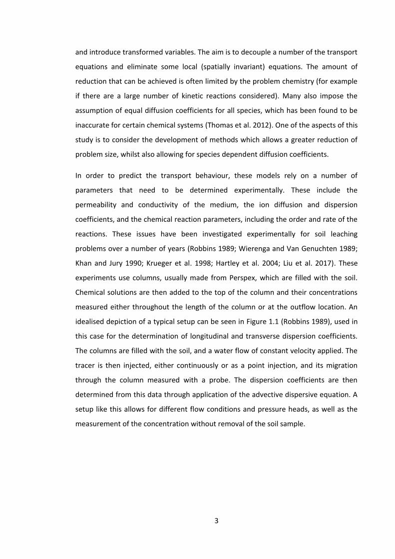
problems over a number of years (Robbins 1989; Wierenga and Van Genuchten 1989;
Khan and Jury 1990; Krueger et al. 1998; Hartley et al. 2004; Liu et al. 2017). These
experiments use columns, usually made from Perspex, which are filled with the soil.
Chemical solutions are then added to the top of the column and their concentrations
measured either throughout the length of the column or at the outflow location. An
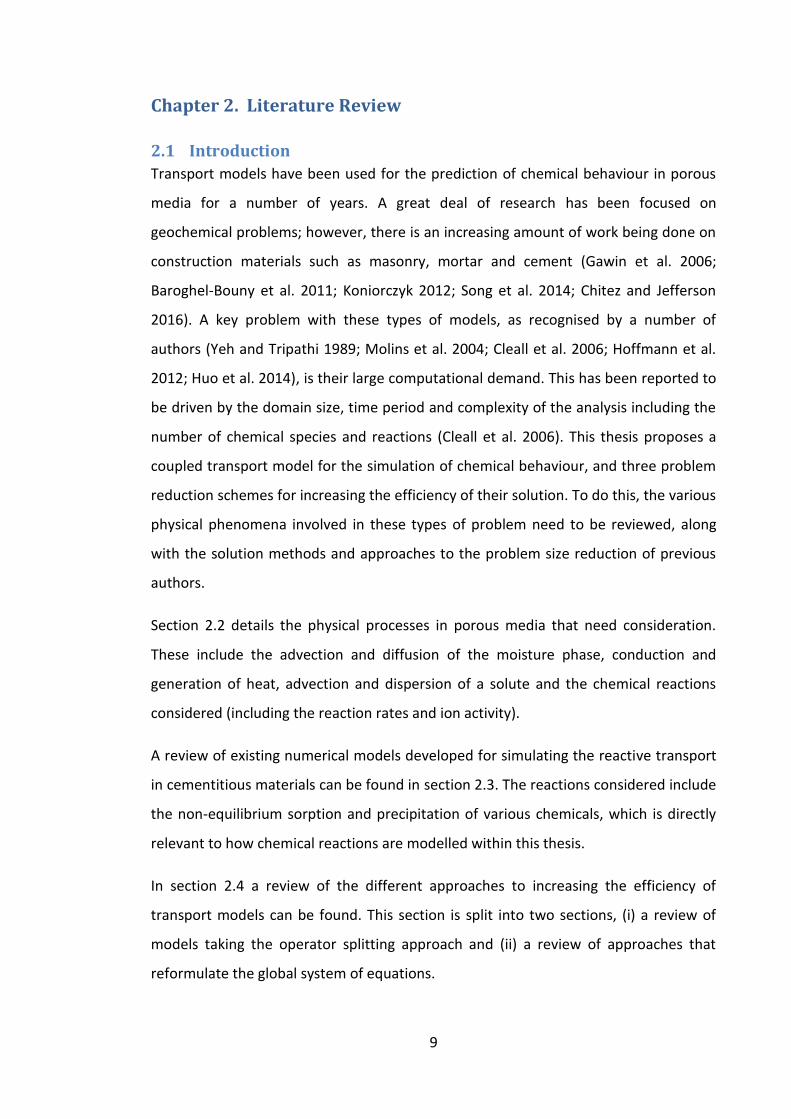
idealised depiction of a typical setup can be seen in Figure 1.1 (Robbins 1989), used in
this case for the determination of longitudinal and transverse dispersion coefficients.
The columns are filled with the soil, and a water flow of constant velocity applied. The
tracer is then injected, either continuously or as a point injection, and its migration
through the column measured with a probe. The dispersion coefficients are then
determined from this data through application of the advective dispersive equation. A
setup like this allows for different flow conditions and pressure heads, as well as the
measurement of the concentration without removal of the soil sample.
4
Figure 1.1 – Idealised column set up for a) Continuous injection and b) Point injection (after Robbins (1989))
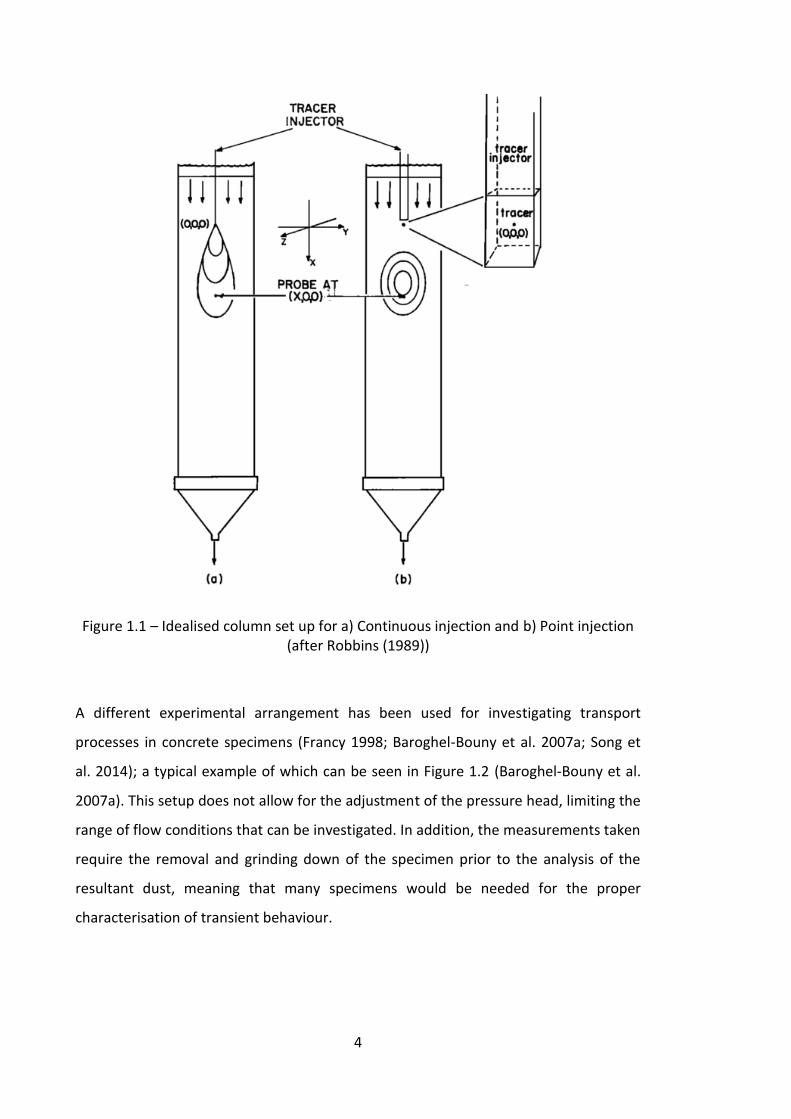
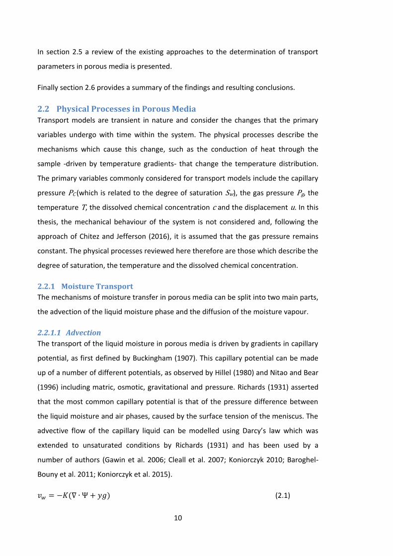
A different experimental arrangement has been used for investigating transport
processes in concrete specimens (Francy 1998; Baroghel-Bouny et al. 2007a; Song et
al. 2014); a typical example of which can be seen in Figure 1.2 (Baroghel-Bouny et al.
2007a). This setup does not allow for the adjustment of the pressure head, limiting the
range of flow conditions that can be investigated. In addition, the measurements taken
require the removal and grinding down of the specimen prior to the analysis of the
resultant dust, meaning that many specimens would be needed for the proper
characterisation of transient behaviour.
5
Figure 1.2 – Diffusion/wetting test setup (after Baroghel-Bouny et al. (2007))
Another aspect of this study is to consider the development of a simple ion transport
experimental procedure for cementitious materials, which allows the application of
different pressure heads, and allows the measurement of the concentration profile
without the removal of the specimen, making it simpler to investigate the transient
chemical behaviour.
1.2 General Aims, Objectives, Scope and Limitations
The work of this thesis had two main aims which are as follows:
1. Develop a numerical approach to enable problem size reduction that would
reduce the computational demand associated with the simulation of reactive
transport problems.
2. Develop an experimental test procedure for the investigation of transport
behaviour in cementitious materials, which allows for different flow conditions
and the measurement of transient behaviour, without requiring the removal of
the specimen from the test setup.
These will be met by satisfaction of the following detailed objectives:
1. Develop a coupled model based on a reliable mathematical framework for the
simulation of reactive transport problems in porous media.
2. Investigate the behaviour of the coupled model for different chemical systems,
including different boundary conditions, a range of transport behaviour and
various reactions to determine the validity of the model.

6
3. Propose a problem reduction scheme for use in complex multi-ionic systems in
order to reduce the computational cost of the simulations.
4. Investigate the problem reduction scheme to determine the range of
applicability of each of the approaches, before investigating the behaviour of
the schemes for different chemical systems including different boundary
conditions, a range of transport behaviour and various reactions to determine
the validity of the approach.
5. Develop a simple alternative to column leaching tests for cementitious
materials using lab scale concrete beams and carry out tests in order to
determine different chemical parameters such as dispersion coefficients, as
well as providing data for the validation of the proposed model.
The scope and limitations of this study are as follows:
1. It is assumed that the domain is isotropic.
2. The reactions considered throughout are kinetic, such that chemical
equilibrium conditions are not assumed.
3. No investigation is made into temperature changes, including warming/cooling
of the medium and the enthalpy change of chemical reactions.
4. Diffusion coefficients are considered to be constant irrespective of chemical
concentrations and moisture content.
5. The chemical activity of the pore water is assumed to have no effect on the
transport of ions or moisture.
6. Gas pressure changes are assumed to be negligible such that they are
neglected in the model.
7. The chemical concentration is assumed to have no effect on the moisture
retention characteristics of the medium.
8. The porous matrix is assumed to be rigid.
1.3 Outline of Thesis
This thesis is divided into 8 chapters and 1 appendix. Chapter 2 provides a review of
the literature including an overview of the theory behind the physical processes and
chemical reactions that are used for simulating the chemical behaviour in porous
7
media. A review of current models that have been developed by other authors is
presented, with particular attention being directed towards current approaches to
problem size reduction. Finally, a brief overview of current ion transport experimental
procedures used for both soils and cementitious materials is given.
Chapter 3 details the theoretical formulations required for the development of a
coupled transport model, including the description of chemical reactions and ion
activity.
Chapter 4 details the numerical formulation and the application of the finite element
method to the governing equations derived in Chapter 3. Both the spatial and
temporal discretisation are discussed, as well as the iteration procedure employed to
deal with the problem non-linearity. The chapter ends with the proposal and
description of a series of problem reduction schemes.
The development of an experimental procedure for chemical transport in cementitious
materials is presented in Chapter 5 beginning with a description of the methodology,
and concluding with results and a description of the problems encountered during the
investigation.
The verification and validation of the full coupled model is detailed in Chapter 6. The
model is first verified against numerical results found in the literature, before being
validated against drying experiments and the results of the experiments presented in
the previous chapter.
In Chapter 7 the behaviour of the proposed problem reduction schemes will be
investigated. This begins with an investigation into the range of validity of each of the
methods through the consideration of a 16 ion reactive transport problem. Following
this, each of the three reduction schemes are verified through comparison with the full
model on the simulation of three example problems.
Finally, Chapter 8 gives the general conclusions of the thesis and provides suggestions
for future research.

8
9
Chapter 2. Literature Review
2.1 Introduction
Transport models have been used for the prediction of chemical behaviour in porous
media for a number of years. A great deal of research has been focused on
geochemical problems; however, there is an increasing amount of work being done on
construction materials such as masonry, mortar and cement (Gawin et al. 2006;
Baroghel-Bouny et al. 2011; Koniorczyk 2012; Song et al. 2014; Chitez and Jefferson
2016). A key problem with these types of models, as recognised by a number of
authors (Yeh and Tripathi 1989; Molins et al. 2004; Cleall et al. 2006; Hoffmann et al.
2012; Huo et al. 2014), is their large computational demand. This has been reported to
be driven by the domain size, time period and complexity of the analysis including the
number of chemical species and reactions (Cleall et al. 2006). This thesis proposes a
coupled transport model for the simulation of chemical behaviour, and three problem
reduction schemes for increasing the efficiency of their solution. To do this, the various
physical phenomena involved in these types of problem need to be reviewed, along
with the solution methods and approaches to the problem size reduction of previous
authors.
Section 2.2 details the physical processes in porous media that need consideration.
These include the advection and diffusion of the moisture phase, conduction and
generation of heat, advection and dispersion of a solute and the chemical reactions
considered (including the reaction rates and ion activity).
A review of existing numerical models developed for simulating the reactive transport
in cementitious materials can be found in section 2.3. The reactions considered include
the non-equilibrium sorption and precipitation of various chemicals, which is directly
relevant to how chemical reactions are modelled within this thesis.
In section 2.4 a review of the different approaches to increasing the efficiency of
transport models can be found. This section is split into two sections, (i) a review of
models taking the operator splitting approach and (ii) a review of approaches that
reformulate the global system of equations.
10
In section 2.5 a review of the existing approaches to the determination of transport
parameters in porous media is presented.
Finally section 2.6 provides a summary of the findings and resulting conclusions.
2.2 Physical Processes in Porous Media
Transport models are transient in nature and consider the changes that the primary
variables undergo with time within the system. The physical processes describe the
mechanisms which cause this change, such as the conduction of heat through the
sample -driven by temperature gradients- that change the temperature distribution.
The primary variables commonly considered for transport models include the capillary
pressure PC (which is related to the degree of saturation Sw), the gas pressure Pg, the
temperature T, the dissolved chemical concentration c and the displacement u. In this
thesis, the mechanical behaviour of the system is not considered and, following the
approach of Chitez and Jefferson (2016), it is assumed that the gas pressure remains
constant. The physical processes reviewed here therefore are those which describe the
degree of saturation, the temperature and the dissolved chemical concentration.
2.2.1 Moisture Transport
The mechanisms of moisture transfer in porous media can be split into two main parts,
the advection of the liquid moisture phase and the diffusion of the moisture vapour.
2.2.1.1 Advection
The transport of the liquid moisture in porous media is driven by gradients in capillary
potential, as first defined by Buckingham (1907). This capillary potential can be made
up of a number of different potentials, as observed by Hillel (1980) and Nitao and Bear
(1996) including matric, osmotic, gravitational and pressure. Richards (1931) asserted
that the most common capillary potential is that of the pressure difference between
the liquid moisture and air phases, caused by the surface tension of the meniscus. The
advective flow of the capillary liquid can be modelled using Darcy’s law which was
extended to unsaturated conditions by Richards (1931) and has been used by a
number of authors (Gawin et al. 2006; Cleall et al. 2007; Koniorczyk 2010; Baroghel-
Bouny et al. 2011; Koniorczyk et al. 2015).
( ) (2.1)
11
where is the liquid velocity, K is the conductivity or coefficient of permeability, y is
the height above a datum, is the acceleration due to gravity and is the capillary
potential. It should be noted, however, that this equation describes the flow of the
capillary liquid, which is the liquid that is not adsorbed to the solid matrix (Richards
1931). For liquid moisture coming into a dry medium, the initial liquid transport is
driven by adhesive forces between the molecules until the solid is wetted, covering the
solid in a thin film (pendular state); it is after this that liquid transport due to other
forces can take place (funicular state). It can be said then that eq. (2.1) is only valid for
moisture in the funicular state, and therefore there is no moisture transport below a
particular value of saturation (which describes the adsorbed water content). In
investigating heat and moisture transport at high temperature in cementitious
materials, Davie et al. (2006) found that ignoring the adsorbed water content can have
a significant effect on the prediction of moisture fluxes, vapour contents and gas
pressures.
The coefficient of permeability in eq. (2.1) is dependent on a number of different
variables including porosity, damage, degree of saturation and temperature and has a
wide range of values for porous media ranging from 10-9 m2 for clean sand (Bear and
Verruijt 1987) to 10-21 m2 (or lower) for cementitious materials (Baroghel-Bouny et al.
2011; Koniorczyk et al. 2015). The effective permeability therefore can be given by the
multiple of the intrinsic permeability Ki (which is dependent on the medium) and the
relative permeability Krw as follows:
(2.2)
where the relative permeability takes into account the effects of the aforementioned
variables. For the dependence of the relative permeability on the degree of saturation,
there are two schools of thought (Mualem 1976), the first being that the relative
permeability is a power function of the degree of saturation. An expression of this first
type has been derived analytically by Irmay (1954), who found that a cubic function
was appropriate. This approach has been adopted by a number of authors (Gawin et
al. 1999; Cleall et al. 2007; Koniorczyk and Gawin 2011). The second group derive
analytical expressions for the relative permeability based on the moisture retention
12
curve for a given medium. Examples of such approaches can be found in (Brooks and
Corey 1964; Mualem 1976; van Genuchten 1980); which have also been used by a
number of authors (Koniorczyk 2010; Baroghel-Bouny et al. 2011; Koniorczyk 2012).
The moisture vapour advection can also be described using the eq. (2.1); however,
according to Chitez and Jefferson (2016), the gas pressure quickly reaches steady state
and so therefore this is neglected.
2.2.1.2 Retention
It was mentioned in the previous section that the capillary potential (or capillary
pressure) mainly arose as a result of the pressure difference between the liquid
moisture and air phases. The magnitude of this pressure depends on both the surface
tension and the curvature of the separating meniscus which in turn depends on the
moisture content of the medium (Bear and Verruijt 1987). There is a relationship then
between the capillary pressure and the moisture content of the medium, which is
dependent on the pore structure of the medium (Richards 1931; Bear and Verruijt
1987; Baroghel-Bouny et al. 2011). In initial work undertaken by Buckingham (1907),
measurements were made of the soil-moisture retention curves for various types of
soil. In his classic paper, van Genuchten (1980) proposed an analytical relationship
between the two, using just two fitting parameters to take into account different pore
structures. This relationship is given by:
(
)
(2.3)
where PC is the capillary pressure, Sw is the degree of liquid saturation and a and m are
material parameters. Some authors have also included the effects of chemical
concentration or temperature on this retention curve. For example, Koniorczyk and
Wojciechowski (2009) used neural networks to model the influence of salt
concentration on this retention curve and found that at high saturations (or high salt
content) these effects can be significant. By contrast, Baroghel-Bouny et al. (2011)
found that for the cement mortars, at the concentrations and degrees of hydration
considered, these effects (temperature and chemical concentration) had a negligible
influence on the retention curve parameters. For the temperature dependence, Cleall
13
(1998) describes an approach following work by Edlefsen and Anderson (1943) and
Fredlund and Rahardjo (1993) in which the capillary pressure can be related to the free
surface energy which is a function of temperature; stating that the relative change in
free surface energy with temperature is equal to the relative change in capillary
pressure.
2.2.1.3 Diffusion
The diffusion of moisture vapour within a porous medium is caused by molecular
diffusion and as such is assumed to be governed by Fick’s law (Philip and De Vries
1957; Gawin et al. 2006):
(2.4)
where Jv is the vapour flux, Dm is the moisture vapour diffusivity and ρv is the density of
the moisture vapour phase. Tie-hang and Li-jun (2009) state that the transfer of
moisture vapour is driven by both capillary pressure and temperature gradients. The
effect of temperature gradients was discussed in detail in the classic paper by Philip
and De Vries (1957) who also noted that, at low moisture contents, transport via
diffusion was dominant. Gawin et al. (1999) reports that, like the permeability, the
vapour diffusion through a porous medium is also dependent on the properties of that
medium; including the porosity, degree of saturation and tortuosity (Knudsen effect).
2.2.2 Heat Flow
2.2.2.1 Conduction
The behaviour of heat transport in porous media has been subject to a great deal of
investigation. These investigations range from heat loss from ground source heat
transfer (Rees et al. 2000) to the heat of hydration of cementitious materials (De
Schutter and Taerwe 1995). Gawin et al. (2011a; 2011b) studied the effects of high
temperature on concrete structures in order to determine the effect of the different
heat phenomena, concluding that convective heat transfer could be ignored with little
loss of model accuracy. The conduction of heat is assumed to follow Fourier’s law and
is given as (Gawin et al. 2006):
(2.5)
14
where Jq is the heat flux, kt is the thermal conductivity and T is the temperature. The
thermal conductivity is reported to depend on the temperature, moisture content and
porosity of the medium (Gawin et al. 1999).
2.2.2.2 Heat Generation
Another key consideration in the heat behaviour of a porous medium is the heat
generation; this can be heat change from external sources or heat change due to
chemical reactions. The heat change due to a chemical reaction is caused by the
change in enthalpy in a system caused by the chemical reaction. For example, if we
consider the formation of NaCl:
( )
( ) ( ), (2.6)
where is the enthalpy of the reaction and a negative value indicates that this is an
exothermic reaction, meaning that heat is released. The effects of this enthalpy change
has been included in the models of a number of authors (De Schutter and Taerwe
1995; Gawin et al. 2006; Gawin et al. 2009; Thomas et al. 2009; Koniorczyk 2010;
Koniorczyk 2012). De Schutter and Taerwe (1995) considered the heat generated from
the hydration reaction of Portland cement and blast furnace slag cement; predicting
the heat generation rate based on the temperature and degree of hydration.
Koniorczyk (2010; 2012) included in his model the heat generated from precipitation of
salt in cement mortar and bricks and suggested that integration of the temperature
profiles compared with pure water profiles, could serve as an indication of the amount
of precipitated salt within the system. The change in temperature caused by reactions
can also induce pore water movement due to the temperature gradients; this was
taken into account by Thomas et al. (2009), who considered the cryogenic suction
caused by the interface between ice and water in permafrost and frozen soils.
2.2.3 Ion Transport
The transport of chemical ions in pore water is split into two parts, the advection
caused by the movement of the pore water and the hydrodynamic dispersion which
accounts for the movement of ions within the pore water.
15
2.2.3.1 Advection
The advection of dissolved chemical ions is due to the pore water velocity and
therefore the physical processes that govern this behaviour have been described in
section 2.2.1.1. There are, however, some differences which may arise as a result of
the presence of the ions. The most widely considered is the effect of the chemical
concentration on the viscosity of the pore liquid which has been included in the
models of a number of authors (Koniorczyk and Wojciechowski 2009; Baroghel-Bouny
et al. 2011). Some authors take things further and include the flow of pore water due
to chemical concentration gradients, known as osmotic flow (Cleall et al. 2007).
2.2.3.2 Hydrodynamic Dispersion
The next key transport process of dissolved chemical ions is the hydrodynamic
dispersion. This is considered in two key ways, the first is a multi-species model which
takes into account the differential molecular diffusion coefficients of each species
allowing for different rates of transport for each ion (Samson and Marchand 2007;
Baroghel-Bouny et al. 2011; Song et al. 2014). The second assumes that all species
have the same diffusion coefficient and so the rate of transport is equal for all ions
(Zhu et al. 1999; Cleall et al. 2007; Hoffmann et al. 2012). The justification for the
second approach is that in the system under consideration the molecular diffusion
coefficient is small in comparison to the mechanical dispersion (Zhu et al. 1999; Kräutle
and Knabner 2007; Hoffmann et al. 2012). The hydrodynamic dispersion is composed
of two different phenomena, the molecular diffusion, which is the spreading of the
ions due to their random movement in the pore water and the mechanical dispersion
(Bear and Verruijt 1987). The mechanical dispersion is the spreading of the ions due to
the pore water flow; this is split into two parts, the spreading of the pore water as it
flows around solid particles, and the spreading due to the velocity distribution within
the pores. The effects of these phenomena can be seen in Figure 2.1.
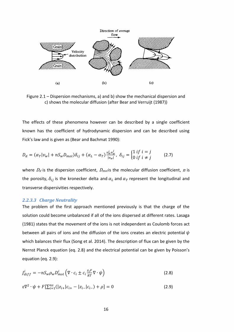
16
Figure 2.1 – Dispersion mechanisms, a) and b) show the mechanical dispersion and c) shows the molecular diffusion (after Bear and Verruijt (1987))
The effects of these phenomena however can be described by a single coefficient
known has the coefficient of hydrodynamic dispersion and can be described using
Fick’s law and is given as (Bear and Bachmat 1990):
( | | ) ( )
| |, {
(2.7)
where Dd is the dispersion coefficient, Dmol is the molecular diffusion coefficient, n is
the porosity, is the kronecker delta and and represent the longitudinal and
transverse dispersivities respectively.
2.2.3.3 Charge Neutrality
The problem of the first approach mentioned previously is that the charge of the
solution could become unbalanced if all of the ions dispersed at different rates. Lasaga
(1981) states that the movement of the ions is not independent as Coulomb forces act
between all pairs of ions and the diffusion of the ions creates an electric potential
which balances their flux (Song et al. 2014). The description of flux can be given by the
Nernst Planck equation (eq. 2.8) and the electrical potential can be given by Poisson’s
equation (eq. 2.9):
(
) (2.8)
[∑ (| | | | ) ] (2.9)
17
where is the diffusive flux of an ion i, is the liquid density, R is the molar gas
constant, F is Faraday’s constant, ns is the number of chemical species, is the charge
density and is the dielectric permittivity of the liquid phase. This approach has been
included in the models of a number of authors (Samson and Marchand 2007; Baroghel-
Bouny et al. 2011; Thomas et al. 2012; Song et al. 2014), most of whom substitute
Poisson’s equation into the Nernst Planck formula to eliminate (Thomas et al. 2012;
Song et al. 2014), while some solve for as an additional primary variable (Samson
and Marchand 2007; Baroghel-Bouny et al. 2011). In studies on ion transport in
cementitious materials, Baroghel-Bouny et al. (2011) and Samson and Marchand
(2007) also took into account the effect of chemical activity gradients on the diffusion,
while others have considered the effect of temperature gradients, known as the Soret
effect (Cleall et al. 2007; Thomas et al. 2012).
2.2.4 Chemical Reactions
The final key considerations of chemical behaviour in porous media are any chemical
reactions which may occur. There are a great number of different chemical reactions
that are of importance in porous media ranging from salt precipitation in bricks
(Koniorczyk 2012), to the hydration reaction of cement (Chitez and Jefferson 2016), to
the large number of geochemical reactions that are of great importance in
contaminant transport and remediation problems (Walter et al. 1994; Zhu et al. 1999;
Cleall et al. 2007; Yapparova et al. 2017).
2.2.4.1 Reaction Classes
The first step in modelling chemical reactions in porous media is determining the
reaction type or class. The reaction classes considered in chemical models were
proposed by Rubin in his classic paper (Rubin 1983), who stated that the nature of the
chemical reaction will have a direct effect on the formulation of the ion transport
problem. Rubin (1983) proposed a 3 level scheme to determine the reaction class and
therefore the appropriate way of modelling it. This scheme leads to 6 different
reaction classes and can be seen in Figure 2.2.
18
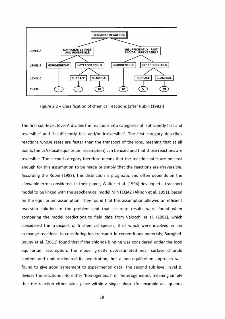
Figure 2.2 – Classification of chemical reactions (after Rubin (1983))
The first sub-level, level A divides the reactions into categories of ‘sufficiently fast and
reversible’ and ‘insufficiently fast and/or irreversible’. The first category describes
reactions whose rates are faster than the transport of the ions, meaning that at all
points the LEA (local equilibrium assumption) can be used and that those reactions are
reversible. The second category therefore means that the reaction rates are not fast
enough for this assumption to be made or simply that the reactions are irreversible.
According the Rubin (1983), this distinction is pragmatic and often depends on the
allowable error considered. In their paper, Walter et al. (1994) developed a transport
model to be linked with the geochemical model MINTEQA2 (Allison et al. 1991), based
on the equilibrium assumption. They found that this assumption allowed an efficient
two-step solution to the problem and that accurate results were found when
comparing the model predictions to field data from Valocchi et al. (1981), which
considered the transport of 5 chemical species, 3 of which were involved in ion
exchange reactions. In considering ion transport in cementitious materials, Baroghel-
Bouny et al. (2011) found that if the chloride binding was considered under the local
equilibrium assumption, the model greatly overestimated near surface chloride
content and underestimated its penetration; but a non-equilibrium approach was
found to give good agreement to experimental data. The second sub-level, level B,
divides the reactions into either ‘homogeneous’ or ‘heterogeneous’; meaning simply
that the reaction either takes place within a single phase (for example an aqueous
19
complexation) or between two or more phases (for example salt precipitation). The
final sub-level, level C, then divides the heterogeneous reactions into two types,
‘surface’ or ‘classical’, a surface reaction could involve adsorption onto the solid matrix
or ion exchange, whereas a classical reaction could include precipitation/dissolution,
complex formation or oxidation/reduction (Rubin 1983).
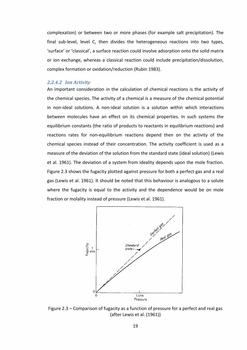
2.2.4.2 Ion Activity
An important consideration in the calculation of chemical reactions is the activity of
the chemical species. The activity of a chemical is a measure of the chemical potential
in non-ideal solutions. A non-ideal solution is a solution within which interactions
between molecules have an effect on its chemical properties. In such systems the
equilibrium constants (the ratio of products to reactants in equilibrium reactions) and
reactions rates for non-equilibrium reactions depend then on the activity of the
chemical species instead of their concentration. The activity coefficient is used as a
measure of the deviation of the solution from the standard state (ideal solution) (Lewis
et al. 1961). The deviation of a system from ideality depends upon the mole fraction.
Figure 2.3 shows the fugacity plotted against pressure for both a perfect gas and a real
gas (Lewis et al. 1961). It should be noted that this behaviour is analogous to a solute
where the fugacity is equal to the activity and the dependence would be on mole
fraction or molality instead of pressure (Lewis et al. 1961).
Figure 2.3 – Comparison of fugacity as a function of pressure for a perfect and real gas (after Lewis et al. (1961))
20
It can be seen then that the calculation of chemical activity can be of great importance
for chemical reaction calculations. To this end, theories of electrolyte solutions have
been proposed that seek to quantify the interactions between ions and hence the
effect these will have on the ideality of the solution. The most commonly used are
extended versions the Debye-Hückel theory such as the Davies equation (Allison et al.
1991; Samson and Marchand 2007b). Debye and Hückel (1923) assumed that the
solution consisted of a dielectric medium where the ions interact according to
Coulomb’s law. The theory assumes that the effect of the charge on an ion can be
calculated from a charge density given by Boltzmann’s law, and a charge distribution
described by Poisson’s equation, where there is spherical symmetry around an ion. In
solving these equations, a truncated Taylor series is used including only one term
which corresponds to 1-1 electrolytes such as NaCl (Lewis et al. 1961). The extended
Debye-Hückel law is given as (Koniorczyk 2012):
| |√
√ (2.10)
where A is a constant which depends on the solvent, I is the ionic strength and is
the average activity coefficient. As a result of these assumptions, and the fact that
short range interactions between ions are ignored, the Debye-Hückel theory is only
valid for dilute solutions (Koniorczyk 2012) and therefore at higher concentrations a
more comprehensive set of equations are needed. One such set of equations are the
Pitzer equations (Pitzer 1973). The Pitzer equations are formed through the virial
expansion of the Gibbs free energy of the solution, including a term representing the
extended Debye-Hückel theory and higher order terms which account for short range
interactions (Koniorczyk 2012). The simplified form of the Pitzer equation for
calculating the activity for an ion i is given as (Pitzer 1973):
∑
∑
∑ , (2.11)
where is a Debye-Hückel term, are molalities and , and are terms which
represent the interactions between ions. The second order terms in the expansion
represent all possible interactions between two ions, the third order terms
representing all possible interactions between three ions and so on (Koniorczyk 2012).
21
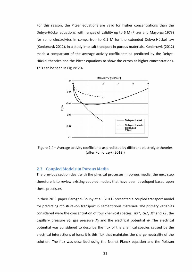
For this reason, the Pitzer equations are valid for higher concentrations than the
Debye-Hückel equations, with ranges of validity up to 6 M (Pitzer and Mayorga 1973)
for some electrolytes in comparison to 0.1 M for the extended Debye-Hückel law
(Koniorczyk 2012). In a study into salt transport in porous materials, Koniorczyk (2012)
made a comparison of the average activity coefficients as predicted by the Debye-
Hückel theories and the Pitzer equations to show the errors at higher concentrations.
This can be seen in Figure 2.4.
Figure 2.4 – Average activity coefficients as predicted by different electrolyte theories (after Koniorczyk (2012))
2.3 Coupled Models in Porous Media
The previous section dealt with the physical processes in porous media, the next step
therefore is to review existing coupled models that have been developed based upon
these processes.
In their 2011 paper Baroghel-Bouny et al. (2011) presented a coupled transport model
for predicting moisture-ion transport in cementitious materials. The primary variables
considered were the concentration of four chemical species, Na+, OH-, K+ and Cl-, the
capillary pressure PC, gas pressure Pg and the electrical potential ψ. The electrical
potential was considered to describe the flux of the chemical species caused by the
electrical interactions of ions; it is this flux that maintains the charge neutrality of the
solution. The flux was described using the Nernst Planck equation and the Poisson
22
equation was used to describe the electrical potential. The ion activity was included in
the model and its effect on the water/water vapour equilibrium was taken into
account. The ion activities were calculated based on a combination of long range
effects (Debye-Hückel and Davies equations) and short range (Pitzer equations). The
concentration of the chemical species was assumed not to have any effect on the
moisture retention curve based on the results of experimental adsorption data; their
effect was, however, taken into account on both the viscosity of the fluid -via a Jones-
Doyle type equation- and the fluid density. The permeability of the moisture phase
was calculated using Mualem’s model (Mualem 1976), as opposed to the analytical
form derived by van Genuchten (van Genuchten 1980), as the former is valid for both
adsorption and desorption, when the latter is valid for adsorption only. Following
experimental results on desorption it was found that for moisture contents of Sw<0.4
the relative permeability greatly dropped and so liquid transport was assumed not to
take place below this value. The reactions considered were of the chloride binding
onto the C-S-H and the formation of Freidel’s salt. These reactions were calculated
with assumptions of both equilibrium and non-equilibrium conditions and compared to
experimental data for the total chloride content. It was found that under the
equilibrium assumption the model greatly over predicted the chloride content at the
surface and under predicted its penetration into the mortar samples, the best results
were found when the chloride binding was considered kinetically and the Freidel’s salt
formation as instantaneous.
In investigating the transport and precipitation of salt in porous building materials,
Koniorczyk (2010; 2012) developed a finite element model based on the volume
averaged governing balance equations. These included the mass balance of moisture,
dry air and solute, the enthalpy balance equation for temperature and the linear
momentum conservation equation for deformation. The chosen primary variables
were capillary pressure PC, gas pressure Pg, chemical concentration c, temperature T
and displacement u. The mathematical model was an extension of previous work
(Gawin et al. 1996; Lewis and Schrefler 1998). The salt concentration was assumed
here to affect the dynamic viscosity and density of the fluid as well as the moisture
retention curve, the effect of which was studied in an earlier paper (Koniorczyk and
23
Wojciechowski 2009). In the latter paper (Koniorczyk 2012), the salt crystallisation was
taken into account with an assumption of non-equilibrium conditions and the rate of
precipitation is given by the Freundlich type isotherm based on the supersaturation of
the solution. The supersaturation was calculated as function of ion activity and the
equilibrium constant of the reaction K. Due to its accuracy at the concentration levels
found during the drying of porous media investigated; the Pitzer model was chosen to
calculate the activities of the ions. Three further phenomena were considered, the first
of which is the heat of reaction -as salt precipitation is an exothermic reaction- which
was included in the enthalpy balance equation. The second is the reduction in pore
space due to the presence of the salt crystals, this was taken into account through a
simplified method developed by the author in an earlier paper (Koniorczyk and Gawin
2008). The third is the crystallisation pressure on the solid skeleton. This arises as a
result of the fact that the solid skeleton confines the salt crystal between the pore
walls. The crystallisation pressure was calculated as the difference between the
pressure on the loaded crystal face and the hydrostatic pressure. The value of this
crystallisation pressure was derived from the chemical potential of the unloaded and
loaded sides of the crystal and of the solute, leading to the pressure as a function of
the activity, molar volume of the crystal and the equilibrium constant.
In 2014, Song et al. (2014) presented a finite difference model to study the diffusion
and reaction of six chemical species namely OH-, Na+, K+, Cl-, Ca2+ and SO42- , whilst
also taking into account the interaction between ions. The interaction between the
ions was taken into account through the diffusive flux of ions due to the local electrical
field, described by the Nernst Planck equation, and the local electric field is described
by the Poisson equation, as in (Baroghel-Bouny et al. 2011). The difference here is that,
instead of solving for the electrical potential ψ as a primary variable, Song et al. (2014)
asserted that if the initial solution is charge neutral then the charge neutrality
condition is the condition of zero current. This allowed the rearrangement of the sum
of the diffusive flux of all chemicals for the gradient of electrical potential, which was
then substituted into the Nernst Planck equation. The effect of electrostatic double
layers was also taken into account by applying a factor to the molecular diffusion
coefficients. There were a number of chemical reactions that were considered, all
24
based on an assumption of non-equilibrium conditions. The rates of reaction were
empirical but all based on mass action law or something like mass action law, where
the Freundlich type isotherm was used for their calculation. There were a number of
chemical reactions that were taken into consideration including the dissolution of the
cement phases. The dissolution of portlandite was included, which occurs due to the
concentration difference in calcium between the pore and source solutions as was the
dissolution of calcium and hydroxide from the C-S-H phases. The chemical chloride
bindings onto the AFm phases were considered, including formation of Freidel’s salt
and Kuzel’s salt, both of which are said to be just special formulas of the AFm phases,
meaning that the chemical chloride binding can be seen as just the creation or
transformation of this phase (Song et al. 2014). The physical absorption of the chloride
ions onto the C-S-H phases was also taken into account; however, their chemical
binding onto the same phase was not considered. Finally, the alkali bindings onto both
the C-S-H and AFm phases have been included, the former of which is said to have a
significant effect on the chloride diffusion.
2.4 Reduced Models in Porous Media
The computational cost of solving the coupled models used for this kind of transport
problem can become quite large for particular chemical systems. According to Cleall et
al. (2006) this is driven by three main areas, the domain size, time scale and complexity
of the analysis; where the complexity of the analysis is dependent on the number of
variables and degree of coupling between them, the non-linearity of the system and
the number of processes considered. A number of authors deal with this problem by
using an operator splitting scheme, changing the numerical treatment of the problem
from a GIA (Global Implicit Approach) to an SIA or SNIA (Sequential Iterative Approach
or Sequential Non-iterative Approach) (Yeh and Tripathi 1991; Walter et al. 1994; Cleall
et al. 2007; Beisman et al. 2015; Yapparova et al. 2017).
GIAs are one step methods that solve the governing equations of transport (PDE’s,
which are coupled through reaction terms) and chemical reactions (ODE’s, which are
also coupled through reaction terms or AE’s) simultaneously. Two common methods of
doing this are the DAE (mixed differential and algebraic equation) method, where the
mixed differential and algebraic equations are solved simultaneously for the primary
25
dependant variables, and the DSA (direct substitution approach), in which -where
possible- the nonlinear chemical reactions are substituted directly into the transport
equations, reducing the system to a set of nonlinear PDE’s (Yeh and Tripathi 1989). In
the latter method the AE’s can be solved for certain variables, which can then be
eliminated from the differential equations (Kräutle and Knabner 2005).
SIA/SNIA methods are two step methods which solve the governing equations of
transport first and then calculate the chemical reactions, where the SIA will then
iterate between the two over a time step. One of the attractions of SIA/SNIA methods
is that they have been found to reduce the computational cost, placing less demand on
CPU memory and CPU time (Yeh and Tripathi 1989). The problem with operator
splitting approaches is that the SNIA can introduce a splitting error and the SIA can
require a prohibitively small time step and a large number of iterations in order to
converge (Kräutle and Knabner 2007; Hoffmann et al. 2012). The accuracy of operator
splitting was discussed in detail by Valocchi and Malmstead (1992) who found that for
continuous mass influx boundary conditions there is an inherent mass balance error
that was proportional to the time step size and the decay constant (for a first order
decay problem). It was found however that with a reversal of order of the steps at
each time step this error could be reduced to less than 10 % of its value.
Due to the potential problems with operator splitting methods, a number of authors
have instead turned their attention to approaches that can reduce the computational
cost of the global methods, usually through reformulating the system to reduce the
number of coupled PDE’s and eliminating a number of local equations (Friedly and
Rubin 1992; Molins et al. 2004; Hoffmann et al. 2012; Huo et al. 2014). The
reformulation of the system is usually achieved using the stoichiometric matrix and
variable transforms. The problem with this approach is that the amount of reduction
that can be achieved often depends on the problem chemistry and many impose the
condition of equal diffusion coefficients. A review of some operator splitting models
and reduced order global models will be presented in the following subsections.
26
2.4.1 Operator Splitting
In 1991 Yeh and Tripathi (1991) presented a numerical model based on the governing
mass balance equations of aqueous and sorbed concentration and cation exchange
capacity. The chemical reactions were considered with an assumption of equilibrium
conditions, based on the laws of mass action, taking into account the deviation from
ideality of the solution through the activity coefficients. The activity coefficients were
calculated using the Davies equation which is valid up to concentrations of 0.3 M. The
model was developed such that a number of different types of chemical reactions
could be considered including complexation, adsorption, ion exchange,
precipitation/dissolution, redox, and acid-base reactions. The SIA method was chosen
for the numerical treatment of the problem, where the transport was separated from
the chemical reactions. The algorithm employed calculated any sorption reactions at
the beginning of the time step, and then iterated between the transport, and
remaining reactions until a convergence tolerance was met. Yeh and Tripathi (1991)
assert that the choice of primary dependant variables (PDV’s) is of great importance as
it can determine how practically it can be used for realistic problems and how many of
the different types of chemical reactions it can model. The total analytical
concentrations were chosen here as the PDV’s as this allows for
precipitation/dissolution reactions.
Walter et al. (1994) presented a numerical model for predicting the reactive chemical
transport in groundwater systems, called MINTRAN in 1994. This model was a
combination of a transport model PLUME2D (Frind et al. 1990) and a geochemical
model, namely MINTEQA2 (Allison et al. 1991). The numerical treatment of the model
was considered in two ways, both a SIA and a SNIA. The SIA method solved the
transport of the components first taking the reaction as constant, then the reactions,
taking the physical terms as constant. The spatial terms in this method were centrally
weighted for greater accuracy, and for consistency so was the reaction term. For the
SNIA method the transport is again calculated first, with the central weighting for the
spatial terms; however, this time the reaction term was not included. Following this,
the chemical reactions were calculated at the end of the time step. The accuracy of the
two approaches was compared and it was found that the SNIA took 1 hour and the SIA
27
3.5 hours CPU time on an IBM 6000/560, with only 2 % difference in the results
profiles. The governing equations were considered for the component concentrations
in order to reduce the size of the system, as the components are the minimum number
of species that are needed to solve the system. The chemical reactions were
considered with an assumption of non-equilibrium conditions and were calculated
based on the mass action laws, as a function of the activity coefficients.
A coupled Thermo/Hydro/Chemical/Mechanical model was presented by Cleall et al.
(2007) for unsaturated soils. The primary variables considered were the pore water
pressure Pw, pore air pressure Pa, temperature T, dissolved chemical concentration c,
and the displacement u. The mathematical development of the model was based on
previous work by Thomas and He (1995; 1997).The liquid moisture transfer considered
the advection described using Darcy’s law as well as the osmotic flow, which is the
diffusion of the liquid driven by the chemical concentration gradients, where the fluid
will diffuse to areas of higher concentration. The relative permeability of the medium
was calculated using Kozeny’s approach. Concerning the heat transfer, the conduction
and convection were taken into account whilst the radiation and the transfer of heat
due to chemical concentration gradients were neglected following the conclusions of
previous authors as to their significance (Mitchell 1993). The chemical mass balance
considered the advection, dispersion and reaction of the solutes, where the
temperature dependence of the diffusion coefficients as well as the Soret effect, or
chemical diffusion due to temperature gradients was included. The chemical reactions
were assumed to be sufficiently fast such that the local equilibrium assumption could
be made and were calculated through coupling the model to the geochemical model
MINTEQA2. Both the SIA and SNIA methods were used for the numerical treatment of
the problem. The model was then tested against an example problem involving
dolomisation, where a 1D domain saturated with an aqueous solution was flushed by
water of a different chemical composition. The predicted profiles were then compared
to the results of Engesgaard and Kipp (1992). It was found that the models agreed very
closely, with the exception of the sharp mineral fronts. It was thought that this
difference was attributable to the fact that Engesgaard and Kipp (1992) included an
algorithm in their model to avoid numerical instabilities.
28
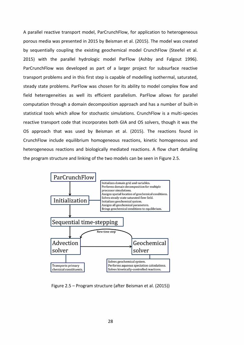
A parallel reactive transport model, ParCrunchFlow, for application to heterogeneous
porous media was presented in 2015 by Beisman et al. (2015). The model was created
by sequentially coupling the existing geochemical model CrunchFlow (Steefel et al.
2015) with the parallel hydrologic model ParFlow (Ashby and Falgout 1996).
ParCrunchFlow was developed as part of a larger project for subsurface reactive
transport problems and in this first step is capable of modelling isothermal, saturated,
steady state problems. ParFlow was chosen for its ability to model complex flow and
field heterogeneities as well its efficient parallelism. ParFlow allows for parallel
computation through a domain decomposition approach and has a number of built-in
statistical tools which allow for stochastic simulations. CrunchFlow is a multi-species
reactive transport code that incorporates both GIA and OS solvers, though it was the
OS approach that was used by Beisman et al. (2015). The reactions found in
CrunchFlow include equilibrium homogeneous reactions, kinetic homogeneous and
heterogeneous reactions and biologically mediated reactions. A flow chart detailing
the program structure and linking of the two models can be seen in Figure 2.5.
Figure 2.5 – Program structure (after Beisman et al. (2015))
29
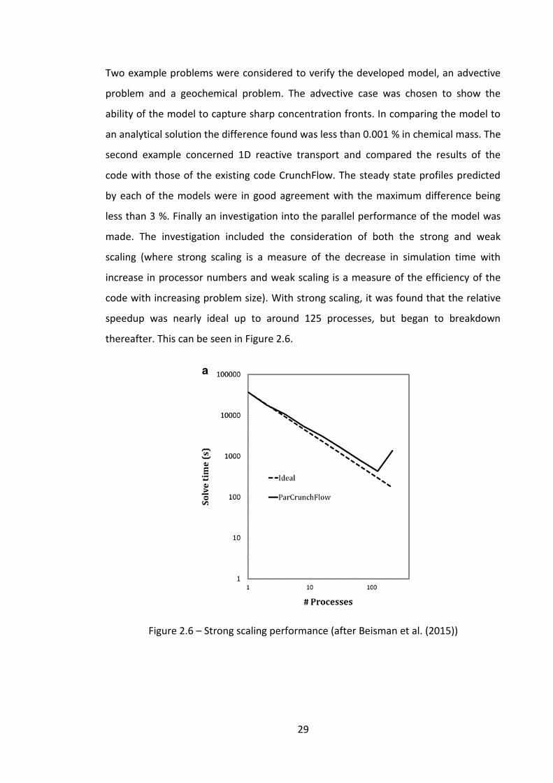
Two example problems were considered to verify the developed model, an advective
problem and a geochemical problem. The advective case was chosen to show the
ability of the model to capture sharp concentration fronts. In comparing the model to
an analytical solution the difference found was less than 0.001 % in chemical mass. The
second example concerned 1D reactive transport and compared the results of the
code with those of the existing code CrunchFlow. The steady state profiles predicted
by each of the models were in good agreement with the maximum difference being
less than 3 %. Finally an investigation into the parallel performance of the model was
made. The investigation included the consideration of both the strong and weak
scaling (where strong scaling is a measure of the decrease in simulation time with
increase in processor numbers and weak scaling is a measure of the efficiency of the
code with increasing problem size). With strong scaling, it was found that the relative
speedup was nearly ideal up to around 125 processes, but began to breakdown
thereafter. This can be seen in Figure 2.6.
Figure 2.6 – Strong scaling performance (after Beisman et al. (2015))
30
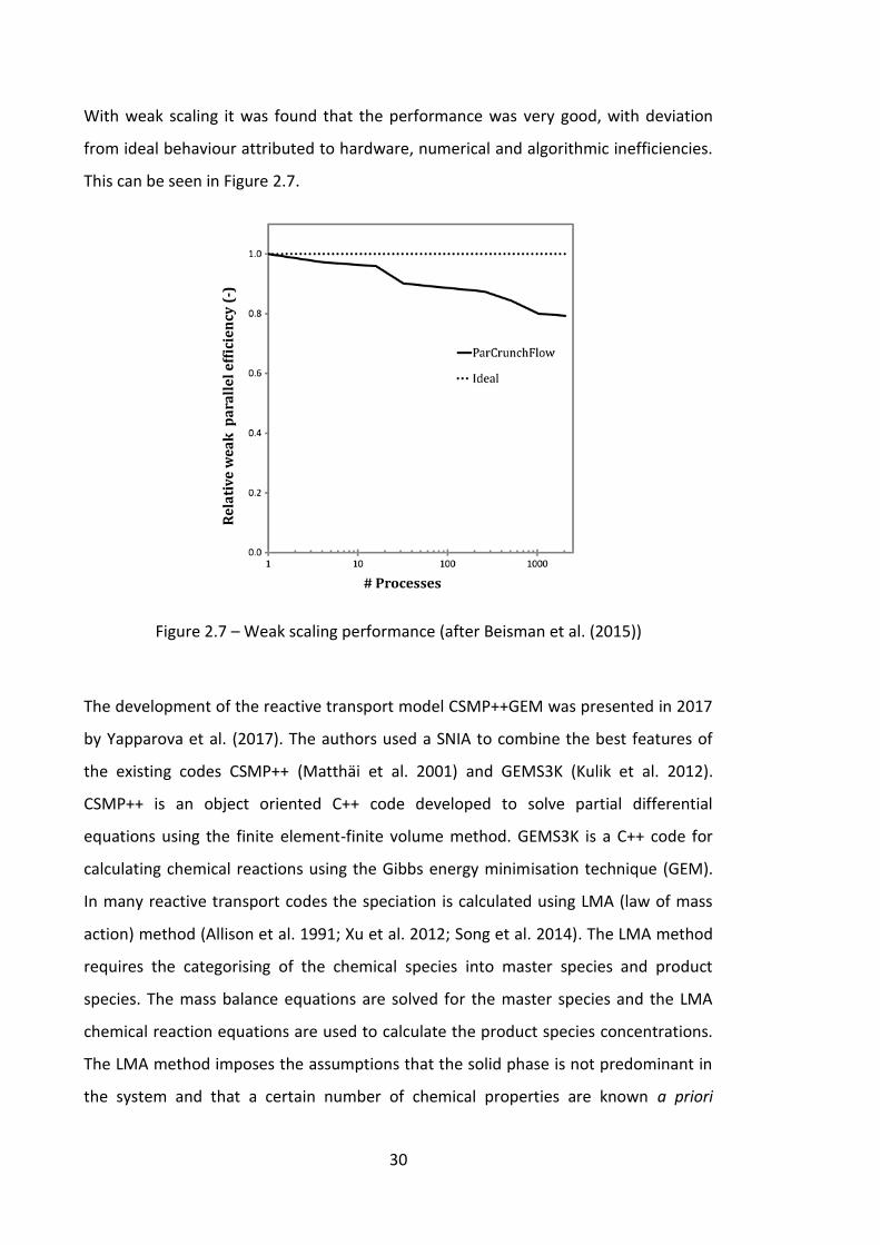
With weak scaling it was found that the performance was very good, with deviation
from ideal behaviour attributed to hardware, numerical and algorithmic inefficiencies.
This can be seen in Figure 2.7.
Figure 2.7 – Weak scaling performance (after Beisman et al. (2015))
The development of the reactive transport model CSMP++GEM was presented in 2017
by Yapparova et al. (2017). The authors used a SNIA to combine the best features of
the existing codes CSMP++ (Matthäi et al. 2001) and GEMS3K (Kulik et al. 2012).
CSMP++ is an object oriented C++ code developed to solve partial differential
equations using the finite element-finite volume method. GEMS3K is a C++ code for
calculating chemical reactions using the Gibbs energy minimisation technique (GEM).
In many reactive transport codes the speciation is calculated using LMA (law of mass
action) method (Allison et al. 1991; Xu et al. 2012; Song et al. 2014). The LMA method
requires the categorising of the chemical species into master species and product
species. The mass balance equations are solved for the master species and the LMA
chemical reaction equations are used to calculate the product species concentrations.
The LMA method imposes the assumptions that the solid phase is not predominant in
the system and that a certain number of chemical properties are known a priori
31
including the redox state of stable phases. In contrast the GEM calculates the
speciation based on the elemental bulk composition of the system, through the
minimisation of the systems total Gibbs energy. The advantage of the GEM over the
LMA is that it does not hold the aforementioned assumptions. The model was then
applied to two 1D benchmarking problems involving dolomisation. The latter case
involved the dolomisation by sea water and considered mineral kinetics. The authors
compared the results of their model to those of TOUGHREACT (Xu et al. 2012) and
found that the results were similar. The minor differences were put down to the
following (i) TOUGHREACT uses a finite difference method whereas CSMP++GEM uses
a finite element-finite volume method, (ii) chemical reactions were calculated
differently (LMA vs GEM), (iii) different thermodynamic databases were used with
different aqueous activity and mineral kinetic rate models and (iv) there are
differences in the equations of state for the aqueous fluid.
2.4.2 Reduced Order GIA
Friedly and Rubin (1992) in 1992 presented an approach to simulate reactive chemical
transport that resulted in a compact form of the governing equations. The approach is
based on the consideration of the concentration and reactions as vector spaces and
uses the stoichiometry of the problem to reduce the system of equations. This
approach was based on the work for batch systems by Thompson (1982a; 1982b) and
its extension to flow by Friedly (1991). The model is applicable to both equilibrium and
non-equilibrium reactions, but requires that the advection-dispersion operator acts on
all solutes in the same way. The first step to the development was to define vectors of
the concentrations of mobile species, concentrations of immobile species, reaction
rates, and stoichiometric coefficients of both mobile and immobile species. Then
defining a vector of all concentrations and a matrix of all stoichiometric coefficients S,
the mass balance equations for mobile and immobile species can be written in vector
form.
[
] (2.12)
where L is the transport operator and I is the identity matrix. This is done in order to
take advantage of linear algebra of vector spaces. The next step was to break down the
32
vector of concentration X, which represents the concentration space into a set of basis
vectors, given for the example of the choice of Cartesian coordinates as the basis
vectors as:
[ ] [
] (2.13)
In actuality, any complete set of linearly independent vectors may be chosen, and
following the approach for batch reaction systems the columns of the stoichiometric
matrix S are chosen by the author, representing the reaction space. These alone are
not enough and are supplemented by the orthogonal matrix , giving:
(2.14)
where ξ and η are factors analogous to and and represent the extent of the
reactions and the reaction invariants respectively. This can be applied similarly to the
mobile species only to give ξm and ηm, where the m subscript denotes mobile
contributions. This leads to the equivalent form of X as:
[ ] [
] (2.15)
where the overbar indicates immobile species. This can then be substituted into the
original mass balance equation, leading to the following set of equations to be solved:
( , , , ) (2.16)
( ) (2.17)
(2.18)
where the superior dot denotes the time derivative, A is a matrix depending on the
stoichiometry and ξ, ξm and ηm are the PDV’s of the system, η is not considered as a
variable as it can often be determined from the initial conditions alone and, for a
spatially uniform initial state remain unchanged, and so is often neglected. This
reformulation of the equations has eliminated the reaction rates and immobile species
concentrations from the PDE’s. Leading to a system of J chemical reaction equations
33
(one for each reaction) for ξ, Jmind (number of linearly independent reactions in their
mobile phase stoichiometry) linear PDE’s for ξm -coupled indirectly through the
reaction extent ξ- and I-Jmind (where I is the number of mobile species) linear
uncoupled PDE’s for ηm. The chemical concentrations can then be calculated from the
PDV’s.
A decoupling method for application to both SIA and DSA methods was presented by
Molins et al. (2004) in 2004. Molins et al. (2004) point to the fact that difficulties are
caused by the coupling between the transport equations, causing the DSA to be
inefficient for large systems (Yeh and Tripathi 1989) and convergence issues for the SIA
for some systems such that the DSA is preferred (Saaltink et al. 2001). The beginning of
their approach is to set the problem into vector space following the work of Friedly
and Rubin (1992) discussed previously, before defining components to eliminate any
coupling terms. The approach is split into four distinct paradigms, where a different
construction of the component matrix is proposed for each, depending on the
chemical treatment of the system. The first paradigm is the tank paradigm and
considers only mobile species with equilibrium reactions that take place within the
aqueous phase. The second is the canal paradigm, which is the tank paradigm with
some kinetic reactions. The third is a river paradigm in which heterogeneous reactions
are now included, but are kinetically controlled. The final paradigm is of an aquifer in
which heterogeneous reactions can also be considered as equilibrium reactions. For
the tank system the governing equations are simply multiplied by the equilibrium
component matrix (made up of the identity matrix and equilibrium stoichiometry),
eliminating the reaction rates and thus uncoupling the system. Leading to a system of
Je (where Je is the number of equilibrium equations) AE’s describing the reactions and
of I-Je linear uncoupled PDE’s for conservative components given as:
(2.19)
where are the chemical components for this paradigm. The transport of the
components can therefore be solved separately and the nonlinear system of AE’s for
the chemical reactions solved for each node separately. For the canal system, the
governing equations can then be multiplied by the kinetic component matrix (made up
34
of the identity matrix and kinetic stoichiometry) which leads to a system of Je (where Je
is the number of equilibrium equations) AE’s describing the equilibrium reactions, Jk
(where Jk is the number of kinetic reactions) ODE’s describing the kinetic reactions, I-
Je-Jk linear uncoupled PDE’s for conservative components and Jk PDE’s. The system is
given as:
(2.20)
(2.21)
where and
are the chemical components for this paradigm and are the
kinetic reaction rates. For the river system a factor matrix is developed to eliminate the
immobile kinetic species from the components. This factor matrix is derived by
splitting of the component matrix into two arbitrary groups of conservative
components and mobile and immobile groups of the kinetic components. The factor
matrix can then be found as the inverse of this component matrix. This factor matrix
and the component matrix from the canal paradigm can then be multiplied by the
governing equations to decouple them, leading to a reduction to a system of Je (where
Je is the number of equilibrium equations) AE’s describing the equilibrium reactions,
Jk+Jki ODE’s describing the kinetic reactions, I-Je-Jk-Jki (where Jki is the number of
kinetic reactions involving immobile species) linear uncoupled PDE’s for conservative
components and Jk PDE’s. The system is given as:
(2.22)
(
) (2.23)
where and
are the chemical components for this paradigm, M is a matrix
of coefficients of 1 for mobile and 0 for immobile species, are the kinetic reaction
rates for aqueous species, are the reaction rates for immobile species and
is the
kinetic component matrix for immobile species. The final paradigm is the aquifer
system, the treatment of which is similar to that of the river paradigm in that a matrix
is derived based on the restructuring of the components matrix and multiplied by the
35
system to eliminate some species. The species being eliminated in this paradigm are
the fixed activity species such as minerals.
(2.24)
(
) (2.25)
where
and
are the chemical components for this paradigm. It should
be noted that this only applies to fixed activity species and so any adsorbed species
would not be eliminated as their activity is not fixed. An investigation into the
efficiency of the approach when implemented into a DSA and an SIA was made and the
authors found that both benefited from the decoupling, but especially the DSA.
In 2012, Hoffman et al. (2012) presented a general reduction scheme for reactive
transport based on linear transformation of the equations and variables. The model
was an extension on the previous work of two of the authors (Kräutle and Knabner
2005; Kräutle and Knabner 2007; Kräutle 2008). The model assumes that the diffusion
coefficient is the same for all species, and is justified by the fact that the molecular
diffusion is usually small in comparison to the mechanical dispersion. The
stoichiometric matrix is filled in in a particular order and is split into four parts, a)
mobile species with equilibrium reactions, b) mobile species with kinetic reactions, c)
immobile species with equilibrium reactions and d) immobile species with kinetic
reactions. These sections are then also filled in a particular order; section a) starts with
the reactions with only mobile species, followed by sorption reactions and then
mineral reactions. Section c) is ordered similarly but without the mobile species
reactions. The reformulation begins by defining two matrices, S1 and S2 that represent
the maximal system of linearly independent columns of the mobile and immobile
sections of the stoichiometric matrix respectively. The decoupling of some PDE’s
results from the multiplication of the governing equations by matrices and
,
followed by a transformation of variables. The matrices are not defined but instead a
list of conditions for their choice is presented including the linear dependence of all of
the columns of each and the fact that all of the columns of are orthogonal to all
columns of S1. Following their multiplication by the system of PDE’s transformed
36
variables are chosen ξm and ηm, where ηm are reaction invariants. This leads to the
elimination of the mobile species equilibrium reaction rates, reducing the system. The
next step was to apply this to the system of ODE’s for the immobile species, which lead
to another set of transformed variables and η, where η are reaction invariant. The
equations for reaction invariants are decoupled and linear and the mobile equilibrium
reaction rates have been eliminated, however the sorption and mineral equilibrium
reaction rates remain. The elimination of these reaction rates is achieved by the
introduction of additional variables , these new variables allow equations to be solved
for the aforementioned reaction rates, which can then be substituted into the PDE’s.
The final reduction of the system is made through the consideration of the local
equations. Using a resolution function a number of these local equations can also be
eliminated. This leads to a system of equations of Im-Jm-Jsorp-Jmin-Jkin (where Im is the
number of mobile species, Jm is the number of chemical reactions involving only
mobile species, Jsorp is the number of sorption reactions, Jmin is the number of mineral
reactions and Jkin is the number of kinetic reactions) PDE’s for , I-Jsorp-Jmin-Jkin
(where I is the number of immobile species) PDE’s for and Jsorp+Jmin+Jkin PDE’s and
Jsorp+Jmin+Jkin AE’s for given as:
(2.26)
(2.27)
( ) (2.28)
( ) (2.29)
The efficiency of the resultant scheme was tested on the MoMaS benchmark
(Carrayrou et al. 2010) 2D advective easy test case, and compared against the results
from the code HYTEC (SIA) (Lagneau and van der Lee 2010) and MIN3P (DSA) (Mayer
and MacQuarrie 2010). The proposed reduction scheme was found to be five times
faster than those of both HYTEC and MIN3P when comparing the normalised CPU time.
In 2014 Huo et al. (2014) presented a decoupling approach for application to reactive
transport in heterogeneous porous media. The idea of the approach was to split the
domain into a number of sub-domains based on the spatial variance of the physical
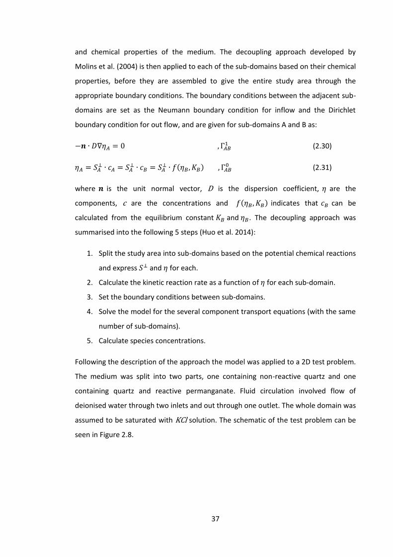
37
and chemical properties of the medium. The decoupling approach developed by
Molins et al. (2004) is then applied to each of the sub-domains based on their chemical
properties, before they are assembled to give the entire study area through the
appropriate boundary conditions. The boundary conditions between the adjacent sub-
domains are set as the Neumann boundary condition for inflow and the Dirichlet
boundary condition for out flow, and are given for sub-domains A and B as:
, (2.30)
( , ) ,
(2.31)
where is the unit normal vector, D is the dispersion coefficient, are the
components, c are the concentrations and ( , ) indicates that can be
calculated from the equilibrium constant and . The decoupling approach was
summarised into the following 5 steps (Huo et al. 2014):
1. Split the study area into sub-domains based on the potential chemical reactions
and express and for each.
2. Calculate the kinetic reaction rate as a function of for each sub-domain.
3. Set the boundary conditions between sub-domains.
4. Solve the model for the several component transport equations (with the same
number of sub-domains).
5. Calculate species concentrations.
Following the description of the approach the model was applied to a 2D test problem.
The medium was split into two parts, one containing non-reactive quartz and one
containing quartz and reactive permanganate. Fluid circulation involved flow of
deionised water through two inlets and out through one outlet. The whole domain was
assumed to be saturated with KCl solution. The schematic of the test problem can be
seen in Figure 2.8.
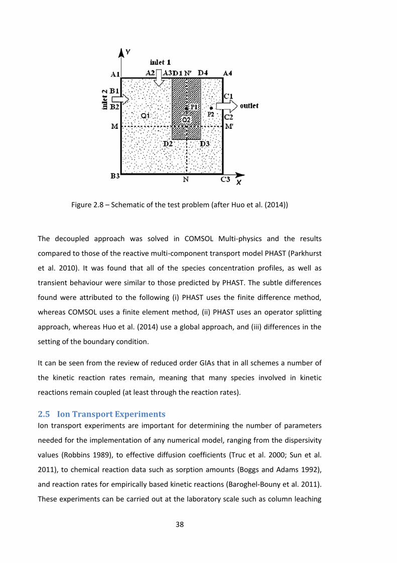
38
Figure 2.8 – Schematic of the test problem (after Huo et al. (2014))
The decoupled approach was solved in COMSOL Multi-physics and the results
compared to those of the reactive multi-component transport model PHAST (Parkhurst
et al. 2010). It was found that all of the species concentration profiles, as well as
transient behaviour were similar to those predicted by PHAST. The subtle differences
found were attributed to the following (i) PHAST uses the finite difference method,
whereas COMSOL uses a finite element method, (ii) PHAST uses an operator splitting
approach, whereas Huo et al. (2014) use a global approach, and (iii) differences in the
setting of the boundary condition.
It can be seen from the review of reduced order GIAs that in all schemes a number of
the kinetic reaction rates remain, meaning that many species involved in kinetic
reactions remain coupled (at least through the reaction rates).
2.5 Ion Transport Experiments
Ion transport experiments are important for determining the number of parameters
needed for the implementation of any numerical model, ranging from the dispersivity
values (Robbins 1989), to effective diffusion coefficients (Truc et al. 2000; Sun et al.
2011), to chemical reaction data such as sorption amounts (Boggs and Adams 1992),
and reaction rates for empirically based kinetic reactions (Baroghel-Bouny et al. 2011).
These experiments can be carried out at the laboratory scale such as column leaching
39
experiments (Wierenga and Van Genuchten 1989; Krueger et al. 1998; Hartley et al.
2004; Liu et al. 2017) used for geochemical data, or at the field scale, for example, to
determine the scale effect of dispersion (Domenico and Robbins 1984). It is the
laboratory scale experiments that are of interest here as this is the scale of the
experimental procedure developed in this thesis.
For the determination of these parameters in soils, column leaching experiments have
been used by a number of authors (Robbins 1989; Wierenga and Van Genuchten 1989;
Krueger et al. 1998; Hartley et al. 2004; Liu et al. 2017). In 1989 Wierenga and van
Genutchen (1989) published a study into solute transport into small and large soil
columns to determine the dispersion coefficients, dispersivity coefficients and
retardation factors for the transport of a Ca(NO3)2 solution through columns, filled
with a Berino loamy fine sand, at four different moisture contents. The retardation
factor accounts for interactions between the solute and the soil matrix, for example
the physical adsorption. The experimental procedure was to apply a tracer to the
columns at a constant rate and measure the concentration in the effluent collected
from the outflow, the parameters can then be determined through an optimisation
program. For the small column experiments, Plexiglas columns of 5.1 cm diameter and
30 cm length were used. The ends of the columns were sealed with porous stainless
steel plates, held in place by Plexiglas end plates. The soil was air dried and passed
through a 1 mm sieve before placement. A vacuum was applied to the base of the
column, which was used to adjust the pressure to give equal pressure heads at the top
and the bottom of the column. The large column experiments were carried out in a 6
m long column made from galvanised highway culverts, with the setup being similar to
that of the small columns, with the main difference here being that suction candles
were placed at 6 depths through the column, allowing measurement at different
depths. The setup can be seen in Figure 2.9.
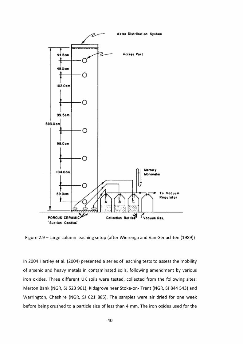
40
Figure 2.9 – Large column leaching setup (after Wierenga and Van Genuchten (1989))
In 2004 Hartley et al. (2004) presented a series of leaching tests to assess the mobility
of arsenic and heavy metals in contaminated soils, following amendment by various
iron oxides. Three different UK soils were tested, collected from the following sites:
Merton Bank (NGR, SJ 523 961), Kidsgrove near Stoke-on- Trent (NGR, SJ 844 543) and
Warrington, Cheshire (NGR, SJ 621 885). The samples were air dried for one week
before being crushed to a particle size of less than 4 mm. The iron oxides used for the
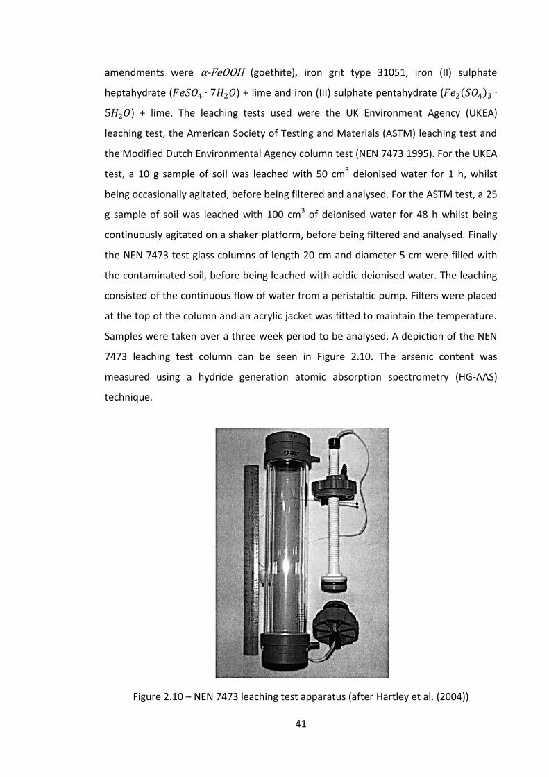
41
amendments were α-FeOOH (goethite), iron grit type 31051, iron (II) sulphate
heptahydrate ( ) + lime and iron (III) sulphate pentahydrate ( ( )
) + lime. The leaching tests used were the UK Environment Agency (UKEA)
leaching test, the American Society of Testing and Materials (ASTM) leaching test and
the Modified Dutch Environmental Agency column test (NEN 7473 1995). For the UKEA
test, a 10 g sample of soil was leached with 50 cm3 deionised water for 1 h, whilst
being occasionally agitated, before being filtered and analysed. For the ASTM test, a 25
g sample of soil was leached with 100 cm3 of deionised water for 48 h whilst being
continuously agitated on a shaker platform, before being filtered and analysed. Finally
the NEN 7473 test glass columns of length 20 cm and diameter 5 cm were filled with
the contaminated soil, before being leached with acidic deionised water. The leaching
consisted of the continuous flow of water from a peristaltic pump. Filters were placed
at the top of the column and an acrylic jacket was fitted to maintain the temperature.
Samples were taken over a three week period to be analysed. A depiction of the NEN
7473 leaching test column can be seen in Figure 2.10. The arsenic content was
measured using a hydride generation atomic absorption spectrometry (HG-AAS)
technique.
Figure 2.10 – NEN 7473 leaching test apparatus (after Hartley et al. (2004))
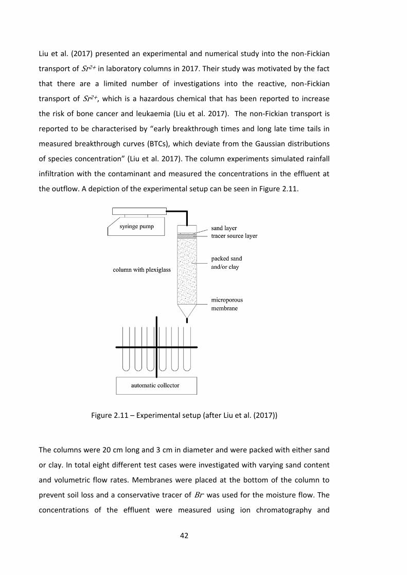
42
Liu et al. (2017) presented an experimental and numerical study into the non-Fickian
transport of Sr2+ in laboratory columns in 2017. Their study was motivated by the fact
that there are a limited number of investigations into the reactive, non-Fickian
transport of Sr2+, which is a hazardous chemical that has been reported to increase
the risk of bone cancer and leukaemia (Liu et al. 2017). The non-Fickian transport is
reported to be characterised by “early breakthrough times and long late time tails in
measured breakthrough curves (BTCs), which deviate from the Gaussian distributions
of species concentration” (Liu et al. 2017). The column experiments simulated rainfall
infiltration with the contaminant and measured the concentrations in the effluent at
the outflow. A depiction of the experimental setup can be seen in Figure 2.11.
Figure 2.11 – Experimental setup (after Liu et al. (2017))
The columns were 20 cm long and 3 cm in diameter and were packed with either sand
or clay. In total eight different test cases were investigated with varying sand content
and volumetric flow rates. Membranes were placed at the bottom of the column to
prevent soil loss and a conservative tracer of Br- was used for the moisture flow. The
concentrations of the effluent were measured using ion chromatography and
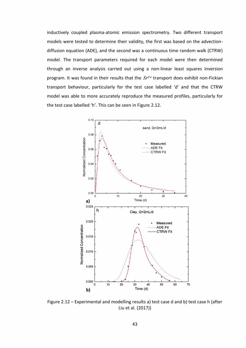
43
inductively coupled plasma-atomic emission spectrometry. Two different transport
models were tested to determine their validity, the first was based on the advection-
diffusion equation (ADE), and the second was a continuous time random walk (CTRW)
model. The transport parameters required for each model were then determined
through an inverse analysis carried out using a non-linear least squares inversion
program. It was found in their results that the Sr2+ transport does exhibit non-Fickian
transport behaviour, particularly for the test case labelled ‘d’ and that the CTRW
model was able to more accurately reproduce the measured profiles, particularly for
the test case labelled ‘h’. This can be seen in Figure 2.12.
Figure 2.12 – Experimental and modelling results a) test case d and b) test case h (after Liu et al. (2017))
a)
b)
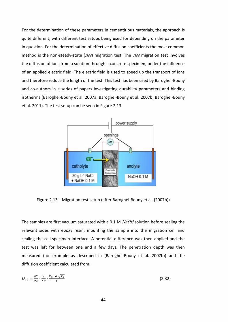
44
For the determination of these parameters in cementitious materials, the approach is
quite different, with different test setups being used for depending on the parameter
in question. For the determination of effective diffusion coefficients the most common
method is the non-steady-state (nss) migration test. The nss migration test involves
the diffusion of ions from a solution through a concrete specimen, under the influence
of an applied electric field. The electric field is used to speed up the transport of ions
and therefore reduce the length of the test. This test has been used by Baroghel-Bouny
and co-authors in a series of papers investigating durability parameters and binding
isotherms (Baroghel-Bouny et al. 2007a; Baroghel-Bouny et al. 2007b; Baroghel-Bouny
et al. 2011). The test setup can be seen in Figure 2.13.
Figure 2.13 – Migration test setup (after Baroghel-Bouny et al. (2007b))
The samples are first vacuum saturated with a 0.1 M NaOH solution before sealing the
relevant sides with epoxy resin, mounting the sample into the migration cell and
sealing the cell-specimen interface. A potential difference was then applied and the
test was left for between one and a few days. The penetration depth was then
measured (for example as described in (Baroghel-Bouny et al. 2007b)) and the
diffusion coefficient calculated from:
√
(2.32)

45
where Z is the valence of the ion, e is the thickness of the sample, t is the test
duration, is the applied potential, is a function of the test conditions, is the
penetration depth and is the effective chlorine diffusion coefficient. This test can
also be left to reach steady state (ss) if prefered. In this case, the monitoring is done by
potentiometric titration of the chloride ion concentration vs time in the anolyte.
Assuming very dilute solutions and no interaction between ions, the effective diffusion
coefficient can then be calculated by:
(2.33)
where is the chloride concentration in the catholyte, is the activity coefficient of
the chloride in the catholyte and Q is the cumulative amount of chloride ions arriving
in the anolyte in time t. These tests however can suffer from edge effects, such that it
is recommended that the first 10 mm of penetration is ignored. In addition to this
when a large voltage is applied the penetration can be highly effected by the size of
aggregates or presence of defects (Baroghel-Bouny et al. 2007b). A similar test setup
was used by Conciatori et al. (2013) in analysing the statistical variance of concrete
transport properties. A number of concrete mixes –produced in the lab or sampled in
the field- were tested for a range of transport parameters including porosity,
permeability, diffusion coefficient and water content at 50 % RH. The tests included
porosity measurements, drying tests and migration tests. The parameters were then
analysed using a point estimator method. It was found that there was good agreement
between the predicted and observed values with correlation coefficients being of the
range 0.9475-0.9824.
The Nordtest method NT Build 492 (1999) describes a standardised version of the nss
migration test for the determination of chloride diffusion coefficients in concrete,
mortar or cement based repair materials. The test uses 100x50 mm (diameter x length)
cylindrical specimens which are first vacuum saturated in a Ca(OH)2 solution. A typical
arrangement of the migration setup can be seen below in Figure 2.14. The sample is
mounted into the migration cell, a potential difference is applied and the setup is left
for 6-96 hours depending on the initial current. The sample is then removed and split
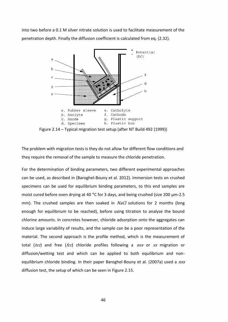
46
into two before a 0.1 M silver nitrate solution is used to facilitate measurement of the
penetration depth. Finally the diffusion coefficient is calculated from eq. (2.32).
Figure 2.14 – Typical migration test setup (after NT Build 492 (1999))
The problem with migration tests is they do not allow for different flow conditions and
they require the removal of the sample to measure the chloride penetration.
For the determination of binding parameters, two different experimental approaches
can be used, as described in (Baroghel-Bouny et al. 2012). Immersion tests on crushed
specimens can be used for equilibrium binding parameters, to this end samples are
moist cured before oven drying at 40 °C for 3 days, and being crushed (size 200 μm-2.5
mm). The crushed samples are then soaked in NaCl solutions for 2 months (long
enough for equilibrium to be reached), before using titration to analyse the bound
chlorine amounts. In concretes however, chloride adsorption onto the aggregates can
induce large variability of results, and the sample can be a poor representation of the
material. The second approach is the profile method, which is the measurement of
total (tcc) and free (fcc) chloride profiles following a nss or ss migration or
diffusion/wetting test and which can be applied to both equilibrium and non-
equilibrium chloride binding. In their paper Baroghel-Bouny et al. (2007a) used a nss
diffusion test, the setup of which can be seen in Figure 2.15.
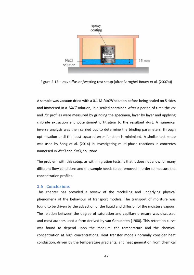
47
Figure 2.15 – nss diffusion/wetting test setup (after Baroghel-Bouny et al. (2007a))
A sample was vacuum dried with a 0.1 M NaOH solution before being sealed on 5 sides
and immersed in a NaCl solution, in a sealed container. After a period of time the tcc
and fcc profiles were measured by grinding the specimen, layer by layer and applying
chloride extraction and potentiometric titration to the resultant dust. A numerical
inverse analysis was then carried out to determine the binding parameters, through
optimisation until the least squared error function is minimised. A similar test setup
was used by Song et al. (2014) in investigating multi-phase reactions in concretes
immersed in NaCl and CaCl2 solutions.
The problem with this setup, as with migration tests, is that it does not allow for many
different flow conditions and the sample needs to be removed in order to measure the
concentration profiles.
2.6 Conclusions
This chapter has provided a review of the modelling and underlying physical
phenomena of the behaviour of transport models. The transport of moisture was
found to be driven by the advection of the liquid and diffusion of the moisture vapour.
The relation between the degree of saturation and capillary pressure was discussed
and most authors used a form derived by van Genuchten (1980). This retention curve
was found to depend upon the medium, the temperature and the chemical
concentration at high concentrations. Heat transfer models normally consider heat
conduction, driven by the temperature gradients, and heat generation from chemical

48
reactions. The transport of a chemical ion is assumed to be driven by liquid advection,
mechanical dispersion and diffusion of the ions, where the diffusion is coupled through
an electrical potential term, described by Poisson’s equation, to prevent the break-up
of electro neutrality. The chemical reactions were also considered including the
reaction classes which affect the mathematical treatment of the reaction. In this case,
the kinetic reactions were assumed to be described by a Freundlich isotherm, where
the reaction rate is driven by the chemical concentration or solution supersaturation.
Different methods for calculating ion activity were discussed, where the Pitzer model is
preferred for higher concentrations due to its greater range of applicability.
A review of coupled models found in the literature for modelling transport was made
including a review of the approaches to increasing the efficiency of their solution. It
was found that there are two schools of thought with regard to this; one uses operator
splitting approaches whilst the other employs reformulation techniques. It was found,
however, that operator splitting techniques can introduce errors or have convergence
problems and reformulation techniques are limited in the amount of reduction that
can be achieved (i.e. overall reduction in the number of coupled equations to be
solved), depending on the chemical system. It was therefore concluded that there is a
need for a new set of efficient reduction approaches that can be applied –without
modification- to a range of chemical systems.
Finally a review of the current approaches to determining transport parameters was
made, including those applied to both soils and cementitious materials. It was found
that there were a number of drawbacks with current approaches for cementitious
materials, including the inability to allow for different flow conditions and the
requirement of the removal of the sample for concentration measurements. It is
therefore concluded that there is a need for a new approach to determining transport
parameters in cementitious materials that allows for different flow conditions and the
in situ measurement of concentrations.
49
Chapter 3. Theoretical Formulation
3.1 Introduction
This chapter presents the theoretical formulation of the governing equations
describing mass and energy balance and physical laws describing the various physical
processes considered. The primary variables considered here are the capillary pressure
(PC), the temperature (T) and the dissolved chemical concentration (ci) of each species.
Section 3.2 describes the governing equation for moisture transfer, which is split into
two parts; liquid moisture flux and moisture vapour flux. For each part the governing
equation of mass balance is presented and the various mechanisms of transport
including the advection, diffusion and phase change between the two described.
The enthalpy balance equation and mechanisms of heat transfer including conduction
is covered in section 3.3.
The theoretical formulation that describes the physical processes of ion transport will
then be presented in section 3.4 including the advection with the liquid phase,
hydrodynamic dispersion and the condition of charge neutrality based on the Nernst
Planck and Poisson equations considering the no current condition.
Section 3.5 is dedicated to the description of the chemical reactions that may take
place. The chemical reactions presented are considered as non-equilibrium reactions
described with a Freundlich type isotherm. Following this, the calculation of ion
activity, used at times in the place of concentration for reaction rates, using the Pitzer
equations is discussed.
Finally, in section 3.6, the chapter is summarised.
3.2 Moisture Flow
The flow of moisture in porous materials is considered to be composed of two main
transfer mechanisms, the advection of the liquid water and the diffusion of the
moisture vapour. The governing mass balance equations for each will be derived
below.
50
3.2.1 Governing Equation for Moisture Flow
The mass balance equation considered here is the macroscopic volume averaged
balance equation, which for a phase π has the general form (Hassanizadeh and Gray
1979), (full details of the averaging procedure can be found in (Hassanizadeh and Gray
1979; Lewis and Schrefler 1998)), can be expressed as:
( ) (3.1)
where is the phase averaged density, is the mass averaged velocity, iπ is the
surface flux vector, is the phase averaged external supply of mass π, is the
phase averaged production, is the mass change between phases, and the superior
dot indicates the time derivative. The phase averaged density is given by:
(3.2)
where denotes the average density of phase π, n denotes the porosity of the
medium and Sπ denotes the degree of saturation of phase π. Assuming iπ, and
are all equal to zero the mass balance equation for liquid moisture is given by:
( ) (3.3)
where denotes the rate of phase change between liquid moisture and moisture
vapour. The gaseous phase consists of dry-air and moisture vapour, which are miscible
and so following (Lewis and Schrefler 1998) are assumed to have the same volume
fraction Sg the mass balance equations for dry-air and moisture vapour are given as:
( ) (3.4)
( ) (3.5)
However, the mass balance of dry-air is neglected here following Bary et al. (2008) and
de Morais et al. (2009), who found that a model based on the assumption that the gas
phase consisted of moisture vapour only was able to accurately capture the moisture
transport behaviour when compared to results of a full model, while reducing the
computational cost of the simulation. The assumption used here is that the combined
gas pressure of moisture vapour and dry-air remains constant at atmospheric pressure,
51
following the approach of Chitez and Jefferson (2015). This is justified as Gardner et al.
(2008) found that the time to reach steady state of the gas flow is relatively short and
so any excess pressures would be negligible in all but short time scales. Introducing a
diffusive dispersive flux Jv for the moisture vapour gives:
( ) (3.6)
3.2.2 Mechanisms of Liquid Moisture Transport
The velocity of the liquid moisture phase is given by a generalised form of Darcy’s law
(Gawin et al. 2006), which is given as:
( ) (3.7)
where Ki is the intrinsic permeability of the medium, Krw is the relative permeability of
the liquid moisture phase, μw is the dynamic viscosity of water, is the gravity vector
and Pw is the liquid pressure. The capillary pressure is the chosen primary variable for
the moisture phase, following the approach of Gawin et al. (2006). The capillary
pressure, PC, arises as a result of the interfacial tension between the liquid and gas
phases and is defined as the difference between the gas pressure, Pg, and liquid
pressure and can be expressed as:
(3.8)
Following Dalton’s law of partial pressures this gives the combined pressure of dry-air
and moisture vapour to be equal to atmospheric:
(3.9)
Noting eq. (3.8), eq. (3.7) can be rewritten as:
( ) (3.10)
as the gas pressure is assumed to be constant then the first term in the bracket of eq.
(3.10) is equal to zero giving:
( ) (3.11)
52
The capillary pressure can be linked to the external relative humidity (RH) through the
Kelvin equation (Gawin et al. 2006) given as:
(
)
( ) (3.12)
where R is the ideal gas constant, T is the temperature, Mw is the molar mass of water,
Pv is the vapour pressure and Pvs is the saturated vapour pressure which is related to
the saturated vapour density through the ideal gas law (Gawin et al. 2006), which is
given for a phase π as:
(3.13)
and is a function of temperature and is given by Antione’s equation as:
(3.14)
where b1-5 are material parameters. The moisture density ρw depends on temperature,
and the relationship proposed by McCutcheon (1993) is considered here:
[ ( ) ( )
( )] (3.15)
where a1-5 are material parameters.
The remaining terms from eq. (3.7), as yet undefined, are the relative permeability of
the medium Krw and the dynamic viscosity of water μw and these are considered in the
following paragraph. The dynamic viscosity has been reported to depend on both the
temperature and solute concentration (Gawin et al. 1999; Koniorczyk 2010) and is
given by:
( ∑
(∑
)
(∑
)
) ( )
(3.16)
where A1-3 are material parameters, is the chemical concentration of a species i and
ns is the number of chemical species. The intrinsic permeability is reported to depend
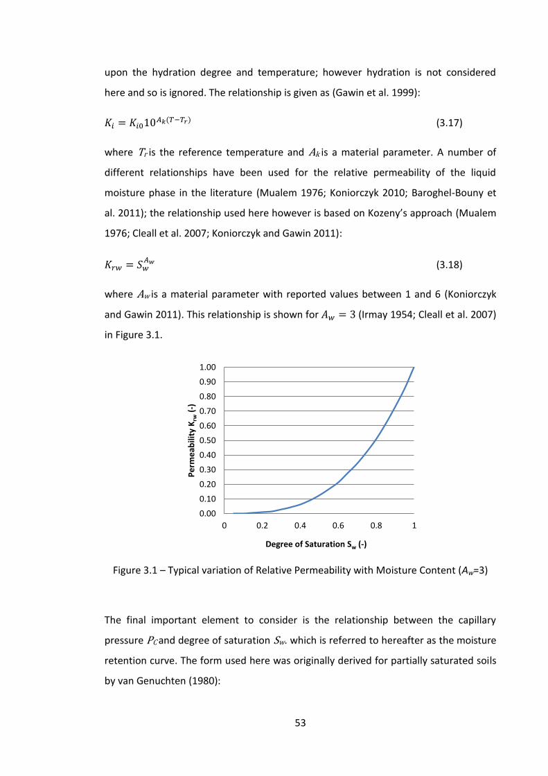
53
upon the hydration degree and temperature; however hydration is not considered
here and so is ignored. The relationship is given as (Gawin et al. 1999):
( ) (3.17)
where Tr is the reference temperature and Ak is a material parameter. A number of
different relationships have been used for the relative permeability of the liquid
moisture phase in the literature (Mualem 1976; Koniorczyk 2010; Baroghel-Bouny et
al. 2011); the relationship used here however is based on Kozeny’s approach (Mualem
1976; Cleall et al. 2007; Koniorczyk and Gawin 2011):
(3.18)
where Aw is a material parameter with reported values between 1 and 6 (Koniorczyk
and Gawin 2011). This relationship is shown for (Irmay 1954; Cleall et al. 2007)
in Figure 3.1.
Figure 3.1 – Typical variation of Relative Permeability with Moisture Content (Aw=3)
The final important element to consider is the relationship between the capillary
pressure PC and degree of saturation Sw. which is referred to hereafter as the moisture
retention curve. The form used here was originally derived for partially saturated soils
by van Genuchten (1980):
0.00
0.10
0.20
0.30
0.40
0.50
0.60
0.70
0.80
0.90
1.00
0 0.2 0.4 0.6 0.8 1
Pe
rme
abili
ty K
rw (
-)
Degree of Saturation Sw (-)
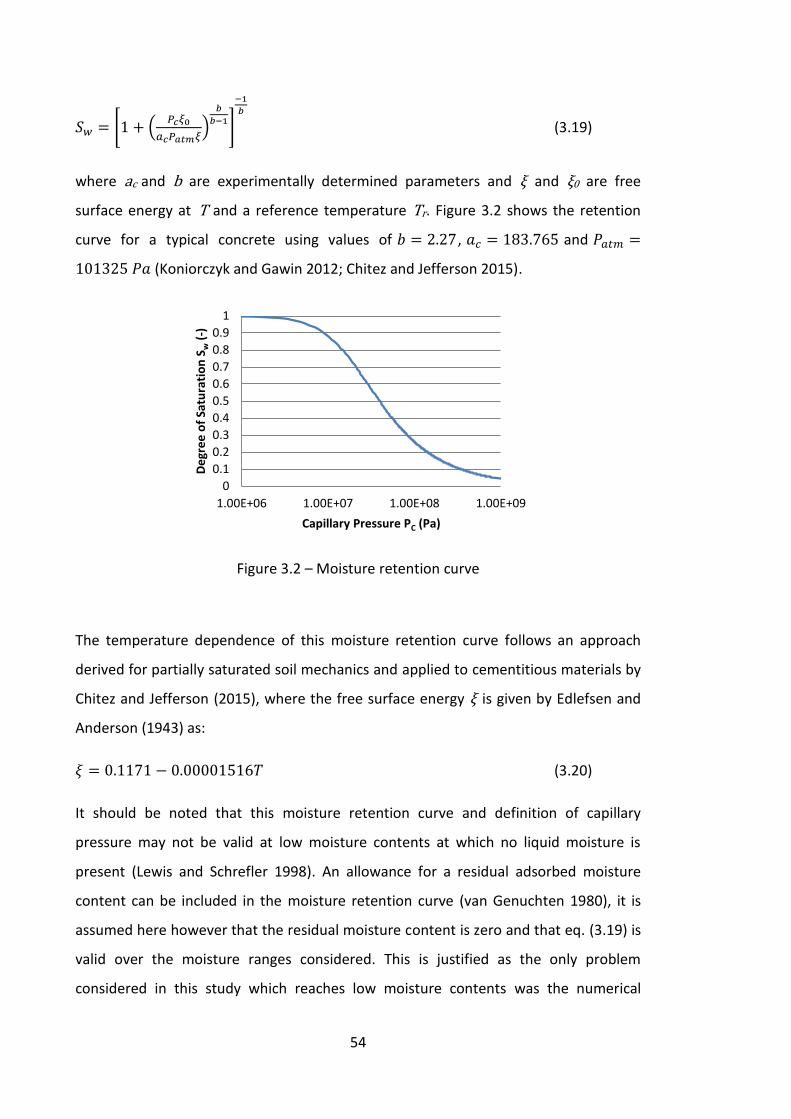
54
[ (
)
]
(3.19)
where ac and b are experimentally determined parameters and ξ and ξ0 are free
surface energy at T and a reference temperature Tr. Figure 3.2 shows the retention
curve for a typical concrete using values of , and
(Koniorczyk and Gawin 2012; Chitez and Jefferson 2015).
Figure 3.2 – Moisture retention curve
The temperature dependence of this moisture retention curve follows an approach
derived for partially saturated soil mechanics and applied to cementitious materials by
Chitez and Jefferson (2015), where the free surface energy ξ is given by Edlefsen and
Anderson (1943) as:
(3.20)
It should be noted that this moisture retention curve and definition of capillary
pressure may not be valid at low moisture contents at which no liquid moisture is
present (Lewis and Schrefler 1998). An allowance for a residual adsorbed moisture
content can be included in the moisture retention curve (van Genuchten 1980), it is
assumed here however that the residual moisture content is zero and that eq. (3.19) is
valid over the moisture ranges considered. This is justified as the only problem
considered in this study which reaches low moisture contents was the numerical
0
0.1
0.2
0.3
0.4
0.5
0.6
0.7
0.8
0.9
1
1.00E+06 1.00E+07 1.00E+08 1.00E+09
De
gre
e o
f Sa
tura
tio
n S
w (
-)
Capillary Pressure PC (Pa)
55
experiment found in Koniorczyk (2010), which did not take this phenomenon into
account.
3.2.3 Mechanisms of Water Vapour Transport
The velocity of the moisture vapour phase is given by generalised Darcy’s law (Gawin
et al. 2006) given as:
( ) (3.21)
where Krg is the relative permeability of the gas phase, μg is the dynamic viscosity of
the gas, and Pg is the gas pressure. It is assumed in this thesis however as previously
mentioned that the gas pressure remains constant at atmospheric pressure, following
the approach of Chitez and Jefferson (2015). The first term in the bracket in (eq. 3.21)
therefore is zero. In addition to this the advection of the moisture vapour due to
gravity is also neglected here following the approach of previous authors (Gawin et al.
1999; de Morais et al. 2009). The advection of moisture vapour therefore is neglected
in this thesis, meaning that the main transport mechanism for moisture vapour
considered is the diffusion of the moisture vapour through the gas phase. This diffusive
flux is assumed to follow Fick’s law (Gawin et al. 2006) and is given by:
(
) (3.22)
taking into account the assumption that Pg=Patm and converting the gas density to gas
pressure through the ideal gas law eq. (3.13), eq. (3.22) becomes:
(3.23)
where Dm is the effective moisture vapour diffusivity which following (Gawin et al.
1999) is given by:
( ) (
)
(3.24)
where Av and Bv are material parameters, fs is a factor to take into account the
Knudsen effect and Dv0 is the free air diffusivity. Equation (3.23) can be simplified to:
56
(3.25)
where the moisture vapour diffusivity is given as:
(3.26)
3.3 Heat Flow
The energy balance equation that governs heat flow is given as:
( ) ∑
(3.27)
where is the heat capacity, Jq the heat flux, and
represent the latent
heat of vaporisation and the heat generated by chemical reactions respectively and nr
represents the number of chemical reactions.
The heat capacity is given as (Koniorczyk 2010):
( ) ( ) ( ) ∑
(3.28)
where Cπ represents the specific heat of phase π, with the s subscript representing the
solid matrix, the p subscript the precipitated or sorbed material and is the initial
porosity of the medium.
The third term in eq. (3.27), the heat flux represents heat conduction which is assumed
to follow Fourier’s law and is given by (Gawin et al. 2006):
(3.29)
where kt is the thermal conductivity of the medium which depends on temperature,
void ratio and degree of saturation following (Gawin et al. 1999) and can be defined as:
[ ( )] [
( ) ] (3.30)
where kt0 and Aλ are material parameters.
The remaining term to be defined in eq. (3.27) is the second term which represents the
convective heat transfer. It is assumed in this thesis however following de Morais et al.
57
(2009), Davie et al. (2010) and Gawin et al. (2011a; 2011b) that this term can be
neglected with little loss of accuracy and so it is ignored hereafter.
3.4 Ion Transport
The mass balance equation that governs the transport of a solute within the liquid
moisture phase is given as:
( )
(3.31)
where Jd represents the chemical flux and the final term on the left hand side
represents any sources/sinks due to chemical reactions and is discussed in more detail
in the following section. The second term in eq. (3.31) represents the advection of the
solute which is driven by the liquid moisture velocity and has been discussed in the
previous section. The third term represents the flux of the solute; this represents the
hydrodynamic dispersion of the solute and is given as (Koniorczyk 2010):
(3.32)
where is the diffusive flux of species i and
is the coefficient of mechanical
dispersion, which can be described following Bear and Bachmat (1990) as:
| | ( )
| |, {
(3.33)
where and are the transverse and longitudinal dispersivities.
An important consideration in the transport of chemical species is the charge
neutrality condition (Lasaga 1981; Baroghel-Bouny et al. 2011; Song et al. 2014). Pore
solutions tend towards being charge neutral as any areas of net charge would attract
ions of the opposite charge until the solution was balanced. If ions of opposite charge
were transported at different rates the charge of the solution could become
unbalanced, this leads to the development of an electric field that acts to balance the
diffusive flux of the ions and is described by the Poisson and Nernst-Planck equations
(Lasaga 1981; Baroghel-Bouny et al. 2011; Song et al. 2014):
(
) (3.34)
58
[∑ (| | | | ) ] (3.35)
where is the molecular diffusion coefficient of a positively or negatively charged
ion i, z is the charge of an ion, F is Faraday’s constant, is the electrical potential, ρ is
the charge density, ns is the number of chemical species and is the dielectric
permittivity of the liquid phase. The first term in eq. (3.35) is often small with
comparison to the second and ρ can be taken as zero following (Song et al. 2014),
reducing the Poisson equation to:
∑ (| | | | ) (3.36)
If the initial pore solution in the medium is initially neutral then eq. (3.36) means that
the current in the medium should be zero giving the diffusion of the ion i as:
( ∑
∑
∑
∑
) (3.37)
Taking this into account the total flux of an ion i can be given by:
(
∑ ∑
∑
∑
)
(3.38)
3.5 Chemical Reactions
The chemical reactions considered throughout this thesis are class 5 (‘insufficiently fast
surface’) or class 6 (‘insufficiently fast classical’) reactions (Rubin 1983) following the
scope of this thesis. The term ‘insufficiently fast’ means that the rate of transport of
the ions is faster than the rates of reaction, such that the local equilibrium assumption
is not valid. The terms ‘surface’ and ‘classical’ refer to adsorption/desorption and
precipitation/dissolution reactions respectively. The reaction rates are considered in
two ways here, empirical rates based on the literature (eq. 3.39) and reaction rates
based on a combination of empirical values and the activity of the ions in the solution
(eqs. 3.40 & 3.41). The first type considered based on empirical rates use a Freundlich
type description (Baroghel-Bouny et al. 2011; Song et al. 2014) of the general form:
59
(3.39)
where kd and ka are the desorption and adsorption (or dissolution and precipitation)
rates respectively, and λ is the order of the reaction. A plot of a typical Freundlich
isotherms for three different reaction orders is shown in Figure 3.3 assuming
and .
Figure 3.3 – Rate of reaction as calculated by Freundlich isotherm
The calculation of the activity of ions is undertaken in order to take into account the
deviation of the solution from an ideal solution. This deviation arises from the fact that
the charge of the ions affects their distribution within the solvent, with ions of like
charges repelling each other and opposite attracting; meaning that they are not
randomly distributed throughout the solvent. The reactions which consider the activity
of the solution have a similar form to eq. (3.39) and are also based on a Freundlich
type description which is given for precipitation and dissolution (or adsorption and
desorption) by Koniorczyk (2012):
( ) ,
(3.40)
| | ,
(3.41)
0
0.05
0.1
0.15
0.2
0.25
0 0.1 0.2 0.3 0.4 0.5
Rat
e o
f R
eac
tio
n d
S p (
s-1)
Chemical Concentration (kg/kg)
λ=2
λ=3
λ=4
60
where kda is a reaction rate, A’ is a constant which depends on the reaction and porous
medium and is the solution supersaturation ratio which is given as the quotient of
the solution activity , and the equilibrium constant for the considered reaction K:
(3.42)
The Pitzer equations are used here to calculate the activity coefficient of the ions
(Pitzer 1973; Steiger et al. 2008; Koniorczyk 2012), which is an extension of Debye-
Hückel Theory. The Debye-Hückel equation calculates the activity coefficient of the
solution based on the ionic strength of the solution whereas the Pitzer equations also
take into account the binary interactions of individual ions and can include higher
terms for interaction between three ions and more. The extended Debye-Hückel
theory is valid for concentrations up to 0.1 M (Koniorczyk 2012) whereas the Pitzer
equations are valid to 6 M for certain ions (Pitzer and Mayorga 1973). The activity
coefficients for an anion m and a cation x as predicted by the Pitzer equations are
given as:
( ) | | (3.43)
( ) | | (3.44)
where , and are the activity coefficient, charge and mass respectively for an
anion or cation, and are the second and third virial coefficients, Z is a function
given as:
∑ | | (3.45)
and is a function which depends on the ionic strength given as:
[
( )]
(3.46)
where is the Debye-Hückel parameter for the osmotic coefficient, b is a universal
parameter and I is the ionic strength of the solution given as:
∑
(3.47)
The second virial coefficients found in eq. (3.43) and eq. (3.44) are given as:
61
(3.48)
( )
( ) (3.49)
(
)
(
)
(3.50)
where and are parameters depending on the type of electrolyte and and
are functions given as:
( )
( ( ) ) (3.51)
( )
( ( ) ) (3.52)
The third virial coefficient is given as:
| | (3.53)
The coefficients in eqs. (3.48, 3.49, 3.50 & 3.53) depend on the temperature and
pressure and are given by:
( ) (
) (
) ( ) (
) ( )
(3.54)
where q1-6 are experimentally determined parameters. Given the activity coefficients
the activity of any salt can be calculated by:
(3.55)
where aw is the activity of water which can be calculated from:
(∑ ) (3.56)
where is the osmotic coefficient of the solution and is given as:
∑ [
(
)] (3.57)
An example of how the chemical activity varies with chemical concentration can be
seen in Figure 3.4 (Koniorczyk 2012).
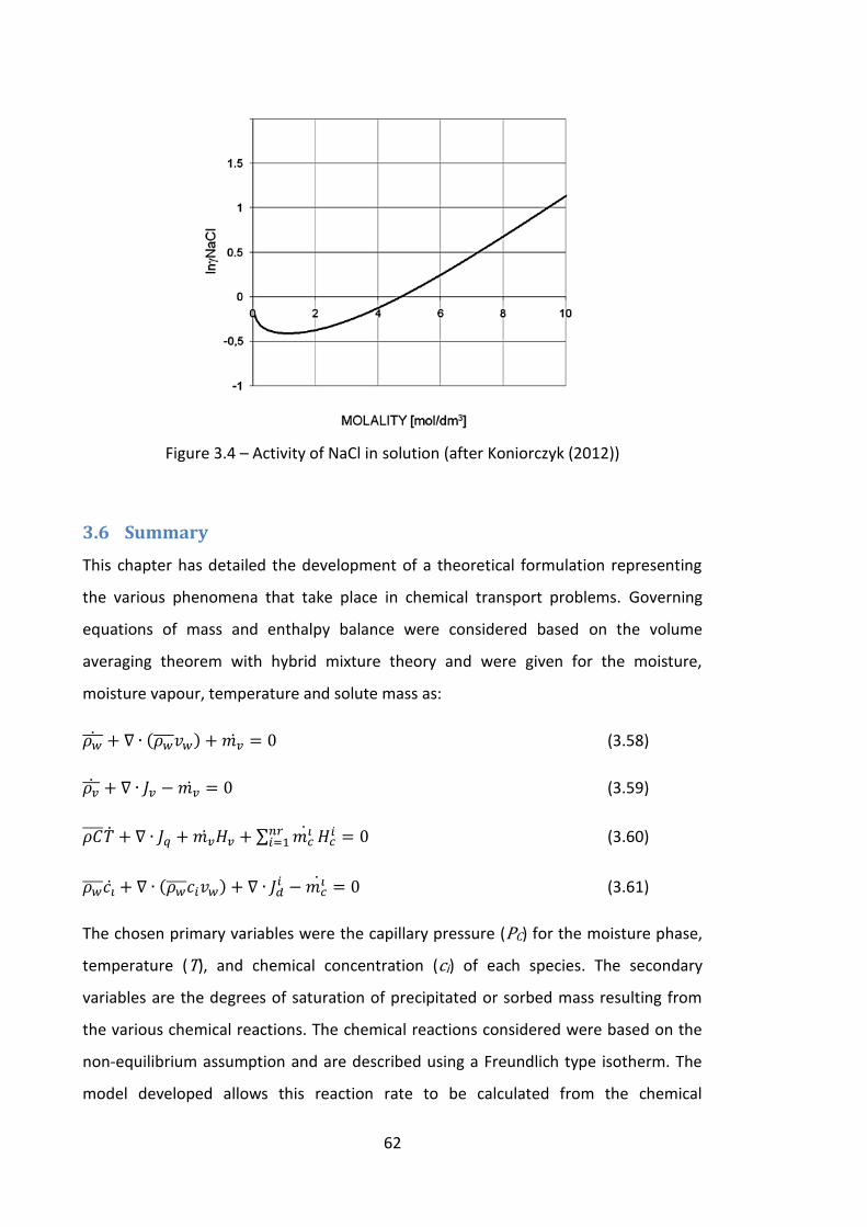
62
Figure 3.4 – Activity of NaCl in solution (after Koniorczyk (2012))
3.6 Summary
This chapter has detailed the development of a theoretical formulation representing
the various phenomena that take place in chemical transport problems. Governing
equations of mass and enthalpy balance were considered based on the volume
averaging theorem with hybrid mixture theory and were given for the moisture,
moisture vapour, temperature and solute mass as:
( ) (3.58)
(3.59)
∑
(3.60)
( )
(3.61)
The chosen primary variables were the capillary pressure (PC) for the moisture phase,
temperature (T), and chemical concentration (ci) of each species. The secondary
variables are the degrees of saturation of precipitated or sorbed mass resulting from
the various chemical reactions. The chemical reactions considered were based on the
non-equilibrium assumption and are described using a Freundlich type isotherm. The
model developed allows this reaction rate to be calculated from the chemical

63
concentrations, or for concentrated solutions the ion activities. For the ion activities
the Pitzer model was chosen following the approach by Koniorczyk (2012) for its ability
to accurately predict the activities at higher concentrations than Debye-Hückel type
theories allow.

64
65
Chapter 4. Numerical Formulation
4.1 Introduction
The previous chapter presented the theoretical formulation of both the governing
equations of mass and energy balance and the constitutive equations describing the
physical phenomena. This chapter details the derivation of a numerical procedure used
for the solution of the governing system of equations. This type of equation system is
usually dealt with using a coupled solution procedure due to the strong
interdependence of the primary variables (for example the dependence of solute
transport on the liquid moisture advection, which in turn depends on the solute
concentration through the liquid density and in some cases viscosity).
The finite element method (FEM) is chosen for the spatial discretisation of the system,
where the Galerkin method was employed for choice of the weighting functions. An
implicit Euler backward difference scheme was chosen for the temporal discretisation,
before finally a Newton-Raphson iteration procedure is employed to solve the system
of nonlinear equations. Section 4.2 begins with the formulation of the boundary value
problem, before providing a brief explanation of the approach of the FEM and the
choice of the weighting functions in section 4.3. The temporal discretisation is detailed
in section 4.4 along with the description of the Newton-Raphson procedure.
The model was implemented in FORTRAN and was developed from the starting point
of a linear elastic FORTRAN code, written to the coding standard of the research group.
One of the aims of the research of this thesis is to develop a numerical reduction
scheme to reduce the computational cost of simulations, whilst maintaining suitable
accuracy. Three reduction techniques are proposed each of which reduces the number
of chemical species considered in the global system of equations, by calculating the
transport of only a number of indicator species (up to 3 depending on the particular
technique). The transport of the non-indicator species is then calculated at the end of
a time step as a function of the transport of the indicator species. The description of
these techniques is presented in section 4.5, before finally a summary of the numerical
approach is made in section 4.6.
66
4.2 Formulation of Boundary Value Problem
The governing equations of mass and energy balance presented in Chapter 3 (from
eqs. 3.58, 3.59, 3.60 & 3.61) for the liquid moisture, moisture vapour, temperature and
chemical species are recalled here, as follows:
( ) (4.1)
(4.2)
∑
(4.3)
( )
(4.4)
Summing together eq. (4.1) and eq. (4.2) to give the total moisture mass balance
equation results in:
( ) (4.5)
and rearranging eq. (4.1) to give the value of the rate of mass change from liquid to
vapour, gives:
( ) (4.6)
this can then be substituted into the enthalpy balance equation (eq. 4.3) to give:
( ( )) ∑
(4.7)
this gives the governing system of equations to be solved for the principal variables PC,
T and c as:
( ) (4.8)
( ( )) ∑
(4.9)
( )
(4.10)
subject to (i) initial conditions which specify the values of the primary variables at the
beginning of the analysis of:
(4.11)
67
(ii) the Dirichlet boundary conditions of:
( ) (4.12)
( ) (4.13)
( ) (4.14)
and (iii) the Cauchy type boundary conditions given as:
( ) ( ) (4.15)
( ) ( ) (4.16)
( ) (
) (4.17)
where is the unit normal vector to the boundary , qwv, qt and qc are the applied
moisture, heat and chemical fluxes respectively and , and are the convective
boundary transfer coefficients for moisture, heat and chemical species respectively.
, and
are the environmental values of moisture vapour density,
temperature and chemical concentration respectively.
4.3 Finite Element Solution
4.3.1 General Solution
The next step is to apply the spatial discretisation of the above system. In this thesis,
the finite element method is chosen for this following the approach of many other
authors (Lewis and Schrefler 1998; Gawin et al. 2006; Cleall et al. 2007; Koniorczyk
2012; Thomas et al. 2012; Chitez and Jefferson 2016). A brief description of the finite
element method will be presented here; however, for full details refer to Zienkiewicz
et al. (2013). To demonstrate the finite element approach we can consider a general
boundary value problem of the form:
( ) (4.18)
( ) (4.19)
68
in which A and B are arbitrary differential operators. Integrating over the domain and
boundary we can make the following statement:
∫ ( )
∫ ( )
(4.20)
where W is an arbitrary weighting function. Assuming that the integrands can be
evaluated there are some restrictions on the choice of functions for W, full details of
which can be found in (Zienkiewicz et al. 2013). Once the equations are set in this form
we can apply the integral over a number of finite elements, which are summed
together to form the global discretised system:
∫ ( )
∫ ( )
∑ (∫ ( ) ∫ ( )
) (4.21)
noting that the finite element method is an approximation method the solution will be
of the form:
∑ (4.22)
where N is a vector of shape functions defined in terms of local coordinates in section
4.3.4. From this we then obtain the weighted residual equation:
∑ (∫ ( ) ∫ ( )
) (4.23)
where ( ) and ( ) represent the residual error and the boundary residual error
respectively that arise from the approximation (eq. 4.22). The approach of the finite
element method is to minimise this residual.
4.3.2 Application to the System of Governing Equations
Applying the above discretisation to the governing equations of mass and energy
balance (eqs. 4.3, 4.4 & 4.5) gives:
∫
( ( ) ) ∫ (( )
( )) (4.24)
∫
( ( ( )) ∑
) ∫ ((
) ( )) (4.25)
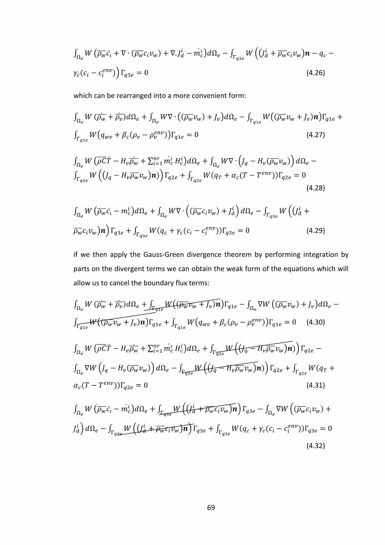
69
∫
( ( )
) ∫ (( )
( )) (4.26)
which can be rearranged into a more convenient form:
∫
( ) ∫
(( ) ) ∫ (( ) )
∫ ( ( ))
(4.27)
∫
( ∑
) ∫
( ( ))
∫ (( ) )) ∫ ( ( ))
(4.28)
∫
( ) ∫
(( )
) ∫ ((
) ) ∫ ( ( ))
(4.29)
if we then apply the Gauss-Green divergence theorem by performing integration by
parts on the divergent terms we can obtain the weak form of the equations which will
allow us to cancel the boundary flux terms:
∫
( ) ∫ (( ) ) ∫
(( ) )
∫ (( ) ) ∫ ( ( ))
(4.30)
∫
( ∑
) ∫ (( ) ))
∫
( ( )) ∫ (( ) )) ∫ (
( )) (4.31)
∫
( ) ∫ ((
) ) ∫
(( )
) ∫ ((
) ) ∫ ( (
))
(4.32)
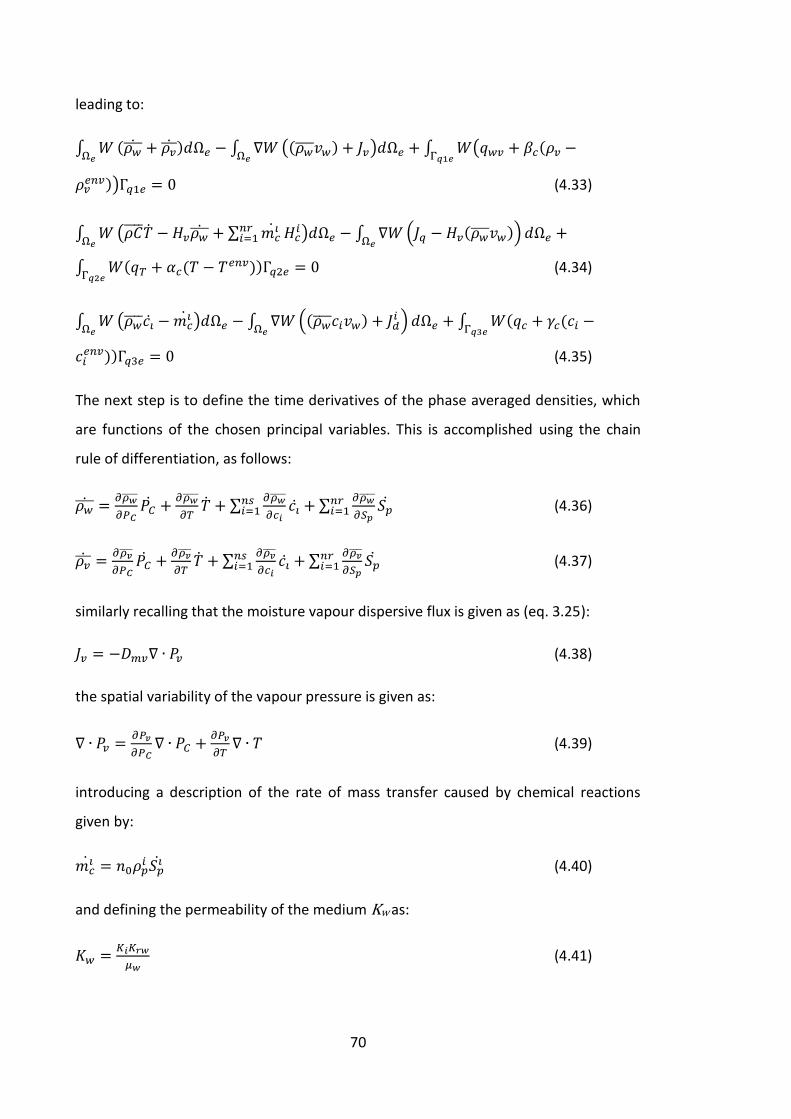
70
leading to:
∫
( ) ∫
(( ) ) ∫ ( (
)) (4.33)
∫
( ∑
) ∫
( ( ))
∫ ( ( )) (4.34)
∫
( ) ∫
(( )
) ∫ ( (
)) (4.35)
The next step is to define the time derivatives of the phase averaged densities, which
are functions of the chosen principal variables. This is accomplished using the chain
rule of differentiation, as follows:
∑
∑
(4.36)
∑
∑
(4.37)
similarly recalling that the moisture vapour dispersive flux is given as (eq. 3.25):
(4.38)
the spatial variability of the vapour pressure is given as:
(4.39)
introducing a description of the rate of mass transfer caused by chemical reactions
given by:
(4.40)
and defining the permeability of the medium Kw as:
(4.41)
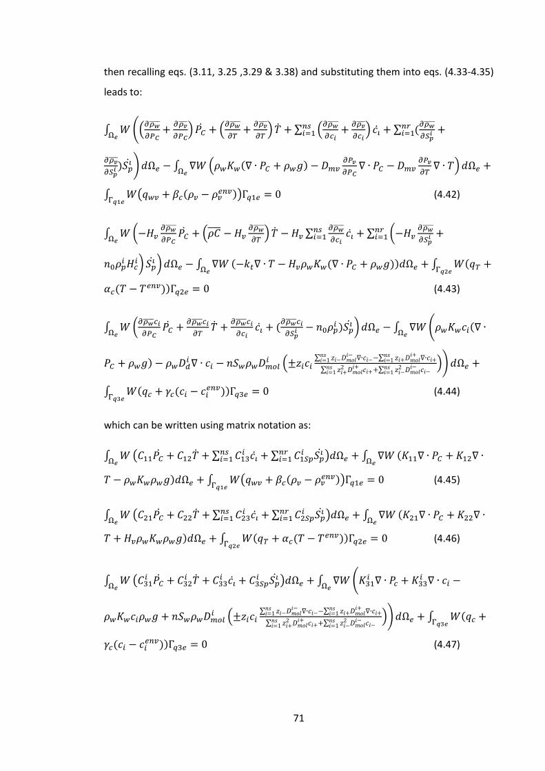
71
then recalling eqs. (3.11, 3.25 ,3.29 & 3.38) and substituting them into eqs. (4.33-4.35)
leads to:
∫
((
) (
) ∑ (
)
∑ (
)
) ∫
( ( )
)
∫ ( ( ))
(4.42)
∫
(
(
) ∑
∑ (
) ) ∫
( ( )) ∫ (
( )) (4.43)
∫
(
(
) ) ∫
( (
)
( ∑
∑
∑
∑
))
∫ ( ( ))
(4.44)
which can be written using matrix notation as:
∫
( ∑
∑
) ∫
(
) ∫ ( ( ))
(4.45)
∫
( ∑
∑
) ∫
(
) ∫ ( ( )) (4.46)
∫
(
) ∫
(
(
∑ ∑
∑
∑
)) ∫ (
( )) (4.47)
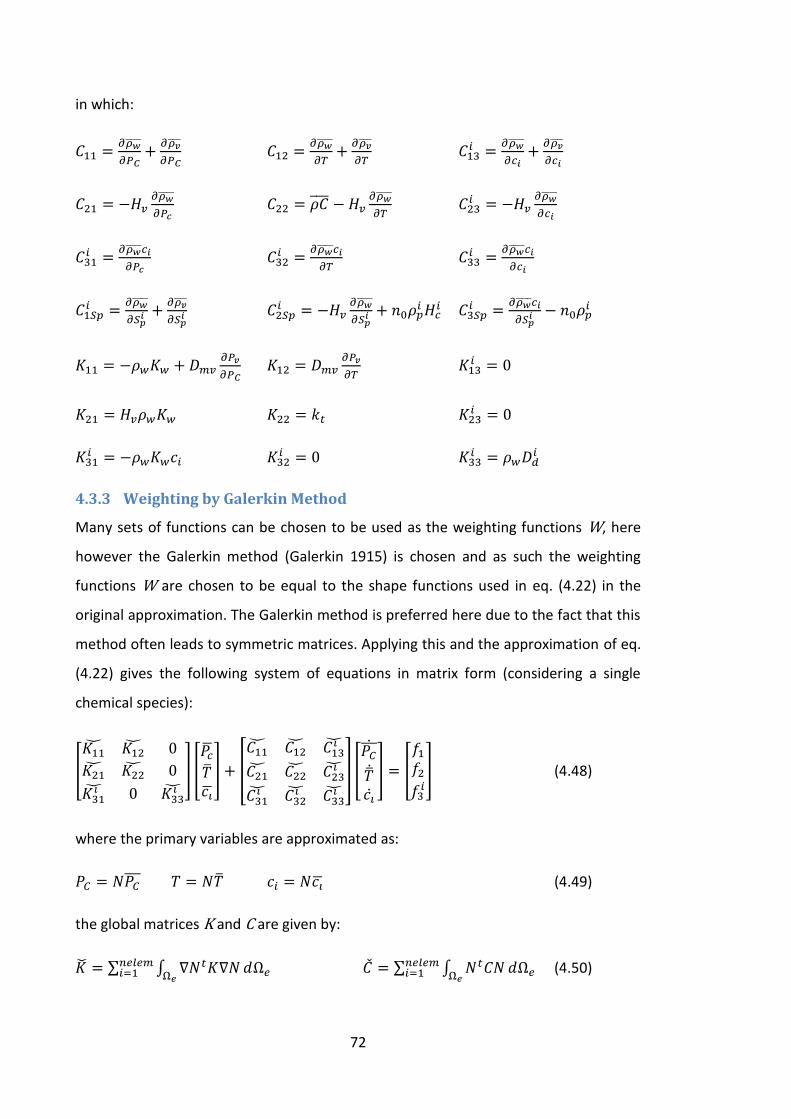
72
in which:
4.3.3 Weighting by Galerkin Method
Many sets of functions can be chosen to be used as the weighting functions W, here
however the Galerkin method (Galerkin 1915) is chosen and as such the weighting
functions W are chosen to be equal to the shape functions used in eq. (4.22) in the
original approximation. The Galerkin method is preferred here due to the fact that this
method often leads to symmetric matrices. Applying this and the approximation of eq.
(4.22) gives the following system of equations in matrix form (considering a single
chemical species):
[
] [
] [
] [
] [
] (4.48)
where the primary variables are approximated as:
(4.49)
the global matrices K and C are given by:
∑ ∫
∑ ∫
(4.50)
73
the global right hand side vector is given by:
∑ (4.51)
where the right hand side vector for each of the variables is given as:
∫
( ) ∫ ( ( ))
∫
(∑
) (4.52)
∫
( ) ∫ ( ( ))
∫
(∑
) (4.53)
∫
(
( ∑
∑
∑
∑
))
∫ ( ( ))
∫
(
) (4.54)
It can be seen in the chemical balance equation above that the flux term relating to the
charge neutrality condition has been moved to the right hand side, this is because here
it is to be dealt with explicitly. This global system of equations can be written in
condensed form as:
(4.55)
where is the vector of primary variables.
4.3.4 Shape Functions and Numerical Integration
As seen in the previous section, a vector of shape functions is used both in the
approximation of eq. (4.22) and through the choice of weighting functions. It is
therefore necessary to define these shape functions and describe the means of
evaluating the above integrals. Bilinear quadrilaterals are chosen here as the element
type, it can be noted however that other element types can be chosen depending on
the continuity required and on the geometry of the problem domain. The shape
functions of a bilinear quadrilateral are given as:
74
[ ( )( )
( )( )
( )( )
( )( )]
(4.56)
where and are local parametric coordinates with values range -1< , <+1, which
are mapped to the Cartesian coordinates using interpolation, known as isoparametric
mapping.
The integrals are evaluated in a numerical fashion using a Gauss-Legendre rule
(Zienkiewicz et al. 2013). The Gauss-Legendre method calculates the value of the
function at discrete points and sums them to give the approximation to the integral.
The 2x2 Gauss-Legendre rule is used here due to its ability to exactly evaluate the
integrals considered and due to convergence and stability criteria (Zienkiewicz et al.
2013). This rule uses 4 sampling points with local coordinates of (-1/3 , -1/3), (1/3 ,
-1/3), (1/3 , 1/3) and (-1/3 , 1/3), each with a weight of 1. Using this rule the
approximation of an integral I, is given by:
∫ ∫ ( , )
∑ ( , )
(4.57)
4.4 Temporal Discretisation and Non-linearity
Following the spatial discretisation of the last section, the next step is to carry out the
temporal discretisation. The method chosen here was the implicit backward difference
scheme following Gawin et al. (2006), which when applied to eq. (4.55) gives:
( ) (4.58)
equation (4.58) is non-linear as the matrices depend on the values of the primary
variables ; the error due to an approximation of these values is given by:
( ) (4.59)
To deal with this non-linearity the Newton-Raphson iteration procedure has been used
following Gawin et al. (2006), to minimise this approximation error. This approach
minimises this error by expanding eq. (4.59) as a Taylor’s series, ignoring higher order
terms and equating to zero, which gives:
75
[
]
(4.60)
which can be rearranged to give the change in primary variables :
[
]
( ) (4.61)
the iteration updates the primary variables as follows:
(4.62)
differentiating the error with respect to the primary variables and substituting into eq.
(4.59) gives the system of equations in matrix form:
{ [
] [
] [
]} [
] [
]
(4.63)
where K, C and are tangent matrices and are given by:
∑ ∫
∑ ∫
(4.64)
and:
, , ∑ ,
(4.65)
, , ∑ ,
(4.66)
The equations presented so far have been written for the consideration of one
chemical species, however this was just for brevity and the formulation remains the
same for two or more. The system of equations for ns chemical species would be given
as:
[
]
[
]
[
]
[
]
[
]
(4.67)
76
it can be noted here that in this thesis, since only kinetic reactions have been
considered, it is assumed that any coupling between chemical species can only be
found in the right hand side vector through the kinetic reaction rates and the charge
neutrality condition.
4.5 Problem Reduction Scheme
One of the main aims of this thesis is to address the computational demand posed by
certain reactive transport problems. In this section to reduce the size of the governing
system of equations three different reduction schemes, denoted PRS1, PRS2 and PRS3
are proposed and detailed. In each of these schemes, a reduced set of species is
chosen for full computation. These selected species are termed ‘indicators’ and the
response of the remaining species is computed at each time step based upon the
calculated transport of the indicators. The difference between the three reduction
approaches (PRS 1 to 3) lies in both the number of indicator species used and in the
method employed for calculating the transport of the remaining species.
The rate of transport of an ion depends on the moisture velocity (which is the same for
all ions), the concentration gradient and the diffusion coefficient. The three
approaches proposed here aim to estimate the transport of an ion relative to indicator
species, considering the differences in diffusion coefficient and the maximum
concentration gradient. For each PRS bounds checking was also implemented to
prevent physically meaningless results (i.e. negative concentrations).
4.5.1 PRS 1
The first reduction scheme is an extrapolation technique which uses just one indicator
species. The transport of all other species is computed from the incremental change in
the concentration of the indicator species multiplied by a concentration gradient ratio
and diffusion coefficient ratio, according to eq. (4.68). The concentration gradient
multiplier is the ratio of the maximum concentration gradients (initial concentration –
boundary concentration) of the current and indicator species respectively. The
diffusion coefficient ratio is defined in a similar manner. The concentration of a non-
indicator species i is given as:
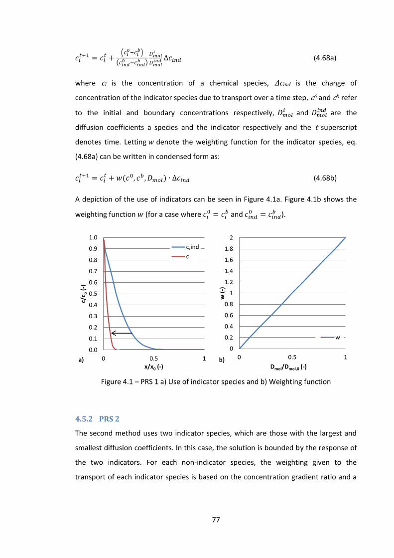
77
(
)
(
)
(4.68a)
where ci is the concentration of a chemical species, cind is the change of
concentration of the indicator species due to transport over a time step, c0 and cb refer
to the initial and boundary concentrations respectively, and
are the
diffusion coefficients a species and the indicator respectively and the t superscript
denotes time. Letting denote the weighting function for the indicator species, eq.
(4.68a) can be written in condensed form as:
( , , ) (4.68b)
A depiction of the use of indicators can be seen in Figure 4.1a. Figure 4.1b shows the
weighting function (for a case where
and
).
Figure 4.1 – PRS 1 a) Use of indicator species and b) Weighting function
4.5.2 PRS 2
The second method uses two indicator species, which are those with the largest and
smallest diffusion coefficients. In this case, the solution is bounded by the response of
the two indicators. For each non-indicator species, the weighting given to the
transport of each indicator species is based on the concentration gradient ratio and a
0.0
0.1
0.2
0.3
0.4
0.5
0.6
0.7
0.8
0.9
1.0
0 0.5 1
c/c o
(-)
x/x0 (-) a)
c,ind
c
0
0.2
0.4
0.6
0.8
1
1.2
1.4
1.6
1.8
2
0 0.5 1
w (
-)
Dmol/Dmol,0 (-) b)
w
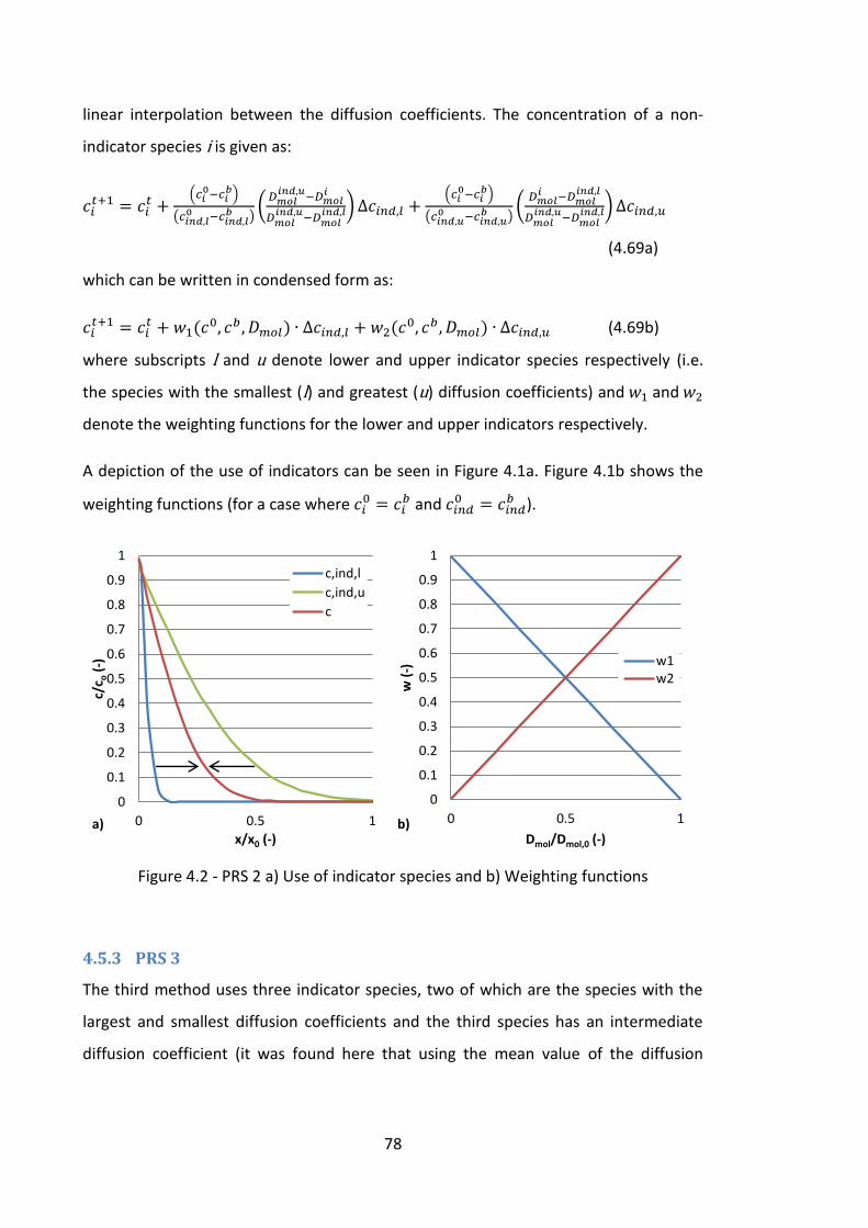
78
linear interpolation between the diffusion coefficients. The concentration of a non-
indicator species i is given as:
(
)
( , ,
)(
,
,
, ) , (
)
( , ,
)(
,
,
, ) ,
(4.69a)
which can be written in condensed form as:
( , , ) , (
, , ) , (4.69b)
where subscripts l and u denote lower and upper indicator species respectively (i.e.
the species with the smallest (l) and greatest (u) diffusion coefficients) and and
denote the weighting functions for the lower and upper indicators respectively.
A depiction of the use of indicators can be seen in Figure 4.1a. Figure 4.1b shows the
weighting functions (for a case where
and
).
Figure 4.2 - PRS 2 a) Use of indicator species and b) Weighting functions
4.5.3 PRS 3
The third method uses three indicator species, two of which are the species with the
largest and smallest diffusion coefficients and the third species has an intermediate
diffusion coefficient (it was found here that using the mean value of the diffusion
0
0.1
0.2
0.3
0.4
0.5
0.6
0.7
0.8
0.9
1
0 0.5 1
c/c o
(-)
x/x0 (-) a)
c,ind,l
c,ind,u
c
0
0.1
0.2
0.3
0.4
0.5
0.6
0.7
0.8
0.9
1
0 0.5 1
w (
-)
Dmol/Dmol,0 (-) b)
w1w2
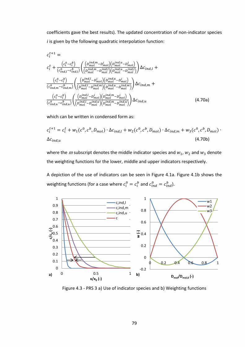
79
coefficients gave the best results). The updated concentration of non-indicator species
i is given by the following quadratic interpolation function:
(
)
( , ,
)(
( ,
)( ,
)
( ,
, )( ,
, )) ,
(
)
( , ,
)(
( ,
)( ,
)
( ,
, )( ,
, )) ,
(
)
( , ,
)(
( ,
)( ,
)
( ,
, )( ,
, )) , (4.70a)
which can be written in condensed form as:
( , , ) , (
, , ) , ( , , )
, (4.70b)
where the m subscript denotes the middle indicator species and , and denote
the weighting functions for the lower, middle and upper indicators respectively.
A depiction of the use of indicators can be seen in Figure 4.1a. Figure 4.1b shows the
weighting functions (for a case where
and
).
Figure 4.3 - PRS 3 a) Use of indicator species and b) Weighting functions
0
0.1
0.2
0.3
0.4
0.5
0.6
0.7
0.8
0.9
1
0 0.5 1
c/c o
(-)
x/x0 (-) a)
c,ind,lc,ind,mc,ind,uc
-0.2
0
0.2
0.4
0.6
0.8
1
0 0.2 0.4 0.6 0.8 1
w (
-)
Dmol/Dmol,0 (-) b)
w1w2w3
80
4.5.4 Boundary Conditions
The initial conditions for the PRS can be defined in the same way as the full model
using eq. (4.11). The boundary conditions for the PRSs are also defined in the same
way as the full model and should be of the same type for both ‘indicator’ and ‘non-
indicator’ species, with the latter being calculated on a point wise basis.
4.5.5 Charge Neutrality
Another key consideration is how the charge neutrality condition is dealt with for the
PRSs, since the transport of the non-indicator species is not calculated in the reduced
system of governing equations. To deal with this, the diffusive flux due to the electric
field is dealt with explicitly by using concentrations from the previous time step and
moving these to the right hand side of the governing equations in a similar manner to
the way that moisture flow under gravity is often included in transport computations.
For non-indicator species this can then be calculated on a point wise basis and
subtracted at the end of the PRS eqs. (4.68-4.70).
4.5.6 Chemical Reactions
The chemical reactions are considered in much the same way as in the full model with
the reaction rates being calculated using the most recent chemical concentrations and
moving them to the right hand side of the governing equations. For non-indicator
species they are calculated on a point wise basis and subtracted at the end of the PRS
eqs. (4.68-4.70).
A flow chart showing the pseudo-code of the algorithm of the solution procedure can
be seen in Figure 4.4.
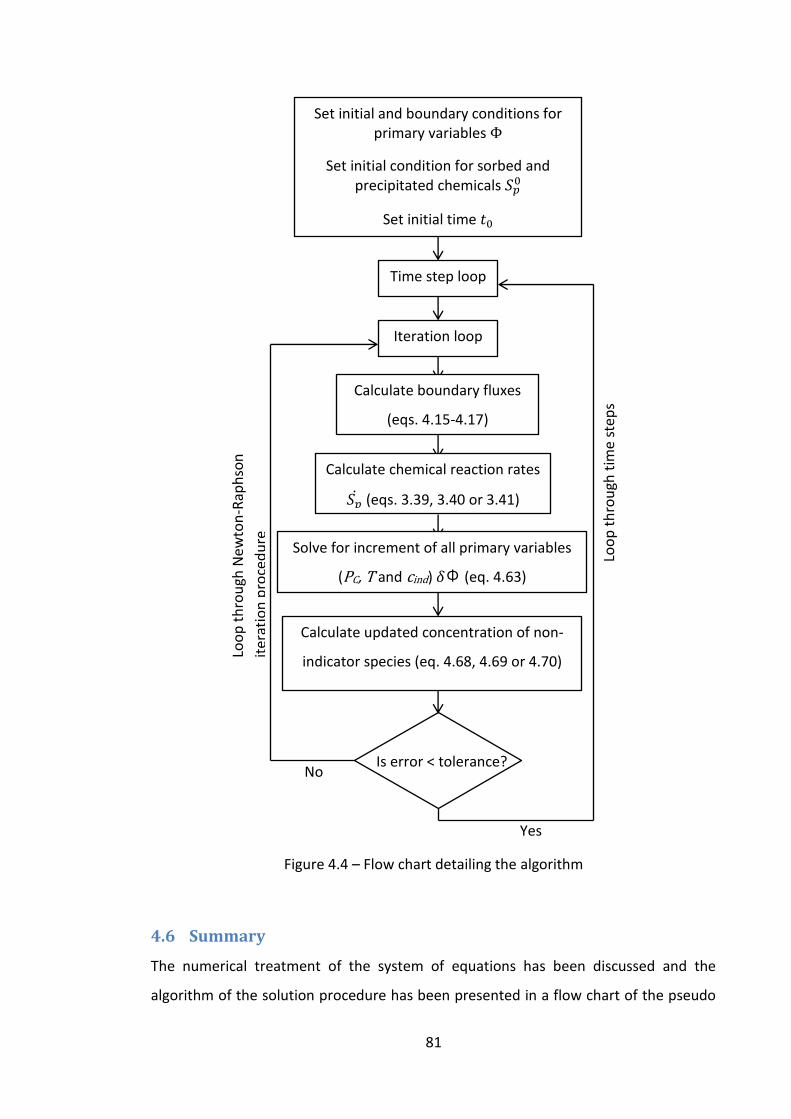
81
Figure 4.4 – Flow chart detailing the algorithm
4.6 Summary
The numerical treatment of the system of equations has been discussed and the
algorithm of the solution procedure has been presented in a flow chart of the pseudo
Set initial and boundary conditions for primary variables Φ
Set initial condition for sorbed and precipitated chemicals 𝑆𝑝
Set initial time 𝑡
Time step loop
Iteration loop
Calculate boundary fluxes
(eqs. 4.15-4.17)
Calculate chemical reaction rates
𝑆�� (eqs. 3.39, 3.40 or 3.41)
Solve for increment of all primary variables
(PC, T and cind) 𝛿Φ (eq. 4.63)
Is error < tolerance? No
Yes
Loo
p t
hro
ugh
tim
e st
eps
Loo
p t
hro
ugh
New
ton
-Rap
hso
n
iter
atio
n p
roce
du
re
Calculate updated concentration of non-
indicator species (eq. 4.68, 4.69 or 4.70)
82
code. The system of equations are treated as fully coupled and a numerical solution
using the FEM for the spatial discretisation and an implicit backward difference
method for the temporal discretisation has been developed. The nonlinearity of the
system is dealt with using a Newton-Raphson iteration procedure which used the
truncated Taylor series expansion to equate the error of approximation to the change
in primary variables over a time step. This iteration procedure is continued until a
convergence tolerance is reached for a given time step. This leads to the system of
equations to be solved of:
[
]
( ) (4.71)
( ) (4.72)
The main contribution of this chapter was the development of a series of reduction
schemes for computationally expensive chemical systems. A numerical approach was
taken and in total three reduction schemes were presented; each of which has a
different degree of reduction associated with them, as the number of indicator species
for each is different. The reduction schemes were given as:
(
)
(
)
(4.73)
(
)
( , ,
)(
,
,
, ) , (
)
( , ,
)(
,
,
, ) ,
(4.71)
(
)
( , ,
)(
( ,
)( ,
)
( ,
, )( ,
, )) ,
(
)
( , ,
)(
( ,
)( ,
)
( ,
, )( ,
, )) ,
(
)
( , ,
)(
( ,
)( ,
)
( ,
, )( ,
, )) , (4.72)

83
It is thought that each of the schemes will have a different range of applicability, for
which accurate results are predicted, for chemical systems based on the range of
diffusion coefficients and perhaps the magnitude of the concentration gradients.

84
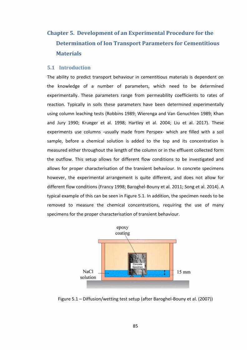
85
Chapter 5. Development of an Experimental Procedure for the
Determination of Ion Transport Parameters for Cementitious
Materials
5.1 Introduction
The ability to predict transport behaviour in cementitious materials is dependent on
the knowledge of a number of parameters, which need to be determined
experimentally. These parameters range from permeability coefficients to rates of
reaction. Typically in soils these parameters have been determined experimentally
using column leaching tests (Robbins 1989; Wierenga and Van Genuchten 1989; Khan
and Jury 1990; Krueger et al. 1998; Hartley et al. 2004; Liu et al. 2017). These
experiments use columns -usually made from Perspex- which are filled with a soil
sample, before a chemical solution is added to the top and its concentration is
measured either throughout the length of the column or in the effluent collected form
the outflow. This setup allows for different flow conditions to be investigated and
allows for proper characterisation of the transient behaviour. In concrete specimens
however, the experimental arrangement is quite different, and does not allow for
different flow conditions (Francy 1998; Baroghel-Bouny et al. 2011; Song et al. 2014). A
typical example of this can be seen in Figure 5.1. In addition, the specimen needs to be
removed to measure the chemical concentrations, requiring the use of many
specimens for the proper characterisation of transient behaviour.
Figure 5.1 – Diffusion/wetting test setup (after Baroghel-Bouny et al. (2007))
86
This chapter presents the development of a methodology to undertake ion transport
experiments in cementitious materials, including the experimental set up and
methodology, the concrete mix design, the experimental results and the difficulties
encountered. The objective of these experiments is to provide a simple means of
obtaining transport parameters for cementitious materials that (i) are quick, (ii) allow
for different flow conditions and (iii) allow for in situ measurements. The results of
these experiments will then be used to validate the numerical model developed in
Chapter 4.
The experimental setup and procedure are detailed in section 5.2 including the
description of the basic premise of the experiments, the design of the tanks and the
detailed description of the experimental procedure.
Section 5.3 details the design of a high porosity concrete, designed to reduce the
amount of time required to carry out the experiments.
The results of an advective-diffusive reactive case concerning Cl- and Na+ are
presented in section 5.4.
The difficulties that were encountered and the steps taken to circumvent them are
presented in section 5.5.
Finally the conclusions on the success of the proposed experiments are made in
section 5.6.
5.2 Experimental Setup and Methodology
The three problems with the current approaches found in the literature that this thesis
aims to address are:
1. The experiments are slow due to the low permeability of concrete, requiring
the use of short specimens.
2. The pressure head cannot be altered, limiting the flow conditions that may be
investigated.
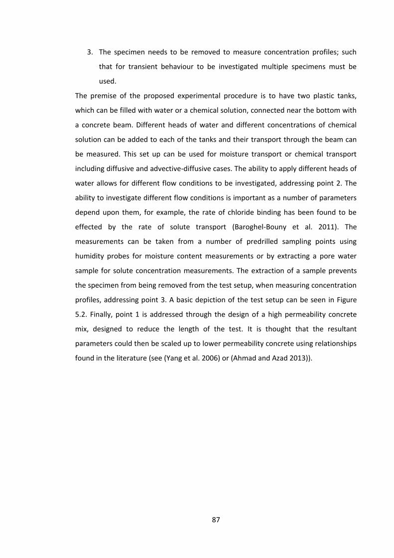
87
3. The specimen needs to be removed to measure concentration profiles; such
that for transient behaviour to be investigated multiple specimens must be
used.
The premise of the proposed experimental procedure is to have two plastic tanks,
which can be filled with water or a chemical solution, connected near the bottom with
a concrete beam. Different heads of water and different concentrations of chemical
solution can be added to each of the tanks and their transport through the beam can
be measured. This set up can be used for moisture transport or chemical transport
including diffusive and advective-diffusive cases. The ability to apply different heads of
water allows for different flow conditions to be investigated, addressing point 2. The
ability to investigate different flow conditions is important as a number of parameters
depend upon them, for example, the rate of chloride binding has been found to be
effected by the rate of solute transport (Baroghel-Bouny et al. 2011). The
measurements can be taken from a number of predrilled sampling points using
humidity probes for moisture content measurements or by extracting a pore water
sample for solute concentration measurements. The extraction of a sample prevents
the specimen from being removed from the test setup, when measuring concentration
profiles, addressing point 3. A basic depiction of the test setup can be seen in Figure
5.2. Finally, point 1 is addressed through the design of a high permeability concrete
mix, designed to reduce the length of the test. It is thought that the resultant
parameters could then be scaled up to lower permeability concrete using relationships
found in the literature (see (Yang et al. 2006) or (Ahmad and Azad 2013)).
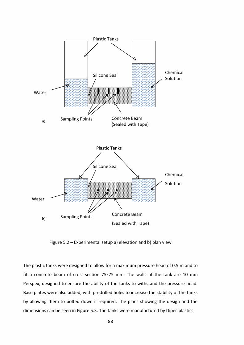
88
Figure 5.2 – Experimental setup a) elevation and b) plan view
The plastic tanks were designed to allow for a maximum pressure head of 0.5 m and to
fit a concrete beam of cross-section 75x75 mm. The walls of the tank are 10 mm
Perspex, designed to ensure the ability of the tanks to withstand the pressure head.
Base plates were also added, with predrilled holes to increase the stability of the tanks
by allowing them to bolted down if required. The plans showing the design and the
dimensions can be seen in Figure 5.3. The tanks were manufactured by Dipec plastics.
Sampling Points
Plastic Tanks
Concrete Beam (Sealed with Tape)
Chemical Solution
Water
Silicone Seal
Water
Chemical
Solution
Silicone Seal
Sampling Points Concrete Beam
(Sealed with Tape)
Plastic Tanks
a)
b)
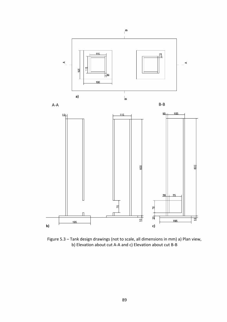
89
Figure 5.3 – Tank design drawings (not to scale, all dimensions in mm) a) Plan view, b) Elevation about cut A-A and c) Elevation about cut B-B
a)
b) c)
A-A B-B
90
5.2.1 Experimental Procedure
5.2.1.1 Beam Preparation
The first step in the experimental procedure is the preparation of the concrete beams,
beginning with the mixing and casting. All concrete mixes were made with a minimum
volume of 10 litres to reduce the effect of moisture loss to the walls of the mixer. To
cast the specimens the moulds were first oiled, to prevent any bonding between the
concrete and the mould walls. Two concrete beams of size 255x75x75 mm and three
concrete cubes of 100x100x100 mm for strength testing were cast each time. Typically,
the strength of the concrete mix used was 15±1 MPa. The strength was measured as a
parameter that could be used to scale the transport properties of the porous concrete
mix to that of an ordinary (lower porosity) concrete (see for example (Al-amoudi et al.
2009)). The moulds were then filled in three layers, with each layer being compacted
using a vibrating table before the next is added. Following a waiting period of 24 hours
the specimens were de-moulded and placed into curing tanks to moist cure in tap
water for 7 days at 19±2 °C.
After 7 days the specimens were taken out of the curing tanks to be prepared for the
experiment. This included the drilling of the holes at the sampling points and the
grinding down of the edge of the sample. This last step was introduced in order to
facilitate the placement of the beams into the plastic tanks, as it was found that the
cross-section of the beams and the cut outs in the plastic tanks were exactly the same
size, making the beams impossible to place. To grind down the edges, an angle grinder
was used, reducing the cross-section at the end of the beams until they fit into the cut
outs of the tanks. Some example photos of a prepared beam can be seen in Figure 5.4
(it should be noted that this beam has been cut in half to reduce its size to
125x75x75 mm, in order to reduce the length of time of the experiment further).
91
Figure 5.4 – Prepared beam (not to scale)
Following this the specimens were placed in an oven at a temperature of 90±2 °C for
24 hours. The main purpose of this was to speed up the hydration reaction, allowing
for shorter curing times, however this may also be used to reduce the moisture
content of the specimen in preparation for test scenarios involving moisture transport.
5.2.1.2 Sealing
The next step was to seal the sides of the concrete beam and place the beam into the
tanks. It was found that Duck ‘Ultimate cloth tape mesh clear’ was the most suitable
for this, which was for two reasons, firstly the cloth tape had a good level of adhesion
to the concrete (when compared to duct tape), and secondly the tape is clear so it
allows a degree of observation (for example in a moisture transport test scenario the
penetration of the wetting front can be seen). Some example photos of the beam
sealed with the cloth tape can be seen in Figure 5.5.
92
Figure 5.5 – Sealed beam (not to scale)
For the placement of the beams into the tanks a layer of silicone was first placed along
the edges of the beam, before pushing each end into the tank cut outs, one by one.
Following this an outer layer of silicone was added around the edge of the cut outs to
seal the connection between the beam and the tanks. Different types of silicone were
tested for their adhesion, with Geocel 'The Works’ being found to give the best results
(in terms of reduced occurrence of leaks) after a number of tests. Some example
photos of the concrete beam in place in the tanks can be seen in Figure 5.6. This setup
was then left for the silicone to cure for 24 hours. If the moisture transport is being
measured it is at this point that humidity probes can be placed into the sampling holes
and linked to a data logger to record the measurements. The moisture transport,
however, was not measured in this study.

93
Figure 5.6 – Silicone seal between beam and tanks
5.2.1.3 Test Setup
Once the silicone was cured the test could be set up, beginning with the addition of
water into the tanks at the desired levels. The next step depended upon the test
scenario being investigated. If the test scenario considered ion transport beginning
with the beam as unsaturated, the chemicals under consideration were added to the
tanks –and stirred into the water to create a solution- as desired immediately. If the
test scenario assumed a saturated beam at the beginning of the test, then this setup
94
was left for one week, to allow the beam to become saturated, before adding the
chemicals. This is considered long enough for full saturation as in wetting tests
cementitious materials have been reported to reach very high saturation after just 48
hours (Baroghel-Bouny et al. 2011). The specimen lengths were smaller (20mm
compared with 125mm) in Baroghel-Bouny et al. (2011), however the porosity of the
concrete used here was much higher, such that time to saturation can be expected to
be lower. In addition to this moisture could be seen on the opposite face after just a
few days. Some example photos of a test setup can be seen in Figure 5.7.
Figure 5.7 – Advective diffusive test setup
The final step was the taking of measurements of the chemical concentrations.
Samples were taken through the extraction of 1 ml of pore fluid from the sampling
95
points, before the hole was resealed with cloth tape. The samples were then analysed
for their chemical content. For salts this analysis was carried out using a Mettler
Toledo SevenMulti, which was used to measure the total dissolved solids (TDS) content
of the solution. The Toledo SevenMulti was calibrated against a control solution and
has an accuracy of ±0.5 %. Due to the fact that some cementitious ions are present in
the pore water phase, a control test was needed in order to determine what
proportion of the measured TDS content represented the additional chemicals. The
control case setup was the same as the test case, but this time no additional chemicals
were added. The difference between the TDS of the test case and the TDS of the
control gives the concentration of the chemicals added. For more complex chemical
systems, the sample taken could be analysed using alternative methods such as
spectroscopy; however this was not undertaken in this study.
The general procedure can be summarised into the following 10 steps:
1. Cast the concrete specimens.
2. Place the specimens in a curing tank for 7 days.
3. Cut the beams to size, prepare the edges and drill holes at the sampling points.
4. Place the specimens in oven at 90 °Cfor 24 hours.
5. Seal the beam with cloth tape before sealing into place in the tank cut outs
with silicone.
6. Leave the silicone to cure for 24 hours.
7. Fill the tanks with desired levels of water.
8. Add the chemicals after 1 week for an initially saturated case or immediately
for an initially unsaturated case.
9. Take samples from sampling points at desired times using a syringe, and reseal.
10. Measure the chemical concentrations using a conductivity measure or other
method and compare this value with a control case.
5.3 Concrete Mix Design
The aim of the concrete mix design was to produce a concrete with a high porosity
such that the time taken for each experiment was reduced but a low enough porosity
that the concrete is still similar to an ordinary concrete mix as opposed to a pervious
96
concrete (which are no fines concretes developed for use as pavements, designed to
allow the quick transfer of rainwater into the underlying soil (Yang and Jiang 2003)). It
was thought that if the concrete mix is designed in this way then it will be possible to
compare the results of the experiments with ordinary concrete mixes or to scale up
the resultant parameters to higher strength/lower porosity concretes by using
relationships found in the literature (see (Yang et al. 2006) or (Ahmad and Azad 2013)).
To achieve this balance in porosity between that of a pervious and an ordinary
concrete, a very high w/c ratio of 0.9 was used, which has been found to increase the
porosity (Kim et al. 2014), along with a low percentage of fine aggregate. Three
different concrete mixes were tested, denoted as L, M and H, with fine aggregate
contents of 10 %, 15 % and 20 % respectively. The full details of the concrete mixes can
be seen in Table 5.1. The materials used were Portland-fly ash cement (CEM II/B-V
32,5R), 4-10 mm crushed limestone and 0-4 mm sea dredged sand. The grading curves
for the aggregates, determined according to BS EN 12620:2013, are shown in Figure
5.8.
Table 5.1 – Mix parameters
Parameter Mix
L M H
Fine Aggregate %agea (%) 10 15 20
W/C Ratio 0.9 0.9 0.9
Water Content (kg) 2.25 2.25 2.25
Cement Content (kg) 2.5 2.5 2.5
Coarse Aggregate Content (kg) 16.61 15.68 14.76
Fine Aggregate Content (kg) 1.85 2.77 3.69 aPercentage of total aggregate content
97
Figure 5.8 – Grading curves for a) Coarse aggregate and b) Fine aggregate
The main problem with using such a low fine aggregate content was that when the
specimen was compacted, the fine aggregate sank to the bottom of the specimen,
producing a beam with the bottom half containing all of the fine aggregate and the top
half containing only coarse aggregate. Such aggregation of samples is shown in Figure
5.9 for the resultant specimens of the L mix.
The specimen photos of the M mix can be seen in Figure 5.10. It can be seen that the
sinking of the fine aggregate was still a problem for this mix, albeit to a lesser extent.
Finally the specimen photos of the H mix can be seen in Figure 5.11. Here the sinking
of fine aggregate is significantly less pronounced and can only be seen in one of the
concrete cubes. These photos show that this mix is capable of producing a suitable
concrete, and so it was this mix that was used in the experiments.
0
10
20
30
40
50
60
70
80
90
100
0.006 0.6 60
Pe
rce
nta
ge p
assi
ng
(%)
Sieve size (mm) a)
0
10
20
30
40
50
60
70
80
90
100
0.006 0.6 60
Pe
rce
nta
ge p
assi
ng
(%)
Sieve size (mm) b)
98
Figure 5.9 – Mix L specimens (not to scale)
99
Figure 5.10 – Mix M specimens (not to scale)
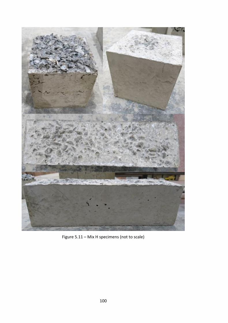
100
Figure 5.11 – Mix H specimens (not to scale)
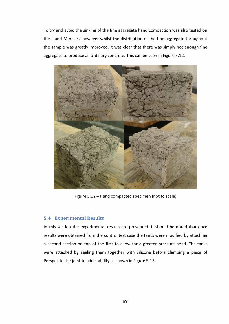
101
To try and avoid the sinking of the fine aggregate hand compaction was also tested on
the L and M mixes; however whilst the distribution of the fine aggregate throughout
the sample was greatly improved, it was clear that there was simply not enough fine
aggregate to produce an ordinary concrete. This can be seen in Figure 5.12.
Figure 5.12 – Hand compacted specimen (not to scale)
5.4 Experimental Results
In this section the experimental results are presented. It should be noted that once
results were obtained from the control test case the tanks were modified by attaching
a second section on top of the first to allow for a greater pressure head. The tanks
were attached by sealing them together with silicone before clamping a piece of
Perspex to the joint to add stability as shown in Figure 5.13.
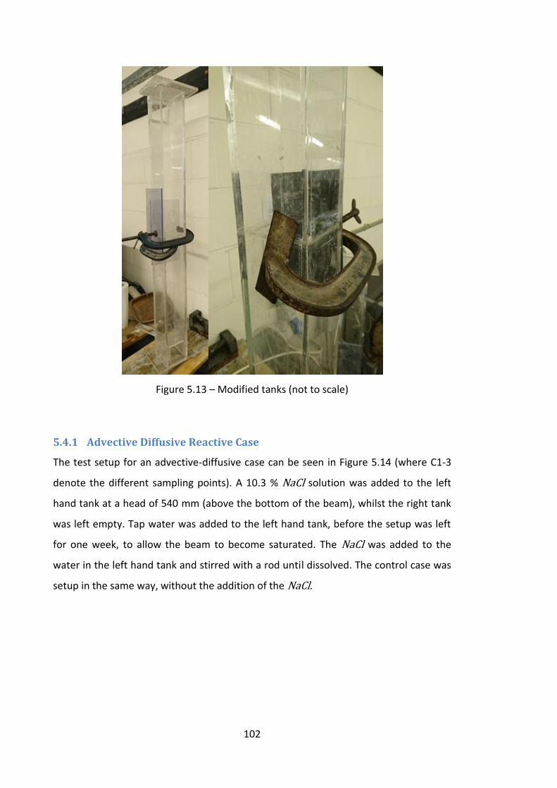
102
Figure 5.13 – Modified tanks (not to scale)
5.4.1 Advective Diffusive Reactive Case
The test setup for an advective-diffusive case can be seen in Figure 5.14 (where C1-3
denote the different sampling points). A 10.3 % NaCl solution was added to the left
hand tank at a head of 540 mm (above the bottom of the beam), whilst the right tank
was left empty. Tap water was added to the left hand tank, before the setup was left
for one week, to allow the beam to become saturated. The NaCl was added to the
water in the left hand tank and stirred with a rod until dissolved. The control case was
setup in the same way, without the addition of the NaCl.
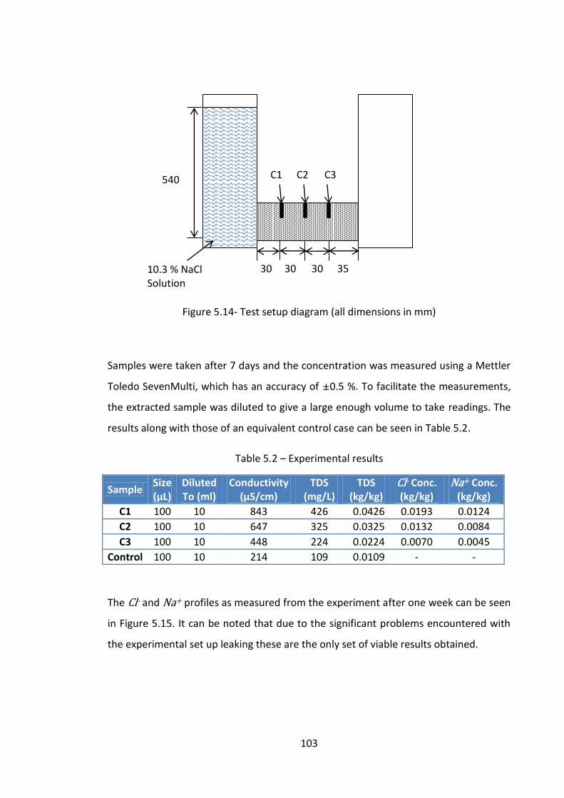
103
Figure 5.14- Test setup diagram (all dimensions in mm)
Samples were taken after 7 days and the concentration was measured using a Mettler
Toledo SevenMulti, which has an accuracy of ±0.5 %. To facilitate the measurements,
the extracted sample was diluted to give a large enough volume to take readings. The
results along with those of an equivalent control case can be seen in Table 5.2.
Table 5.2 – Experimental results
Sample Size (μL)
Diluted To (ml)
Conductivity (μS/cm)
TDS (mg/L)
TDS (kg/kg)
Cl- Conc. (kg/kg)
Na+ Conc. (kg/kg)
C1 100 10 843 426 0.0426 0.0193 0.0124
C2 100 10 647 325 0.0325 0.0132 0.0084
C3 100 10 448 224 0.0224 0.0070 0.0045
Control 100 10 214 109 0.0109 - -
The Cl- and Na+ profiles as measured from the experiment after one week can be seen
in Figure 5.15. It can be noted that due to the significant problems encountered with
the experimental set up leaking these are the only set of viable results obtained.
10.3 % NaCl Solution
30 30 30 35
540 C1 C2 C3
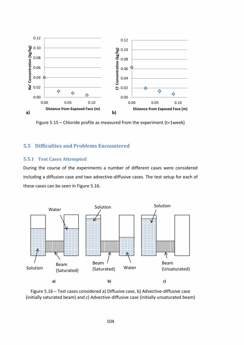
104
Figure 5.15 – Chloride profile as measured from the experiment (t=1week)
5.5 Difficulties and Problems Encountered
5.5.1 Test Cases Attempted
During the course of the experiments a number of different cases were considered
including a diffusion case and two advective-diffusive cases. The test setup for each of
these cases can be seen in Figure 5.16.
Figure 5.16 – Test cases considered a) Diffusive case, b) Advective-diffusive case (initially saturated beam) and c) Advective-diffusive case (initially unsaturated beam)
0.00
0.02
0.04
0.06
0.08
0.10
0.12
0.00 0.05 0.10
Na+
Co
nce
ntr
atio
n (
kg/k
g)
Distance from Exposed Face (m) a)
0.00
0.02
0.04
0.06
0.08
0.10
0.12
0.00 0.05 0.10
Cl- C
on
cen
trat
ion
(kg
/kg)
Distance from Exposed Face (m) b)
Solution
Water Solution
Water
Solution
Beam (Saturated)
Beam (Saturated)
Beam (Unsaturated)
a) b) c)
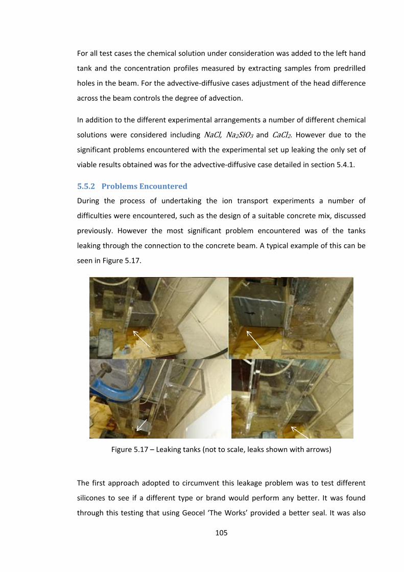
105
For all test cases the chemical solution under consideration was added to the left hand
tank and the concentration profiles measured by extracting samples from predrilled
holes in the beam. For the advective-diffusive cases adjustment of the head difference
across the beam controls the degree of advection.
In addition to the different experimental arrangements a number of different chemical
solutions were considered including NaCl, Na2SiO3 and CaCl2. However due to the
significant problems encountered with the experimental set up leaking the only set of
viable results obtained was for the advective-diffusive case detailed in section 5.4.1.
5.5.2 Problems Encountered
During the process of undertaking the ion transport experiments a number of
difficulties were encountered, such as the design of a suitable concrete mix, discussed
previously. However the most significant problem encountered was of the tanks
leaking through the connection to the concrete beam. A typical example of this can be
seen in Figure 5.17.
Figure 5.17 – Leaking tanks (not to scale, leaks shown with arrows)
The first approach adopted to circumvent this leakage problem was to test different
silicones to see if a different type or brand would perform any better. It was found
through this testing that using Geocel ‘The Works’ provided a better seal. It was also
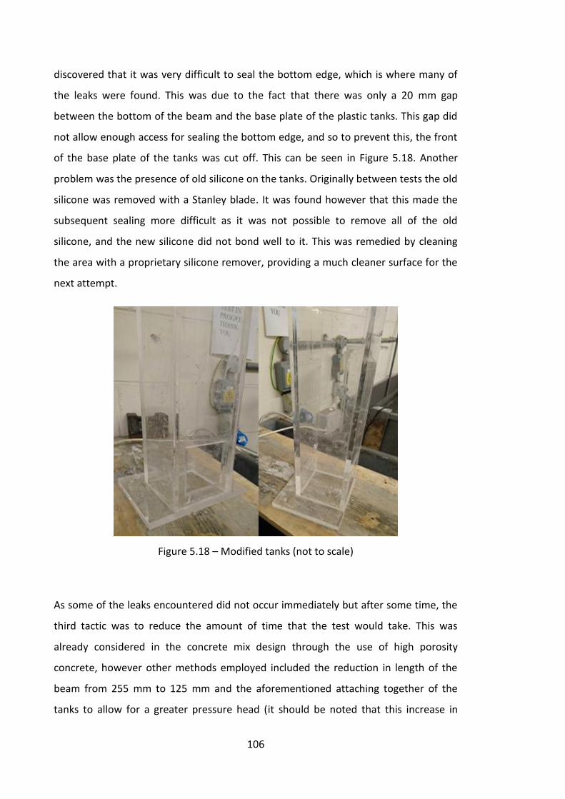
106
discovered that it was very difficult to seal the bottom edge, which is where many of
the leaks were found. This was due to the fact that there was only a 20 mm gap
between the bottom of the beam and the base plate of the plastic tanks. This gap did
not allow enough access for sealing the bottom edge, and so to prevent this, the front
of the base plate of the tanks was cut off. This can be seen in Figure 5.18. Another
problem was the presence of old silicone on the tanks. Originally between tests the old
silicone was removed with a Stanley blade. It was found however that this made the
subsequent sealing more difficult as it was not possible to remove all of the old
silicone, and the new silicone did not bond well to it. This was remedied by cleaning
the area with a proprietary silicone remover, providing a much cleaner surface for the
next attempt.
Figure 5.18 – Modified tanks (not to scale)
As some of the leaks encountered did not occur immediately but after some time, the
third tactic was to reduce the amount of time that the test would take. This was
already considered in the concrete mix design through the use of high porosity
concrete, however other methods employed included the reduction in length of the
beam from 255 mm to 125 mm and the aforementioned attaching together of the
tanks to allow for a greater pressure head (it should be noted that this increase in
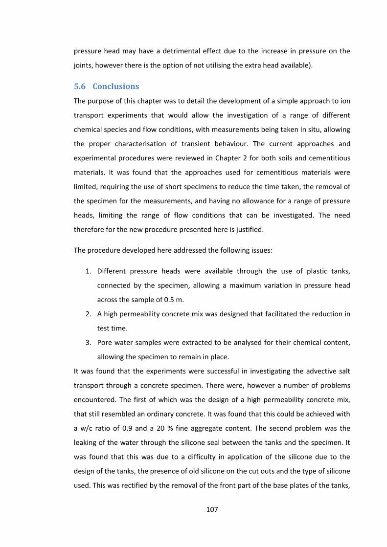
107
pressure head may have a detrimental effect due to the increase in pressure on the
joints, however there is the option of not utilising the extra head available).
5.6 Conclusions
The purpose of this chapter was to detail the development of a simple approach to ion
transport experiments that would allow the investigation of a range of different
chemical species and flow conditions, with measurements being taken in situ, allowing
the proper characterisation of transient behaviour. The current approaches and
experimental procedures were reviewed in Chapter 2 for both soils and cementitious
materials. It was found that the approaches used for cementitious materials were
limited, requiring the use of short specimens to reduce the time taken, the removal of
the specimen for the measurements, and having no allowance for a range of pressure
heads, limiting the range of flow conditions that can be investigated. The need
therefore for the new procedure presented here is justified.
The procedure developed here addressed the following issues:
1. Different pressure heads were available through the use of plastic tanks,
connected by the specimen, allowing a maximum variation in pressure head
across the sample of 0.5 m.
2. A high permeability concrete mix was designed that facilitated the reduction in
test time.
3. Pore water samples were extracted to be analysed for their chemical content,
allowing the specimen to remain in place.
It was found that the experiments were successful in investigating the advective salt
transport through a concrete specimen. There were, however a number of problems
encountered. The first of which was the design of a high permeability concrete mix,
that still resembled an ordinary concrete. It was found that this could be achieved with
a w/c ratio of 0.9 and a 20 % fine aggregate content. The second problem was the
leaking of the water through the silicone seal between the tanks and the specimen. It
was found that this was due to a difficulty in application of the silicone due to the
design of the tanks, the presence of old silicone on the cut outs and the type of silicone
used. This was rectified by the removal of the front part of the base plates of the tanks,

108
the use of a silicone remover between tests and the testing of different silicones until a
suitable one was found.
It is recognised that, due to the problems encountered, a limited number of results
were produced, however it has been shown that once these problems were addressed
the experimental procedure was effective in providing a simple means of investigating
ion transport through a concrete specimen under different flow conditions.
109
Chapter 6. Verification and Validation of the Coupled Model
6.1 Introduction
This chapter details the verification and validation of the full transport model through
a series of numerical simulations of example problems found in the literature. This
chapter is split into two main parts; the first part concerns the verification of the
model, to this end the model is compared to a number of numerical simulations
reported in the literature concerning the reactive transport of chemical species
through concrete and mortar specimens. The second part concerns the validation of
the model, which will be carried out by considering the experimental results of the
drying of three different mixes of concrete specimens found in Kim and Lee (1999), and
the experimental results obtained from the ion transport experiments, details of which
were presented in Chapter 5.
Section 6.2 details the verification of the model. This section begins with examples
from Koniorczyk (2010) and Koniorczyk and Gawin (2012), concerning the transport
and precipitation of salt in building materials. Following these, examples from
Baroghel-Bouny et al. (2011) and Song et el. (2014) concerning multiple ionic transport
in cementitious specimens are then simulated.
The validation of the moisture flow and chemical transport can be found in section 6.3,
where simulations were carried out based on the drying experiments reported by Kim
and Lee (1999) and the results of the ion transport experiments reported in chapter 5.
Finally in section 6.4 the conclusions drawn on the ability of the model to accurately
simulate the various transport problems are presented.
6.2 Verification of the Coupled Model
6.2.1 Introduction
In this section the verification of the full reactive transport model will be presented
through a series of examples concerning reactive chemical transport in cementitious
materials. The first two examples are taken from Koniorczyk (2010) and Koniorczyk and
Gawin (2012), which concern the drying of building materials initially saturated with a
salt solution. In both examples the precipitation of the salt was included with an
110
assumption of non-equilibrium conditions, with the difference being that in the first
example the rate of reaction was calculated as a function of the concentration and in
the second it was calculated instead as a function of the solution supersaturation ratio.
The final two examples were presented by Baroghel-Bouny et al. (2011) and Song et al.
(2014) respectively. They concern the multi-ionic diffusion of chemical species from a
source solution into a cementitious material. The chemical reactions found in both
examples are modelled with an assumption of non-equilibrium conditions using a
Freundlich type isotherm. In addition to this both examples also included a charge
neutrality condition through the implementation of the Nernst Planck and Poisson
equations, with the difference being that Baroghel-Bouny et al. (2011) solved for the
electrical potential as a primary variable, whereas Song et al. (2014) substituted the
condition of zero current directly into the diffusive flux equation, eliminating the
electrical potential as a variable.
For all examples the mesh and time step sizes were chosen based on the results of a
mesh convergence study.
6.2.2 Example – Koniorczyk (2010)
In 2010 Koniorczyk (2010) developed a model to simulate the transport and
crystallisation of salt in porous building materials. The simulations undertaken included
the drying of a mortar sample containing NaCl and the cool-warming of a cement
mortar containing Na2SO4. For the drying simulation, both the equilibrium and non-
equilibrium approach to the salt precipitation were considered, with the equilibrium
approach testing Freundlich, linear and Langmuir isotherms and the non-equilibrium
approach testing a kinetic Freundlich isotherm. The results considered here were of
the drying of the mortar sample containing NaCl with non-equilibrium salt
precipitation. The rate of reaction is of the general from of eq. (3.39) and is given as:
( ) (6.1)
where is a rate parameter, λ is the order of the reaction, A’ is a supersaturation
parameter given here as 1 and cmax is the solubility of NaCl.
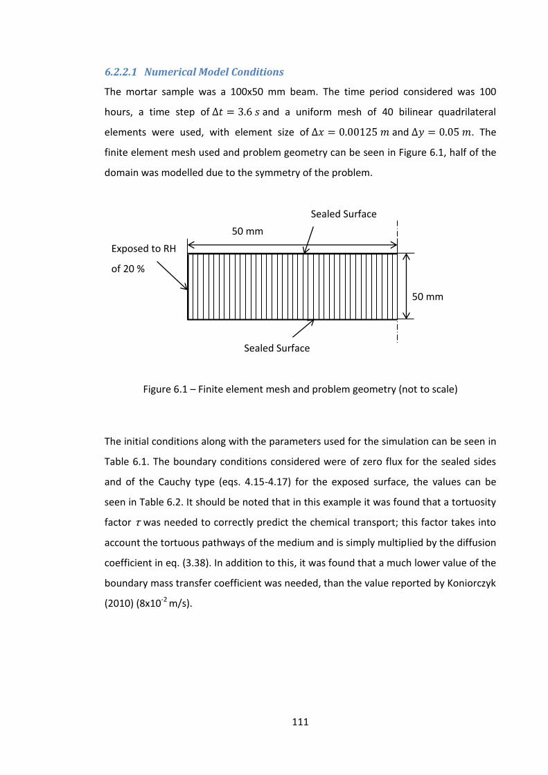
111
6.2.2.1 Numerical Model Conditions
The mortar sample was a 100x50 mm beam. The time period considered was 100
hours, a time step of and a uniform mesh of 40 bilinear quadrilateral
elements were used, with element size of and . The
finite element mesh used and problem geometry can be seen in Figure 6.1, half of the
domain was modelled due to the symmetry of the problem.
Figure 6.1 – Finite element mesh and problem geometry (not to scale)
The initial conditions along with the parameters used for the simulation can be seen in
Table 6.1. The boundary conditions considered were of zero flux for the sealed sides
and of the Cauchy type (eqs. 4.15-4.17) for the exposed surface, the values can be
seen in Table 6.2. It should be noted that in this example it was found that a tortuosity
factor τ was needed to correctly predict the chemical transport; this factor takes into
account the tortuous pathways of the medium and is simply multiplied by the diffusion
coefficient in eq. (3.38). In addition to this, it was found that a much lower value of the
boundary mass transfer coefficient was needed, than the value reported by Koniorczyk
(2010) (8x10⁻² m/s).
50 mm
50 mm
Exposed to RH
of 20 %
Sealed Surface
Sealed Surface
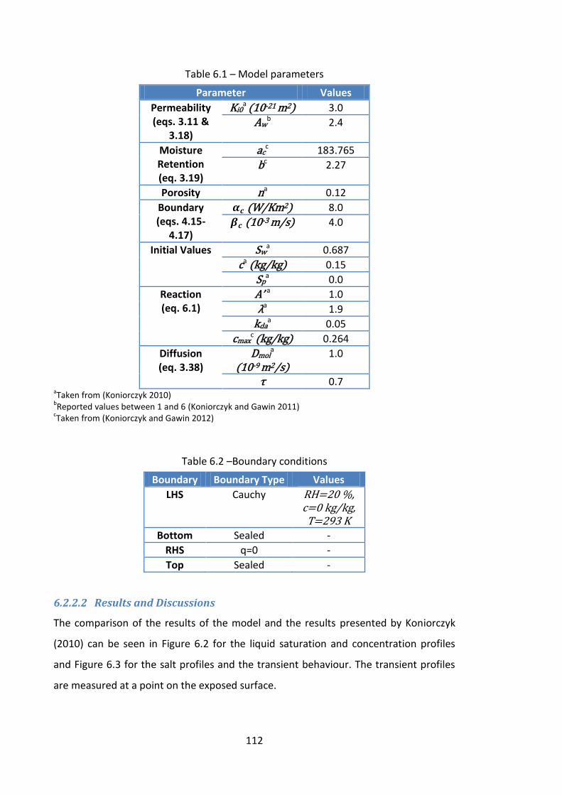
112
Table 6.1 – Model parameters
Parameter Values
Permeability (eqs. 3.11 &
3.18)
Ki0a
(10-21 m2) 3.0
Awb 2.4
Moisture Retention (eq. 3.19)
acc 183.765
bc 2.27
Porosity na 0.12
Boundary (eqs. 4.15-
4.17)
(W/Km2) 8.0
(10-3 m/s) 4.0
Initial Values Swa 0.687
ca (kg/kg) 0.15
Spa 0.0
Reaction (eq. 6.1)
A’ a 1.0
λa 1.9
kdaa 0.05
cmaxc (kg/kg) 0.264
Diffusion (eq. 3.38)
Dmola
(10-9 m2/s) 1.0
τ 0.7 aTaken from (Koniorczyk 2010)
bReported values between 1 and 6 (Koniorczyk and Gawin 2011)
cTaken from (Koniorczyk and Gawin 2012)
Table 6.2 –Boundary conditions
Boundary Boundary Type Values
LHS Cauchy RH=20 %, c=0 kg/kg, T=293 K
Bottom Sealed -
RHS q=0 -
Top Sealed -
6.2.2.2 Results and Discussions
The comparison of the results of the model and the results presented by Koniorczyk
(2010) can be seen in Figure 6.2 for the liquid saturation and concentration profiles
and Figure 6.3 for the salt profiles and the transient behaviour. The transient profiles
are measured at a point on the exposed surface.
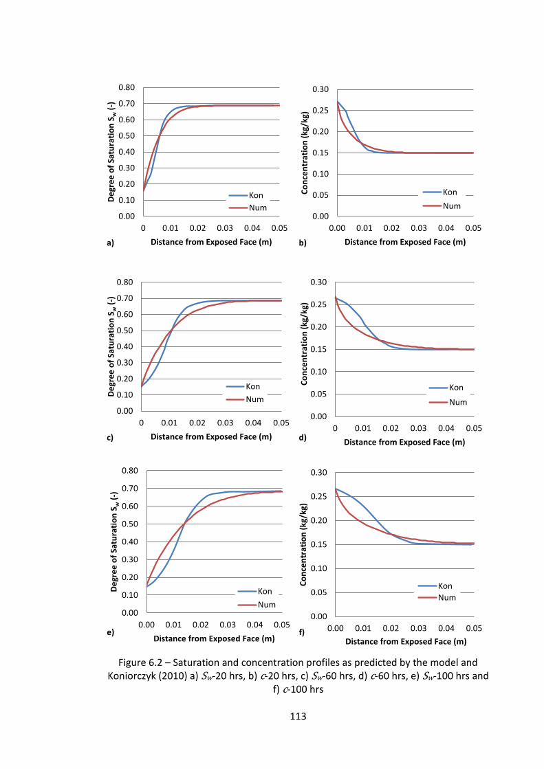
113
Figure 6.2 – Saturation and concentration profiles as predicted by the model and Koniorczyk (2010) a) Sw-20 hrs, b) c-20 hrs, c) Sw-60 hrs, d) c-60 hrs, e) Sw-100 hrs and
f) c-100 hrs
0.00
0.10
0.20
0.30
0.40
0.50
0.60
0.70
0.80
0 0.01 0.02 0.03 0.04 0.05
De
gre
e o
f Sa
tura
tio
n S
w (
-)
Distance from Exposed Face (m) a)
Kon
Num0.00
0.05
0.10
0.15
0.20
0.25
0.30
0.00 0.01 0.02 0.03 0.04 0.05
Co
nce
ntr
atio
n (
kg/k
g)
Distance from Exposed Face (m) b)
Kon
Num
0.00
0.10
0.20
0.30
0.40
0.50
0.60
0.70
0.80
0 0.01 0.02 0.03 0.04 0.05
De
gre
e o
f Sa
tura
tio
n S
w (
-)
Distance from Exposed Face (m) c)
Kon
Num
0.00
0.05
0.10
0.15
0.20
0.25
0.30
0 0.01 0.02 0.03 0.04 0.05
Co
nce
ntr
atio
n (
kg/k
g)
Distance from Exposed Face (m) d)
Kon
Num
0.00
0.10
0.20
0.30
0.40
0.50
0.60
0.70
0.80
0.00 0.01 0.02 0.03 0.04 0.05
De
gre
e o
f Sa
tura
tio
n S
w (
-)
Distance from Exposed Face (m) e)
Kon
Num
0.00
0.05
0.10
0.15
0.20
0.25
0.30
0.00 0.01 0.02 0.03 0.04 0.05
Co
nce
ntr
atio
n (
kg/k
g)
Distance from Exposed Face (m) f)
Kon
Num
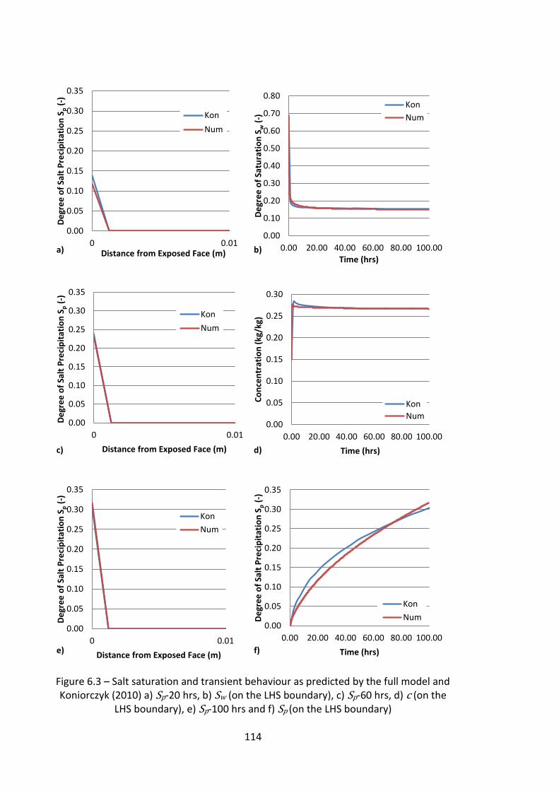
114
Figure 6.3 – Salt saturation and transient behaviour as predicted by the full model and Koniorczyk (2010) a) Sp-20 hrs, b) Sw (on the LHS boundary), c) Sp-60 hrs, d) c (on the
LHS boundary), e) Sp-100 hrs and f) Sp (on the LHS boundary)
0.00
0.05
0.10
0.15
0.20
0.25
0.30
0.35
0 0.01
De
gre
e o
f Sa
lt P
reci
pit
atio
n S
p (
-)
Distance from Exposed Face (m) a)
Kon
Num
0.00
0.10
0.20
0.30
0.40
0.50
0.60
0.70
0.80
0.00 20.00 40.00 60.00 80.00 100.00D
egr
ee
of
Satu
rati
on
Sw
(-)
Time (hrs)
b)
Kon
Num
0.00
0.05
0.10
0.15
0.20
0.25
0.30
0.35
0 0.01
De
gre
e o
f Sa
lt P
reci
pit
atio
n S
p (
-)
Distance from Exposed Face (m) c)
Kon
Num
0.00
0.05
0.10
0.15
0.20
0.25
0.30
0.00 20.00 40.00 60.00 80.00 100.00
Co
nce
ntr
atio
n (
kg/k
g)
Time (hrs) d)
Kon
Num
0.00
0.05
0.10
0.15
0.20
0.25
0.30
0.35
0 0.01
De
gre
e o
f Sa
lt P
reci
pit
atio
n S
p (
-)
Distance from Exposed Face (m) e)
Kon
Num
0.00
0.05
0.10
0.15
0.20
0.25
0.30
0.35
0.00 20.00 40.00 60.00 80.00 100.00
De
gre
e o
f Sa
lt P
reci
pit
atio
n S
p (
-)
Time (hrs) f)
Kon
Num
115
It can be seen from the profiles that the model is generally in good agreement with the
results found in (Koniorczyk 2010). The degree of salt saturation shows good
agreement for the 20, 60 and 100 hour profiles and the transient profiles of each of
the variables are well matched. The profiles that are not as well matched are those of
the liquid saturation and dissolved chemical concentration. The dissolved chemical
concentration however depends on the degree of saturation as it is measured as mass
per mass of liquid, and it can be seen that where the chemical concentration is over
predicted the degree of saturation is under predicted and vice versa, therefore it is
likely that the difference in concentration profiles is as a result of the difference in the
liquid saturation profiles. The moisture models however are different and it is
uncertain what values of parameters (such as the coefficients of both the moisture
retention curve (eq. 3.19) and the permeability-saturation relation which were not
reported by Koniorczyk (2010)) were used for the moisture flow. This difference may
have arisen due to the fact that Koniorczyk (2010) has taken into account the effect of
the salt on the moisture retention curve (Koniorczyk and Wojciechowski 2009), which
can have a significant effect at high salt concentrations (Koniorczyk and Wojciechowski
2009) and which has not been accounted for in this thesis. The purpose of this example
was to verify the chemical transport and precipitation, as the moisture transport will
be validated later in section 6.3, meaning that it is justified to fit the model moisture
results close to those of Koniorczyk (2010).
6.2.3 Example – Koniorczyk & Gawin (2012)
In 2012 Koniorczyk and Gawin (2012) developed the previous model (Koniorczyk 2010)
further and considered the salt crystallisation pressure that is exerted on the solid
skeleton. The salt crystallisation was considered with an assumption of non-
equilibrium conditions using a Freundlich type isotherm as before, the difference being
that in this approach the rate of precipitation was driven by the solution
supersaturation ratio instead of the chemical concentration. The solution
supersaturation ratio was calculated from the ion activity, which was calculated using
an ion interaction model. To this end the Pitzer equations were preferred as a result of
their higher range of validity than the Debye-Hückel or Davies models, which is
important for the concentrations present in salt crystallisation problems. The examples
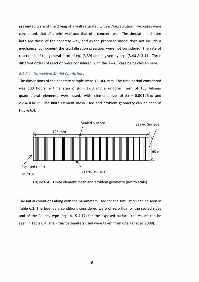
116
presented were of the drying of a wall saturated with a NaCl solution. Two cases were
considered, that of a brick wall and that of a concrete wall. The simulations chosen
here are those of the concrete wall, and as the proposed model does not include a
mechanical component the crystallisation pressures were not considered. The rate of
reaction is of the general form of eq. (3.39) and is given by eqs. (3.40 & 3.41). Three
different orders of reaction were considered, with the λ case being chosen here.
6.2.3.1 Numerical Model Conditions
The dimensions of the concrete sample were 125x60 mm. The time period considered
was 100 hours, a time step of and a uniform mesh of 100 bilinear
quadrilateral elements were used, with element size of and
. The finite element mesh used and problem geometry can be seen in
Figure 6.4.
Figure 6.4 – Finite element mesh and problem geometry (not to scale)
The initial conditions along with the parameters used for the simulation can be seen in
Table 6.3. The boundary conditions considered were of zero flux for the sealed sides
and of the Cauchy type (eqs. 4.15-4.17) for the exposed surface, the values can be
seen in Table 6.4. The Pitzer parameters used were taken from (Steiger et al. 2008).
60 mm
Sealed Surface
125 mm
Sealed Surface Sealed Surface
Exposed to RH
of 20 %
117
Table 6.3 –Model parameters
Parameter Values
Permeability (eqs. 3.11 &
3.18)
Ki0a (10-21 m2) 3.0
Awb 1.0
Moisture Retention (eq. 3.19)
aca 183.834
ba 2.27
Porosity na 0.131
Boundary (eqs. 4.15-
4.17)
(W/Km2) 8.0
(10-3 m/s) 2.6
Initial Values Swa 1.0
ca (kg/kg) 0.1
Spa 0.0
Reaction (eqs. 3.40 &
3.41)
A’ 1.4
λa 4.5
kdaa 1.0
A’2 1.3
Diffusion (eq. 3.38)
Dmolc
(10-9 m2/s) 1.0
τ 0.45 aTaken from (Koniorczyk and Gawin 2012)
bReported values between 1 and 6 (Koniorczyk and Gawin 2011)
cTaken from (Koniorczyk 2010)
Table 6.4 – Boundary conditions
Boundary Boundary Type Values
LHS Cauchy RH=60 %, c=0 kg/kg, T=293 K
Bottom Sealed -
RHS Sealed -
Top Sealed -
It should be noted that A’ found in eq. (3.40) is the primary crystallisation coefficient,
which is the supersaturation ratio needed for crystallisation to begin and A’2 is the
secondary crystallisation coefficient. It was unclear which values of A’ and A’2 were
used by Koniorczyk and Gawin (2012) and so values of 1.4 and 1.3 were chosen here
after an initial calibration exercise. The calibration exercise involved changing the
118
values of the parameters on a trial and error (beginning with the moisture parameters)
basis until the resultant profiles were in good agreement with those of Koniorczyk and
Gawin (2012). These values do not lie within the reported ranges quoted by Koniorczyk
and Gawin (2012) however it should be noted that the solubility also depends on the
pore size, needing a higher salt concentration to begin precipitation in smaller pores,
which is not taken into account in this study. The influence of pore size on the
solubility can be seen in Figure 6.5 for three different crystal shapes (reproduced from
Koniorczyk and Gawin (2012), a and ainf are the activities of a solution saturated with
small and large crystals respectively and r is the pore radius). As with the previous
example, it was found in this study that a tortuosity factor was needed to correctly
predict the chemical transport, and the boundary mass transfer coefficient needed
was lower than the value reported by Koniorczyk and Gawin (2012) (8x10⁻³ m/s).
Figure 6.5 – Influence of pore size on salt solubility (after Koniorczyk and Gawin (2012))
6.2.3.2 Results and Discussions
The comparison of the results of the model and the results of Koniorczyk and Gawin
(2012) can be seen in Figure 6.6 for the liquid saturation and supersaturation profiles
and Figure 6.7 for the salt profiles and the transient behaviour. The transient profiles
are measured at a point on the exposed surface.
119
Figure 6.6 – Saturation and solution supersaturation profiles as predicted by the full model and Koniorczyk and Gawin (2012) a) Sw-20 hrs, b) S-20 hrs, c) Sw-60 hrs,
d) S-60 hrs, e) Sw-100 hrs and f) S-100 hrs
0.00
0.10
0.20
0.30
0.40
0.50
0.60
0.70
0.80
0.90
1.00
0.00 0.05 0.10
De
gre
e o
f Sa
tura
tio
n S
w (
-)
Distance from Exposed Face (m) a)
Kon
Num0.00
0.20
0.40
0.60
0.80
1.00
1.20
1.40
1.60
0.00 0.05 0.10
Sup
ers
atu
rati
on
rat
io S
(-)
Distance from Exposed Face (m) b)
Kon
Num
0.00
0.10
0.20
0.30
0.40
0.50
0.60
0.70
0.80
0.90
1.00
0.00 0.05 0.10
De
gre
e o
f Sa
tura
tio
n S
w (
-)
Distance from Exposed Face (m) c)
Kon
Num0.00
0.20
0.40
0.60
0.80
1.00
1.20
1.40
1.60
0.00 0.05 0.10
Sup
ers
atu
rati
on
rat
io S
(-)
Distance from Exposed Face (m) d)
Kon
Num
0.00
0.10
0.20
0.30
0.40
0.50
0.60
0.70
0.80
0.90
1.00
0.00 0.05 0.10
De
gre
e o
f Sa
tura
tio
n S
w (
-)
Distance from Exposed Face (m) e)
Kon
Num0.00
0.20
0.40
0.60
0.80
1.00
1.20
1.40
1.60
0.00 0.05 0.10
Sup
ers
atu
rati
on
rat
io S
(-)
Distance from Exposed Face (m) f)
Kon
Num
120
Figure 6.7 – Salt saturation and transient behaviour as predicted by full model and Koniorczyk and Gawin (2012) a) Sp-20 hrs, b) Sw (on the LHS boundary), c) Sp-60 hrs,
d) S (on the LHS boundary), e) Sp-100 hrs and f) Sp (on the LHS boundary)
0.00
0.10
0.20
0.30
0.40
0.50
0.60
0.70
0.80
0.10 0.11 0.12
De
gre
e o
f Sa
lt P
reci
pit
atio
n S
p (
-)
Distance from Exposed Face (m) a)
Kon
Num
0.00
0.10
0.20
0.30
0.40
0.50
0.60
0.70
0.80
0.90
1.00
0.00 20.00 40.00 60.00 80.00 100.00
De
gre
e o
f Sa
tura
tio
n S
w (
-)
Time (hrs) b)
NumNo Kon Results
0.00
0.10
0.20
0.30
0.40
0.50
0.60
0.70
0.80
0.10 0.11 0.12
De
gre
e o
f Sa
lt P
reci
pit
atio
n S
p (
-)
Distance from Exposed Face (m) c)
Kon
Num
0.00
0.20
0.40
0.60
0.80
1.00
1.20
1.40
1.60
0.00 20.00 40.00 60.00 80.00 100.00
Sup
ers
atu
rati
on
rat
io S
(-)
Time (hrs) d)
KonNum
0.00
0.10
0.20
0.30
0.40
0.50
0.60
0.70
0.80
0.10 0.11 0.12
De
gre
e o
f Sa
lt P
reci
pit
atio
n S
p (
-)
Distance from Exposed Face (m) e)
Kon
Num
0.00
0.10
0.20
0.30
0.40
0.50
0.60
0.70
0.80
0.00 20.00 40.00 60.00 80.00 100.00
De
gre
e o
f Sa
lt P
reci
pit
atio
n S
p (
-)
Time (hrs) f)
Kon
Num
121
It can be seen from the profiles presented in Figures 6.6 and 6.7 that the model is in
good agreement with the simulations of Koniorczyk and Gawin (2012). The
precipitated salt profiles are the best match, with the liquid saturation being slightly
over predicted, as is the supersaturation ratio. The transient behaviour the degree of
salt precipitation is closely matched until around 70 hours where the model begins to
over predict the amount. The solution supersaturation ratio was in the same range of
values but the behaviour was slightly different, instead of increasing to a maximum at
around 9 hours and then gradually decreasing, the model predicts it increasing to a
maximum at around 6 hours, followed by a sharp decrease and then a relatively
constant value therein. This behaviour arises due to the fact that following the initial
salt precipitation the rate of increase of concentration due to the decrease in moisture
content is almost equal to the rate of decrease of concentration due to the salt
precipitation.
6.2.4 Example – Baroghel-Bouny et al. (2011)
In 2011 Baroghel-Bouny et al. (2011) presented a model for the simulation of multi-
ionic transport in cementitious materials. The model included both the consideration
of the chloride binding and formation of Friedel’s salt. The formation of Friedel’s salt
was assumed to be instantaneous, whereas the chloride binding was investigated with
assumptions of both equilibrium and non-equilibrium conditions. It was found that the
non-equilibrium assumption gave a more accurate prediction of the total chloride
content profiles (Tcc) measured in diffusion experiments, with the modelling under
the equilibrium assumption greatly over predicting the Tcc near the surface and
greatly under predicting the chloride penetration depth. It was also assumed that as
the chloride ions bound to the cement matrix, hydroxide ions were simultaneously
released to maintain the charge neutrality of the solution. The rate of reaction can be
described by eq. (3.39), and the formation of Friedel’s salt is given as:
(6.2)
where is a factor derived from stoichiometric considerations and is the
equivalent content of the residual aluminates of the material.
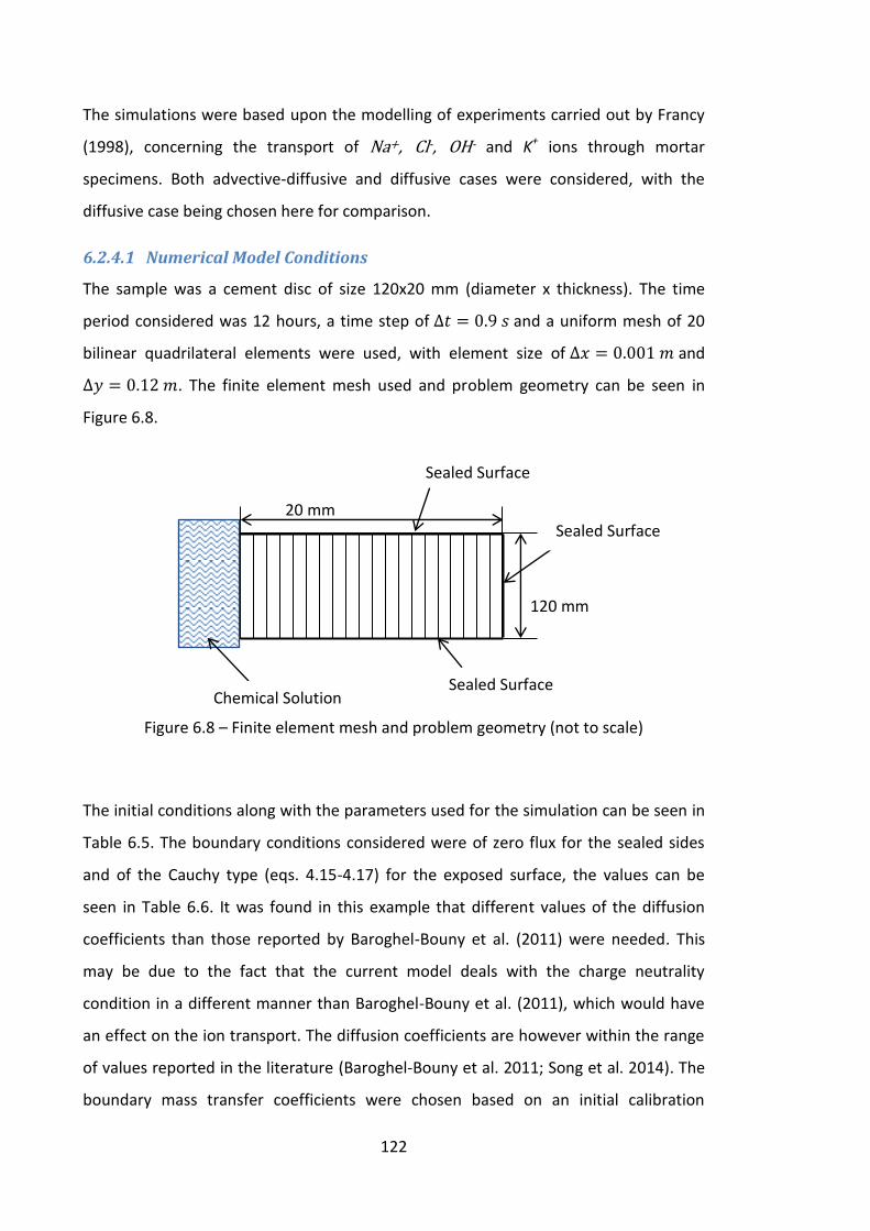
122
The simulations were based upon the modelling of experiments carried out by Francy
(1998), concerning the transport of Na+, Cl-, OH- and K+ ions through mortar
specimens. Both advective-diffusive and diffusive cases were considered, with the
diffusive case being chosen here for comparison.
6.2.4.1 Numerical Model Conditions
The sample was a cement disc of size 120x20 mm (diameter x thickness). The time
period considered was 12 hours, a time step of and a uniform mesh of 20
bilinear quadrilateral elements were used, with element size of and
. The finite element mesh used and problem geometry can be seen in
Figure 6.8.
Figure 6.8 – Finite element mesh and problem geometry (not to scale)
The initial conditions along with the parameters used for the simulation can be seen in
Table 6.5. The boundary conditions considered were of zero flux for the sealed sides
and of the Cauchy type (eqs. 4.15-4.17) for the exposed surface, the values can be
seen in Table 6.6. It was found in this example that different values of the diffusion
coefficients than those reported by Baroghel-Bouny et al. (2011) were needed. This
may be due to the fact that the current model deals with the charge neutrality
condition in a different manner than Baroghel-Bouny et al. (2011), which would have
an effect on the ion transport. The diffusion coefficients are however within the range
of values reported in the literature (Baroghel-Bouny et al. 2011; Song et al. 2014). The
boundary mass transfer coefficients were chosen based on an initial calibration
20 mm
120 mm
Chemical Solution Sealed Surface
Sealed Surface
Sealed Surface

123
exercise (which involved changing the values on a trial and error basis until a good
match was obtained).
Table 6.5 – Model parameters
Parameter Values
Porosity na 0.13
Boundary (eqs. 4.15-
4.17)
(W/Km2) 8.0
(10-3 m/s) 6.5
Initial Values Swa 1.0
Tcca (kg/kg) 0.01954
Na+a(kg/kg) 0.01352
Cl-a(kg/kg) 0.01954
OH-a(kg/kg) 0.00188
K+a(kg/kg) 0.00319
Reaction (eqs. 3.39 &
6.2)
kdaa (10-4) 1.305
λa 0.61
δa 2
a(mol/dm3) 21
Diffusion (eq. 3.38)
Dmol (10-10 m2/s)
Na+ 1.33
Cl- 2.1
OH- 5.3
K+ 1.96 aTaken from (Baroghel-Bouny et al. 2011)
Table 6.6 –Boundary conditions
Boundary Boundary Type Values
LHS Cauchy RH=100 %, T=293 K, Na+=0.000299 kg/kg,
Cl-=0.0 kg/kg, OH-=0.001105 kg/kg, K+=0.002028 kg/kg
Bottom Sealed -
RHS Sealed -
Top Sealed -
6.2.4.2 Results and Discussions
The comparison of the results of the model and the results of Baroghel-Bouny et al.
(2011) can be seen in Figure 6.9.
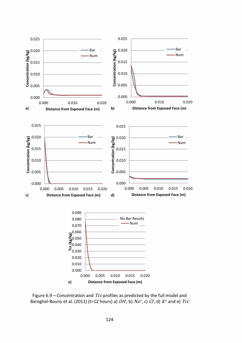
124
Figure 6.9 – Concentration and Tcc profiles as predicted by the full model and Baroghel-Bouny et al. (2011) (t=12 hours) a) OH-, b) Na+, c) Cl-, d) K+ and e) Tcc
0.000
0.005
0.010
0.015
0.020
0.025
0.000 0.010 0.020
Co
nce
ntr
atio
n (
kg/k
g)
Distance from Exposed Face (m) a)
Bar
Num
0.000
0.005
0.010
0.015
0.020
0.025
0.000 0.010 0.020
Co
nce
ntr
atio
n (
kg/k
g)
Distance from Exposed Face (m) b)
Bar
Num
0.000
0.005
0.010
0.015
0.020
0.025
0.000 0.005 0.010 0.015 0.020
Co
nce
ntr
atio
n (
kg/k
g)
Distance from Exposed Face (m) c)
Bar
Num
0.000
0.005
0.010
0.015
0.020
0.025
0.000 0.005 0.010 0.015 0.020
Co
nce
ntr
atio
n (
kg/k
g)
Distance from Exposed Face (m) d)
Bar
Num
0.000
0.010
0.020
0.030
0.040
0.050
0.060
0.070
0.080
0.090
0.000 0.005 0.010 0.015 0.020
Tcc
(kg/
kg)
Distance from Exposed Face (m) e)
NumNo Bar Results
125
In can be seen from the profiles above that the model predictions are in good
agreement with the simulations of Baroghel-Bouny et al. (2011), with the biggest
differences being the slight over prediction of the Na+ concentration near the exposed
face and the under prediction of OH- concentration near the peak that has arisen as a
result of the chloride binding.
6.2.5 Example – Song et al. (2014)
In 2014 Song et al. (2014) developed a model to simulate the chloride transport in
multiple-ionic solutions in cementitious materials, supplemented by experimental
diffusion tests. It is the numerical simulations that are considered here as they provide
results for all the chemical species and sorbed masses considered, whereas the
experimental results concern only the total chloride content. The simulation
considered the diffusion of chemical ions into a concrete specimen, the pore solution
of which had an initial composition which included the presence of a number of ions,
namely, Na+, Ca2+, K+, OH- and SO42-. Two different scenarios were modelled, one of a
NaCl source solution and the other of a CaCl2 source solution. The results of the CaCl2
source solution case were considered here. A number of different reactions were
considered in the model, including the dissolution of portlandite, and the dissolution of
calcium and hydroxide from the C-S-H phases. The chemical chloride bindings onto the
AFm phases were also considered, including formation of both Friedel’s salt and
Kuzel’s salt. The physical absorption of the chloride ions onto the C-S-H phases was
also taken into account, however their chemical binding onto the same phase was not
considered. Finally the alkali bindings onto both the C-S-H and Afm phases were
included. All of the reactions were considered with an assumption of non-equilibrium
conditions and can be described using a Freundlich type isotherm, the rates of which
are empirical but based on mass action law or empirical equations similar to mass
action law. These reactions are given as:
[ ](
([ ][ ] ) ) (6.3)
[ ]
([ ][ ] ) (6.4)
[ ]
([ ][ ] ) (6.5)
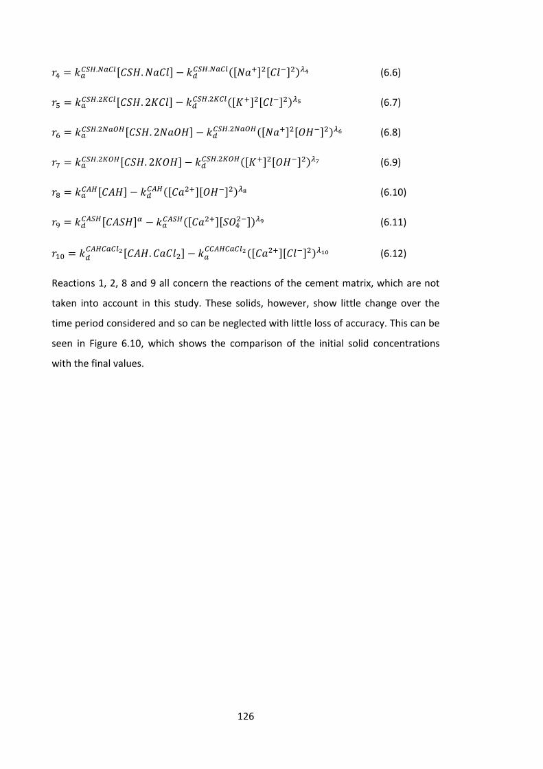
126
[ ]
([ ] [ ] ) (6.6)
[ ]
([ ] [ ] ) (6.7)
[ ]
([ ] [ ] ) (6.8)
[ ]
([ ] [ ] ) (6.9)
[ ]
([ ][ ] ) (6.10)
[ ]
([ ][ ]) (6.11)
[ ]
([ ][ ] ) (6.12)
Reactions 1, 2, 8 and 9 all concern the reactions of the cement matrix, which are not
taken into account in this study. These solids, however, show little change over the
time period considered and so can be neglected with little loss of accuracy. This can be
seen in Figure 6.10, which shows the comparison of the initial solid concentrations
with the final values.
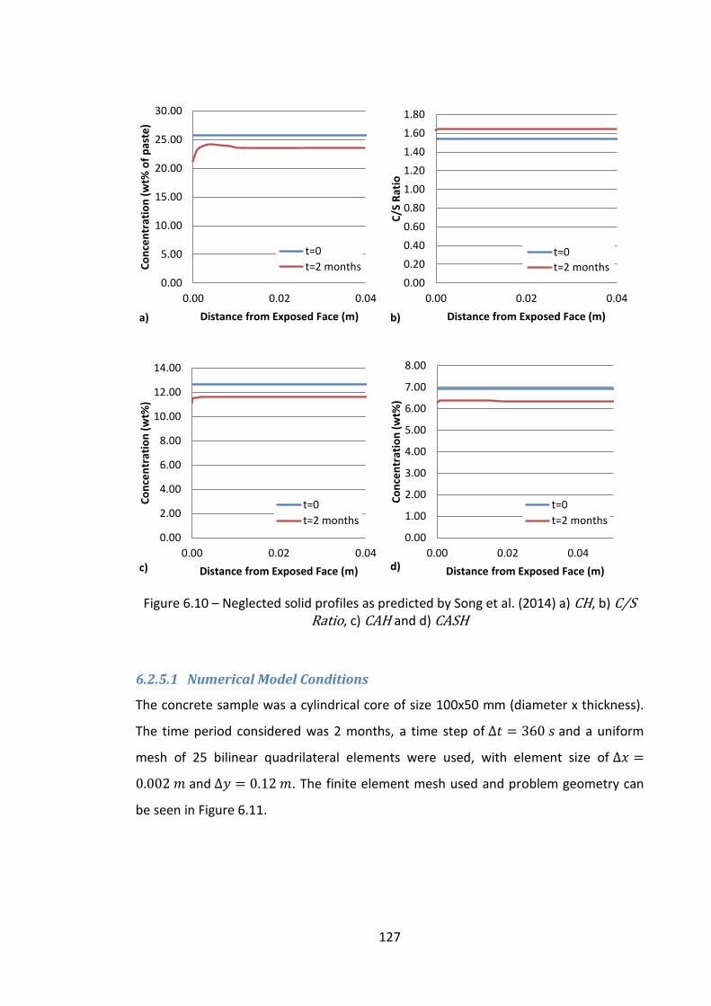
127
Figure 6.10 – Neglected solid profiles as predicted by Song et al. (2014) a) CH, b) C/S
Ratio, c) CAH and d) CASH
6.2.5.1 Numerical Model Conditions
The concrete sample was a cylindrical core of size 100x50 mm (diameter x thickness).
The time period considered was 2 months, a time step of and a uniform
mesh of 25 bilinear quadrilateral elements were used, with element size of
and . The finite element mesh used and problem geometry can
be seen in Figure 6.11.
0.00
5.00
10.00
15.00
20.00
25.00
30.00
0.00 0.02 0.04
Co
nce
ntr
atio
n (
wt%
of
pas
te)
Distance from Exposed Face (m) a)
t=0
t=2 months
0.00
0.20
0.40
0.60
0.80
1.00
1.20
1.40
1.60
1.80
0.00 0.02 0.04
C/S
Rat
io
Distance from Exposed Face (m) b)
t=0
t=2 months
0.00
2.00
4.00
6.00
8.00
10.00
12.00
14.00
0.00 0.02 0.04
Co
nce
ntr
atio
n (
wt%
)
Distance from Exposed Face (m) c)
t=0
t=2 months
0.00
1.00
2.00
3.00
4.00
5.00
6.00
7.00
8.00
0.00 0.02 0.04
Co
nce
ntr
atio
n (
wt%
)
Distance from Exposed Face (m) d)
t=0
t=2 months
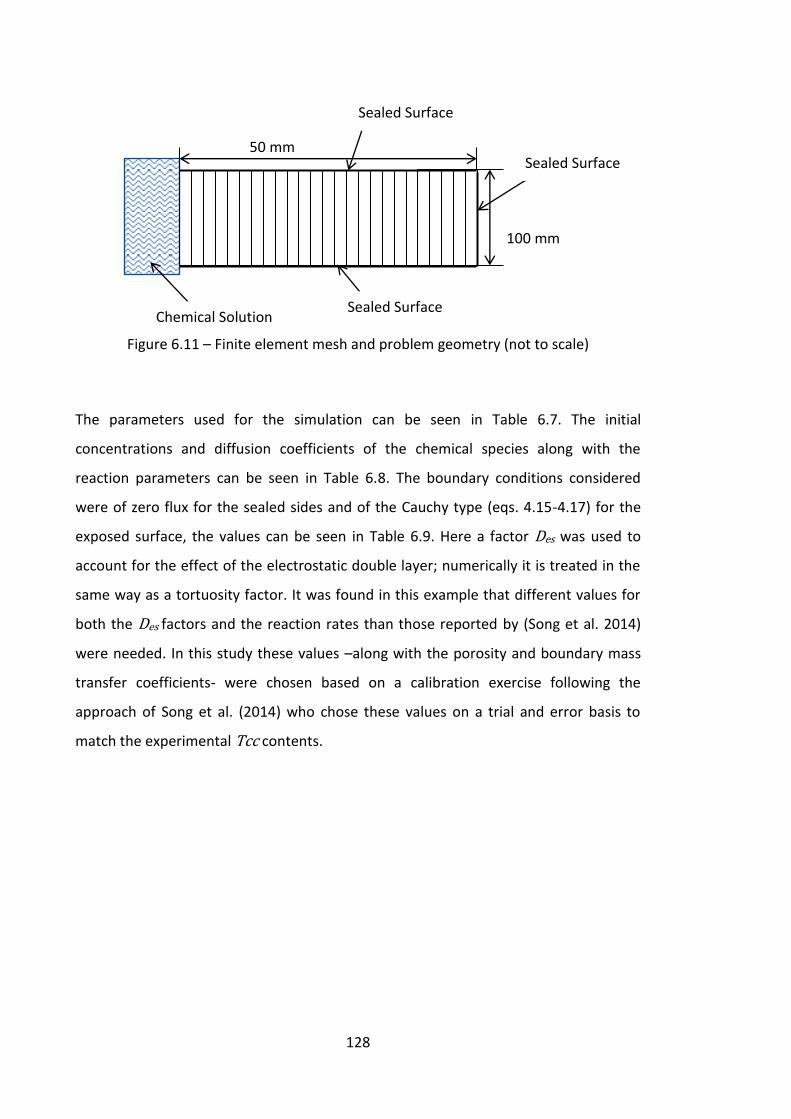
128
Figure 6.11 – Finite element mesh and problem geometry (not to scale)
The parameters used for the simulation can be seen in Table 6.7. The initial
concentrations and diffusion coefficients of the chemical species along with the
reaction parameters can be seen in Table 6.8. The boundary conditions considered
were of zero flux for the sealed sides and of the Cauchy type (eqs. 4.15-4.17) for the
exposed surface, the values can be seen in Table 6.9. Here a factor Des was used to
account for the effect of the electrostatic double layer; numerically it is treated in the
same way as a tortuosity factor. It was found in this example that different values for
both the Des factors and the reaction rates than those reported by (Song et al. 2014)
were needed. In this study these values –along with the porosity and boundary mass
transfer coefficients- were chosen based on a calibration exercise following the
approach of Song et al. (2014) who chose these values on a trial and error basis to
match the experimental Tcc contents.
50 mm
100 mm
Chemical Solution
Sealed Surface
Sealed Surface
Sealed Surface
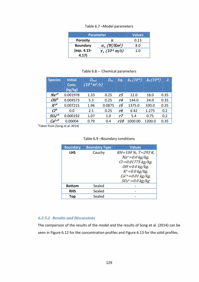
129
Table 6.7 –Model parameters
Parameter Values
Porosity n 0.13
Boundary (eqs. 4.15-
4.17)
(W/Km2) 8.0
(10-4 m/s) 1.0
Table 6.8 – Chemical parameters
Species Initial Conc.
(kg/kg)
Dmol
(10-9 m2/s) Des Eq. ka (10-8) kd (10-8) λ
Na+a 0.001978 1.33 0.25 r3 12.0 18.0 0.35
OH-a 0.004573 5.3 0.25 r4 144.0 24.0 0.35
K+a 0.007215 1.96 0.0875 r5 1375.0 330.0 0.35
Cl-a 0.0 2.1 0.25 r6 6.42 1.275 0.2
SO42-a 0.000192 1.07 1.0 r7 5.4 0.75 0.2
Ca2+a 0.00004 0.79 0.4 r10 1000.00 1200.0 0.35 aTaken from (Song et al. 2014)
Table 6.9 –Boundary conditions
Boundary Boundary Type Values
LHS Cauchy RH=100 %, T=293 K, Na+=0.0 kg/kg,
Cl-=0.01775 kg/kg, OH-=0.0 kg/kg, K+=0.0 kg/kg,
Ca2+=0.01 kg/kg, SO42-=0.0 kg/kg
Bottom Sealed -
RHS Sealed -
Top Sealed -
6.2.5.2 Results and Discussions
The comparison of the results of the model and the results of Song et al. (2014) can be
seen in Figure 6.12 for the concentration profiles and Figure 6.13 for the solid profiles.
130
Figure 6.12 – Concentration profiles as predicted by the full model and Song et al. (2014) (t=2 months) a) Na+, b) K+, c) Ca2+, d) Cl-, e) OH- and f) SO42-
0.0000
0.0005
0.0010
0.0015
0.0020
0.0025
0.00 0.02 0.04
Co
nce
ntr
atio
n (
kg/k
g)
Distance from Exposed Face (m) a)
Song
Num0.000
0.001
0.002
0.003
0.004
0.005
0.006
0.007
0.008
0.00 0.02 0.04
Co
nce
ntr
atio
n (
kg/k
g)
Distance from Exposed Face (m) b)
Song
Num
0.000
0.002
0.004
0.006
0.008
0.010
0.012
0.00 0.02 0.04
Co
nce
ntr
atio
n (
kg/k
g)
Distance from Exposed Face (m) c)
Song
Num
0.000
0.002
0.004
0.006
0.008
0.010
0.012
0.014
0.016
0.018
0.020
0.00 0.02 0.04
Co
nce
ntr
atio
n (
kg/k
g)
Distance from Exposed Face (m) d)
Song
Num
0.0000
0.0005
0.0010
0.0015
0.0020
0.0025
0.0030
0.0035
0.0040
0.0045
0.0050
0.00 0.02 0.04
Co
nce
ntr
atio
n (
kg/k
g)
Distance from Exposed Face (m) e)
Song
Num0.00000
0.00005
0.00010
0.00015
0.00020
0.00025
0.00 0.02 0.04
Co
nce
ntr
atio
n (
kg/k
g)
Distance from Exposed Face (m) f)
Song
Num
131
Figure 6.13 – Solid mass profiles as predicted by the full model and Song et al. (2014) (t=2 months) a) CSH.CaCl2, b) CSH.NaCl, c) CSH.2KCl, d) CSH.NaOH, e) CSH.2KCl and
f) CAH.CaCl2
0.00
0.05
0.10
0.15
0.20
0.25
0.30
0.35
0.40
0.45
0.00 0.02 0.04
Cl C
on
cen
trat
ion
(w
t%)
Distance from Exposed Face (m) a)
Song
Num
0.000
0.001
0.002
0.003
0.004
0.005
0.006
0.007
0.00 0.02 0.04
Cl C
on
cen
trat
ion
(w
t%)
Distance from Exposed Face (m) b)
Song
Num
0.000
0.002
0.004
0.006
0.008
0.010
0.012
0.014
0.016
0.018
0.020
0.00 0.02 0.04
Cl C
on
cen
trat
ion
(w
t%)
Distance from Exposed Face (m) c)
Song
Num
0.00
0.02
0.04
0.06
0.08
0.10
0.12
0.00 0.02 0.04
Co
nce
ntr
atio
n (
wt%
)
Distance from Exposed Face (m) d)
Song
Num
0.00
0.02
0.04
0.06
0.08
0.10
0.12
0.14
0.00 0.02 0.04
Co
nce
ntr
atio
n (
wt%
)
Distance from Exposed Face (m) e)
Song
Num0.00
0.10
0.20
0.30
0.40
0.50
0.60
0.00 0.02 0.04
Cl C
on
cen
trat
ion
(w
t%)
Distance from Exposed Face (m) f)
Song
Num
132
It can be seen from the profiles in Figure 6.12 that the model predictions are generally
in good agreement with the simulations of Song et al. (2014), with the Ca2+ and Cl-
being almost identical. The diffusion of Na+ is slightly over predicted near the exposed
face whereas the diffusion of K+ is under predicted from about 0.006 m to 0.03 m. The
amount of transport of both OH- and SO42- is in agreement but the shapes of the
curves are different, with the results of Song et al. (2014) showing a sharper
concentration front.
The solid mass profiles also show a generally good agreement withCSH.CaCl2 and
CAH.CaCl2 being the closest but slightly over predicted. The CSH.2KOH and CSH.2KCl
are also both in good agreement but slightly under predicted and over predicted
respectively. The CSH.2NaOH profile is similar to the OH- and SO42- profiles in that it is
over predicted in some areas and under predicted in others. In the case of the
CSH.NaCl the penetration is over predicted by the model. It is thought that the
differences in predicted profiles are a result of the following factors:
1. Different numerical methods were used (finite element method vs finite
difference method).
2. Charge neutrality was dealt with in a different way.
3. Reactions, 1,2, 8 and 9 were neglected in this study, but may have had a
significant effect on certain profiles (for example SO42- which is involved in
reaction 9 and may be sensitive to small changes due to its low concentration).
6.3 Validation of the Coupled Model
6.3.1 Introduction
This section deals with validation of the moisture flow and chemical transport part of
the model and involves the numerical simulation of experimental results carried out on
the drying of cementitious materials by Kim and Lee (1999) and of the ion transport
experiments reported in Chapter 5.
For both examples the mesh and time step sizes were chosen based on the results of a
mesh convergence study.
133
6.3.2 Example – Kim and Lee (1999)
Kim and Lee (1999) reported results of an experimental study and numerical modelling
of moisture diffusion and self-desiccation in concrete specimens. The results of the
experimental study are used here to allow validation of the model developed in
Chapter 4. Three different concrete mixes were considered, a high strength (H),
medium strength (M) and a low strength (L). The materials used were ordinary
Portland cement, river sand and crushed granite gravel of size <19 mm. The mix
proportions for the three different mixes can be seen in Table 6.10 (reproduced from
Kim and Lee (1999)).
Table 6.10 – Mix parameters
Mix w/c F.A./C.A. Water (kg/m3)
Cement (kg/m3)
F.A. (kg/m3)
C.A. (kg/m3)
S.P. (Cx%)
fc (MPa)
H 0.28 0.38 151 541 647 1055 2.0 76
M 0.40 0.42 169 423 736 1016 0.5 53
L 0.68 0.45 210 310 782 955 0.0 22
where F.A. stands for the fine aggregate, C.A. stands for the coarse aggregate, S.P.
stands for super plasticiser, and fc is the compressive strength. Once the beam
specimens were cast they were moist cured for 28 days before testing. Following this,
five sides were sealed with paraffin wax, with the remaining side being exposed to an
environmental relative humidity of 50 %. The change in relative humidity was
measured at three positions along the profile of the specimen, namely 3 cm, 7 cm and
12 cm from the exposed face. To take these measurements holes were drilled at the
three locations, into which plastic sleeves were inserted, containing the humidity
probes with a rubber plug, as shown in Figure 6.14. The measurements were taken
using Vaisala HMP44 probes and Vaisala HMI41 indicators. The problem geometry and
the position of the measuring points can be seen in Figure 6.15.
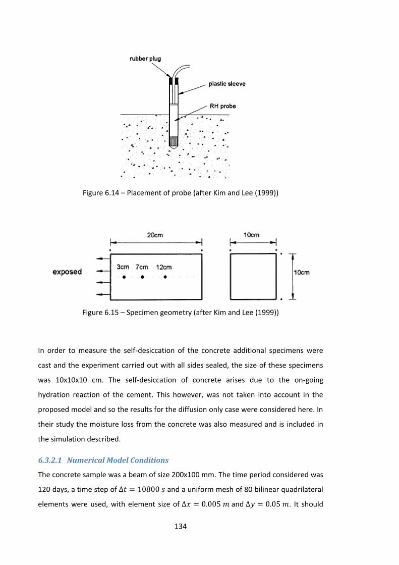
134
Figure 6.14 – Placement of probe (after Kim and Lee (1999))
Figure 6.15 – Specimen geometry (after Kim and Lee (1999))
In order to measure the self-desiccation of the concrete additional specimens were
cast and the experiment carried out with all sides sealed, the size of these specimens
was 10x10x10 cm. The self-desiccation of concrete arises due to the on-going
hydration reaction of the cement. This however, was not taken into account in the
proposed model and so the results for the diffusion only case were considered here. In
their study the moisture loss from the concrete was also measured and is included in
the simulation described.
6.3.2.1 Numerical Model Conditions
The concrete sample was a beam of size 200x100 mm. The time period considered was
120 days, a time step of and a uniform mesh of 80 bilinear quadrilateral
elements were used, with element size of and . It should
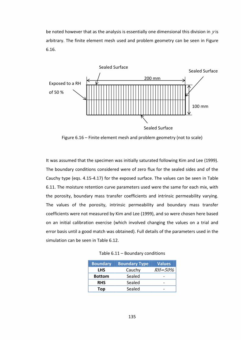
135
be noted however that as the analysis is essentially one dimensional this division in y is
arbitrary. The finite element mesh used and problem geometry can be seen in Figure
6.16.
Figure 6.16 – Finite element mesh and problem geometry (not to scale)
It was assumed that the specimen was initially saturated following Kim and Lee (1999).
The boundary conditions considered were of zero flux for the sealed sides and of the
Cauchy type (eqs. 4.15-4.17) for the exposed surface. The values can be seen in Table
6.11. The moisture retention curve parameters used were the same for each mix, with
the porosity, boundary mass transfer coefficients and intrinsic permeability varying.
The values of the porosity, intrinsic permeability and boundary mass transfer
coefficients were not measured by Kim and Lee (1999), and so were chosen here based
on an initial calibration exercise (which involved changing the values on a trial and
error basis until a good match was obtained). Full details of the parameters used in the
simulation can be seen in Table 6.12.
Table 6.11 – Boundary conditions
Boundary Boundary Type Values
LHS Cauchy RH=50% Bottom Sealed -
RHS Sealed -
Top Sealed -
200 mm
100 mm
Exposed to a RH
of 50 %
Sealed Surface
Sealed Surface Sealed Surface
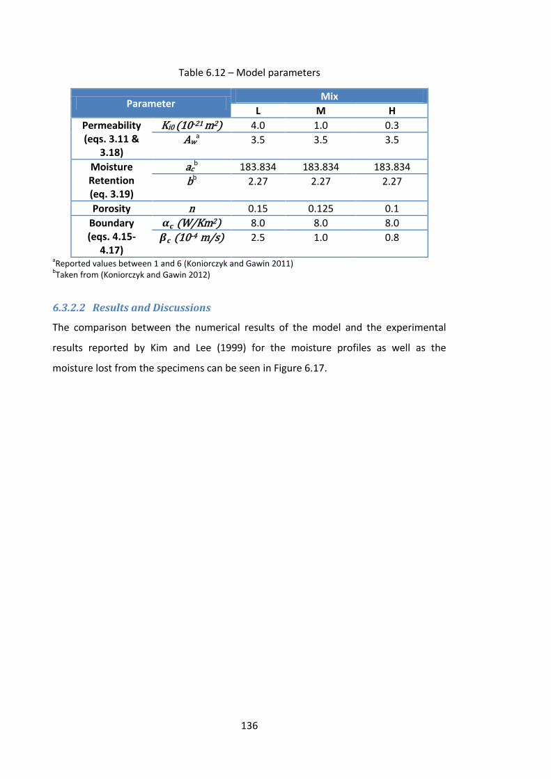
136
Table 6.12 – Model parameters
Parameter Mix
L M H
Permeability (eqs. 3.11 &
3.18)
Ki0 (10-21 m2) 4.0 1.0 0.3
Awa 3.5 3.5 3.5
Moisture Retention (eq. 3.19)
acb 183.834 183.834 183.834
bb 2.27 2.27 2.27
Porosity n 0.15 0.125 0.1
Boundary (eqs. 4.15-
4.17)
(W/Km2) 8.0 8.0 8.0
(10-4 m/s) 2.5 1.0 0.8
aReported values between 1 and 6 (Koniorczyk and Gawin 2011)
bTaken from (Koniorczyk and Gawin 2012)
6.3.2.2 Results and Discussions
The comparison between the numerical results of the model and the experimental
results reported by Kim and Lee (1999) for the moisture profiles as well as the
moisture lost from the specimens can be seen in Figure 6.17.
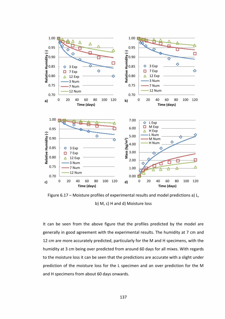
137
Figure 6.17 – Moisture profiles of experimental results and model predictions a) L,
b) M, c) H and d) Moisture loss
It can be seen from the above figure that the profiles predicted by the model are
generally in good agreement with the experimental results. The humidity at 7 cm and
12 cm are more accurately predicted, particularly for the M and H specimens, with the
humidity at 3 cm being over predicted from around 60 days for all mixes. With regards
to the moisture loss it can be seen that the predictions are accurate with a slight under
prediction of the moisture loss for the L specimen and an over prediction for the M
and H specimens from about 60 days onwards.
0.70
0.75
0.80
0.85
0.90
0.95
1.00
0 20 40 60 80 100 120
Re
lati
ve H
um
idit
y (-
)
Time (days) a)
3 Exp
7 Exp
12 Exp
3 Num
7 Num
12 Num0.70
0.75
0.80
0.85
0.90
0.95
1.00
0 20 40 60 80 100 120
Re
lati
ve H
um
idit
y (-
)
Time (days) b)
3 Exp
7 Exp
12 Exp
3 Num
7 Num
12 Num
0.70
0.75
0.80
0.85
0.90
0.95
1.00
0 20 40 60 80 100 120
Re
lati
ve H
um
idit
y (-
)
Time (days) c)
3 Exp
7 Exp
12 Exp
3 Num
7 Num
12 Num0.00
1.00
2.00
3.00
4.00
5.00
6.00
7.00
0 20 40 60 80 100 120
Mas
s (k
g/m
2)
Time (days) d)
L ExpM ExpH ExpL NumM NumH Num
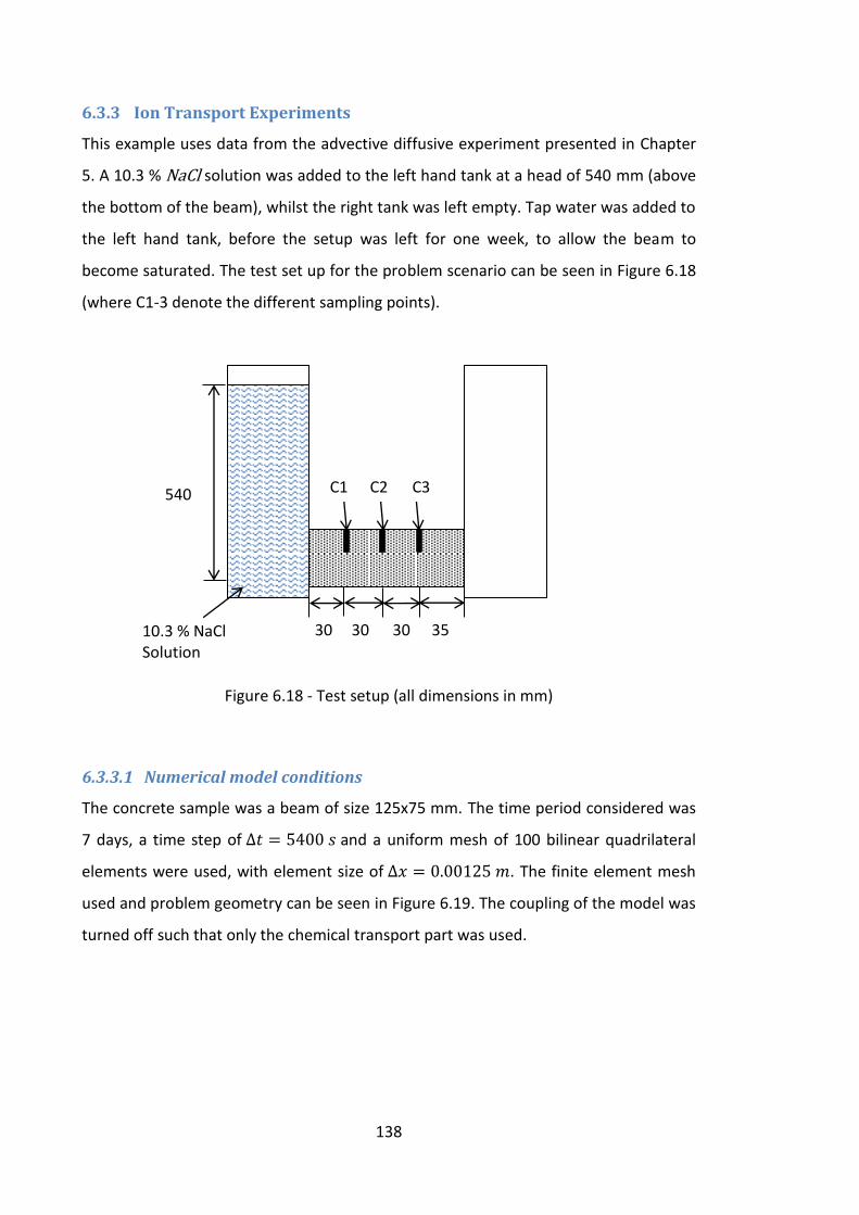
138
6.3.3 Ion Transport Experiments
This example uses data from the advective diffusive experiment presented in Chapter
5. A 10.3 % NaCl solution was added to the left hand tank at a head of 540 mm (above
the bottom of the beam), whilst the right tank was left empty. Tap water was added to
the left hand tank, before the setup was left for one week, to allow the beam to
become saturated. The test set up for the problem scenario can be seen in Figure 6.18
(where C1-3 denote the different sampling points).
Figure 6.18 - Test setup (all dimensions in mm)
6.3.3.1 Numerical model conditions
The concrete sample was a beam of size 125x75 mm. The time period considered was
7 days, a time step of and a uniform mesh of 100 bilinear quadrilateral
elements were used, with element size of . The finite element mesh
used and problem geometry can be seen in Figure 6.19. The coupling of the model was
turned off such that only the chemical transport part was used.
10.3 % NaCl Solution
30 30 30 35
540 C1 C2 C3
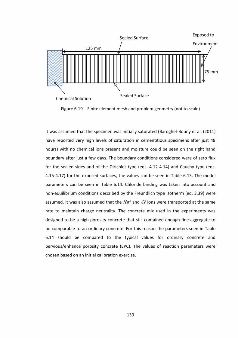
139
Figure 6.19 – Finite element mesh and problem geometry (not to scale)
It was assumed that the specimen was initially saturated (Baroghel-Bouny et al. (2011)
have reported very high levels of saturation in cementitious specimens after just 48
hours) with no chemical ions present and moisture could be seen on the right hand
boundary after just a few days. The boundary conditions considered were of zero flux
for the sealed sides and of the Dirichlet type (eqs. 4.12-4.14) and Cauchy type (eqs.
4.15-4.17) for the exposed surfaces, the values can be seen in Table 6.13. The model
parameters can be seen in Table 6.14. Chloride binding was taken into account and
non-equilibrium conditions described by the Freundlich type isotherm (eq. 3.39) were
assumed. It was also assumed that the Na+ and Cl- ions were transported at the same
rate to maintain charge neutrality. The concrete mix used in the experiments was
designed to be a high porosity concrete that still contained enough fine aggregate to
be comparable to an ordinary concrete. For this reason the parameters seen in Table
6.14 should be compared to the typical values for ordinary concrete and
pervious/enhance porosity concrete (EPC). The values of reaction parameters were
chosen based on an initial calibration exercise.
75 mm
Chemical Solution Sealed Surface
125 mm
Sealed Surface Exposed to
Environment
140
Table 6.13 – Boundary conditions
Boundary Boundary Type Values
LHS Dirichlet cCl=0.063 kg/kg, cNa=0.041 kg/kg
Bottom Sealed -
RHS Cauchy cCl=0.0 kg/kg, cNa=0.0 kg/kg
Top Sealed -
Table 6.14 – Model parameters
Variable Value
na 0.20
Ki0b
(10-16 m2) 6.59
Dmolc (10-10 m2/s) 2.1
kda (10-5) 1.305
λ 1.9 aReported values of 0.10-0.13 (Baroghel-Bouny et al. 2011) and 0.16-0.264 for EPC (Neithalath et al.
2006) bReported values of the order 10
-21m
2 (Baroghel-Bouny et al. 2011) and 10
-10m
2 for EPC (Neithalath et al.
2006) cReported values of 2.1x10
-9m
2/s (Song et al. 2014) to 2.1x10
-12m
2/s (Baroghel-Bouny et al. 2011)
6.3.3.2 Results and discussions
The Cl- and Na+ profiles as measured from the experiment and predicted from the
model after one week can be seen in Figure 6.20. It can be noted that due to the
significant problems encountered with the experimental set up leaking these are the
only set of viable results obtained.
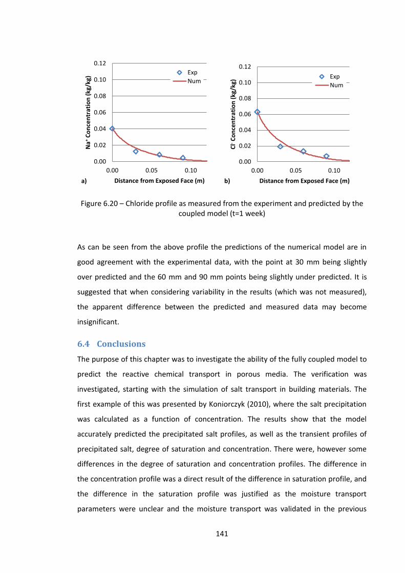
141
Figure 6.20 – Chloride profile as measured from the experiment and predicted by the coupled model (t=1 week)
As can be seen from the above profile the predictions of the numerical model are in
good agreement with the experimental data, with the point at 30 mm being slightly
over predicted and the 60 mm and 90 mm points being slightly under predicted. It is
suggested that when considering variability in the results (which was not measured),
the apparent difference between the predicted and measured data may become
insignificant.
6.4 Conclusions
The purpose of this chapter was to investigate the ability of the fully coupled model to
predict the reactive chemical transport in porous media. The verification was
investigated, starting with the simulation of salt transport in building materials. The
first example of this was presented by Koniorczyk (2010), where the salt precipitation
was calculated as a function of concentration. The results show that the model
accurately predicted the precipitated salt profiles, as well as the transient profiles of
precipitated salt, degree of saturation and concentration. There were, however some
differences in the degree of saturation and concentration profiles. The difference in
the concentration profile was a direct result of the difference in saturation profile, and
the difference in the saturation profile was justified as the moisture transport
parameters were unclear and the moisture transport was validated in the previous
0.00
0.02
0.04
0.06
0.08
0.10
0.12
0.00 0.05 0.10
Na+
Co
nce
ntr
atio
n (
kg/k
g)
Distance from Exposed Face (m) a)
Exp
Num
0.00
0.02
0.04
0.06
0.08
0.10
0.12
0.00 0.05 0.10
Cl- C
on
cen
trat
ion
(kg
/kg)
Distance from Exposed Face (m) b)
Exp
Num
142
example. The second example was presented by Koniorczyk and Gawin (2012), where
the salt precipitation was calculated as a function of solution supersaturation profile.
The results showed good agreement between the model and the results from
Koniorczyk and Gawin (2012), with the biggest difference being found in the transient
profile of solution supersaturation ratio.
The next two examples investigated the ability of the model to predict multi-ionic
transport. The first example of this was presented by Baroghel-Bouny et al. (2011) and
concerned the transport of four chemical ions into a mortar specimen. The resultant
profiles were in good agreement with a slight over prediction of the Na+ concentration
near the exposed face and a slight under prediction of the OH- concentration near the
peak value caused by the reaction. The final example was presented by Song et al.
(2014) and concerned the transport of six chemical ions in a concrete specimen and six
different chemical reactions. The results showed good agreement between the model
and the results presented by Song et al. with the Ca2+ and Cl- being almost identical.
The worst prediction was of the CSH.NaCl profile where the penetration is over
predicted by the model.
The validation of the moisture transport was then investigated through the simulation
of drying experiments carried out by Kim and Lee (1999). It was found that the model
accurately predicted the moisture profiles at 7 cm and 12 cm for all three mixes, as
well as the moisture loss for the L specimen. The profiles at 3 cm were under predicted
from around 60 days onwards, whilst the moisture loss for the M and H specimen was
slightly over predicted from 60 days onwards. The validation of the chemical transport
was investigated through the simulation of the results of the ion transport
experiments; it was found that the model performed well in matching the
concentration profiles.
It has been shown in this chapter that the developed model can accurately capture the
chemical behaviour in porous media including moisture transport, multi-ionic chemical
transport and chemical reactions.
143
Chapter 7. Applicability Investigation and Verification of the
Problem Reduction Scheme
7.1 Introduction
In this chapter the performance of the problem reduction schemes is examined. This is
split into two parts; first, each of the problem reduction schemes are tested to
determine their range of applicability, using a hypothetical example problem
concerning the reactive transport of 16 chemical species; secondly, the schemes are
verified against a series of numerical simulations taken from, or based on, examples in
the literature.
Section 7.2 describes an investigation into the range of applicability of each reduction
schemes. As part of this study, the degree to which each PRS maintains mass balance is
examined.
The verification of the PRSs is then presented in section 7.3, where each PRS is
compared to an example problem taken from the literature and the accuracy of the
predictions are discussed.
Section 7.4 presents the results of the reduction in computational cost achieved by the
PRSs in terms of CPU time.
Section 7.5 details an investigation into the use of analytical relationships for the
reduction scheme and the problems encountered.
Finally, in Section 7.6, a set of conclusions are drawn from the work on the calibration
and performance of the PRSs.
7.2 Applicability Investigation of Reduction Schemes
The three reduction approaches presented will have different ranges of applicability in
terms of the diffusion coefficient range over which they will give an acceptable
approximation. It is expected that PRS 1 will be accurate over the smallest diffusion
coefficient range as the transport is extrapolated as a multiple of the indicator species,
whereas PRS 2 and 3 bound the solution using indicator species at either end of the
diffusion coefficient range. The interpolation/extrapolation equations used to predict
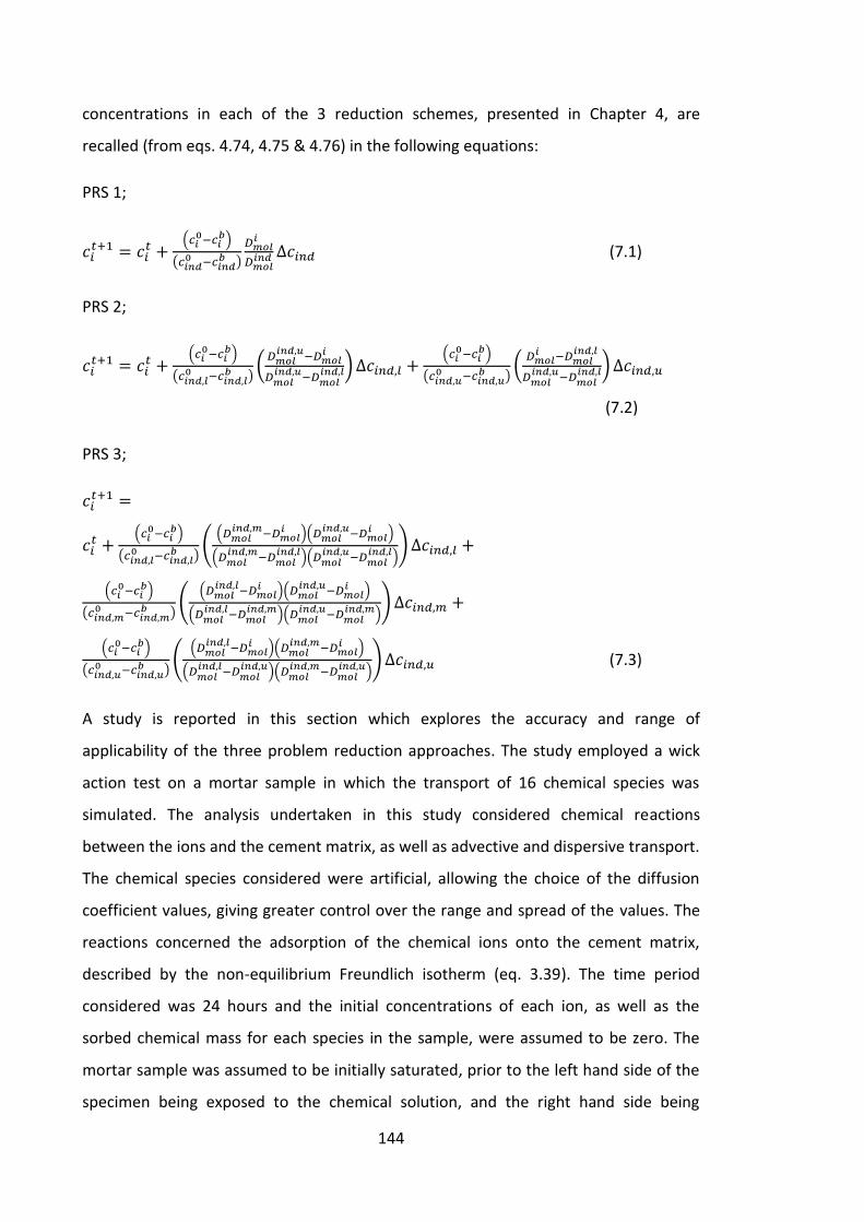
144
concentrations in each of the 3 reduction schemes, presented in Chapter 4, are
recalled (from eqs. 4.74, 4.75 & 4.76) in the following equations:
PRS 1;
(
)
(
)
(7.1)
PRS 2;
(
)
( , ,
)(
,
,
, ) , (
)
( , ,
)(
,
,
, ) ,
(7.2)
PRS 3;
(
)
( , ,
)(
( ,
)( ,
)
( ,
, )( ,
, )) ,
(
)
( , ,
)(
( ,
)( ,
)
( ,
, )( ,
, )) ,
(
)
( , ,
)(
( ,
)( ,
)
( ,
, )( ,
, )) , (7.3)
A study is reported in this section which explores the accuracy and range of
applicability of the three problem reduction approaches. The study employed a wick
action test on a mortar sample in which the transport of 16 chemical species was
simulated. The analysis undertaken in this study considered chemical reactions
between the ions and the cement matrix, as well as advective and dispersive transport.
The chemical species considered were artificial, allowing the choice of the diffusion
coefficient values, giving greater control over the range and spread of the values. The
reactions concerned the adsorption of the chemical ions onto the cement matrix,
described by the non-equilibrium Freundlich isotherm (eq. 3.39). The time period
considered was 24 hours and the initial concentrations of each ion, as well as the
sorbed chemical mass for each species in the sample, were assumed to be zero. The
mortar sample was assumed to be initially saturated, prior to the left hand side of the
specimen being exposed to the chemical solution, and the right hand side being
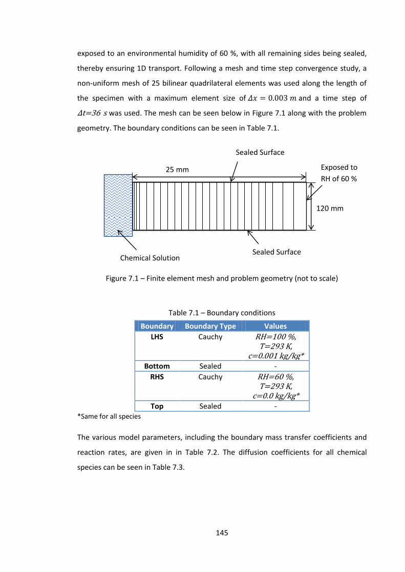
145
exposed to an environmental humidity of 60 %, with all remaining sides being sealed,
thereby ensuring 1D transport. Following a mesh and time step convergence study, a
non-uniform mesh of 25 bilinear quadrilateral elements was used along the length of
the specimen with a maximum element size of and a time step of
t=36 s was used. The mesh can be seen below in Figure 7.1 along with the problem
geometry. The boundary conditions can be seen in Table 7.1.
Figure 7.1 – Finite element mesh and problem geometry (not to scale)
Table 7.1 – Boundary conditions
Boundary Boundary Type Values
LHS Cauchy RH=100 %, T=293 K,
c=0.001 kg/kg* Bottom Sealed -
RHS Cauchy RH=60 %, T=293 K,
c=0.0 kg/kg*
Top Sealed - *Same for all species
The various model parameters, including the boundary mass transfer coefficients and
reaction rates, are given in in Table 7.2. The diffusion coefficients for all chemical
species can be seen in Table 7.3.
25 mm
120 mm
Chemical Solution
Sealed Surface
Sealed Surface
Exposed to
RH of 60 %
146
Table 7.2 – Model parameters
Parameter Value
kda 0.008
λ 2.0
n 0.13
βc (m/s) 2.5x10⁻³
γc (kg/m2s) 1x10⁻⁴
ωc (W/m2K) 8.0
Ki0 (10-21 m2) 35.0
Aw 2.0
Table 7.3 – Chemical parameters
Species Dmol
(10-10 m2/s)
Species (cont’d)
Dmol
(10-10 m2/s)
1 0.25 9 6
2 0.5 10 7
3 1 11 8
4 1.5 12 9
5 2 13 10
6 3 14 12
7 4 15 14
8 5 16 16
To determine the accuracy of the reduction schemes an analysis of the full problem
has been undertaken. Once the results from the full model were obtained, the analysis
could be carried out using each of the problem reduction schemes. The indicator
species chosen for each of the techniques can be seen in Table 7.4. An artificial species
labelled ‘A’ has been chosen for PRS 1 and 2 in order to allow the use of an indicator
with a diffusion coefficient corresponding to the mean value of the species diffusion
coefficients. Artificial indicator species may also be used for other reasons; for
example, PRS 2 and 3 use indicator species with the highest and lowest diffusion
coefficients, bounding the solution; in some cases the upper indicator species may be
highly reactive, meaning that its rate of transport may no longer be the highest. In this
situation, a non-reactive artificial indicator could be used in its place, maintaining the
bounding of the solution.
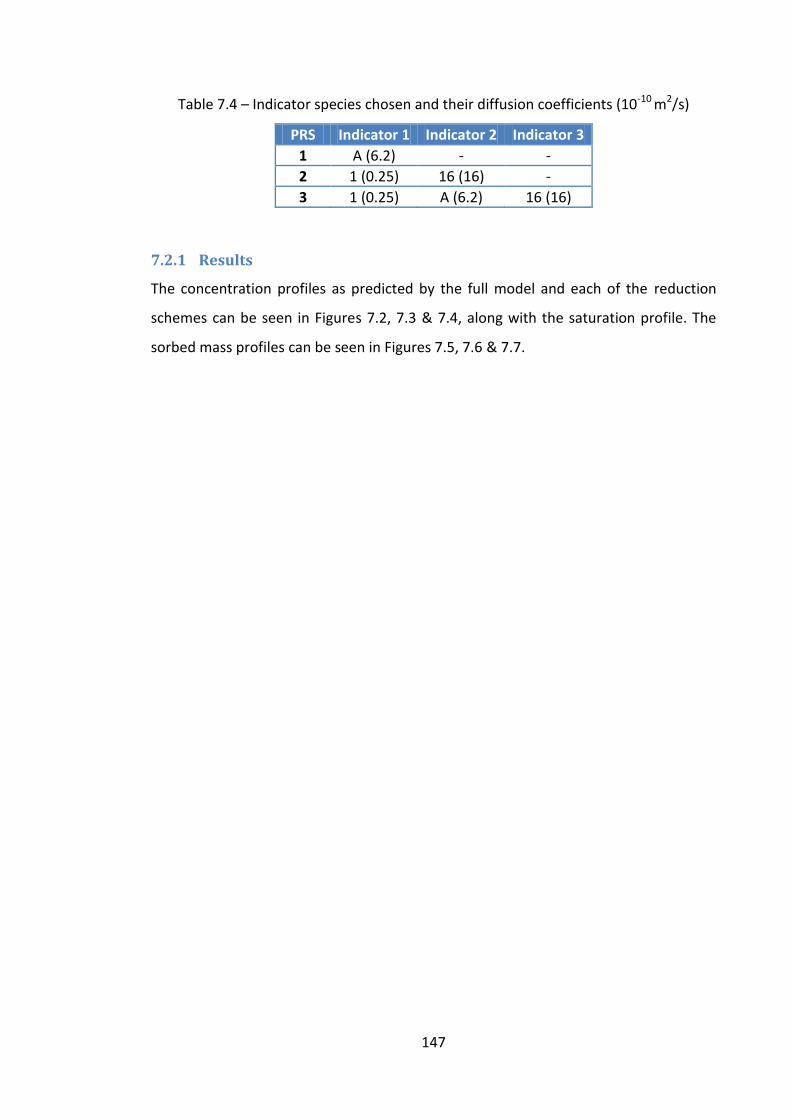
147
Table 7.4 – Indicator species chosen and their diffusion coefficients (10-10 m2/s)
PRS Indicator 1 Indicator 2 Indicator 3
1 A (6.2) - -
2 1 (0.25) 16 (16) -
3 1 (0.25) A (6.2) 16 (16)
7.2.1 Results
The concentration profiles as predicted by the full model and each of the reduction
schemes can be seen in Figures 7.2, 7.3 & 7.4, along with the saturation profile. The
sorbed mass profiles can be seen in Figures 7.5, 7.6 & 7.7.
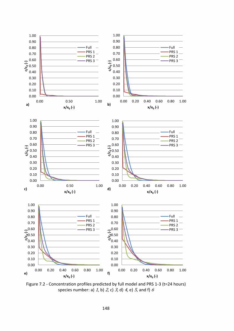
148
Figure 7.2 - Concentration profiles predicted by full model and PRS 1-3 (t=24 hours)
species number: a) 1, b) 2, c) 3, d) 4, e) 5, and f) 6
0.00
0.10
0.20
0.30
0.40
0.50
0.60
0.70
0.80
0.90
1.00
0.00 0.50 1.00
c/c 0
(-)
x/x0 (-) a)
FullPRS 1PRS 2PRS 3
0.00
0.10
0.20
0.30
0.40
0.50
0.60
0.70
0.80
0.90
1.00
0.00 0.20 0.40 0.60 0.80 1.00
c/c 0
(-)
x/x0 (-)
b)
FullPRS 1PRS 2PRS 3
0.00
0.10
0.20
0.30
0.40
0.50
0.60
0.70
0.80
0.90
1.00
0.00 0.50 1.00
c/c 0
(-)
x/x0 (-) c)
FullPRS 1PRS 2PRS 3
0.00
0.10
0.20
0.30
0.40
0.50
0.60
0.70
0.80
0.90
1.00
0.00 0.20 0.40 0.60 0.80 1.00
c/c 0
(-)
x/x0 (-) d)
FullPRS 1PRS 2PRS 3
0.00
0.10
0.20
0.30
0.40
0.50
0.60
0.70
0.80
0.90
1.00
0.00 0.20 0.40 0.60 0.80 1.00
c/c 0
(-)
x/x0 (-) e)
FullPRS 1PRS 2PRS 3
0.00
0.10
0.20
0.30
0.40
0.50
0.60
0.70
0.80
0.90
1.00
0.00 0.20 0.40 0.60 0.80 1.00
c/c 0
(-)
x/x0 (-) f)
FullPRS 1PRS 2PRS 3
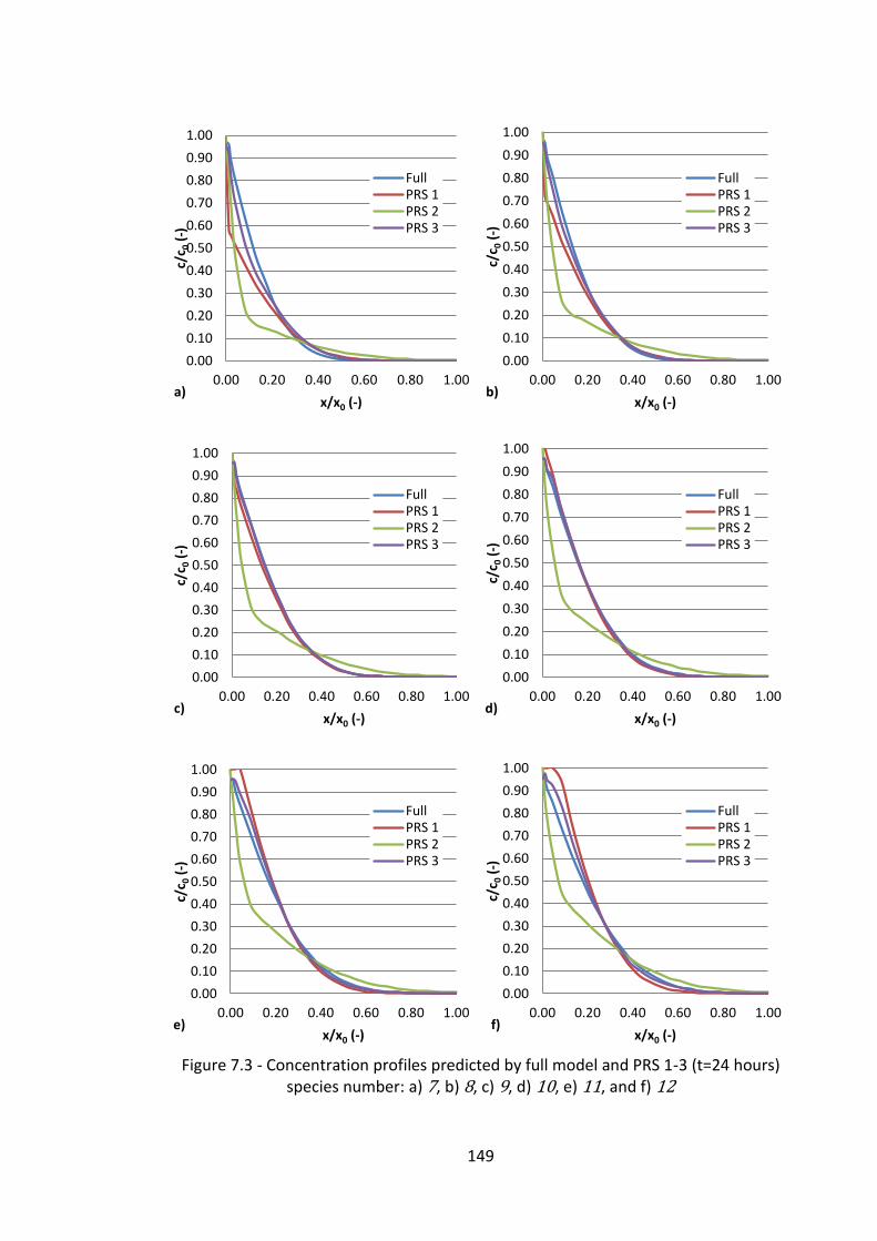
149
Figure 7.3 - Concentration profiles predicted by full model and PRS 1-3 (t=24 hours)
species number: a) 7, b) 8, c) 9, d) 10, e) 11, and f) 12
0.00
0.10
0.20
0.30
0.40
0.50
0.60
0.70
0.80
0.90
1.00
0.00 0.20 0.40 0.60 0.80 1.00
c/c 0
(-)
x/x0 (-) a)
FullPRS 1PRS 2PRS 3
0.00
0.10
0.20
0.30
0.40
0.50
0.60
0.70
0.80
0.90
1.00
0.00 0.20 0.40 0.60 0.80 1.00
c/c 0
(-)
x/x0 (-) b)
FullPRS 1PRS 2PRS 3
0.00
0.10
0.20
0.30
0.40
0.50
0.60
0.70
0.80
0.90
1.00
0.00 0.20 0.40 0.60 0.80 1.00
c/c 0
(-)
x/x0 (-) c)
FullPRS 1PRS 2PRS 3
0.00
0.10
0.20
0.30
0.40
0.50
0.60
0.70
0.80
0.90
1.00
0.00 0.20 0.40 0.60 0.80 1.00
c/c 0
(-)
x/x0 (-) d)
FullPRS 1PRS 2PRS 3
0.00
0.10
0.20
0.30
0.40
0.50
0.60
0.70
0.80
0.90
1.00
0.00 0.20 0.40 0.60 0.80 1.00
c/c 0
(-)
x/x0 (-) e)
FullPRS 1PRS 2PRS 3
0.00
0.10
0.20
0.30
0.40
0.50
0.60
0.70
0.80
0.90
1.00
0.00 0.20 0.40 0.60 0.80 1.00
c/c 0
(-)
x/x0 (-) f)
FullPRS 1PRS 2PRS 3
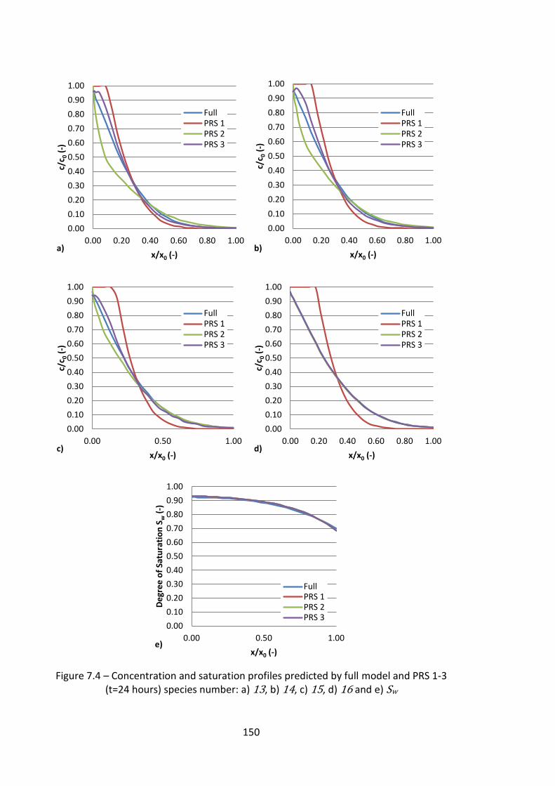
150
Figure 7.4 – Concentration and saturation profiles predicted by full model and PRS 1-3 (t=24 hours) species number: a) 13, b) 14, c) 15, d) 16 and e) Sw
0.00
0.10
0.20
0.30
0.40
0.50
0.60
0.70
0.80
0.90
1.00
0.00 0.20 0.40 0.60 0.80 1.00
c/c 0
(-)
x/x0 (-) a)
FullPRS 1PRS 2PRS 3
0.00
0.10
0.20
0.30
0.40
0.50
0.60
0.70
0.80
0.90
1.00
0.00 0.20 0.40 0.60 0.80 1.00
c/c 0
(-)
x/x0 (-)
b)
FullPRS 1PRS 2PRS 3
0.00
0.10
0.20
0.30
0.40
0.50
0.60
0.70
0.80
0.90
1.00
0.00 0.50 1.00
c/c 0
(-)
x/x0 (-) c)
FullPRS 1PRS 2PRS 3
0.00
0.10
0.20
0.30
0.40
0.50
0.60
0.70
0.80
0.90
1.00
0.00 0.20 0.40 0.60 0.80 1.00
c/c 0
(-)
x/x0 (-) d)
FullPRS 1PRS 2PRS 3
0.00
0.10
0.20
0.30
0.40
0.50
0.60
0.70
0.80
0.90
1.00
0.00 0.50 1.00
De
gre
e o
f Sa
tura
tio
n S
w (
-)
x/x0 (-) e)
FullPRS 1PRS 2PRS 3

151
Figure 7.5 - Sorbed mass profiles predicted by full model and PRS 1-3 (t=24 hours)
species number: a) 1, b) 2, c) 3, d) 4, e) 5, f) 6
0.00
0.10
0.20
0.30
0.40
0.50
0.60
0.70
0.80
0.90
1.00
0.00 0.20 0.40 0.60 0.80 1.00
S p/S
p0 (
-)
x/x0 (-) a)
FullPRS 1PRS 2PRS 3
0.00
0.10
0.20
0.30
0.40
0.50
0.60
0.70
0.80
0.90
1.00
0.00 0.20 0.40 0.60 0.80 1.00
S p/S
p0
(-)
x/x0 (-) b)
FullPRS 1PRS 2PRS 3
0.00
0.10
0.20
0.30
0.40
0.50
0.60
0.70
0.80
0.90
1.00
0.00 0.20 0.40 0.60 0.80 1.00
S p/S
p0 (
-)
x/x0 (-) c)
FullPRS 1PRS 2PRS 3
0.00
0.10
0.20
0.30
0.40
0.50
0.60
0.70
0.80
0.90
1.00
0.00 0.20 0.40 0.60 0.80 1.00
S p/S
p0 (
-)
x/x0 (-) d)
FullPRS 1PRS 2PRS 3
0.00
0.10
0.20
0.30
0.40
0.50
0.60
0.70
0.80
0.90
1.00
0.00 0.20 0.40 0.60 0.80 1.00
S p/S
p0 (
-)
x/x0 (-) e)
FullPRS 1PRS 2PRS 3
0.00
0.10
0.20
0.30
0.40
0.50
0.60
0.70
0.80
0.90
1.00
0.00 0.20 0.40 0.60 0.80 1.00
S p/S
p0 (
-)
x/x0 (-) f)
FullPRS 1PRS 2PRS 3
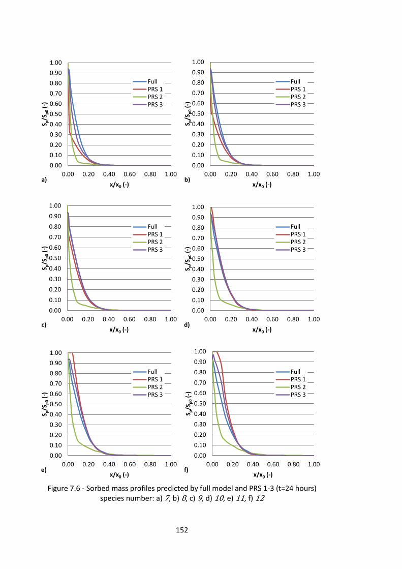
152
Figure 7.6 - Sorbed mass profiles predicted by full model and PRS 1-3 (t=24 hours)
species number: a) 7, b) 8, c) 9, d) 10, e) 11, f) 12
0.00
0.10
0.20
0.30
0.40
0.50
0.60
0.70
0.80
0.90
1.00
0.00 0.20 0.40 0.60 0.80 1.00
S p/S
p0 (
-)
x/x0 (-) a)
FullPRS 1PRS 2PRS 3
0.00
0.10
0.20
0.30
0.40
0.50
0.60
0.70
0.80
0.90
1.00
0.00 0.20 0.40 0.60 0.80 1.00
S p/S
p0 (
-)
x/x0 (-) b)
FullPRS 1PRS 2PRS 3
0.00
0.10
0.20
0.30
0.40
0.50
0.60
0.70
0.80
0.90
1.00
0.00 0.20 0.40 0.60 0.80 1.00
S p/S
p0
(-)
x/x0 (-) c)
FullPRS 1PRS 2PRS 3
0.00
0.10
0.20
0.30
0.40
0.50
0.60
0.70
0.80
0.90
1.00
0.00 0.20 0.40 0.60 0.80 1.00
S p/S
p0 (
-)
x/x0 (-) d)
FullPRS 1PRS 2PRS 3
0.00
0.10
0.20
0.30
0.40
0.50
0.60
0.70
0.80
0.90
1.00
0.00 0.20 0.40 0.60 0.80 1.00
S p/S
p0 (
-)
x/x0 (-) e)
FullPRS 1PRS 2PRS 3
0.00
0.10
0.20
0.30
0.40
0.50
0.60
0.70
0.80
0.90
1.00
0.00 0.20 0.40 0.60 0.80 1.00
S p/S
p0 (
-)
x/x0 (-) f)
FullPRS 1PRS 2PRS 3
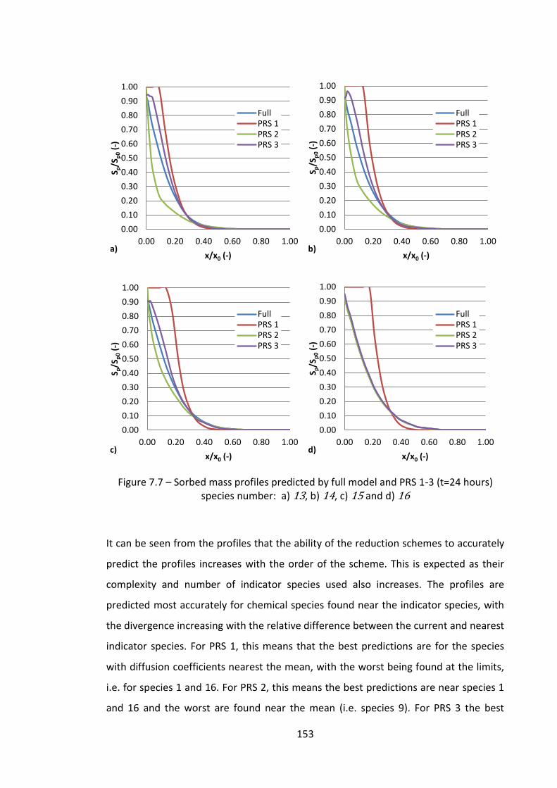
153
Figure 7.7 – Sorbed mass profiles predicted by full model and PRS 1-3 (t=24 hours) species number: a) 13, b) 14, c) 15 and d) 16
It can be seen from the profiles that the ability of the reduction schemes to accurately
predict the profiles increases with the order of the scheme. This is expected as their
complexity and number of indicator species used also increases. The profiles are
predicted most accurately for chemical species found near the indicator species, with
the divergence increasing with the relative difference between the current and nearest
indicator species. For PRS 1, this means that the best predictions are for the species
with diffusion coefficients nearest the mean, with the worst being found at the limits,
i.e. for species 1 and 16. For PRS 2, this means the best predictions are near species 1
and 16 and the worst are found near the mean (i.e. species 9). For PRS 3 the best
0.00
0.10
0.20
0.30
0.40
0.50
0.60
0.70
0.80
0.90
1.00
0.00 0.20 0.40 0.60 0.80 1.00
S p/S
p0 (
-)
x/x0 (-) a)
FullPRS 1PRS 2PRS 3
0.00
0.10
0.20
0.30
0.40
0.50
0.60
0.70
0.80
0.90
1.00
0.00 0.20 0.40 0.60 0.80 1.00
S p/S
p0 (
-)
x/x0 (-) b)
FullPRS 1PRS 2PRS 3
0.00
0.10
0.20
0.30
0.40
0.50
0.60
0.70
0.80
0.90
1.00
0.00 0.20 0.40 0.60 0.80 1.00
S p/S
p0
(-)
x/x0 (-) c)
FullPRS 1PRS 2PRS 3
0.00
0.10
0.20
0.30
0.40
0.50
0.60
0.70
0.80
0.90
1.00
0.00 0.20 0.40 0.60 0.80 1.00
S p/S
p0 (
-)
x/x0 (-) d)
FullPRS 1PRS 2PRS 3
154
predictions are found near species 1, 9, & 16, with the worst profile being found at
species 3, 4, 12 and 14.
7.2.1.1 Error and Correlation
In order to determine the accuracy of each reduction scheme, both the relative error
between the reduced and full models and the correlation between the profiles has
been investigated. The relative error is defined as:
(
)
(7.4)
The relative error plots for the concentration can be seen in Figure 7.8, whilst the
sorbed mass relative error can be seen in Figure 7.9.
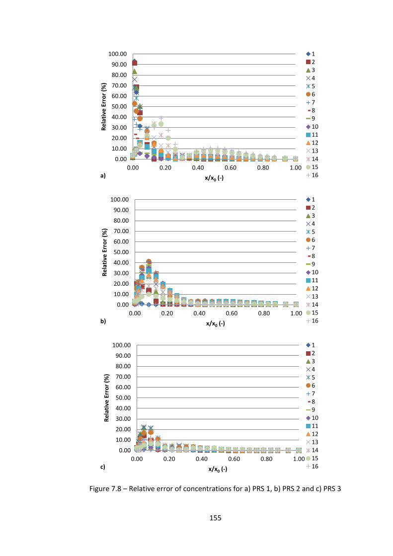
155
Figure 7.8 – Relative error of concentrations for a) PRS 1, b) PRS 2 and c) PRS 3
0.00
10.00
20.00
30.00
40.00
50.00
60.00
70.00
80.00
90.00
100.00
0.00 0.20 0.40 0.60 0.80 1.00
Re
lati
ve E
rro
r (%
)
x/x0 (-) a)
12345678910111213141516
0.00
10.00
20.00
30.00
40.00
50.00
60.00
70.00
80.00
90.00
100.00
0.00 0.20 0.40 0.60 0.80 1.00
Re
lati
ve E
rro
r (%
)
x/x0 (-) b)
12345678910111213141516
0.00
10.00
20.00
30.00
40.00
50.00
60.00
70.00
80.00
90.00
100.00
0.00 0.20 0.40 0.60 0.80 1.00
Re
lati
ve E
rro
r (%
)
x/x0 (-) c)
12345678910111213141516
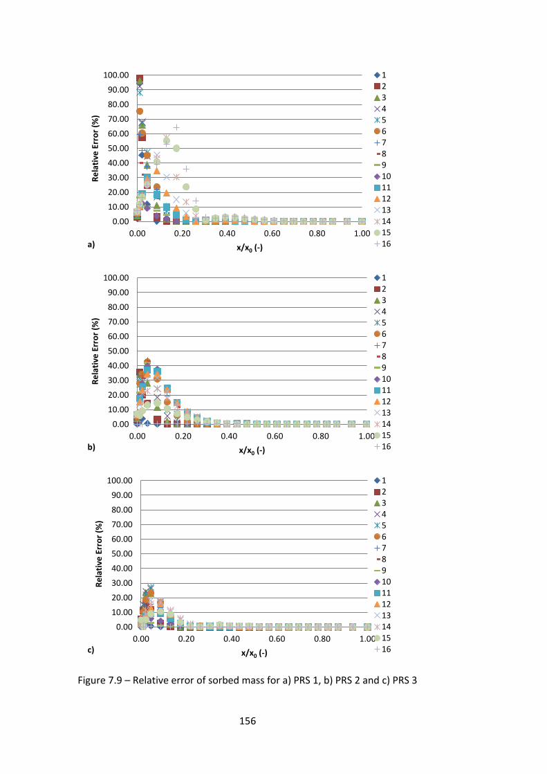
156
Figure 7.9 – Relative error of sorbed mass for a) PRS 1, b) PRS 2 and c) PRS 3
0.00
10.00
20.00
30.00
40.00
50.00
60.00
70.00
80.00
90.00
100.00
0.00 0.20 0.40 0.60 0.80 1.00
Re
lati
ve E
rro
r (%
)
x/x0 (-) a)
12345678910111213141516
0.00
10.00
20.00
30.00
40.00
50.00
60.00
70.00
80.00
90.00
100.00
0.00 0.20 0.40 0.60 0.80 1.00
Re
lati
ve E
rro
r (%
)
x/x0 (-) b)
12345678910111213141516
0.00
10.00
20.00
30.00
40.00
50.00
60.00
70.00
80.00
90.00
100.00
0.00 0.20 0.40 0.60 0.80 1.00
Re
lati
ve E
rro
r (%
)
x/x0 (-) c)
12345678910111213141516
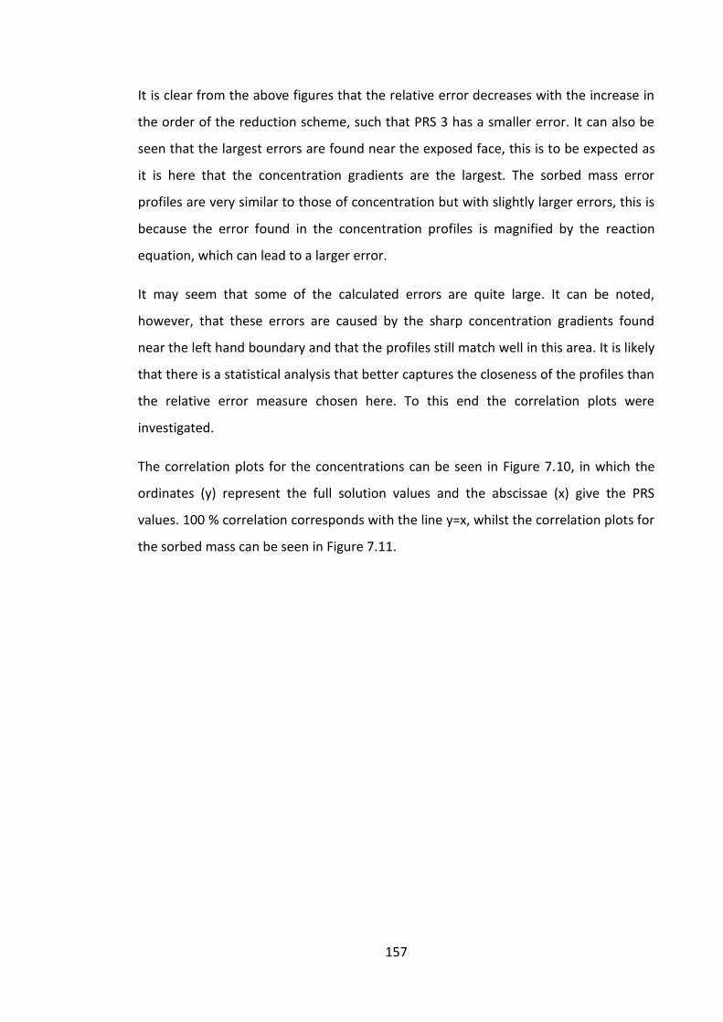
157
It is clear from the above figures that the relative error decreases with the increase in
the order of the reduction scheme, such that PRS 3 has a smaller error. It can also be
seen that the largest errors are found near the exposed face, this is to be expected as
it is here that the concentration gradients are the largest. The sorbed mass error
profiles are very similar to those of concentration but with slightly larger errors, this is
because the error found in the concentration profiles is magnified by the reaction
equation, which can lead to a larger error.
It may seem that some of the calculated errors are quite large. It can be noted,
however, that these errors are caused by the sharp concentration gradients found
near the left hand boundary and that the profiles still match well in this area. It is likely
that there is a statistical analysis that better captures the closeness of the profiles than
the relative error measure chosen here. To this end the correlation plots were
investigated.
The correlation plots for the concentrations can be seen in Figure 7.10, in which the
ordinates (y) represent the full solution values and the abscissae (x) give the PRS
values. 100 % correlation corresponds with the line y=x, whilst the correlation plots for
the sorbed mass can be seen in Figure 7.11.
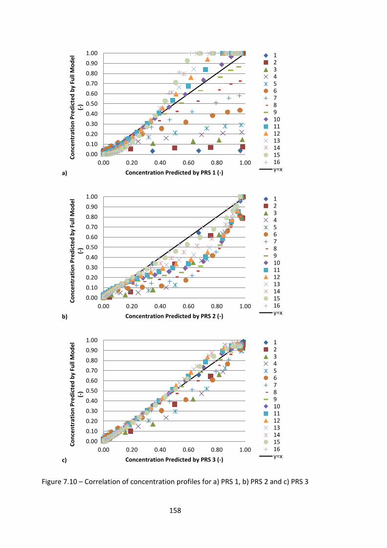
158
Figure 7.10 – Correlation of concentration profiles for a) PRS 1, b) PRS 2 and c) PRS 3
0.00
0.10
0.20
0.30
0.40
0.50
0.60
0.70
0.80
0.90
1.00
0.00 0.20 0.40 0.60 0.80 1.00
Co
nce
ntr
atio
n P
red
icte
d b
y Fu
ll M
od
el
(-)
Concentration Predicted by PRS 1 (-) a)
12345678910111213141516y=x
0.00
0.10
0.20
0.30
0.40
0.50
0.60
0.70
0.80
0.90
1.00
0.00 0.20 0.40 0.60 0.80 1.00
Co
nce
ntr
atio
n P
red
icte
d b
y Fu
ll M
od
el
(-)
Concentration Predicted by PRS 2 (-) b)
12345678910111213141516y=x
0.00
0.10
0.20
0.30
0.40
0.50
0.60
0.70
0.80
0.90
1.00
0.00 0.20 0.40 0.60 0.80 1.00
Co
nce
ntr
atio
n P
red
icte
d b
y Fu
ll M
od
el
(-)
Concentration Predicted by PRS 3 (-) c)
12345678910111213141516y=x
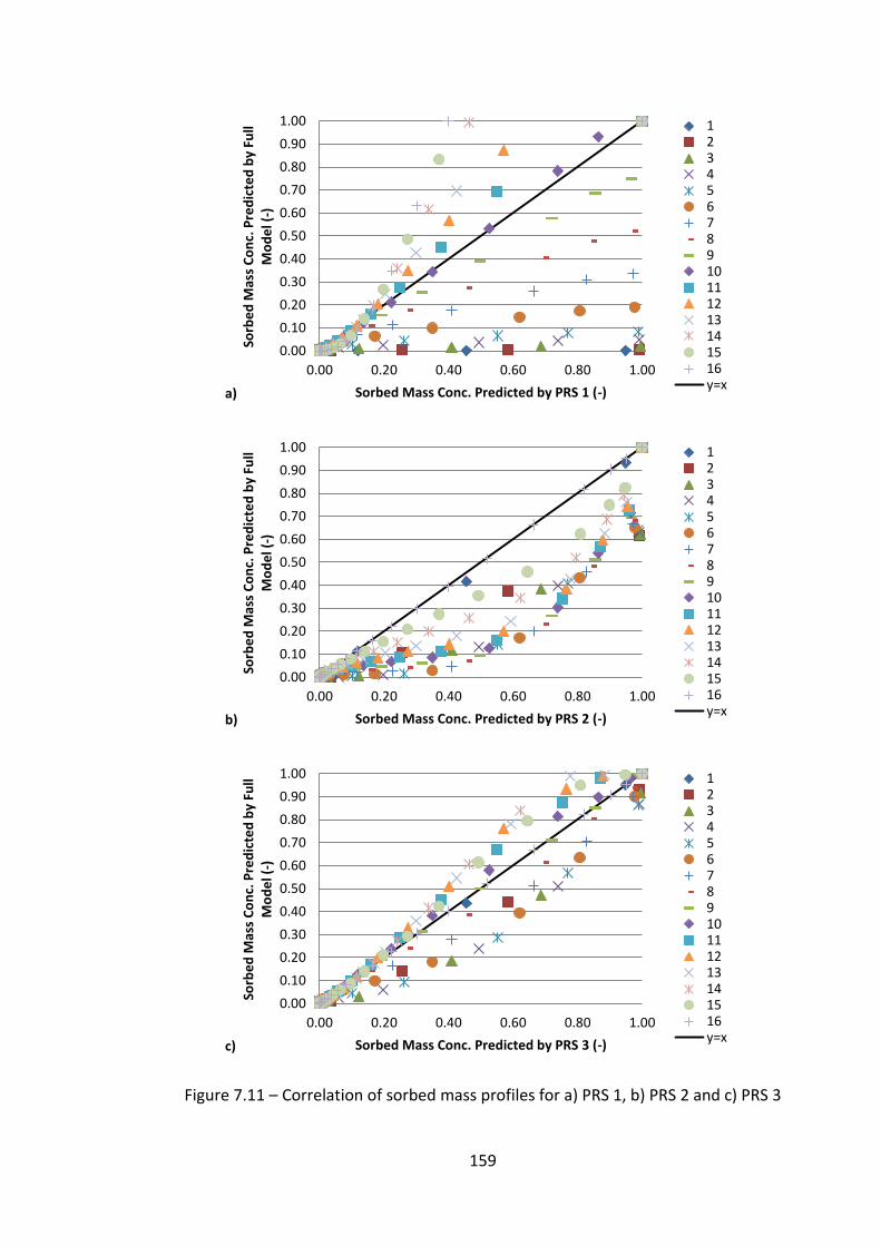
159
Figure 7.11 – Correlation of sorbed mass profiles for a) PRS 1, b) PRS 2 and c) PRS 3
0.00
0.10
0.20
0.30
0.40
0.50
0.60
0.70
0.80
0.90
1.00
0.00 0.20 0.40 0.60 0.80 1.00
Sorb
ed
Mas
s C
on
c. P
red
icte
d b
y Fu
ll M
od
el (
-)
Sorbed Mass Conc. Predicted by PRS 1 (-) a)
12345678910111213141516y=x
0.00
0.10
0.20
0.30
0.40
0.50
0.60
0.70
0.80
0.90
1.00
0.00 0.20 0.40 0.60 0.80 1.00
Sorb
ed
Mas
s C
on
c. P
red
icte
d b
y Fu
ll M
od
el (
-)
Sorbed Mass Conc. Predicted by PRS 2 (-) b)
12345678910111213141516y=x
0.00
0.10
0.20
0.30
0.40
0.50
0.60
0.70
0.80
0.90
1.00
0.00 0.20 0.40 0.60 0.80 1.00
Sorb
ed
Mas
s C
on
c. P
red
icte
d b
y Fu
ll M
od
el (
-)
Sorbed Mass Conc. Predicted by PRS 3 (-) c)
12345678910111213141516y=x
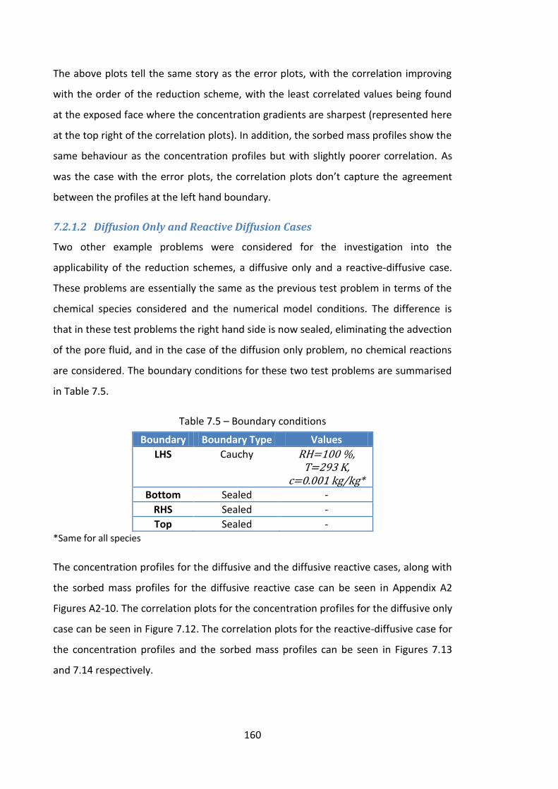
160
The above plots tell the same story as the error plots, with the correlation improving
with the order of the reduction scheme, with the least correlated values being found
at the exposed face where the concentration gradients are sharpest (represented here
at the top right of the correlation plots). In addition, the sorbed mass profiles show the
same behaviour as the concentration profiles but with slightly poorer correlation. As
was the case with the error plots, the correlation plots don’t capture the agreement
between the profiles at the left hand boundary.
7.2.1.2 Diffusion Only and Reactive Diffusion Cases
Two other example problems were considered for the investigation into the
applicability of the reduction schemes, a diffusive only and a reactive-diffusive case.
These problems are essentially the same as the previous test problem in terms of the
chemical species considered and the numerical model conditions. The difference is
that in these test problems the right hand side is now sealed, eliminating the advection
of the pore fluid, and in the case of the diffusion only problem, no chemical reactions
are considered. The boundary conditions for these two test problems are summarised
in Table 7.5.
Table 7.5 – Boundary conditions
Boundary Boundary Type Values
LHS Cauchy RH=100 %, T=293 K,
c=0.001 kg/kg* Bottom Sealed -
RHS Sealed -
Top Sealed - *Same for all species
The concentration profiles for the diffusive and the diffusive reactive cases, along with
the sorbed mass profiles for the diffusive reactive case can be seen in Appendix A2
Figures A2-10. The correlation plots for the concentration profiles for the diffusive only
case can be seen in Figure 7.12. The correlation plots for the reactive-diffusive case for
the concentration profiles and the sorbed mass profiles can be seen in Figures 7.13
and 7.14 respectively.
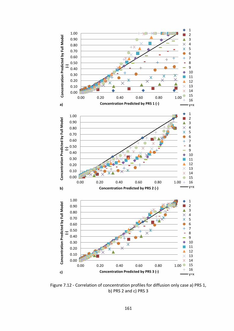
161
Figure 7.12 - Correlation of concentration profiles for diffusion only case a) PRS 1, b) PRS 2 and c) PRS 3
0.00
0.10
0.20
0.30
0.40
0.50
0.60
0.70
0.80
0.90
1.00
0.00 0.20 0.40 0.60 0.80 1.00Co
nce
ntr
atio
n P
red
icte
d b
y Fu
ll M
od
el
(-)
Concentration Predicted by PRS 1 (-) a)
12345678910111213141516y=x
0.00
0.10
0.20
0.30
0.40
0.50
0.60
0.70
0.80
0.90
1.00
0.00 0.20 0.40 0.60 0.80 1.00
Co
nce
ntr
atio
n P
red
icte
d b
y Fu
ll M
od
el
(-)
Concentration Predicted by PRS 2 (-) b)
12345678910111213141516y=x
0.00
0.10
0.20
0.30
0.40
0.50
0.60
0.70
0.80
0.90
1.00
0.00 0.20 0.40 0.60 0.80 1.00
Co
nce
ntr
atio
n P
red
icte
d b
y Fu
ll M
od
el
(-)
Concentration Predicted by PRS 3 (-) c)
12345678910111213141516y=x
162
Figure 7.13 - Correlation of concentration profiles for diffusive reactive case a) PRS 1, b) PRS 2 and c) PRS 3
0.00
0.10
0.20
0.30
0.40
0.50
0.60
0.70
0.80
0.90
1.00
0.00 0.20 0.40 0.60 0.80 1.00
Co
nce
ntr
atio
n P
red
icte
d b
y Fu
ll M
od
el
(-)
Concentration Predicted by PRS 1 (-) a)
12345678910111213141516y=x
0.00
0.10
0.20
0.30
0.40
0.50
0.60
0.70
0.80
0.90
1.00
0.00 0.20 0.40 0.60 0.80 1.00
Co
nce
ntr
atio
n P
red
icte
d b
y Fu
ll M
od
el
(-)
Concentration Predicted by PRS 2 (-) b)
12345678910111213141516y=x
0.00
0.10
0.20
0.30
0.40
0.50
0.60
0.70
0.80
0.90
1.00
0.00 0.20 0.40 0.60 0.80 1.00
Co
nce
ntr
atio
n P
red
icte
d b
y Fu
ll M
od
el
(-)
Concentration Predicted by PRS 3 (-) c)
12345678910111213141516y=x
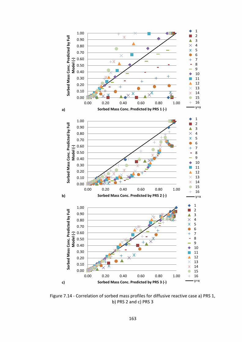
163
Figure 7.14 - Correlation of sorbed mass profiles for diffusive reactive case a) PRS 1, b) PRS 2 and c) PRS 3
0.00
0.10
0.20
0.30
0.40
0.50
0.60
0.70
0.80
0.90
1.00
0.00 0.20 0.40 0.60 0.80 1.00
Sorb
ed
Mas
s C
on
c. P
red
icte
d b
y Fu
ll M
od
el (
-)
Sorbed Mass Conc. Predicted by PRS 1 (-) a)
12345678910111213141516y=x
0.00
0.10
0.20
0.30
0.40
0.50
0.60
0.70
0.80
0.90
1.00
0.00 0.20 0.40 0.60 0.80 1.00
Sorb
ed
Mas
s C
on
c. P
red
icte
d b
y Fu
ll M
od
el (
-)
Sorbed Mass Conc. Predicted by PRS 2 (-) b)
12345678910111213141516y=x
0.00
0.10
0.20
0.30
0.40
0.50
0.60
0.70
0.80
0.90
1.00
0.00 0.20 0.40 0.60 0.80 1.00
Sorb
ed
Mas
s C
on
c. P
red
icte
d b
y Fu
ll M
od
el (
-)
Sorbed Mass Conc. Predicted by PRS 3 (-) c)
12345678910111213141516y=x
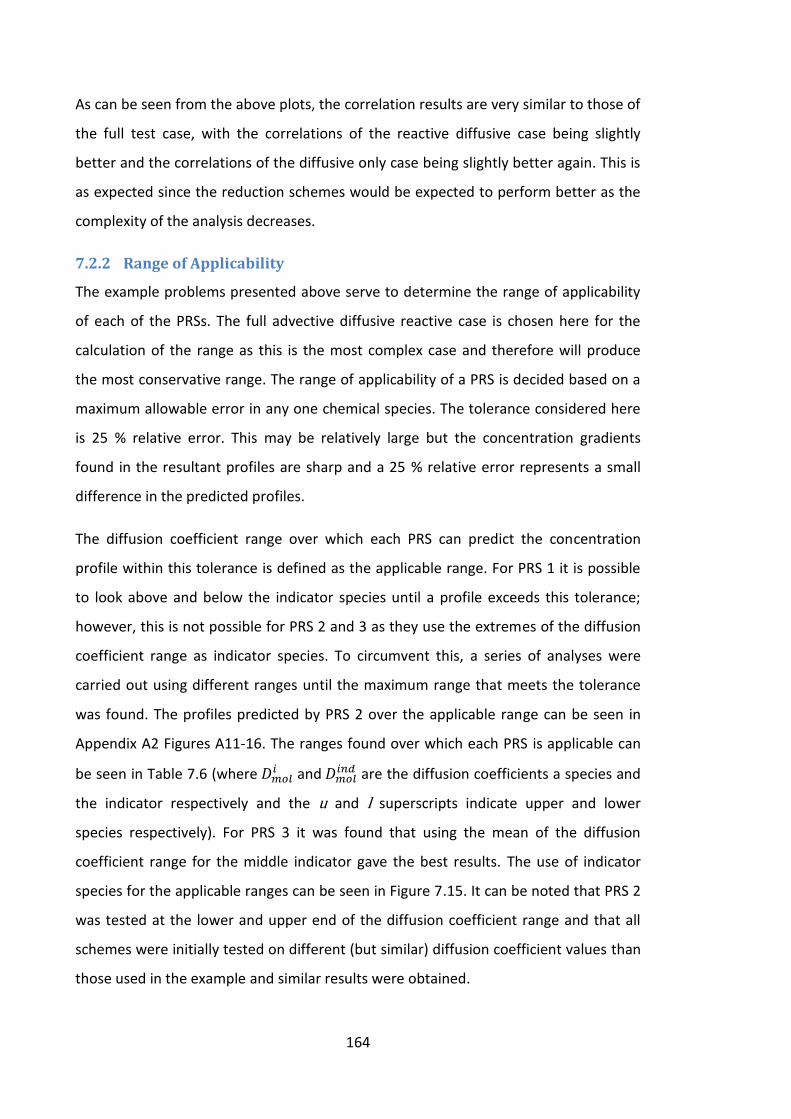
164
As can be seen from the above plots, the correlation results are very similar to those of
the full test case, with the correlations of the reactive diffusive case being slightly
better and the correlations of the diffusive only case being slightly better again. This is
as expected since the reduction schemes would be expected to perform better as the
complexity of the analysis decreases.
7.2.2 Range of Applicability
The example problems presented above serve to determine the range of applicability
of each of the PRSs. The full advective diffusive reactive case is chosen here for the
calculation of the range as this is the most complex case and therefore will produce
the most conservative range. The range of applicability of a PRS is decided based on a
maximum allowable error in any one chemical species. The tolerance considered here
is 25 % relative error. This may be relatively large but the concentration gradients
found in the resultant profiles are sharp and a 25 % relative error represents a small
difference in the predicted profiles.
The diffusion coefficient range over which each PRS can predict the concentration
profile within this tolerance is defined as the applicable range. For PRS 1 it is possible
to look above and below the indicator species until a profile exceeds this tolerance;
however, this is not possible for PRS 2 and 3 as they use the extremes of the diffusion
coefficient range as indicator species. To circumvent this, a series of analyses were
carried out using different ranges until the maximum range that meets the tolerance
was found. The profiles predicted by PRS 2 over the applicable range can be seen in
Appendix A2 Figures A11-16. The ranges found over which each PRS is applicable can
be seen in Table 7.6 (where and
are the diffusion coefficients a species and
the indicator respectively and the u and l superscripts indicate upper and lower
species respectively). For PRS 3 it was found that using the mean of the diffusion
coefficient range for the middle indicator gave the best results. The use of indicator
species for the applicable ranges can be seen in Figure 7.15. It can be noted that PRS 2
was tested at the lower and upper end of the diffusion coefficient range and that all
schemes were initially tested on different (but similar) diffusion coefficient values than
those used in the example and similar results were obtained.
165
Table 7.6 - Applicable ranges for PRSs
PRS 1 2 3
Diffusion Coefficient Range
0.8 <
<1.6
, <16 ,
, <64 ,
Figure 7.15 – Use of indicator species a) PRS 1, b) PRS 2 and c) PRS 3
7.2.3 Mass Balance
The PRSs have been shown to perform well in accurately predicting the chemical
behaviour of various systems; one concern, however, is that as the governing balance
equations are only solved for the indicator species and therefore mass balance may
not be maintained for the remaining species. For this reason, the mass balance error of
the PRSs has been investigated through the example problem. The total mass balance
0.0
0.1
0.2
0.3
0.4
0.5
0.6
0.7
0.8
0.9
1.0
0 0.5 1
c/c o
(-)
x/x0 (-) a)
D,ind
0.8*D,ind
1.6*D,ind
0
0.1
0.2
0.3
0.4
0.5
0.6
0.7
0.8
0.9
1
0 0.5 1
c/c o
(-)
x/x0 (-) b)
D,ind,l
16*D,ind,l
D
0
0.1
0.2
0.3
0.4
0.5
0.6
0.7
0.8
0.9
1
0 0.5 1
c/c o
(-)
x/x0 (-) c)
D,ind,lD,ind,m64*D,ind,lD
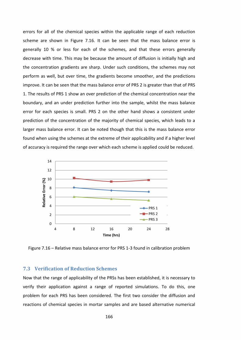
166
errors for all of the chemical species within the applicable range of each reduction
scheme are shown in Figure 7.16. It can be seen that the mass balance error is
generally 10 % or less for each of the schemes, and that these errors generally
decrease with time. This may be because the amount of diffusion is initially high and
the concentration gradients are sharp. Under such conditions, the schemes may not
perform as well, but over time, the gradients become smoother, and the predictions
improve. It can be seen that the mass balance error of PRS 2 is greater than that of PRS
1. The results of PRS 1 show an over prediction of the chemical concentration near the
boundary, and an under prediction further into the sample, whilst the mass balance
error for each species is small. PRS 2 on the other hand shows a consistent under
prediction of the concentration of the majority of chemical species, which leads to a
larger mass balance error. It can be noted though that this is the mass balance error
found when using the schemes at the extreme of their applicability and if a higher level
of accuracy is required the range over which each scheme is applied could be reduced.
Figure 7.16 – Relative mass balance error for PRS 1-3 found in calibration problem
7.3 Verification of Reduction Schemes
Now that the range of applicability of the PRSs has been established, it is necessary to
verify their application against a range of reported simulations. To do this, one
problem for each PRS has been considered. The first two consider the diffusion and
reactions of chemical species in mortar samples and are based alternative numerical
0
2
4
6
8
10
12
14
4 8 12 16 20 24 28
Re
lati
ve E
rro
r (%
)
Time (hrs)
PRS 1
PRS 2
PRS 3
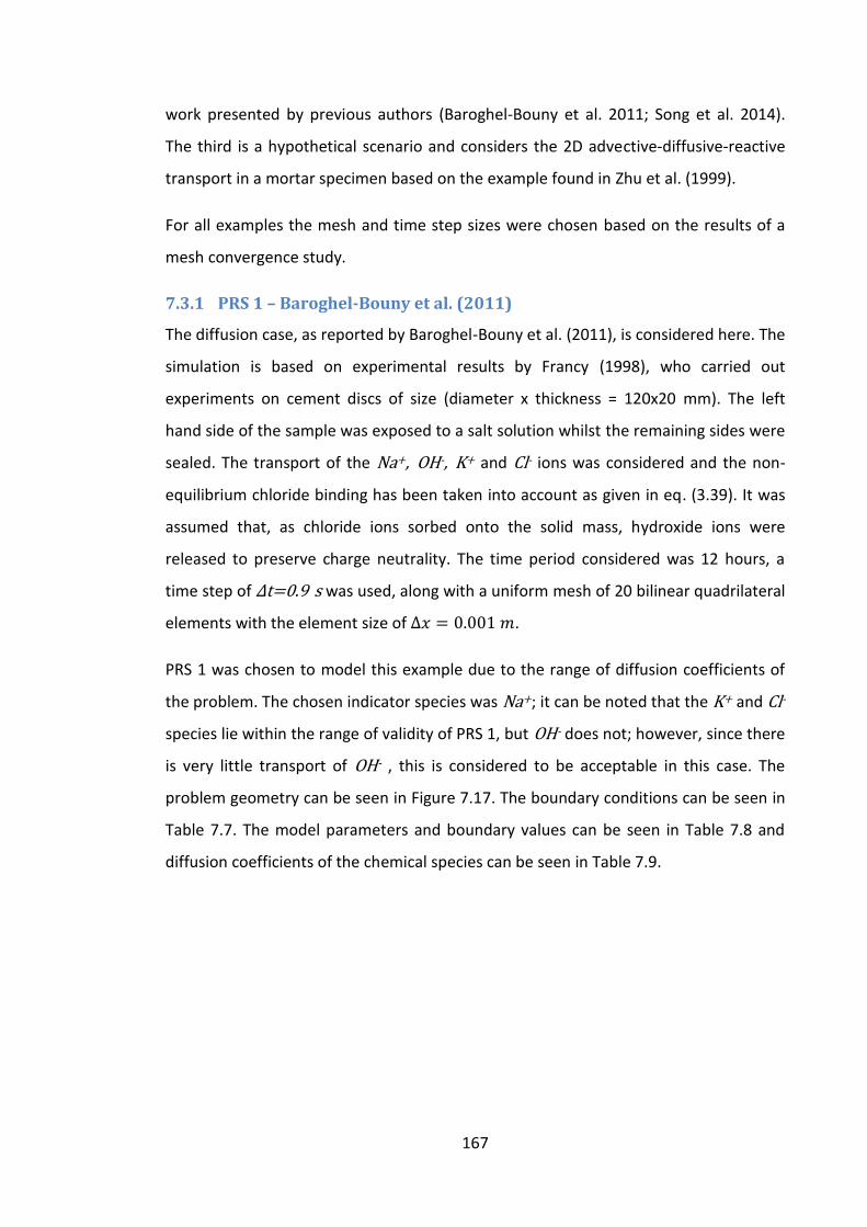
167
work presented by previous authors (Baroghel-Bouny et al. 2011; Song et al. 2014).
The third is a hypothetical scenario and considers the 2D advective-diffusive-reactive
transport in a mortar specimen based on the example found in Zhu et al. (1999).
For all examples the mesh and time step sizes were chosen based on the results of a
mesh convergence study.
7.3.1 PRS 1 – Baroghel-Bouny et al. (2011)
The diffusion case, as reported by Baroghel-Bouny et al. (2011), is considered here. The
simulation is based on experimental results by Francy (1998), who carried out
experiments on cement discs of size (diameter x thickness = 120x20 mm). The left
hand side of the sample was exposed to a salt solution whilst the remaining sides were
sealed. The transport of the Na+, OH-, K+ and Cl- ions was considered and the non-
equilibrium chloride binding has been taken into account as given in eq. (3.39). It was
assumed that, as chloride ions sorbed onto the solid mass, hydroxide ions were
released to preserve charge neutrality. The time period considered was 12 hours, a
time step of t=0.9 s was used, along with a uniform mesh of 20 bilinear quadrilateral
elements with the element size of .
PRS 1 was chosen to model this example due to the range of diffusion coefficients of
the problem. The chosen indicator species was Na+; it can be noted that the K+ and Cl-
species lie within the range of validity of PRS 1, but OH- does not; however, since there
is very little transport of OH- , this is considered to be acceptable in this case. The
problem geometry can be seen in Figure 7.17. The boundary conditions can be seen in
Table 7.7. The model parameters and boundary values can be seen in Table 7.8 and
diffusion coefficients of the chemical species can be seen in Table 7.9.
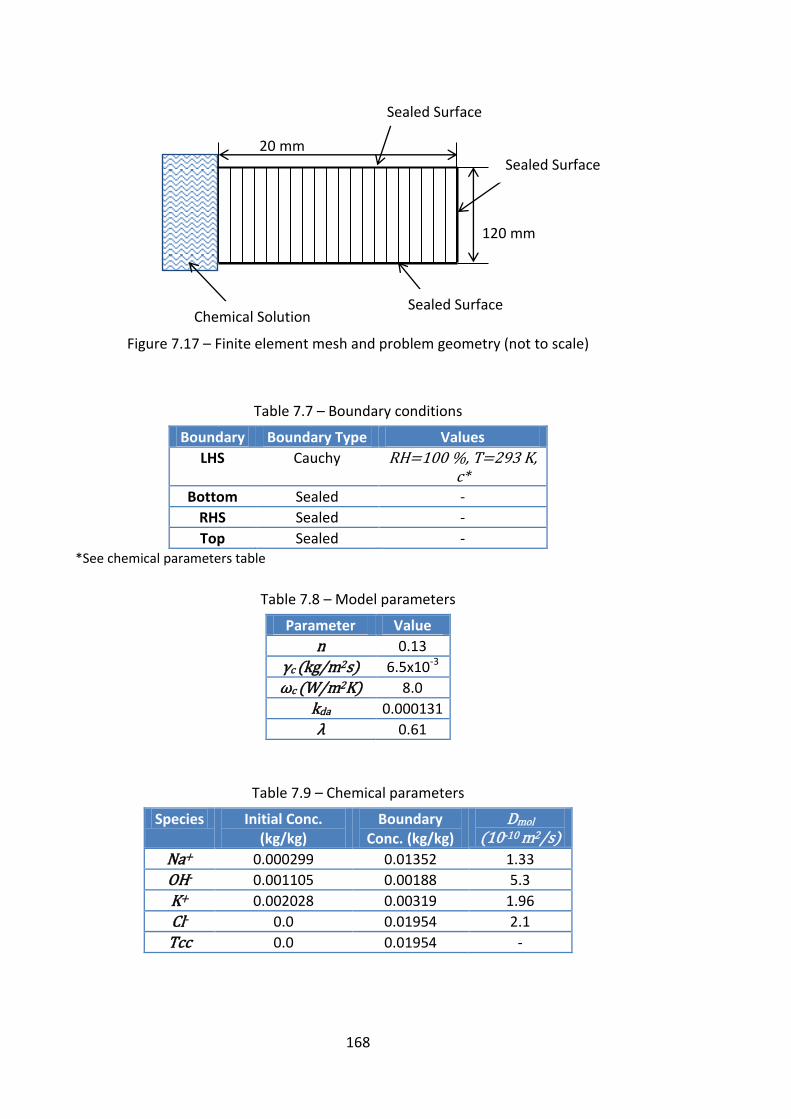
168
Figure 7.17 – Finite element mesh and problem geometry (not to scale)
Table 7.7 – Boundary conditions
Boundary Boundary Type Values
LHS Cauchy RH=100 %, T=293 K, c*
Bottom Sealed -
RHS Sealed -
Top Sealed - *See chemical parameters table
Table 7.8 – Model parameters
Parameter Value
n 0.13
γc (kg/m2s) 6.5x10⁻³
ωc (W/m2K) 8.0
kda 0.000131
λ 0.61
Table 7.9 – Chemical parameters
Species Initial Conc. (kg/kg)
Boundary Conc. (kg/kg)
Dmol
(10-10 m2/s)
Na+ 0.000299 0.01352 1.33
OH- 0.001105 0.00188 5.3
K+ 0.002028 0.00319 1.96
Cl- 0.0 0.01954 2.1
Tcc 0.0 0.01954 -
20 mm
120 mm
Chemical Solution Sealed Surface
Sealed Surface
Sealed Surface
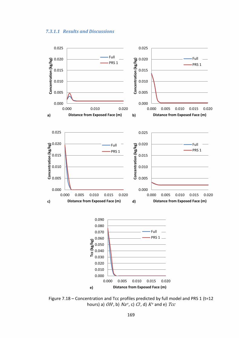
169
7.3.1.1 Results and Discussions
Figure 7.18 – Concentration and Tcc profiles predicted by full model and PRS 1 (t=12
hours) a) OH-, b) Na+, c) Cl-, d) K+ and e) Tcc
0.000
0.005
0.010
0.015
0.020
0.025
0.000 0.010 0.020
Co
nce
ntr
atio
n (
kg/k
g)
Distance from Exposed Face (m) a)
Full
PRS 1
0.000
0.005
0.010
0.015
0.020
0.025
0.000 0.005 0.010 0.015 0.020
Co
nce
ntr
atio
n (
kg/k
g)
Distance from Exposed Face (m) b)
Full
PRS 1
0.000
0.005
0.010
0.015
0.020
0.025
0.000 0.005 0.010 0.015 0.020
Co
nce
ntr
atio
n (
kg/k
g)
Distance from Exposed Face (m) c)
Full
PRS 1
0.000
0.005
0.010
0.015
0.020
0.025
0.000 0.005 0.010 0.015 0.020
Co
nce
ntr
atio
n (
kg/k
g)
Distance from Exposed Face (m) d)
Full
PRS 1
0.000
0.010
0.020
0.030
0.040
0.050
0.060
0.070
0.080
0.090
0.000 0.005 0.010 0.015 0.020
Tcc
(kg/
kg)
Distance from Exposed Face (m) e)
Full
PRS 1
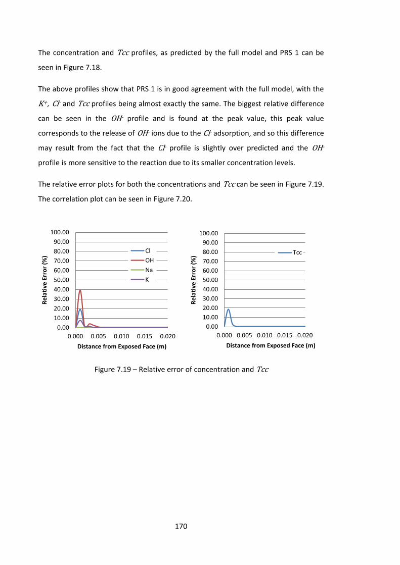
170
The concentration and Tcc profiles, as predicted by the full model and PRS 1 can be
seen in Figure 7.18.
The above profiles show that PRS 1 is in good agreement with the full model, with the
K+, Cl- and Tcc profiles being almost exactly the same. The biggest relative difference
can be seen in the OH- profile and is found at the peak value, this peak value
corresponds to the release of OH- ions due to the Cl- adsorption, and so this difference
may result from the fact that the Cl- profile is slightly over predicted and the OH-
profile is more sensitive to the reaction due to its smaller concentration levels.
The relative error plots for both the concentrations and Tcc can be seen in Figure 7.19.
The correlation plot can be seen in Figure 7.20.
Figure 7.19 – Relative error of concentration and Tcc
0.00
10.00
20.00
30.00
40.00
50.00
60.00
70.00
80.00
90.00
100.00
0.000 0.005 0.010 0.015 0.020
Re
lati
ve E
rro
r (%
)
Distance from Exposed Face (m)
Cl
OH
Na
K
0.00
10.00
20.00
30.00
40.00
50.00
60.00
70.00
80.00
90.00
100.00
0.000 0.005 0.010 0.015 0.020
Re
lati
ve E
rro
r (%
)
Distance from Exposed Face (m)
Tcc
171
Figure 7.20 – Correlation plot of concentrations and Tcc
The above plots are in agreement with the profiles showing the largest error, and least
correlation, for the OH- profile.
A mass balance check was also carried out, from which the results are given in in Table
7.10. It can be seen from this table that the maximum mass balance error is 17 % and
is found in the Cl- profile not the OH- profile which showed the largest relative error.
This is due to the over prediction of the penetration of the Cl- ions into the beam.
Table 7.10 – Relative mass balance error induced by PRS 1 (%)
Na+ Cl- OH- K+ Tcc
0.13 17.02 4.22 0.25 15.82
7.3.2 PRS 2 – Song et al. (2014)
The diffusion experiments and accompanying numerical simulations presented by Song
et al. (2014) are considered here. In their work, a concrete slab was cured for 90 days
and subsequently a set of 100x50 mm (diameter x thickness) cylindrical core of; the
sides and bottom were sealed before the remaining surface was exposed to a salt
solution for 6 months.
The boundary concentrations can be can be found in in Table 7.13 along with the
diffusion coefficients and the Des factors, which account for electrostatic double-layer
0.00
0.10
0.20
0.30
0.40
0.50
0.60
0.70
0.80
0.90
1.00
0.00 0.10 0.20 0.30 0.40 0.50 0.60 0.70 0.80 0.90 1.00Co
nce
ntr
atio
n a
nd
Tcc
Pre
dic
ted
by
Full
Mo
de
l (-)
Concentration and Tcc Predicted by PRS 1 (-)
Cl
OH
Na
K
Tcc
y=x
172
effects (Song et al. 2014). The sample was assumed to be initially saturated, with no
solid masses present and the time period considered was 2 months. The time step size
chosen was and a mesh of 52 bilinear quadrilateral elements was used
with an element size of . The problem geometry can be seen in Figure
7.21. The boundary conditions can be seen in Table 7.11. Table 7.12 shows the model
parameters of the specimen. PRS 2 was chosen to model this example as the diffusion
coefficient range is less than 6 ( , <16
, ), the OH- and K+ species were chosen
as the indicator species in this case as they are the species with the highest and lowest
diffusion coefficients respectively (following multiplication by the Des factors). The non-
equilibrium Freundlich type isotherm describes the reactions, which were given in eqs.
(6.5-6.9 & 6.12).
Figure 7.21 – Finite element mesh and problem geometry (not to scale)
Table 7.11 – Boundary conditions
Boundary Boundary Type Values
LHS Cauchy RH=100 %, T=293 K, c*
Bottom Sealed -
RHS Sealed -
Top Sealed - *See chemical parameters table
50 mm
100 mm
Chemical Solution
Sealed Surface
Sealed Surface
Sealed Surface
173
Table 7.12 – Model parameters
Parameter Value
n 0.13
γc (kg/m2s) 1e-4
ωc (W/m2K) 8.0
Table 7.13 – Chemical parameters
Species Initial Conc.
(kg/kg)
Bound. Conc.
(kg/kg)
Dmol
(10-9 m2/s) Des Eq. ka (10-8) kd (10-8) λ
Na+ 0.001978 0.0 1.33 0.25 r1 12.0 18.0 0.35
OH- 0.004573 0.0 5.3 0.25 r2 144.0 24.0 0.35
K+ 0.007215 0.0 1.96 0.0875 r3 1375.0 330.0 0.35
Cl- 0.0 0.01775 2.1 0.25 r4 6.42 1.275 0.2
SO42- 0.000192 0.0 1.07 1.0 r5 5.4 0.75 0.2
Ca2+ 0.00004 0.01 0.79 0.4 r6 1000.00 1200.0 0.35
7.3.2.1 Results and Discussions
The concentration profiles as predicted by the full model and PRS 2 can be seen in
Figure 7.22, whilst the solid mass profiles can be seen in Figure 7.23.
174
Figure 7.22 – Concentration profiles predicted by full model and PRS 2 (t=2 months) a) Na+, b) K+, c) Ca2+, d) Cl-, e) OH- and f) SO42-
0.0000
0.0005
0.0010
0.0015
0.0020
0.0025
0.00 0.02 0.04
Co
nce
ntr
atio
n (
kg/k
g)
Distance from Exposed Face (m) a)
Full
PRS 20.000
0.001
0.002
0.003
0.004
0.005
0.006
0.007
0.008
0.00 0.02 0.04
Co
nce
ntr
atio
n (
kg/k
g)
Distance from Exposed Face (m) b)
Full
PRS 2
0.000
0.002
0.004
0.006
0.008
0.010
0.012
0.00 0.02 0.04
Co
nce
ntr
atio
n (
kg/k
g)
Distance from Exposed Face (m) c)
Full
PRS 2
0.000
0.002
0.004
0.006
0.008
0.010
0.012
0.014
0.016
0.018
0.020
0.00 0.02 0.04
Co
nce
ntr
atio
n (
kg/k
g)
Distance from Exposed Face (m) d)
Full
PRS 2
0.0000
0.0005
0.0010
0.0015
0.0020
0.0025
0.0030
0.0035
0.0040
0.0045
0.0050
0.00 0.02 0.04
Co
nce
ntr
atio
n (
kg/k
g)
Distance from Exposed Face (m) e)
Full
PRS 2
0.00000
0.00005
0.00010
0.00015
0.00020
0.00025
0.00 0.02 0.04
Co
nce
ntr
atio
n (
kg/k
g)
Distance from Exposed Face (m) f)
Full
PRS 2
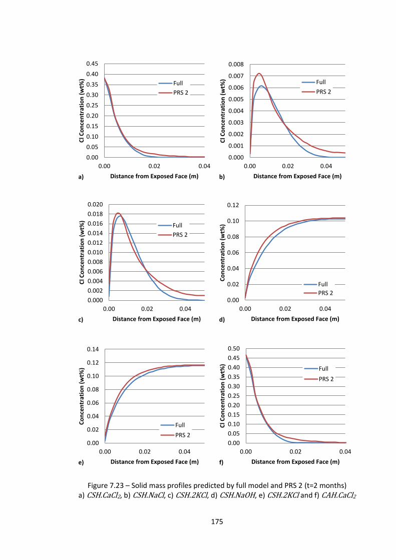
175
Figure 7.23 – Solid mass profiles predicted by full model and PRS 2 (t=2 months) a) CSH.CaCl2, b) CSH.NaCl, c) CSH.2KCl, d) CSH.NaOH, e) CSH.2KCl and f) CAH.CaCl2
0.00
0.05
0.10
0.15
0.20
0.25
0.30
0.35
0.40
0.45
0.00 0.02 0.04
Cl C
on
cen
trat
ion
(w
t%)
Distance from Exposed Face (m) a)
Full
PRS 2
0.000
0.001
0.002
0.003
0.004
0.005
0.006
0.007
0.008
0.00 0.02 0.04
Cl C
on
cen
trat
ion
(w
t%)
Distance from Exposed Face (m) b)
Full
PRS 2
0.000
0.002
0.004
0.006
0.008
0.010
0.012
0.014
0.016
0.018
0.020
0.00 0.02 0.04
Cl C
on
cen
trat
ion
(w
t%)
Distance from Exposed Face (m) c)
Full
PRS 2
0.00
0.02
0.04
0.06
0.08
0.10
0.12
0.00 0.02 0.04
Co
nce
ntr
atio
n (
wt%
)
Distance from Exposed Face (m) d)
Full
PRS 2
0.00
0.02
0.04
0.06
0.08
0.10
0.12
0.14
0.00 0.02 0.04
Co
nce
ntr
atio
n (
wt%
)
Distance from Exposed Face (m) e)
Full
PRS 20.00
0.05
0.10
0.15
0.20
0.25
0.30
0.35
0.40
0.45
0.50
0.00 0.02 0.04
Cl C
on
cen
trat
ion
(w
t%)
Distance from Exposed Face (m) f)
Full
PRS 2
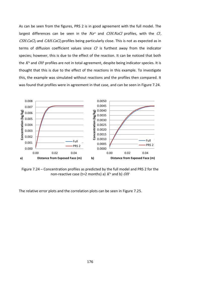
176
As can be seen from the figures, PRS 2 is in good agreement with the full model. The
largest differences can be seen in the Na+ and CSH.NaCl profiles, with the Cl-,
CSH.CaCl2 and CAH.CaCl2 profiles being particularly close. This is not as expected as in
terms of diffusion coefficient values since Cl- is furthest away from the indicator
species; however, this is due to the effect of the reaction. It can be noticed that both
the K+ and OH- profiles are not in total agreement, despite being indicator species. It is
thought that this is due to the effect of the reactions in this example. To investigate
this, the example was simulated without reactions and the profiles then compared. It
was found that profiles were in agreement in that case, and can be seen in Figure 7.24.
Figure 7.24 – Concentration profiles as predicted by the full model and PRS 2 for the non-reactive case (t=2 months) a) K+ and b) OH-
The relative error plots and the correlation plots can be seen in Figure 7.25.
0.000
0.001
0.002
0.003
0.004
0.005
0.006
0.007
0.008
0.00 0.02 0.04
Co
nce
ntr
atio
n (
kg/k
g)
Distance from Exposed Face (m) a)
Full
PRS 20.0000
0.0005
0.0010
0.0015
0.0020
0.0025
0.0030
0.0035
0.0040
0.0045
0.0050
0.00 0.02 0.04
Co
nce
ntr
atio
n (
kg/k
g)
Distance from Exposed Face (m) b)
Full
PRS 2
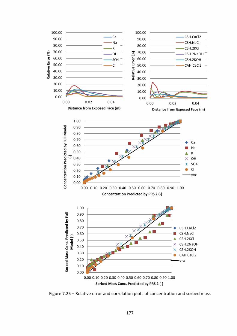
177
Figure 7.25 – Relative error and correlation plots of concentration and sorbed mass
0.00
10.00
20.00
30.00
40.00
50.00
60.00
70.00
80.00
90.00
100.00
0.00 0.02 0.04
Re
lati
ve E
rro
r (%
)
Distance from Exposed Face (m)
Ca
Na
K
OH
SO4
Cl
0.00
10.00
20.00
30.00
40.00
50.00
60.00
70.00
80.00
90.00
100.00
0.00 0.02 0.04
Re
lati
ve E
rro
r (%
)
Distance from Exposed Face (m)
CSH.CaCl2
CSH.NaCl
CSH.2KCl
CSH.2NaOH
CSH.2KOH
CAH.CaCl2
0.00
0.10
0.20
0.30
0.40
0.50
0.60
0.70
0.80
0.90
1.00
0.00 0.10 0.20 0.30 0.40 0.50 0.60 0.70 0.80 0.90 1.00Co
nce
ntr
atio
n P
red
icte
d b
y Fu
ll M
od
el
(-)
Concentration Predicted by PRS 2 (-)
Ca
Na
K
OH
SO4
Cl
y=x
0.00
0.10
0.20
0.30
0.40
0.50
0.60
0.70
0.80
0.90
1.00
0.00 0.10 0.20 0.30 0.40 0.50 0.60 0.70 0.80 0.90 1.00
Sorb
ed
Mas
s C
on
c. P
red
icte
d b
y Fu
ll M
od
el (
-)
Sorbed Mass Conc. Predicted by PRS 2 (-)
CSH.CaCl2
CSH.NaCl
CSH.2KCl
CSH.2NaOH
CSH.2KOH
CAH.CaCl2
y=x
178
The above plots are in agreement with the profiles showing the largest error and least
correlation to be in the Na+ and CSH.NaCl profiles.
A mass balance check was also carried out, the results of which can be seen in Table
7.14. It can be seen that the largest error is in the Ca2+ profile with a value of 31.05 %,
this is in agreement with the profiles as the Ca2+ shows a constant over-prediction.
Table 7.14 - Relative mass balance error induced by PRS 2 (%)
Ca2+ Na+ K+ OH- SO42- Cl-
31.05 5.23 2.30 7.35 7.07 2.16
CSH.CaCl2 CSH.NaCl CSH.2KCl CSH.2NaOH CSH.2KOH CAH.CaCl2
13.54 19.12 12.19 4.91 4.07 14.21
7.3.3 PRS 3 – Hypothetical based on Zhu et al. (1999)
The final simulation is based on the work of Zhu et al. (1999). It involves the transport
of 10 chemical species, precipitation of 6 minerals and considers 1 immobile solid
species. This is a 2D problem with a point source for the chemical species (marked A in
Figure 7.26). The moisture transport was considered at a constant rate of V=5.8x10⁻⁶
mm/s in the x direction. The total domain size was 12.5x10 mm. The problem
geometry can be seen in Figure 7.26; due to the symmetry of the problem, it was only
necessary to model half of the domain. The boundary conditions are of zero flux on all
sides. It was assumed that the sample was initially saturated and the time period
considered was 10 hours. The time step size chosen was t=3.6 s and a mesh of 286
bilinear quadratic elements was used with an element size of . The
Freundlich type isotherm (eq. 3.39) describes the reactions, which were calculated
based on the non-equilibrium assumption. The reaction equations for the 6 solid
minerals considered are given as:
( ) [ ( ) ]
( ) ([ ][ ] ) (7.5)
[ ]
([ ][ ][ ] ) (7.6)
( ) [ ( ) ]
( ) ([ ] [ ][ ] [ ( )
] [ ] ) (7.7)
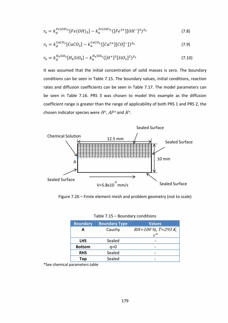
179
( ) [ ( ) ]
( ) ([ ][ ] ) (7.8)
[ ]
([ ][ ]) (7.9)
[ ]
([ ] [ ] ) (7.10)
It was assumed that the initial concentration of solid masses is zero. The boundary
conditions can be seen in Table 7.15. The boundary values, initial conditions, reaction
rates and diffusion coefficients can be seen in Table 7.17. The model parameters can
be seen in Table 7.16. PRS 3 was chosen to model this example as the diffusion
coefficient range is greater than the range of applicability of both PRS 1 and PRS 2, the
chosen indicator species were H+, Al3+ and K+.
Figure 7.26 – Finite element mesh and problem geometry (not to scale)
Table 7.15 – Boundary conditions
Boundary Boundary Type Values
A Cauchy RH=100 %, T=293 K, c*
LHS Sealed - Bottom q=0 -
RHS Sealed -
Top Sealed - *See chemical parameters table
12.5 mm
10 mm A
V=5.8x10⁻⁶
mm/s
Chemical Solution
Sealed Surface
Sealed Surface
Sealed Surface Sealed Surface
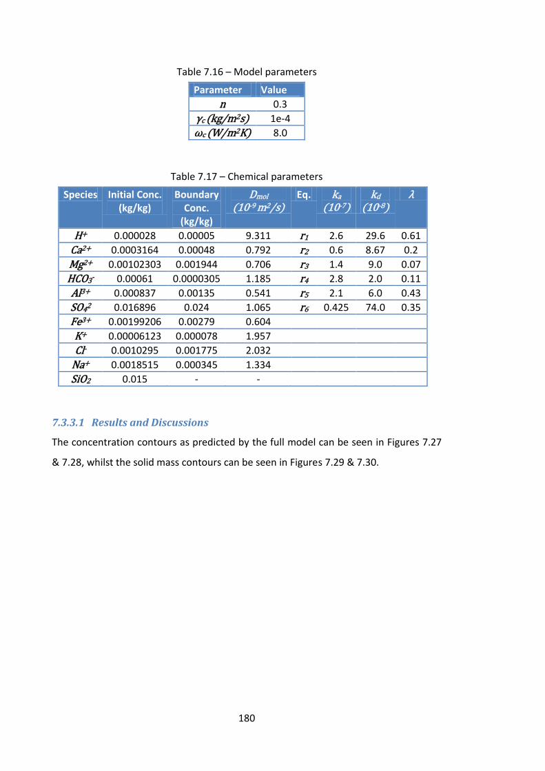
180
Table 7.16 – Model parameters
Parameter Value
n 0.3
γc (kg/m2s) 1e-4
ωc (W/m2K) 8.0
Table 7.17 – Chemical parameters
Species Initial Conc. (kg/kg)
Boundary Conc.
(kg/kg)
Dmol
(10-9 m2/s) Eq. ka
(10-7) kd
(10-8) λ
H+ 0.000028 0.00005 9.311 r1 2.6 29.6 0.61
Ca2+ 0.0003164 0.00048 0.792 r2 0.6 8.67 0.2
Mg2+ 0.00102303 0.001944 0.706 r3 1.4 9.0 0.07
HCO3- 0.00061 0.0000305 1.185 r4 2.8 2.0 0.11
Al3+ 0.000837 0.00135 0.541 r5 2.1 6.0 0.43
SO42 0.016896 0.024 1.065 r6 0.425 74.0 0.35
Fe3+ 0.00199206 0.00279 0.604
K+ 0.00006123 0.000078 1.957
Cl- 0.0010295 0.001775 2.032
Na+ 0.0018515 0.000345 1.334
SiO2 0.015 - -
7.3.3.1 Results and Discussions
The concentration contours as predicted by the full model can be seen in Figures 7.27
& 7.28, whilst the solid mass contours can be seen in Figures 7.29 & 7.30.
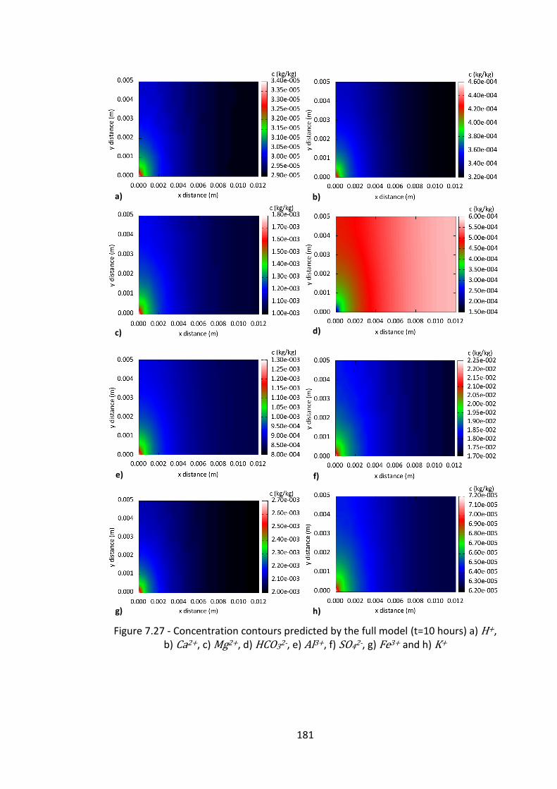
181
Figure 7.27 - Concentration contours predicted by the full model (t=10 hours) a) H+, b) Ca2+, c) Mg2+, d) HCO32-, e) Al3+, f) SO42-, g) Fe3+ and h) K+
a) b)
c) d)
e) f)
g) h)
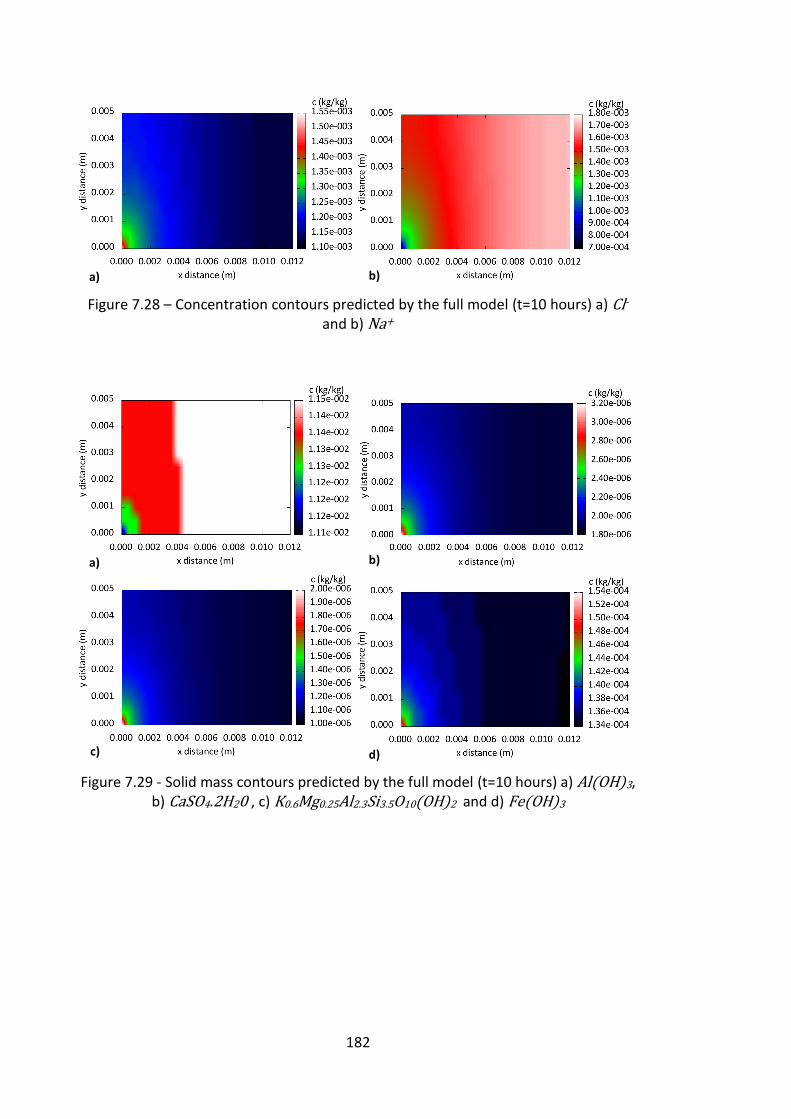
182
Figure 7.28 – Concentration contours predicted by the full model (t=10 hours) a) Cl- and b) Na+
Figure 7.29 - Solid mass contours predicted by the full model (t=10 hours) a) Al(OH)3, b) CaSO4.2H20 , c) K0.6Mg0.25Al2.3Si3.5O10(OH)2 and d) Fe(OH)3
a) b)
a) b)
c) d)
183
Figure 7.30 – Solid mass contours predicted by the full model (t=10 hours) a) CaCO3, b) H4SiO4 and c) SiO2
As can be seen from the contours, the behaviour is as expected with slightly higher
penetration of the solutes in the x direction as a result of the pore water velocity. Two
main types of behaviour are present in the chemical species; one relates to species for
which the boundary concentration is higher than the initial concentration, where the
chemical is transported into the domain, and the other for which concentrations are
lower, and the chemical diffuses out of the domain in a direction contrary to the
advective pore water flow.
The concentration profiles -as predicted by the full model and PRS 3- can be seen in
Figures 7.32 & 7.33, whilst the solid mass profiles can be seen in Figures 7.34 & 7.35.
These profiles are found by taking a cut along the x axis, line B-B seen in Figure 7.31.
The y profiles, obtained by taking a cut along line A-A, showed similar results and can
be seen in Appendix A2 Figures A19-22.
a) b)
c)
184
Figure 7.31 – Problem geometry and cut lines
Figure 7.32 - Concentration profiles (taken along cut line B-B) predicted by the full model and PRS 3 (t=10 hours) a) H+, b) Ca2+, c) Mg2+ and d) HCO32-
0.00E+00
5.00E-06
1.00E-05
1.50E-05
2.00E-05
2.50E-05
3.00E-05
3.50E-05
4.00E-05
0.000 0.005 0.010
Co
nce
ntr
atio
n (
kg/k
g)
Distance from Exposed Face (m) a)
Full
PRS 30.00E+00
5.00E-05
1.00E-04
1.50E-04
2.00E-04
2.50E-04
3.00E-04
3.50E-04
4.00E-04
4.50E-04
5.00E-04
0.000 0.005 0.010
Co
nce
ntr
atio
n (
kg/k
g)
Distance from Exposed Face (m) b)
Full
PRS 3
0.00E+00
2.00E-04
4.00E-04
6.00E-04
8.00E-04
1.00E-03
1.20E-03
1.40E-03
1.60E-03
1.80E-03
2.00E-03
0.000 0.005 0.010
Co
nce
ntr
atio
n (
kg/k
g)
Distance from Exposed Face (m) c)
Full
PRS 30.00E+00
1.00E-04
2.00E-04
3.00E-04
4.00E-04
5.00E-04
6.00E-04
7.00E-04
0.000 0.005 0.010
Co
nce
ntr
atio
n (
kg/k
g)
Distance from Exposed Face (m) d)
Full
PRS 3
12.5 mm
10 mm
A
A
B B
185
Figure 7.33 – Concentration profiles (taken along cut line B-B) predicted by the full model and PRS 3 (t=10 hours) a) Al3+, b) SO42-, c) Fe3+, d) K+, e) Cl- and f) Na+
0.00E+00
2.00E-04
4.00E-04
6.00E-04
8.00E-04
1.00E-03
1.20E-03
1.40E-03
0.000 0.005 0.010
Co
nce
ntr
atio
n (
kg/k
g)
Distance from Exposed Face (m) a)
Full
PRS 30.00E+00
5.00E-03
1.00E-02
1.50E-02
2.00E-02
2.50E-02
0.000 0.005 0.010
Co
nce
ntr
atio
n (
kg/k
g)
Distance from Exposed Face (m) b)
Full
PRS 3
0.00E+00
5.00E-04
1.00E-03
1.50E-03
2.00E-03
2.50E-03
3.00E-03
0.000 0.005 0.010
Co
nce
ntr
atio
n (
kg/k
g)
Distance from Exposed Face (m) c)
Full
PRS 30.00E+00
1.00E-05
2.00E-05
3.00E-05
4.00E-05
5.00E-05
6.00E-05
7.00E-05
8.00E-05
0.000 0.005 0.010
Co
nce
ntr
atio
n (
kg/k
g)
Distance from Exposed Face (m) d)
Full
PRS 3
0.00E+00
2.00E-04
4.00E-04
6.00E-04
8.00E-04
1.00E-03
1.20E-03
1.40E-03
1.60E-03
1.80E-03
0.000 0.005 0.010
Co
nce
ntr
atio
n (
kg/k
g)
Distance from Exposed Face (m) e)
Full
PRS 30.00E+00
5.00E-04
1.00E-03
1.50E-03
2.00E-03
2.50E-03
0.000 0.005 0.010
Co
nce
ntr
atio
n (
kg/k
g)
Distance from Exposed Face (m) f)
Full
PRS 3
186
Figure 7.34 - Solid mass profiles (taken along cut line B-B) predicted by the full model and PRS 3 (t=10 hours) a) Al(OH)3, b) CaSO4.2H20, c) K0.6Mg0.25Al2.3Si3.5O10(OH)2 and
d) Fe(OH)3
0.00E+00
5.00E-07
1.00E-06
1.50E-06
2.00E-06
2.50E-06
3.00E-06
3.50E-06
0.000 0.005 0.010
Solid
Mas
s (k
g/kg
)
Distance from Exposed Face (m) a)
Full
PRS 30.00E+00
5.00E-07
1.00E-06
1.50E-06
2.00E-06
2.50E-06
0.000 0.005 0.010
Solid
Mas
s (k
g/kg
) Distance from Exposed Face (m) b)
Full
PRS 3
0.00E+00
2.00E-05
4.00E-05
6.00E-05
8.00E-05
1.00E-04
1.20E-04
1.40E-04
1.60E-04
0.000 0.005 0.010
Solid
Mas
s (k
g/kg
)
Distance from Exposed Face (m) c)
Full
PRS 30.00E+00
2.00E-05
4.00E-05
6.00E-05
8.00E-05
1.00E-04
1.20E-04
1.40E-04
1.60E-04
1.80E-04
0.000 0.005 0.010
Solid
Mas
s (k
g/kg
)
Distance from Exposed Face (m) d)
Full
PRS 3
187
Figure 7.35 – Solid mass profiles (taken along cut line B-B) predicted by the full model and PRS 3 (t=10 hours) a) CaCO3, b) H4SiO4 and c) SiO2
It can be seen from the profiles that PRS 3 is in good agreement with the full model.
The solid mass profiles are more accurately predicted in this example than the
concentration profiles, contrary to previous examples. It is thought that this is because
the error found in concentration profiles is reduced by the reaction equation in this
case. The biggest differences can be seen in Cl-, Na+ and K+ profiles. The Na+ result is
as expected since its diffusion coefficient is far from an indicator species; however, Cl-
is not as it is near to K+ which is an indicator species. The K+ is an indicator but shows
a difference in concentration profiles, as does the H+. This is thought to be due to the
reactions as in the previous example; this was tested by simulating the problem again
0.00E+00
5.00E-06
1.00E-05
1.50E-05
2.00E-05
2.50E-05
3.00E-05
3.50E-05
4.00E-05
0.000 0.005 0.010
Solid
Mas
s (k
g/kg
)
Distance from Exposed Face (m) a)
Full
PRS 30.00E+00
1.00E-04
2.00E-04
3.00E-04
4.00E-04
5.00E-04
6.00E-04
7.00E-04
8.00E-04
9.00E-04
0.000 0.005 0.010
Solid
Mas
s (k
g/kg
)
Distance from Exposed Face (m) b)
Full
PRS 3
0.00E+00
2.00E-03
4.00E-03
6.00E-03
8.00E-03
1.00E-02
1.20E-02
1.40E-02
0.000 0.005 0.010
Solid
Mas
s (k
g/kg
)
Distance from Exposed Face (m) c)
Full
PRS 3
188
without reactions. The results for the non-reactive case for K+ and H+ can be seen in
Figure 7.36, which shows that they are in perfect agreement.
Figure 7.36 – Concentration profiles (taken along cut line B-B) as predicted by the full model and PRS 3 for the non-reactive case (t=10 hours) a) H+ and b) K+
The relative error plots for the concentration can be seen in Figures 7.37 & 7.38, whilst
the solid mass error can be seen in Figures 7.39 & 7.40.
0.00E+00
5.00E-06
1.00E-05
1.50E-05
2.00E-05
2.50E-05
3.00E-05
3.50E-05
4.00E-05
0.000 0.005 0.010
Co
nce
ntr
atio
n (
kg/k
g)
Distance from Exposed Face (m) a)
Full
PRS 30.00E+00
1.00E-05
2.00E-05
3.00E-05
4.00E-05
5.00E-05
6.00E-05
7.00E-05
8.00E-05
0.000 0.005 0.010
Co
nce
ntr
atio
n (
kg/k
g)
Distance from Exposed Face (m) b)
Full
PRS 3
189
Figure 7.37 - Relative error contours of concentrations (t=10 hours) a) H+, b) Ca2+, c) Mg2+, d) HCO32-, e) Al3+, f) SO42-, g) Fe3+ and h) K+
a) b)
c) d)
e) f)
g) h)
190
Figure 7.38 – Relative error contours of concentrations (t=10 hours) a) Cl- and b) Na+
Figure 7.39 - Relative error contours of solid mass (t=10 hours) a) Al(OH)3, b)
CaSO4.2H20, c) K0.6Mg0.25Al2.3Si3.5O10(OH)2 and d) Fe(OH)3
a) b)
a) b)
c) d)
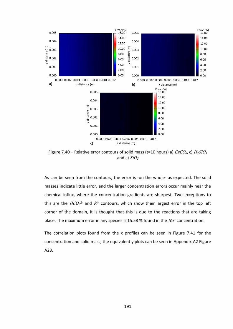
191
Figure 7.40 – Relative error contours of solid mass (t=10 hours) a) CaCO3, c) H4SiO4 and c) SiO2
As can be seen from the contours, the error is -on the whole- as expected. The solid
masses indicate little error, and the larger concentration errors occur mainly near the
chemical influx, where the concentration gradients are sharpest. Two exceptions to
this are the HCO32- and K+ contours, which show their largest error in the top left
corner of the domain, it is thought that this is due to the reactions that are taking
place. The maximum error in any species is 15.58 % found in the Na+ concentration.
The correlation plots found from the x profiles can be seen in Figure 7.41 for the
concentration and solid mass, the equivalent y plots can be seen in Appendix A2 Figure
A23.
a) b)
c)
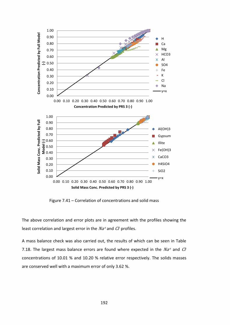
192
Figure 7.41 – Correlation of concentrations and solid mass
The above correlation and error plots are in agreement with the profiles showing the
least correlation and largest error in the Na+ and Cl- profiles.
A mass balance check was also carried out, the results of which can be seen in Table
7.18. The largest mass balance errors are found where expected in the Na+ and Cl-
concentrations of 10.01 % and 10.20 % relative error respectively. The solids masses
are conserved well with a maximum error of only 3.62 %.
0.00
0.10
0.20
0.30
0.40
0.50
0.60
0.70
0.80
0.90
1.00
0.00 0.10 0.20 0.30 0.40 0.50 0.60 0.70 0.80 0.90 1.00
Co
nce
ntr
atio
n P
red
icte
d b
y Fu
ll M
od
el
(-)
Concentration Predicted by PRS 3 (-)
H
Ca
Mg
HCO3
Al
SO4
Fe
K
Cl
Na
y=x
0.00
0.10
0.20
0.30
0.40
0.50
0.60
0.70
0.80
0.90
1.00
0.00 0.10 0.20 0.30 0.40 0.50 0.60 0.70 0.80 0.90 1.00
Solid
Mas
s C
on
c. P
red
icte
d b
y Fu
ll M
od
el (
-)
Solid Mass Conc. Predicted by PRS 3 (-)
Al(OH)3
Gypsum
Illite
Fe(OH)3
CaCO3
H4SiO4
SiO2
y=x
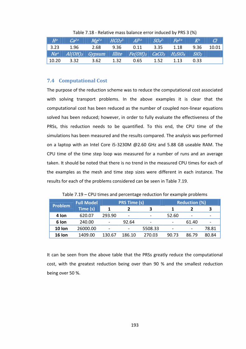
193
Table 7.18 - Relative mass balance error induced by PRS 3 (%)
H+ Ca2+ Mg2+ HCO32- Al3+ SO42- Fe3+ K+ Cl-
3.23 1.96 2.68 9.36 0.11 3.35 1.18 9.36 10.01
Na+ Al(OH)3 Gypsum Illite Fe(OH)3 CaCO3 H2SiO4 SiO2
10.20 3.32 3.62 1.32 0.65 1.52 1.13 0.33
7.4 Computational Cost
The purpose of the reduction scheme was to reduce the computational cost associated
with solving transport problems. In the above examples it is clear that the
computational cost has been reduced as the number of coupled non-linear equations
solved has been reduced; however, in order to fully evaluate the effectiveness of the
PRSs, this reduction needs to be quantified. To this end, the CPU time of the
simulations has been measured and the results compared. The analysis was performed
on a laptop with an Intel Core i5-3230M @2.60 GHz and 5.88 GB useable RAM. The
CPU time of the time step loop was measured for a number of runs and an average
taken. It should be noted that there is no trend in the measured CPU times for each of
the examples as the mesh and time step sizes were different in each instance. The
results for each of the problems considered can be seen in Table 7.19.
Table 7.19 – CPU times and percentage reduction for example problems
Problem Full Model
Time (s)
PRS Time (s) Reduction (%)
1 2 3 1 2 3
4 Ion 620.07 293.90 - - 52.60 - -
6 Ion 240.00 - 92.64 - - 61.40 -
10 Ion 26000.00 - - 5508.33 - - 78.81
16 Ion 1409.00 130.67 186.10 270.03 90.73 86.79 80.84
It can be seen from the above table that the PRSs greatly reduce the computational
cost, with the greatest reduction being over than 90 % and the smallest reduction
being over 50 %.
194
7.5 Investigation into the use of Analytical Relationships for the
Reduction Scheme
Before developing the numerically based PRSs, presented previously, an investigation
into the analytical relationship between the diffusion coefficient and the transport of a
species over a time step was made. The analytical solution considered can be found in
(Crank 1975), and is given for a semi-infinite medium as:
(
√ ) (7.11)
where x (>0) is the distance from the exposed face and erfc is the complimentary error
function. For this investigation, a problem concerning the 1D diffusion of ions into a
semi-infinite domain with a boundary concentration of 1 kg/kg was considered. The
analytical formula was used to calculate the transient diffusion of a number of species
with differing diffusion coefficients and the results used to analyse the relationship
between the transport over a time step and the diffusion coefficient relative to an
indicator species, such that the change in concentration ratio can be calculated as a
function of the diffusion coefficient ratio as follows:
(
) (7.12)
An investigation was also made into the dependence of this, if any, on the time t and
the distance from the boundary x. For the investigation, the indicator species had a
diffusion coefficient of 1x10⁻⁹ m2/s.
The first discovery was that if any species with a higher diffusion coefficient than the
indicator was included, the relationship of the concentration ratio to diffusion
coefficient tended to infinity, as can be seen in Figure 7.42. This makes sense at the
early stages of the problem since there would be some transport in the higher
diffusion coefficient species whilst the indicator species transport would be near to
zero.
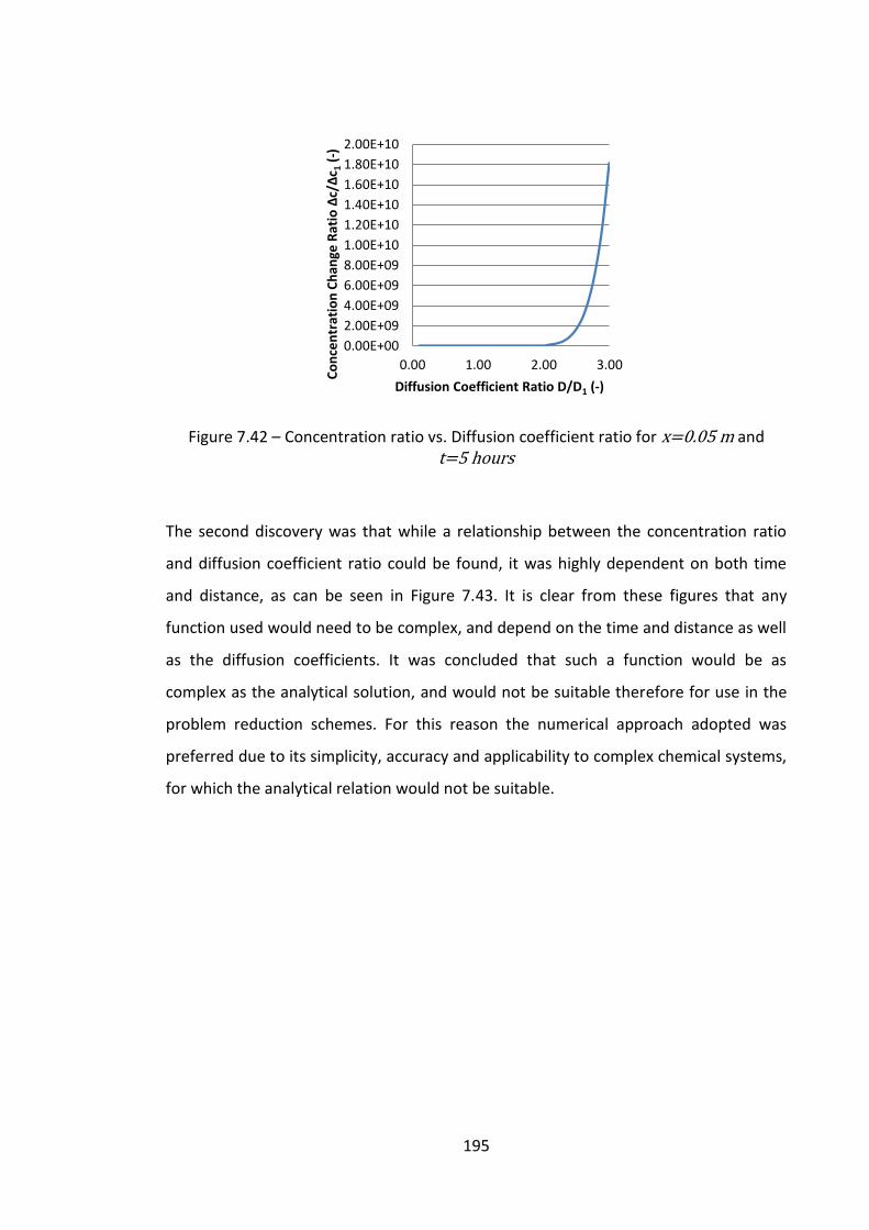
195
Figure 7.42 – Concentration ratio vs. Diffusion coefficient ratio for x=0.05 m and t=5 hours
The second discovery was that while a relationship between the concentration ratio
and diffusion coefficient ratio could be found, it was highly dependent on both time
and distance, as can be seen in Figure 7.43. It is clear from these figures that any
function used would need to be complex, and depend on the time and distance as well
as the diffusion coefficients. It was concluded that such a function would be as
complex as the analytical solution, and would not be suitable therefore for use in the
problem reduction schemes. For this reason the numerical approach adopted was
preferred due to its simplicity, accuracy and applicability to complex chemical systems,
for which the analytical relation would not be suitable.
0.00E+00
2.00E+09
4.00E+09
6.00E+09
8.00E+09
1.00E+10
1.20E+10
1.40E+10
1.60E+10
1.80E+10
2.00E+10
0.00 1.00 2.00 3.00
Co
nce
ntr
atio
n C
han
ge R
atio
Δc/Δ
c 1 (
-)
Diffusion Coefficient Ratio D/D1 (-)
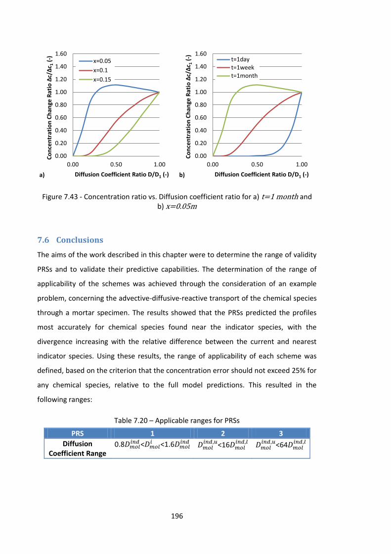
196
Figure 7.43 - Concentration ratio vs. Diffusion coefficient ratio for a) t=1 month and b) x=0.05m
7.6 Conclusions
The aims of the work described in this chapter were to determine the range of validity
PRSs and to validate their predictive capabilities. The determination of the range of
applicability of the schemes was achieved through the consideration of an example
problem, concerning the advective-diffusive-reactive transport of the chemical species
through a mortar specimen. The results showed that the PRSs predicted the profiles
most accurately for chemical species found near the indicator species, with the
divergence increasing with the relative difference between the current and nearest
indicator species. Using these results, the range of applicability of each scheme was
defined, based on the criterion that the concentration error should not exceed 25% for
any chemical species, relative to the full model predictions. This resulted in the
following ranges:
Table 7.20 – Applicable ranges for PRSs
PRS 1 2 3
Diffusion Coefficient Range
0.8 <
<1.6
, <16 ,
, <64 ,
0.00
0.20
0.40
0.60
0.80
1.00
1.20
1.40
1.60
0.00 0.50 1.00
Co
nce
ntr
atio
n C
han
ge R
atio
Δc/Δ
c 1 (
-)
Diffusion Coefficient Ratio D/D1 (-) a)
x=0.05
x=0.1
x=0.15
0.00
0.20
0.40
0.60
0.80
1.00
1.20
1.40
1.60
0.00 0.50 1.00
Co
nce
ntr
atio
n C
han
ge R
atio
Δc/Δ
c 1 (
-)
Diffusion Coefficient Ratio D/D1 (-) b)
t=1dayt=1weekt=1month
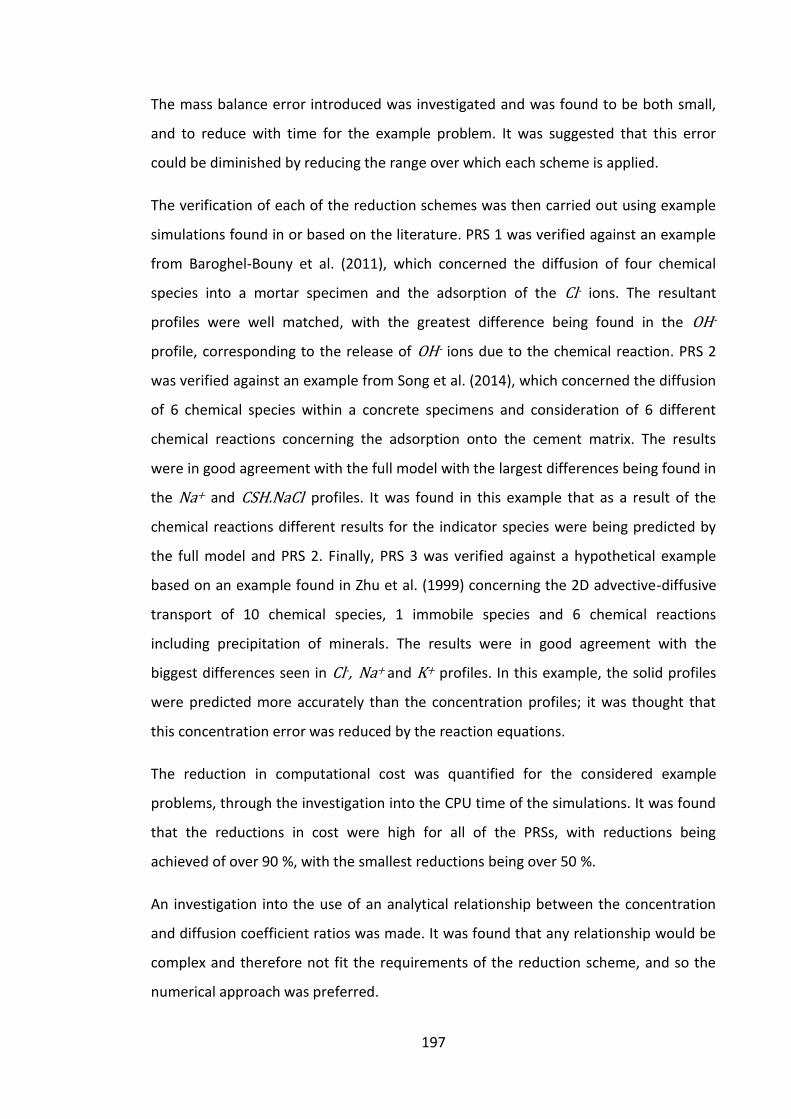
197
The mass balance error introduced was investigated and was found to be both small,
and to reduce with time for the example problem. It was suggested that this error
could be diminished by reducing the range over which each scheme is applied.
The verification of each of the reduction schemes was then carried out using example
simulations found in or based on the literature. PRS 1 was verified against an example
from Baroghel-Bouny et al. (2011), which concerned the diffusion of four chemical
species into a mortar specimen and the adsorption of the Cl- ions. The resultant
profiles were well matched, with the greatest difference being found in the OH-
profile, corresponding to the release of OH- ions due to the chemical reaction. PRS 2
was verified against an example from Song et al. (2014), which concerned the diffusion
of 6 chemical species within a concrete specimens and consideration of 6 different
chemical reactions concerning the adsorption onto the cement matrix. The results
were in good agreement with the full model with the largest differences being found in
the Na+ and CSH.NaCl profiles. It was found in this example that as a result of the
chemical reactions different results for the indicator species were being predicted by
the full model and PRS 2. Finally, PRS 3 was verified against a hypothetical example
based on an example found in Zhu et al. (1999) concerning the 2D advective-diffusive
transport of 10 chemical species, 1 immobile species and 6 chemical reactions
including precipitation of minerals. The results were in good agreement with the
biggest differences seen in Cl-, Na+ and K+ profiles. In this example, the solid profiles
were predicted more accurately than the concentration profiles; it was thought that
this concentration error was reduced by the reaction equations.
The reduction in computational cost was quantified for the considered example
problems, through the investigation into the CPU time of the simulations. It was found
that the reductions in cost were high for all of the PRSs, with reductions being
achieved of over 90 %, with the smallest reductions being over 50 %.
An investigation into the use of an analytical relationship between the concentration
and diffusion coefficient ratios was made. It was found that any relationship would be
complex and therefore not fit the requirements of the reduction scheme, and so the
numerical approach was preferred.

198
It is concluded from the work described in this chapter that each of the PRSs can
successfully be used to reduce the computational cost of a simulation whilst
maintaining a suitable accuracy of the results. The accuracy of the solutions can be
increased further by reducing the range of diffusion coefficients over which each
scheme is applied.
199
Chapter 8. Conclusions and Future Work
The work of this thesis had two main aims; firstly, to develop a numerical approach to
the problem size reduction that would reduce the computational demand associated
with the simulation of reactive transport problems; and secondly, to develop an
experimental test procedure for the investigation of transport behaviour in
cementitious materials, that allowed for different flow conditions and the
measurement of transient behaviour, without requiring the removal of the specimen
from the test setup. The development of a full coupled model, including the theory
upon which it is based and the numerical implementation, was presented in Chapters 3
and 4, with the problem reduction scheme being introduced in Chapter 4. The
development of the experimental procedure, including the test setup and concrete mix
design, was discussed in Chapter 5.
The conclusions of this thesis are directly linked to the objectives of the study, which
are recalled as:
1. Develop a coupled model based on a reliable mathematical framework for the
simulation of reactive transport problems in porous media.
2. Investigate the behaviour of the coupled model for different chemical systems,
including different boundary conditions, a range of transport behaviour and
various reactions to determine the validity of the model.
3. Propose a problem reduction scheme for use in complex multi-ionic systems in
order to reduce the computational cost of the simulations.
4. Investigate the problem reduction scheme through an example to determine
the range of applicability of each of the approaches, before investigating the
behaviour of the schemes for different chemical systems including different
boundary conditions, a range of transport behaviour and various reactions to
determine the validity of the approach.
5. Develop a simple alternative to column leaching tests for cementitious
materials using lab scale concrete beams and carry out tests in order to
determine different chemical parameters such as dispersion coefficients, as
well as providing data for the validation of the proposed model.
The summary of the work of this study is as follows:
200
The mathematical framework upon which the model is based allows for its
application to different porous media and a range of chemical systems,
including different reaction chemistry and multi-ionic transport. In terms of
moisture transport, the model was found to perform well in the prediction of
the moisture loss of drying experiments, and predicted accurate transient
profiles of the moisture at near to the exposed face. The profile at the interior
of the specimens however was under predicted following the initial drying
period.
In a numerically based drying example good agreement was obtained between
the prediction of the moisture profiles of the current model and the results
from Koniorczyk and Gawin (2012). Greater discrepancies in the prediction of
the moisture profiles were found between the model and the results of
Koniorczyk (2010). The general trend was in agreement, however the shape of
the profiles was not. It was not clear in these examples however which values
of the parameters of the moisture flow were used.
The reactive chemical transport was validated against the experimental results,
as well as verified against a number of examples from Baroghel-Bouny et al.
(2011) and Song et al. (2014). It was found that the model accurately predicted
both the concentration and solid mass profiles and their transient behaviour.
The largest differences occurred either when the values of the reaction
parameters were unclear, or the chemical in question was found in small
concentrations and therefore was perhaps more sensitive to error.
Three different problem reduction schemes were proposed, each of differing
complexity, and each using a different number of indicator species. An
investigation was made into the range of validity of each of the reduction
schemes through an example problem concerning the advective diffusive
reactive transport of 16 chemical species into a mortar specimen. It was found
that the schemes had an increasing range of applicability and that PRS 3
covered the whole range of diffusion coefficients considered, which was higher
than would normally be found in a real chemical system.

201
Each of the reduction schemes were then verified using a single example
problem. It was found that the reduction schemes accurately captured the
chemical behaviour whilst reducing the number of coupled equations to be
solved. The computational cost was investigated in terms of CPU time, which
was found to be up to over 90 %.
The mass balance error introduced through the use of the reduction schemes
was investigated, with the maximum for the 16 ion example being around 10 %
and showing a decrease with time.
A simple approach to ion transport experiments was developed through the
use of Perspex tanks that allow different heads of water, connected by a sealed
concrete beam. The measurements of concentration were taken through the
extraction of a pore water sample using a syringe and the tests were
accelerated through the design of a porous concrete mix. It was found that the
experiments were successful in providing results for the concentration profiles
of a salt. A number of problems were encountered throughout the
development, the main one being the leaking of the tanks through the seal of
the concrete beams to the specimen.
The conclusions of this study are as follows:
1. The full model is able to accurately reproduce the results of experiments and
alternative numerical models considering the reactive transport behaviour.
2. The problem reduction schemes were able to accurately capture the transport
behaviour as predicted by the full model, whilst achieving reductions in cost of
up to 90 % CPU time.
3. The ion transport experiments were successful in providing a simple solution to
the problems associated with current approaches. The results obtained,
however, were limited.
The suggestions for future research from this study are as follows:
1. Further investigation needs to be made into the performance of the PRSs
including both:
202
a. The validity of the ranges of applicability for different chemical and flow
conditions as these may have an effect on the range of diffusion
coefficients over which the schemes give accurate results.
b. The mass balance error introduced by the PRSs for different chemical
and flow conditions, with particular attention directed to its changes
over time.
2. Concerning the ion transport experiments, further investigation is needed into
different ways of sealing the beam in place to reduce the occurrence of leaks. It
is thought that the use of a rubber gasket may provide an easier and more
consistent way of sealing the beams into place.
The suggestions for future research based on the scope and limitations of this study
are as follows:
1. The reactions considered were all kinetic and therefore an investigation is
needed into the behaviour of the PRSs under chemical equilibrium conditions.
Equilibrium reactions are found in a number of chemical systems in both
cementitious materials and soils. The inclusion of equilibrium reactions would
greatly widen the range of problems and applications for which the PRSs could
be used (particularly for geochemical problems where equilibrium reactions are
commonly used).
2. The example problems considered did not include temperature changes and
neglected the enthalpy change of reactions; further investigation is therefore
needed into this area. There is also coupling between the temperature and the
chemistry (for example the rate of reactions which depend on temperature,
enthalpy change of reactions, and effect of precipitated materials on specific
heat of the medium). It is therefore important to investigate the sensitivity of
the temperature to the problem chemistry to determine the effect of using the
PRSs on the accuracy of the temperature profiles.
3. The effect of the dependence of the diffusion coefficients on both the degree
of saturation and the chemical concentration should be investigated. As well as
the effect of the chemical activity of the pore water on the transport

203
mechanisms should be investigated. This is important to determine the
performance of the PRSs with an increased degree of coupling between the
moisture and chemical phases.

204
205
References
Ahmad, S. and Azad, a 2013. An exploratory study on correlating the permeability of concrete with its porosity and tortuosity. Advances in Cement Research 25(5), pp. 288–294.
Al-amoudi, O.S.B., Al-kutti, W.A., Ahmad, S. and Maslehuddin, M. 2009. Correlation between compressive strength and certain durability indices of plain and blended cement concretes. Cement and Concrete Composites 31(9), pp. 672–676. Available at: http://dx.doi.org/10.1016/j.cemconcomp.2009.05.005.
Aliko-Benítez, A., Doblaré, M. and Sanz-Herrera, J.A. 2015. Chemical-diffusive modelling of the self-healing behavior in concrete. International Journal of Solids and Structures 70, pp. 392–402. Available at: http://www.sciencedirect.com/science/article/pii/S0020768315002218.
Allison, J.D., Brown, D.S. and Novo-Gradac, K.J. 1991. Minteqa2/Prodefa2, a Geochemical Assessment Model for Environmental Systems: Version 3.0 User’S Manual. U. S. Environmental Protection Agency EPA/600/3-91/021 (March), p. 115.
Ashby, S.F. and Falgout, R.D. 1996. A parallel multigrid preconditioned conjugate gradient algorithm for groundwater flow simulations. Nuclear Science and Engineering 124, pp. 145–159. Available at: http://cat.inist.fr/?aModele=afficheN&cpsidt=3247969.
Baroghel-Bouny, V., Belin, P., Maultzsch, M. and Henry, D. 2007a. AgNO 3 spray tests : advantages , weaknesses , and various applications to quantify chloride ingress into concrete . Part 1 : AgNO 3 spray tests : advantages , weaknesses , and various applications. Materials and structures (2007), pp. 759–781.
Baroghel-Bouny, V., Belin, P., Maultzsch, M. and Henry, D. 2007b. AgNO 3 spray tests : advantages , weaknesses , and various applications to quantify chloride ingress into concrete . Part 2 : Non-steady-state migration tests and chloride diffusion coefficients. Materials and structures (2007), pp. 759–781.
Baroghel-Bouny, V., Kinomura, K., Thiery, M. and Moscardelli, S. 2011. Easy assessment of durability indicators for service life prediction or quality control of concretes with high volumes of supplementary cementitious materials. Cement and Concrete Composites 33(8), pp. 832–847. Available at: http://dx.doi.org/10.1016/j.cemconcomp.2011.04.007.
Baroghel-Bouny, V., Nguyen, T.Q. and Dangla, P. 2009. Assessment and prediction of RC structure service life by means of durability indicators and physical/chemical models. Cement and Concrete Composites 31(8), pp. 522–534. Available at: http://dx.doi.org/10.1016/j.cemconcomp.2009.01.009.
Baroghel-Bouny, V., Thiéry, M. and Wang, X. 2011. Modelling of isothermal coupled moisture-ion transport in cementitious materials. Cement and Concrete Research 41(8), pp. 828–841. Available at: http://dx.doi.org/10.1016/j.cemconres.2011.04.001.
Baroghel-Bouny, V., Wang, X., Thiery, M., Saillio, M. and Barberon, F. 2012. Prediction of chloride binding isotherms of cementitious materials by ‘analytical’ model or
206
‘numerical’ inverse analysis. Cement and Concrete Research 42(9), pp. 1207–1224. Available at: http://dx.doi.org/10.1016/j.cemconres.2012.05.008.
Bary, B., Ranc, G., Durand, S. and Carpentier, O. 2008. A coupled thermo-hydro-mechanical-damage model for concrete subjected to moderate temperatures. International Journal of Heat and Mass Transfer 51(11–12), pp. 2847–2862.
Bear, J. and Bachmat, Y. 1990. Introduction to modelling of transport phenomena in porous media. The Netherlands: Kluwer Academic Publishers.
Bear, J. and Verruijt, A. 1987. Modelling Groundwater Flow and Pollution. The Netherlands: D. Reidel Publishing Company.
Beisman, J.J., Maxwell, R.M., Navarre-Sitchler, A.K., Steefel, C.I. and Molins, S. 2015. ParCrunchFlow: an efficient, parallel reactive transport simulation tool for physically and chemically heterogeneous saturated subsurface environments. Computational Geosciences 19(2), pp. 403–422.
Bertocchi, A.F., Ghiani, M., Peretti, R. and Zucca, A. 2006. Red mud and fly ash for remediation of mine sites contaminated with As, Cd, Cu, Pb and Zn. Journal of Hazardous Materials 134(1–3), pp. 112–119.
Boggs, J.M. and Adams, E.E. 1992. Field study of dispersion in a heterogeneous aquifer 4. Investigation of adsorption and sampling bias. Water Resources Research 28(12), pp. 3325–3336.
British Standards Institution. 2013. BS EN 12620:2013. Aggregates for concrete. London: BSI.
Brooks, R.H. and Corey, a T. 1964. Hydraulic properties of porous media. Hydrology Papers, Colorado State University. Fort Collins CO 3(3), p. 27 pgs.
Buckingham, E. 1907. Studies on the movement of soil moisture. Bull. 38. Washington D.C.: USDA, Bureau of Soils.
Carrayrou, J., Kern, M. and Knabner, P. 2010. Reactive transport benchmark of MoMaS. Computational Geosciences 14(3), pp. 385–392. Available at: http://dx.doi.org/10.1007/s10596-009-9157-7.
Chitez, A.S. and Jefferson, A.D. 2015. Porosity development in a thermo-hygral finite element model for cementitious materials. Cement and Concrete Research 78, pp. 216–233. Available at: http://dx.doi.org/10.1016/j.cemconres.2015.07.010.
Chitez, A.S. and Jefferson, A.D. 2016. A coupled thermo-hygro-chemical model for characterising autogenous healing in ordinary cementitious materials. Cement and Concrete Research 88, pp. 184–197. Available at: http://dx.doi.org/10.1016/j.cemconres.2016.07.002.
Cleall, P.J. 1998. An investigation into the thermo/hydraulic/mechanical behaviour of unsaturated soils, including expansive clays. Cardiff University.
Cleall, P.J., Seetharam, S.C. and Thomas, H.R. 2007. Inclusion of Some Aspects of
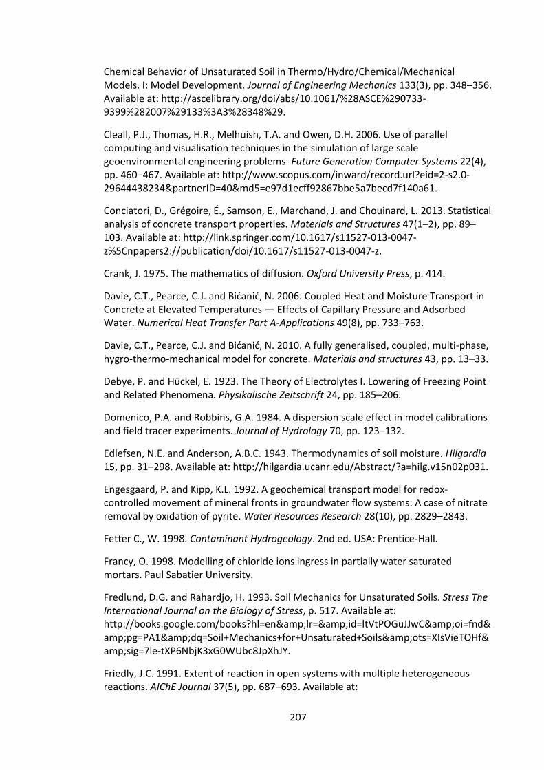
207
Chemical Behavior of Unsaturated Soil in Thermo/Hydro/Chemical/Mechanical Models. I: Model Development. Journal of Engineering Mechanics 133(3), pp. 348–356. Available at: http://ascelibrary.org/doi/abs/10.1061/%28ASCE%290733-9399%282007%29133%3A3%28348%29.
Cleall, P.J., Thomas, H.R., Melhuish, T.A. and Owen, D.H. 2006. Use of parallel computing and visualisation techniques in the simulation of large scale geoenvironmental engineering problems. Future Generation Computer Systems 22(4), pp. 460–467. Available at: http://www.scopus.com/inward/record.url?eid=2-s2.0-29644438234&partnerID=40&md5=e97d1ecff92867bbe5a7becd7f140a61.
Conciatori, D., Grégoire, É., Samson, E., Marchand, J. and Chouinard, L. 2013. Statistical analysis of concrete transport properties. Materials and Structures 47(1–2), pp. 89–103. Available at: http://link.springer.com/10.1617/s11527-013-0047-z%5Cnpapers2://publication/doi/10.1617/s11527-013-0047-z.
Crank, J. 1975. The mathematics of diffusion. Oxford University Press, p. 414.
Davie, C.T., Pearce, C.J. and Bićanić, N. 2006. Coupled Heat and Moisture Transport in Concrete at Elevated Temperatures — Effects of Capillary Pressure and Adsorbed Water. Numerical Heat Transfer Part A-Applications 49(8), pp. 733–763.
Davie, C.T., Pearce, C.J. and Bićanić, N. 2010. A fully generalised, coupled, multi-phase, hygro-thermo-mechanical model for concrete. Materials and structures 43, pp. 13–33.
Debye, P. and Hückel, E. 1923. The Theory of Electrolytes I. Lowering of Freezing Point and Related Phenomena. Physikalische Zeitschrift 24, pp. 185–206.
Domenico, P.A. and Robbins, G.A. 1984. A dispersion scale effect in model calibrations and field tracer experiments. Journal of Hydrology 70, pp. 123–132.
Edlefsen, N.E. and Anderson, A.B.C. 1943. Thermodynamics of soil moisture. Hilgardia 15, pp. 31–298. Available at: http://hilgardia.ucanr.edu/Abstract/?a=hilg.v15n02p031.
Engesgaard, P. and Kipp, K.L. 1992. A geochemical transport model for redox‐controlled movement of mineral fronts in groundwater flow systems: A case of nitrate removal by oxidation of pyrite. Water Resources Research 28(10), pp. 2829–2843.
Fetter C., W. 1998. Contaminant Hydrogeology. 2nd ed. USA: Prentice-Hall.
Francy, O. 1998. Modelling of chloride ions ingress in partially water saturated mortars. Paul Sabatier University.
Fredlund, D.G. and Rahardjo, H. 1993. Soil Mechanics for Unsaturated Soils. Stress The International Journal on the Biology of Stress, p. 517. Available at: http://books.google.com/books?hl=en&lr=&id=ltVtPOGuJJwC&oi=fnd&pg=PA1&dq=Soil+Mechanics+for+Unsaturated+Soils&ots=XIsVieTOHf&sig=7le-tXP6NbjK3xG0WUbc8JpXhJY.
Friedly, J.C. 1991. Extent of reaction in open systems with multiple heterogeneous reactions. AIChE Journal 37(5), pp. 687–693. Available at:
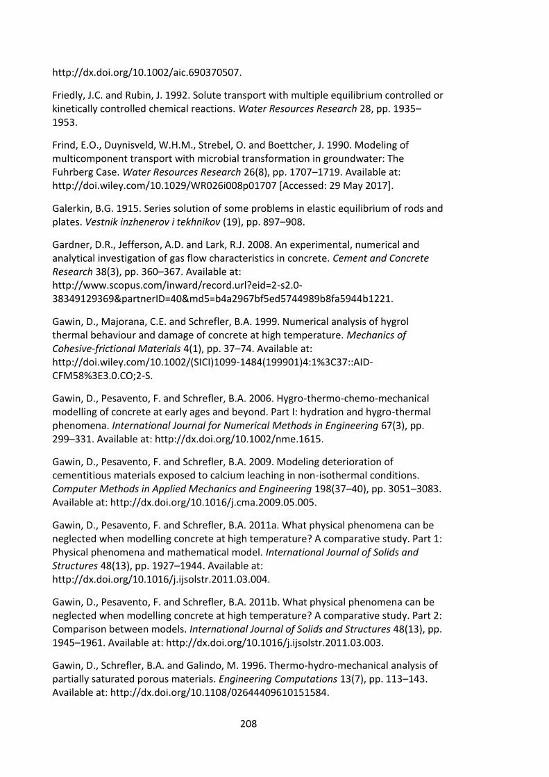
208
http://dx.doi.org/10.1002/aic.690370507.
Friedly, J.C. and Rubin, J. 1992. Solute transport with multiple equilibrium controlled or kinetically controlled chemical reactions. Water Resources Research 28, pp. 1935–1953.
Frind, E.O., Duynisveld, W.H.M., Strebel, O. and Boettcher, J. 1990. Modeling of multicomponent transport with microbial transformation in groundwater: The Fuhrberg Case. Water Resources Research 26(8), pp. 1707–1719. Available at: http://doi.wiley.com/10.1029/WR026i008p01707 [Accessed: 29 May 2017].
Galerkin, B.G. 1915. Series solution of some problems in elastic equilibrium of rods and plates. Vestnik inzhenerov i tekhnikov (19), pp. 897–908.
Gardner, D.R., Jefferson, A.D. and Lark, R.J. 2008. An experimental, numerical and analytical investigation of gas flow characteristics in concrete. Cement and Concrete Research 38(3), pp. 360–367. Available at: http://www.scopus.com/inward/record.url?eid=2-s2.0-38349129369&partnerID=40&md5=b4a2967bf5ed5744989b8fa5944b1221.
Gawin, D., Majorana, C.E. and Schrefler, B.A. 1999. Numerical analysis of hygrol thermal behaviour and damage of concrete at high temperature. Mechanics of Cohesive‐frictional Materials 4(1), pp. 37–74. Available at: http://doi.wiley.com/10.1002/(SICI)1099-1484(199901)4:1%3C37::AID-CFM58%3E3.0.CO;2-S.
Gawin, D., Pesavento, F. and Schrefler, B.A. 2006. Hygro-thermo-chemo-mechanical modelling of concrete at early ages and beyond. Part I: hydration and hygro-thermal phenomena. International Journal for Numerical Methods in Engineering 67(3), pp. 299–331. Available at: http://dx.doi.org/10.1002/nme.1615.
Gawin, D., Pesavento, F. and Schrefler, B.A. 2009. Modeling deterioration of cementitious materials exposed to calcium leaching in non-isothermal conditions. Computer Methods in Applied Mechanics and Engineering 198(37–40), pp. 3051–3083. Available at: http://dx.doi.org/10.1016/j.cma.2009.05.005.
Gawin, D., Pesavento, F. and Schrefler, B.A. 2011a. What physical phenomena can be neglected when modelling concrete at high temperature? A comparative study. Part 1: Physical phenomena and mathematical model. International Journal of Solids and Structures 48(13), pp. 1927–1944. Available at: http://dx.doi.org/10.1016/j.ijsolstr.2011.03.004.
Gawin, D., Pesavento, F. and Schrefler, B.A. 2011b. What physical phenomena can be neglected when modelling concrete at high temperature? A comparative study. Part 2: Comparison between models. International Journal of Solids and Structures 48(13), pp. 1945–1961. Available at: http://dx.doi.org/10.1016/j.ijsolstr.2011.03.003.
Gawin, D., Schrefler, B.A. and Galindo, M. 1996. Thermo‐hydro‐mechanical analysis of partially saturated porous materials. Engineering Computations 13(7), pp. 113–143. Available at: http://dx.doi.org/10.1108/02644409610151584.
209
Gens, A., do N. Guimarães, L., Olivella, S. and Sánchez, M. 2004. Analysis of the Thmc Behaviour of Compacted Swelling Clay for Radioactive Waste Isolation. In: Stephanson, O. ed. Coupled Thermo-Hydro-Mechanical-Chemical Processes in Geo-SystemsFundamentals, Modelling, Experiments and Applications. Elsevier Geo-Engineering Book Series. Elsevier, pp. 317–322.
van Genuchten, M.T. 1980. A Closed-form Equation for Predicting the Hydraulic Conductivity of Unsaturated Soils. Soil Science Society of America Journal 44(5), p. 892.
Hartley, W., Edwards, R. and Lepp, N.W. 2004. Arsenic and heavy metal mobility in iron oxide-amended contaminated soils as evaluated by short- and long-term leaching tests. Environmental Pollution 131(3), pp. 495–504.
Hassanizadeh, M. and Gray, W.G. 1979. General conservation equations for multi-phase systems: 1. Averaging procedure. Advances in Water Resources 2(C), pp. 131–144.
Hillel, D. 1980. Fundamentals of soil physics. San Diego, Calif.: Academic.
Hoffmann, J., Kräutle, S. and Knabner, P. 2012. A general reduction scheme for reactive transport in porous media. Computational Geosciences 16(4), pp. 1081–1099.
Huo, J.X., Song, H.Z. and Wu, Z.W. 2014. Multi-component reactive transport in heterogeneous media and its decoupling solution. Journal of Contaminant Hydrology 166, pp. 11–22. Available at: http://dx.doi.org/10.1016/j.jconhyd.2014.07.009.
Irmay, S. 1954. On the hydraulic conductivity of unsaturated soils. Eos, Transactions American Geophysical Union 35(3), pp. 1–5.
Khan, A.U.H. and Jury, W.A. 1990. A laboratory study of the dispersion scale effect in column outflow experiments. Journal of Contaminant Hydrology 5(2), pp. 119–131.
Kim, J.K. and Lee, C.S. 1999. Moisture diffusion of concrete considering self-desiccation at early ages. Cement and Concrete Research 29(12), pp. 1921–1927.
Kim, Y.Y., Lee, K.M., Bang, J.W. and Kwon, S.J. 2014. Effect of W/C ratio on durability and porosity in cement mortar with constant cement amount. Advances in Materials Science and Engineering 2014.
Koniorczyk, M. 2010. Modelling the phase change of salt dissolved in pore water - Equilibrium and non-equilibrium approach. Construction and Building Materials 24(7), pp. 1119–1128. Available at: http://dx.doi.org/10.1016/j.conbuildmat.2009.12.031.
Koniorczyk, M. 2012. Salt transport and crystallization in non-isothermal, partially saturated porous materials considering ions interaction model. International Journal of Heat and Mass Transfer 55(4), pp. 665–679. Available at: http://dx.doi.org/10.1016/j.ijheatmasstransfer.2011.10.043.
Koniorczyk, M. and Gawin, D. 2008. Heat and Moisture Transport in Porous Building Materials Containing Salt. Journal of Building Physics 31(4), pp. 279–300.
Koniorczyk, M. and Gawin, D. 2011. Numerical Modeling of Salt Transport and
210
Precipitation in Non-Isothermal Partially Saturated Porous Media Considering Kinetics of Salt Phase Changes. Transport in Porous Media 87(1), pp. 57–76.
Koniorczyk, M. and Gawin, D. 2012. Modelling of salt crystallization in building materials with microstructure - Poromechanical approach. Construction and Building Materials 36, pp. 860–873. Available at: http://dx.doi.org/10.1016/j.conbuildmat.2012.06.035.
Koniorczyk, M., Gawin, D. and Schrefler, B.A. 2015. Modeling evolution of frost damage in fully saturated porous materials exposed to variable hygro-thermal conditions. Computer Methods in Applied Mechanics and Engineering 297, pp. 38–61. Available at: http://dx.doi.org/10.1016/j.cma.2015.08.015.
Koniorczyk, M. and Wojciechowski, M. 2009. Influence of salt on desorption isotherm and hygral state of cement mortar - Modelling using neural networks. Construction and Building Materials 23(9), pp. 2988–2996. Available at: http://dx.doi.org/10.1016/j.conbuildmat.2009.05.001.
Kräutle, S. 2008. General Multi-Species Reactive Transport Problems in Porous Media : Efficient Numerical Approaches and Existence of Global Solutions.
Kräutle, S. and Knabner, P. 2005. A new numerical reduction scheme for fully coupled multicomponent transport-reaction problems in porous media. Water Resources Research 41(9), pp. 1–17.
Kräutle, S. and Knabner, P. 2007. A reduction scheme for coupled multicomponent transport-reaction problems in porous media: Generalization to problems with heterogeneous equilibrium reactions. Water Resources Research 43(3).
Krueger, C.J., Radakovich, K.M., Sawyer, T.E., Barber, L.B., Smith, R.L. and Field, J.A. 1998. Biodegradation of the surfactant linear alkylbenzenesulfonate in sewage- contaminated groundwater: A comparison of column experiments and field tracer tests. Environmental Science and Technology 32(24), pp. 3954–3961.
Kuhl, D., Bangert, F. and Meschke, G. 2004. Coupled chemo-mechanical deterioration of cementitious materials. Part I: Modeling. International Journal of Solids and Structures 41(1), pp. 15–40.
Kulik, D.A., Wagner, T., Dmytrieva, S. V, Kosakowski, G., Hingerl, F.F., Chudnenko, K. V and Berner, U. 2012. GEM-Selektor geochemical modeling package: Numerical kernel GEMS3K for coupled simulation codes. Computational Geosciences 17(1), pp. 1–24.
Lagneau, V. and van der Lee, J. 2010. HYTEC results of the MoMaS reactive transport benchmark. Computational Geosciences 14(3), pp. 435–449.
Lasaga, A.C. 1981. The treatment of multicomponent diffusion and ion pairs in diagenetic fluxes: further comments and clarification. American Journal of Science 281(7), pp. 981–988.
Lewis, G.N., Randall, M., Pitzer, K.S. and Brewer, L. 1961. Thermodynamics. 2nd edition. New York, N.Y.: McGraw Hill.
211
Lewis R., W. and Schrefler B., A. 1998. The finite element method in the static and dynamic deformation and consolidation of porous media. 2nd ed. Great Britian: John Wiley and Sons Inc.
Lichtner, P.C. 1985. Continuum model for simultaneous chemical reactions and mass transport in hydrothermal systems. Geochimica et Cosmochimica Acta 49(3), pp. 779–800.
Liu, D., Jivkov, A.P., Wang, L., Si, G. and Yu, J. 2017. Non-Fickian dispersive transport of strontium in laboratory-scale columns: Modelling and evaluation. Journal of Hydrology 549, pp. 1–11. Available at: http://linkinghub.elsevier.com/retrieve/pii/S0022169417302032.
Matthäi, S.K., Geiger, S. and Roberts, S.G. 2001. Complex Systems Platform CSP3D3.0. (c).
Mayer, K.U. and MacQuarrie, K.T.B. 2010. Solution of the MoMaS reactive transport benchmark with MIN3P---model formulation and simulation results. Computational Geosciences 14(3), pp. 405–419. Available at: http://dx.doi.org/10.1007/s10596-009-9158-6.
McCutcheon, S.C., Martin, J.L. and Barnwell, T.O.J. 1993. Water Quality. In: Maidment, D. R. ed. Handbook of Hydrology. McGraw-Hill, pp. 346–414.
Mitchell, J.K. 1993. Fundamentals of Soil Behavior. Wiley.
Molins, S., Carrera, J., Ayora, C. and Saaltink, M.W. 2004. A formulation for decoupling components in reactive transport problems. Water Resources Research 40(10), pp. 1–13.
de Morais, M.V.G., Bary, B., Ranc, G., Pont, S.D. and Durand, S. 2009. Comparative Analysis of Coupled Thermo-Hydro-Mechanical Models for Concrete Exposed to Moderate Temperatures. Numerical Heat Transfer Part A-Applications 55(7), pp. 654–682. Available at: http://www.informaworld.com/smpp/content~db=all?content=10.1080/10407780902821516%5Cnpapers2://publication/doi/10.1080/10407780902821516.
Mualem, Y. 1976. A new model for predicting the hydraulic conductivity of unsaturated porous media. Water Resources Research 12(3), pp. 564–566.
Neithalath, N., Weiss, J. and Olek, J. 2006. Characterizing Enhanced Porosity Concrete using electrical impedance to predict acoustic and hydraulic performance. Cement and Concrete Research 36(11), pp. 2074–2085.
Netherlands Standardisation Institute. 1995. NEN 7473. Leaching Characteristics of Solid Earthy and Stony Building and Waste Materials. Leaching Tests. Determination of the Leaching of Inorganic Components from Granular Materials with the Column Test. Delft: NEN.
Nitao, J.J. and Bear, J. 1996. Potentials and their role in transport in porous media. Water Resources Research 32(2), pp. 225–250. Available at:
212
http://www.scopus.com/inward/record.url?eid=2-s2.0-0029744202&partnerID=40&md5=70ddc224a11eeeb3f42606fad3f3f752.
Nordtest. 1999. NT Build 492. Concrete, mortar and cement-based repair materials: Chloride migration coefficient from non-steady-state migration experiments. Espoo: Nordtest.
Parkhurst, D. l., Kipp, K. l. and Charlton, S. r. 2010. PHAST Version 2 - A program for simulating groundwater flow, solute transport, and multicomponent geochemical reactions. Modeling Techniques, Book 6, pp. 1–181. Available at: http://pubs.usgs.gov/tm/06A35/.
Parkhurst, D.L. and Wissmeier, L. 2015. PhreeqcRM: A reaction module for transport simulators based on the geochemical model PHREEQC. Advances in Water Resources 83, pp. 176–189. Available at: http://www.sciencedirect.com/science/article/pii/S0309170815001268.
Philip, J.R. and De Vries, D.A. 1957. Moisture movement in porous materials under temperature gradients. Eos, Transactions American Geophysical Union 38(2), pp. 222–232.
Pitzer, K.S. 1973. Thermodynamics of Electrolytes. I. Theoretical Basis and General Equations. The Journal of Physical Chemistry 77(2), pp. 268–277. Available at: http://pubs.acs.org/doi/abs/10.1021/j100621a026.
Pitzer, K.S. and Mayorga, G. 1973. Thermodynamics of electrolytes II. Activity and osmotic coefficients for strong electrolytes with one or both ions univalent. Journal of Chemical Information and Modeling 77(19), pp. 2300–2308.
Rees, S.W., Adjali, M.H., Zhou, Z., Davies, M. and Thomas, H.R. 2000. Ground heat transfer effects on the thermal performance of earth-contact structures. Renewable & sustainable energy reviews 4(3), pp. 213–265.
Richards, L.A. 1931. Capillary conduction of liquids through porous mediums. Journal of Applied Physics 1(5), pp. 318–333.
Robbins, G.A. 1989. Methods for determining transverse dispersion coefficients of porous media in laboratory column experiments. Water Resources Research 25(6), pp. 1249–1258.
Rubin, J. 1983. Transport of reacting solutes in porous media: Relation between mathematical nature of problem formulation and chemical nature of reactions. Water Resources Research 19(5), pp. 1231–1252.
Rubin, J. and James, R. V 1973. Dispersion-affected transport of reactive solutes in saturated porous media: Galerkin method applied to equilibrium-controlled exchange in unidirectional steady state water flow. Water Resour. Res. 9(5), pp. 1332–1356.
Saaltink, M.W., Carrera, J. and Ayora, C. 2001. On the behavior of approaches to simulate reactive transport. Journal of Contaminant Hydrology 48(3–4), pp. 213–235.
213
Samson, E. and Marchand, J. 2007a. Modeling the effect of temperature on ionic transport in cementitious materials. Cement and Concrete Research 37(3), pp. 455–468.
Samson, E. and Marchand, J. 2007b. Modeling the transport of ions in unsaturated cement-based materials. Computers and Structures 85(23–24), pp. 1740–1756.
De Schutter, G. and Taerwe, L. 1995. General hydration model for portland cement and blast furnace slag cement. Cement and Concrete Research 25(3), pp. 593–604.
Song, H.W., Lee, C.H. and Ann, K.Y. 2008. Factors influencing chloride transport in concrete structures exposed to marine environments. Cement and Concrete Composites 30(2), pp. 113–121.
Song, Z., Jiang, L., Chu, H., Xiong, C., Liu, R. and You, L. 2014. Modeling of chloride diffusion in concrete immersed in CaCl2 and NaCl solutions with account of multi-phase reactions and ionic interactions. Construction and Building Materials 66, pp. 1–9. Available at: http://dx.doi.org/10.1016/j.conbuildmat.2014.05.026.
Steefel, C.I., Appelo, C.A.J., Arora, B., Jacques, D., Kalbacher, T., Kolditz, O., Lagneau, V., Lichtner, P.C., et al. 2015. Reactive transport codes for subsurface environmental simulation.
Steiger, M., Kiekbusch, J. and Nicolai, A. 2008. An improved model incorporating Pitzer’s equations for calculation of thermodynamic properties of pore solutions implemented into an efficient program code. Construction and Building Materials 22(8), pp. 1841–1850.
Sun, G., Zhang, Y., Sun, W., Liu, Z. and Wang, C. 2011. Multi-scale prediction of the effective chloride diffusion coefficient of concrete. Construction and Building Materials 25(10), pp. 3820–3831. Available at: http://dx.doi.org/10.1016/j.conbuildmat.2011.03.041.
Thomas, H.R., Cleall, P.J., Li, Y., Harris, C. and Kern-Luetschg, M. 2009. Modelling of cryogenic processes in permafrost and seasonally frozen soils. Geotechnique (3), pp. 173–184. Available at: http://orca.cf.ac.uk/8408/.
Thomas, H.R. and He, Y. 1995. Analysis of coupled heat, moisture and air transfer in a deformable unsaturated soil. Géotechnique 45(4), pp. 677–689. Available at: http://dx.doi.org/10.1680/geot.1995.45.4.677.
Thomas, H.R. and He, Y. 1997. A coupled heat–moisture transfer theory for deformable unsaturated soil and its algorithmic implementation. International Journal for Numerical Methods in Engineering 40(18), pp. 3421–3441. Available at: http://dx.doi.org/10.1002/(SICI)1097-0207(19970930)40:18%3C3421::AID-NME220%3E3.0.CO;2-C%5Cnhttp://onlinelibrary.wiley.com/store/10.1002/(SICI)1097-0207(19970930)40:18%3C3421::AID-NME220%3E3.0.CO;2-C/asset/220_ftp.pdf?v=1&t=hd68fgbc&s=eda2fdc2a06a854b1c67.
Thomas, H.R., Sedighi, M. and Vardon, P.J. 2012. Diffusive Reactive Transport of Multicomponent Chemicals Under Coupled Thermal, Hydraulic, Chemical and
214
Mechanical Conditions. Geotechnical and Geological Engineering 30(4), pp. 841–857.
Thompson, J.B. 1982a. Composition space; an algebraic and geometric approach. Reviews in Mineralogy and Geochemistry 10(1), pp. 1–31. Available at: http://rimg.geoscienceworld.org/content/10/1/1.
Thompson, J.B. 1982b. Reaction space; an algebraic and geometric approach. Reviews in Mineralogy and Geochemistry 10(1), pp. 33–52. Available at: http://rimg.geoscienceworld.org/content/10/1/33.
Tie-hang, W. and Li-jun, S. 2009. Equation for Calculating Change in Moisture Content Caused by Water Vapor Transfer in Unsaturated Soil. Journal of Hydrologic Engineering 14(11), pp. 1235–1239.
Truc, O., Ollivier, J.P. and Carcassès, M. 2000. New way for determining the chloride diffusion coefficient in concrete from steady state migration test. Cement and Concrete Research 30(2), pp. 217–226.
Valocchi, A.J. and Malmstead, M. 1992. Accuracy of operator splitting for Advection-Dispersion-Reaction Problems. Water Resources Research 28(5), pp. 1471–1476.
Valocchi, A.J., Street, R.L. and Roberts, P. V 1981. Transport of ion-exchanging solutes in groundwater: Chromatogrphoc theory and field simulation. Water Resources Research 17(5), pp. 1517–1527.
Walter, A.L., Frind, E.O., Blowes, D.W., Ptacek, C.J. and Molson, J.W. 1994. Modeling of multicomponent reactive transport in groundwater. 1.Model development and evaluation. Water Resources Research 30(1), pp. 3137–3148.
Wierenga, P.J. and Van Genuchten, M.T. 1989. Solute transport through small and large unsaturated soil columns. Ground Water 27(1), pp. 35–42.
Xu, T., Spycher, N. and Sonnenthal, E. 2012. TOUGHREACT User’s Guide: A Simulation Program for Non-isothermal Multiphase Reactive Transport in Variably Saturated Geologic Media, version 2.0. Lawrence Berkeley … (October), pp. 1–5. Available at: http://esd.lbl.gov/FILES/research/projects/tough/documentation/TOUGHREACT_V2_Users_Guide.pdf.
Yamamoto, H., Nakajima, K., Zhang, K. and Nanai, S. 2014. Performance of parallel simulators on peta-scale platforms for coupled multi-physics modelling of CO2 geologic sequestration. Energy Procedia 63, pp. 3795–3804. Available at: http://dx.doi.org/10.1016/j.egypro.2014.11.408.
Yamamoto, H., Zhang, K., Karasaki, K., Marui, A., Uehara, H. and Nishikawa, N. 2009. Large-scale numerical simulation of CO2 geologic storage and its impact on regional groundwater flow: A hypothetical case study at Tokyo Bay, Japan. Energy Procedia 1(1), pp. 1871–1878. Available at: http://dx.doi.org/10.1016/j.egypro.2009.01.244.
Yang, C.C., Cho, S.W. and Wang, L.C. 2006. The relationship between pore structure and chloride diffusivity from ponding test in cement-based materials. Materials Chemistry and Physics 100(2–3), pp. 203–210.
215
Yang, J. and Jiang, G. 2003. Experimental study on properties of pervious concrete pavement materials. Cement and Concrete Research 33(3), pp. 381–386.
Yapparova, A., Gabellone, T., Whitaker, F., Kulik, D.A. and Matthäi, S.K. 2017. Reactive Transport Modelling of Dolomitisation Using the New CSMP++GEM Coupled Code: Governing Equations, Solution Method and Benchmarking Results. Transport in Porous Media 117(3), pp. 385–413.
Yeh, G. and Tripathi, V.S. 1991. A Model for Simulating Transport of Reactive Multispecies Components: Model Development and Demonstration. Water Resources Research 27(12), pp. 3075–3094.
Yeh, G.T. and Tripathi, V.S. 1989. A critical evaluation of recent developments in hydrogeochemical transport models of reactive mutichemical components. Water Resources Research 25(1), pp. 93–108.
Zhang, K., Doughty, C., Wu, Y., Pruess, K. and Berkeley, L. 2007. Efficient Parallel Simulation of CO 2 Geologic Sequestration in Saline Aquifers. In: SPE 106026. pp. 26–28.
Zhu, C., Fang, H., Anderson, G. and Burden, D. 1999. Reactive mass transport modeling of natural attenuation of an acid plume at a uranium mill tailings site. Abstracts with Programs - Geological Society of America 31, pp. 69–70.
Zienkiewicz, O.C., Taylor, R.L. and Zhu, J.Z. 2013. Finite Element Method: Its Basis and Fundamentals. Elsevier, Inc.

216
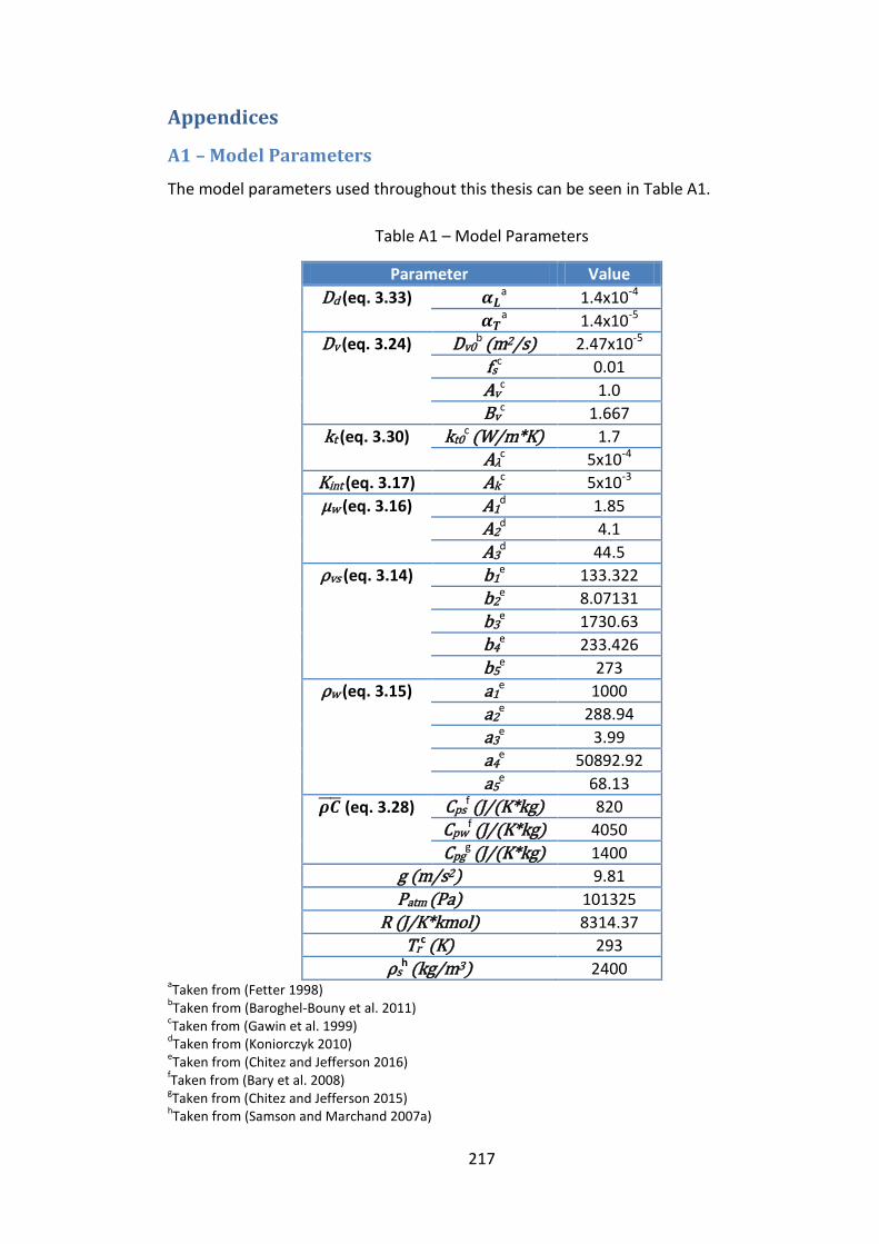
217
Appendices
A1 – Model Parameters
The model parameters used throughout this thesis can be seen in Table A1.
Table A1 – Model Parameters
Parameter Value
Dd (eq. 3.33) a 1.4x10⁻⁴
a 1.4x10⁻⁵
Dv (eq. 3.24) Dv0b
(m2/s) 2.47x10⁻⁵
fsc 0.01
Avc 1.0
Bvc 1.667
kt (eq. 3.30) kt0c (W/m*K) 1.7
Aλc 5x10⁻⁴
Kint (eq. 3.17) Akc 5x10⁻³
μw (eq. 3.16) A1d 1.85
A2d 4.1
A3d 44.5
ρvs (eq. 3.14) b1e 133.322
b2e 8.07131
b3e 1730.63
b4e 233.426
b5e 273
ρw (eq. 3.15) a1e 1000
a2e 288.94
a3e 3.99
a4e 50892.92
a5e 68.13
(eq. 3.28) Cpsf (J/(K*kg) 820
Cpwf (J/(K*kg) 4050
Cpgg
(J/(K*kg) 1400
g (m/s2) 9.81
Patm (Pa) 101325
R (J/K*kmol) 8314.37
Trc (K) 293
ρsh
(kg/m3) 2400 aTaken from (Fetter 1998)
bTaken from (Baroghel-Bouny et al. 2011)
cTaken from (Gawin et al. 1999)
dTaken from (Koniorczyk 2010)
eTaken from (Chitez and Jefferson 2016)
fTaken from (Bary et al. 2008)
gTaken from (Chitez and Jefferson 2015)
hTaken from (Samson and Marchand 2007a)
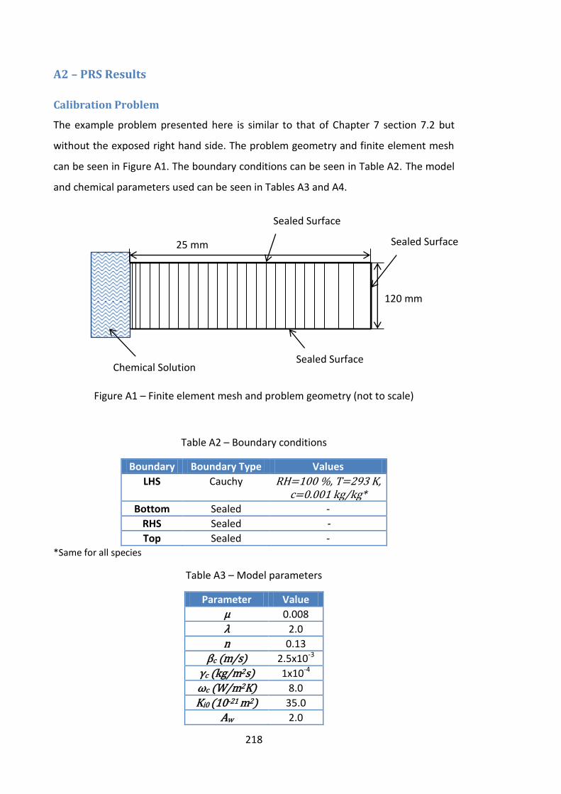
218
A2 – PRS Results
Calibration Problem
The example problem presented here is similar to that of Chapter 7 section 7.2 but
without the exposed right hand side. The problem geometry and finite element mesh
can be seen in Figure A1. The boundary conditions can be seen in Table A2. The model
and chemical parameters used can be seen in Tables A3 and A4.
Figure A1 – Finite element mesh and problem geometry (not to scale)
Table A2 – Boundary conditions
Boundary Boundary Type Values
LHS Cauchy RH=100 %, T=293 K, c=0.001 kg/kg*
Bottom Sealed -
RHS Sealed - Top Sealed -
*Same for all species
Table A3 – Model parameters
Parameter Value
μ 0.008
λ 2.0
n 0.13
βc (m/s) 2.5x10⁻³
γc (kg/m2s) 1x10⁻⁴
ωc (W/m2K) 8.0
Ki0 (10-21 m2) 35.0
Aw 2.0
25 mm
120 mm
Chemical Solution
Sealed Surface
Sealed Surface
Sealed Surface

219
Table A4 – Chemical parameters
Species Dmol
(10-10 m2/s)
Species (cont’d)
Dmol
(10-10 m2/s)
1 0.25 9 6
2 0.5 10 7
3 1 11 8
4 1.5 12 9
5 2 13 10
6 3 14 12
7 4 15 14
8 5 16 16
Non-reactive Diffusion
The first case considered the above boundary conditions with no chemical reactions.
The profiles as predicted by the full model and PRS 1-3 can be seen in Figures A2, A3 &
A4.
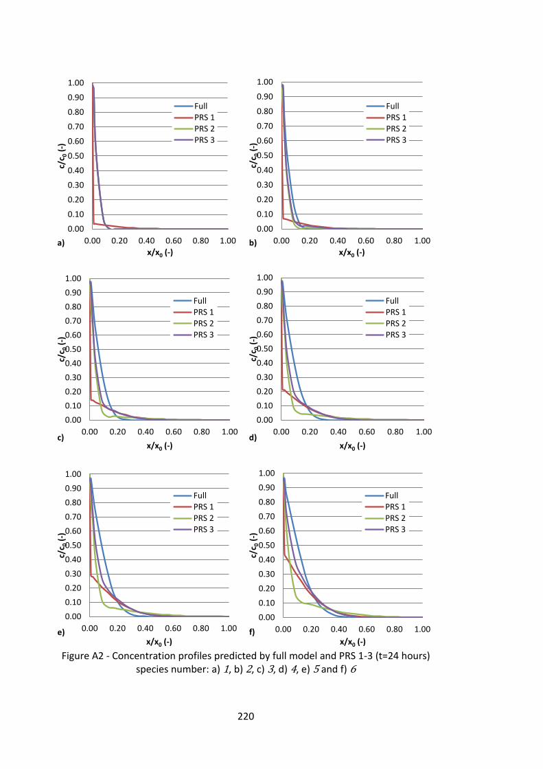
220
Figure A2 - Concentration profiles predicted by full model and PRS 1-3 (t=24 hours)
species number: a) 1, b) 2, c) 3, d) 4, e) 5 and f) 6
0.00
0.10
0.20
0.30
0.40
0.50
0.60
0.70
0.80
0.90
1.00
0.00 0.20 0.40 0.60 0.80 1.00
c/c 0
(-)
x/x0 (-) a)
FullPRS 1PRS 2PRS 3
0.00
0.10
0.20
0.30
0.40
0.50
0.60
0.70
0.80
0.90
1.00
0.00 0.20 0.40 0.60 0.80 1.00
c/c 0
(-)
x/x0 (-)
b)
FullPRS 1PRS 2PRS 3
0.00
0.10
0.20
0.30
0.40
0.50
0.60
0.70
0.80
0.90
1.00
0.00 0.20 0.40 0.60 0.80 1.00
c/c 0
(-)
x/x0 (-) c)
FullPRS 1PRS 2PRS 3
0.00
0.10
0.20
0.30
0.40
0.50
0.60
0.70
0.80
0.90
1.00
0.00 0.20 0.40 0.60 0.80 1.00
c/c 0
(-)
x/x0 (-) d)
FullPRS 1PRS 2PRS 3
0.00
0.10
0.20
0.30
0.40
0.50
0.60
0.70
0.80
0.90
1.00
0.00 0.20 0.40 0.60 0.80 1.00
c/c 0
(-)
x/x0 (-) e)
FullPRS 1PRS 2PRS 3
0.00
0.10
0.20
0.30
0.40
0.50
0.60
0.70
0.80
0.90
1.00
0.00 0.20 0.40 0.60 0.80 1.00
c/c 0
(-)
x/x0 (-) f)
FullPRS 1PRS 2PRS 3

221
Figure A3 - Concentration profiles predicted by full model and PRS 1-3 (t=24 hours)
species number: a) 7, b) 8, c) 9, d) 10, e) 11 and f) 12
0.00
0.10
0.20
0.30
0.40
0.50
0.60
0.70
0.80
0.90
1.00
0.00 0.20 0.40 0.60 0.80 1.00
c/c 0
(-)
x/x0 (-) a)
FullPRS 1PRS 2PRS 3
0.00
0.10
0.20
0.30
0.40
0.50
0.60
0.70
0.80
0.90
1.00
0.00 0.20 0.40 0.60 0.80 1.00
c/c 0
(-)
x/x0 (-) b)
FullPRS 1PRS 2PRS 3
0.00
0.10
0.20
0.30
0.40
0.50
0.60
0.70
0.80
0.90
1.00
0.00 0.20 0.40 0.60 0.80 1.00
c/c 0
(-)
x/x0 (-) c)
FullPRS 1PRS 2PRS 3
0.00
0.10
0.20
0.30
0.40
0.50
0.60
0.70
0.80
0.90
1.00
0.00 0.20 0.40 0.60 0.80 1.00
c/c 0
(-)
x/x0 (-) d)
FullPRS 1PRS 2PRS 3
0.00
0.10
0.20
0.30
0.40
0.50
0.60
0.70
0.80
0.90
1.00
0.00 0.20 0.40 0.60 0.80 1.00
c/c 0
(-)
x/x0 (-) e)
FullPRS 1PRS 2PRS 3
0.00
0.10
0.20
0.30
0.40
0.50
0.60
0.70
0.80
0.90
1.00
0.00 0.20 0.40 0.60 0.80 1.00
c/c 0
(-)
x/x0 (-) f)
FullPRS 1PRS 2PRS 3
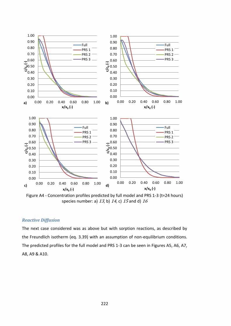
222
Figure A4 - Concentration profiles predicted by full model and PRS 1-3 (t=24 hours)
species number: a) 13, b) 14, c) 15 and d) 16
Reactive Diffusion
The next case considered was as above but with sorption reactions, as described by
the Freundlich isotherm (eq. 3.39) with an assumption of non-equilibrium conditions.
The predicted profiles for the full model and PRS 1-3 can be seen in Figures A5, A6, A7,
A8, A9 & A10.
0.00
0.10
0.20
0.30
0.40
0.50
0.60
0.70
0.80
0.90
1.00
0.00 0.20 0.40 0.60 0.80 1.00
c/c 0
(-)
x/x0 (-) a)
FullPRS 1PRS 2PRS 3
0.00
0.10
0.20
0.30
0.40
0.50
0.60
0.70
0.80
0.90
1.00
0.00 0.20 0.40 0.60 0.80 1.00c/
c 0 (
-)
x/x0 (-) b)
FullPRS 1PRS 2PRS 3
0.00
0.10
0.20
0.30
0.40
0.50
0.60
0.70
0.80
0.90
1.00
0.00 0.20 0.40 0.60 0.80 1.00
c/c 0
(-)
x/x0 (-) c)
FullPRS 1PRS 2PRS 3
0.00
0.10
0.20
0.30
0.40
0.50
0.60
0.70
0.80
0.90
1.00
0.00 0.20 0.40 0.60 0.80 1.00
c/c 0
(-)
x/x0 (-) d)
FullPRS 1PRS 2PRS 3
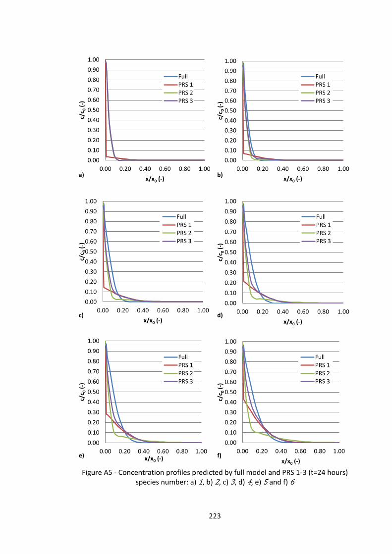
223
Figure A5 - Concentration profiles predicted by full model and PRS 1-3 (t=24 hours)
species number: a) 1, b) 2, c) 3, d) 4, e) 5 and f) 6
0.00
0.10
0.20
0.30
0.40
0.50
0.60
0.70
0.80
0.90
1.00
0.00 0.20 0.40 0.60 0.80 1.00
c/c 0
(-)
x/x0 (-) a)
FullPRS 1PRS 2PRS 3
0.00
0.10
0.20
0.30
0.40
0.50
0.60
0.70
0.80
0.90
1.00
0.00 0.20 0.40 0.60 0.80 1.00
c/c 0
(-)
x/x0 (-) b)
FullPRS 1PRS 2PRS 3
0.00
0.10
0.20
0.30
0.40
0.50
0.60
0.70
0.80
0.90
1.00
0.00 0.20 0.40 0.60 0.80 1.00
c/c 0
(-)
x/x0 (-) c)
FullPRS 1PRS 2PRS 3
0.00
0.10
0.20
0.30
0.40
0.50
0.60
0.70
0.80
0.90
1.00
0.00 0.20 0.40 0.60 0.80 1.00
c/c 0
(-)
x/x0 (-) d)
FullPRS 1PRS 2PRS 3
0.00
0.10
0.20
0.30
0.40
0.50
0.60
0.70
0.80
0.90
1.00
0.00 0.20 0.40 0.60 0.80 1.00
c/c 0
(-)
x/x0 (-) e)
FullPRS 1PRS 2PRS 3
0.00
0.10
0.20
0.30
0.40
0.50
0.60
0.70
0.80
0.90
1.00
0.00 0.20 0.40 0.60 0.80 1.00
c/c 0
(-)
x/x0 (-) f)
FullPRS 1PRS 2PRS 3

224
Figure A6 - Concentration profiles predicted by full model and PRS 1-3 (t=24 hours)
species number: a) 7, b) 8, c) 9, d) 10, e) 11 and f) 12
0.00
0.10
0.20
0.30
0.40
0.50
0.60
0.70
0.80
0.90
1.00
0.00 0.20 0.40 0.60 0.80 1.00
c/c 0
(-)
x/x0 (-) a)
FullPRS 1PRS 2PRS 3
0.00
0.10
0.20
0.30
0.40
0.50
0.60
0.70
0.80
0.90
1.00
0.00 0.20 0.40 0.60 0.80 1.00
c/c 0
(-)
x/x0 (-)
b)
FullPRS 1PRS 2PRS 3
0.00
0.10
0.20
0.30
0.40
0.50
0.60
0.70
0.80
0.90
1.00
0.00 0.20 0.40 0.60 0.80 1.00
c/c 0
(-)
x/x0 (-) c)
FullPRS 1PRS 2PRS 3
0.00
0.10
0.20
0.30
0.40
0.50
0.60
0.70
0.80
0.90
1.00
0.00 0.20 0.40 0.60 0.80 1.00
c/c 0
(-)
x/x0 (-) d)
FullPRS 1PRS 2PRS 3
0.00
0.10
0.20
0.30
0.40
0.50
0.60
0.70
0.80
0.90
1.00
0.00 0.20 0.40 0.60 0.80 1.00
c/c 0
(-)
x/x0 (-) e)
FullPRS 1PRS 2PRS 3
0.00
0.10
0.20
0.30
0.40
0.50
0.60
0.70
0.80
0.90
1.00
0.00 0.20 0.40 0.60 0.80 1.00
c/c 0
(-)
x/x0 (-) f)
FullPRS 1PRS 2PRS 3
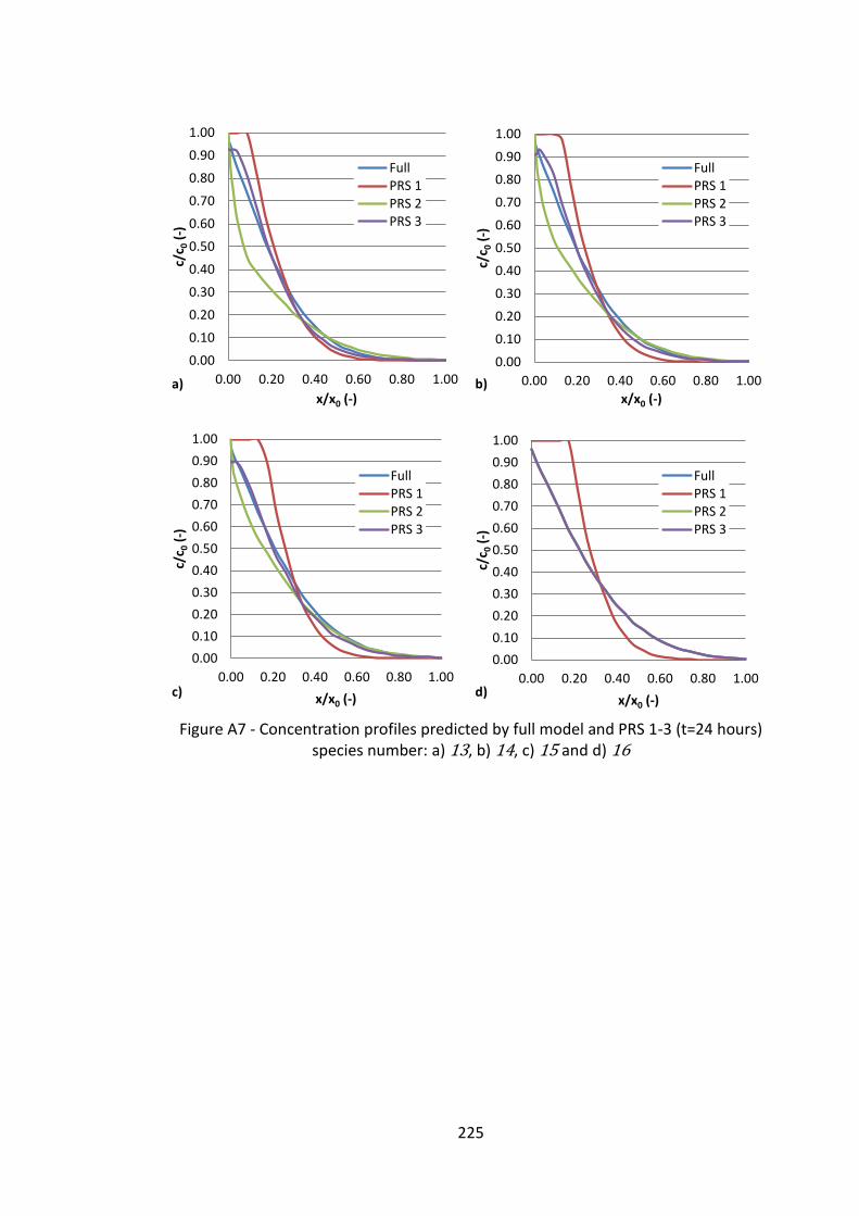
225
Figure A7 - Concentration profiles predicted by full model and PRS 1-3 (t=24 hours)
species number: a) 13, b) 14, c) 15 and d) 16
0.00
0.10
0.20
0.30
0.40
0.50
0.60
0.70
0.80
0.90
1.00
0.00 0.20 0.40 0.60 0.80 1.00
c/c 0
(-)
x/x0 (-) a)
FullPRS 1PRS 2PRS 3
0.00
0.10
0.20
0.30
0.40
0.50
0.60
0.70
0.80
0.90
1.00
0.00 0.20 0.40 0.60 0.80 1.00
c/c 0
(-)
x/x0 (-) b)
FullPRS 1PRS 2PRS 3
0.00
0.10
0.20
0.30
0.40
0.50
0.60
0.70
0.80
0.90
1.00
0.00 0.20 0.40 0.60 0.80 1.00
c/c 0
(-)
x/x0 (-) c)
FullPRS 1PRS 2PRS 3
0.00
0.10
0.20
0.30
0.40
0.50
0.60
0.70
0.80
0.90
1.00
0.00 0.20 0.40 0.60 0.80 1.00
c/c 0
(-)
x/x0 (-) d)
FullPRS 1PRS 2PRS 3
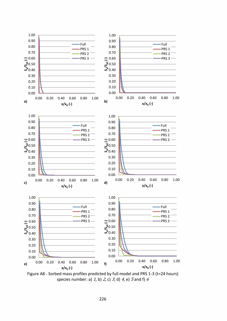
226
Figure A8 - Sorbed mass profiles predicted by full model and PRS 1-3 (t=24 hours)
species number: a) 1, b) 2, c) 3, d) 4, e) 5 and f) 6
0.00
0.10
0.20
0.30
0.40
0.50
0.60
0.70
0.80
0.90
1.00
0.00 0.20 0.40 0.60 0.80 1.00
S p/S
p0
(-)
x/x0 (-) a)
FullPRS 1PRS 2PRS 3
0.00
0.10
0.20
0.30
0.40
0.50
0.60
0.70
0.80
0.90
1.00
0.00 0.20 0.40 0.60 0.80 1.00
S p/S
p0
(-)
x/x0 (-) b)
FullPRS 1PRS 2PRS 3
0.00
0.10
0.20
0.30
0.40
0.50
0.60
0.70
0.80
0.90
1.00
0.00 0.20 0.40 0.60 0.80 1.00
S p/S
p0
(-)
x/x0 (-) c)
FullPRS 1PRS 2PRS 3
0.00
0.10
0.20
0.30
0.40
0.50
0.60
0.70
0.80
0.90
1.00
0.00 0.20 0.40 0.60 0.80 1.00
S p/S
p0
(-)
x/x0 (-) d)
FullPRS 1PRS 2PRS 3
0.00
0.10
0.20
0.30
0.40
0.50
0.60
0.70
0.80
0.90
1.00
0.00 0.20 0.40 0.60 0.80 1.00
S p/S
p0
(-)
x/x0 (-) e)
FullPRS 1PRS 2PRS 3
0.00
0.10
0.20
0.30
0.40
0.50
0.60
0.70
0.80
0.90
1.00
0.00 0.20 0.40 0.60 0.80 1.00
S p/S
p0
(-)
x/x0 (-) f)
FullPRS 1PRS 2PRS 3

227
Figure A9 - Sorbed mass profiles predicted by full model and PRS 1-3 (t=24 hours)
species number: a) 7, b) 8, c) 9, d) 10, e) 11 and f) 12
0.00
0.10
0.20
0.30
0.40
0.50
0.60
0.70
0.80
0.90
1.00
0.00 0.20 0.40 0.60 0.80 1.00
S p/S
p0
(-)
x/x0 (-) a)
FullPRS 1PRS 2PRS 3
0.00
0.10
0.20
0.30
0.40
0.50
0.60
0.70
0.80
0.90
1.00
0.00 0.20 0.40 0.60 0.80 1.00
S p/S
p0 (
-)
x/x0 (-) b)
FullPRS 1PRS 2PRS 3
0.00
0.10
0.20
0.30
0.40
0.50
0.60
0.70
0.80
0.90
1.00
0.00 0.20 0.40 0.60 0.80 1.00
S p/S
p0 (
-)
x/x0 (-) c)
FullPRS 1PRS 2PRS 3
0.00
0.10
0.20
0.30
0.40
0.50
0.60
0.70
0.80
0.90
1.00
0.00 0.20 0.40 0.60 0.80 1.00
S p/S
p0 (
-)
x/x0 (-) d)
FullPRS 1PRS 2PRS 3
0.00
0.10
0.20
0.30
0.40
0.50
0.60
0.70
0.80
0.90
1.00
0.00 0.20 0.40 0.60 0.80 1.00
S p/S
p0
(-)
x/x0 (-) e)
FullPRS 1PRS 2PRS 3
0.00
0.10
0.20
0.30
0.40
0.50
0.60
0.70
0.80
0.90
1.00
0.00 0.20 0.40 0.60 0.80 1.00
S p/S
p0
(-)
x/x0 (-) f)
FullPRS 1PRS 2PRS 3
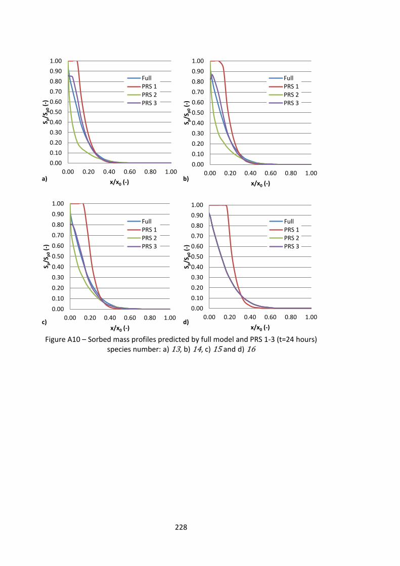
228
Figure A10 – Sorbed mass profiles predicted by full model and PRS 1-3 (t=24 hours)
species number: a) 13, b) 14, c) 15 and d) 16
0.00
0.10
0.20
0.30
0.40
0.50
0.60
0.70
0.80
0.90
1.00
0.00 0.20 0.40 0.60 0.80 1.00
S p/S
p0
(-)
x/x0 (-) a)
FullPRS 1PRS 2PRS 3
0.00
0.10
0.20
0.30
0.40
0.50
0.60
0.70
0.80
0.90
1.00
0.00 0.20 0.40 0.60 0.80 1.00
S p/S
p0 (
-)
x/x0 (-) b)
FullPRS 1PRS 2PRS 3
0.00
0.10
0.20
0.30
0.40
0.50
0.60
0.70
0.80
0.90
1.00
0.00 0.20 0.40 0.60 0.80 1.00
S p/S
p0
(-)
x/x0 (-) c)
FullPRS 1PRS 2PRS 3
0.00
0.10
0.20
0.30
0.40
0.50
0.60
0.70
0.80
0.90
1.00
0.00 0.20 0.40 0.60 0.80 1.00
S p/S
p0
(-)
x/x0 (-) d)
FullPRS 1PRS 2PRS 3
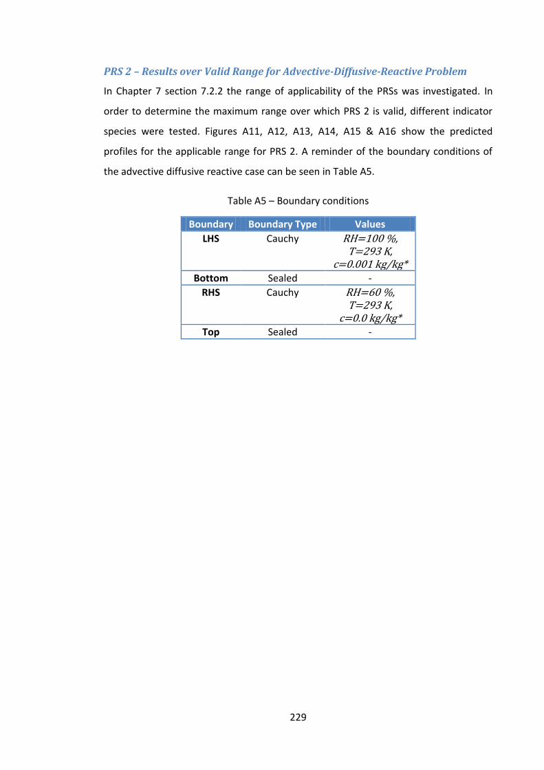
229
PRS 2 – Results over Valid Range for Advective-Diffusive-Reactive Problem
In Chapter 7 section 7.2.2 the range of applicability of the PRSs was investigated. In
order to determine the maximum range over which PRS 2 is valid, different indicator
species were tested. Figures A11, A12, A13, A14, A15 & A16 show the predicted
profiles for the applicable range for PRS 2. A reminder of the boundary conditions of
the advective diffusive reactive case can be seen in Table A5.
Table A5 – Boundary conditions
Boundary Boundary Type Values
LHS Cauchy RH=100 %, T=293 K,
c=0.001 kg/kg* Bottom Sealed -
RHS Cauchy RH=60 %, T=293 K,
c=0.0 kg/kg* Top Sealed -
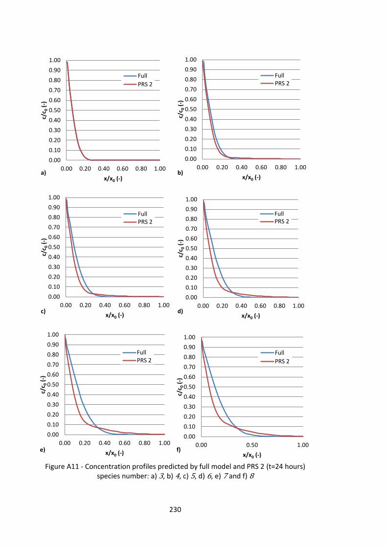
230
Figure A11 - Concentration profiles predicted by full model and PRS 2 (t=24 hours)
species number: a) 3, b) 4, c) 5, d) 6, e) 7 and f) 8
0.00
0.10
0.20
0.30
0.40
0.50
0.60
0.70
0.80
0.90
1.00
0.00 0.20 0.40 0.60 0.80 1.00
c/c 0
(-)
x/x0 (-) a)
Full
PRS 2
0.00
0.10
0.20
0.30
0.40
0.50
0.60
0.70
0.80
0.90
1.00
0.00 0.20 0.40 0.60 0.80 1.00
c/c 0
(-)
x/x0 (-)
b)
FullPRS 2
0.00
0.10
0.20
0.30
0.40
0.50
0.60
0.70
0.80
0.90
1.00
0.00 0.20 0.40 0.60 0.80 1.00
c/c 0
(-)
x/x0 (-) c)
FullPRS 2
0.00
0.10
0.20
0.30
0.40
0.50
0.60
0.70
0.80
0.90
1.00
0.00 0.20 0.40 0.60 0.80 1.00
c/c 0
(-)
x/x0 (-) d)
FullPRS 2
0.00
0.10
0.20
0.30
0.40
0.50
0.60
0.70
0.80
0.90
1.00
0.00 0.20 0.40 0.60 0.80 1.00
c/c 0
(-)
x/x0 (-) e)
FullPRS 2
0.00
0.10
0.20
0.30
0.40
0.50
0.60
0.70
0.80
0.90
1.00
0.00 0.50 1.00
c/c 0
(-)
x/x0 (-) f)
Full
PRS 2
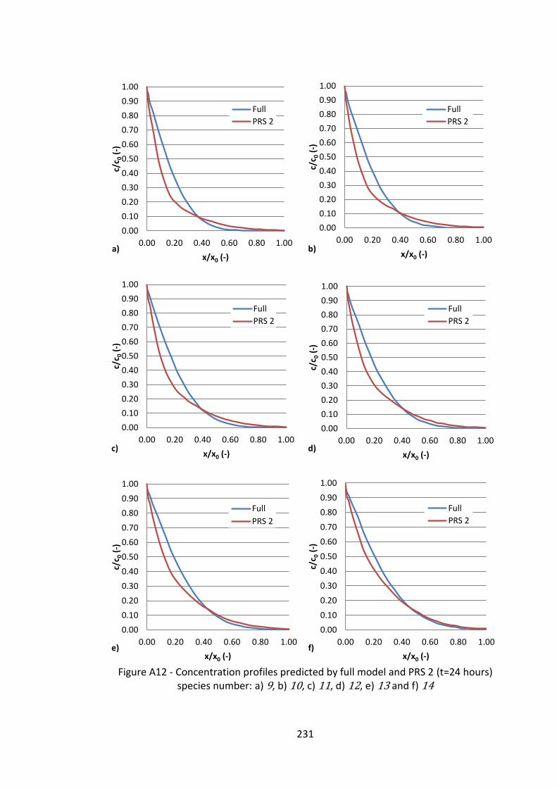
231
Figure A12 - Concentration profiles predicted by full model and PRS 2 (t=24 hours)
species number: a) 9, b) 10, c) 11, d) 12, e) 13 and f) 14
0.00
0.10
0.20
0.30
0.40
0.50
0.60
0.70
0.80
0.90
1.00
0.00 0.20 0.40 0.60 0.80 1.00
c/c 0
(-)
x/x0 (-) a)
Full
PRS 2
0.00
0.10
0.20
0.30
0.40
0.50
0.60
0.70
0.80
0.90
1.00
0.00 0.20 0.40 0.60 0.80 1.00
c/c 0
(-)
x/x0 (-) b)
Full
PRS 2
0.00
0.10
0.20
0.30
0.40
0.50
0.60
0.70
0.80
0.90
1.00
0.00 0.20 0.40 0.60 0.80 1.00
c/c 0
(-)
x/x0 (-) c)
Full
PRS 2
0.00
0.10
0.20
0.30
0.40
0.50
0.60
0.70
0.80
0.90
1.00
0.00 0.20 0.40 0.60 0.80 1.00
c/c 0
(-)
x/x0 (-) d)
Full
PRS 2
0.00
0.10
0.20
0.30
0.40
0.50
0.60
0.70
0.80
0.90
1.00
0.00 0.20 0.40 0.60 0.80 1.00
c/c 0
(-)
x/x0 (-) e)
Full
PRS 2
0.00
0.10
0.20
0.30
0.40
0.50
0.60
0.70
0.80
0.90
1.00
0.00 0.20 0.40 0.60 0.80 1.00
c/c 0
(-)
x/x0 (-) f)
Full
PRS 2
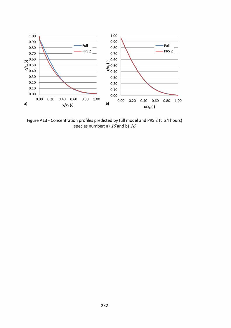
232
Figure A13 - Concentration profiles predicted by full model and PRS 2 (t=24 hours) species number: a) 15 and b) 16
0.00
0.10
0.20
0.30
0.40
0.50
0.60
0.70
0.80
0.90
1.00
0.00 0.20 0.40 0.60 0.80 1.00
c/c 0
(-)
x/x0 (-) a)
Full
PRS 2
0.00
0.10
0.20
0.30
0.40
0.50
0.60
0.70
0.80
0.90
1.00
0.00 0.20 0.40 0.60 0.80 1.00
c/c 0
(-)
x/x0 (-)
b)
Full
PRS 2
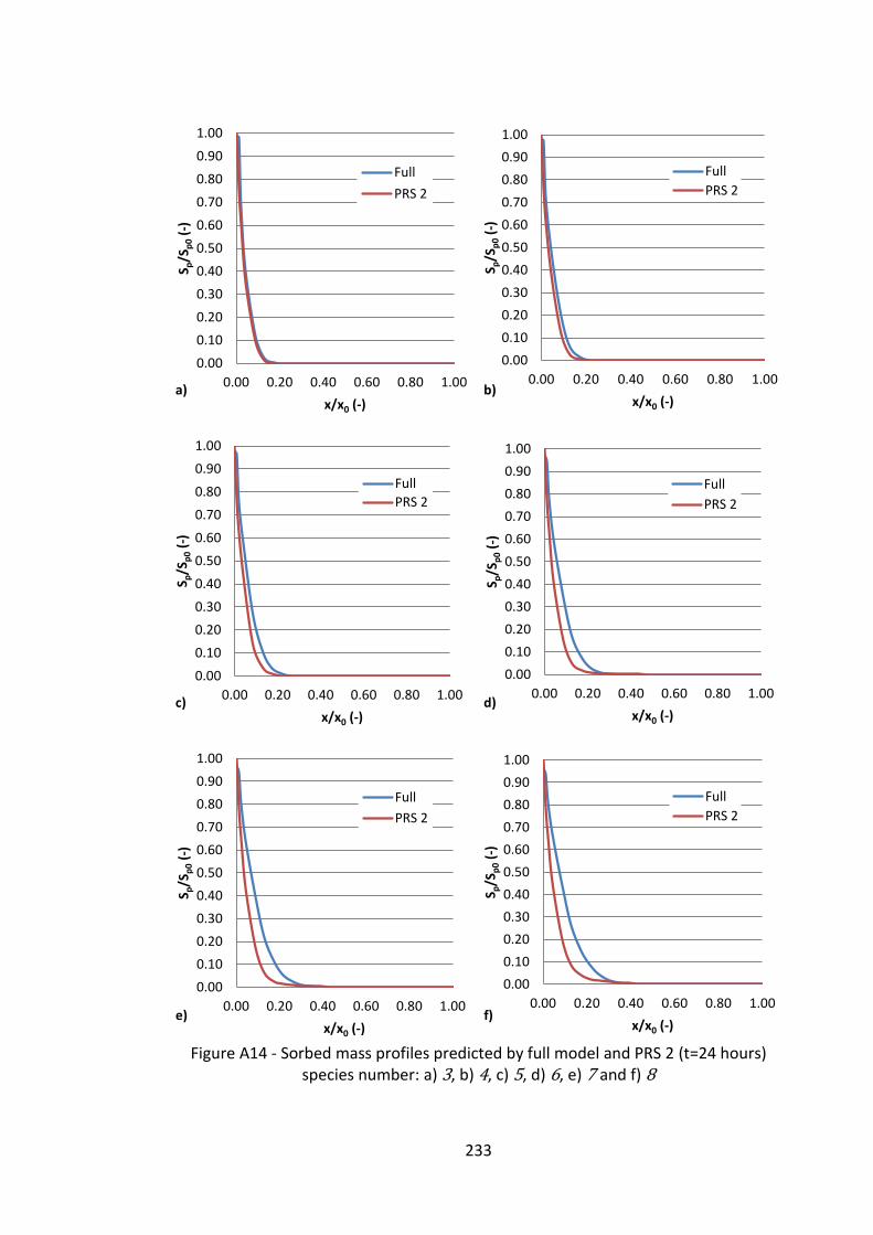
233
Figure A14 - Sorbed mass profiles predicted by full model and PRS 2 (t=24 hours)
species number: a) 3, b) 4, c) 5, d) 6, e) 7 and f) 8
0.00
0.10
0.20
0.30
0.40
0.50
0.60
0.70
0.80
0.90
1.00
0.00 0.20 0.40 0.60 0.80 1.00
S p/S
p0
(-)
x/x0 (-) a)
Full
PRS 2
0.00
0.10
0.20
0.30
0.40
0.50
0.60
0.70
0.80
0.90
1.00
0.00 0.20 0.40 0.60 0.80 1.00
S p/S
p0
(-)
x/x0 (-) b)
Full
PRS 2
0.00
0.10
0.20
0.30
0.40
0.50
0.60
0.70
0.80
0.90
1.00
0.00 0.20 0.40 0.60 0.80 1.00
S p/S
p0
(-)
x/x0 (-) c)
Full
PRS 2
0.00
0.10
0.20
0.30
0.40
0.50
0.60
0.70
0.80
0.90
1.00
0.00 0.20 0.40 0.60 0.80 1.00
S p/S
p0
(-)
x/x0 (-) d)
Full
PRS 2
0.00
0.10
0.20
0.30
0.40
0.50
0.60
0.70
0.80
0.90
1.00
0.00 0.20 0.40 0.60 0.80 1.00
S p/S
p0
(-)
x/x0 (-) e)
Full
PRS 2
0.00
0.10
0.20
0.30
0.40
0.50
0.60
0.70
0.80
0.90
1.00
0.00 0.20 0.40 0.60 0.80 1.00
S p/S
p0
(-)
x/x0 (-) f)
Full
PRS 2
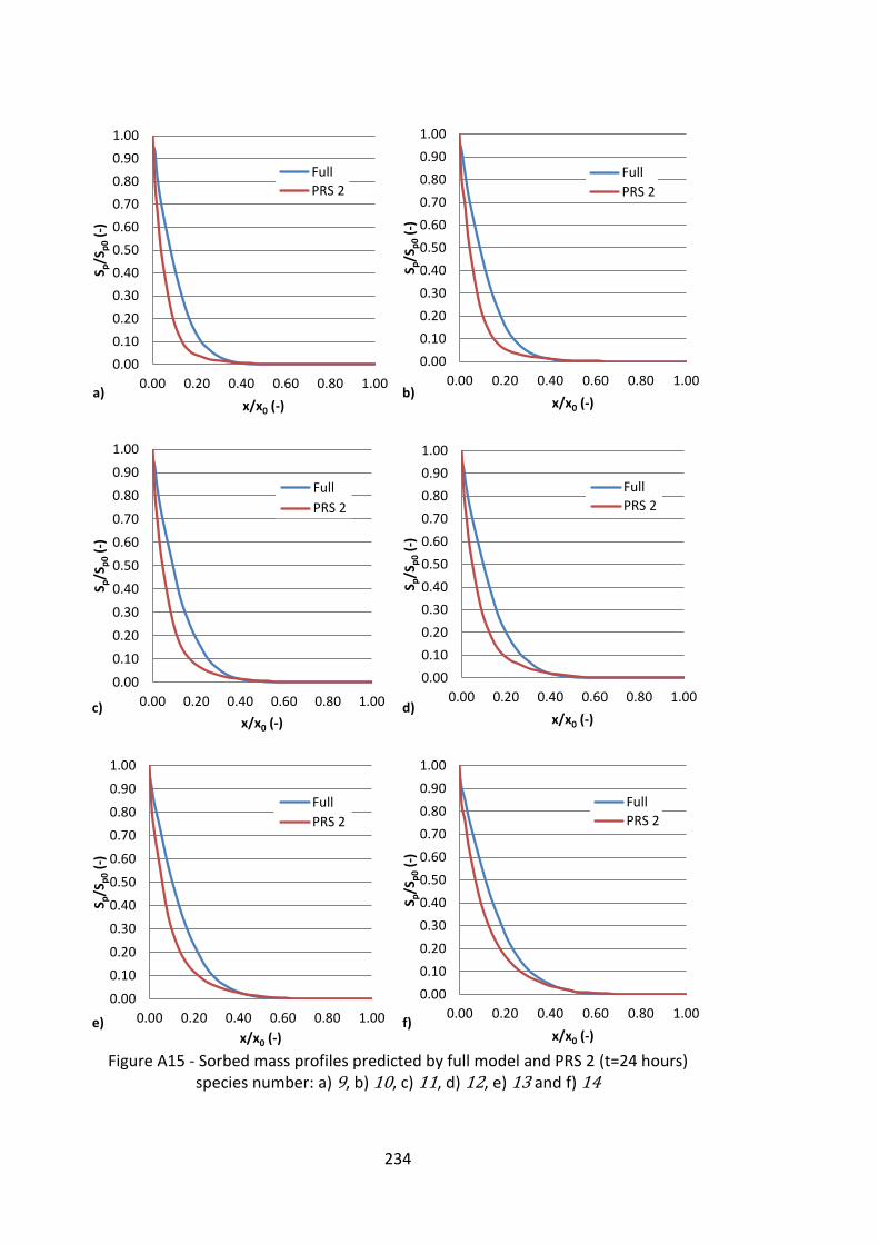
234
Figure A15 - Sorbed mass profiles predicted by full model and PRS 2 (t=24 hours)
species number: a) 9, b) 10, c) 11, d) 12, e) 13 and f) 14
0.00
0.10
0.20
0.30
0.40
0.50
0.60
0.70
0.80
0.90
1.00
0.00 0.20 0.40 0.60 0.80 1.00
S p/S
p0
(-)
x/x0 (-) a)
Full
PRS 2
0.00
0.10
0.20
0.30
0.40
0.50
0.60
0.70
0.80
0.90
1.00
0.00 0.20 0.40 0.60 0.80 1.00
S p/S
p0 (
-)
x/x0 (-) b)
Full
PRS 2
0.00
0.10
0.20
0.30
0.40
0.50
0.60
0.70
0.80
0.90
1.00
0.00 0.20 0.40 0.60 0.80 1.00
S p/S
p0
(-)
x/x0 (-) c)
Full
PRS 2
0.00
0.10
0.20
0.30
0.40
0.50
0.60
0.70
0.80
0.90
1.00
0.00 0.20 0.40 0.60 0.80 1.00
S p/S
p0
(-)
x/x0 (-) d)
Full
PRS 2
0.00
0.10
0.20
0.30
0.40
0.50
0.60
0.70
0.80
0.90
1.00
0.00 0.20 0.40 0.60 0.80 1.00
S p/S
p0
(-)
x/x0 (-) e)
Full
PRS 2
0.00
0.10
0.20
0.30
0.40
0.50
0.60
0.70
0.80
0.90
1.00
0.00 0.20 0.40 0.60 0.80 1.00
S p/S
p0
(-)
x/x0 (-) f)
Full
PRS 2
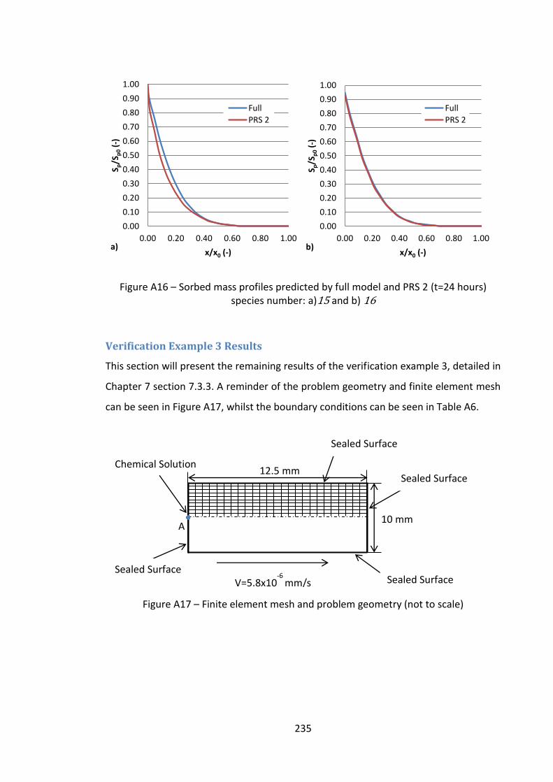
235
Figure A16 – Sorbed mass profiles predicted by full model and PRS 2 (t=24 hours) species number: a)15 and b) 16
Verification Example 3 Results
This section will present the remaining results of the verification example 3, detailed in
Chapter 7 section 7.3.3. A reminder of the problem geometry and finite element mesh
can be seen in Figure A17, whilst the boundary conditions can be seen in Table A6.
Figure A17 – Finite element mesh and problem geometry (not to scale)
0.00
0.10
0.20
0.30
0.40
0.50
0.60
0.70
0.80
0.90
1.00
0.00 0.20 0.40 0.60 0.80 1.00
S p/S
p0 (
-)
x/x0 (-) a)
Full
PRS 2
0.00
0.10
0.20
0.30
0.40
0.50
0.60
0.70
0.80
0.90
1.00
0.00 0.20 0.40 0.60 0.80 1.00
S p/S
p0 (
-)
x/x0 (-) b)
Full
PRS 2
12.5 mm
10 mm A
V=5.8x10⁻⁶
mm/s
Chemical Solution
Sealed Surface
Sealed Surface
Sealed Surface Sealed Surface
236
Table A6 – Boundary conditions
Boundary Boundary Type Values
LHS Cauchy RH=100 %, T=293 K, c*
Bottom q=0 -
RHS Sealed -
Top Sealed - *See chemical parameters table
The model and chemical parameters used in the model can be seen in Table A7 and
Table A8 respectively.
Table A7 – Model parameters
Parameter Value
n 0.3
γc (kg/m2s) 1e-4
ωc (W/m2K) 8.0
Table A8 – Chemical parameters
Species Initial Conc. (kg/kg)
Boundary Conc.
(kg/kg)
Dmol
(10-9 m2/s) Eq. ka
(10-7) kd
(10-8) λ
H+ 0.000028 0.00005 9.311 r1 2.6 29.6 0.61
Ca2+ 0.0003164 0.00048 0.792 r2 0.6 8.67 0.2
Mg2+ 0.00102303 0.001944 0.706 r3 1.4 9.0 0.07
HCO3- 0.00061 0.0000305 1.185 r4 2.8 2.0 0.11
Al3+ 0.000837 0.00135 0.541 r5 2.1 6.0 0.43
SO42 0.016896 0.024 1.065 r6 0.425 74.0 0.35
Fe3+ 0.00199206 0.00279 0.604
K+ 0.00006123 0.000078 1.957
Cl- 0.0010295 0.001775 2.032
Na+ 0.0018515 0.000345 1.334
SiO2 0.015 - -
The concentration profiles along the y axis -obtained by taking a cut along line A-A
seen in Figure A18- as predicted by the full model and PRS 3 can be seen in Figures A19
& A20, whilst the sorbed mass profiles can be seen in Figures A21 & A22. Finally the
correlation plots can be seen in Figure A23.
237
Figure A18 - Problem geometry and cut lines
Figure A19 - Concentration profiles (taken along cut line A-A) predicted by the full
model and PRS 3 (t=10 hours) a) H+, b) Ca2+, c) Mg2+ and d) HCO32-
0.00E+00
5.00E-06
1.00E-05
1.50E-05
2.00E-05
2.50E-05
3.00E-05
3.50E-05
4.00E-05
0 0.002 0.004
Co
nce
ntr
atio
n (
kg/k
g)
Distance from Exposed Face (m) a)
Full
PRS 30.00E+00
5.00E-05
1.00E-04
1.50E-04
2.00E-04
2.50E-04
3.00E-04
3.50E-04
4.00E-04
4.50E-04
5.00E-04
0 0.002 0.004
Co
nce
ntr
atio
n (
kg/k
g)
Distance from Exposed Face (m) b)
Full
PRS 3
0.00E+00
2.00E-04
4.00E-04
6.00E-04
8.00E-04
1.00E-03
1.20E-03
1.40E-03
1.60E-03
1.80E-03
2.00E-03
0 0.002 0.004
Co
nce
ntr
atio
n (
kg/k
g)
Distance from Exposed Face (m) c)
Full
PRS 30.00E+00
1.00E-04
2.00E-04
3.00E-04
4.00E-04
5.00E-04
6.00E-04
7.00E-04
0 0.002 0.004
Co
nce
ntr
atio
n (
kg/k
g)
Distance from Exposed Face (m) d)
Full
PRS 3
12.5 mm
10 mm
A
A
B B
238
Figure A20 - Concentration profiles (taken along cut line A-A) predicted by the full
model and PRS 3 (t=10 hours) a) Al3+, b) SO42-, c) Fe3+, d) K+, e) Cl- and f) Na+
0.00E+00
2.00E-04
4.00E-04
6.00E-04
8.00E-04
1.00E-03
1.20E-03
1.40E-03
0 0.002 0.004
Co
nce
ntr
atio
n (
kg/k
g)
Distance from Exposed Face (m) a)
Full
PRS 30.00E+00
5.00E-03
1.00E-02
1.50E-02
2.00E-02
2.50E-02
0 0.002 0.004
Co
nce
ntr
atio
n (
kg/k
g)
Distance from Exposed Face (m) b)
Full
PRS 3
0.00E+00
5.00E-04
1.00E-03
1.50E-03
2.00E-03
2.50E-03
3.00E-03
0 0.002 0.004
Co
nce
ntr
atio
n (
kg/k
g)
Distance from Exposed Face (m) c)
Full
PRS 30.00E+00
1.00E-05
2.00E-05
3.00E-05
4.00E-05
5.00E-05
6.00E-05
7.00E-05
8.00E-05
0 0.002 0.004
Co
nce
ntr
atio
n (
kg/k
g)
Distance from Exposed Face (m) d)
Full
PRS 3
0.00E+00
2.00E-04
4.00E-04
6.00E-04
8.00E-04
1.00E-03
1.20E-03
1.40E-03
1.60E-03
1.80E-03
0 0.002 0.004
Co
nce
ntr
atio
n (
kg/k
g)
Distance from Exposed Face (m) e)
Full
PRS 30.00E+00
5.00E-04
1.00E-03
1.50E-03
2.00E-03
2.50E-03
0 0.002 0.004
Co
nce
ntr
atio
n (
kg/k
g)
Distance from Exposed Face (m) f)
Full
PRS 3
239
Figure A21 - Solid mass profiles (taken along cut line A-A) predicted by the full model
and PRS 3 (t=10 hours) a) Al(OH)3, b) CaSO4.2H20, c) K0.6Mg0.25Al2.3Si3.5O10(OH)2 and d) Fe(OH)3
0.00E+00
5.00E-07
1.00E-06
1.50E-06
2.00E-06
2.50E-06
3.00E-06
3.50E-06
0 0.002 0.004
Solid
Mas
s (k
g/kg
)
Distance from Exposed Face (m) a)
Full
PRS 30.00E+00
5.00E-07
1.00E-06
1.50E-06
2.00E-06
2.50E-06
0 0.002 0.004
Solid
Mas
s (k
g/kg
)
Distance from Exposed Face (m) b)
Full
PRS 3
0.00E+00
2.00E-05
4.00E-05
6.00E-05
8.00E-05
1.00E-04
1.20E-04
1.40E-04
1.60E-04
0 0.002 0.004
Solid
Mas
s (k
g/kg
)
Distance from Exposed Face (m) c)
Full
PRS 30.00E+00
2.00E-05
4.00E-05
6.00E-05
8.00E-05
1.00E-04
1.20E-04
1.40E-04
1.60E-04
1.80E-04
0 0.002 0.004
Solid
Mas
s (k
g/kg
)
Distance from Exposed Face (m) d)
Full
PRS 3
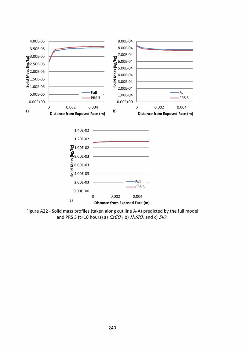
240
Figure A22 - Solid mass profiles (taken along cut line A-A) predicted by the full model
and PRS 3 (t=10 hours) a) CaCO3, b) H4SiO4 and c) SiO2
0.00E+00
5.00E-06
1.00E-05
1.50E-05
2.00E-05
2.50E-05
3.00E-05
3.50E-05
4.00E-05
0 0.002 0.004
Solid
Mas
s (k
g/kg
)
Distance from Exposed Face (m) a)
Full
PRS 30.00E+00
1.00E-04
2.00E-04
3.00E-04
4.00E-04
5.00E-04
6.00E-04
7.00E-04
8.00E-04
9.00E-04
0 0.002 0.004
Solid
Mas
s (k
g/kg
) Distance from Exposed Face (m)
b)
Full
PRS 3
0.00E+00
2.00E-03
4.00E-03
6.00E-03
8.00E-03
1.00E-02
1.20E-02
1.40E-02
0 0.002 0.004
Solid
Mas
s (k
g/kg
)
Distance from Exposed Face (m) c)
Full
PRS 3

241
Figure A23 - Correlation of concentrations and solid mass
0.00
0.10
0.20
0.30
0.40
0.50
0.60
0.70
0.80
0.90
1.00
0.00 0.10 0.20 0.30 0.40 0.50 0.60 0.70 0.80 0.90 1.00
Co
nce
ntr
atio
n P
red
icte
d b
y Fu
ll M
od
el
(-)
Concentration Predicted by PRS 3 (-)
H
Ca
Mg
HCO3
Al
SO4
Fe
K
Cl
Na
y=x
0.00
0.10
0.20
0.30
0.40
0.50
0.60
0.70
0.80
0.90
1.00
0.00 0.10 0.20 0.30 0.40 0.50 0.60 0.70 0.80 0.90 1.00
Solid
Mas
s C
on
c. P
red
icte
d b
y Fu
ll M
od
el (
-)
Solid Mass Conc. Predicted by PRS 3 (-)
Al(OH)3
Gypsum
Illite
Fe(OH)3
CaCO3
H4SiO4
SiO2
y=x


![Thermochemistry [Thermochemical Equations, Enthalpy Change and Standard Enthalpy of Formation]](https://img.pdfslide.net/doc/110x75/557ddcecd8b42a4e358b4995/thermochemistry-thermochemical-equations-enthalpy-change-and-standard-enthalpy-of-formation.jpg)