Embed Size (px)
Citation preview

DOKUZ EYLÜL UNIVERSITY GRADUATE SCHOOL OF NATURAL AND APPLIED SCIENCES
A NUMERICAL STUDY ON THE THERMAL
EXPANSION COEFFICIENTS OF FIBER
REINFORCED COMPOSITE MATERIALS
by
Ziya Haktan KARADENİZ
July, 2005
İZMİR

A NUMERICAL STUDY ON THE THERMAL
EXPANSION COEFFICIENTS OF FIBER
REINFORCED COMPOSITE MATERIALS
A Thesis Submitted to the
Graduate School of Natural and Applied Sciences of Dokuz Eylül University
In Partial Fulfillment of the Requirements for the Degree of
Master of Science in Mechanical Engineering, Energy Program
by
Ziya Haktan KARADENİZ
July, 2005
İZMİR

M.Sc THESIS EXAMINATION RESULT FORM
We have read the thesis entitled “A NUMERICAL STUDY ON THE THERMAL
EXPANSION COEFFICIENTS OF FIBER REINFORCED COMPOSITE
MATERIALS” completed by Ziya Haktan KARADENİZ under supervision of
Assist. Prof. Dr. Dilek KUMLUTAŞ and we certify that in our opinion it is fully
adequate, in scope and in quality, as a thesis for the degree of Master of Science.
Ş
(Jury Member)
Gradua
Assist. Prof. Dr. Dilek KUMLUTA
Supervisor
(Jury Member)
Prof.Dr. Cahit HELVACI Director
te School of Natural and Applied Sciences
ii

ACKNOWLEDGEMENTS
I would like to thank to my supervisor Assist. Prof. Dr. Dilek KUMLUTAŞ for
her guidance, valuable advises, incomparable helps and considerable concern in
carrying out the study.
I would especially like to thank to my family for their helpful encouragement and
valuable support.
Finally, I would like to thank my fiancée for her unconditional friendship,
unlimited patience, moral support and unconditional love.
iii

A NUMERICAL STUDY ON THE THERMAL EXPANSION
COEFFICIENTS OF FIBER REINFORCED COMPOSITE MATERIALS
ABSTRACT
In the present work, the effective CTE of different kinds of fiber reinforced
composites is studied by micromechanical modeling using finite element method. To
determine the both longitudinal and transverse CTEs of composites, three
dimensional steady state analyses were undertaken. Representative unit cell models,
cylinder which is embedded in a cube with unit dimension, having different fiber
volume fractions were produced using finite element program ANSYS. Fibers are
assumed to have a square packing arrangement. To compare the results of finite
element solutions for different types of composites with the results of the analytical
methods and to determine the expansion behavior of different material systems with
respect to fiber content, models having fiber volume fractions from 10% to 80% with
increments of 10% have been composed. Furthermore, comparison between finite
element solutions and experimental results have been made upon the models having
40%, 47%, 48%, 54%, 57%, 63%, 65%, and 68% fiber volume fractions.
Present numerical finite element solution by ANSYS is in excellent agreement
with the analytical solution by Rosen and Hashin and in sufficient agreement with
other analytical solutions. The comparisons of these model predictions with
experimental data show that for some material the agreement is very good, but for
others there is some discrepancy between the experimental results and model
predictions. The reason may be that the fiber-matrix interface bond which was
assumed to be perfect was not really so in the experimental materials. The interface
may either contain interfacial cracks or it might have elastic properties different from
those of matrix and fiber.
Keywords: Coefficient of thermal expansion, fiber reinforced composites, ANSYS,
micromechanical modeling.
iv

LİF KATKILI KOMPOZİT MALZEMELERİN ISIL GENLEŞME
KATSAYILARI ÜZERİNE SAYISAL BİR ÇALIŞMA
ÖZ
Bu çalışmada, farklı türde lif ve matris malzemelerden oluşan kompozit
malzemelerin ısıl genleşme katsayıları önce mevcut analitik yöntemlerle belirlenmiş,
daha sonra kompozit malzemelerin mikro yapıları temsili birim hücreler şeklinde
modellenerek sonlu elemanlar yöntemiyle çözüm yapan ANSYS programı
kullanılarak analizler yapılmıştır. Malzemelerin enine ve boyuna ısıl enleşme
katsayılarını belirleyebilmek için birim kenarlı bir küp içine yerleştirilmiş bir silindir
şeklinde üç boyutlu mikro yapı modelleri oluşturulmuştur. Liflerin matris malzeme
içinde karesel düzende dağıldığı varsayılmıştır.
Lif doğrultusu, miktarı ve türünün malzemenin ısıl genleşme katsayısı üzerindeki
etkilerini incelemek ve analitik yöntemlerle sonlu elemanlar yöntemini
karşılaştırmak için tüm kompozit malzemelerin %10’luk aralıklarla %10 - %80
aralığında hacimsel lif oranına sahip modelleri oluşturulmuştur. Bununla birlikte elde
edilen sonuçları mevcut deney sonuçlarıyla karşılaştırmak için 40%, 47%, 48%,
54%, 57%, 63%, 65% ve 68% hacimsel oranlarında lif içeren modeller
oluşturulmuştur.
Sonlu elemanlar yönteminin Rosen-Hashin yöntemiyle iyi uyum gösterdiği diğer
analitik yöntemlerle de uyumlu olduğu görülmüştür. Deney sonuçları ile en iyi
uyumu sonlu elemanlar yöntemi göstermiştir. Diğer analitik yöntemler ise bazı
malzemeler için iyi sonuçlar verirken bazılarında deney sonuçlarına göre yüksek
sapma göstermişlerdir. Kompozit malzemenin ısıl genleşme katsayısını belirlemek
için sonlu elemanlar yönteminin güvenilir bir yol olduğu görülmüştür.
Anahtar kelimeler: Isıl genleşme katsayısı, lif katkılı kompozitler, ANSYS, mikro
yapı modelleri.
v

CONTENTS
Page
THESIS EXAMINATION RESULT FORM .......................................................ii
ACKNOWLEDGEMENTS ................................................................................ iii
ABSTRACT.........................................................................................................iv
ÖZ .........................................................................................................................v
CONTENTS.........................................................................................................vi
CHAPTER ONE – INTRODUCTION .............................................................1
1.1 Introduction................................................................................................1
CHAPTER TWO – FIBER REINFORCED COMPOSITES.........................7
2.1 Composites.................................................................................................7
2.2 Fiber Reinforced Composites.....................................................................8
2.2.1 Matrix Materials.................................................................................8
2.2.1.1 Polymer Matrix Materials ..........................................................9
2.2.1.2 Metal Matrix Materials ............................................................11
2.2.1.3 Ceramic Matrix Materials ........................................................12
2.2.2 Fibers................................................................................................13
2.2.2.1 Boron Fibers.............................................................................15
2.2.2.2 Carbon Fibers ...........................................................................16
2.2.2.3 Ceramic Fibers .........................................................................18
2.2.2.4 Glass Fibers..............................................................................19
2.2.2.5 Organic Fibers..........................................................................21
2.2.2.5.1 Cellulose Fibers................................................................22
2.2.2.5.2 Oriented Polyethylene Fibers...........................................23
2.2.2.5.3 Aramid Fibers ..................................................................24
2.2.2.6 Whiskers...................................................................................26
vi

CHAPTER THREE – THERMAL EXPANSION BEHAVIOUR OF FIBER
REINFORCED COMPOSITES ................................................................27
3.1 Coefficient of Thermal Expansion (CTE)................................................27
3.2 Factors Affecting the Coefficient of Thermal Expansion ........................28
3.2.1 Fiber Volume ...................................................................................28
3.2.2 Void Volume....................................................................................29
3.2.3 Lay-up Angle ...................................................................................29
3.2.4 Thermal Cycling ..............................................................................30
3.2.5 Temperature Dependence.................................................................30
3.2.6 Moisture Effects ...............................................................................30
3.2.7 Viscoelasticty ...................................................................................31
3.3 Thermal Expansion Measurement Techniques ........................................31
3.3.1 Mechanical Dilatometry...................................................................32
3.3.2 Interferometry ..................................................................................34
3.3.3 Strain Gauges ...................................................................................36
3.4 Theoretical Consideration .......................................................................37
3.4.1 Some of the Existing Theories .........................................................38
3.4.1.1 Law of Mixtures.......................................................................38
3.4.1.2 Equation of Thomas .................................................................39
3.4.1.3 Equation of Van Fo Fy.............................................................40
3.4.1.4 Equation of Cribb.....................................................................40
3.4.1.5 Equation of Schapery ...............................................................41
3.4.1.6 Equation of Chamberlain .........................................................42
3.4.1.7 Equation of Rosen and Hashin.................................................43
3.4.1.8 Equation of Schneider ..............................................................44
3.4.1.9 Equation of Chamis..................................................................45
3.4.1.10 Equation of Sideridis..............................................................45
CHAPTER FOUR – FINITE ELEMENT METHOD...................................48
4.1 Historical Perspective...............................................................................48
4.2 Finite Element Analysis Procedure..........................................................49
vii

4.2.1 Geometry Creation...........................................................................49
4.2.2 Mesh Creation and Element Selection............................................50
4.2.3 Boundary and Loading Conditions ..................................................51
4.2.4 Defining Material Properties...........................................................52
4.2.5 Displaying Results ...........................................................................53
CHAPTER FIVE – MICROMECHANICAL ANALYIS BY ANSYS ........54
5.1 Model Development.................................................................................54
5.2 Mesh Creation ..........................................................................................56
5.3 Material Properties ...................................................................................57
5.4 Boundary Conditions ...............................................................................59
5.5 Solution ....................................................................................................59
CHAPTER SIX – RESULTS AND DISCUSSION ........................................61
REFERENCES..................................................................................................73
viii

CHAPTER ONE
INTRODUCTION
1.1 Introduction
Structural composite materials typically consist of a primary load-carrying (stiff
and strong) material phase, such as fibers, held together by a binder of matrix
material, often an organic polymer. Matrix is soft and weak, and its direct load
bearing is negligible. However, the role of matrix is very important for the structural
integrity of composites; matrix protects fibers from hostile environments and
localizes the effect of broken fibers. In order to achieve particular elastic properties
in preferred directions, continuous fibers are usually employed in structures having
essentially two dimensional characteristics. For convenience of construction, the
fibers in the form of multifilament tows are laid parallel and impregnated with the
matrix resin to form an uncured unidirectional lamina as the basic element of
construction. The final complex structure is then produced by stacking the individual
lamina in an appropriate sequence and orientation, curing under heat and pressure, to
form rigid laminate which possesses the directional characteristics required.
The complexities of composite materials are due to the unknown features such as
chemical compatibility, wettability, adsorption characteristics and stress development
resulting from differences in thermal and moisture expansion, have so far restricted
their complete characterization. Understanding the behavior of composites relative to
the properties of fiber and matrix materials is desirable not only for the practical
purpose of predicting the properties of composites but also for the fundamental
knowledge required in developing new materials.
Linear thermal expansion is the fractional change in length of a body when heated
or cooled through a given temperature range and usually it is given as a coefficient
per unit temperature interval, either as an average over stated range, or as the tangent
to the expansion curve at a given temperature. The longitudinal and transverse
1

2
coefficients of thermal expansion of the orthotropic unidirectional lamina must be
known for design purposes. These composite properties can be experimentally
measured, which can be expensive and time consuming when evaluating many
different material systems, or predicted using the thermal and mechanical properties
of the constituents. Furthermore, as a result of the increasing computer technology,
numerical solutions such as finite element analysis are being used to determine the
thermal expansion coefficients of composite materials. Since polymer matrix
materials typically exhibit thermal expansion coefficients which are much higher
than those of fibers and the fiber may be thermally as well as mechanically
anisotropic, complex stress states are induced in the composite due to temperature
changes.
The problem of relating effective mechanical properties of fiber reinforced
composite materials to constituent properties has received considerable attention.
Many analytical models exist for the prediction of the coefficients of thermal
expansion for unidirectional composites. In the first half of the 20th century the
mathematical complexity of the analysis in the various theories had been ranging
from the simple netting analysis to sophisticated statistical methods. The various
assumptions underlying these theories were not always explicitly stated. In general
they tended to be unrealistic simplifications of the physical state of the materials.
These simplifications resulted in theories which do not have satisfactory correlation
with experimental data. To obtain better theory-experiment correlation, some of the
investigators introduced correction factors. But application of these theories became
a matter of the user’s familiarity and talent, and resulted in a hopeless case of
confusion for the researchers. A critique on theories predicting thermoelastic
properties of fiber reinforced composite materials was presented by Chamis and
Sendeckyj (1968) where they had introduced basic principles of existing theories and
had reviewed individual papers.
A number of articles on thermal expansion of fiber reinforced composites had
appeared during 1960s in Russian literature (Shapery, 1968). In an important paper
by Levin (1967), effective thermal expansion coefficients for two-phase anisotropic

3
composites with isotropic phases were derived using an extension of Hill’s method
(1964). Exact relations were given from which composite thermal expansion
coefficients may be determined if constituent properties and effective composite
moduli are known. In a series of articles by Van Fo Fy (1965, 1966), exact thermal
expansion coefficients for matrices reinforced by doubly periodic array of hollow or
solid circular continuous fibers were developed by means of a detailed stress
analysis.
Another method for calculating upper and lower bounds on thermal expansion
coefficients of isotropic and anisotropic composites with isotropic phases, and some
explicit formulas for volumetric and linear coefficients of thermal expansion was
given by Shapery (1968). In contrast to work by Levin and Van Fo Fy composites
with an arbitrary number of different constituents and arbitrary phase geometry can
be treated by Shapery’s formula. His method employed the complementary and
potential energy principles of thermoelasticity theory in conjunction with a procedure
for minimizing the difference between upper and lower bounds. It was shown that for
some important cases the bounds coincide and therefore yield exact solutions.
Shapery’s formula has been the most useful solution to determine the longitudinal
thermal expansion coefficient afterwards.
An alternative model for transverse thermal expansion of unidirectional
composites was derived by Chamberlain (Rogers et al., 1977), using plane stress
thick walled cylinder equations for the case of transversely isotropic fibers embedded
in an isotropic cylindrical matrix.
Rosen and Hashin (1970) developed relations to determine the upper and lower
bounds on effective thermal expansion coefficients of anisotropic composites having
any number of anisotropic phases using thermoelastic energy principles. The bounds
they found are complicated algebraic expressions but reduction to simpler form is
possible when symmetry of the phases and composite is taken into account. For
isotropic phases, the thermal expansion results reduce to the bounds obtained by
Shapery (1968). When the composite has only two phases, thermal expansion
4
coefficients coincide to give results in the form of unique functions of the elastic
moduli.
Another consideration was made by Sideridis (1994) who developed the model of
the inhomogeneous boundary interphase. He studied the influence of the mode of
variation of boundary’s thermal expansion coefficient, elastic modulus and Poisson’s
ratio versus the polar radius between the fiber and the matrix in the representative
volume element of a unidirectional fiber composite on the overall value of the
composite thermal expansion coefficients. He also made experiments on E-glass-
epoxy composites and showed that for all volume fractions the thermal expansion
values derived from his solutions are similar to both experiments and the respective
values derived from the equations of Shapery and Van Fo Fy.
An analytical and experimental investigation on thermal expansion coefficients of
unidirectional composites was carried out by Ishikava, Koyama and Kobayashi
(1978). The fiber anisotropy and temperature dependency of the constituent material
properties were considered in the formulation of the problem. The solving technique
they used was constructed by a slight modification of their previous investigation to
calculate elastic moduli of unidirectional composites. The first point of the main
purpose of the experiments was to reveal certain temperature dependent behavior of
thermal expansion coefficient’s of the constituents of carbon-epoxy composites. The
second was a comparison between the experimental and theoretical results and the
third was to estimate unknown properties of carbon fibers.
The influence of fiber type and orientation on thermal expansion coefficient of
carbon-epoxy composites was discussed by Rogers et al. (1977). Interferometric
measurements of the linear thermal expansion coefficients between approximately
90-400 K for a series of unidirectional and bidirectional specimens of epoxy resins
reinforced with carbon fibers were made. The room temperature results shoved that
linear thermal expansion coefficients of these composites are mostly influenced by
the thermal and elastic properties of the constituents and the orientation of the fibers.
At higher temperatures their results clearly showed significant changes in the

5
temperature dependence of the dimensional behavior which results from softening of
the resin.
The elastic solution achieved by Foye in 1968 employed the finite element
method for the first time in the field of micromechanical analysis of unidirectional
composites (Adams & Crane, 1984). This generalized plane strain study included
two fiber arrangements, separate and combined loading of five of the six components
of stress, contours of stresses in the matrix around a fiber, determination of
unidirectional lamina composite properties and an evaluation of the accuracy of the
various finite element models.
Adams and Crane (1984) modeled a microscopic region of a unidirectional
composite by finite element micromechanical analysis using generalized plane strain
formulation, but including longitudinal shear loading. Their analysis was capable of
treating elastic, transversely isotropic fiber materials, as well as isotropic,
elastoplastic materials. They used the micromechanical analysis to predict the
stress/strain response into the inelastic range of graphite-epoxy laminate. Their
results were in excellent agreement with available experimental data.
Some of analytical models are critically reviewed and compared with
experimental measurements by Bowles and Tompkins (1989). For the most part,
large discrepancies between the predicted values of the transverse CTE and the test
data are observed, except for the model of Rosen and Hashin (1970). Bowles and
Tompkins (1989) also conducted finite element calculations for two cell geometries,
including doubly periodic square and hexagonal patterns, and showed that their
results were in good agreement with the experimental values and with the Rosen-
Hashin (1970) analysis. The solution for the periodic square pattern provides the
reference for the present investigation.
The thermal expansion response of macroscopically isotropic metal–ceramic
composites was studied through micromechanical modeling by Shen (1998). He
carried out three-dimensional finite element analyses for the entire range of phase

6
concentration from pure metal to pure ceramic, using the aluminum–silicon carbide
composite as a model system. Particular attention was devoted to the effects of phase
connectivity, since other geometrical factors such as the phase shape and particle
distribution play a negligible role in affecting the overall coefficient of thermal
expansion (CTE) of the composite.
Islam et al. (2001) studied the linear thermal expansion coefficients of
unidirectional composites systematically by the finite element method. Thermal
expansion coefficients were first determined for composites with perfectly bonded
interface between fiber and matrix. Results are compared with available experimental
and analytical results. Next cracks caused by debonding along the fiber-matrix
interface were studied to investigate the effects of interface cracking on the
transverse thermal expansion coefficients.
A combined experimental and numerical methodology for the evaluation of fiber
properties from the composite macro-data was presented by Rupnowski et al. (2005).
The methodology was based on the measurements of the elastic and thermal macro
properties of unidirectional and woven composites by the three-component oscillator
resonance method and dilatometry. It is then followed by extraction of the fiber
properties using the Eshelby/Mori-Tanaka model for unidirectional and finite
element representative unit cells for woven systems.
The aim of this study is to determine the thermal expansion coefficients of
composite materials using finite element method. A representative unit cell is used to
model the micro-structure of composite materials and the obtained results are
compared with available experimental data and analytical methods. It has been seen
that finite element method is a good approach to find the thermal expansion
coefficients of composite materials.

CHAPTER TWO
FIBER REINFORCED COMPOSITES
2.1 Composites
Composite materials are constructed from two or more elements to produce a
material that has different properties from the individual elements. The constituent
parts of a composite are the matrix and the reinforcement. The matrix acts as the bulk
material and transfers load between reinforcement materials. The matrix also has an
additional role, which is to protect the reinforcement from the environment, abrasion
and impact. The reinforcement provides the strength and stiffness properties of a
composite. The advantage of composite materials is that, if well designed, they usually
exhibit the best qualities of their components or constituents and often some qualities that
neither constituent possesses. Some of the properties that can be improved by forming a
composite material are strength, stiffness, corrosion resistance, wear resistance, attractiveness,
weight, fatigue life, temperature dependent behavior, thermal insulation, thermal
conductivity, and acoustical insulation (Jones, 1999).
Naturally, neither all of these properties are improved at the same time nor there is
usually any requirement to do so. In fact, some of the properties are in conflict with one
another such as thermal insulation versus thermal conductivity. The objective is merely to
create a material that has only the characteristics needed to perform the design task.
Composite materials have a long history of usage. Their precise beginnings are
unknown, but all recorded history contains references to some form of composite material.
For example, straw was used by the Israelites to strengthen mud bricks. Plywood was used
by the ancient Egyptians when they realized that wood could be rearranged to achieve
superior strength and resistance to thermal expansion as well as to swelling caused by
the adsorption of moisture. Medieval swords and armor were constructed with layers of
different metals. More recently, fiber reinforced, resin matrix composite materials that have
7

8
high strength-to-weight and stiffness-to-weight ratios have become important in weight
sensitive applications such as aircraft and space vehicles.
Four commonly accepted types of composite materials are:
• Fiber reinforced composite materials that consist of fibers in a matrix.
• Laminated composite materials that consist of layers of various materials.
• Particulate composite materials that are composed of particles in a matrix.
• Combinations of some or all of the first three types.
2.2 Fiber Reinforced Composites
Fiber-reinforced composite materials are increasingly being used in a large variety
of structures including aerospace, marine and civil engineering infrastructure fields.
Fiber reinforced composite structures offer an attractive alternative to more
conventional forms of construction because of their high strength to weight ratio,
resistance to corrosion, design flexibility, parts consolidation, electrical insulating
properties, dimensional stability and low tooling cost.
The form and arrangement of the fibers vary significantly. They can be arranged
as short strands of randomly orientated whiskers, a bundle of fibers, a unidirectional
fabric, a woven fabric, a braid (tubular) fabric or a multi-axial fabric. Combinations
of reinforcing materials can be utilized to provide a multitude of composite
properties, where the material characteristics are aligned with the required
performance properties. The selection of the fiber arrangement depends on the
loading condition requirements of the component and the constraint on the mass of
the resulting component.
2.2.1 Matrix Materials
There are three types of fiber reinforced composites according to matrix
materials; polymer matrix composites (PMC), metal matrix composites (MMC) and
9
ceramic matrix composites (CMC). The most widely used composites are PMCs.
These are mainly used in ambient temperature applications. MMCs are commonly
used to increase the strength of low density metals. CMCs are used extensively in
high temperature applications which require high strength and toughness
characteristics. Metal and ceramic matrix composites are relatively new technologies.
This is evident when observing the extent of their application, as it is limited to high
performance components and assemblies on advanced equipment (Chawla, 1998).
2.2.1.1 Polymer Matrix Materials
Polymers are structurally much more complex than metals or ceramics. They are
cheap and can easily be processed. On the other hand, polymers have lower strength
and modulus and lower temperature use limits. Prolonged exposure to ultraviolet
light and some solvents can cause the degradation of polymer properties. Because of
predominantly covalent bonding, polymers are generally poor conductors of heat and
electricity. However, they are generally more resistant to chemicals than are metals.
Polymers are giant chainlike structures with covalently bonded carbon atoms
forming the backbone of the chain. The process of forming large molecules from
small ones is called polymerization; that is, polymerization is the process of joining
many monomers, the basic building blocks, together to form polymers. Different
molecular chain configurations of polymers are given in Figure 2.1.
Based on their behavior, there are two major classes of polymers, thermoset and
thermoplastic polymers. Polymers that soften or melt on heating are called
thermoplastic polymers and are suitable for liquid flow forming. Cooling to room
temperature hardens thermoplastics. Their different behavior, however, comes from
their molecular structure and shape, molecular size or mass, and the amount and type
of bonds (covalent or van der Waals). Examples of thermoplastics include low and
high density polyethylene, polystyrene, and polymethyl methacrylate (PMMA).
When the molecules in a polymer are crosslinked in the form of a network, they
do not soften on heating. Such cross-linked polymers are called thermosetting
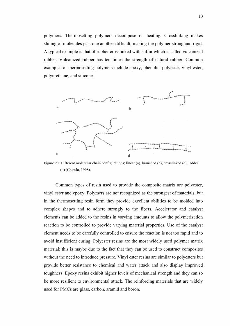
10
polymers. Thermosetting polymers decompose on heating. Crosslinking makes
sliding of molecules past one another difficult, making the polymer strong and rigid.
A typical example is that of rubber crosslinked with sulfur which is called vulcanized
rubber. Vulcanized rubber has ten times the strength of natural rubber. Common
examples of thermosetting polymers include epoxy, phenolic, polyester, vinyl ester,
polyurethane, and silicone.
Figure 2.1 Different molecular chain configurations; linear (a), branched (b), crosslinked (c), ladder
(d) (Chawla, 1998).
Common types of resin used to provide the composite matrix are polyester,
vinyl ester and epoxy. Polymers are not recognized as the strongest of materials, but
in the thermosetting resin form they provide excellent abilities to be molded into
complex shapes and to adhere strongly to the fibers. Accelerator and catalyst
elements can be added to the resins in varying amounts to allow the polymerization
reaction to be controlled to provide varying material properties. Use of the catalyst
element needs to be carefully controlled to ensure the reaction is not too rapid and to
avoid insufficient curing. Polyester resins are the most widely used polymer matrix
material; this is maybe due to the fact that they can be used to construct composites
without the need to introduce pressure. Vinyl ester resins are similar to polyesters but
provide better resistance to chemical and water attack and also display improved
toughness. Epoxy resins exhibit higher levels of mechanical strength and they can so
be more resilient to environmental attack. The reinforcing materials that are widely
used for PMCs are glass, carbon, aramid and boron.
11
2.2.1.2 Metal Matrix Materials
Metals are extremely versatile engineering materials. A metallic material can
exhibit a wide range of readily controllable properties through appropriate selection
of alloy composition and thermomechanical processing method. The extensive use of
metallic alloys in engineering reflects not only their strength and toughness but also
the relative ease and low cost of fabrication of engineering components by a wide
range of manufacturing processes. The development of MMCs has reflected the need
to achieve property combinations beyond those attainable in monolithic metals alone.
Thus, tailored composites resulting from the addition of reinforcements to a metal
may provide enhanced specific stiffness coupled with improved fatigue and wear
resistance, or perhaps increased specific strength combined with desired thermal
characteristics (for example, reduced thermal expansion coefficient and conductivity)
in the resulting MMC. However, the cost of achieving property improvements
remains a challenge in many potential MMC applications.
MMCs involve distinctly different property combinations and processing
procedures as compared to either PMCs or CMCs. This is largely due to the inherent
differences among metals, polymers and ceramics as matrix materials and less so to
the nature of the reinforcements employed. Pure metals are opaque, lustrous
chemical elements and are generally good conductors of heat and electricity. When
polished, they tend to reflect light well. Also, most metals are relatively high in
density. These characteristics reflect the nature of atom bonding in metals, in which
the atoms tend to lose electrons; the resulting free electron "gas" then holds the
positive metal ions in place. In contrast, ceramic and polymeric materials are
chemical compounds of elements. Bonding in ceramics and intramolecular bonding
in polymers is characterized by either sharing of electrons between atoms or the
transfer of electrons from one atom to another. The absence of free electrons in
ceramics and polymers (no free electrons are formed in polymers due to
intermolecular van der Waals bonding) results in poor conductivity of heat and
electricity, and lower deformability and toughness in comparison to metallic
materials.

12
Metals are strong and tough. They can be plastically deformed and strengthened
by a wide variety of methods. Metal matrix composite construction is used
primarily to increase the strength of low density metals such as aluminum alloys,
copper, titanium alloys and magnesium alloys. Another reason for constructing
MMCs is to increase the wear resistance and higher temperature performance. The
matrix material can be reinforced with continuous fibers and wires or by short fibers,
whiskers or particles. The complex nature of these materials and their manufacture
limits their use to high performance applications, in industries such as, automotive,
aerospace, and power. Some of the commonly used reinforcing materials are
boron/tungsten, titanium, alumina, graphite and silicon carbide.
Particle or discontinuously reinforced MMCs have become very important
because they are less expensive than continuous fiber reinforced composites and they
have relatively isotropic properties compared to fiber reinforced composites. Use of
nanometer-sized fullerenes (a form of carbon having a large molecule consist of an
empty cage of sixty or more carbon atoms, C60 is the most common) as a reinforce-
ment has also been tried.
2.2.1.3 Ceramic Matrix Materials
Generally, ceramics consist of one or more metals combined with a nonmetal
such as oxygen, carbon or nitrogen. They have strong covalent and ionic bonds.
Ceramic materials in general have a very attractive package of properties such as
high strength and high stiffness at very high temperatures, chemical inertness, and
low density. This attractive package is defaced by one deadly defect; lack of
toughness. They are extremely susceptible to thermal shock and are easily damaged
during fabrication and/or service. It is therefore understandable that an overriding
consideration in ceramic matrix composites is to toughen the ceramics by incorpo-
rating fibers in them and thus exploit the attractive high-temperature strength and
environmental resistance of ceramic materials without risking a catastrophic failure.
There are certain basic differences between CMCs and other composites. The general
philosophy in nonceramic matrix composites is to have the fiber bear a greater
13
proportion of the applied load. This load partitioning depends on the ratio of fiber
and matrix elastic moduli, Ef/Em. In nonceramic matrix composites, this ratio can be
very high, while in CMCs, it is rather low and can be as low as unity. Another
distinctive point regarding CMCs is that because of limited matrix ductility and
generally high fabrication temperature, thermal mismatch between components has a
very important bearing on CMC performance. The problem of chemical
compatibility between components in CMCs is similar to those in MMCs (Chawla,
1998).
CMCs are highly advanced materials and their use is restricted to applications
where high strength or high toughness is required at high temperatures. The high cost
of producing CMCs has restricted their use to applications in the power generation
and aerospace applications. Silicon carbide and boron nitride and other ceramic
fibers are used to reinforce ceramics matrices, such as aluminum oxide and silicon
carbide.
2.2.2 Fibers
Fiber is a general term for a filament with a finite length that is at least 100 times
its diameter (typically 0.10 to 0.13 mm). They are the most commonly used
reinforcing materials in high performance composites as the load bearing component.
They must have high thermal stability and should not contract or expand much with
temperature. Defects can be placed on the surface to allow the fiber to interact with
the matrix, however; bulk defects should be low. In most cases, fibers are prepared
by drawing from a molten bath, and spinning or deposition on a substrate. The term
fiber is often used synonymously with filament. Some short fibers are called
whiskers which are short single-crystal fibers or filaments made from a variety of
materials ranging from 1 to 25 microns and aspect ratios between 100 and 15,000.
There are many types of fibers used in industrial applications. The most used ones
are described below. A comparison of some important characteristics of fiber
reinforcement fibers is in Table 2.1.

14
Table 2.1 Properties of reinforcement fibers (Chawla, 1998).
1 High modulus 2 Heat stabilized 3 Trademark of Du Pont 4 Chemical vapor deposition 5 Trademark of Nippon Carbon Co.
PAN-Based Carbon SiC Property
HM1 HS2 Kevlar349 E-Glass CVD4 Nicalon5 Al2O3 Boron
Diameter (µm) 7 – 10 7.6 - 8.6 12 8 - 14 100 - 200 10 - 20 20 100 - 200
Density (g/cm3) 1.95
1.75 1.45 2.55 3.3 2.6 3.95 2.6
Young’s modulus (GPa)
Parallel to fiber axis 390 250 125 70 430 180 379 385
Perpendicular to fiber axis 12 20 – 70 – – – –
Tensile Strength (GPa) 2.2 2.7 2.8 - 3.5 1.5 - 2.5 3.5 2 1.4 3.8
Strain to fracture (%) 0.5 1 2.2 - 2.8 1.8 - 3.2 – – – –
Coefficient of thermal expansion (10-6/K)
Parallel to fiber axis –0.5 – 0.1 –0.5 - 0.1 –2 - –5 4.7 5.7 – 7.5 8.3
Perpendicular to fiber axis 7 – 12 7 - 12 59 4.7 – – – –
14

15
2.2.2.1 Boron Fibers
Boron is an inherently brittle material. It is commercially made by chemical vapor
deposition (CVD) of boron on a substrate, that is, boron fiber is itself a composite as
produced (Figure 2.2). Rather high temperatures are required for this deposition
process; therefore the choice of substrate material that is used to form the core of the
finished boron fiber is limited. A fine tungsten wire or a carbon substrate can be used
for this purpose (Chawla, 1998).
Figure 2.2 Cross section of a 100 µm diameter boron fiber (Chawla, 1998).
The structure and morphology of boron fibers depend on the conditions of
deposition; temperature, composition of gasses, gas dynamics, and so on. Complex
internal stresses and defects such as voids and structural discontinuities results from
the composite nature of boron fibers and decomposition process. Therefore boron
fibers don’t show the strength of boron. They are used in a number of military
aircraft, for stiffening golf shafts, tennis rackets, and bicycle frames. One big
obstacle to the widespread use of boron fiber is its high cost compared to other
fibers. A major portion of this high price is the cost of the substrate.

16
2.2.2.2 Carbon Fibers
Carbon is a very light element and can exist in a variety of crystalline forms. Our
interest here is in the so-called graphite structure wherein the carbon atoms are
arranged in the form of hexagonal layers. Carbon in the graphitic form is highly
anisotropic and has a very dense packing (Figure 2.3.a) in the layer planes. The
lattice structure is shown more clearly in (Figure 2.3.b). The high-strength bond
between carbon atoms in the layer plane results in an extremely high modulus while
weak van der Waals type bond between the neighboring layers results in a lower
modulus in that direction. Consequently, in a carbon fiber one would like to have a
very high degree of preferred orientation of hexagonal planes along fiber direction.
a b
Figure 2.3 The densely packed graphite layer structure (a), and the hexagonal lattice structure of
graphite (b) (Chawla, 1998).
Carbon fibers are generally made by carbonization of organic precursor fibers
such as polyacrylonitrile (PAN) fibers, rayon and the ones obtained from pitches,
polyvinyl alcohol, polyamides, and phenolics. Precursor fibers undergo preoxidation,
carbonization and surface treatment. Surface oxidized carbon fibers are also
produced to increase adhesion. Also, prepregs are manufactured with various resins
(mostly epoxy and bismaleimide) to aid in the incorporation of carbon fibers. The
term prepreg is a short form of preimpregnated fibers. Prepreg thus represent an
intermediate stage in the fabrication of a polymeric composite component. Figure

17
2.4.a shows micrograph of the cross-section of carbon fiber which can be compared
with Figure 2.4.b which shows this fiber coated with nickel. The conditions of
carbonization have impact on properties of carbon fibers and their price. The least
expensive carbon fibers manufactured from PAN are produced by rapid heating
under tension from the initial orientation temperature of 300ºC to 1000ºC. This
process produces low modulus fibers. High strength fibers are heated to 1500ºC and
the high modulus fibers to 2200ºC under argon. These various conditions result in
graphite crystals with different structures which affects the mechanical performance
of fibers. Rayon is used less often because of the environmental impact of the
precursor material. In the coal-tar or petroleum pitch processes, the initial material is
polymerized by heat which helps to remove low molecular weight volatile
components. The resultant nematic liquid crystal, or mesophase, is oriented during
the spinning operation to form fibers (Wypych, 2000).
a b
Figure 2.4 Micrograph of carbon fibers (a) and nickel coated carbon fibers (b) (Wypych, 2000).
The properties of carbon fibers such as high tensile strength and modulus, good
fatigue resistance and wear lubricity, low density (lower than metal), low linear
thermal expansion coefficient, good dimensional stability, heat resistance, electrical
conductivity, ability to shield electromagnetic waves, x-ray penetrability, good
chemical stability and excellent resistance to acids, alkalis, and many solvents are
developed their applications. These properties show that carbon fibers have a high
potential use in high performance materials. Total world production of carbon fibers
is estimated 9,590 tons; North America consumes 40% of total production, Europe
and Japan 21% each and the remaining countries 18% (Wypych, 2000). The largest

18
use is in aircraft industry followed by sport and leisure equipment and industrial
equipment.
2.2.2.3 Ceramic Fibers
Although production of ceramic fibers began in the 1940s, their commercial
exploitation did not occur until the early 1970s. Worldwide production of ceramic
fibers in the early-to-mid 1980s was estimated at 70 to 80 million kg, with U.S.
production comprising approximately half that amount. With the introduction of new
ceramic fibers for new uses, production has increased significantly over the past
decades (IARC, 1988).
Ceramic fibers comprise a wide range of amorphous or crystalline, synthetic
mineral fibers characterized by their refractory properties (i.e., stability at high
temperatures). They are typically made of alumina, silica, and other metal oxides or,
less commonly, of nonoxide materials such as silicon carbide. Most ceramic fibers
are composed of alumina and silica in an approximate 50/50 mixture. Monoxide
ceramics, such as alumina and zirconia, are composed of at least 80% of one oxide,
by definition; generally they contain 90% or more of the base oxide and specialty
products may contain virtually 100%. Nonoxide specialty ceramic fibers, such as
silicon carbide, silicon nitride, and boron nitride, have also been produced. Since
there are several types of ceramic fibers, there is also a range of chemical and
physical properties. Most fibers are white to cream in color and tend to be
polycrystallines or polycrystalline metal oxides (Figure 2.5).
Continuous ceramic fibers present an attractive package of properties. They
combine rather high strength and elastic modulus with high-temperature capability
and a general freedom from environmental attack. These characteristics make them
attractive as reinforcements in high-temperature structural materials. There are three
ceramic fiber fabrication methods: chemical vapor deposition, polymer pyrolysis,
and sol-gel techniques.

19
Figure 2.5 Optical micrograph of ceramic fiber (Chawla, 1998).
Ceramic fibers are used as insulation materials and are significant replacements
for asbestos. Due to their ability to withstand high temperatures, they are used
primarily for lining furnaces and kilns. Their light weight, thermal shock resistance,
and strength make them useful in a number of industries. High-temperature resistant
ceramic blankets and boards are used in shipbuilding as insulation to prevent the
spread of fires and for general heat containment. Ceramic textile products, such as
yarns and fabrics, are used extensively in such end-products as heat resistant
clothing, flame curtains for furnace openings, thermocoupling and electrical
insulation, gasket and wrapping insulation, coverings for induction-heating furnace
coils, cable and wire insulation, infrared radiation diffusers, insulation for fuel lines
and high pressure portable flange covers. Fibers that are coated with Teflon® are
used as sewing threads for manufacturing high-temperature insulation shapes for
aircraft and space vehicles. The spaces between the rigid tiles on space shuttles are
packed with this fiber in tape form.
2.2.2.4 Glass Fibers
Common glass fibers are silica based (~50-60% SiO2) and contain a host of other
oxides (calcium, boron, sodium, aluminum, iron etc.). Table 2.2 gives the
composition of some commonly used glass fibers. The designation E stands for
electrical because E glass is good electrical insulator in addition to having good

20
strength and a reasonable Young’s modulus; C stands for corrosion because C glass
has a better resistance to chemical corrosion; S stands for the high silica content that
makes S glass withstand higher temperatures than other types of glasses.
Table 2.2 Approximate chemical compositions of some glass fibers (Chawla, 1998).
Composition E Glass C Glass S Glass
SiO2 55.2 65 65 Al2O3 8 4 25 CaO 18.7 14 – MgO 4.6 3 10 Na2O 0.3 8.5 0.3 K2O 0.2 – – B2O3 7.3 5 –
Glass fibers are produced by two methods, milling and chopping. The milled
fibers are milled using a hammer mill which results in a relatively broad (but
consistent) length distribution. The diameter depends on the filament diameter
manufactured for milling process. The chopped fibers are produced by chopping a
bundle of glass filaments to a precise length. The length of chopped fibers is
substantially larger than that of the milled fibers. In both cases, fibers may or may
not contain sizing or surface modification. If sizing is applied, it is optimized for a
certain type or types of polymers. Cationic sized milled fiber is suggested for
polyester epoxy, phenolic and thermoplastics. Silane modified grades are for
urethanes and thermoplastics, and glass fiber without any sizing agent is suggested
for use in PTFE (Poly Tetra Fluoro Ethylene) and thermoplastics (Wypych, 2000).
Glass fibers are extensively used by industry for reinforcement of polyester,
epoxy, and phenolic resins and for the improvements they produce in thermal
properties such as reduction in thermal expansion and increase in heat deflection
temperature. Moisture decreases glass fiber strength and they are also susceptible to
static fatigue. Available glass fiber forms are given in Figure 2.6.

21
a b
c d
Figure 2.6 Available glass fiber forms; fabric (a), chopped strand (b), roving (c), continuous yarn (d)
(Chawla, 1998).
2.2.2.5 Organic Fibers
In general polymeric chains assume a random coil configuration; therefore the
molecular chains are neither aligned in one direction nor stretched out. Thus, they
have predominantly weak van der Waals interactions rather than strong covalent
interactions, resulting in a low strength and stiffness. However, if oriented molecular
chains are obtained and packed in parallel, strong and stiff polymers can be
produced. Natural organic fibers such as cellulose or synthetic organic fibers can be
used in composite materials. Two very different approaches have been taken to make
high-modulus synthetic organic fibers. These are:

22
1. Processing the conventional flexible-chain polymers in such a way
that the internal structure takes a highly oriented and extended-chain
arrangement. Structural modification of "conventional" polymers such
as high-modulus polyethylene was developed by choosing appropriate
molecular weight distributions, followed by drawing at suitable temperatures to
convert the original folded-chain structure into an oriented,
extended chain structure.
2. The second, radically different, approach involves synthesis, followed by
extrusion of a new class of polymers, called liquid crystal polymers. These
have a rigid rod molecular chain structure. The liquid crystalline state,
as we shall see, has played a very significant role in providing highly
ordered, extended chain fibers.
These two approaches have resulted in two commercialized high-strength and
high-stiffness fibers, polyethylene and aramid.
2.2.2.5.1 Cellulose Fibers
Cellulose fibers offer many valuable properties but the most important
characteristic is that they are natural in origin. They are safe to use, non-polluting,
and energy efficient. These qualities are the major reasons for the growing interest in
these fibers. Technical cellulose fibers are produced by recycling of newsprint,
magazines, and other paper products. There are also numerous industrial applications
for these fibers which exploit their chemical functionality (reactivity) for
crosslinking, their ability to retain water and their hydrogen bonding capability for
improvement of rheological properties. The shape of fiber helps to prevent cracking,
reduce shrinkage, increase green strength, and reinforce materials.
Virgin fibers produced from wood pulp contain 99.6% cellulose and they are
white. Fibers manufactured from reclaimed materials contain 75% and they are gray
23
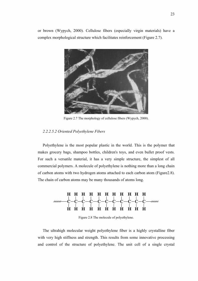
or brown (Wypych, 2000). Cellulose fibers (especially virgin materials) have a
complex morphological structure which facilitates reinforcement (Figure 2.7).
Figure 2.7 The morphology of cellulose fibers (Wypych, 2000).
2.2.2.5.2 Oriented Polyethylene Fibers
Polyethylene is the most popular plastic in the world. This is the polymer that
makes grocery bags, shampoo bottles, children's toys, and even bullet proof vests.
For such a versatile material, it has a very simple structure, the simplest of all
commercial polymers. A molecule of polyethylene is nothing more than a long chain
of carbon atoms with two hydrogen atoms attached to each carbon atom (Figure2.8).
The chain of carbon atoms may be many thousands of atoms long.
Figure 2.8 The molecule of polyethylene.
The ultrahigh molecular weight polyethylene fiber is a highly crystalline fiber
with very high stiffness and strength. This results from some innovative processing
and control of the structure of polyethylene. The unit cell of a single crystal

24
(orthorhombic) of polyethylene has the dimensions of 0.741, 0.494, and 0.255 nm
(Chawla, 1998). There are four carbon and eight hydrogen atoms per unit cell. Its
strength and modulus are slightly lower than those of aramid fibers but on a per-unit-
weight basis, specific property values are about 30% to 40% higher than those of
aramid. As is true of most organic fibers, both polyethylene and aramid fibers must
be limited to low-temperature (lower than 150°C) applications. High-modulus
polyethylene fibers are hard to bond with any polymeric matrix. Some kind of sur-
face treatment must be given to the polyethylene fiber to bond with resins such as
epoxy and (PMMA). Photomicrographs of polyethylene fibers are given in Figure
2.9.
Figure 2.9 Photomicrographs of polyethylene fibers (Wypych, 2000).
2.2.2.5.3 Aramid Fibers
Aramid fiber is a generic term for a class of synthetic organic fibers called
aromatic polyamide fibers. The U.S. Federal Trade Commission gives a good
definition of an aramid fiber as “a manufactured fiber in which the fiber-forming
substance is a long-chain synthetic polyamide in which at least 85% of the amide
linkages are attached directly to two aromatic rings”. The basic chemical structure of
aramid fibers consists of oriented para-substituted aromatic units, which make them
rigid rodlike polymers (Figure 2.10). The rigid rodlike structure results in a high
glass transition temperature and poor solubility, which makes fabrication of these
polymers, by conventional techniques, difficult.
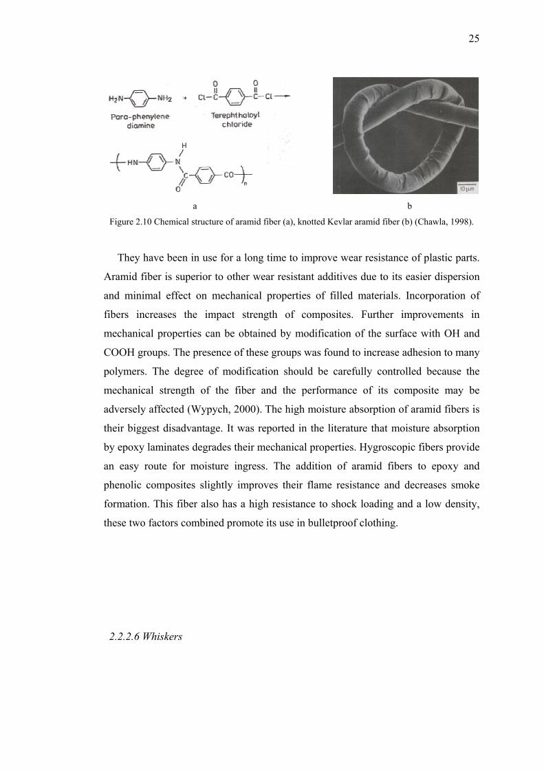
25
a b
Figure 2.10 Chemical structure of aramid fiber (a), knotted Kevlar aramid fiber (b) (Chawla, 1998).
They have been in use for a long time to improve wear resistance of plastic parts.
Aramid fiber is superior to other wear resistant additives due to its easier dispersion
and minimal effect on mechanical properties of filled materials. Incorporation of
fibers increases the impact strength of composites. Further improvements in
mechanical properties can be obtained by modification of the surface with OH and
COOH groups. The presence of these groups was found to increase adhesion to many
polymers. The degree of modification should be carefully controlled because the
mechanical strength of the fiber and the performance of its composite may be
adversely affected (Wypych, 2000). The high moisture absorption of aramid fibers is
their biggest disadvantage. It was reported in the literature that moisture absorption
by epoxy laminates degrades their mechanical properties. Hygroscopic fibers provide
an easy route for moisture ingress. The addition of aramid fibers to epoxy and
phenolic composites slightly improves their flame resistance and decreases smoke
formation. This fiber also has a high resistance to shock loading and a low density,
these two factors combined promote its use in bulletproof clothing.
2.2.2.6 Whiskers
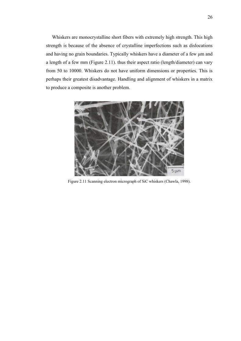
26
Whiskers are monocrystalline short fibers with extremely high strength. This high
strength is because of the absence of crystalline imperfections such as dislocations
and having no grain boundaries. Typically whiskers have a diameter of a few µm and
a length of a few mm (Figure 2.11). thus their aspect ratio (length/diameter) can vary
from 50 to 10000. Whiskers do not have uniform dimensions or properties. This is
perhaps their greatest disadvantage. Handling and alignment of whiskers in a matrix
to produce a composite is another problem.
Figure 2.11 Scanning electron micrograph of SiC whiskers (Chawla, 1998).
CHAPTER THREE
THERMAL EXPANSION BEHAVIOUR OF FIBER REINFORCED
COMPOSITES
3.1 Coefficient of Thermal Expansion (CTE)
An increase in temperature causes the vibrational amplitude of the atoms in the
crystal lattice of the solid to increase. Therefore the average spacing between the
atoms increases, causing the material to expand. If the temperature change, ∆T, is
such that the material does not go through a phase change, then the coefficient of
volumetric thermal expansion (αv) (Callister, 1994) of a material is defined as
⎟⎠⎞
⎜⎝⎛∂∂
=TV
V1α v (3.1)
where V is the total volume of the material. If we consider one dimension only, we
obtain the coefficient of linear thermal expansion (αl) as
⎟⎠⎞
⎜⎝⎛∂∂
=T
1α lll (3.2)
where l is the total length of the body. If the length increases approximately linearly
with the temperature in the temperature range observed and
0lll −=∆ (3.3)
is small when compared with the initial length l0, then coefficient of linear thermal
expansion can be written as
T
1α0 ∆⋅
∆=
ll
l (3.4)
27
28
3.2 Factors Affecting the Coefficient of Thermal Expansion
Factors affecting the thermal expansion coefficient of composite materials are:
fiber and void volumes, lay-up angle, thermal cycling, temperature dependence,
moisture effects and material viscoelasticity.
3.2.1 Fiber Volume
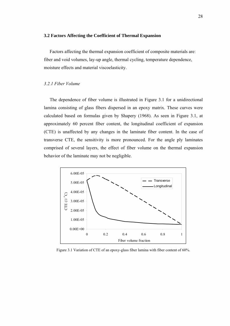
The dependence of fiber volume is illustrated in Figure 3.1 for a unidirectional
lamina consisting of glass fibers dispersed in an epoxy matrix. These curves were
calculated based on formulas given by Shapery (1968). As seen in Figure 3.1, at
approximately 60 percent fiber content, the longitudinal coefficient of expansion
(CTE) is unaffected by any changes in the laminate fiber content. In the case of
transverse CTE, the sensitivity is more pronounced. For the angle ply laminates
comprised of several layers, the effect of fiber volume on the thermal expansion
behavior of the laminate may not be negligible.
0.00E+00
1.00E-05
2.00E-05
3.00E-05
4.00E-05
5.00E-05
6.00E-05
0 0.2 0.4 0.6 0.8 1
Fiber volume fraction
CTE
(1/ o C)
TransverseLongitudinal
Figure 3.1 Variation of CTE of an epoxy-glass fiber lamina with fiber content of 60%.

29
3.2.2 Void Volume
The direct effect of voids on the CTE of composites is small within the bounds of
practical manufacturing requirements (1.5 percent max. void volume) (Johnson,
R.R., Kural M.H., & Mackey G.B. 1981). However the presence of voids can
indirectly affect the CTE of a composite by initiating microcracks in the matrix.
Voids in the matrix also tend to increase the potential moisture content of the matrix.
3.2.3 Lay-up Angle
One of the main advantages of laminated fiber reinforced composites is that
mechanical and thermal response of composites can be tailored directionally to
satisfy design requirements. This is accomplished by varying the orientation of each
layer in a systematic manner to reach the desired effect. Figure 3.2 shows the
variation of CTE of unidirectional composites with fiber orientation.
Figure 3.2 Variation of CTE of composite with fiber orientation.
The sensitivity of the composite CTE to variations of fiber orientations can be
severe. Although manufacturing tolerances for the lay-up angles are typically ±3o,
this practice can lead to serious CTE deviations for dimensionally critical structures
(Johnson, R.R. et al. 1981).

30
3.2.4 Thermal Cycling
The primary influence of thermal cycling on CTE of composites is to induce
matrix microcracking. When microcracking occurs composite becomes partially
decoupled. Matrix degradation proceeds gradually at first, and then somewhat more
rapidly, and can be detected by changes in the composite thermal response.
Therefore CTE of the composite changes. This drift depends on many factors
including materials, rate and number of thermal cycles, temperature extremes, and
mechanical load level and lay-up angle.
3.2.5 Temperature Dependence
It is a common way to report the CTE of materials as a single quantity and these
values are often used by designers and analysts in the same manner. This practice
may precipitate significant errors in composite design because of the temperature
dependence of the thermal expansion behavior of composite materials. This
temperature dependence is mainly caused by the mechanical and physical changes in
the resin system. The CTE is a calculated value which is the slope of the thermal
strain-temperature curve between two temperature and the CTE values should be
obtained from thermal expansion test data for the specific design temperature.
3.2.6 Moisture Effects
The dimensional stability of composites is highly affected by exposure to
complex hygrothermal histories. Moisture causes swelling and plasticization of the
resin system. The swelling phenomenon alters internal stresses, thus causing a
dimensional change in the laminate. Coupled with plasticization of the resin system,
permanent dimensional changes up to 30 percent have been observed in laboratory
experiments after exposure to complex hygrothermal histories. Dimensional changes
caused by a temperature change are much less than the dimensional change due to
moisture exposure. It is therefore important to account for moisture effects in
assessing dimensional changes due to thermal effects.

31
3.2.7 Viscoelasticty
Changes in the internal stresses due to moisture and thermal environment can
result in significant dimensional changes in composites. Internal stress levels also
change due to the viscoelastic phenomenon called the relaxation of the matrix.
Actually, relaxation of the internal stresses is a continuous process even without any
mechanical, thermal or moisture excursions. This process is usually minimized by
placing fibers in the direction where dimensional stability is required.
3.3 Thermal Expansion Measurement Techniques
Thermal expansion measurements can be made by mechanical dilatometry,
optical interferometry, or strain gauging methods. Each method has its strengths and
limitations in terms of quality of data, repeatability and calibration issues. Factors
affecting the results are internal stress distributions in the composites themselves,
applied forces, and the representative nature of the volume of material being sampled
by the technique.
One of the key points arising from an experimental study by Morrell (1997) is the
importance of the composite test-piece having a representative volume. Interruption
of the reinforcement by cutting free surfaces influences the internal stresses, and this
can influence the recorded thermal expansion data. The test-piece therefore needs to
be large enough that the reinforcement can be considered substantially homogeneous
and that effects of the cut edges and the local inhomogeneities can be ignored. For
in-plane measurements on continuous fiber polymer matrix composites it is preferred
to use a square plate test-piece. The effect is not thought to be significant in
homogeneous particulate reinforced materials. Further, in long-fiber multi-ply
materials it seems to be important to ensure that the through-thickness structure is
symmetrical, so that no bending occurs. Normally, composites are designed with
symmetrical lay-ups to prevent this, but manufacturing processes do not always
guarantee perfect balance. Machining test-pieces to a less than normal thickness will
unbalance the structure, and could lead to bending during thermal cycling.

32
3.3.1 Mechanical Dilatometry
This is a well established technique and commercial equipment is readily
available. A test piece in bar form is held against a stop in a support tube, and its free
end is contacted by a push road. As the test-piece is heated or cooled, its changes in
length are transmitted by the push-rod to a measurement device, usually a
displacement transducer.
Figure 3.3 Operation principle of a mechanical dilatometer (http://www.anter.com/TN69.htm).
In principle, one can devise a simple arrangement in which the movement is
transmitted out of the controlled environments and into the ambient by holding the
sample between two rods which extend outside of the heated region as shown on
Figure 3.3. The sample pushes the two rods (A and B) as it is being heated, and will
expand an amount shown by the shaded area called sample displacement, ∆lS. By
examining the experimental model, it becomes immediately clear that this
configuration will not produce the desired ∆lS on transducers. Since portions of both
rods A and B are in the controlled environment, it is inevitable that they themselves
will also expand (∆lA and ∆lB respectively). Thus, the measured value of transducer
displacement (∆XA+∆XB) will contain (∆lA+∆lB) in addition to ∆lS. The sample’s
length change, ∆lS, can therefore be written as:
( ) ( )BBAAs lXlXl ∆−∆+∆−∆=∆ (3.5)
33
Unless values of ∆lA and ∆lB are assigned, the true magnitude of ∆lS cannot be
determined from the measured values of ∆XA and ∆XB alone. Obviously, if ∆lA and
∆lB are not present at all, the measurement becomes absolute, but as long as this is
not the case, the measurement is, in principle, a relative one.
Calibration routines are also well established, and have been incorporated into
standards. The key factors in calibration are the absolute sensitivity of the
displacement measuring device, the temperature homogeneity of the system, which
can lead to a "baseline" shift (positive or negative apparent displacements with no
test-piece present), and the correction for the expansion of the apparatus itself which
the test-piece’s length is compared against. It is necessary to set up a calibration
procedure to identify these factors, to ensure that they are consistent and to use them
to correct the direct output for an unknown to the true thermal expansion behavior.
There are several options for doing this. One possibility is to run the apparatus with
two very different reference materials for which the expansion data are known. The
difference in output is then directly related to the difference in responses of the
apparatus for the two materials. The actual output of either reference material, but
usually the one with characteristics closest to those of the apparatus material itself,
can be used to obtain the apparatus expansion characteristic. Other ways to calibrate
the sensitivity of the measuring device are directly using a micrometer for displacing
it to known amounts, to run the apparatus with no test-piece to obtain the baseline
shift and to use a single reference material to determine the correction for the
apparatus expansion. In either case, the reproducibility and reliability of the
calibrations have limitations imposed primarily by the repeatability of mechanical
contacts between the test-piece or reference pieces and the apparatus, which in turn
relates to how the test-piece is held in the apparatus, and the conditions of its end
contacts. These limitations are generally poorly understood, and lead to the quotation
of results to unwarranted numbers of significant figures.
Typically, a mechanical dilatometer operated with care and attention to
repeatability of calibrations and measurement procedures can achieve a
reproducibility of about ± 0.2 x 10⁻⁶ K-1 measured over a range of 100 K, with an
34
absolute accuracy of about ± 0.2 x 10⁻⁶ K-1. Thus over large temperature ranges, the
absolute accuracy can be better than this, and over smaller temperature ranges, rather
worse. The accuracy is best treated in this manner, because the limiting mechanical
instabilities are present whatever the expansion coefficient of the material, and the
sensitivity factor (a single temperature independent figure) can usually be determined
rather more accurately than the other temperature dependent factors (Morrell, R.
1997).
The push-rod in a mechanical dilatometer normally applies a compressive axial
force on the test-piece to maintain constant contact. Typically this force is 0.5 – 2 N,
but may be less if a balanced thermomechanical analyzer type of apparatus is used.
This force may be sufficient to induce permanent distortion in composites when the
matrix phase softens. In polymer-based systems, this can happen above 150°C, and
in aluminum alloy based metal-matrix composites, above about 450°C. The
distortion may be limited to "bedding down" of the contact surfaces, but in some
cases, may induce bulk creep effects. The progressive "ratcheting" seen in repeat
thermal cycling of some composites may in part be attributable to creep effects. The
effects tend to be negligible parallel to the reinforcement directions in long-fiber
composites, but may be considerable across ply structures in 2D laminates (Morrell,
R. 1997).
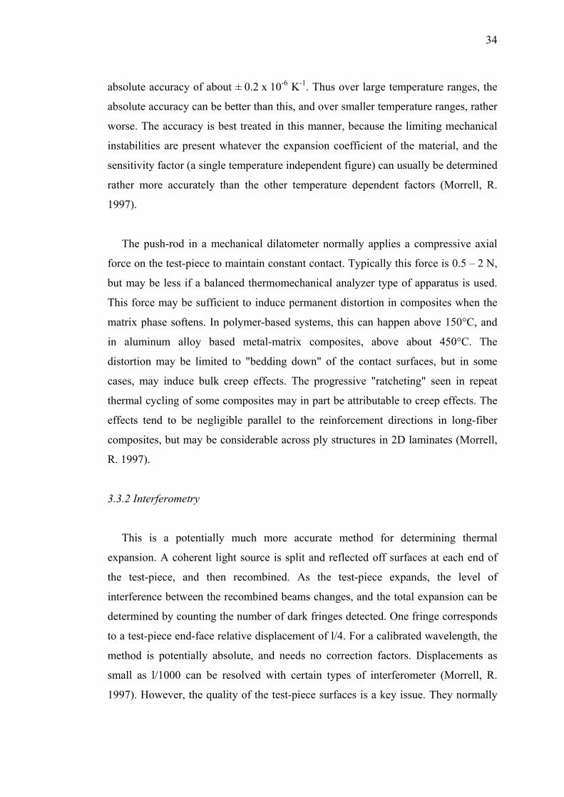
3.3.2 Interferometry
This is a potentially much more accurate method for determining thermal
expansion. A coherent light source is split and reflected off surfaces at each end of
the test-piece, and then recombined. As the test-piece expands, the level of
interference between the recombined beams changes, and the total expansion can be
determined by counting the number of dark fringes detected. One fringe corresponds
to a test-piece end-face relative displacement of l/4. For a calibrated wavelength, the
method is potentially absolute, and needs no correction factors. Displacements as
small as l/1000 can be resolved with certain types of interferometer (Morrell, R.
1997). However, the quality of the test-piece surfaces is a key issue. They normally
35
need to be optically flat and reflective to act as their own mirrors. If this is
impossible, as is usually the case with composite materials, mirrors need to be placed
on the end surfaces, which poses questions of mechanical stability and correction for
the expansion of the mirrors. Figure 3.4 illustrates the basic features of a Michelson
laser interferometer.
Figure 3.4 Basic illustration of the Michelson laser (http://www.pmiclab.com/index.html).
Other factors requiring consideration are alignment of the mirrors, temperature
homogeneity of the test-piece and the temperature stability needed to obtain stable
fringes. In addition, the measurement normally has to be conducted in vacuum to
avoid the distorting effects of convection in air along the beam path. The technique is
best suited to accurate measurements near room temperature, particularly on low
thermal expansion materials.
Separate mirrors have to be used because composites cannot be adequately
polished to give reflective surfaces. Resting the test-piece stably on a mirror and
placing a second mirror on the top surface is the simplest configuration to use. The
test-piece surfaces need to be accurately flat and parallel, and moulded surfaces may
have to be machined to achieve the alignment conditions required for the mirrors.
Care is needed not to unbalance systems in such a machining process. Typically, test-
pieces might be quite small, but for larger items made from low thermal expansion
materials, carefully aligned mirrors can be glued to a face of the composite in order
to achieve representative lengths to measure expansion.

36
3.3.3 Strain Gauges
This relatively little-used technique has been evaluated on composite materials
and found to be quite promising provided care is taken over calibration routines
(Morrell, R. 1997). The technique used employs a thermal expansion reference
material with an identical strain gauge attached to it and wired so that the differential
expansion is recorded. There are considerable advantages in this technique for
examining the spatial homogeneity of expansion or dimensional stability of large
pieces inappropriate for dilatometry or interferometry. The main drawback is the
temperature limitation of the gauge and the means of securing it to the material.
Conventional foil gauges can be used typically to 200°C, and although higher-
temperature versions and appropriate adhesives can be obtained, they are relatively
expensive and specialized, so that 200°C should be taken as the upper temperature
limit.
It is essential that identical installation techniques are employed on the test-piece
and on the reference, and that the reference is well characterized over the required
temperature range. In the tests they must also be at identical temperatures, and thus
this technique should ideally to be performed at a series of temperature holds with
stabilization periods, unless the test-pieces have sufficiently small thermal masses
that the test can be done reliably during temperature ramping.
The technique had been validated using copper and aluminum with ULE silica
(Corning Glass Works, near zero expansion coefficient glass) as the zero reference
(Morrell, R. 1997). Questions of the lateral sensitivity of strain gauges do not apply
to isotropic materials as the test-pieces are not mechanically strained, and any
secondary effects are eliminated in the difference calculations. Comparisons between
mechanical dilatometry and the strain gauge technique had been carried out on metal
matrix composites by Morrell (1997), and a good match was found to 200°C, above
which the properties of the gauge and/or its adhesive affected the results. With
anisotropic materials, lateral sensitivity is more important, and increases the potential
errors in the results.

37
The area covered by a strain gauge is usually quite small, 1-5 mm, and this means
that it samples the local behavior rather than the longer range average. In composites
which have homogeneous reinforcement, such as flat laminates, unidirectional
reinforcements and particulate composites, the technique can be used reliably, but
caution needs to be exercised with woven structures. The active part of the strain
gauge needs to cover several representative reinforcement units for the results to be
representative of bulk material behavior.
3.4 Theoretical Consideration
Micromechanics is a study of mechanical properties of composites in terms of
those of constituent materials (Tsai, & Hahn 1980). In discussing composite
properties it is important to define a volume element which is small enough to show
the microscopic structural details, yet large enough to represent the overall behavior
of the composite. Such a volume element is called the representative volume
element. A simple representative volume element can consist of a fiber embedded in
matrix block.
Once a representative volume element is chosen, proper boundary conditions are
prescribed. Ideally, these boundary conditions must represent the in situ states of
stress and strain within the composite. That is, the prescribed boundary conditions
must be the same as those if the representative volume element were actually in the
composite.
Finally, a prediction of composite properties follows from the solution of the
forgoing boundary value problem. Although the procedure involved is conceptually
simple, the actual solution is rather difficult. Consequently, many assumptions and
approximations have been introduced, and therefore, various solutions are available.
General assumptions in micromechanics of composites are:

38
• The composite is macroscopically homogeneous and orthotropic, linearly
elastic, initially stress free, and free of voids. There is complete bonding at
the interface of the constituents and there is no transitional region between
them. The displacements are continuous across the fiber matrix interphase
(there is no interfacial slip).
• The fibers are homogeneous, linearly elastic, isotropic or orthotropic,
regularly spaced, perfectly aligned, circular in cross section, and infinitely
long in the longitudinal direction.
• The matrix is homogeneous, linearly elastic, and isotropic.
• The temperature is uniform and remains uniform during the temperature
increase. Constituent material properties do not vary with temperature.
3.4.1 Some of the Existing Theories
Consider a random two-phase composite. Assuming that one of the phases,
subscript f, is dispersed in a polymer phase, subscript m, and αm > αf, where α is the
thermal expansion coefficient of the phases. When such a composite is heated, even
under conditions of no external loading, the matrix will wish to expand more than the
fillers and if the interface is capable of transmitting the stresses which are set up as a
result of differences between the thermal expansion coefficients and elastic constants
of the constituents so that the expansion of the matrix will be reduced. These thermal
stresses cause stress concentrations which may initiate yielding or debonding.
Therefore, in design analysis, it is important to understand how these stresses arise
and how to control the thermal expansion coefficients of the composite. In the
theoretical treatments to be described, except for the equations of Sideridis (1994), it
is assumed that the adhesion at the interface is adequate to withstand this task.
3.4.1.1 Law of Mixtures
If each phase is assumed homogeneous and isotropic and linearly elastic over a
small range of volumetric strains, in the absence of the phase interaction, one may

39
expect the coefficient of thermal expansion of a composite to follow simple law of
mixtures given by:
mmffc υαυαα += (3.6)
where αc, αf, αm are thermal expansion coefficients of the composite, filler and matrix
respectively and υf and υm are the volumetric fractions of the filler and the matrix.
Because of the differences in the thermal expansivities of the phases a state of
micro-stress often exists between them. These stresses influence the thermal
expansion behavior of the body. Thus, its thermal expansion coefficient does not
follow the rule of mixtures.
3.4.1.2 Equation of Thomas
Thomas (Sideridis, 1994) put forward an empirical solution which can be written
as
mamf
af
ac υαυαα += (3.7)
where a may vary from -1 to +1, and γ is the volumetric thermal expansion
coefficient which is defined as αc = 3α for an isotropic composite. However, for a
unidirectional composite, which is isotropic in the two transverse directions, the
relation between volumetric thermal expansion coefficient and longitudinal and
transverse thermal expansion coefficients can be written as
21c α2αα += (3.8)
where α1 is the thermal expansion coefficient in the longitudinal direction and α2 is
the thermal expansion coefficient in the transverse direction. The empirical nature of
the equation makes it suitable for most filed systems by the correct use of the
adjustable constant.

40
3.4.1.3 Equation of Van Fo Fy
In a series of articles by Van Fo Fy (1965), thermal expansion coefficients for
matrices reinforced by continuous fibers are developed by means of a detailed stress
analysis. As a result of this work, the thermal expansion coefficient in the
longitudinal direction (α1) is
( )( ) ( )( )( ) 1f12m
mm1f12ffmfmm1 Eνν
υEEν1υEν1αααα−
−+−+−−= (3.9)
and the thermal expansion coefficient in the transverse direction (α2) is
( ) ( )( )f12m
12mf12fm121mm2 νν
ννν1ααναααα−−
+−−−+= (3.10)
where Ef, Em are elastic moduli and νf, νm are the Poisson’s ratios of fiber and matrix
respectively. E1 is the elastic modulus for the longitudinal direction of composite and
ν12 is the Poisson’s ratio of the composite. However, the values predicted by these
expressions are very sensitive to variations in E1 and deviations arose by the
experimental error may cause considerable discrepancies. E1 can be found, using the
simple rule of mixtures, as
mmff1 υEυEE += (3.11)
3.4.1.4 Equation of Cribb
Cribb (Sideridis, 1994) adopted an approach in which no limitations are made on
the shape or size of the fillers. The phases are assumed to be homogeneous, isotropic
and linearly elastic. The equation is given as
f2m1c αθαθα += (3.12)

41
where
( )( )
( )( )fmc
cmf2
fmc
fcm1 KKK
KKKθ ,
KKKKKK
θ−−
=−−
= (3.13)
In these equations Kc, Kf and Km represent the bulk moduli of the composite, filler
and matrix respectively. The simplicity of this approach is attractive, but it converts
the problem of calculating α c to knowledge of Kc or an ability to calculate it from the
properties and volume fractions of the individual components.
3.4.1.5 Equation of Schapery
Schapery (1968) has derived expressions for the longitudinal and transverse
effective thermal expansion coefficients both for isotropic and anisotropic
composites consisting of isotropic phases, by employing extremum principles of
thermoelasticity.
He considered a specimen under a space wise uniform temperature in the form of
a rectangular parallelepiped whose edges are parallel to coordinate axes and with unit
volume. This specimen is statistically homogeneous and composed of n phases
(constituents), each of which has homogeneous mechanical and thermal properties
that are different from any other phase. No restriction is placed on the temperature
dependence of constituent properties. Maximum dimensions defining the specimen’s
structural inhomogeneity are assumed small compared to specimen dimensions and
the interaction between phases is considered to be purely mechanical and linear. Also
specimen and phases are assumed unstressed and unstrained when surface tractions
are zero and the temperature is at some reference value.
As a result, for a unidirectional two phase composite, the thermal expansion
coefficient in the longitudinal direction is
mmff
mmmfff1 υEυE
υαEυαEα++
= (3.14)

42
and the thermal expansion coefficient in the transverse direction is
( ) ( ) ( )mmff1mmmfff2 υνυναυαν1υαν1α +−+++= (3.15)
3.4.1.6 Equation of Chamberlain
An alternative model for transverse thermal expansion of unidirectional
composites was derived by Chamberlain (Rogers et al., 1977), using plane stress
thick walled cylinder equations for the case of transversely isotropic fibers in an
isotropic matrix. The equation for the longitudinal thermal expansion coefficient is
similar to Schapery’s formula and can be written as
mmff1
mmmff1f11 υEυE
υαEυαEα++
= (3.16)
where Ef1 is the elastic modulus of fiber for the longitudinal direction and αf1 is the
thermal expansion coefficient of fiber in the longitudinal direction. The expression
for thermal expansion coefficient in the transverse direction takes the form
( )( ) ( ) ( )( )mf12
f1
mfmm
fmf2m2
υ1-Fν1EEυFυ1-Fν
υα-α2αα+−++++
+= (3.17)
where αf2 is the thermal expansion coefficient of fiber in the transverse direction, νf12
is the Poisson’s ratio of the fiber and F is a packing factor which accounts for fiber
packing geometry (Figure 3.5), and is equal to 0.9069 for hexagonal packing and for
0.7854 for square packing respectively.

43
Square packing Hexagonal packing
Figure 3.5 Idealized fiber packing arrangements.
3.4.1.7 Equation of Rosen and Hashin
Rosen and Hashin (1970) derived expressions for the effective thermal expansion
coefficients of multiphase composites and the summary of their approach for
unidirectional fiber reinforced composites with transversely isotropic constituents is
given as
( ) ( ) ( )[ ]( ) ( ) ( ) ([ ]2322m2f212m1f11212
12m2f211m1f1111111
PP2αα2Pαα SS
2PααPαα SSαα
+−+−−+
−+−−+=
) (3.18)
( ) ( ) ( )[ ]( ) ( ) ( )([ ]( ) ( ) ( )([ ]3323m2f212m1f12323
2322m2f212m1f12222
12m2f211m1f1121222
PPααPαα SS
PPααPαα SS
2PααPαα SSαα
+−+−−+
+−+−−+
−+−−+=
))
(3.19)
where
2
2323
1
121312
23322
111
S ,SS
1SS ,1S
EE
EEνν −
=−
==
===
(3.20)
and Pab (a,b=1,2,3) are

44
ADet AAA
P ,ADet
AAAPP
ADet AAAA
PP ,ADet AA
P
2311212
23
2122211
2233
221223121213
223
222
11
−=
−==
−==
−=
(3.21)
where Aab is defined as (Sfab - Smab) and Det A is given by
( ) ( )2212231212223
22211 AAAA2AAAAADet −+−= (3.22)
In above equations subscripts f and m refer to fiber and matrix and terms with and
without a hat refer to volume average and effective composite properties
respectively. Sab can be written for the effective property, the volume average
property and the constituent properties. Composite volume average properties are
obtained with the expression
mmff υpυpp += (3.23)
and composite effective mechanical properties are given by Hashin (1979). It is very
difficult to find the coefficients of thermal expansion of a composite using equations
of Rosen and Hashin because, to determine composite effective mechanical
properties the bulk modulus of the constituents and the composite should be
determined.
3.4.1.8 Equation of Schneider
Another consideration was made by Schneider (1971), who assumed a hexagonal
arrangement of cylindrical fiber-matrix elements consisting of a fiber surrounded by
a cylindrical matrix jacket. The equation for the longitudinal thermal expansion
coefficient is identical to Schapery’s formula. For the transverse direction he derived
the following equation
45
( ) ( )( )
⎥⎥⎥⎥
⎦
⎤
⎢⎢⎢⎢
⎣
⎡
+−
+−−
+−+
−−=
m
f
m
fm
2mm
f
f
2mm
fmm2
EE
C1
EEν
C2νν11.1υ
1.1υ1C1νν12 αααα (3.24)
in which
f
f
1.1υ11.1υC−
= (3.25)
3.4.1.9 Equation of Chamis
Chamis (1984) has used a simple force balance, or strength of materials, approach
to derive expression for both mechanical and thermal properties of unidirectional
composites with transversely isotropic fibers. The derived expression for the
longitudinal thermal expansion coefficient is again identical to Schapery’s formula.
The expression for the transverse thermal expansion coefficient is
( ) m1
f1mffff22 α
EEνυ1 υ1υαα ⎟⎟
⎠
⎞⎜⎜⎝
⎛+−+= (3.26)
3.4.1.10 Equation of Sideridis
Sideridis (1994) has calculated the expansion coefficients of the composite using
a model which introduces the concept of the boundary interphase. This concept
determines the influence of the interphase which depends on the quality of adhesion
between fiber and matrix. It has been assumed that the composite has well defined
material properties for the fiber and matrix, whereas the interphase material has
inhomogeneous properties (thermal expansion coefficient, the elastic modulus and
Poisson’s ratio) varying from the fiber surface to the matrix. He also made the
following assumptions:

46
• A perfect bonding exists at all surfaces.
• The fiber and the matrix materials carry only tensile stresses.
• The interphase material can only carry shear stresses.
The equation for the longitudinal thermal expansion coefficient is
( ) ( )
( )∫
∫+′+
+′+=
i
f
i
f
r
r i2m
mmff
r
r iimmmfff
1
drr rEr2υEυE
drr rErαυEαυEαα (3.27)
and for the transverse thermal expansion coefficient is
( ) ( ) ( )( ) ( )
( )∫
∫
+′+−
++′+++=
i
f
i
f
r
r i2m
mmff1
r
r ii2m
mmmfff2
drr rνr2υνυνα
dr rαrν1r2υαν1υαν1α
(3.28)
where rf, ri, rm are the outer radii of the fiber, the interphase and the matrix circular
sections respectively, then the fractions of the respective phases are
2m
2f
2m
m2m
2f
2i
i2m
2f
f rrrυ ,
rrr υ,
rrυ −
=′−== (3.29)
with
ifm υυ1υ −−=′ (3.30)
The influence of the mode of variation of the interphase material properties
(linear, hyperbolic and parabolic) on the thermal expansion coefficient was studied
by Sideridis. However, it is inconvenient to determine the thermal expansion
coefficient of a composite using equation of Sideridis, because determination of the

47
radius of the interphase requires making complicated experiments on the produced
samples.

CHAPTER FOUR
FINITE ELEMENT METHOD
4.1 Historical Perspective
The finite element method has become a powerful tool for the numerical solution
of a wide range of engineering problems such as steady, transient, linear or nonlinear
problems in stress analysis, heat transfer, fluid flow, and electromagnetism. With the
advantages in computer technology and computer-aided design systems, complex
problems can be modeled with relative ease. Several alternative configurations can
be tested on a computer before the first prototype is built. In this method of analysis,
a complex region defining a continuum is reduced into simple geometric shapes
called finite elements. The material properties and the governing relationships are
considered over these elements and expresses in terms of unknown values at element
corners. An assembly process, considering the loading and the constraints, results in
a set of equations. Solution of these equations gives us the approximate behavior of
the continuum.
The origin of the modern finite element method may be traced back to early
1900s, when some investigators approximated and modeled elastic continua using
discrete equivalent elastic bars. But basic ideas of the finite element method
originated from advances in aircraft structural analysis. In 1941, Hrenikoff presented
a solution of elasticity problem using the “frame network method”. Courant’s paper,
which used a piecewise polynomial interpolation over triangular subregions to model
torsion problems, appeared in 1943. Turner et al. derived stiffness matrices for truss,
beam and other elements and presented their findings in 1956. The term finite
element was first coined and used by Clough in 1960 (Chandrupatla, & Belegundu,
2002)(Moaveni, 1999).
In the early 1960s, engineers used the method for approximate solution of
problems in stress analysis, fluid flow, heat transfer and other areas. A book by
48

49
Argyris in 1955 on energy theorems and matrix methods laid a foundation for further
developments in finite element studies. The first book on finite elements by
Zienkiewicz and Chung was published in 1967. In the late 1960s and early 1970s,
finite element analysis was applied to nonlinear problems and large deformations.
Oden’s book on nonlinear continua appeared in 1972. Mathematical foundations
were laid in the1970s. New element development, convergence studies, and other
related areas are in this category. Today, the developments in main frame computers
and availability of powerful microcomputers has brought this method within reach of
students and engineers working in small industries (Chandrupatla, & Belegundu,
2002).
4.2 Finite Element Analysis Procedure
4.2.1 Geometry Creation
The first step in the finite element analysis procedure is to model the part
geometry. There are many ways to define geometry, ranging from two-dimensional
drawings to three-dimensional computer-aided design. Computer-aided drafting
permits easy generation and editing of two-dimensional geometry. In general, this
process involves placing lines, rectangles, arcs, circles, and other basic
geometric shapes on a display screen and then moving, rotating, and scaling
these shapes to define a part outline. Often, there is a need to describe a part in
three dimensions so that it can be more easily understood and converted to a
discretized finite-element definition. Wireframe modeling is the simplest approach
to graphical display of three-dimensional shapes by definition of part outlines and
intersections of surfaces. Unfortunately, these models can be obscure and difficult
to visualize. Surface modeling goes one step beyond wireframes by describing the
individual surfaces of the model, analogous to stretching a thin fabric over the
wireframe model. Solid models provide the most accurate description of part
geometry by mathematically describing the interior and exterior of the part
(Trantina, & Nimmer, 1994).

50
No matter how the geometry is created, it must eventually be described
discretely in terms of nodal points and elements in order to apply finite-element
analysis. For complex parts, this process is usually accomplished by using an
automated finite-element mesh generator to represent a part discretely in terms of
nodes and elements. In spite of the automated nature of this process, there is
often a need to apply engineering analysis judgment. For example, if a shell
finite-element model is applied, the engineer must be aware that certain
concentrations such as the corners of a box may not be adequately modeled lo-
cally with the shell analysis. This is a situation that would require a three-
dimensional analysis to define local stresses accurately if that were necessary.
Therefore, a significant amount of engineering judgment is required to produce an
effective geometric representation of a complex part.
4.2.2 Mesh Creation and Element Selection
Once the overall geometry has been defined it must be divided into elements that
are connected to one another at the nodal points. This division of the geometry into
a set of elements is referred to as a mesh. Engineering judgment is required to select
an appropriate element type, as discussed in the preceding section. Also,
engineering judgment is required to determine the mesh density and the number and
size of the elements. Coarser meshes result in faster solution times but also limit the
accuracy of the analysis. Higher mesh densities should be created in regions where
large gradients are expected. Automated meshing routines are available where the
user can specify the mesh density.

51
Figure 4.1 Examples of finite elements (Trantina, & Nimmer, 1994).
4.2.3 Boundary and Loading Conditions
Applying boundary conditions and the proper loading on a structure appear as a
very important part of the finite element solution. For static problems, the stiffness
matrix associated with the linear equations of equilibrium for the complete structure
will be singular, unless all rigid body motion is prohibited. As a result, a fundamental
requirement for solution of the linear equations governing a problem is that the
structure must be prevented from freely translating or rotating in space. Rigid body
motion is eliminated through the application of boundary conditions requiring zero

52
displacements and/or rotations at nodes. Additional displacement boundary
conditions can also be applied to the structure to model the actual structural support
system. It is not necessary to restrain all of the displacements and rotations at a node.
For the thermal analysis problems, prescribed temperatures, conductive heat flux
boundary conditions, convection boundary conditions and radiation boundary
conditions may be applied to the model.
Loads may be applied to a model either in the form of applied forces,
displacements or thermal effects. Concentrated loads can only be applied at the node
locations of the elements. Distributed loads and body loads can also be applied to
finite-element surfaces and volumes, respectively. Distributed loads are usually
internally translated to equivalent nodal loads within the finite-element code.
4.2.4 Defining Material Properties
In addition to the geometric detail of the component and the applied loads, the
material (constitutive) properties must also be defined. For simple isotropic, linear-
elastic stress analysis, only the material elastic modulus and Poisson's ratio need be
provided. In some cases, more detailed constitutive models may be desirable. For
example, for highly loaded parts, elastic-plastic behavior may be included. In some
cases, properties may be functions of time, rate, temperature, or other variables. It
must be emphasized that increased capability in modeling material behavior means in
general that more material data must be available. In many cases, such as time-
dependent material models, for example, measurements to obtain such data are
nonstandard in nature (Trantina, & Nimmer, 1994).
It must be kept in mind that, real material properties are not dependent upon
geometry and the property is only useful in the general engineering sense if it is
associated with a methodology of applying it to general geometries. Many tests are
carried out on materials as functions of rate and temperature to provide comparative
performance values. However, in many cases these measurements do not represent
true material properties because they are uniquely associated with the test geometry

53
used to make the measurement and there is no methodology available to generalize
the measurement for use in complex geometries.
4.2.5 Displaying Results
After the analyst has defined geometry, element, and node discretization,
boundary conditions, loads, and material constitutive relationships, the finite-element
code can assemble the equilibrium equations governing the structure. These
equations can vary from hundreds to thousands for typical problems. The finite-
element code solves this system of equations. As a result of this solution, a massive
amount of information is computed displacements of all nodes and stresses, strains,
temperatures, heat fluxes etc. in all elements. Fortunately, this information can be
displayed with advanced graphics techniques as constant-stress contours or with a
color-coded representation of the particular stress range of interest. These results can
then be assessed in terms of engineering performance requirements. In order to judge
whether failure will occur, material data defining failure limits in terms of stress or
strain are generally required.
CHAPTER FIVE
MICROMECHANICAL ANALYSIS BY ANSYS
5.1 Model Development
In the present work, the effective coefficient of thermal expansion (CTE) of
different kinds of fiber reinforced composites is studied by micromechanical
modeling using finite element method. To determine the both longitudinal and
transverse CTEs of composites, three dimensional steady state analyses were
undertaken.
Representative unit cell models for different fiber volume fractions and different
kind of materials were produced using finite element program ANSYS. The
representative unit cell used for the current analysis is a cylinder which is embedded
in a cube with unit dimension. Fibers are assumed to have a square packing
arrangement. The radius of the cylinder is determined with respect to fiber volume
fraction of the composite. Figure 5.1 shows the unit cell considered in the
micromechanical analysis. Using the advantage of symmetry, only an octant of the
unit cell, indicated in Figure 5.2, is modeled to describe the behavior of the unit cell
and of an entire continuum of unit cells for the finite element analysis.
To compare the results of finite element solutions for different types of
composites with the results of the analytical methods and to determine the expansion
behavior of different material systems with respect to fiber content, models having
fiber volume fractions from 10% to 80% with increments of 10% have been
composed. Furthermore, comparison between finite element solutions and
experimental results have been made upon the models having 40%, 47%, 48%, 54%,
57%, 63%, 65%, and 68% fiber volume fractions.
54
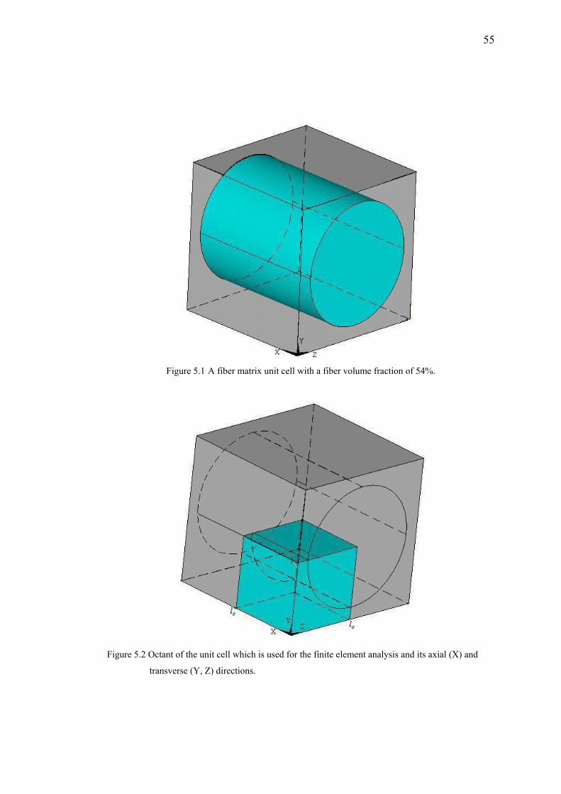
55
Figure 5.1 A fiber matrix unit cell with a fiber volume fraction of 54%.
Figure 5.2 Octant of the unit cell which is used for the finite element analysis and its axial (X) and
transverse (Y, Z) directions.
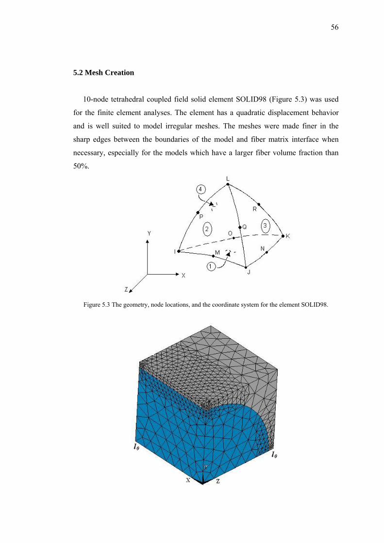
56
5.2 Mesh Creation
10-node tetrahedral coupled field solid element SOLID98 (Figure 5.3) was used
for the finite element analyses. The element has a quadratic displacement behavior
and is well suited to model irregular meshes. The meshes were made finer in the
sharp edges between the boundaries of the model and fiber matrix interface when
necessary, especially for the models which have a larger fiber volume fraction than
50%.
Figure 5.3 The geometry, node locations, and the coordinate system for the element SOLID98.
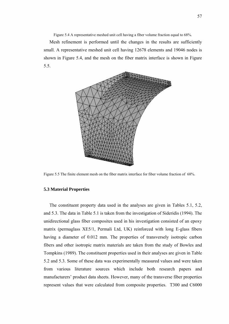
57
Figure 5.4 A representative meshed unit cell having a fiber volume fraction equal to 68%.
Mesh refinement is performed until the changes in the results are sufficiently
small. A representative meshed unit cell having 12678 elements and 19046 nodes is
shown in Figure 5.4, and the mesh on the fiber matrix interface is shown in Figure
5.5.
Figure 5.5 The finite element mesh on the fiber matrix interface for fiber volume fraction of 68%.
5.3 Material Properties
The constituent property data used in the analyses are given in Tables 5.1, 5.2,
and 5.3. The data in Table 5.1 is taken from the investigation of Sideridis (1994). The
unidirectional glass fiber composites used in his investigation consisted of an epoxy
matrix (permaglass XE5/1, Permali Ltd, UK) reinforced with long E-glass fibers
having a diameter of 0.012 mm. The properties of transversely isotropic carbon
fibers and other isotropic matrix materials are taken from the study of Bowles and
Tompkins (1989). The constituent properties used in their analyses are given in Table
5.2 and 5.3. Some of these data was experimentally measured values and were taken
from various literature sources which include both research papers and
manufacturers’ product data sheets. However, many of the transverse fiber properties
represent values that were calculated from composite properties. T300 and C6000

58
carbon fibers were assumed to have same properties. All of the epoxies were
assumed to have same properties except CE339, which has a larger CTE. This larger
value of CTE is due to the rubber particles in this rubber toughened epoxy.
Table 5.1 Material properties, at room temperature, used for the composite consisting of isotropic
glass fibers and isotropic epoxy matrix (Sideridis, 1994).
Material E (GPa) G (GPa) ν α (10-6/ºC)
Epoxy 3.5 3.89 0.35 52.5 Glass fiber 72 40 0.2 5
Table 5.2 Matrix properties at room temperature (Bowles, & Tompkins, 1989).
Matris E (GPa) G (GPa) ν α (10-6/ºC)
934 epoxy 4.35 1.59 0.37 43.92 5208 epoxy 4.35 1.59 0.37 43.92
930 epoxy 4.35 1.59 0.37 43.92
CE339 epoxy 4.35 1.59 0.37 63.36
PMR15 polymide 3.45 1.31 0.35 36
2024 Aluminum 73.11 27.58 0.33 23.22
Borosilicate glass 62.76 26.20 0.20 3.24
Table 5.3 Carbon fiber properties at room temperature (Bowles, & Tompkins, 1989).
Fiber E1 (GPa)
E2 (GPa)
G1 (GPa)
G2 (GPa) ν1 ν2
α1 (10-6/ºC)
α2 (10-6/ºC)
T300 233.13 23.11 8.97 8.28 0.2 0.4 − 0.54 10.08
C6000 233.13 23.11 8.97 8.28 0.2 0.4 − 0.54 10.08
HMS 379.35 6.21 7.59 2.21 0.2 0.4 − 0.99 6.84
P75 550.40 9.52 6.9 3.38 0.2 0.4 − 1.35 6.84
P100 796.63 7.24 6.9 2.62 0.2 0.4 − 1.40 6.84

59
5.4 Boundary Conditions
There are several basic assumptions that are common to all of the methods, which
are given in the previous chapter. In addition, the boundary conditions used in the
finite element analyses are as follows:
• Along the planes x, y, and z = 0, the model is restricted to move in the x, y,
and z directions respectively.
• The boundary planes x, y, and z = l0 are free to move but have to remain
planar in a parallel way for preserving the compatibility with adjacent cells.
5.5 Solution
The deformation in the unit cell is caused by a temperature increase of ∆T.
During the deformation; x, y, and z = l0 become, x, y, and z = l respectively and the
displacement, ∆l, is determined from the analysis. The CTE of the composite for the
direction i is then found using
∆T1∆α
0i l
l= (5.1)
For an easier solution, edge of the representative unit cell is taken as unity and
also the temperature increase is taken as unity. Then CTE of the composite for the
required direction becomes the displacement of the unit cell for that direction. The
displacement fields for the unit cell having a fiber volume fraction of 48% is given in
Figure 5.6 and Figure 5.7.

60
Figure 5.6 The displacement field in the longitudinal direction for the unit cell having a fiber volume
fraction of 48%.
Figure 5.7 The displacement field in the transverse direction for the unit cell having a fiber volume
fraction of 48%.

CHAPTER SIX
RESULTS AND DISCUSSION
Carbon fiber reinforced composite material systems had axial fiber to matrix
stiffness ratios (Ef1/Em) ranging from 6 to 140, and axial fiber to matrix coefficient of
thermal expansion (CTE) ratios (αf1/αm) ranging from −0.01 to −0.30. Besides, glass
fiber reinforced composite material had Ef/Em of 20.6, and αf/αm of 10.5. Therefore,
this investigation has covered a wide range of fiber/matrix combinations.
CTE predictions from some of the analytical models presented in Chapter 3 were
compared with each other, with available experimental data and with finite element
results for all of the material systems. Predicted and measured values for the
longitudinal and transverse directions for all of the materials studied are given in
Tables 6.1 and 6.2 respectively. The comparisons of these model predictions with
experimental data show that for some material the agreement is very good, but for
others there is some discrepancy between the experimental results and model
predictions. The reason may be that the fiber-matrix interface bond which was
assumed to be perfect was not really so in the experimental materials. The interface
may either contain interfacial cracks or it might have elastic properties different from
those of matrix and fiber.
Figures 6.1 – 6.14 show a comparison of longitudinal and transverse CTEs as a
function of fiber volume fraction, predicted from the different methods for seven
different material systems: E-Glass/Epoxy, T300/934 (T300/5208), P75/934
(P75/930), P75/CE339, C6000/PMR15, HMS/Borosilcate, and P100/2024Al.
Experimental data are also shown on these figures.
The Shapery, Chamberlain (both hexagonal and square), Schneider, and Chamis
methods all used Equation (3.14) for predicting longitudinal CTEs. As shown in the
Table 6.1 and Figures 6.1, 6.3, 6.5, 6.7, 6.9, 6.11, and 6.13, the differences between
the Rosen-Hashin and finite element results were negligible and there were only
61

62
small differences between these and the other results. All of the models and finite
element analyses were in good agreement with the experimental data for longitudinal
CTEs. The largest deviation between any of the predicted and experimental values
for longitudinal CTE was 0.22 10-6/°C only, in most cases the deviation was on the
order of about 0.1 10-6/°C, and the average deviation is 0.127 10-6/°C. Although the
magnitudes of longitudinal CTE differed for different material systems , the general
response was the same (decreasing CTE with increasing volume fraction). This
implies that the relative magnitudes of the fiber/matrix stiffness and CTE ratios did
not significantly affect the general trend in longitudinal CTE as a function of volume
fraction.
For the transverse CTE the Shapery results were obtained by using the modified
version of the Equation (3.15) for transversely isotropic fibers, replacing fiber
properties with transverse fiber properties. There were large differences between the
predicted values for all of the methods, except for the Rosen-Hashin method and
finite element analyses. Results from these two methods were in excellent agreement
with each other. The differences between Chamis and finite element results were
attributed to Poisson restraining effects which were not included in Equation (3.26).
The omission of this type of three dimensional effects was also thought to be
responsible for the large difference between the Chamberlain, Schneider, and finite
element results. These differences have been previously documented in the literature
(Bowles, & Tompkins, 1989).
Results also show that the Rosen-Hashin and finite element results for transverse
CTE were generally in much better agreement with the experimental data, than the
other methods for all materials investigated. The Shapery results were in good
agreement with experimental results and were in better agreement with the
experimental data for the P75/930 and P75/CE339 material systems. However, it
should be noted that the matrix mechanical properties for these two systems were
assumed to be the same as the other epoxy matrices, which is probably not an
accurate assumption, and therefore the better agreement with the experimental data is
believed to be coincidental. It should also be remembered that the modification of the

63
Shapery’s method for transversely isotropic fibers was not based on any
mathematical derivation, and was included for comparison purposes only. Agreement
between experimental values and Rosen-Hashin and finite element predicted values
were usually within about 15%. Predictions from the other methods differed with the
experimental data by as much as 50%. The largest deviation between any of the
predicted and experimental values for transverse CTE was 27.09 10-6/°C, in most
cases the deviation was on the order of about 10 10-6/°C, and the average deviation is
6.45 10-6/°C.
Unlike the results for longitudinal CTE, the response of transverse CTE as a
function of volume fraction was affected by the fiber/matrix property ratios. E-Glass/
Epoxy, T300/934 and P75/934, P75/CE339 and C6000/PMR15 had similar
fiber/matrix property ratios, and exhibited a similar response (Figures 6.2, 6.4, 6.6,
6.8, and 6.10). Decreasing fiber/matrix moduli ratio approximates the finite element
results to other analytical methods, except for the Shapery results. The P100/2024Al
system (Figure 6.14) had CTE ratios similar to T300/934 and P75/934, but had much
smaller moduli ratios. This difference in moduli ratios resulted in a different response
of transverse CTE as a function of volume fraction as predicted from the finite
element analyses; increasing transverse CTE with increasing volume fraction upto
30% of fiber volume fraction. The HMS/Borosilicate glass (BG) system (Figure
6.12) had much larger CTE property ratios from other material systems. The ratio of
longitudinal to transverse CTEs was 2.1 for the HMS/Borosilicate system compared
to values ranging from 0.1 to 0.3 for the other material systems evaluated. This
difference caused a significantly different response in transverse CTE as a function
of volume fraction, increasing transverse CTE with increasing volume fraction for all
values of volume fraction.

64
Table 6.1 Comparison of the experimental results for longitudinal CTEs of different composite materials with calculated values using different analytical models, and
finite element method.
Material (Fiber/Matrix)
Fibe
r vol
ume
frac
tion
(%)
SFy
(10
hape
ry, V
an F
o -6
/ºC)
Cha
mbe
rlain
(H
exag
onal
) (1
0-6/ºC
)
Cha
mbe
rlain
(S
quar
e)
(10-6
/ºC)
Ros
en-H
ashi
n*
(10-6
/ºC)
Schn
eide
r (1
0-6/ºC
)
Cha
mis
(1
0-6/ºC
)
AN
SYS
(10-6
/ºC)
Expe
rimen
tal*
(10-6
/ºC)
E-glass/ Epoxy 60 6.49 6.49 6.49 - 6.49 6.49 6.78 6.57
T300/5208
68 -0.153 -0.153 -0.153 -0.091 -0.153 -0.153 -0.070 -0.113
T300/934 57 0.077 0.077 0.077 0.160 0.077 0.077 0.170 -0.002
P75/934 48 -0.966 -0.966 -0.966 -0.921 -0.966 -0.966 -0.921 -1.051
P75/930 65 -1.158 -1.158 -1.158 -1.128 -1.158 -1.158 -1.125 -1.076
P75/CE339 54 -0.917 -0.917 -0.917 -0.858 -0.917 -0.917 -0.857 -1.020
C6000/PMR15 63 -0.225 -0.225 -0.225 -0.187 -0.225 -0.225 -0.178 -0.212
HMS/Borosilicate 47 -0.325 -0.325 -0.325 -0.324 -0.325 -0.325 -0.325 -0.414
P100/2024 Al 40 1.579 1.579 1.579 1.632 1.579 1.579 1.638 1.440
* Bowles and Tompkins (1989)
64
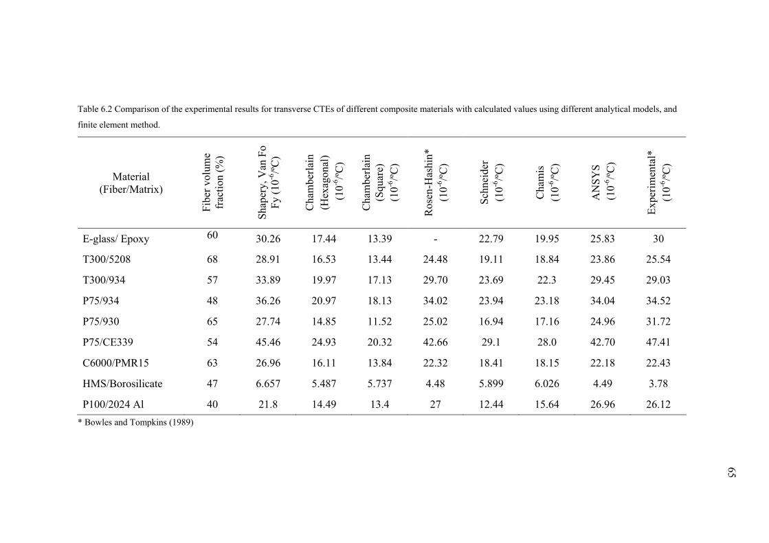
6565
Material (Fiber/Matrix)
Fibe
r vol
ume
frac
tion
(%)
SFy
(10
hape
ry, V
an F
o -6
/ºC)
Cha
mbe
rlain
(H
exag
onal
) (1
0-6/ºC
)
Cha
mbe
rlain
(S
quar
e)
(10-6
/ºC)
Ros
en-H
ashi
n*
(10-6
/ºC)
Schn
eide
r (1
0-6/ºC
)
Cha
mis
(1
0-6/ºC
)
AN
SYS
(10-6
/ºC)
Expe
rimen
tal*
(10-6
/ºC)
E-glass/ Epoxy 60 30.26 17.44 13.39 - 22.79 19.95 25.83 30
T300/5208
68 28.91 16.53 13.44 24.48 19.11 18.84 23.86 25.54
T300/934 57 33.89 19.97 17.13 29.70 23.69 22.3 29.45 29.03
P75/934 48 36.26 20.97 18.13 34.02 23.94 23.18 34.04 34.52
P75/930 65 27.74 14.85 11.52 25.02 16.94 17.16 24.96 31.72
P75/CE339 54 45.46 24.93 20.32 42.66 29.1 28.0 42.70 47.41
C6000/PMR15 63 26.96 16.11 13.84 22.32 18.41 18.15 22.18 22.43
HMS/Borosilicate 47 6.657 5.487 5.737 4.48 5.899 6.026 4.49 3.78
P100/2024 Al 40 21.8 14.49 13.4 27 12.44 15.64 26.96 26.12
Table 6.2 Comparison of the experimental results for transverse CTEs of different composite materials with calculated values using different analytical models, and
finite element method.
* Bowles and Tompkins (1989)
66
0.00E+00
2.50E-06
5.00E-06
7.50E-06
1.00E-05
1.25E-05
1.50E-05
1.75E-05
2.00E-05
2.25E-05
0 0.1 0.2 0.3 0.4 0.5 0.6 0.7 0.8 0.9 1
Fiber volume fraction
Long
itudi
nal C
TE (
1/°C
)
Shapery, Van Fo Fy,Chamis
Schneider, Chamberlain
ANSYS
Experimental (Sideridis, 1994)
Figure 6.1 Longitudinal CTE of E-Glass/Epoxy composite.
0.00E+00
1.00E-05
2.00E-05
3.00E-05
4.00E-05
5.00E-05
6.00E-05
7.00E-05
0.0 0.1 0.2 0.3 0.4 0.5 0.6 0.7 0.8 0.9 1.0
Fiber volume fraction
Tran
sver
se C
TE (
1/°C
)
Law of mixtures
Shapery, Van Fo Fy
Chamberlain (Hex)
Chamberlain (Sq)
Chamis
Schneider
ANSYS
Experimental (Sideridis, 1994)
Figure 6.2 Transverse CTE of E-Glass/Epoxy composite.

67
-1.00E-06
0.00E+00
1.00E-06
2.00E-06
3.00E-06
4.00E-06
5.00E-06
6.00E-06
7.00E-06
0 0.1 0.2 0.3 0.4 0.5 0.6 0.7 0.8 0.9 1
Fiber volume fraction
Long
itudi
nal C
TE (1
/°C
)
Shapery, Van Fo Fy,ChamisSchneider, ChamberlainANSYSExperimental (T300/5208)Experimental (T300/934)
Figure 6.3 Longitudinal CTE of T300/5208, and T300/934 composites.
0.00E+00
1.00E-05
2.00E-05
3.00E-05
4.00E-05
5.00E-05
6.00E-05
7.00E-05
0.0 0.1 0.2 0.3 0.4 0.5 0.6 0.7 0.8 0.9 1.0
Fiber volume fraction
Tran
sver
e C
TE (1
/°C
)
Law of mixtures
Shapery, Van Fo Fy
Chamberlain (Hex)
Chamberlain (Sq)
Chamis
ANSYS
Schneider
Experimental (T300/5208)
Experimental (T300/934)
Figure 6.4 Transverse CTE of T300/5208, and T300/934 composites.
68
-2.00E-06
-1.50E-06
-1.00E-06
-5.00E-07
0.00E+00
5.00E-07
1.00E-06
1.50E-06
2.00E-06
0 0.1 0.2 0.3 0.4 0.5 0.6 0.7 0.8 0.9 1
Fiber volume fraction
Long
itudi
nal C
TE (1
/°C
)
Shapery, Van Fo Fy,ChamisSchneider, ChamberlainANSYSExperimental (P75/934)Experimental (P75/930)
Figure 6.5 Longitudinal CTE of P75/934, and P75/930 composites.
0.00E+00
1.00E-05
2.00E-05
3.00E-05
4.00E-05
5.00E-05
6.00E-05
0.0 0.1 0.2 0.3 0.4 0.5 0.6 0.7 0.8 0.9 1.0
Fiber volume fraction
Tran
sver
se C
TE (1
/°C
)
Law of mixtures
Shapery, Van Fo Fy
Chamberlain (Hex)
Chamberlain (Sq)
Chamis
ANSYS
Schneider
Experimental (P75/934)
Experimental (P75/930)
Figure 6.6 Transverse CTE of P75/934, and P75/930 composites.
69
-2.00E-06
-1.00E-06
0.00E+00
1.00E-06
2.00E-06
3.00E-06
4.00E-06
0 0.1 0.2 0.3 0.4 0.5 0.6 0.7 0.8 0.9 1
Fiber volume fraction
Long
itudi
nal C
TE (1
/°C
)
Shapery, Van Fo Fy,Chamis
Schneider, Chamberlain
ANSYSExperimental
Figure 6.7 Longitudinal CTE of P75/CE339 composite.
0.00E+00
1.00E-05
2.00E-05
3.00E-05
4.00E-05
5.00E-05
6.00E-05
7.00E-05
8.00E-05
0.0 0.1 0.2 0.3 0.4 0.5 0.6 0.7 0.8 0.9 1.0
Fiber volume fraction
Tran
sver
se C
TE (1
/°C
)
Law of mixtures
Shapery, Van Fo Fy
Chamberlain (Hex)
Chamberlain (Sq)
Chamis
ANSYS
Schneider
Experimental
Figure 6.8 Transverse CTE of P75/CE339 composite.

70
-1.00E-06
0.00E+00
1.00E-06
2.00E-06
3.00E-06
4.00E-06
0 0.1 0.2 0.3 0.4 0.5 0.6 0.7 0.8 0.9 1
Fiber volume fraction
Long
itudi
nal C
TE (1
/°C
) Shapery, Van Fo Fy,Chamis
Schneider, Chamberlain
ANSYSExperimental
Figure 6.9 Longitudinal CTE of C6000/PMR15 composite.
0.00E+00
1.00E-05
2.00E-05
3.00E-05
4.00E-05
5.00E-05
0.0 0.1 0.2 0.3 0.4 0.5 0.6 0.7 0.8 0.9 1.0
Fiber volume fraction
Tran
sver
se C
TE (1
/°C
)
Law of mixtures
Shapery, Van Fo Fy
Chamberlain (Hex)
Chamberlain (Sq)
Chamis
ANSYS
Schneider
Experimental
Figure 6.10 Transverse CTE of C6000/PMR15 composite.
71
-1.00E-06
-5.00E-07
0.00E+00
5.00E-07
1.00E-06
1.50E-06
2.00E-06
0 0.1 0.2 0.3 0.4 0.5 0.6 0.7 0.8 0.9 1
Fiber volume fraction
Long
itudi
nal C
TE (1
/°C
)
Shapery, Van Fo Fy,Chamis,Schneider, Chamberlain
ANSYS
Experimental
Figure 6.11 Longitudinal CTE of HMS/BG composite.
3.00E-06
4.00E-06
5.00E-06
6.00E-06
7.00E-06
8.00E-06
9.00E-06
1.00E-05
0.0 0.1 0.2 0.3 0.4 0.5 0.6 0.7 0.8 0.9 1.0
Fiber volume fraction
Tran
sver
se C
TE (1
/°C
)
Law of mixtures
Shapery, Van Fo Fy
Chamberlain (Hex)
Chamberlain (Sq)
Chamis
ANSYS
Schneider
Experimental
Figure 6.12 Transverse CTE of HMS/BG composite.

72
-2.00E-06
0.00E+00
2.00E-06
4.00E-06
6.00E-06
8.00E-06
1.00E-05
0 0.1 0.2 0.3 0.4 0.5 0.6 0.7 0.8 0.9 1
Fiber volume fraction
Long
itudi
nal C
TE (1
/°C
) Shapery, Van Fo Fy,Chamis
Schneider, Chamberlain
ANSYSExperimental
Figure 6.13 Longitudinal CTE of P100/2024Al composite.
0.00E+00
5.00E-06
1.00E-05
1.50E-05
2.00E-05
2.50E-05
3.00E-05
0.0 0.1 0.2 0.3 0.4 0.5 0.6 0.7 0.8 0.9 1.0
Fiber volume fraction
Tran
sver
se C
TE (1
/°C
)
Law of mixturesShapery, Van Fo Fy
Chamberlain (Hex)Chamberlain (Sq)
ChamisANSYS
SchneiderExperimental
Figure 6.14 Transverse CTE of P100/2024Al composite.

73
REFERENCES
Adams, D.F., & Crane D.A. (1984). Combined loading micromechanical analysis of
a unidirectional composite. Composites, 15 (3), 181-192.
Bowles, D.E., & Tompkins S.S. (1989). Prediction of coefficients of thermal
expansion for unidirectional composites. Journal of Composite Materials, 23,
370-388.
Callister, W.D. (1994). Materials science and engineering; an introduction (3rd ed.).
New York: John Wiley & Sons, Inc.
Chamis, C.C., & Sendecky G.P. (1968). Critique on theories predicting thermoelastic
properties of fibrous composites. Journal of Composite Materials, 2 (3), 332-358.
Chandrupatla, T.R., & Belegundu A.D. (2002). Introduction to Finite Elements in
Engineering (3rd ed.). New Jersey: Prentice Hall.
Chawla, K.K. (1998). Composite materials science and engineering (2nd ed.). New
York: Springer-Verlag.
Foye, R.L. (1968). Advanced design concepts for advanced composite airframes.
Technical Report AFML-TR-68-91. Columbus: North American-Rockwell
Corporation.
Hashin, Z. (1979). Analysis of properties of fiber composites with anisotropic
constituents. Journal of Applied Mechanics, 46, 543-550.
Hill, R. (1964). Theory of mechanical properties of fibre-strengthened materials: 1.
elastic behavior. Journal of the Mechanics and Physics of Solids, 12 (4), 199-
212.
IARC, 1988. Man-made Fibers and Radon. IARC Monographs on the Evaluation of
Carcinogenic Risk of Chemicals to Humans, 43. 300.

74
Ishikava, T., Koyama, K., & Kobayashi, S. (1978). Thermal expansion coefficients
of unidirectional composites. Journal of Composite Materials, 12, 153-168.
Islam, MD.R., Sjölind, S.G., & Pramila A. (2001). Finite element analysis of linear
thermal expansion coefficients of unidirectional cracked composites. Journal of
Composite Materials, 35, 1762-1776.
Johnson, R.R., Kural M.H., & Mackey G.B. (1981) Thermal expansion properties of
composite materials. California: Lockheed Missiles and Space Co. Inc.
Jones, R.M. (1999). Mechanics of composite materials (2nd ed.). Philadelphia:
Taylor and Francis. Levin, V.M. (1967). On the coefficients of thermal expansion of heterogeneous
materials (in Russian). Mekhanika Tverdogo Tela, 88.
Moaveni, S. (1999). Finite element analysis theory and application with ANSYS.
New Jersey: Prentice Hall.
Morrell, R. (1997). Thermal property measurement and data on composite materials.
Measurement Note CMMT(MN)011. London: National Physical Laboratory.
Rogers, K.F., Phillips, L.N., Kingston-Lee, D.M., Yates, B., Overy M.J., Sargent,
J.P., et al. (1977).The thermal expansion of carbon fibre-reinforced plastics.
Journal of Materials Science, 12, 718-734.
Rosen, B.W. & Hashin, Z. (1970). Effective thermal expansion coefficients and
specific heats of composite materials. International Journal of Engineering
Science, 8, 157-173.
Rupnowski, P., Gentza, M., Sutterb, J.K., & Kumosa M. (2005). An evaluation on
the elastic properties and thermal expansion coefficients of medium and high
modulus graphite fibers. Composites: Part A, 36 (3), 327-338
Schapery, R.A. (1968). Thermal expansion coefficients of composite materials based
on energy principles. Journal of Composite Materials, 2 (3), 380-404.

75
Shen, Y.L. (1998). Thermal Expansion of Metal-Ceramic Composites: A Three
Dimensional Analysis. Materials Science and Engineering A, 252, 269-275.
Sideridis, E. (1994). Thermal expansion coefficient of fiber composites defined by
the concept of the interphase. Composites Science and Technology, 51, 301-317.
Technical note 69: Principles of Push-Rod Dilatometry, (n.d.). Retrieved July 11,
2005 from http://www.anter.com/TN69.htm
Thermal expansion (n.d) Retrieved July 11, 2005 from
http://www.pmiclab.com/testing/ThermalExpansion.html
Tantina, G., Nimmer, R., (1994). Structural analysis of thermoplastic components.
Malnati P. (Ed.). New York: McGraw-Hill, Inc.
Tsai, S.W., & Hahn, H. T. (1980). Introduction to composite materials. Lancester:
Technomic Publishing Co. Inc.
Wypych G. (2000). Handbook of fillers (2nd ed.). Toronto: ChemTec Publishing.
Van Fo Fy, G. A. (1965). Thermal strains and stresses in glass fiber reinforced media
(in Russian). Prikl. Mekh. Teor. Fiz., 101.
Van Fo Fy, G. A., & Savin G. N. (1965). Fundamentals of the theory of non-fabric
glass reinforced plastics (in Russian). Mekhanika Polimerov, 1, 151.
Van Fo Fy, G. A. (1966). Elastic constants and thermal expansion of certain bodies
with inhomogeneous regular structure (in Russian). Soviet Physics, Doklady, 11,
176.
Van Fo Fy, G. A. (1966). Basic relations of the theory of oriented glass reinforced
plastics with hollow fibers (in Russian). Mekhanika Polimerov, 2, 763.