A P-ADAPTIVE IMPLICIT DISCONTINUOUS GALERKIN … · Key words: Discontinuous Galerkin methods, p-adaptation, Compressible ILES ... In the last decades Computational Fluid Dynamics

6th European Conference on Computational Mechanics (ECCM 6)7th European Conference on Computational Fluid Dynamics (ECFD 7)

11-15 June 2018, Glasgow, UK

A P-ADAPTIVE IMPLICIT DISCONTINUOUS GALERKINMETHOD FOR THE UNDER-RESOLVED SIMULATION OF

COMPRESSIBLE TURBULENT FLOWS

A. Colombo1, G. Manzinali1, A. Ghidoni2, G. Noventa2,M. Franciolini3, A. Crivellini3 and F. Bassi1

1 University of Bergamo, Department of Engineering and Applied Sciences, viale Marconi, 5 -24044 Dalmine (BG), Italy, alessandro.colombo, [email protected],

[email protected]

2 University of Brescia, Department of Mechanical and Industrial Engineering, via Branze, 38 -25123, Brescia, Italy, antonio.ghidoni, [email protected]

3 Marche Polytechnic University, Department of Industrial Engineering and MathematicalScience, via Brecce Bianche, 12 - 60131 Ancona, Italy,

[email protected], [email protected]

Key words: Discontinuous Galerkin methods, p-adaptation, Compressible ILES

Abstract. In the last decades Computational Fluid Dynamics has become a widespreadpractice in several industrial fields, e.g., aerodynamics, aeroacoustic. The growing need ofhigh-fidelity flow simulations for the accurate determination of problem-specific quantitiespaved the way to higher-order methods such as the discontinuous Galerkin (DG) method.In this context, the industrial interest is strongly promoting the development of moreand more efficient high-order CFD solvers. In this work we exploit some techniques, i.e.p-adaptation, quadrature reduction and load balancing, to enhance the computationalefficiency of an existing DG code. The accuracy and efficiency of our approach will beassessed by computing the implicit Large Eddy Simulation of the flow past a circularcylinder at Reynolds number Re = 3900, and around a NACA0018 airfoil at Reynoldsnumber Re = 10000 and angle of attack α = 15.

1 INTRODUCTION

In the last decades Computational Fluid Dynamics (CFD) has become a widespreadpractice in several industrial fields, e.g. aerodynamics, aeroacoustic, turbomachinery. Thegrowing need of high-fidelity flow simulations for the accurate determination of problem-specific quantities paved the way to higher-order methods such as the DiscontinuousGalerkin (DG) methods. DG methods, if compared to standard industrial code, showsome deficiency in terms of computational efficiency. However, the industrial interest isstrongly promoting research efforts to devise more efficient high-order CFD solvers. The

A. Colombo, G. Manzinali, A. Ghidoni, G. Noventa, M. Franciolini, A. Crivellini and F. Bassi

aim of this paper is to describe an approach to enhance the computational efficiency of anexisting DG code [1], based on p-adaptation, quadrature reduction and load balancing.

A p-adaptation strategy that allows the variation of the polynomial degree of thesolution between the elements is adopted, obtaining a sensible reduction of the simulationCPU time and memory, while not spoiling at all the high accuracy required by this class ofsimulations. In particular, being interested in unsteady flows computations, such as DirectNumerical Simulation (DNS) and Large Eddy Simulation (LES), we will investigate anadaptation procedure suitable for time-dependent problems. Adaptation is here drivenby two simple indicators, based on interface pressure jumps and on the decay of thecoefficients of the modal expansion. These sensors are coupled to guarantee a reasonablebehaviour both for high- and low-degree polynomial approximations. Moreover, the degreeof exactness of quadrature rules is adapted on the computational domain to avoid overintegration of straight sided elements, and runtime load-balancing is applied, based on theMetis library capability to generate “weighted” graphs, to handle the degrees of freedomunbalance on each partition due to the adaptation algorithm.

The robustness and efficiency of the proposed approach is evaluated by computing theILES of the flow past a circular cylinder at Reynolds number Re = 3900, and around aNACA0018 airfoil at Reynolds number Re = 10000 and angle of attack α = 15.

In Section 2 we briefly introduce the DG space and the time discretizations. Section 3describes the definition of orthonormal hierarchical polynomial basis and the possibleapproaches to their evaluation, while Section 4 the error estimators used to drive theadaptaton. Sections 5 and 6 describe the techniques adopted to adapt the degree ofexactness of the quadrature rules and to balance the load of each processor. Finally, inSection 7 a strategy for the p-adaptation is proposed and applied to different unsteadycompressible test cases.

2 THE NUMERICAL FRAMEWORK

The Navier-Stokes equations for the m variables in d dimensions can be written incompact form as

P(w)∂w

∂t+∇ · Fc(w) +∇ · Fv(w,∇w) = 0, (1)

where w ∈ Rm is the unknown solution vector, Fc,Fv ∈ Rm ⊗ Rd are the convective andviscous flux functions, and P (w) ∈ Rm ⊗ Rm is a transformation matrix. Employingthe conservative variables wc = [ρ, ρui, ρE]T for compressible flows P reduces to theidentity matrix (P = I). By multiplying Eq. (1) by an arbitrary smooth test functionv = v1, . . . , vm, and integrating by parts, we obtain the weak formulation∫

Ω

v ·(P (w)

∂w

∂t

)dx−

∫Ω

∇v : F (w,∇w) dx +

∫∂Ω

v ⊗ n : F (w,∇w) dσ = 0, (2)

where F is the sum of the convective and viscous flux functions and n is the unit vectornormal to the boundary.

To discretize Eq. (2) we replace the solution w and the test function v with a finiteelement approximation wh and a discrete test function vh, respectively, where wh and vh

2


belong to the space Vhdef= [Pk

d(Th)]m. Pkd(T ) denotes the restriction to non overlapping

arbitrary shaped mesh elements T ∈ Th of the polynomial functions of d variables andtotal degree ≤ k. For each of the m equations of system (2), and without loss of generality,we choose the set of test and shape functions in any element T coincident with the set oforthogonal and hierachical basis functions in that element. The DG discretization of theviscous fluxes is based on the BR2 scheme, proposed in [2], while the convective numericalflux is computed from the solution of local Riemann problems in the normal direction ateach quadrature point on elements faces.

By assembling together all the elemental contributions of the DG discretization, thesystem of Ordinary Differential Equations (ODEs) governing the evolution in time of thediscrete solution can be written as

dW

dt= R (W) , (3)

withR (W) = M−1 (W)R (W) , (4)

where W is the global vector of unknown degrees of freedom, M is the global blockdiagonal mass matrix, and R (W) is the vector of residuals. In this work we integrate intime by using the linearly implicit (Rosenbrock-type) Runge-Kutta schemes [3].

3 EFFICIENT EVALUATION OF THE BASIS FUNCTIONS

In this section we briefly describe the approach proposed in [4] to build a set of or-

thonormal and hierarchical basis functions. Let ΦkT =

φTi

i∈1,...,NT

dofdenote an initial

set of monomials defined in a reference frame relocated in the element barycentre andaligned with the principal axes of inertia of T . To obtain a new set of orthonormal basisfunctions, Φk

T =φTi

i∈1,...,NT

dof, we apply Algorithm 1 (modified Gram-Schmidt proce-

dure, MGS) for all T ∈ Th, where(φTi , φ

Tj

)T

is the evaluation of the inner product, rTii

and rTij the coefficients of the MGS algorithm.

Algorithm 1 Modified Gram-Schmidt orthogonalization algorithm

1: for i = 1 to NTdof do

2: for i = 1 to NTdof do

3: rTij ←(φTi , φ

Tj

)T

4: φTi ← φT

i − rTijφTj remove the projection of φT

i onto φTj

5: end for

6: rTii ←√(

φTi , φ

Tj

)T

7: φTi ← φT

i /rTii normalize

8: φTi ← φT

i

9: end for

3


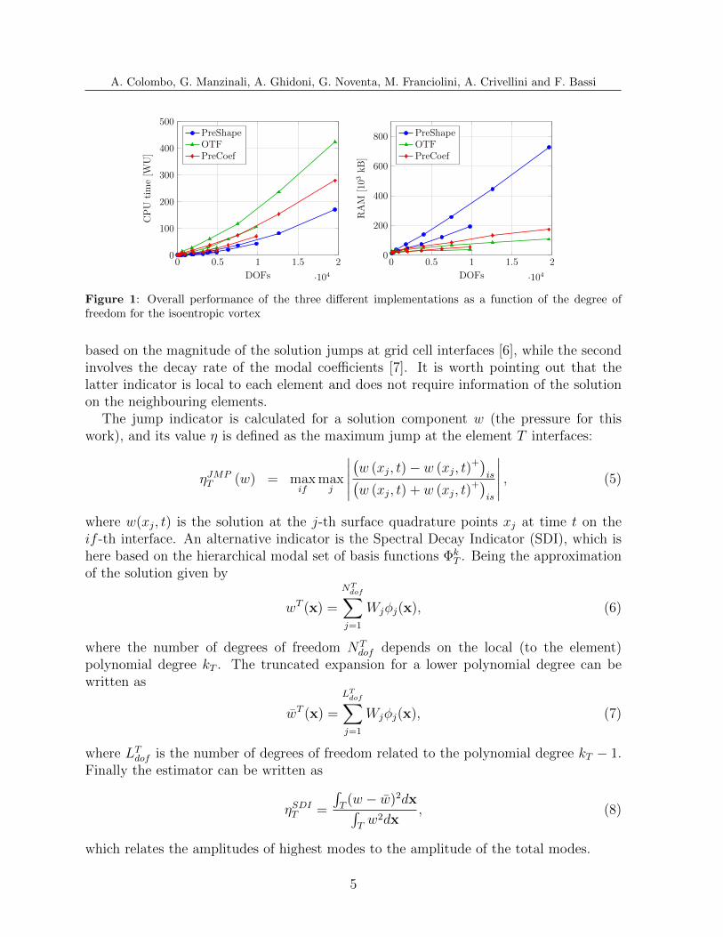
The basis functions can be evaluated following three different strategies, characterizedby different computational cost and memory:

• Full storing (PreShape). For each element and face the basis functions and, ifneeded, their derivatives are evaluated at each Gauss point, during pre-processingand stored in memory.

• Orthonormalization coefficients storing (PreCoef). The monomials evaluation, theirorthonormalization and the computation of the orthonormalization coefficients areperformed separately. The coefficients are evaluated and stored during pre-processingfor each element, according to the corresponding polynomial degree. Then, themonomials are evaluated on-the-fly and orthonormalized, using the pre-computedcoefficients.

• On-the-fly evaluation (OTF). There is no storage related to the basis evaluation,and both the monomials and the orthonormalization coefficients are re-computedon-the-fly.

The test cases employed to compare the performance of the three proposed implementa-tion was the transport of a vortex in uniform flow, both with Euler and Navier–Stokesequations. In the latter case, the Reynolds number was Re = 100. In this section wefocus only on the efficiency of the solver rather than considering the temporal accuracy.Three different meshes, respectively made of 252, 502, and 1002 quadrilateral elementswith linear edges, were considered.

Fig. 1 shows the performance comparison, in terms of CPU time and memory, regardingthe computation of the inviscid test case for the three strategies as a function of the totalnumber of degrees of freedom. The computational time is given in terms of Work Units(WU) defined as WU = tsnc/τb, where ts is the measured CPU time of a simulation onnc cores and τb is the reference TauBench time of the hardware1. According to this study,the PreCoef strategy seems to be an a appealing compromise between CPU time and thememory footprint, and, therefore, it will be used for the development of our p-adaptationstrategy. In particular we pre-compute the orthonormalization coefficients correspondingto the maximum polynomial degree allowed by the user defined adaptation parameters,here fixed at k = 6, and use them to orthonormalize monomials according to the local(elemental) polynomial degree of the solution on-the-fly. Same trends have been obtainedfor the viscous vortex.

4 A p-ADAPTATION STRATEGY

The adaptation is driven by error estimators that control the solution accuracy withinthe domain, identifying the regions lacking/exceeding the requested resolution. In thiswork these regions will be refined/coarsened by increasing/decreasing the degree of thepolynomial approximation of the solution. Among the several alternatives proposed inliterature for DG schemes, we rely on the combination of two indicators. The first one is

1-n 250000 -s 10 define the reference TauBench workload for the hardware benchmark

4


0 0.5 1 1.5 2

·104

0

100

200

300

400

500

DOFs

CP

Uti

me

[WU

]

PreShapeOTFPreCoef

0 0.5 1 1.5 2

·104

0

200

400

600

800

DOFs

RA

M[1

03kB

]

PreShapeOTFPreCoef

Figure 1: Overall performance of the three different implementations as a function of the degree offreedom for the isoentropic vortex

based on the magnitude of the solution jumps at grid cell interfaces [6], while the secondinvolves the decay rate of the modal coefficients [7]. It is worth pointing out that thelatter indicator is local to each element and does not require information of the solutionon the neighbouring elements.

The jump indicator is calculated for a solution component w (the pressure for thiswork), and its value η is defined as the maximum jump at the element T interfaces:

ηJMPT (w) = max

ifmax

j

∣∣∣∣∣(w (xj, t)− w (xj, t)

+)is(

w (xj, t) + w (xj, t)+)

is

∣∣∣∣∣ , (5)

where w(xj, t) is the solution at the j-th surface quadrature points xj at time t on theif -th interface. An alternative indicator is the Spectral Decay Indicator (SDI), which ishere based on the hierarchical modal set of basis functions Φk

T . Being the approximationof the solution given by

wT (x) =

NTdof∑

j=1

Wjφj(x), (6)

where the number of degrees of freedom NTdof depends on the local (to the element)

polynomial degree kT . The truncated expansion for a lower polynomial degree can bewritten as

wT (x) =

LTdof∑

j=1

Wjφj(x), (7)

where LTdof is the number of degrees of freedom related to the polynomial degree kT − 1.

Finally the estimator can be written as

ηSDIT =

∫T

(w − w)2dx∫Tw2dx

, (8)

which relates the amplitudes of highest modes to the amplitude of the total modes.

5


Numerical experiments on the vortex test case show that the former indicator is reliablefor any polynomial degree, whereas the latter gives reasonable indications only for k ≥ 2,assuming unit valure over the whole computation domain for lower degrees. MoreoverηJMP is more diffusive, identifying a larger region for adaptation. According to theseobservations, we implemented a combination of the two indicators

ηTOTT = ηSDI

T INT

(kT

max(2, kT )

)+

1

max (1, kT )ηJMPT ∀T ∈ Th, (9)

where INT represent an integer division (ηSDIT is set to 0 for kT = 0, 1). Before the

coupling both indicators are normalized over the domain according to their maximum andminimum values.

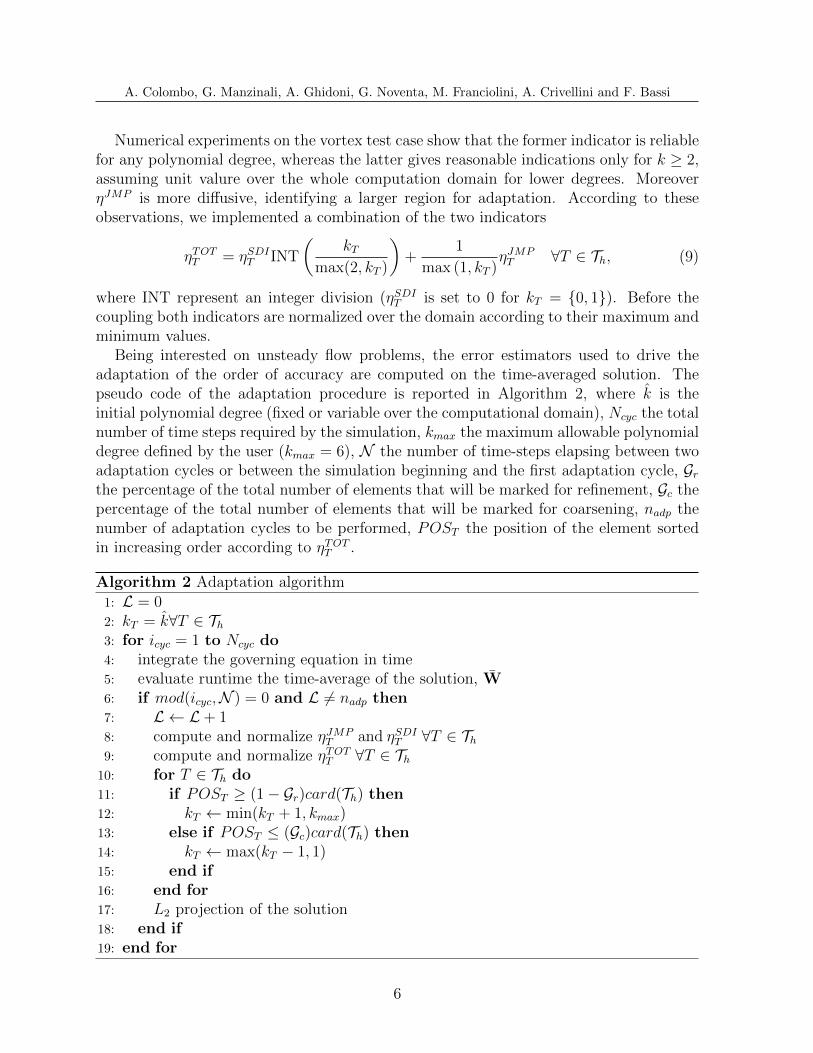
Being interested on unsteady flow problems, the error estimators used to drive theadaptation of the order of accuracy are computed on the time-averaged solution. Thepseudo code of the adaptation procedure is reported in Algorithm 2, where k is theinitial polynomial degree (fixed or variable over the computational domain), Ncyc the totalnumber of time steps required by the simulation, kmax the maximum allowable polynomialdegree defined by the user (kmax = 6), N the number of time-steps elapsing between twoadaptation cycles or between the simulation beginning and the first adaptation cycle, Grthe percentage of the total number of elements that will be marked for refinement, Gc thepercentage of the total number of elements that will be marked for coarsening, nadp thenumber of adaptation cycles to be performed, POST the position of the element sortedin increasing order according to ηTOT

T .

Algorithm 2 Adaptation algorithm1: L = 02: kT = k∀T ∈ Th3: for icyc = 1 to Ncyc do4: integrate the governing equation in time5: evaluate runtime the time-average of the solution, W6: if mod(icyc,N ) = 0 and L 6= nadp then7: L ← L+ 18: compute and normalize ηJMP

T and ηSDIT ∀T ∈ Th

9: compute and normalize ηTOTT ∀T ∈ Th

10: for T ∈ Th do11: if POST ≥ (1− Gr)card(Th) then12: kT ← min(kT + 1, kmax)13: else if POST ≤ (Gc)card(Th) then14: kT ← max(kT − 1, 1)15: end if16: end for17: L2 projection of the solution18: end if19: end for

6


Orthonormal and herarchical modal bases simplify the L2 projection operators. Inpractice, the DOFs of the restricted solution are equal to the low-order subset of theirhigh-order representations, while the DOFs of the prolongated solution are the same asthe low-order solution with null high-order components.

5 REDUCED QUADRATURES

The number of quadrature points rapidly increases when considering high order poly-nomials and curved elements. However, as demonstrated in [4], not always the exactquadrature is necessary to maintain the theoretical order of accuracy. To identify onlythe regions of the mesh that require full quadrature points, we introduce the followingmeasure for the integration error on the element T :

εi,T = |m∗ii −mexii | ∀T ∈ Th, (10)

where m∗ii denotes the value of the i-th diagonal entry of the local mass matrix computedwith the reduced quadrature rule, whereas mex

ii is the expected value as a result of exactintegration. Then we use on the elements of Th an integration rule with the minimumdegree of exactness needed to satisfy the condition:

maxi∈1,...,NT

dofεi,T ≤ tol, ∀T ∈ Th, (11)

where tol is a user-defined tolerance in the diagonal entries of the mass matrix.

6 LOAD BALANCING

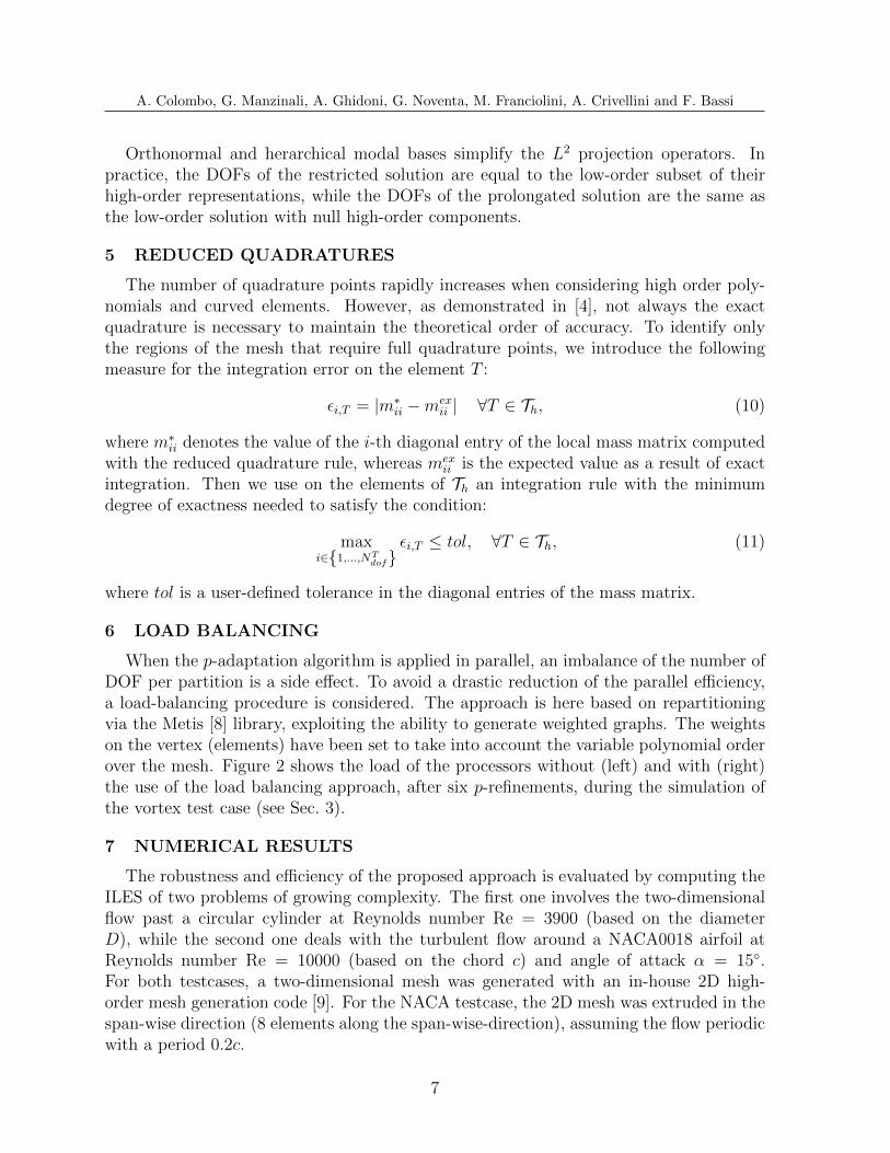
When the p-adaptation algorithm is applied in parallel, an imbalance of the number ofDOF per partition is a side effect. To avoid a drastic reduction of the parallel efficiency,a load-balancing procedure is considered. The approach is here based on repartitioningvia the Metis [8] library, exploiting the ability to generate weighted graphs. The weightson the vertex (elements) have been set to take into account the variable polynomial orderover the mesh. Figure 2 shows the load of the processors without (left) and with (right)the use of the load balancing approach, after six p-refinements, during the simulation ofthe vortex test case (see Sec. 3).

7 NUMERICAL RESULTS

The robustness and efficiency of the proposed approach is evaluated by computing theILES of two problems of growing complexity. The first one involves the two-dimensionalflow past a circular cylinder at Reynolds number Re = 3900 (based on the diameterD), while the second one deals with the turbulent flow around a NACA0018 airfoil atReynolds number Re = 10000 (based on the chord c) and angle of attack α = 15.For both testcases, a two-dimensional mesh was generated with an in-house 2D high-order mesh generation code [9]. For the NACA testcase, the 2D mesh was extruded in thespan-wise direction (8 elements along the span-wise-direction), assuming the flow periodicwith a period 0.2c.

7


5 10 15 20 25 30 35 40 450

500

1,000

1,500

process id

DO

Fs

0th1th adap.2th adap.3th adap.4th adap.5th adap.6th adap.

5 10 15 20 25 30 35 40 450

500

1,000

1,500

process id

DO

Fs

0th1th adap.2th adap.3th adap.4th adap.5th adap.6th adap.

Figure 2: Load of the processors without (top) and with (bottom) the use of the load balancing approachafter six p-refinements, invicid isoentropic vortex

7.1 FLOW PAST A CIRCULAR CYLINDER

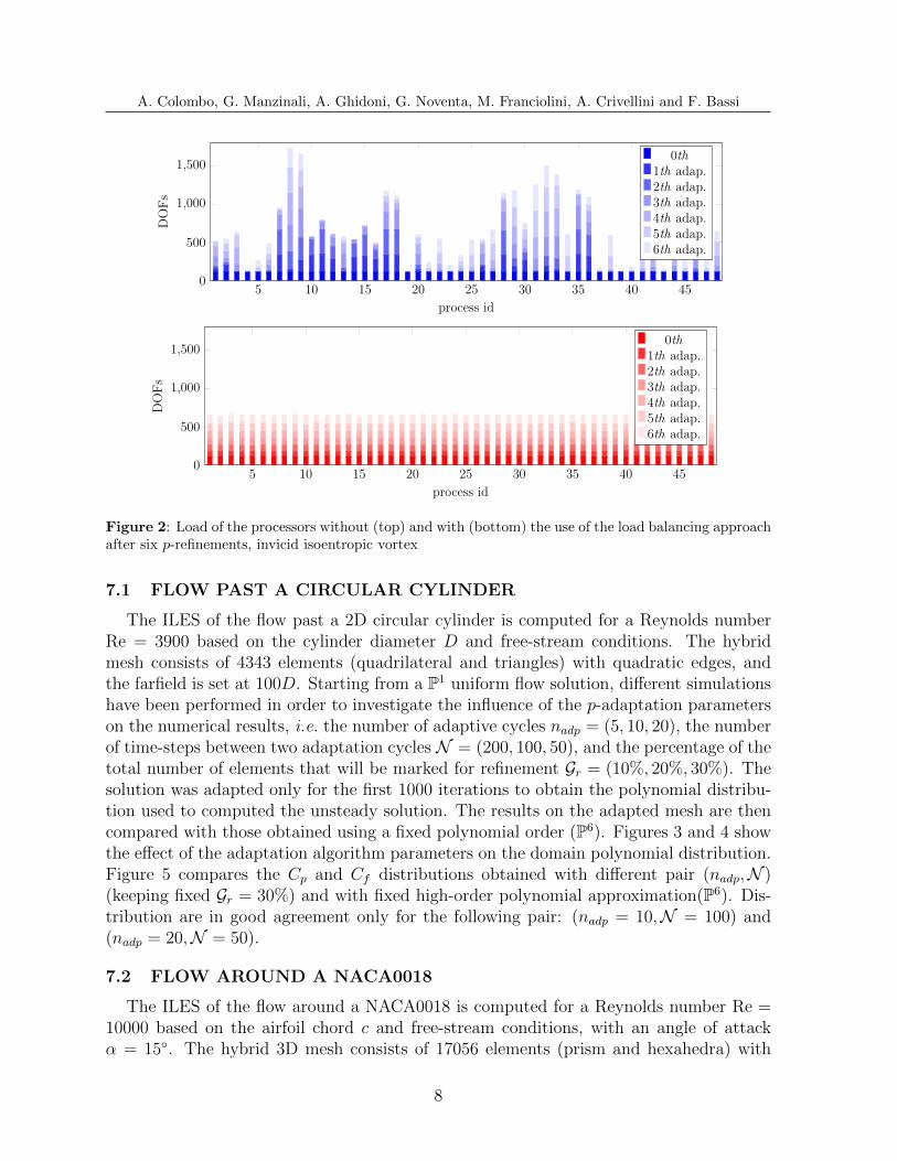
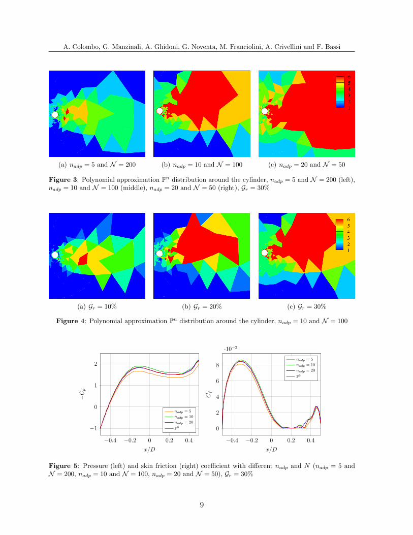
The ILES of the flow past a 2D circular cylinder is computed for a Reynolds numberRe = 3900 based on the cylinder diameter D and free-stream conditions. The hybridmesh consists of 4343 elements (quadrilateral and triangles) with quadratic edges, andthe farfield is set at 100D. Starting from a P1 uniform flow solution, different simulationshave been performed in order to investigate the influence of the p-adaptation parameterson the numerical results, i.e. the number of adaptive cycles nadp = (5, 10, 20), the numberof time-steps between two adaptation cycles N = (200, 100, 50), and the percentage of thetotal number of elements that will be marked for refinement Gr = (10%, 20%, 30%). Thesolution was adapted only for the first 1000 iterations to obtain the polynomial distribu-tion used to computed the unsteady solution. The results on the adapted mesh are thencompared with those obtained using a fixed polynomial order (P6). Figures 3 and 4 showthe effect of the adaptation algorithm parameters on the domain polynomial distribution.Figure 5 compares the Cp and Cf distributions obtained with different pair (nadp,N )(keeping fixed Gr = 30%) and with fixed high-order polynomial approximation(P6). Dis-tribution are in good agreement only for the following pair: (nadp = 10,N = 100) and(nadp = 20,N = 50).

7.2 FLOW AROUND A NACA0018

The ILES of the flow around a NACA0018 is computed for a Reynolds number Re =10000 based on the airfoil chord c and free-stream conditions, with an angle of attackα = 15. The hybrid 3D mesh consists of 17056 elements (prism and hexahedra) with

8


(a) nadp = 5 and N = 200 (b) nadp = 10 and N = 100 (c) nadp = 20 and N = 50

Figure 3: Polynomial approximation Pn distribution around the cylinder, nadp = 5 and N = 200 (left),nadp = 10 and N = 100 (middle), nadp = 20 and N = 50 (right), Gr = 30%

(a) Gr = 10% (b) Gr = 20% (c) Gr = 30%

Figure 4: Polynomial approximation Pn distribution around the cylinder, nadp = 10 and N = 100

−0.4 −0.2 0 0.2 0.4

−1

0

1

2

x/D

−C

p

nadp = 5

nadp = 10

nadp = 20

P6

−0.4 −0.2 0 0.2 0.4

0

2

4

6

8

·10−2

x/D

Cf

nadp = 5

nadp = 10

nadp = 20

P6

Figure 5: Pressure (left) and skin friction (right) coefficient with different nadp and N (nadp = 5 andN = 200, nadp = 10 and N = 100, nadp = 20 and N = 50), Gr = 30%

9


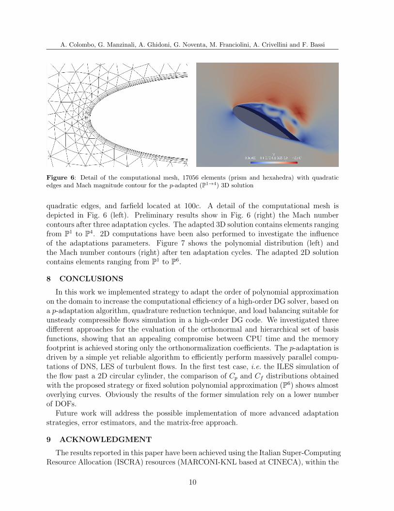
Figure 6: Detail of the computational mesh, 17056 elements (prism and hexahedra) with quadraticedges and Mach magnitude contour for the p-adapted (P1→4) 3D solution

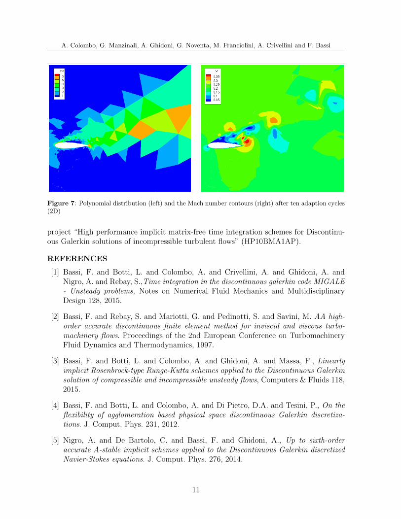
quadratic edges, and farfield located at 100c. A detail of the computational mesh isdepicted in Fig. 6 (left). Preliminary results show in Fig. 6 (right) the Mach numbercontours after three adaptation cycles. The adapted 3D solution contains elements rangingfrom P1 to P4. 2D computations have been also performed to investigate the influenceof the adaptations parameters. Figure 7 shows the polynomial distribution (left) andthe Mach number contours (right) after ten adaptation cycles. The adapted 2D solutioncontains elements ranging from P1 to P6.

8 CONCLUSIONS

In this work we implemented strategy to adapt the order of polynomial approximationon the domain to increase the computational efficiency of a high-order DG solver, based ona p-adaptation algorithm, quadrature reduction technique, and load balancing suitable forunsteady compressible flows simulation in a high-order DG code. We investigated threedifferent approaches for the evaluation of the orthonormal and hierarchical set of basisfunctions, showing that an appealing compromise between CPU time and the memoryfootprint is achieved storing only the orthonormalization coefficients. The p-adaptation isdriven by a simple yet reliable algorithm to efficiently perform massively parallel compu-tations of DNS, LES of turbulent flows. In the first test case, i.e. the ILES simulation ofthe flow past a 2D circular cylinder, the comparison of Cp and Cf distributions obtainedwith the proposed strategy or fixed solution polynomial approximation (P6) shows almostoverlying curves. Obviously the results of the former simulation rely on a lower numberof DOFs.

Future work will address the possible implementation of more advanced adaptationstrategies, error estimators, and the matrix-free approach.

9 ACKNOWLEDGMENT

The results reported in this paper have been achieved using the Italian Super-ComputingResource Allocation (ISCRA) resources (MARCONI-KNL based at CINECA), within the

10


Figure 7: Polynomial distribution (left) and the Mach number contours (right) after ten adaption cycles(2D)

project “High performance implicit matrix-free time integration schemes for Discontinu-ous Galerkin solutions of incompressible turbulent flows” (HP10BMA1AP).

REFERENCES

[1] Bassi, F. and Botti, L. and Colombo, A. and Crivellini, A. and Ghidoni, A. andNigro, A. and Rebay, S.,Time integration in the discontinuous galerkin code MIGALE- Unsteady problems, Notes on Numerical Fluid Mechanics and MultidisciplinaryDesign 128, 2015.

[2] Bassi, F. and Rebay, S. and Mariotti, G. and Pedinotti, S. and Savini, M. AA high-order accurate discontinuous finite element method for inviscid and viscous turbo-machinery flows. Proceedings of the 2nd European Conference on TurbomachineryFluid Dynamics and Thermodynamics, 1997.

[3] Bassi, F. and Botti, L. and Colombo, A. and Ghidoni, A. and Massa, F., Linearlyimplicit Rosenbrock-type Runge-Kutta schemes applied to the Discontinuous Galerkinsolution of compressible and incompressible unsteady flows, Computers & Fluids 118,2015.

[4] Bassi, F. and Botti, L. and Colombo, A. and Di Pietro, D.A. and Tesini, P., On theflexibility of agglomeration based physical space discontinuous Galerkin discretiza-tions. J. Comput. Phys. 231, 2012.

[5] Nigro, A. and De Bartolo, C. and Bassi, F. and Ghidoni, A., Up to sixth-orderaccurate A-stable implicit schemes applied to the Discontinuous Galerkin discretizedNavier-Stokes equations. J. Comput. Phys. 276, 2014.

11


[6] Krivodonova, L. and Xin, J. and Remacle, J.-F. and Chevaugeon, N. and Flaherty,J.E., Shock detection and limiting with discontinuous Galerkin methods for hyperbolicconservation laws. Applied Numerical Mathematics 48, 2004.

[7] Persson, P.-O. and Peraire, J., Sub-cell shock capturing for discontinuous Galerkinmethods. Collection of Technical Papers - 44th AIAA Aerospace Sciences Meeting 2,2006.

[8] Karypis, G. and Kumar, V., MeTis: Unstructured Graph Partitioning and SparseMatrix Ordering System, Version 5.0. http://www.cs.umn.edu/~metis, 2009.

[9] Ghidoni, A. and Pelizzari, E. and Rebay, S. and Selmin, V., 3D anisotropic un-structured grid generation. International Journal for Numerical Methods in Fluids51, 2006.

12

http://www.cs.umn.edu/~metis

Documents

A P-ADAPTIVE IMPLICIT DISCONTINUOUS GALERKIN … · Key words: Discontinuous Galerkin methods, p-adaptation, Compressible ILES ... In the last decades Computational Fluid Dynamics