A package for survival analysis in R

Terry Therneau

December 1, 2019

Contents

1 Introduction 31.1 History . . . . . . . . . . . . . . . . . . . . . . . . . . . . . . . . . . . . . . . . . 31.2 Survival data . . . . . . . . . . . . . . . . . . . . . . . . . . . . . . . . . . . . . . 41.3 Overview . . . . . . . . . . . . . . . . . . . . . . . . . . . . . . . . . . . . . . . . 61.4 Mathematical Notation . . . . . . . . . . . . . . . . . . . . . . . . . . . . . . . . 7

2 Survival curves 92.1 One event type, one event per subject . . . . . . . . . . . . . . . . . . . . . . . . 92.2 Repeated events . . . . . . . . . . . . . . . . . . . . . . . . . . . . . . . . . . . . 142.3 Competing risks . . . . . . . . . . . . . . . . . . . . . . . . . . . . . . . . . . . . 17

2.3.1 Simple example . . . . . . . . . . . . . . . . . . . . . . . . . . . . . . . . . 172.3.2 Monoclonal gammopathy . . . . . . . . . . . . . . . . . . . . . . . . . . . 202.3.3 Variance . . . . . . . . . . . . . . . . . . . . . . . . . . . . . . . . . . . . . 23

2.4 Multi-state data . . . . . . . . . . . . . . . . . . . . . . . . . . . . . . . . . . . . 232.4.1 Myeloid data . . . . . . . . . . . . . . . . . . . . . . . . . . . . . . . . . . 24

2.5 Influence matrix . . . . . . . . . . . . . . . . . . . . . . . . . . . . . . . . . . . . 372.6 Differences in survival . . . . . . . . . . . . . . . . . . . . . . . . . . . . . . . . . 392.7 State space figures . . . . . . . . . . . . . . . . . . . . . . . . . . . . . . . . . . . 39

2.7.1 Further notes . . . . . . . . . . . . . . . . . . . . . . . . . . . . . . . . . . 41

3 Cox model 423.1 One event type, one event per subject . . . . . . . . . . . . . . . . . . . . . . . . 423.2 Repeating Events . . . . . . . . . . . . . . . . . . . . . . . . . . . . . . . . . . . . 483.3 Competing risks . . . . . . . . . . . . . . . . . . . . . . . . . . . . . . . . . . . . 51

3.3.1 MGUS . . . . . . . . . . . . . . . . . . . . . . . . . . . . . . . . . . . . . . 513.4 Multiple event types and multiple events per subject . . . . . . . . . . . . . . . . 56

3.4.1 Data . . . . . . . . . . . . . . . . . . . . . . . . . . . . . . . . . . . . . . . 563.4.2 Fits . . . . . . . . . . . . . . . . . . . . . . . . . . . . . . . . . . . . . . . 58

3.5 Testing proportional hazards . . . . . . . . . . . . . . . . . . . . . . . . . . . . . 623.5.1 Constructed variables . . . . . . . . . . . . . . . . . . . . . . . . . . . . . 633.5.2 Score tests . . . . . . . . . . . . . . . . . . . . . . . . . . . . . . . . . . . 64

4 Accelerated Failure Time models 68

1

5 Tied event times 695.1 Cox model estimates . . . . . . . . . . . . . . . . . . . . . . . . . . . . . . . . . . 695.2 Cumulative hazard and survival . . . . . . . . . . . . . . . . . . . . . . . . . . . . 725.3 Predicted cumulative hazard and surival from a Cox model . . . . . . . . . . . . 725.4 Multi-state models . . . . . . . . . . . . . . . . . . . . . . . . . . . . . . . . . . . 735.5 Parametric Regression . . . . . . . . . . . . . . . . . . . . . . . . . . . . . . . . . 73

5.5.1 Usage . . . . . . . . . . . . . . . . . . . . . . . . . . . . . . . . . . . . . . 735.5.2 Strata . . . . . . . . . . . . . . . . . . . . . . . . . . . . . . . . . . . . . . 745.5.3 Penalized models . . . . . . . . . . . . . . . . . . . . . . . . . . . . . . . . 755.5.4 Specifying a distribution . . . . . . . . . . . . . . . . . . . . . . . . . . . . 755.5.5 Residuals . . . . . . . . . . . . . . . . . . . . . . . . . . . . . . . . . . . . 775.5.6 Predicted values . . . . . . . . . . . . . . . . . . . . . . . . . . . . . . . . 785.5.7 Fitting the model . . . . . . . . . . . . . . . . . . . . . . . . . . . . . . . . 805.5.8 Derivatives . . . . . . . . . . . . . . . . . . . . . . . . . . . . . . . . . . . 825.5.9 Distributions . . . . . . . . . . . . . . . . . . . . . . . . . . . . . . . . . . 83

A Changes from version 2.44 to 3.1 86A.1 Changes in version 3 . . . . . . . . . . . . . . . . . . . . . . . . . . . . . . . . . . 86A.2 Survfit . . . . . . . . . . . . . . . . . . . . . . . . . . . . . . . . . . . . . . . . . . 87A.3 Coxph . . . . . . . . . . . . . . . . . . . . . . . . . . . . . . . . . . . . . . . . . . 88

2

Chapter 1

Introduction

1.1 History

Work on the survival package began in 1985 in connection with the analysis of medical researchdata, without any realization at the time that the work would become a package. Eventually, thesoftware was placed on the Statlib repository hosted by Carnegie Mellon University. Multipleversion were released in this fashion but I don’t have a list of the dates — version 2 was thefirst to make use of the print method that was introduced in ‘New S’ in 1988, which places thatrelease somewhere in 1989. The library was eventually incorporated directly in S-Plus, and fromthere it became a standard part of R.

I suspect that one of the primary reasons for the package’s success is that all of the functionshave been written to solve real analysis questions that arose from real data sets; theoreticalissues were explored when necessary but they have never played a leading role. As a statisticianin a major medical center, the central focus of my department is to advance medicine; statisticsis a tool to that end. This also highlights one of the deficiencies of the package: if a particularanalysis question has not yet arisen in one of my studies then the survival package will also havenothing to say on the topic. Luckily, there are many other R packages that build on or extendthe survival package, and anyone working in the field (the author included) can expect to usemore packages than just this one. The author certainly never foresaw that the library wouldbecome as popular as it has.

This vignette is an introduction to version 3.x of the survival package. We can think ofversions 1.x as the S-Plus era and 2.1 – 2.44 as maturation of the package in R. Version 3 had 4major goals.

� Make multi-state curves and models as easy to use as an ordinary Kaplan-Meier and Coxmodel.

� Deeper support for absolute risk estimates.

� Consistent use of robust variance estimates.

� Clean up various naming inconsistencies that have arisen over time.

3

With over 600 dependent packages in 2019, not counting Bioconductor, other guiding lightsof the change are

� We can’t do everything (so don’t try).

� Allow other packages to build on this one. That means clear documentation of all of theresults that are produced, the use of simple S3 objects that are easy to manipulate, andsetting up many of the routines as a pair. For example, concordance and concordancefit;the former is the user front end and the latter does the actual work. Other package authorsmight want to access the lower level interface, while accepting the penalty of fewer errorchecks.

� Don’t mess it up!

This meant preserving the current argument names as much as possible. Appendix A.1summarizes changes that were made which are not backwards compatible.

The two other major changes are to collapse many of vignettes into this single large one, andthe parallel creation of an actual book. We’ve recognized that the package needs more than avignette. With the book’s appearance this vignette can also be more brief, essentially leavingout a lot of the theory.

Version 3 will not appear all at once, however; it will take some time to get all of thedocumentation sorted out in the way that we like.

1.2 Survival data

The survival package is concerned with time-to-event analysis. Such outcomes arise very oftenin the analysis of medical data: time from chemotherapy to tumor recurrence, the durabilityof a joint replacement, recurrent lung infections in subjects with cystic fibrosis, the appearanceof hypertension, hyperlipidemia and other comorbidities of age, and of course death itself, fromwhich the overall label of “survival” analysis derives. A key principle of all such studies is that“it takes time to observe time”, which in turn leads to two of the primary challenges.

1. Incomplete information. At the time of an analysis, not everyone will have yet had theevent. This is a form of partial information known as censoring : if a particular subjectwas enrolled in a study 2 years ago, and has not yet had an event at the time of analysis,we only know that their time to event is > 2 years.

2. Dated results. In order to report 5 year survival, say, from a treatment, patients need to beenrolled and then followed for 5+ years. By the time recruitment and follow-up is finished,analysis done, the report finally published the treatment in question might be 8 years oldand considered to be out of date. This leads to a tension between early reporting and longterm outcomes.

Survival data is often represented as a pair (ti, δi) where t is the time until endpoint or lastfollow-up, and δ is a 0/1 variable with 0= “subject was censored at t” and 1 =“subject hadan event at t”, or in R code as Surv(time, status). The status variable can be logical, e.g.,vtype==’death’ where vtype is a variable in the data set. An alternate view is to think of timeto event data as a multi-state process as is shown in figure 1.1. The upper left panel is simple

4

Alive Dead 0 1 2 ...

Entry

Transplant

Withdrawal

Death

Health

Illness

Death

Figure 1.1: Four multiple event models.

5

survival with two states of alive and dead, “classic” survival analysis. The other three panelsshow repeated events of the same type (upper right)

competing risks for subjects on a liver transplant waiting list(lower left) and the illness-deathmodel (lower right). In this approach interest normally centers on the transition rates or hazards(arrows) from state to state (box to box). For simple survival the two multistate/hazard andthe time-to-event viewpoints are equivalent, and we will move freely between them, i.e., usewhichever viewpoint is handy at the moment. When there more than one transition the rateapproach is particularly useful.

The figure also displays a 2 by 2 division of survival data sets, one that will be used toorganize other subsections of this document.

One event Multiple eventsper subject per subject

One event type 1 2Multiple event types 3 4

1.3 Overview

The summary below is purposefully very terse. If you are familiar with survival analysis and withother R modeling functions it will provide a good summary. Otherwise, just skim the section toget an overview of the type of computations available from this package, and move on to section3 for a fuller description.

Surv() A packaging function; like I() it doesn’t transform its argument. This is used for theleft hand side of all the formulas.

� Surv(time, status) – right censored data

� Surv(time, endpoint==’death’) – right censored data, where the status variable isa character or factor

� Surv(t1, t2, status) – counting process data

� Surv(t1, ind, type=’left’) – left censoring

� Surv(time, fstat – multiple state data, fstat is a factor

aareg Aalen’s additive regression model.

� The timereg package is a much more comprehensive implementation of the Aalenmodel, so this document will say little about aareg

coxph() Cox’s proportional hazards model.

� coxph(Surv(time, status) ∼x, data=aml) – standard Cox model

� coxph(Surv(t1, t2, stat) ∼ (age + surgery)* transplant) – time dependentcovariates.

� y <- Surv(t1, t2, stat)

coxph(y ∼ strata(inst) * sex + age + treat) – Stratified model, with a sepa-rate baseline per institution, and institution specific effects for sex.

6

� coxph(y ∼ offset(x1) + x2) – force in a known term, without estimating a coef-ficient for it.

cox.zph Computes a test of proportional hazards for the fitted Cox model.

� zfit <- cox.zph(coxfit); plot(zfit)

pyears Person-years analysis

survdiff One and k-sample versions of the Fleming-Harrington Gρ family. Includes the logrankand Gehan-Wilcoxon as special cases.

� survdiff(Surv(time, status) ∼ sex + treat) – Compare the 4 sub-groups formedby sex and treatment combinations.

� survdiff(Surv(time, status) ∼ offset(pred)) - One-sample test

survexp Predicted survival for an age and sex matched cohort of subjects, given a baselinematrix of known hazard rates for the population. Most often these are US mortalitytables, but we have also used local tables for stroke rates.

� survexp(entry.dt, birth.dt, sex) – Defaults to US white, average cohort survival

� pred <- survexp(entry, birth, sex, futime, type=’individual’) Data to en-ter into a one sample test for comparing the given group to a known population.

survfit Fit a survival curve.

� survfit(Surv(time, status)) – Simple Kaplan-Meier

� survfit(Surv(time, status) ∼ rx + sex) – Four groups

� fit <- coxph(Surv(time, stat) ∼ rx + sex)

survfit(fit, list(rx=1, sex=2)) – Predict curv

survreg Parametric survival models.

� survreg(Surv(time, stat) ∼ x, dist=’loglogistic’) - Fit a log-logistic distri-bution.

Data set creation � survSplit break a survival data set into disjoint portions of time

� tmerge create survival data sets with time-dependent covariates and/or multipleevents

� survcheck sanity checks for survival data sets

1.4 Mathematical Notation

We start with some mathematical background and notation, simply because it will be used later.A key part of the computations is the notion of a risk set. That is, in time to event analysisa given subject will only be under observation for a specified time. Say for instance that weare interested in the patient experience after a certain treatment, then a patient recruited on

7

March 10 1990 and followed until an analysis date of June 2000 will have 10 years of potentialfollow-up, but someone who recieved the treatment in 1995 will only have 5 years at the analysisdate. Let Yi(t), i = 1, . . . , n be the indicator that subject i is at risk and under observation attime t. Let Ni(t) be the step function for the ith subject, which counts the number of “events”for that subject up to time t. There might me things that can happen multiple times suchas rehospitalization, or something that only happens once such as death. The total number ofevents that have occurred up to time t will be N(t) =

∑Ni(t), and the number of subjects at

risk at time t will be Y (t) =∑Yi(t). Time-dependent covariates for a subject are the vector

Xi(t). It will also be useful to define d(t) as the number of deaths that occur exactly at time t.

8

Chapter 2

Survival curves

2.1 One event type, one event per subject

The most common depiction of survival data is the Kaplan-Meier curve, which is a product ofsurvival probabilities:

SKM (t) =∏s<t

Y (ts)− d(s)

Y (s). (2.1)

Graphically, the Kaplan-Meier survival curve appears as a step function with a drop at eachdeath. Censoring times are often marked on the plot as “+” symbols. KM curves are createdwith the survfit function. The left-hand side of the formula will be a Surv object and theright hand side contains one or more categorical variables that will divide the observations intogroups. For a single curve use ∼ 1 as the right hand side.

> fit1 <- survfit(Surv(futime, fustat) ~ resid.ds, data=ovarian)

> print(fit1, rmean= 730)

Call: survfit(formula = Surv(futime, fustat) ~ resid.ds, data = ovarian)

n events *rmean *se(rmean) median 0.95LCL 0.95UCL

resid.ds=1 11 3 666 35.4 NA 638 NA

resid.ds=2 15 9 463 62.1 464 329 NA

* restricted mean with upper limit = 730

> summary(fit1, times= (0:4)*182.5, scale=365)

Call: survfit(formula = Surv(futime, fustat) ~ resid.ds, data = ovarian)

resid.ds=1

time n.risk n.event survival std.err lower 95% CI upper 95% CI

0.0 11 0 1.000 0.0000 1.000 1

0.5 11 0 1.000 0.0000 1.000 1

1.0 10 1 0.909 0.0867 0.754 1

1.5 8 0 0.909 0.0867 0.754 1

2.0 6 2 0.682 0.1536 0.438 1

9

resid.ds=2

time n.risk n.event survival std.err lower 95% CI upper 95% CI

0.0 15 0 1.000 0.000 1.000 1.000

0.5 12 3 0.800 0.103 0.621 1.000

1.0 10 3 0.600 0.126 0.397 0.907

1.5 4 3 0.375 0.130 0.190 0.738

2.0 4 0 0.375 0.130 0.190 0.738

The default printout is very brief, only one line per curve, showing the number of observations,number of events, median survival, and optionally the restricted mean survival time (RMST) ineach of the groups. In the above case we used the value at 2.5 years = 913 days as the upperthreshold for the RMST, the value of 453 for females represents an average survival for 453 ofthe next 913 days after enrollment in the study. The summary function gives a more completedescription of the curve, in this case we chose to show the values every 6 months for the firsttwo years. In this case the number of events (n.event) column is the number of deaths in theinterval between two time points, all other columns reflect the value at the chosen time point.

Arguments for the survfit function include the usual data, weights, subset and na.action

arguments common to modeling formulas. A further set of arguments have to do with standarderrors and confidence intervals, defaults are shown in parenthesis.

� se.fit (TRUE): compute a standard error of the estimates. In a few rare circumstancesomitting the standard error can save computation time.

� conf.int (.95): the level of confidence interval, or FALSE if intervals are not desired.

� conf.type (’log’): transformation to be used in computing the confidence intervals.

� conf.lower (’usual’): optional modification of the lower interval.

For the default conf.type the confidence intervals are computed as exp[log(p)±1.96se(log(p))]rather than the direct formula of p±1.96(se)(p), where p = S(t) is the survival probability. Manyauthors have investigated the behavior of transformed intervals, and a general conclusion is thatthe direct intervals do not behave well, particularly near 0 and 1, while all the others are ac-ceptable. Which of the choices of log, log-log, or logit is “best” depends on the details of anyparticular simulation study, all are available as options in the function. (The default correspondsto the most recent paper the author had read, at the time the default was chosen; a current metareview might give a slight edge to the log-log option.)

The conf.lower option is mostly used for graphs. If a study has a long string of censoredobservations, it is intuitive that the precision of the estimated survival must be decreasing dueto a smaller sample size, but the formal standard error will not change until the next death.This option widens the confidence interval between death times, proportional to the number atrisk, giving a visual clue of the decrease in n. There is only a small (and decreasing) populationof users who make use of this.

The most common use of survival curves is to plot them, as shown below.

10

> plot(fit1, col=1:2, xscale=365.25, lwd=2, mark.time=TRUE,

xlab="Years since study entry", ylab="Survival")

> legend(750, .9, c("No residual disease", "Residual disease"),

col=1:2, lwd=2, bty='n')

0.0 0.5 1.0 1.5 2.0 2.5 3.0

0.0

0.2

0.4

0.6

0.8

1.0

Years since study entry

Sur

viva

l

No residual diseaseResidual disease

Curves will appear in the plot in the same order as they are listed by print; this is a quickway to remind ourselves of which subset maps to each color or linetype in the graph. Curves canalso be labeled using the pch option to place marks on the curves. The location of the marks iscontrolled by the mark.time option which has a default value of FALSE (no marks). A vectorof numeric values specifies the location of the marks, optionally a value of mark.time=TRUE willcause a mark to appear at each censoring time; this can result in far too many marks if n islarge, however. By default confidence intervals are included on the plot of there is a single curve,and omitted if there is more than one curve.

Other options:

� xaxt(’r’) It has been traditional to have survival curves touch the left axis (I will notspeculate as to why). This can be accomplished using xaxt=’S’, which was the default inbefore survival 3.x. The current default is the standard R style, which leaves space betweenthe curve and the axis.

� The follow-up time in the data set is in days. This is very common in survival data, since itis often generated by subtracting two dates. The xscale argument has been used to convertto years. Equivalently one could have used Surv(futime/365.25, status) in the original

11

call to convert all output to years. The use of scale in print and summary and xscale inplot is a historical mistake.

� Subjects who were not followed to death are censored at the time of last contact. Theseappear as + marks on the curve. Use the mark.time option to suppress or change thesymbol.

� By default pointwise 95% confidence curves will be shown if the plot contains a singlecurve; they are by default not shown if the plot contains 2 or more groups.

� Confidence intervals are normally created as part of the survfit call. However, they canbe omitted at that point, and added later by the plot routine.

� There are many more options, see help(’plot.survfit’).

The result of a survfit call can be subscripted. This is useful when one wants to plot only asubset of the curves. Here is an example using a larger data set collected on a set of patients withadvanced lung cancer [6], which better shows the impact of the Eastern Cooperative OncolgyGroup (ECOG) score. This is a simple measure of patient mobility:

� 0: Fully active, able to carry on all pre-disease performance without restriction

� 1:Restricted in physically strenuous activity but ambulatory and able to carry out work ofa light or sedentary nature, e.g., light house work, office work

� 2: Ambulatory and capable of all selfcare but unable to carry out any work activities. Upand about more than 50% of waking hours

� 3: Capable of only limited selfcare, confined to bed or chair more than 50% of wakinghours

� 4: Completely disabled. Cannot carry on any selfcare. Totally confined to bed or chair

> fit2 <- survfit(Surv(time, status) ~ sex + ph.ecog, data=lung)

> fit2

Call: survfit(formula = Surv(time, status) ~ sex + ph.ecog, data = lung)

1 observation deleted due to missingness

n events median 0.95LCL 0.95UCL

sex=1, ph.ecog=0 36 28 353 303 558

sex=1, ph.ecog=1 71 54 239 207 363

sex=1, ph.ecog=2 29 28 166 105 288

sex=1, ph.ecog=3 1 1 118 NA NA

sex=2, ph.ecog=0 27 9 705 350 NA

sex=2, ph.ecog=1 42 28 450 345 687

sex=2, ph.ecog=2 21 16 239 199 444

12

> plot(fit2[1:3], lty=1:3, lwd=2, xscale=365.25, fun='event',

xlab="Years after enrollment", ylab="Survival")

> legend(550, .6, paste("Performance Score", 0:2, sep=' ='),

lty=1:3, lwd=2, bty='n')

> text(400, .95, "Males", cex=2)

0.0 0.5 1.0 1.5 2.0 2.5

0.0

0.2

0.4

0.6

0.8

1.0

Years after enrollment

Sur

viva

l

Performance Score =0Performance Score =1Performance Score =2

Males

The argument fun=’event’ has caused the death rate D = 1 − S to be plotted. The choicebetween the two forms is mostly personal, but some areas such as cancer trial always plot survival(downhill) and other such as cardiology prefer the event rate (uphill).

Mean and median For the Kaplan-Meier estimate, the estimated mean survival is undefinedif the last observation is censored. One solution, used here, is to redefine the estimate to be zerobeyond the last observation. This gives an estimated mean that is biased towards zero, but thereare no compelling alternatives that do better. With this definition, the mean is estimated as

µ =

∫ T

0

S(t)dt

where S is the Kaplan-Meier estimate and T is the maximum observed follow-up time in thestudy. The variance of the mean is

var(µ) =

∫ T

0

(∫ T

t

S(u)du

)2dN(t)

Y (t)(Y (t)−N(t))

13

where N =∑Ni is the total counting process and Y =

∑Yi is the number at risk.

The sample median is defined as the first time at which S(t) ≤ .5. Upper and lower confi-dence intervals for the median are defined in terms of the confidence intervals for S: the upperconfidence interval is the first time at which the upper confidence interval for S is ≤ .5. Thiscorresponds to drawing a horizontal line at 0.5 on the graph of the survival curve, and usingintersections of this line with the curve and its upper and lower confidence bands. In the veryrare circumstance that the survival curve has a horizontal portion at exactly 0.5 (e.g., an evennumber of subjects and no censoring before the median) then the average time of that horizonalsegment is used. This agrees with usual definition of the median for even n in uncensored data.

2.2 Repeated events

This is the case of a single event type, with the possibility of multiple events per subject.Repeated events are quite common in industrial reliability data. As an example, consider adata set on the replacement times of diesel engine valve seats. The simple data set valveSeatscontains an engine identifier, time, and a status of 1 for a replacement and 0 for the end of theinspection interval for that engine; the data is sorted by time within engine. To accommodatemultiple events for an engine we need to rewrite the data in terms of time intervals. For instance,engine 392 had repairs on days 258 and 328 and a total observation time of 377 days, and willbe represented as three intervals of (0, 258), (258, 328) and (328, 377) thus:

id time1 time2 status

1 392 0 258 1

2 392 258 328 1

3 392 328 377 0

Intervals of length 0 are illegal for Surv objects. There are 3 engines that had 2 valves repairedon the same day, which will create such an interval. To work around this move the first repairback in time by a tiny amount.

> vdata <- with(valveSeat, data.frame(id=id, time2=time, status=status))

> first <- !duplicated(vdata$id)

> vdata$time1 <- ifelse(first, 0, c(0, vdata$time[-nrow(vdata)]))

> double <- which(vdata$time1 == vdata$time2)

> vdata$time1[double] <- vdata$time1[double] -.01

> vdata$time2[double-1] <- vdata$time1[double]

> vdata[1:7, c("id", "time1", "time2", "status")]

id time1 time2 status

1 251 0.00 761.00 0

2 252 0.00 759.00 0

3 327 0.00 98.00 1

4 327 98.00 667.00 0

5 328 0.00 326.00 1

6 328 326.00 652.99 1

7 328 652.99 653.00 1

> survcheck(Surv(time1, time2, status) ~ 1, id=id, data=vdata)

14

Call:

survcheck(formula = Surv(time1, time2, status) ~ 1, data = vdata,

id = id)

41 subjects available for analysis

Transitions table:

to

from 1 (censored)

(s0) 24 17

1 24 24

Number of subjects with 0, 1, ... transitions to each state:

count

state 0 1 2 3 4

1 17 9 8 5 2

(any) 17 9 8 5 2

Creation of (start time, end time) intervals is a common data manipulation task when thereare multiple events per subject. A later chapter will discuss the tmerge function, which is veryoften useful for this task. The survcheck function can be used as check for some of more commonerrors that arise in creation; it also will be covered in more detail in a later section. (The outputwill be also be less cryptic for later cases, where the states have been labeled.) In the abovedata, the engines could only participate in 2 kinds of transitions: from an unnamed initial stateto a repair, (s0) → 1, or from one repair to another one, 1 → 1, or reach end of follow-up. Thesecond table printed by survcheck tells us that 17 engines had 0 transitions to state 1, i.e., novalve repairs before the end of observation for that engine, 9 had 1 repair, etc. Perhaps the mostimportant message is that there were no warnings about suspicious data.

We can now compute the survival estimate. When there are multiple observations per subjectthe id statement is necessary. (It is a good idea any time there could be multiples, even if thereare none, as it lets the underlying routines check for doubles.)

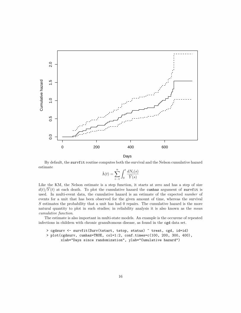
> vfit <- survfit(Surv(time1, time2, status) ~1, data=vdata, id=id)

> plot(vfit, cumhaz=TRUE, xlab="Days", ylab="Cumulative hazard")

15

0 200 400 600

0.0

0.5

1.0

1.5

2.0

Days

Cum

ulat

ive

haza

rd

By default, the survfit routine computes both the survival and the Nelson cumulative hazardestimate

Λ(t) =

n∑i−1

∫ t

0

dNi(s)

Y (s)

Like the KM, the Nelson estimate is a step function, it starts at zero and has a step of sized(t)/Y (t) at each death. To plot the cumulative hazard the cumhaz argument of survfit isused. In multi-event data, the cumulative hazard is an estimate of the expected number ofevents for a unit that has been observed for the given amount of time, whereas the survivalS estimates the probability that a unit has had 0 repairs. The cumulative hazard is the morenatural quantity to plot in such studies; in reliability analysis it is also known as the meancumulative function.

The estimate is also important in multi-state models. An example is the occurene of repeatedinfections in children with chronic granultomous disease, as found in the cgd data set.

> cgdsurv <- survfit(Surv(tstart, tstop, status) ~ treat, cgd, id=id)

> plot(cgdsurv, cumhaz=TRUE, col=1:2, conf.times=c(100, 200, 300, 400),

xlab="Days since randomization", ylab="Cumulative hazard")

16

0 100 200 300 400

0.0

0.5

1.0

1.5

2.0

Days since randomization

Cum

ulat

ive

haza

rd

2.3 Competing risks

The case of multiple event types, but only one event per subject is commonly known as competingrisks. We do not need the (time1, time2) data form for this case, since each subject has onlya single outcome, but we do need a way to identify different outcomes. In the prior sections,status was either a logical or 0/1 numeric variable that represents censoring (0 or FALSE) oran event (1 or TRUE), and the result of survfit was a single survival curve for each group. Forcompeting risks data status will be a factor; the first level of the factor is used to code censoringwhile the remaining ones are possible outcomes.

2.3.1 Simple example

Here is a simple competing risks example where the three endpoints are labeled as a, b and c.

> crdata <- data.frame(time= c(1:8, 6:8),

endpoint=factor(c(1,1,2,0,1,1,3,0,2,3,0),

labels=c("censor", "a", "b", "c")),

istate=rep("entry", 11),

id= LETTERS[1:11])

> tfit <- survfit(Surv(time, endpoint) ~ 1, data=crdata, id=id, istate=istate)

> dim(tfit)

17

strata states

1 4

> summary(tfit)

Call: survfit(formula = Surv(time, endpoint) ~ 1, data = crdata, id = id,

istate = istate)

time n.risk n.event P(entry) P(a) P(b) P(c)

1 11 1 0.909 0.0909 0.0000 0.000

2 10 1 0.818 0.1818 0.0000 0.000

3 9 1 0.727 0.1818 0.0909 0.000

5 7 1 0.623 0.2857 0.0909 0.000

6 6 2 0.416 0.3896 0.1948 0.000

7 4 2 0.208 0.3896 0.1948 0.208

The resulting object tfit contains an estimate of P (state), the probability of being in each stateat each time t. P is a matrix with one row for each time and one column for each of the fourstates a–c and “still in the starting state”. By definition each row of P sums to 1. We will alsouse the notation p(t) where p is a vector with one element per state and pj(t) is the fraction instate j at time t. The plot below shows all 4 curves. (Since they sum to 1 one of the 4 curves isredundant, often the entry state is omitted since it is the least interesting.) In the plot.survfitfunction there is the argument noplot="(s0)" which indicates that curves for state (s0) will notbe plotted. If we had not specified istate in the call to survfit, the default label for the initialstate would have been “s0” and t he solid curve would not have been plotted.

> plot(tfit, col=1:4, lty=1:4, lwd=2, ylab="Probability in state")

18

0 2 4 6 8

0.0

0.2

0.4

0.6

0.8

1.0

Pro

babi

lity

in s

tate

The resulting survfms object appears as a matrix and can be subscripted as such, with acolumn for each state and rows for each group, each unique combination of values on the righthand side of the formula is a group or strata. This makes it simple to display a subset of thecurves using plot or lines commands. The entry state in the above fit, for instance, can bedisplayed with plot(tfit[,1]).

> dim(tfit)

strata states

1 4

> tfit$states

[1] "entry" "a" "b" "c"

The curves are computed using the Aalen-Johansen estimator. This is an important concept,and so we work it out below.

1. The starting point is the column vector p(0) = (1, 0, 0, 0), everyone starts in the first state.2. At time 1, the first event time, form the 4 by 4 transition matrix T1

T (1) =

10/11 1/11 0/11 0/11

0 1 0 00 0 1 00 0 0 1

p(1) = p(0)T1

The first row of T (1) describes the disposition of everyone who is in state 1 and underobservation at time 1: 10/11 stay in state 1 and 1 subject transitions to state a. There is no

19

one in the other 3 states, so rows 2–4 are technically undefined; use a default “stay in the samestate” row which has 1 on the diagonal. (Since no one ever leaves states a, b, or c, the bottomthree rows of T will continue to have this form.)

3. At time 2 the first row will be (9/10, 0, 1/10, 0), and p(2) = p(1)T (2) = p(0)T (1)T (2).Continue this until the last event time. At a time point with only censoring, such as time 4,

T would be the identity matrix.It is straightforward to show that when there are only two states of alive -> dead, then p1(t)

replicates the Kaplan-Meier computation. For competing risks data such as the simple exampleabove, p(t) replicates the cumulative incidence (CI) estimator. That is, both the KM and CI areboth special cases of the Aalen-Johansen. The AJ is more general, however; a given subject canhave multiple transitions from state to state, including transitions to a state that was visitedearlier.

2.3.2 Monoclonal gammopathy

The mgus2 data set contains information of 1384 subjects who were who were found to have aparticular pattern on a laboratory test (monoclonal gammopathy of undetermined significanceor MGUS). The genesis of the study was a suspicion that such a result might indicate a predis-position to plasma cell malignancies such a multiple myeloma; subjects were followed forward toassess whether an excess did occur. The mean age at diagnosis is 63 years, so death from othercauses will be an important competing risk. Here are a few observations of the data set, one ofwhich experienced progression to a plasma cell malignancy.

> mgus2[55:59, -(4:7)]

id age sex ptime pstat futime death

55 55 82 F 94 0 94 1

56 56 78 M 29 1 44 1

57 57 79 F 84 0 84 1

58 58 72 F 321 0 321 1

59 59 80 F 147 0 147 1

To generate competing risk curves create a new (etime, event) pair. Since each subject hasat most 1 transition, we do not need a multi-line (time1, time2) dataset.

> event <- with(mgus2, ifelse(pstat==1, 1, 2*death))

> event <- factor(event, 0:2, c("censored", "progression", "death"))

> etime <- with(mgus2, ifelse(pstat==1, ptime, futime))

> crfit <- survfit(Surv(etime, event) ~ sex, mgus2)

> crfit

Call: survfit(formula = Surv(etime, event) ~ sex, data = mgus2)

n nevent rmean*

sex=F, (s0) 631 0 139.01247

sex=M, (s0) 753 0 122.97693

sex=F, progression 631 59 42.77078

sex=M, progression 753 56 31.82962

20

sex=F, death 631 370 242.21675

sex=M, death 753 490 269.19344

*mean time in state, restricted (max time = 424 )

> plot(crfit, col=1:2, noplot="",

lty=c(3,3,2,2,1,1), lwd=2, xscale=12,

xlab="Years post diagnosis", ylab="P(state)")

> legend(240, .65, c("Female, death", "Male, death", "malignancy", "(s0)"),

lty=c(1,1,2,3), col=c(1,2,1,1), bty='n', lwd=2)

0 5 10 15 20 25 30 35

0.0

0.2

0.4

0.6

0.8

1.0

Years post diagnosis

P(s

tate

) Female, deathMale, deathmalignancy(s0)

There are 3 curves for females, one for each of the three states, and 3 for males. The threecurves sum to 1 at any given time (everyone has to be somewhere), and the default action forplot.survfit is to leave out the “still in original state” curve (s0) since it is usually the leastinteresting, but in this case we have shown all 3. We will return to this example when exploringmodels.

A common mistake with competing risks is to use the Kaplan-Meier separately on each eventtype while treating other event types as censored. The next plot is an example of this for thePCM endpoint.

> pcmbad <- survfit(Surv(etime, pstat) ~ sex, data=mgus2)

> plot(pcmbad[2], mark.time=FALSE, lwd=2, fun="event", conf.int=FALSE, xscale=12,

xlab="Years post diagnosis", ylab="Fraction with PCM")

> lines(crfit[2,2], lty=2, lwd=2, mark.time=FALSE, conf.int=FALSE)

21

> legend(0, .25, c("Males, PCM, incorrect curve", "Males, PCM, competing risk"),

col=1, lwd=2, lty=c(1,2), bty='n')

0 5 10 15 20 25 30 35

0.00

0.05

0.10

0.15

0.20

0.25

Years post diagnosis

Fra

ctio

n w

ith P

CM

Males, PCM, incorrect curveMales, PCM, competing risk

There are two problems with the pcmbad fit. The first is that it attempts to estimate theexpected occurrence of plasma cell malignancy (PCM) if all other causes of death were to bedisallowed. In this hypothetical world it is indeed true that many more subjects would progressto PCM (the incorrect curve is higher), but it is also not a world that any of us will ever inhabit.This author views the result in much the same light as a discussion of survival after the zombieapocalypse. The second problem is that the computation for this hypothetical case is only correctif all of the competing endpoints are independent, a situation which is almost never true. Wethus have an unreliable estimate of an uninteresting quantity. The competing risks curve, onthe other hand, estimates the fraction of MGUS subjects who will experience PCM, a quantitysometimes known as the lifetime risk, and one which is actually observable.

The last example chose to plot only a subset of the curves, something that is often desirablein competing risks problems to avoid a “tangle of yarn” plot that simply has too many elements.This is done by subscripting the survfit object. For subscripting, multi-state curves behaveas a matrix with the outcomes as the second subscript. The columns are in order of the levelsof event, i.e., as displayed by our earlier call to table(event). The first subscript indexes thegroups formed by the right hand side of the model formula, and will be in the same order assimple survival curves. Thus mfit2[2,2] corresponds to males (2) and the PCM endpoint (2).Curves are listed and plotted in the usual matrix order of R.

> dim(crfit)

22

strata states

2 3

> crfit$strata

sex=F sex=M

227 227

> crfit$states

[1] "(s0)" "progression" "death"

One surprising aspect of multi-state data is that hazards can be estimated independentlyalthough probabilities cannot. If you look at the cumulative hazard estimate from the pcmbad

fit above using, for instance, plot(pcmbac, cumhaz=TRUE) you will find that it is identical tothe cumulative hazard estimate from the joint fit. This will arise again with Cox models.

2.3.3 Variance

The variance of the AJ estimate is computed using an infinitesimal jackknife (IJ) matrix, whichcontains the influence of each subject on the estimator; formally the derivative with respectto each subject’s case weight. For a single simple survival curve that has k unique values, forinstance, the IJ matrix will have n rows and k columns, one row per subject. Columns of thematrix sum to zero, by definition, and the variance at a time point t will be the column sums of(IJ)2. For a competing risk problem the crfit object above will contain a matrix pstate withk rows and one column for each state, where k is the number of unique time points; and the IJis an array of dimension (n, k, p). In the case of simple survival and all case weights =1, the IJvariance collapses to the well known Greenwood variance estimate.

2.4 Multi-state data

The most general multi-state data will have multiple outcomes and multiple endpoints per sub-ject. In this case, we will need to use the (time1, time2) form for each subject. The datasetstructure is similar to that for time varying covariates in a Cox model: the time variable will beintervals (t1, t2] which are open on the left and closed on the right, and a given subject will havemultiple lines of data. But instead of covariates changing from line to line, in this case the statusvariable changes; it contains the state that was entered at time t2. There are a few restrictions.

� An identifier variable is needed to indicate which rows of the dataframe belong to eachsubject. If the id argument is missing, the code assumes that each row of data is aseparate subject, which leads to a nonsense estimate when there are actually multiple rowsper subject.

� Subjects do not have to enter at time 0 or all at the same time, but each must traverse aconnected segment of time. Disjoint intervals such as the pair (0, 5], (8, 10] are illegal.

� A subject cannot change groups. Any covariates on the right hand side of the formulamust remain constant within subject. (This function is not a way to create supposed‘time-dependent’ survival curves.)

� Subjects may have case weights, and these weights may change over time for a subject.

23

The istate argument can be used to designate a subject’s state at the start of each t1, t2time interval. Like variables in the formula, it is searched for in the data argument. If it isnot present, every subject is assumed to start in a common entry state which is given the name“(s0)”. The parentheses are an echo of “(Intercept)” in a linear model and show a label that wasprovided by the program rather than the data. The distribution of states just prior to the firstevent time is treated as the initial distribution of states. In common with ordinary survival, anyobservation which is censored before the first event time has no impact on the results.

2.4.1 Myeloid data

The myeloid data set contains data from a clinical trial in subjects with acute myeloid leukemia.To protect patient confidentiality the data set in the survival package has been slightly perturbed,but results are essentially unchanged. In this comparison of two conditioning regimens, thecanonical path for a subject is initial therapy → complete response (CR) → hematologic stemcell transplant (SCT) → sustained remission, followed by relapse or death. Not everyone followsthis ideal path, of course.

> myeloid[1:5,]

id trt sex futime death txtime crtime rltime

1 1 B f 235 1 NA 44 113

2 2 A m 286 1 200 NA NA

3 3 A f 1983 0 NA 38 NA

4 4 B f 2137 0 245 25 NA

5 5 B f 326 1 112 56 200

The first few rows of data are shown above. The data set contains the follow-up time and statusat last follow-up for each subject, along with the time to transplant (txtime), complete response(crtime) or relapse after CR (rltime). Subject 1 did not receive a transplant, as shown by theNA value, and subject 2 did not achieve CR.

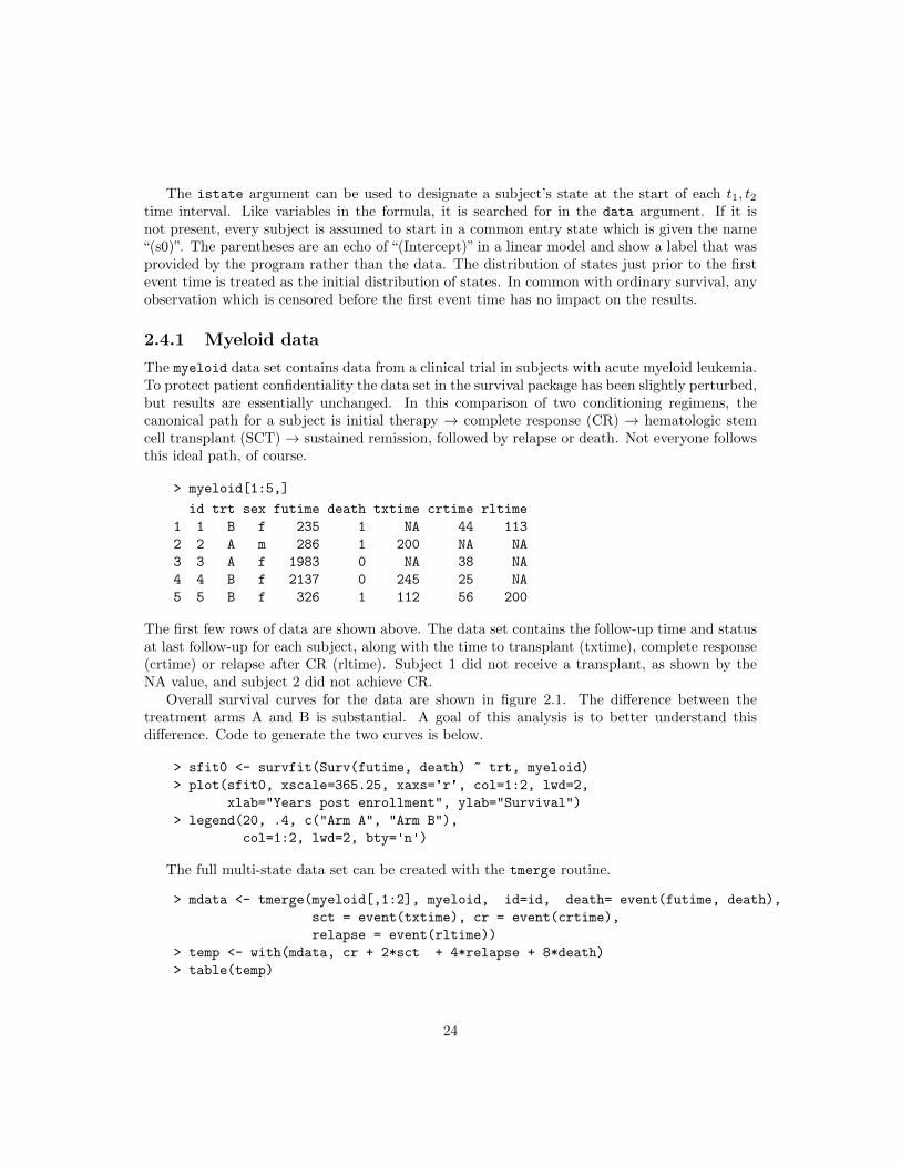
Overall survival curves for the data are shown in figure 2.1. The difference between thetreatment arms A and B is substantial. A goal of this analysis is to better understand thisdifference. Code to generate the two curves is below.

> sfit0 <- survfit(Surv(futime, death) ~ trt, myeloid)

> plot(sfit0, xscale=365.25, xaxs='r', col=1:2, lwd=2,

xlab="Years post enrollment", ylab="Survival")

> legend(20, .4, c("Arm A", "Arm B"),

col=1:2, lwd=2, bty='n')

The full multi-state data set can be created with the tmerge routine.

> mdata <- tmerge(myeloid[,1:2], myeloid, id=id, death= event(futime, death),

sct = event(txtime), cr = event(crtime),

relapse = event(rltime))

> temp <- with(mdata, cr + 2*sct + 4*relapse + 8*death)

> table(temp)

24

0 1 2 3 4 5 6

0.0

0.2

0.4

0.6

0.8

1.0

Years post enrollment

Sur

viva

l

Arm AArm B

Figure 2.1: Overall survival curves for the two treatments.

25

temp

0 1 2 3 4 8

325 453 363 1 226 320

Our check shows that there is one subject who had CR and stem cell transplant on the sameday (temp=3). To avoid length 0 intervals, we break the tie so that complete response (CR)happens first. (Students may be surprised to see anomalies like this, since they never appear intextbook data sets. In real data such issues always appear.)

> tdata <- myeloid # temporary working copy

> tied <- with(tdata, (!is.na(crtime) & !is.na(txtime) & crtime==txtime))

> tdata$crtime[tied] <- tdata$crtime[tied] -1

> mdata <- tmerge(tdata[,1:2], tdata, id=id, death= event(futime, death),

sct = event(txtime), cr = event(crtime),

relapse = event(rltime),

priorcr = tdc(crtime), priortx = tdc(txtime))

> temp <- with(mdata, cr + 2*sct + 4*relapse + 8*death)

> table(temp)

temp

0 1 2 4 8

325 454 364 226 320

> mdata$event <- factor(temp, c(0,1,2,4,8),

c("none", "CR", "SCT", "relapse", "death"))

> mdata[1:7, c("id", "trt", "tstart", "tstop", "event", "priorcr", "priortx")]

id trt tstart tstop event priorcr priortx

1 1 B 0 44 CR 0 0

2 1 B 44 113 relapse 1 0

3 1 B 113 235 death 1 0

4 2 A 0 200 SCT 0 0

5 2 A 200 286 death 0 1

6 3 A 0 38 CR 0 0

7 3 A 38 1983 none 1 0

Subject 1 has a CR on day 44, relapse on day 113, death on day 235 and did not receive astem cell transplant. The data for the first three subjects looks good. Check it out a little morethoroughly.

> survcheck(Surv(tstart, tstop, event) ~1, mdata, id=id)

Call:

survcheck(formula = Surv(tstart, tstop, event) ~ 1, data = mdata,

id = id)

646 subjects available for analysis

Transitions table:

to

from CR SCT relapse death (censored)

26

(s0) 443 106 13 55 29

CR 0 159 168 17 110

SCT 11 0 45 149 158

relapse 0 99 0 99 28

death 0 0 0 0 0

Number of subjects with 0, 1, ... transitions to each state:

count

state 0 1 2 3 4

CR 192 454 0 0 0

SCT 282 364 0 0 0

relapse 420 226 0 0 0

death 326 320 0 0 0

(any) 29 201 174 153 89

The second table shows that no single subject had more than one CR, SCT, relapse, or death;the intention of the study was to count only the first of each of these, so this is as expected.Several subjects visited all four intermediate states. The transitions table shows 11 subjectswho achieved CR after stem cell transplant and another 106 who received a transplant beforeachieving CR, both of which are deviations from the “ideal” pathway. No subjects went fromdeath to another state (which is good).

For investigating the data we would like to add a set of alternate endpoints.

1. The competing risk of CR and death, ignoring other states. This is used to estimate thefraction who ever achieved a complete response.

2. The competing risk of SCT and death, ignoring other states.

3. An endpoint that distinguishes death after SCT from death before SCT.

Each of these can be accomplished by adding further outcome variables to the data set, we willnot need to change the time intervals.

> levels(mdata$event)

[1] "none" "CR" "SCT" "relapse" "death"

> temp1 <- with(mdata, ifelse(priorcr, 0, c(0,1,0,0,2)[event]))

> mdata$crstat <- factor(temp1, 0:2, c("none", "CR", "death"))

> temp2 <- with(mdata, ifelse(priortx, 0, c(0,0,1,0,2)[event]))

> mdata$txstat <- factor(temp2, 0:2, c("censor", "SCT", "death"))

> temp3 <- with(mdata, c(0,0,1,0,2)[event] + priortx)

> mdata$tx2 <- factor(temp3, 0:3,

c("censor", "SCT", "death w/o SCT", "death after SCT"))

Notice the use of the priorcr variable in defining crstat. This outcome variable treatscomplete response as a terminal state, which in turn means that no further transitions areallowed after reaching CR.

This data set is the basis for our first set of curves, which are shown in figure 2.2. The plotoverlays three separate survfit calls: standard survival until death, complete response with

27

0.0

0.2

0.4

0.6

Months post enrollment

Fra

ctio

n w

ith th

e en

dpoi

nt

0 6 12 24 36 48

A CRB CR

A transplantB transplant

A deathB death

Entry

CR

Death

Entry

Tx

Death

Entry Death

Figure 2.2: Overall survival curves: time to death, to transplant (Tx), and to complete response(CR). Each shows the estimated fraction of subjects who have ever reached the given state. Thevertical line at 2 months is for reference. The curves were limited to the first 48 months to moreclearly show early events. The right hand panel shows the state-space model for each pair ofcurves.

28

death as a competing risk, and transplant with death as a competing risk. For each fit we haveshown one selected state: the fraction who have died, fraction ever in CR, and fraction everto receive transplant, respectively. Most of the CR events happen before 2 months (the greenvertical line) and nearly all the additional CRs conferred by treatment B occur between months2 and 8. Most transplants happen after 2 months, which is consistent with the clinical guide oftransplant after CR. The survival advantage for treatment B begins between 4 and 6 months,which argues that it could be at least partially a consequence of the additional CR events.

The code to draw figure 2.2 is below. It can be separated into 5 parts:

1. Fits for the 3 endpoints are simple and found in the first set of lines. The crstat andtxstat variables are factors, which causes multi-state curves to be generated.

2. The layout and par commands are used to create a multi-part plot with curves on the leftand state space diagrams on the right, and to reduce the amount of white space betweenthem.

3. Draw a subset of the curves via subscripting. A multi-state survfit object appears to theuser as a matrix of curves, with one row for each group (treatment) and one column foreach state. The CR state is the second column in sfit2, for instance. The CR fit wasdrawn first simply because it has the greatest y-axis range, then the other curves addedusing the lines command.

4. Decoration of the plots. This includes the line types, colors, legend, choice of x-axis labels,etc.

5. Add the state space diagrams. The functions for this are described elsewhere in the vi-gnette.

> # I want to have the plots in months, it is simpler to fix time

> # once rather than repeat xscale many times

> tdata$futime <- tdata$futime * 12 /365.25

> mdata$tstart <- mdata$tstart * 12 /365.25

> mdata$tstop <- mdata$tstop * 12 /365.25

> sfit1 <- survfit(Surv(futime, death) ~ trt, tdata) # survival

> sfit2 <- survfit(Surv(tstart, tstop, crstat) ~ trt,

data= mdata, id = id) # CR

> sfit3 <- survfit(Surv(tstart, tstop, txstat) ~ trt,

data= mdata, id =id) # SCT

> layout(matrix(c(1,1,1,2,3,4), 3,2), widths=2:1)

> oldpar <- par(mar=c(5.1, 4.1, 1.1, .1))

> mlim <- c(0, 48) # and only show the first 4 years

> plot(sfit2[,"CR"], xlim=mlim,

lty=3, lwd=2, col=1:2, xaxt='n',

xlab="Months post enrollment", ylab="Fraction with the endpoint")

> lines(sfit1, mark.time=FALSE, xlim=mlim,

fun='event', col=1:2, lwd=2)

> lines(sfit3[,"SCT"], xlim=mlim, col=1:2,

29

lty=2, lwd=2)

> xtime <- c(0, 6, 12, 24, 36, 48)

> axis(1, xtime, xtime) #axis marks every year rather than 10 months

> temp <- outer(c("A", "B"), c("CR", "transplant", "death"), paste)

> temp[7] <- ""

> legend(25, .3, temp[c(1,2,7,3,4,7,5,6,7)], lty=c(3,3,3, 2,2,2 ,1,1,1),

col=c(1,2,0), bty='n', lwd=2)

> abline(v=2, lty=2, col=3)

> # add the state space diagrams

> par(mar=c(4,.1,1,1))

> crisk(c("Entry", "CR", "Death"), alty=3)

> crisk(c("Entry", "Tx", "Death"), alty=2)

> crisk(c("Entry","Death"))

> par(oldpar)

> layout(1)

The association between a particular curve and its corresponding state space diagram iscritical. As we will see below, many different models are possible and it is easy to get confused.Attachment of a diagram directly to each curve, as was done above, will not necessarily be day-to-day practice, but the state space should always be foremost. If nothing else, draw it on ascrap of paper and tape it to the side of the terminal when creating a data set and plots.

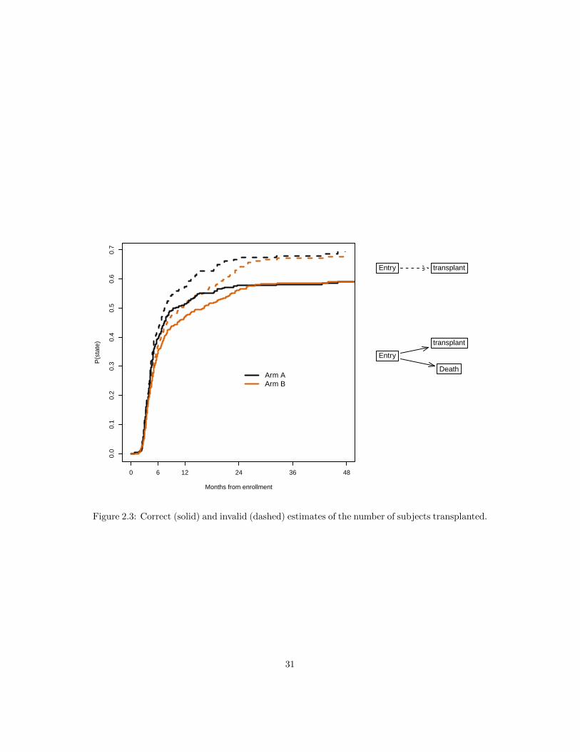
Figure 2.3 shows the transplant curves overlaid with the naive KM that censors subjects atdeath. There is no difference in the initial portion as no deaths have yet intervened, but the finalportion overstates the transplant outcome by more than 10%.

1. The key problem with the naive estimate is that subjects who die can never have a trans-plant. The result of censoring them is an estimate of the “fraction who would be trans-planted, if death before transplant were abolished”. This is not a real world quantity.

2. In order to estimate this fictional quantity one needs to assume that death is uninforma-tive with respect to future disease progression. The early deaths in months 0–2, beforetransplant begins, are however a very different class of patient. Non-informative censoringis untenable.

We are left with an unreliable estimate of an uninteresting quantity. Mislabeling any true stateas censoring is always a mistake, one that will not be repeated here. Here is the code for figure2.3. The use of a logical (true/false) as the status variable in the Surv call leads to ordinarysurvival calculations.

> badfit <- survfit(Surv(tstart, tstop, event=="SCT") ~ trt,

id=id, mdata, subset=(priortx==0))

> layout(matrix(c(1,1,1,2,3,4), 3,2), widths=2:1)

> oldpar <- par(mar=c(5.1, 4.1, 1.1, .1))

> plot(badfit, fun="event", xmax=48, xaxt='n', col=1:2, lty=2, lwd=2,

xlab="Months from enrollment", ylab="P(state)")

> axis(1, xtime, xtime)

> lines(sfit3[,2], xmax=48, col=1:2, lwd=2)

> legend(24, .3, c("Arm A", "Arm B"), lty=1, lwd=2,

30

0.0

0.1

0.2

0.3

0.4

0.5

0.6

0.7

Months from enrollment

P(s

tate

)

0 6 12 24 36 48

Arm AArm B

Entry transplant

Entry

transplant

Death

Figure 2.3: Correct (solid) and invalid (dashed) estimates of the number of subjects transplanted.

31

0 2 4 6 8 10 12

0.0

0.2

0.4

0.6

Months

CR

Entry

CR

Death

Entry

CR

Death/Relapse

Figure 2.4: Models for ‘ever in CR’ and ‘currently in CR’; the only difference is an additionaltransition. Both models ignore transplant.

col=1:2, bty='n', cex=1.2)

> par(mar=c(4,.1,1,1))

> crisk(c("Entry", "transplant"), alty=2, cex=1.2)

> crisk(c("Entry","transplant", "Death"), cex=1.2)

> par(oldpar)

> layout(1)

Complete response is a goal of the initial therapy; figure 2.4 looks more closely at this. Aswas noted before arm B has an increased number of late responses. The duration of response isalso increased: the solid curves show the number of subjects still in response, and we see thatthey spread farther apart than the dotted “ever in response” curves. The figure shows only thefirst eight months in order to better visualize the details, but continuing the curves out to 48months reveals a similar pattern. Here is the code to create the figure.

> cr2 <- mdata$event

> cr2[cr2=="SCT"] <- "none" # ignore transplants

> crsurv <- survfit(Surv(tstart, tstop, cr2) ~ trt,

data= mdata, id=id, influence=TRUE)

> layout(matrix(c(1,1,2,3), 2,2), widths=2:1)

32

> oldpar <- par(mar=c(5.1, 4.1, 1.1, .1))

> plot(sfit2[,2], lty=3, lwd=2, col=1:2, xmax=12,

xlab="Months", ylab="CR")

> lines(crsurv[,2], lty=1, lwd=2, col=1:2)

> par(mar=c(4, .1, 1, 1))

> crisk( c("Entry","CR", "Death"), alty=3)

> state3(c("Entry", "CR", "Death/Relapse"))

> par(oldpar)

> layout(1)

The above code created yet another event variable so as to ignore transitions to the transplantstate. They become a non-event, in the same way that extra lines with a status of zero are usedto create time-dependent covariates for a Cox model fit.

The survfit call above included the influence=TRUE argument, which causes the influencearray to be calculated and returned. It contains, for each subject, that subject’s influence on thetime by state matrix of results and allows for calculation of the standard error of the restrictedmean. We will return to this in a later section.

> print(crsurv, rmean=48, digits=2)

Call: survfit(formula = Surv(tstart, tstop, cr2) ~ trt, data = mdata,

id = id, influence = TRUE)

n nevent rmean std(rmean)*

trt=A, (s0) 693 0 7.1 0.78

trt=B, (s0) 739 0 5.6 0.65

trt=A, CR 693 206 16.3 1.13

trt=B, CR 739 248 21.2 1.12

trt=A, SCT 693 0 0.0 0.00

trt=B, SCT 739 0 0.0 0.00

trt=A, relapse 693 109 4.3 0.56

trt=B, relapse 739 117 5.5 0.61

trt=A, death 693 171 20.2 1.10

trt=B, death 739 149 15.6 1.01

*mean time in state, restricted (max time = 48 )

The restricted mean time in the CR state is extended by 21.2 - 16.3 = 4.89 months. Aquestion which immediately gets asked is whether this difference is “significant”, to which thereare two answers. The first and more important is to ask whether 5 months is an importantgain from either a clinical or patient perspective. The overall restricted mean survival for thestudy is approximately 30 of the first 48 months post entry (use print(sfit1, rmean=48)); onthis backdrop an extra 5 months in CR might or might not be an meaningful advantage froma patient’s point of view. The less important answer is to test whether the apparent gain issufficiently rare from a mathematical point of view, i.e., “statistical” significance. The standarderrors of the two values are 1.1 and 1.1, and since they are based on disjoint subjects the valuesare independent, leading to a standard error for the difference of

√1.12 + 1.12 = 1.6. The 5

month difference is more than 3 standard errors, so highly significant.In summary

33

0.0

0.1

0.2

0.3

0.4

Months

Tran

spla

nted

0 6 12 24 36 48

A, transplant without CRB, transplant without CRA, transplant after CRB, transplant after CR

Entry

CRTransplant

Transplant

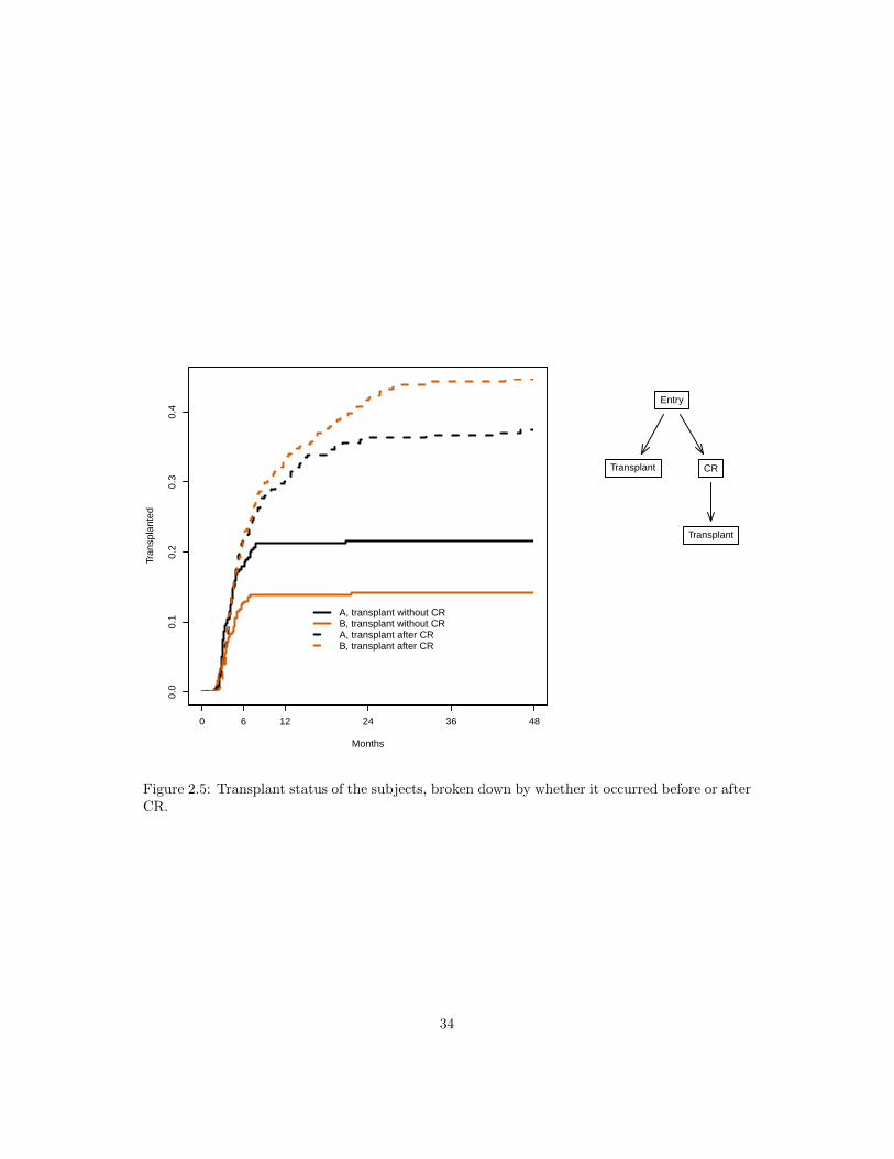
Figure 2.5: Transplant status of the subjects, broken down by whether it occurred before or afterCR.

34

� Arm B adds late complete responses (about 4%); there are 206/317 in arm B vs. 248/329in arm B.

� The difference in 4 year survival is about 6%.

� There is approximately 2 months longer average duration of CR (of 48).

CR → transplant is the target treatment path for a patient; given the improvements listedabove why does figure 2.2 show no change in the number transplanted? Figure 2.5 shows thetransplants broken down by whether this happened before or after complete response. Mostof the non-CR transplants happen by 10 months. One possible explanation is that once it isapparent to the patient/physician pair that CR is not going to occur, they proceed forward withother treatment options. The extra CR events on arm B, which occur between 2 and 8 months,lead to a consequent increase in transplant as well, but at a later time of 12–24 months: for asubject in CR we can perhaps afford to defer the transplant date.

Computation is again based on a manipulation of the event variable: in this case dividing thetransplant state into two sub-states based on the presence of a prior CR. The code makes useof the time-dependent covariate priorcr. (Because of scheduling constraints within a hospitalit is unlikely that a CR that is within a few days prior to transplant could have effected thedecision to schedule a transplant, however. An alternate breakdown that might be useful wouldbe “transplant without CR or within 7 days after CR” versus those that are more than a weeklater. There are many sensible questions that can be asked.)

> event2 <- with(mdata, ifelse(event=="SCT" & priorcr==1, 6,

as.numeric(event)))

> event2 <- factor(event2, 1:6, c(levels(mdata$event), "SCT after CR"))

> txsurv <- survfit(Surv(tstart, tstop, event2) ~ trt, mdata, id=id,

subset=(priortx ==0))

> dim(txsurv) # number of strata by number of states

strata states

2 6

> txsurv$states # Names of states

[1] "(s0)" "CR" "SCT" "relapse"

[5] "death" "SCT after CR"

> layout(matrix(c(1,1,1,2,2,0),3,2), widths=2:1)

> oldpar <- par(mar=c(5.1, 4.1, 1,.1))

> plot(txsurv[,c(3,6)], col=1:2, lty=c(1,1,2,2), lwd=2, xmax=48,

xaxt='n', xlab="Months", ylab="Transplanted")

> axis(1, xtime, xtime)

> legend(15, .13, c("A, transplant without CR", "B, transplant without CR",

"A, transplant after CR", "B, transplant after CR"),

col=1:2, lty=c(1,1,2,2), lwd=2, bty='n')

> state4() # add the state figure

> par(oldpar)

Figure 2.6 shows the full set of state occupancy probabilities for the cohort over the first 4years. At each point in time the curves estimate the fraction of subjects currently in that state.

35

0.0

0.1

0.2

0.3

0.4

0.5

0.6

0.7

Months

Cur

rent

sta

te

0 6 12 24 36 48

Death

CR

Transplant

Recurrence

Entry

CR Tx Rel

Death

Figure 2.6: The full multi-state curves for the two treatment arms.

36

The total who are in the transplant state peaks at about 9 months and then decreases as subjectsrelapse or die; the curve rises whenever someone receives a transplant and goes down wheneversomeone leaves the state. At 36 months treatment arm B (dashed) has a lower fraction whohave died, the survivors are about evenly split between those who have received a transplant andthose whose last state is a complete response (only a few of the latter are post transplant). Thefraction currently in relapse – a transient state – is about 5% for each arm. The figure omitsthe curve for “still in the entry state”. The reason is that at any point in time the sum of the 5possible states is 1 — everyone has to be somewhere. Thus one of the curves is redundant, andthe fraction still in the entry state is the least interesting of them.

> sfit4 <- survfit(Surv(tstart, tstop, event) ~ trt, mdata, id=id)

> sfit4$transitions

to

from CR SCT relapse death (censored)

(s0) 443 106 13 55 29

CR 0 159 168 17 110

SCT 11 0 45 149 158

relapse 0 99 0 99 28

death 0 0 0 0 0

> layout(matrix(1:2,1,2), widths=2:1)

> oldpar <- par(mar=c(5.1, 4.1, 1,.1))

> plot(sfit4, col=rep(1:4,each=2), lwd=2, lty=1:2, xmax=48, xaxt='n',

xlab="Months", ylab="Current state")

> axis(1, xtime, xtime)

> text(c(40, 40, 40, 40), c(.51, .13, .32, .01),

c("Death", "CR", "Transplant", "Recurrence"), col=c(4,1,2,3))

> par(mar=c(5.1, .1, 1, .1))

> state5()

> par(oldpar)

The transitions table above shows 55 direct transitions from entry to death, i.e., subjects whodie without experiencing any of the other intermediate points, 159 who go from CR to transplant(as expected), 11 who go from transplant to CR, etc. No one was observed to go from relapse toCR in the data set, this serves as a data check since it should not be possible per the data entryplan.

2.5 Influence matrix

For one of the curves above we returned the influence array. For each value in the matrix P =probability in state and each subject i in the data set, this contains the effect of that subject oneach value in P . Formally,

Dij(t) =∂pj(t)

∂wi

∣∣∣∣w

where Dij(t) is the influence of subject i on pj(t), and pj(t) is the estimated probability for statej at time t. This is known as the infinitesimal jackknife (among other labels).

37

> crsurv <- survfit(Surv(tstart, tstop, cr2) ~ trt,

data= mdata, id=id, influence=TRUE)

> curveA <- crsurv[1,] # select treatment A

> dim(curveA) # P matrix for treatement A

strata states

1 5

> curveA$states

[1] "(s0)" "CR" "SCT" "relapse" "death"

> dim(curveA$pstate) # 426 time points, 5 states

[1] 426 5

> dim(curveA$influence) # influence matrix for treatment A

[1] 317 426 5

> table(myeloid$trt)

A B

317 329

For treatment arm A there are 317 subjects and 426 time points in the P matrix. Theinfluence array has subject as the first dimension, and for each subject it has an image of theP matrix containing that subject’s influence on each value in P , i.e., influence[1, ,] is theinfluence of subject 1 on P . For this data set everyone starts in the entry state, so p(0) = thefirst row of pstate will be (1, 0, 0, 0, 0) and the influence of each subject on this row is 0; thisdoes not hold if not all subjects start in the same state.

As an exercise we will calculate the mean time in state out to 48 weeks. This is the areaunder the individual curves from time 0 to 48. Since the curves are step functions this is simplesum of rectangles, treating any intervals after 48 months as having 0 width.

> t48 <- pmin(48, curveA$time)

> delta <- diff(c(t48, 48)) # width of intervals

> rfun <- function(pmat, delta) colSums(pmat * delta) #area under the curve

> rmean <- rfun(curveA$pstate, delta)

> # Apply the same calculation to each subject's influence slice

> inf <- apply(curveA$influence, 1, rfun, delta=delta)

> # inf is now a 5 state by 310 subject matrix, containing the IJ estimates

> # on the AUC or mean time. The sum of squares is a variance.

> se.rmean <- sqrt(rowSums(inf^2))

> round(rbind(rmean, se.rmean), 2)

[,1] [,2] [,3] [,4] [,5]

rmean 7.10 16.34 0 4.31 20.24

se.rmean 0.78 1.13 0 0.56 1.10

> print(curveA, rmean=48, digits=2)

Call: survfit(formula = Surv(tstart, tstop, cr2) ~ trt, data = mdata,

id = id, influence = TRUE)

n nevent rmean std(rmean)*

(s0) 693 0 7.1 0.78

38

CR 693 206 16.3 1.13

SCT 693 0 0.0 0.00

relapse 693 109 4.3 0.56

death 693 171 20.2 1.10

*mean time in state, restricted (max time = 48 )

The last lines verify that this is exactly the calculation done by the print.survfitms func-tion; the results can also be found in the table component returned by summary.survfitms.

In general, let Ui be the influence of subject i. For some function f(P ) of the probabilityin state matrix pstate, the influence of subject i will be δi = f(P + Ui) − f(P ) and theinfinitesimal jackknife estimate of variance will be

∑i δ

2. For the simple case of adding uprectangles f(P +Ui)−f(P ) = f(Ui) leading to particularly simple code, but this will not alwaysbe the case.

2.6 Differences in survival

There is a single function survdiff to test for differences between 2 or more survival curves.It implements the Gρ family of Fleming and Harrington [?]. A single parameter ρ controls theweights given to different survival times, ρ = 0 yields the log-rank test and ρ = 1 the Peto-Wilcoxon. Other values give a test that is intermediate to these two. The default value is ρ = 0.The log-rank test is equivalent to the score test from a Cox model with the group as a factorvariable.

The interpretation of the formula is the same as for survfit, i.e., variables on the right handside of the equation jointly break the patients into groups.

> survdiff(Surv(time, status) ~ x, aml)

Call:

survdiff(formula = Surv(time, status) ~ x, data = aml)

N Observed Expected (O-E)^2/E (O-E)^2/V

x=Maintained 11 7 10.69 1.27 3.4

x=Nonmaintained 12 11 7.31 1.86 3.4

Chisq= 3.4 on 1 degrees of freedom, p= 0.07

2.7 State space figures

The state space figures in the above example were drawn with a simple utility function statefig.It has two primary arguments along with standard graphical options of color, line type, etc.

1. A layout vector or matrix. A vector with values of (1, 3, 1) for instance will allocate onestate, then a column with 3 states, then one more state, proceeding from left to right. Amatrix with a single row will do the same, whereas a matrix with one column will proceedfrom top to bottom.

39

2. A k by k connection matrix C where k is the number of states. If Cij 6= 0 then an arrowis drawn from state i to state j. The row or column names of the matrix are used to labelthe states. The lines connecting the states can be straight or curved, see the help file foran example.

The first few state space diagrams were competing risk models, which use the following helperfunction. It accepts a vector of state names, where the first name is the starting state and theremainder are the possible outcomes.

> crisk <- function(what, horizontal = TRUE, ...) {

nstate <- length(what)

connect <- matrix(0, nstate, nstate,

dimnames=list(what, what))

connect[1,-1] <- 1 # an arrow from state 1 to each of the others

if (horizontal) statefig(c(1, nstate-1), connect, ...)

else statefig(matrix(c(1, nstate-1), ncol=1), connect, ...)

}

This next function draws a variation of the illness-death model. It has an initial state, anabsorbing state (normally death), and an optional intermediate state.

> state3 <- function(what, horizontal=TRUE, ...) {

if (length(what) != 3) stop("Should be 3 states")

connect <- matrix(c(0,0,0, 1,0,0, 1,1,0), 3,3,

dimnames=list(what, what))

if (horizontal) statefig(1:2, connect, ...)

else statefig(matrix(1:2, ncol=1), connect, ...)

}

The most complex of the state space figures has all 5 states.

> state5 <- function(what, ...) {

sname <- c("Entry", "CR", "Tx", "Rel", "Death")

connect <- matrix(0, 5, 5, dimnames=list(sname, sname))

connect[1, -1] <- c(1,1,1, 1.4)

connect[2, 3:5] <- c(1, 1.4, 1)

connect[3, c(2,4,5)] <- 1

connect[4, c(3,5)] <- 1

statefig(matrix(c(1,3,1)), connect, cex=.8, ...)

}

For figure 2.5 I want a third row with a single state, but don’t want that state centered. Forthis I need to create my own (x,y) coordinate list as the layout parameter. Coordinates must bebetween 0 and 1.

> state4 <- function() {

sname <- c("Entry", "CR", "Transplant", "Transplant")

layout <- cbind(x =c(1/2, 3/4, 1/4, 3/4),

y =c(5/6, 1/2, 1/2, 1/6))

40

connect <- matrix(0,4,4, dimnames=list(sname, sname))

connect[1, 2:3] <- 1

connect[2,4] <- 1

statefig(layout, connect)

}

The statefig function was written to do“good enough”state space figures quickly and easily, inthe hope that users will find it simple enough that diagrams are drawn early and often. Packagesdesigned for directed acyclic graphs (DAG) such as diagram, DiagrammeR, or dagR are far moreflexible and can create more nuanced and well decorated results.

2.7.1 Further notes

The Aalen-Johansen method used by survfit does not account for interval censoring, alsoknown as panel data, where a subject’s current state is recorded at some fixed time such asa medical center visit but the actual times of transitions are unknown. Such data requiresfurther assumptions about the transition process in order to model the outcomes and has a morecomplex likelihood. The msm package, for instance, deals with data of this type. If subjectsreliably come in at regular intervals then the difference between the two results can be small,e.g., the msm routine estimates time until progression occurred whereas survfit estimates timeuntil progression was observed.

� When using multi-state data to create Aalen-Johansen estimates, individuals are not al-lowed to have gaps in the middle of their time line. An example of this would be a dataset with (0, 30, pcm] and (50,70, death] as the two observations for a subject where thetime from 30-70 is not accounted for.

� Subjects must stay in the same group over their entire observation time, i.e., variables onthe right hand side of the equation cannot be time-dependent.

� A transition to the same state is allowed, e.g., observations of (0,50, 1], (50, 75, 3], (75, 89,4], (89, 93, 4] and (93, 100, 4] for a subject who goes from entry to state 1, then to state 3,and finally to state 4. However, a warning message is issued for the data set in this case,since stuttering may instead be the result of a coding mistake. The same result is obtainedif the last three observations were collapsed to a single row of (75, 100, 4].

41

Chapter 3

Cox model

The most commonly used models for survival data are those that model the transition ratefrom state to state, i.e., the arrows of figure 1.1. They are Poisson regression (3.1), the Cox orproportional hazards model (3.2) and the Aalen additive regression model (3.3), of which theCox model is far and away the most popular. As seen in the equations they are closely related.

λ(t) = ebeta0+β1x1+β2x2+... (3.1)

λ(t) = eβ0(t)+β1x1+β2x2+...

= λ0(t)eβ1x1+β2x2+... (3.2)

λ(t) = β0(t) + β1(t)x1 + β2(t)x2 + . . . (3.3)

(Textbooks on survival use λ(t), α(t) and h(t) in about equal proportions. There is no goodargument for any one versus another, but this author started his career with books that used λso that is what you will get.)

3.1 One event type, one event per subject

Single event data is the most common use for Cox models. We will use a data set that containsthe survival of 228 patients with advanced lung cancer.

> options(show.signif.stars=FALSE) # display statistical intelligence

> cfit1 <- coxph(Surv(time, status) ~ age + sex + wt.loss, data=lung)

> print(cfit1, digits=3)

Call:

coxph(formula = Surv(time, status) ~ age + sex + wt.loss, data = lung)

coef exp(coef) se(coef) z p

age 0.02009 1.02029 0.00966 2.08 0.0377

sex -0.52103 0.59391 0.17435 -2.99 0.0028

wt.loss 0.00076 1.00076 0.00619 0.12 0.9024

42

Likelihood ratio test=14.7 on 3 df, p=0.00212

n= 214, number of events= 152

(14 observations deleted due to missingness)

> summary(cfit1, digits=3)

Call:

coxph(formula = Surv(time, status) ~ age + sex + wt.loss, data = lung)

n= 214, number of events= 152

(14 observations deleted due to missingness)

coef exp(coef) se(coef) z Pr(>|z|)

age 0.0200882 1.0202913 0.0096644 2.079 0.0377

sex -0.5210319 0.5939074 0.1743541 -2.988 0.0028

wt.loss 0.0007596 1.0007599 0.0061934 0.123 0.9024

exp(coef) exp(-coef) lower .95 upper .95

age 1.0203 0.9801 1.0011 1.0398

sex 0.5939 1.6838 0.4220 0.8359

wt.loss 1.0008 0.9992 0.9887 1.0130

Concordance= 0.612 (se = 0.027 )

Likelihood ratio test= 14.67 on 3 df, p=0.002

Wald test = 13.98 on 3 df, p=0.003

Score (logrank) test = 14.24 on 3 df, p=0.003

> anova(cfit1)

Analysis of Deviance Table

Cox model: response is Surv(time, status)

Terms added sequentially (first to last)

loglik Chisq Df Pr(>|Chi|)

NULL -680.39

age -677.78 5.2273 1 0.022235

sex -673.06 9.4268 1 0.002138

wt.loss -673.06 0.0150 1 0.902592

As is usual with R modeling functions, the default print routine gives a short summary andthe summary routine a longer one. The anova command shows tests for each term in a model,added sequentially. We purposely avoid the innane addition of “significant stars” to any printout.Age and gender are strong predictors of survival, but the amount of recent weight loss was notinfluential.

The following functions can be used to extract portions of a coxph object.

� coef or coefficients: the vector of coefficients

� concordance: the concordance statistic for the model fit

43

� fitted: the fitted values, also known as linear predictors

� logLik: the partial likelihood

� model.frame: the model.frame of the data used in the fit

� model.matrix: the X matrix used in the fit

� nobs: the number of observations

� predict: a vector or matrix of predicted values

� residuals: a vector of residuals

� vcov: the variance-covariance matrix

� weights: the vector of case weights used in the fit

Further details about the contents of a coxph object can be found by help(’coxph.object’).The global na.action function has an important effect on the returned vector of residuals, as

shown below. This can be set per fit, but is more often set globally via the options() function.

> cfit1a <- coxph(Surv(time, status) ~ age + sex + wt.loss, data=lung,

na.action = na.omit)

> cfit1b <- coxph(Surv(time, status) ~ age + sex + wt.loss, data=lung,

na.action = na.exclude)

> r1 <- residuals(cfit1a)

> r2 <- residuals(cfit1b)

> length(r1)

[1] 214

> length(r2)

[1] 228

The fits have excluded 14 subjects with missing values for one or more covariates. The residualvector r1 omits those subjects from the residuals, while r2 returns a vector of the same lengthas the original data, containing NA for the omitted subjects. Which is preferred depends onwhat you want to do with the residuals. For instance mean(r1) is simpler using the first whileplot(lung$ph.ecog, r2) is simpler with the second.

Stratified Cox models are obtained by adding one or more strata terms to the model formula.In a stratified model each subject is compared only to subjects within their own stratum forcomputing the partial likelihood, and then the final results are summed over the strata. A usefulrule of thumb is that a variable included as a stratum is adjusted for in the most general way,at the price of not having an estimate of its effect. One common use of strata is to adjust forthe enrolling institution in a multi-center study, as below. We see that in this case the effect ofstratification is slight.

> cfit2 <- coxph(Surv(time, status) ~ age + sex + wt.loss + strata(inst),

data=lung)

> round(cbind(simple= coef(cfit1), stratified=coef(cfit2)), 4)

44

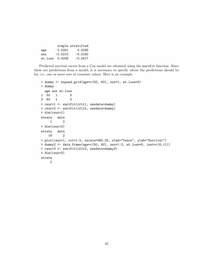
simple stratified

age 0.0201 0.0235

sex -0.5210 -0.5160

wt.loss 0.0008 -0.0017

Predicted survival curves from a Cox model are obtained using the survfit function. Sincethese are predictions from a model, it is necessary to specify whom the predictions should befor, i.e., one or more sets of covariate values. Here is an example.

> dummy <- expand.grid(age=c(50, 60), sex=1, wt.loss=5)

> dummy

age sex wt.loss

1 50 1 5

2 60 1 5

> csurv1 <- survfit(cfit1, newdata=dummy)

> csurv2 <- survfit(cfit2, newdata=dummy)

> dim(csurv1)

strata data

1 2

> dim(csurv2)

strata data

18 2

> plot(csurv1, col=1:2, xscale=365.25, xlab="Years", ylab="Survival")

> dummy2 <- data.frame(age=c(50, 60), sex=1:2, wt.loss=5, inst=c(6,11))

> csurv3 <- survfit(cfit2, newdata=dummy2)

> dim(csurv3)

strata

2

45

0.0 0.5 1.0 1.5 2.0 2.5

0.0

0.2

0.4

0.6

0.8

1.0

Years

Sur

viva

l

The simplifying aspects of the Cox model that make is so useful are exactly those that shouldbe verified, namely proportional hazards, additivity, linearity, and lack of any high leveragepoints. The first can be checked with the cox.zph function.

> zp1 <- cox.zph(cfit1)

> zp1

chisq df p

age 0.5077 1 0.48

sex 2.5489 1 0.11

wt.loss 0.0144 1 0.90

GLOBAL 3.0051 3 0.39

> plot(zp1[2], resid=FALSE)

> abline(coef(fit1)[2] ,0, lty=3)

46

Time

Bet

a(t)

for

sex

56 150 200 280 350 450 570 730

−2.

0−

1.5

−1.

0−

0.5

0.0

0.5

1.0

1.5

None of the test statistics for PH are remarkable. A simple check for linearity of age is toreplace the term with a smoothing spline.

> cfit3 <- coxph(Surv(time, status) ~ pspline(age) + sex + wt.loss, lung)

> print(cfit3, digits=2)

Call:

coxph(formula = Surv(time, status) ~ pspline(age) + sex + wt.loss,

data = lung)

coef se(coef) se2 Chisq DF p

pspline(age), linear 0.02011 0.00931 0.00931 4.66393 1.0 0.031

pspline(age), nonlin 3.02601 3.1 0.402

sex -0.53145 0.17549 0.17513 9.17105 1.0 0.002

wt.loss 0.00056 0.00619 0.00618 0.00818 1.0 0.928

Iterations: 4 outer, 12 Newton-Raphson

Theta= 0.8

Degrees of freedom for terms= 4.1 1.0 1.0

Likelihood ratio test=18 on 6.1 df, p=0.006

n= 214, number of events= 152

(14 observations deleted due to missingness)

> termplot(cfit3, term=1, se=TRUE)

> cfit4 <- update(cfit1, . ~ . + age*sex)

47

> anova(cfit1, cfit4)

Analysis of Deviance Table

Cox model: response is Surv(time, status)

Model 1: ~ age + sex + wt.loss

Model 2: ~ age + sex + wt.loss + age:sex

loglik Chisq Df P(>|Chi|)

1 -673.06

2 -672.88 0.3473 1 0.5557

40 50 60 70 80

−2

−1

01

2

age

Par

tial f

or p

splin

e(ag

e)

The age effect appears reasonbly linear. Additivity can be examined by adding and age bysex interaction, and again is not remarkable.

3.2 Repeating Events

Children with chronic granulotomous disease (CGD) are subject to repeated infections due to acompromised immune system. The cgd0 data set contains results of a clinical trial of gammainterferon as a treatment, the data set cdg contains the data reformatted into a (tstart, tstop,status) form: each child can have multiple rows which describe an interval of time, and status=1if that interval ends with an infection and 0 otherwise. A model with a single baseline hazard,known as the Andersen-Gill model, can be fit very simply. The study recruited subjects fromfour types of institutions, and there is an a priori belief that the four classes might recruit a

48

different type of subject. Adding the hospital category as a strata allows each group to have adifferent shape of baseline hazard.

> cfit1 <- coxph(Surv(tstart, tstop, status) ~ treat + inherit + steroids +

age + strata(hos.cat), data=cgd)

> print(cfit1, digits=2)

Call:

coxph(formula = Surv(tstart, tstop, status) ~ treat + inherit +

steroids + age + strata(hos.cat), data = cgd)

coef exp(coef) se(coef) z p

treatrIFN-g -1.113 0.328 0.267 -4.2 3e-05

inheritautosomal 0.430 1.537 0.250 1.7 0.09

steroids 1.258 3.517 0.573 2.2 0.03

age -0.036 0.964 0.015 -2.4 0.02

Likelihood ratio test=31 on 4 df, p=3.8e-06

n= 203, number of events= 76

Further examination shows that the fit is problematic in that only 3 of 128 children have steroids==1, so we refit without that variable.

> cfit2 <- coxph(Surv(tstart, tstop, status) ~ treat + inherit+

age + strata(hos.cat), data=cgd)

> print(cfit2, digits=2)

Call:

coxph(formula = Surv(tstart, tstop, status) ~ treat + inherit +

age + strata(hos.cat), data = cgd)

coef exp(coef) se(coef) z p

treatrIFN-g -1.089 0.337 0.265 -4.1 4e-05

inheritautosomal 0.406 1.500 0.249 1.6 0.10

age -0.033 0.967 0.015 -2.3 0.02

Likelihood ratio test=27 on 3 df, p=6.6e-06

n= 203, number of events= 76

Predicted survival and/or cumulative hazard curves can then be obtained from the fittedmodel. Prediction requires the user to specifiy who to predict; in this case we will use 4 hypo-thetical subjects on control/interferon treatment, at ages 7 and 20 (near the quantiles). Thiscreates a data frame with 4 rows.

> dummy <- expand.grid(age=c(6,12), inherit='X-linked',

treat=levels(cgd$treat))

> dummy

age inherit treat

1 6 X-linked placebo

49

2 12 X-linked placebo

3 6 X-linked rIFN-g

4 12 X-linked rIFN-g

> csurv <- survfit(cfit2, newdata=dummy)

> dim(csurv)

strata data

4 4

> plot(csurv[1,], fun="event", col=1:2, lty=c(1,1,2,2),

xlab="Days on study", ylab="Pr( any infection )")

0 100 200 300 400

0.0

0.2

0.4

0.6

0.8

Days on study

Pr(

any

infe

ctio

n )

The resulting object was subscripted in order to make a plot with fewer curves, i.e., predictionsfor the first level of hosp.cat. We see that treatment is effective but the effect of age is small.

Perhaps more interesting in this situation is the expected number of infections, rather thanthe probability of having at least 1. The former is estimated by the cumulative hazard, which isalso returned by the survfit routine.

> plot(csurv[1,], cumhaz=TRUE, col=1:2, lty=c(1,1,2,2), lwd=2,

xlab="Days on study", ylab="E( number of infections )")

> legend(20, 1.5, c("Age 6, control", "Age 12, control",

"Age 6, gamma interferon", "Age 12, gamma interferon"),

lty=c(2,2,1,1), col=c(1,2,1,2), lwd=2, bty='n')

50

0 100 200 300 400

0.0

0.5

1.0

1.5

Days on study

E(

num

ber

of in

fect

ions

) Age 6, controlAge 12, controlAge 6, gamma interferonAge 12, gamma interferon

3.3 Competing risks

Our third category is models where there is more than one event type, but each subject can haveonly one transition. This is the setup of competing risks.

3.3.1 MGUS

As an simple multi-state example consider the monoclonal gammopathy data set mgus2, whichcontains the time to a plasma cell malignancy (PCM), usually multiple myleoma, and the timeto death for 1384 subjects found to have a condition known as monoclonal gammopathy of un-determined significance (MGUS), based on a particular test. This data set has already appearedin 2.3.2. The time values in the data set are from detection of the condition. Here are a subsetof the observations along with a simple state figure for the data.

> mgus2[56:59,]

id age sex dxyr hgb creat mspike ptime pstat futime death

56 56 78 M 1978 10.3 3.0 1.9 29 1 44 1

57 57 79 F 1981 13.6 1.3 1.3 84 0 84 1

58 58 72 F 1972 13.6 1.2 0.4 321 0 321 1

59 59 80 F 1984 10.6 0.9 1.2 147 0 147 1

51

> sname <- c("MGUS", "Malignancy", "Death")

> smat <- matrix(c(0,0,0, 1,0,0, 1,1,0), 3, 3,

dimnames = list(sname, sname))

> statefig(c(1,2), smat)

MGUS

Malignancy

Death

In this data set subject 56 was diagnosed with a PCM 29 months after detection of MGUSand died at 44 months. This subject passes through all three states. The other three listedindividuals died without a plasma cell malignancy and traverse one of the arrows; 103 subjects(not shown) are censored before experiencing either event and spend their entire tenure in theleftmost state. The competing risks model will ignore the transition from malignacy to death:the two ending states are “malignancy before death” and “death without malignancy”.

The statefig function is designed to create simple state diagrams, with an emphasis on easerather than elegance. See more information in section 2.7.

For competing risks each subject has at most one transition, so the data set only needs onerow per subject.

> crdata <- mgus2

> crdata$etime <- pmin(crdata$ptime, crdata$futime)

> crdata$event <- ifelse(crdata$pstat==1, 1, 2*crdata$death)

> crdata$event <- factor(crdata$event, 0:2, c("censor", "PCM", "death"))

> quantile(crdata$age, na.rm=TRUE)

0% 25% 50% 75% 100%

24 63 72 79 96

52

> table(crdata$sex)

F M

631 753

> quantile(crdata$mspike, na.rm=TRUE)

0% 25% 50% 75% 100%

0.0 0.6 1.2 1.5 3.0

> cfit <- coxph(Surv(etime, event) ~ I(age/10) + sex + mspike,

id = id, crdata)

> print(cfit, digits=1) # narrow the printout a bit

Call:

coxph(formula = Surv(etime, event) ~ I(age/10) + sex + mspike,

data = crdata, id = id)

1:2 coef exp(coef) se(coef) robust se z p

I(age/10) 0.164 1.178 0.084 0.069 2 0.02

sexM -0.005 0.995 0.188 0.188 0 0.98

mspike 0.884 2.421 0.165 0.168 5 2e-07

1:3 coef exp(coef) se(coef) robust se z p

I(age/10) 0.65 1.92 0.04 0.04 17 <2e-16

sexM 0.39 1.48 0.07 0.07 6 5e-09

mspike -0.06 0.94 0.06 0.06 -1 0.3

States: 1= (s0), 2= PCM, 3= death

Likelihood ratio test=419 on 6 df, p=<2e-16

n= 1373, number of events= 969

(11 observations deleted due to missingness)

The effect of age and sex on non-PCM mortality is profound, which is not a surprise given themedian starting age of 72. Death rates rise 678.6 fold per decade of age and the death ratefor males is 1.5 times as great as that for females. The size of the serum monoclonal spike hasalmost no impact on non-PCM mortality. A 1 unit increase changes mortality by only 2%.

The mspike size has a major impact on progression, however; each 1 gram change increasesrisk by 2.4 fold. The interquartile range of mspike is 0.9 grams so this risk increase is clinicallyimportant. The effect of age on the progression rate is much less pronounced, with a coefficientonly 1/4 that for mortality, while the effect of sex on progression is completely negligible.

Estimates of the probability in state can be simply computed using survfit. As with anymodel, estimates are always for a particular set of covariates. We will use 4 hypothetical subjects,male and female with ages of 60 and 80.

> dummy <- expand.grid(sex=c("F", "M"), age=c(60, 80), mspike=1.2)

> csurv <- survfit(cfit, newdata=dummy)

> plot(csurv[,,2], xmax=20*12, xscale=12,

53

xlab="Years after MGUS diagnosis", ylab="Pr(has entered PCM state)",

col=1:2, lty=c(1,1,2,2), lwd=2)

> legend(100, .04, outer(c("female,", "male, "),

c("diagnosis at age 60", "diagnosis at age 80"),

paste),

col=1:2, lty=c(1,1,2,2), bty='n', lwd=2)

0 5 10 15 20

0.00

0.02

0.04

0.06

0.08

0.10

0.12

Years after MGUS diagnosis

Pr(

has

ente

red

PC

M s

tate

)

female, diagnosis at age 60male, diagnosis at age 60female, diagnosis at age 80male, diagnosis at age 80

Although sex has no effect on the rate of plasma cell malignancy, its effect on the lifetimeprobability of PCM is not zero, however. As shown by the simple Poisson model below, the rateof PCM is about 1% per year. Other work reveals that said rate is almost constant over follow-uptime (not shown). Because women in the study have an average lifetime that is 2 years longerthan men, their lifetime risk of PCM is higher as well. Very few subjects acquire PCM morethan 15 years after a MGUS diagnosis at age 80 for the obvious reason that very few of themwill still be alive.

> mpfit <- glm(pstat ~ sex -1 + offset(log(ptime)), data=mgus2, poisson)

> exp(coef(mpfit)) * 12 # rate per year

sexF sexM

0.01117354 0.01016626

A single outcome fit using only time to progression is instructive: we obtain exactly the samecoefficients but different absolute risks. This is a basic property of multi-state models: hazardscan be explored separately for each transition, but absolute risk must be computed globally.

54

(The estimated cumulative hazards from the two models are also identical). The incorrect curveis a vain attempt to estimate the progression rate which would occur if death could be abolished.It not surprisingly ends up as about 1% per year.

> sfit <- coxph(Surv(etime, event=="PCM") ~ I(age/10) + sex + mspike, crdata)

> rbind(single = coef(sfit),

multi = coef(cfit)[1:3])

I(age/10) sexM mspike

single 0.1635219 -0.005030024 0.8840781

multi 0.1635219 -0.005030024 0.8840781

> #par(mfrow=c(1,2))

> ssurv <- survfit(sfit, newdata=dummy)

> plot(ssurv[3:4], col=1:2, lty=2, xscale=12, xmax=12*20, lwd=2, fun="event",

xlab="Years from diagnosis", ylab= "Pr(has entered PCM state)")

> lines(csurv[3:4, 2], col=1:2, lty=1, lwd=2)

> legend(20, .22, outer(c("80 year old male,", "80 year old female,"),

c("incorrect", "correct"), paste),

col=1:2, lty=c(2,2,1,1), lwd=2, bty='n')

0 5 10 15 20

0.00

0.05

0.10

0.15

0.20

Years from diagnosis

Pr(

has

ente

red

PC

M s

tate

)

80 year old male, incorrect80 year old female, incorrect80 year old male, correct80 year old female, correct

55

3.4 Multiple event types and multiple events per subject

Non-alcoholic fatty liver disease (NAFLD) is defined by three criteria: presence of greater than5% fat in the liver (steatosis), absence of other indications for the steatosis such as excessivealcohol consumption or certain medications, and absence of other liver disease [?]. NAFLD iscurrently responsible for almost 1/3 of liver transplants and it’s impact is growing, it is expectedto be a major driver of hepatology practice in the coming decade [?]. The nafld data set includesall patients with a NAFLD diagnosis in Olmsted County, Minnesota between 1997 to 2014 alongwith up to four age and sex matched controls for each case [?].

We will model the onset of three important components of the metabolic syndrome: diabetes,hypertension, and dyslipidemia, using the model shown below. Subjects have either 0, 1, 2, orall 3 of these metabolic comorbidities.

> state5 <- c("0MC", "1MC", "2MC", "3MC", "death")

> tmat <- matrix(0L, 5, 5, dimnames=list(state5, state5))

> tmat[1,2] <- tmat[2,3] <- tmat[3,4] <- 1

> tmat[-5,5] <- 1

> statefig(rbind(4,1), tmat)

0MC 1MC 2MC 3MC

death

3.4.1 Data

The NAFLD data is represented as 3 data sets, nafld1 has one observation per subject containingbasline information (age, sex, etc.), nafld2 has information on repeated laboratory tests, e.g.

56

blood pressure, and nafld3 has information on yes/no endpoints. Because NAFLD is oftena disease of exclusion, a NAFLD diagnosis followed shortly by the diagnosis of another liverdisease is considered a false positive. For this study we only consider “confirmed” NAFLD, i.e.,if someone were diagnosed on 2001-06-20, the index date for confirmed NAFLD would be 2002-06-20, assuming that another liver diagnosis, death, or incomplete follow-up did not intervene.Control subjects are matched on age and sex, and for each their follow-up also commences onthe “confirmed NAFLD” date.

After the case-control set was assembled, we removed any subjects with less than 7 days offollow-up. These subjects add little information, and it prevents a particular confusion that canoccur with a multi-day medical visit where two results from the same encounter have differentdates. To protect patient confidentiality all time intervals are in days since the index date; noneof the dates from the original data were retained. Subject age is their integer age at the indexdate, and the subject identifier is an arbitrary integer. As a final protection, only a 90% randomsample of the data was retained. As a consequence analyses results will not exactly match theoriginal paper.

Start by building an analysis data set using the first and third of these.

> ndata <- tmerge(nafld1[,1:8], nafld1, id=id, death= event(futime, status))

> ndata <- tmerge(ndata, subset(nafld3, event=="nafld"), id,

nafld= tdc(days))

> ndata <- tmerge(ndata, subset(nafld3, event=="diabetes"), id = id,

diabetes = tdc(days), e1= event(days))

> ndata <- tmerge(ndata, subset(nafld3, event=="htn"), id = id,

htn = tdc(days), e2 = event(days))

> ndata <- tmerge(ndata, subset(nafld3, event=="dyslipidemia"), id=id,

lipid = tdc(days), e3= event(days))

> attr(ndata, "tcount")

early late gap within boundary leading trailing tied

death 0 0 0 0 0 0 17549 0

nafld 0 13 0 318 0 3533 0 0

diabetes 2393 0 0 1058 0 1 0 0

e1 2393 0 0 0 1058 1 0 0

htn 5022 0 0 2045 24 1 5 0

e2 5022 0 0 0 2069 1 5 0

lipid 8663 0 0 1713 82 2 2 0

e3 8663 0 0 0 1795 2 2 0

The tcount attribute tells us a lot about the creation process. Each addition of a newendpoint or covariate to the data generates one row in the table. Column labels are explainedby figure ??.

� There are 17549 last fu/death additions, which by definition fall at the trailing end of asubject’s observation interval: they define the interval.

� There are 13 nafld splits that fall after the end of follow-up (‘late’). These are subjectswhose first NAFLD fell within a year of the end of their time line, and the one year delayfor “confirmed” pushed them over the end. (The time value in the nafld3 data set is 1 year

57

after the actual notice of NAFLD; no other observations have this offset added). The timedependent covariate nafld never turns from 0 to 1 for these subjects. (Why were thesesubject not removed earlier by my “at least 7 days of follow-up rule? They are all controlsfor someone else and so appear in the data at a younger age than their NAFLD date.)

� 2393 of the diabetes diagnoses are before entry, i.e., these are the prevalent cases. Onediagnosis occurred on the day of entry (“leading”), and will not be counted as a post-enrollment endpoint, all the other fall somewhere between study entry and last follow-up.

� Conversely, 5 subjects were diagnosed with hypertension at their final visit (“trailing”).These will be counted as an occurrence of a hypertension event (e2), but the time dependentcovariate htn will never become 1.

Such a detailed look at data set construction may seem overmuch. Our experience is thatissues with covariate and event timing occur in nearly all data sets, large or small. The 13NAFLD cases “after last follow-up” were for instance both a surprise and a puzzle to us; but wehave learned through experience that it is best not to proceed until such puzzles are understood.(This particular one was benign.) If, for instance, some condition is noted at autopsy, do wewant the related time dependent covariate to change before or after the death event? Some sortof decision has to be made, and it is better to look and understand than to blindly accept someprogramming default.

3.4.2 Fits

Create the covariates for current state and the analysis endpoint.

> ndata$cstate <- with(ndata, diabetes + htn + lipid)

> temp <- with(ndata, e1 + e2 + e3)

> temp2 <- with(ndata, ifelse(death, 4,

ifelse(temp ==0, 0, cstate + temp)))

> ndata$event <- factor(temp2, 0:4,

c("censored", "1mc", "2mc", "3mc", "death"))

> ndata$cstate <- factor(ndata$cstate, 0:3,

c("0mc", "1mc", "2mc", "3mc"))

> ndata$age1 <- ndata$age + ndata$tstart/365.25 # analysis on age scale

> ndata$age2 <- ndata$age + ndata$tstop/365.25

> temp3 <- survcheck(Surv(age1, age2, event) ~ nafld, data=ndata,

id=id, istate=cstate)

> temp3

Call:

survcheck(formula = Surv(age1, age2, event) ~ nafld, data = ndata,

id = id, istate = cstate)

17549 subjects available for analysis

Transitions table:

to

from 1mc 2mc 3mc death (censored)

58

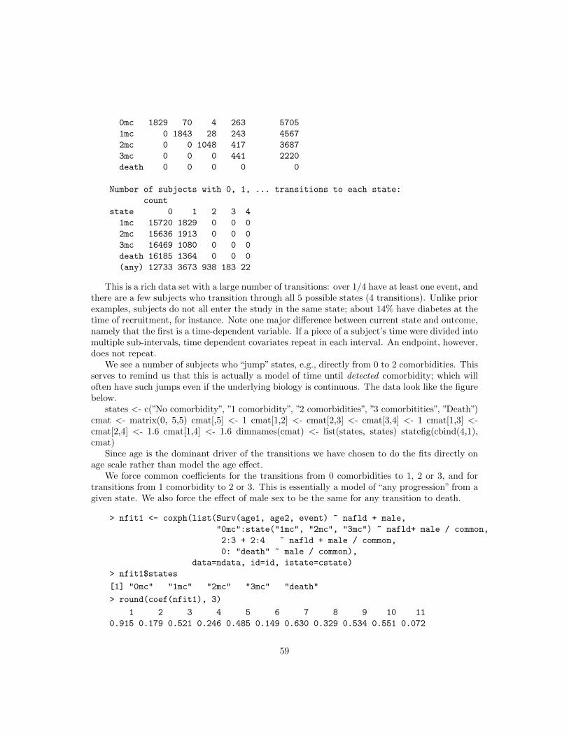
0mc 1829 70 4 263 5705

1mc 0 1843 28 243 4567

2mc 0 0 1048 417 3687

3mc 0 0 0 441 2220

death 0 0 0 0 0

Number of subjects with 0, 1, ... transitions to each state:

count

state 0 1 2 3 4

1mc 15720 1829 0 0 0

2mc 15636 1913 0 0 0

3mc 16469 1080 0 0 0

death 16185 1364 0 0 0

(any) 12733 3673 938 183 22

This is a rich data set with a large number of transitions: over 1/4 have at least one event, andthere are a few subjects who transition through all 5 possible states (4 transitions). Unlike priorexamples, subjects do not all enter the study in the same state; about 14% have diabetes at thetime of recruitment, for instance. Note one major difference between current state and outcome,namely that the first is a time-dependent variable. If a piece of a subject’s time were divided intomultiple sub-intervals, time dependent covariates repeat in each interval. An endpoint, however,does not repeat.

We see a number of subjects who “jump” states, e.g., directly from 0 to 2 comorbidities. Thisserves to remind us that this is actually a model of time until detected comorbidity; which willoften have such jumps even if the underlying biology is continuous. The data look like the figurebelow.

states <- c(”No comorbidity”, ”1 comorbidity”, ”2 comorbidities”, ”3 comorbitities”, ”Death”)cmat <- matrix(0, 5,5) cmat[,5] <- 1 cmat[1,2] <- cmat[2,3] <- cmat[3,4] <- 1 cmat[1,3] <-cmat[2,4] <- 1.6 cmat[1,4] <- 1.6 dimnames(cmat) <- list(states, states) statefig(cbind(4,1),cmat)

Since age is the dominant driver of the transitions we have chosen to do the fits directly onage scale rather than model the age effect.

We force common coefficients for the transitions from 0 comorbidities to 1, 2 or 3, and fortransitions from 1 comorbidity to 2 or 3. This is essentially a model of “any progression” from agiven state. We also force the effect of male sex to be the same for any transition to death.

> nfit1 <- coxph(list(Surv(age1, age2, event) ~ nafld + male,

"0mc":state("1mc", "2mc", "3mc") ~ nafld+ male / common,

2:3 + 2:4 ~ nafld + male / common,

0: "death" ~ male / common),

data=ndata, id=id, istate=cstate)

> nfit1$states

[1] "0mc" "1mc" "2mc" "3mc" "death"

> round(coef(nfit1), 3)

1 2 3 4 5 6 7 8 9 10 11

0.915 0.179 0.521 0.246 0.485 0.149 0.630 0.329 0.534 0.551 0.072

59

> nfit1$cmap

1:2 1:3 2:3 1:4 2:4 3:4 1:5 2:5 3:5 4:5

(Baseline) 1 2 3 4 5 6 7 8 9 10

nafld 1 1 3 1 3 5 7 9 10 11

male 2 2 4 2 4 6 8 8 8 8

A list has been used as the formula for the coxph call. The first element is a standardformula, and will be the default for all of the transitions found in the model. Elements 2–4 ofthe list are pseudo formulas, which specify a set of states on the left and covariates on the right,along with the optional modifier /common. As shown, there are multiple ways to specify a set oftransitions either by name or by number, the value 0 is shorthand for “any state”. A ’1’ on theright-hand side can be used to force a common baseline hazard for two transitions. A commonbaseline for two transitions that originate from the same state is incompatable with the Coxpartial likelihood, however, and will lead to multiple un-estimable coefficients.

Here are two forms of the printout. We limit the number of digits to better fit on thisdocument page.

> options(show.signif.stars = FALSE) # display statistical maturity

> print(summary(nfit1, digits =3))

Call:

coxph(formula = list(Surv(age1, age2, event) ~ nafld + male,

"0mc":state("1mc", "2mc", "3mc") ~ nafld + male/common, 2:3 +

2:4 ~ nafld + male/common, 0:"death" ~ male/common),

data = ndata, id = id, istate = cstate)

n= 22683, number of events= 6186

coef exp(coef) se(coef) robust se z Pr(>|z|)

1 0.91468 2.49598 0.06267 0.06737 13.578 < 2e-16

2 0.17895 1.19596 0.04625 0.04822 3.711 0.000206

3 0.52076 1.68331 0.05227 0.05584 9.327 < 2e-16

4 0.24559 1.27838 0.04702 0.04991 4.921 8.60e-07

5 0.48494 1.62408 0.06498 0.06788 7.145 9.02e-13

6 0.14900 1.16067 0.06250 0.06506 2.290 0.022020

7 0.62990 1.87742 0.22590 0.22793 2.764 0.005717

8 0.32935 1.39006 0.05488 0.05466 6.026 1.69e-09

9 0.53433 1.70630 0.15483 0.14971 3.569 0.000358

10 0.55116 1.73526 0.10585 0.10695 5.153 2.56e-07

11 0.07225 1.07492 0.09929 0.09908 0.729 0.465891

exp(coef) exp(-coef) lower .95 upper .95

1 2.496 0.4006 2.1872 2.848

2 1.196 0.8361 1.0881 1.315

3 1.683 0.5941 1.5088 1.878

4 1.278 0.7822 1.1593 1.410

5 1.624 0.6157 1.4218 1.855

60

6 1.161 0.8616 1.0217 1.319

7 1.877 0.5326 1.2010 2.935

8 1.390 0.7194 1.2488 1.547

9 1.706 0.5861 1.2724 2.288

10 1.735 0.5763 1.4071 2.140

11 1.075 0.9303 0.8852 1.305

Concordance= 0.569 (se = 0.004 )

Likelihood ratio test= 448.4 on 11 df, p=<2e-16

Wald test = 436.2 on 11 df, p=<2e-16

Score (logrank) test = 520.2 on 11 df, p=<2e-16, Robust = 326.7 p=<2e-16

(Note: the likelihood ratio and score tests assume independence of

observations within a cluster, the Wald and robust score tests do not).

> print(nfit1, digits =3)

Call:

coxph(formula = list(Surv(age1, age2, event) ~ nafld + male,

"0mc":state("1mc", "2mc", "3mc") ~ nafld + male/common, 2:3 +

2:4 ~ nafld + male/common, 0:"death" ~ male/common),

data = ndata, id = id, istate = cstate)

1:2 coef exp(coef) se(coef) robust se z p

nafld 0.9147 2.4960 0.0627 0.0674 13.58 < 2e-16

male 0.1790 1.1960 0.0462 0.0482 3.71 0.00021

1:3 coef exp(coef) se(coef) robust se z p

nafld 0.9147 2.4960 0.0627 0.0674 13.58 < 2e-16

male 0.1790 1.1960 0.0462 0.0482 3.71 0.00021

2:3 coef exp(coef) se(coef) robust se z p

nafld 0.5208 1.6833 0.0523 0.0558 9.33 < 2e-16

male 0.2456 1.2784 0.0470 0.0499 4.92 8.6e-07

1:4 coef exp(coef) se(coef) robust se z p

nafld 0.9147 2.4960 0.0627 0.0674 13.58 < 2e-16

male 0.1790 1.1960 0.0462 0.0482 3.71 0.00021

2:4 coef exp(coef) se(coef) robust se z p

nafld 0.5208 1.6833 0.0523 0.0558 9.33 < 2e-16

male 0.2456 1.2784 0.0470 0.0499 4.92 8.6e-07

61

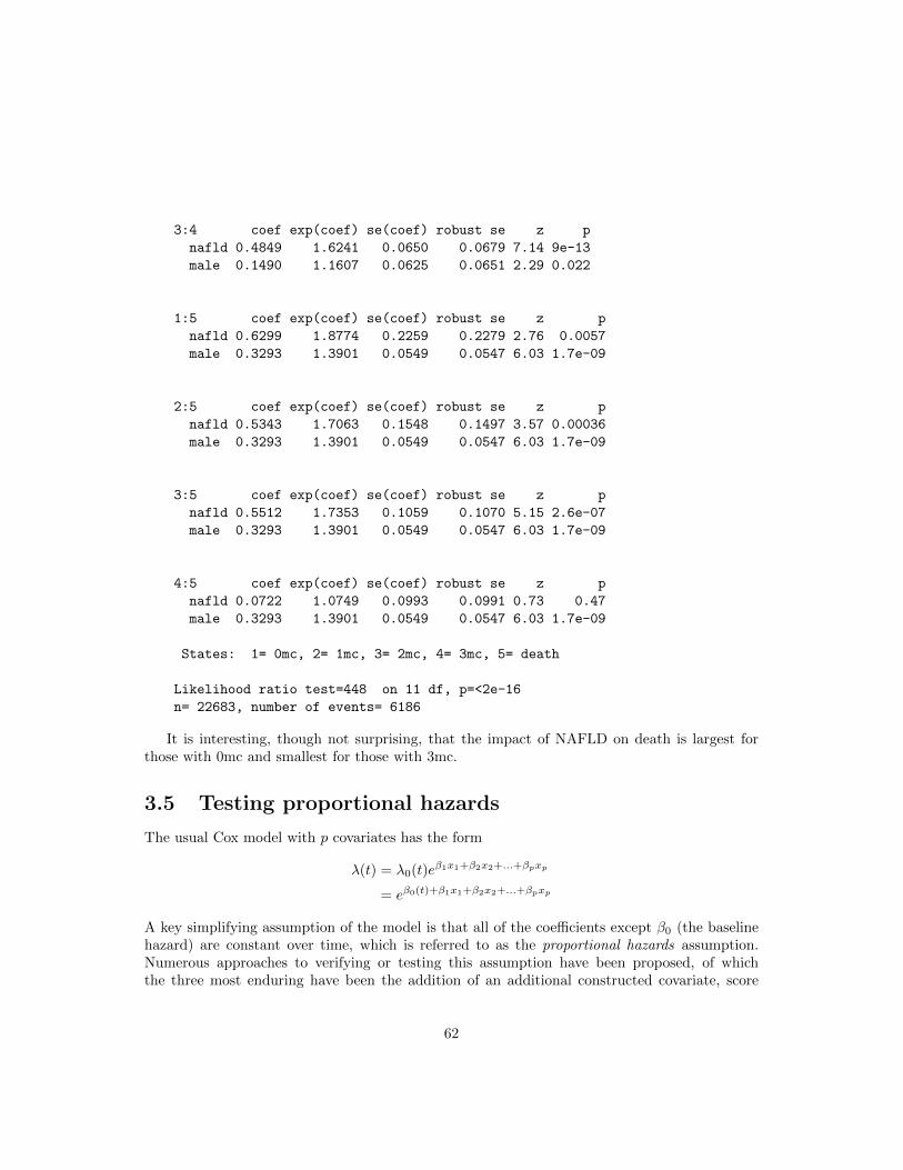
3:4 coef exp(coef) se(coef) robust se z p

nafld 0.4849 1.6241 0.0650 0.0679 7.14 9e-13

male 0.1490 1.1607 0.0625 0.0651 2.29 0.022

1:5 coef exp(coef) se(coef) robust se z p

nafld 0.6299 1.8774 0.2259 0.2279 2.76 0.0057

male 0.3293 1.3901 0.0549 0.0547 6.03 1.7e-09

2:5 coef exp(coef) se(coef) robust se z p

nafld 0.5343 1.7063 0.1548 0.1497 3.57 0.00036

male 0.3293 1.3901 0.0549 0.0547 6.03 1.7e-09

3:5 coef exp(coef) se(coef) robust se z p

nafld 0.5512 1.7353 0.1059 0.1070 5.15 2.6e-07

male 0.3293 1.3901 0.0549 0.0547 6.03 1.7e-09

4:5 coef exp(coef) se(coef) robust se z p

nafld 0.0722 1.0749 0.0993 0.0991 0.73 0.47

male 0.3293 1.3901 0.0549 0.0547 6.03 1.7e-09

States: 1= 0mc, 2= 1mc, 3= 2mc, 4= 3mc, 5= death

Likelihood ratio test=448 on 11 df, p=<2e-16

n= 22683, number of events= 6186

It is interesting, though not surprising, that the impact of NAFLD on death is largest forthose with 0mc and smallest for those with 3mc.

3.5 Testing proportional hazards

The usual Cox model with p covariates has the form

λ(t) = λ0(t)eβ1x1+β2x2+...+βpxp

= eβ0(t)+β1x1+β2x2+...+βpxp

A key simplifying assumption of the model is that all of the coefficients except β0 (the baselinehazard) are constant over time, which is referred to as the proportional hazards assumption.Numerous approaches to verifying or testing this assumption have been proposed, of whichthe three most enduring have been the addition of an additional constructed covariate, score

62

tests, and tests based on cumulative martingale sums. Each of these is normally applied to onecovariate at a time.

3.5.1 Constructed variables

For the constructed variable approach, assume that the true form of the model for variable x1is β1(t)x1, with the coefficient having the simple linear form β1(t) = a+ bt. Then

β1(t)x1 = ax1 + b(x1t)

= ax1 + bz (3.4)

that is, we can create a special time-dependent covariate z = x1t, add add it to the data set,and then use an ordinary coxph fit.

Consider the veterans lung cancer data set, which has often been used to illustrate non-proportional hazards. Adding this special covariate is not quite as simple as writing

> fit2 <- coxph(Surv(time, status) ~ trt + trt*time + celltype + karno,

data = veteran)

The problem is that time is trying to play two roles in the above equation, the final follow-uptime for each subject and the continuous time scale t of equation (3.4). The solution to to createthe special variable explicitly before calling the regression function. Since the Cox model addsa term to the likelihood at each unique death time, it is sufficient to create a data set with thesame granularity.

> dtime <- unique(veteran$time[veteran$status==1]) # unique times

> newdata <- survSplit(Surv(time, status) ~ trt + celltype + karno,

data=veteran, cut=dtime)

> nrow(veteran)

[1] 137

> nrow(newdata)

[1] 5959

> fit0 <- coxph(Surv(time, status) ~ trt + celltype + karno, veteran)

> fit1 <- coxph(Surv(tstart, time, status) ~ trt + celltype + karno,

data=newdata)

> fit2 <- coxph(Surv(tstart, time, status) ~ trt + celltype + karno +

time:karno, newdata)

> fit2

Call:

coxph(formula = Surv(tstart, time, status) ~ trt + celltype +

karno + time:karno, data = newdata)

coef exp(coef) se(coef) z p

trt 1.686e-01 1.184e+00 2.048e-01 0.823 0.41034

celltypesmallcell 8.990e-01 2.457e+00 2.746e-01 3.274 0.00106

celltypeadeno 1.192e+00 3.293e+00 2.991e-01 3.985 6.74e-05

63

celltypelarge 4.034e-01 1.497e+00 2.833e-01 1.424 0.15454

karno -4.015e-02 9.606e-01 6.383e-03 -6.291 3.16e-10

karno:time 1.110e-04 1.000e+00 4.688e-05 2.369 0.01784

Likelihood ratio test=66.92 on 6 df, p=1.75e-12

n= 5959, number of events= 128

> fit2b <- coxph(Surv(tstart, time, status) ~ trt + celltype + karno +

rank(time):karno, newdata)

The fits give a warning message about the use of the time variable on both sides of theequation, since two common cases where time appears on both sides are the naive model shownfurther above and frank typing mistakes. In this particular case we can ignore the warning sincethe data set was carefully constructed for this special purpose, but it should never be treatedcasually.

Alternatively, coxph has built-in functionality that will build the expanded data set for us,behind the scenes, and then use that expanded data for the fit. Here is eqivalent code to testthe Karnofsky variable:

> fit2 <- coxph(Surv(tstart, time, status) ~ trt + celltype + karno +

tt(karno), data =newdata,

tt = function(x, t,...) x*t)

There are 4 issues with the constructed variable approach.

1. The choice β(t) ≈ a+ bt was arbitrary. Perhaps the true form is a+ b log(t) (fit2b above),or some other function.

2. The intermediate data set can become huge. It will be of order O(nd) where d is thenumber of unique event times, and d grows along with n.

3. The coefficients for a factor variable such as celltype can be confusing, since the resultsdepend on how the 0/1 indicators for the variable are chosen.

4. Outliers in time are an issue. The veteran cancer data set, for instance, contains a time of999 days (a particularly suspicious value in any data set). The Cox model itself dependsonly on the rank order of the event times, so such outliers are not an issue for the basemodel, but as a covariate these values can have undue influence. The time-dependentcoeffient for Karnofsky has p < .01 in fit2b above, which uses rank(time), a change that islargely due to dampening the leverage of outliers.

3.5.2 Score tests

The cox.zph function checks proportional hazards for a fitted Cox model directly, and tries toaddress the four issues discussed above.

� It is easy to specify alternate time transforms such as x*log(t). More importantly, the codeproduces both a diagnostic plot that suggests the shape of any non-proportionality, alongwith a test of the chosen time-transform.

64

� The test statistic is based on a score test, which does not require creating the expandeddata set.

� Multi-covariate terms such as a factor or splines are by default treated as a single effect.

� The default time transform is designed to minimize outliers in time.

Shown below are results for the veterans data using fit0 from above. The score statistic forthe simple term x*time (zp1) closely matches the Wald test for the full time dependent fit foundin fit2 above, which is what we would expect; score, Wald and likelihood ratio tests usuallyagree quite closely for Cox models.

> zp0 <- cox.zph(fit0, transform='identity')

> zp0

chisq df p

trt 0.00493 1 0.94402

celltype 18.41391 3 0.00036

karno 6.05160 1 0.01389

GLOBAL 20.87086 5 0.00086

> zp1 <- cox.zph(fit0, transform='log')

> zp1

chisq df p

trt 0.215 1 0.64298

celltype 13.586 3 0.00353

karno 10.079 1 0.00150

GLOBAL 21.451 5 0.00067

> oldpar <- par(mfrow=c(2,2))

> for (i in 1:3) {plot(zp1[i]); abline(0,0, lty=3)}

> plot(zp0[3])

> par(oldpar)

65

1 5 10 50 500

−3

−1

01

23

Time

Bet

a(t)

for

trt ●

●

●

●● ●

●●

●

●

●

●

●●

●

●●●

●

●●

●●●

●●●

●

●

●

●

●

●●●●●

●

●

●

●

●

●●

●

●

●

●●

●●●

●

●●

●

●●●

●●●

●

●

●

●

●●●

●

●●●

●●

●●●

●●●●

●●●

●●

●●●●

●

●

●

●●●●●●●

●

●

●

●

●

●●

●●

●●●

●

●

●

●●●

●

●

●

●

●

●

● ●●

1 5 10 50 500

−4

02

46

Time

Bet

a(t)

for

cellt

ype

●●

●

●

● ●●

●

●

●●

●

●

●

●

●

●

●●

●

●

●●●

●●

●

●●●●●●

●

●

●●●●●

●

●

●

●

●

●

●

●

●

●●

●

●●

●

●

●

●●

●●●

●

●

●

●

●

●

●

●

●

●

●●●

●●●

●●●

●●

●

●

●

●

●

●

●

●

●

●

●

●

●

●●

●

●

●●

●

●

●

●

●

●

●

●

●●●

●

●

●

●

●

●

●

●

●

●●

●

● ●●

1 5 10 50 500

−0.

15−

0.05

0.05

Time

Bet

a(t)

for

karn

o

●

●

●

●

●

●

●

●●

●

●

●

●

●

●

●

●

●

●

●

●

●

●

●

●

●

●●●

●

●

●●

●

●

●

●

●

●

●●

●●

●

●

●

●●●

●

●

●

●

●

●

●

●●●

●

●

●

●

●

●●●

●

●

●

●

●●

●

●

●●

●

●

●●●

●

●

●

●●

●

●

●

●

●

●

●

●

●

●

●

●

●●

●

●

●

●●

●

●

●

●

●

●

●

●

●

●

●

●

●

●

●

●

●

●

●

● ●

●

0 200 400 600 800 1000

−0.

15−

0.05

0.05

Time

Bet

a(t)

for

karn

o

●

●

●

●

●

●

●

●●

●

●

●

●

●

●

●

●

●

●

●

●

●

●

●

●

●

●●●

●

●

●●

●

●

●

●

●

●

●●

●●

●

●

●

●●●

●

●

●

●

●

●

●

●●●

●

●

●

●

●

●●●

●

●

●

●

●●

●

●

●●

●

●

●●●

●

●

●

●●

●

●

●

●

●

●

●

●

●

●

●

●

●●

●

●

●

●●

●

●

●

●

●

●

●

●

●

●

●

●

●

●

●

●

●

●

●

● ●

●

A test for zero slope, from a least squares regression using data in the matching plot approx-imates the score test. (In versions of the package prior to survival3.0, the approximate test wasused for the formal printout and test as well.) If proporitional hazard holds we would expectthe fitted line to be horizontal, i.e., β(t) is constant. Rather than show a fitted line the plotadds a general smooth curve, which can help reveal the form of non-proportional hazards, ifit exists. The first three panels of the plot show curves for the three covariates on a log(time)scale. Since celltype is a factor, the plot shows the time dependent effect of the portion of thelinear predictor associated with cell type; if proportional hazards is true wrt that term a fittedline should be horizontal with a coefficient of 1. The effect of Karnofsky score appears becomeessentially 0 after approximately 6 months; for this cohort of subjects with advanced lung cancer,a 6 month old assessment is no longer relevant. The corresponding plot in the lower right panel,however, shows that the outlier time of 999 days has an undue influence on any such regression.A test of proportional hazards on that scale must also be treated with caution. The plot usinglog scale lacks these outliers and is more interpretable.

The default time transform is based on a Kaplan-Meier transform, i.e., that monotone trans-form of the time axis that will cause the KM plot to be a straight line. This is a good default forthe score tests, since it essentially guarrantees that there wil be no outliers in the constructedxg(time), while dealing with censoring in a defensible way. That is, the code has opted for asafe default. It is not as easily interpreted as other scales for the plots, however.

The cox.zph function does not attempt a score test for random effects (frailty) terms, infact is not clear what the computation for such a test should be. The function will check othercovariates in a model that contains a random effect, however; the estimated random effect per

66

subject is essentially treated as a fixed offset.

67

Chapter 4

Accelerated Failure Time models

68

Chapter 5

Tied event times

5.1 Cox model estimates

The theory for the Cox model has always been worked out for the case of continuous time, whichimplies that there will be no tied event or censoring times in the data set. With respect tocensoring times, all of the survival library commands treat censoring as occuring “just after” therecorded time point. The rationale is that if a subject was last observed alive on day 231, say,then their death time, whatever it is, must be strictly greater than 231. For formally, a subjectwho was censored at time t is considered to have been at risk for any events that occured at timet.

The issue with tied event times is more complex, and the software supports three differentalgorithms for dealing with this. The Cox partial likelihood is a sum of terms, one for eachevent time, each of which compares the subject who had the event to the set of subjects who“could have had the event”: the risk set. The overall view is essentially a lottery model: at eachevent time there was a drawing to select one subject for the event, the risk score for each subjectexp(Xiβ) tells how many “tickets” each subject had in the drawing. The software implementsthree different algorithms for dealing with tie event times.

The Breslow approximation (ties=’breslow’) in essence ignores the ties. If two subjects Aand B died on day 100, say, the partial likelihood will have separate terms for the two deaths.Subject A will be at risk for the death that happened to B, and B will be at risk for the deaththat happened to A. In life this is not technically possible of course: whoever died first will notbe at risk for the second death.

The Efron approximation can be motivated by the idea of coarsening : time is on a continuousscale but we only observe a less precise version of it. For example consider the acute myelogenousleukemia data set that is part of the package, which was a clinical trial to test if extendendchemotherapy (“Maintained”) was superior to standard. The time to failure was recorded inmonths, and in the non-maintained arm there are two pairs of failures, at 5 and at 8 months. Itmight be reasonable to assume that if the data had been recored in days these ties might nothave occured.

> with(subset(aml, x=="Nonmaintained"), Surv(time, status))

[1] 5 5 8 8 12 16+ 23 27 30 33 43 45

69

Let the risk scores exp(Xβ) for the 12 subjects be r1–r12, and assume that the two failuresactually at month 5 are not tied on a finer time scale. For the first event, whichever it is, the riskset with be all subjects 1–12 and the denominator of the partial likelihood term is

∑ri. For the

second event, the denominator is either r1+r3+. . . r12 or r2+r3+. . . r12; the Efron approximationis to use the average of the two as the denominator term. In the software this is easily doneby using temporary case weights: if there were k tied events then one of the denomiators giveseach of those k subjects a weight of 1, then next gives each a weight of (k − 1)/k, then next aweight of (k−2)/k, etc. The Efron approximation imposes a tiny bit more bookkeeping, but thethe computational burden is no different that for case weights; i.e., it effectively takes no morecomputational time than the Breslow approximation.

The third possiblility is the exact partial likelihood due to Cox, which treats the underlyingtime scale as discrete rather than continuous. When taking this view the denominator of thepartial likelihood term is again an average, but over a much larger subset. If there are k eventsand n subjects at risk, the EPL sum is over all k choose n possible choices. In the AML exampleabove, the event at time 5 will be a sum over 12(11)/2= 33 terms. If the number of ties is largethis quickly grows unreasonable: for 20 ties out of 1000 the sum has over 39 billion terms. Aclever algorithm by Gail makes this sum barely possible, but it does not extend to the case of(tstart, tstop) style data.

An important aside is that the log-likelihood for matched logistic regression is identical tothe Cox partial likelihood for a particular data set, when the EPL is used. Namely, set time=1(or any other constant), status = 0 for controls and 1 for cases, and fit a coxph model with eachmatched set as a separate stratum. In most instances a matched set will consist of a single casealong with one or more controls, however, which is the case where the Breslow, Efron, and EPLare identical. (The EPL will still take slightly longer to run due to setting up the necessarystructure for all those sums.)

How important are the ties, actually? Below we show a small computation in which a largerdata set is successively coarsened and compare the results. The colon cancer data set has 929subjects with stage B/C colon cancer who were randomized to three treatment arms and thenfollowed for 5 years; the time to death or progression is in days. In the example below wesuccessively coarsen the time scale to be monthly, bimonthly, . . . , bi-annual; the last of whichgenerates an very large number of ties. What we see is that

� The Efron approximation is quite good at dealing with the coarsened data, producingnearly the same coefficient as the original data even when the coarsening is extreme.

� The Breslow approximation is biased somewhat towards 0, the exact paritial likelihoodsomewhat away from 0.

� The differences are very small. With monthly coarsening, which is itself fairly large, the 3estimates differ by about .01 while the standard error of the original coefficient is 0.96; i.e.a shift that is statistically immaterial.

> tdata <- subset(colon, etype==1) # progression or death

> cmat <- matrix(0, 7, 6)

> for( i in 1:7) {

if (i==1) scale <-1 else scale <- (i-1)*365/12

70

temp <- floor(tdata$time/scale)

tfit <- coxph(Surv(temp, status) ~ node4 + extent, tdata)

tfit2 <- coxph(Surv(temp, status) ~ node4 + extent, tdata,

ties='breslow')

tfit3 <- coxph(Surv(temp, status) ~ node4 + extent, tdata,

ties='exact')

cmat[i,] <- c(coef(tfit2), coef(tfit), coef(tfit3))

}

> matplot(1:7, cmat[,c(1,3,5)], xaxt='n', pch='bec',

xlab="Time divisor", ylab="Coefficient for node4")

> axis(1, 1:7, c(1, floor(1:6 *365/12)))

b

b

bb

b b

b0.78

0.80

0.82

0.84

0.86

0.88

Time divisor

Coe

ffici

ent f

or n

ode4

e e e e e

e

e

cc

c

cc

c

c

1 30 60 91 121 152 182

Early on in the package the decision was made to make the Efron approximation the default.The reasoning was simply that is is more accurate, even if only a little, and the author’s earlybackground in numerical analysis argued strongly to always use the best approximation available.The second reason is that the computational cost is low. Most of us would pick up a 1 Eurocoin on the sidewalk, even though it will not make any real change in our income. One downsideis that no other package did this, leading to a very common complaint/question that R “givesdifferent results”. A second is that it leads to further downstream programming as discussed infollowing sections.

71

5.2 Cumulative hazard and survival

The coarsening argument can also be applied to the cumulative hazard Λ(t). Say that therewere 3 deaths with 10 subjects at risk. The increment to the Nelson-Aalen cumulative hazardestimate would then be 3/10. If the data had been observed in continuous time, however, therewould have been 3 increments of 1/10 + 1/9 + 1/8. This estimate was explored by Fleming andHarrington [2]. In the survfit function the ctype option selects for 1=Nelson-Aalen and 2=Fleming-Harrington.

The Kaplan-Meier estimate is not subject to the coarsening phenominon. In our example, theobserved data will lead to a multipilicative increment of 7/10 and the continuous data to one of(9/10)(8/9)(7/8), which are the same. An alternate estimate of the survival is S(t) = exp(−Λ(t)).Basing this on the FH estimate of hazard will more closely track the KM when there are tied eventtimes. The direct (KM) vs. exponential estimates of survival are obtained with the ctype=1 andctype=2 arguments; however, the exponential estimate is quite uncommon outside of the Coxmodel.

5.3 Predicted cumulative hazard and surival from a Coxmodel

Predictions from a coxph model must always be for someone, i.e., some particular set of covariatevalues. Let ri = exp(Xiβ − c) be the recentered risk scores for each subject i, where the

recentering constant c = Xnβ, Xn being the covariates of the “new” subject for which predictionis desired. (We don’t want to create a prediction for a baseline subject with X=0, what textbooksoften call a “baseline hazard”, since if 0 is too far from the center of the data the exp functioncan easily overflow.) The estimated cumulative hazard at any event time is then

Λ(t) =

∫ t

0

∑i dNi(t)∑i Yi(t)ri

(5.1)

Equation (5.1) is known as the Breslow estimate; if β = 0 then ri = 1 and it becomes equal tothe Nelson-Aalen estimator.

If the Efron estimate is used for ties, then the software uses an Efron estimate of the cumula-tive hazard; which reduces to the Fleming-Harrington if β = 0. Using the hazard estimate thatmatches the parial likelihood estimate causes an important property of the vector of martingaleresiduals m to hold, namely that mX is equal to the first derivative of the partial likelihood.residuals hold for both

The Cox model is a case where the default estimate of survival is based on the exponent ofthe cumulative hazard, rather than a ’direct’ one such as the Kaplan-Meier. There are threereasons for this.

1. The most obvious ’direct’ estimate is to use (∑dNi(t)−

∑Yi(t)ri)/(

∑Yi(t)ri) as a mul-

tiplicative update at each event time t. This expression in not guarranteed to be between0 and 1, however, particular for new subjects who are near or past the boundaries of theoriginal data set. This leads to using some sort of ad hoc correction to avoid failure.

72

2. The direct estimate of Kalbfleisch and Prentice avoids this, but it does not extend todelayed entry, multi-state models or other extensions of the basic model.

3. The KP estimate reqires iteration so the code is more complex.

5.4 Multi-state models

Multi-state hazards models have a very interesting (and useful) property, which is that hazardscan be estimated singly (without reference to any other transition) but probability-in-state esti-mators must be computed globally. Thus, one can estimate non-parametric cumulative hazardestimates (Nelson-Aalen), the hazard ratios for any given transtion (Cox model) or the predictedcumulative hazard function based on a per transition Cox model without incurring any issueswith respect to competing risks. (If there is informative censoring the overall and individual es-timates still agree, but they will both be wrong. An example of informative censoring would besubjects who are removed from the data because of an impending event, e.g., censoring subjectswho enter hospice care would underestimate death rates.)

Now say that we had a simple competing risks problem, 10 subjects are alive and in theinitial state on day 100, at which time two of them transition to two different endpoints. Acoarsening argument would say that on the underlying continuous time scale these two subjectswould not be tied, and then would use 9.5 as the denominator for each of the two cumulativehazard increments. Such an estimate would however then be at variance with the two indiviuallycomputed hazards: global coarsening removes the separability. The survival package takes amoderated view and will apply the coarsening argument separately to each hazard, i.e., it choseto retain the separation policy.

5.5 Parametric Regression

5.5.1 Usage

The survreg function implements the class of parametric accelerated failure time models. As-sume that the survival time y satisfies log(y) = X ′β + σW , for W from some given distribution.Then if Λw(t) is the cumulative hazard function for W , the cumulative hazard function for sub-ject i is Λw[exp(−ηi/σ)t], that is, the time scale for the subject is accelerated by a constantfactor. A good description of the models is found in chapter 3 of Kalbfleisch and Prentice [4].

The following fits a Weibull model to the lung cancer data set included in the package.

> fit <- survreg(Surv(time, status) {\twiddle} age + sex + ph.karno, data=lung,

dist='weibull')

> fit

Call:

survreg(formula = Surv(time, status) {\twiddle} age + sex + ph.karno, data = lung, dist

= "weibull")

Coefficients:

(Intercept) age sex ph.karno

5.326344 -0.008910282 0.3701786 0.009263843

73

Scale= 0.7551354

Loglik(model)= -1138.7 Loglik(intercept only)= -1147.5

Chisq= 17.59 on 3 degrees of freedom, p= 0.00053

n=227 (1 observations deleted due to missing)

The code for the routines has undergone substantial revision between releases 4 and 5 ofthe code. Calls to the older version are not compatable with all of the changes, users canuse the survreg.old function if desired, which retains the old argument style (but uses thenewer maximization code). Major additions included penalzed models, strata, user specifieddistributions, and more stable maximization code.

5.5.2 Strata

In a Cox model the strata statement is used to allow separate baseline hazards for subgroupsof the data, while retaining common coefficients for the other covariates across groups. Forparametric models, the statement allows for a separate scale parameter for each subgroup, butagain keeping the other coefficients common across groups. For instance, assume that separate“baseline” hazards were desired for males and females in the lung cancer data set. If we think ofthe intercept and scale as the baseline shape, then an appropriate model is

> sfit <- survreg(Surv(time, status) ~ sex + age + ph.karno + strata(sex),

data=lung)

> sfit

Coefficients:

(Intercept) sex age ph.karno

5.059089 0.3566277 -0.006808082 0.01094966

Scale:

sex=1 sex=2

0.8165161 0.6222807

Loglik(model)= -1136.7 Loglik(intercept only)= -1146.2

Chisq= 18.95 on 3 degrees of freedom, p= 0.00028

The intercept only model used for the likelihood ratio test has 3 degrees of freedom, correspondingto the intercept and two scales, as compared to the 6 degrees of freedom for the full model.

This is quite different from the effect of the strata statement in censorReg; there it acts asa ‘by’ statement and causes a totally separate model to be fit to each gender. The same fit (butnot as nice a printout) can be obtained from survreg by adding an explicit interaction to theformula:

Surv(time,status) ~ sex + (age + ph.karno)*strata(sex)

74

5.5.3 Penalized models

Let the linear predictor for a survreg model be η = Xβ + Zω, and consider maximizing thepenalized log-likelihood

PLL = LL(y;β, ω)− p(ω; θ) ,

where β and ω are the unconstrained effects, respectively, X and Z are the covariates, p is afunction that penalizes certain choices for ω, and θ is a vector of tuning parameters.

For instance, ridge regression is based on the penalty p = θ∑ω2j ; it shrinks coefficients

towards zero.The penalty functions in survreg currently use the same code as those for coxph. This works

well in the case of ridge and pspline, but frailty terms are more problematic in that the codeto automatically choose the tuning parameter for the random effect no longer solves an MLEequation. More work on understanding these models is needed.

5.5.4 Specifying a distribution

The fitting routine is quite general, and can accept any distribution that spans the real linefor W , and any monotone transformation of y. The standard set of distributions is containedin a list survreg.distributions. Elements of the list are of two types. Basic elements are adescription of a distribution. Here is the entry for the logistic family:

logistic = list(

name = "Logistic",

variance = function(parm) pi^2/3,

init = function(x, weights, ...) \{

mean <- sum(x*weights)/ sum(weights)

var <- sum(weights*(x-mean)^2)/ sum(weights)

c(mean, var/3.2)

\},

deviance= function(y, scale, parms) \{

status <- y[,ncol(y)]

width <- ifelse(status==3,(y[,2] - y[,1])/scale, 0)

center <- y[,1] - width/2

temp2 <- ifelse(status==3, exp(width/2), 2) #avoid a log(0) message

temp3 <- log((temp2-1)/(temp2+1))

best <- ifelse(status==1, -log(4*scale),

ifelse(status==3, temp3, 0))

list(center=center, loglik=best)

\},

density = function(x, ...) \{

w <- exp(x)

cbind(w/(1+w), 1/(1+w), w/(1+w)^2, (1-w)/(1+w), (w*(w-4) +1)/(1+w)^2)

\},

quantile = function(p, ...) log(p/(1-p))

)

� Name is used to label the printout.

75

� Variance contains the variance of the distribution. For distributions with an optionalparameter such as the t-distribution, the parm argument will contain those parameters.

� Deviance gives a function to compute the deviance residuals. More on this is explainedbelow in the mathematical details.

� The density function gives the necessary quantities to fit the distribution. It should returna matrix with columns F (x), 1−F (x), f(x), f ′(x)/f(x) and f ′′(x)/f(x), where f ′ and f ′′

are the first and second derivatives of the density function, respectively.

� The quantiles function returns quantiles, and is used for residuals.

The reason for returning both F and 1 − F in the density function is to avoid round off errorwhen F (x) is very close to 1. This is quite simple for symmetric distributions, in the Gaussiancase for instance we use qnorm(x) and qnorm(-x) respectively. (In the intermediate steps ofiteration very large deviates may be generated, and a probabilty value of zero will cause furtherproblems.)

Here is an example of the second type of entry:

exponential = list(

name = "Exponential",

dist = "extreme",

scale =1 ,

trans = function(y) log(y),

dtrans= function(y) 1/y ,

itrans= function(x) exp(x)

)

This states that an exponential fit is computed by fitting an extreme value distribution to the logtransformation of y. (The distribution pointed to must not itself be a pointer to another). Theextreme value distribution is restricted to have a scale of 1. The first derivative of the transfor-mation, dtrans, is used to adjust the final log-likelihood of the model back to the exponential’sscale. The inverse transformation itrans is used to create predicted values on the original scale.

The formal rules for an entry are that it must include a name, either the “dist” componentor the set “variance”,“init”, “deviance”, “density” and “quantile”, an optional scale, and either allor none of “trans”, “dtrans” and “itrans”.

The dist="weibull" argument to the survreg function chooses the appropriate list fromthe survreg.distributions object. User defined distributions of either type can be specified bysupplying the appropriate list object rather than a character string. Distributions should, ingeneral, be defined on the entire real line. If not the minimizer used is likely to fail, since it hasno provision for range restrictions.

Currently supported distributions are

� basic

– (least) Extreme value

– Gaussian

– Logistic

76

– t-distribution

� transformations

– Exponential

– Weibull

– Log-normal (’lognormal’ or ’loggaussian’)

– Log-logistic (’loglogistic’)

5.5.5 Residuals

Response

The target return value is y− y, but what should we use for y when the observation is not exact?We will let y0 be the MLE for the location parameter µ over a data set with only the observationof interest, with σ fixed at the solution to the problem as a whole, subject to the constraint thatµ be consistent with the data. That is, for an observation right censored at t = 20, we constainµ ≥ 20, similarly for left censoring, and constrain µ to lie within the two endpoints of an intervalcensored observation. To be consistent as the width of an interval censored observation goes tozero, this definition does require that the mode of the density lies at zero.

For exact, left, and right censored observations y0 = y, so that this appears to be an ordinaryresponse residual. For interval censored observations from a symmetric distribution, y0 = thecenter of the censoring interval. The only unusual case, then, is for a non-symmetric distributionsuch as the extreme value. As shown later in the detailed information on distributions, for theextreme value distribution this occurs for y0 = yl − log(b/[exp(b)− 1]), where b = yu − yl is thelength of the interval.

Deviance

Deviance residuals are response residuals, but transformed to the log-likelihood scale.

di = sign(ri)√LL(yi, y0;σ)− LL(yi, ηi;σ)

The definition for y0 used for response residuals, however, could lead to the square root of anegative number for left or right censored observations, e.g., if the predicted value for a rightcensored observation is less than the censoring time for that observation. For these observationswe let y0 be the unconstrained maximum, which leads to yhat0 = −∞ and +∞ for right andleft censored observations, respectively, and a log-likelihood term of 0.

The advantages of these residuals for plotting and outlier detection are nicely detailed inMcCullagh and Nelder [7]. However, unlike GLM models, deviance residuals for interval censoreddata are not free of the scale parameter. This means that if there are interval censored datavalues and one fits two models A and B, say, that the sum of the squared deviance residuals formodel A minus the sum for model B is not equal to the difference in log-likelihoods. This is onereason that the current survreg function does not inherit from class glm: glm models use thedeviance as the main summary statistic in the printout.

77

Dfbeta

The dfbeta residuals are a matrix with one row per subject and one column per parameter.The ith row gives the approximate change in the parameter vector due to observation i, i.e.,the change in β when observation i is added to a fit based on all observations but the ith.The dfbetas residuals scale each column of this matrix by the standard error of the respectiveparameter.

Working

As shown in section 5.5.7 below, the Newton-Raphson iteration used to solve the model can beviewed as an iteratively reweighted least squares problem with a dependent variable of “currentprediction - correction”. The working residual is the correction term.

Likelihood displacement residuals

Escobar and Meeker [1] define a matrix of likelihood displacement residuals for the acceleratedfailure time model. The full residual information is a square matrix A, with dimension thenumber of pertubations considered. Three examples are developed in detail, all with dimensionn, the number of observations.

Case weight pertubations measure the overall effect on the parameter vector of dropping acase. Let V be the variance matrix of the model, and L the n by p matrix with elements ∂Li/∂βj ,

where Li is the likelihood contribution of the ith observation. Then A = LV L′. The residualsfunction returns the diagonal values of the matrix. Note that LV equals the dfbeta residuals.

Response pertubations correspond to a change of 1 σ unit in one of the response values. Fora Gaussian linear model, the equivalent computation yields the diagonal elements of the hatmatrix.

Shape pertubations measure the effect of a change in the log of the scale parameter by 1 unit.The matrix residual type returns the raw values that can be used to compute these and other

LD influence measures. The result is an n by 6 matrix, containing columns for

Li∂Li∂ηi

∂2Li∂η2i

∂Li∂ log(σ)

∂Li∂ log(σ)2

∂2Li∂η∂ log(σ)

5.5.6 Predicted values

Linear predictor and response

The linear predictor is ηi = x′iβ, where xi is the covariate vecor for subject i and β is the finalparameter estimate. The standard error of the linear predictor is x′iV xi, where V is the variance

matrix for β.The predicted response is identical to the linear predictor for fits to the untransformed dis-

tributions, i.e., the extreme-value, logistic and Gaussian. For transformed distributions such asthe Weibull, for which log(y) is from an extreme value distribution, the linear predictor is on thetransformed scale and the response is the inverse transform, e.g. exp(ηi) for the Weibull. Thestandard error of the transformed response is the standard error of ηi, times the first derivativeof the inverse transformation.

78

Terms

Predictions of type terms are useful for examination of terms in the model that expand intomultiple dummy variables, such as factors and p-splines. The result is a matrix with one columnfor each of the terms in the model, along with an optional matrix of standard errors. Here is anexample using psplines on the 1980 Stanford data

> fit <- survreg(Surv(time, status) ~ pspline(age, df=3) + t5, stanford2,

dist='lognormal')

> tt <- predict(fit, type='terms', se.fit=T)

> yy <- cbind(tt$fit[,1], tt$fit[,1] -1.96*tt$se.fit[,1],

tt$fit[,1] +1.96*tt$se.fit[,1])

> matplot(stanford2$age, yy, type='l', lty=c(1,2,2))

> plot(stanford2$age, stanford2$time, log='y',

xlab='Age', ylab='Days', ylim=c(.1, 10000))

> matlines(stanford2$age, exp(yy+ attr(tt$fit, 'constant')), lty=c(1,2,2))

The second plot puts the fit onto the scale of the data, and thus is similar in scope to figure 1 inEscobar and Meeker [1]. Their plot is for a quadratic fit to age, and without T5 mismatch scorein the model.

Quantiles

If predicted quantiles are desired, then the set of probability values p must also be given to thepredict function. A matrix of n rows and p columns is returned, whose ij element is the pjthquantile of the predicted survival distribution, based on the covariates of subject i. This can bewritten as Xβ + zqσ where zq is the qth quantile of the parent distribution. The variance of thequantile estimate is then cV c′ where V is the variance matrix of (β, σ) and c = (X, zq).

In computing confidence bands for the quantiles, it may be preferable to add standard errorson the untransformed scale. For instance, consider the motor reliability data of Kalbfleisch andPrentice [5].

> fit <- survreg(Surv(time, status) ~ temp, data=motors)

> q1 <- predict(fit, data.frame(temp=130), type='quantile',

p=c(.1, .5, .9), se.fit=T)

> ci1 <- cbind(q1$fit, q1$fit - 1.96*q1$se.fit, q1$fit + 1.96*q1$se.fit)

> dimnames(ci1) <- list(c(.1, .5, .9), c("Estimate", "Lower ci", "Upper ci"))

> round(ci1)

Estimate Lower ci Upper ci

0.1 15935 9057 22812

0.5 29914 17395 42433

0.9 44687 22731 66643

> q2 <- predict(fit, data.frame(temp=130), type='uquantile',

p=c(.1, .5, .9), se.fit=T)

> ci2 <- cbind(q2$fit, q2$fit - 1.96*q2$se.fit, q2$fit + 1.96*q2$se.fit)

> ci2 <- exp(ci2) #convert from log scale to original y

79

> dimnames(ci2) <- list(c(.1, .5, .9), c("Estimate", "Lower ci", "Upper ci"))

> round(ci2)

Estimate Lower ci Upper ci

0.1 15935 10349 24535

0.5 29914 19684 45459

0.9 44687 27340 73041

Using the (default) Weibull model, the data is fit on the log(y) scale. The confidence bandsobtained by the second method are asymmetric and may be more reasonable. They are alsoguarranteed to be > 0.

This example reproduces figure 1 of Escobar and Meeker [1].

> plot(stanford2$age, stanford2$time, log='y',

xlab='Age', ylab='Days', ylim=c(.01, 10^6), xlim=c(1,65))

> fit <- survreg(Surv(time, status) ~ age + age^2, stanford2,

dist='lognormal')

> qq <- predict(fit, newdata=list(age=1:65), type='quantile',

p=c(.1, .5, .9))

> matlines(1:65, qq, lty=c(1,2,2))

Note that the percentile bands on this figure are really quite a different object than theconfidence bands on the spline fit. The latter reflect the uncertainty of the fitted estimate andare related to the standard error. The quantile bands reflect the predicted distribution of asubject at each given age (assuming no error in the quadratic estimate of the mean), and arerelated to the standard deviation of the population.

5.5.7 Fitting the model

With some care, parametric survival can be written so as to fit into the iteratively reweightedleast squares formulation used in Generalized Linear Models of McCullagh and Nelder [7]. Adetailed description of this setup for general maximum likelihood computation is found in Green[3].

Let y be the data vector (possibly transformed), and xi be the vector of covariates for theith observation. Assume that

zi ≡yi − x′iβ

σ∼ f

for some distribution f , where y may be censored.Then the likelihood for y is

l =

( ∏exact

f(zi)/σ

)∏right

∫ ∞zi

f(u)du

∏left

∫ zi

−∞f(u)du

( ∏interval

∫ zui

zli

f(u)du

),

where “exact”, “right”, “left”, and “interval” refer to uncensored, right censored, left censored,and interval censored observations, respectively, and zli, z

ui are the lower and upper endpoints,

respectively, for an interval censored observation. Then the log likelihood is defined as

LL =∑exact

g1(zi)− log(σ) +∑right

g2(zi) +∑left

g3(zi) +∑

interval

g4(zi, z∗i ) , (5.2)

80

where g1 = log(f), g2 = log(1− F ), etc.Derivatives of the LL with respect to the regression parameters are:

∂LL

∂βj=

n∑i=1

∂g

∂ηi

∂ηi∂βj

=

n∑i=1

xij∂g

∂ηi(5.3)

∂2LL

∂βjβk=

∑xijxik

∂2g

∂η2i, (5.4)

where η = X ′β is the vector of linear predictors.Ignore for a moment the derivatives with respect to σ (or treat it as fixed). The Newton-

Raphson step defines an update δ

(XTDX)δ = XTU,

where D is the diagonal matrix formed from −g′′, and U is the vector g′. The current estimateβ satisfies Xβ = η, so that the new estimate β + δ will have

(XTDX)(β + δ) = XTDη +XTU

= (XTD)(η +D−1U)

Thus if we treat σ as fixed, iteration is equivalent to IRLS with weights of −g′′ and adjusteddependent variable of η − g′/g′′. At the solution to the iteration we might expect that η ≈ y;and a weighted regression with y replacing η gives, in general, good starting estimates for theiteration. (For an interval censored observation we use the center of the interval as ‘y’). Notethat if all of the observations are uncensored, then this reduces to using the linear regression ofy on X as a starting estimate: y = η so z = 0, thus g′ = 0 and g′′ = a constant (all of thesupported densities have a mode at zero).

This clever starting estimate is introduced in Generalized Linear Models (McCullagh andNelder [7]), and works extremely well in that context: convergence often occurs in 3-4 iterations.It does not work quite so well here, since a “good” fit to a right censored observation might haveη >> y. Secondly, the other coefficients are not independent of σ, and σ often appears to be themost touchy variable in the iteration.

Most often, the routines will be used with log(y), which corresponds to the set of acceleratedfailure time models. The transform can be applied implicitly or explicitly; the following two fitsgive identical coefficients:

> fit1 <- survreg(Surv(futime, fustat)~ age + rx, fleming, dist='weibull')

> fit2 <- survreg(Surv(log(futime), fustat) ~ age + rx, data=fleming,

dist='extreme')

The log-likelihoods for the two fits differ by a constant, i.e., the sum of d log(y)/dy for theuncensored observations, and certain predicted values and residuals will be on the y versuslog(y) scale.

81

5.5.8 Derivatives

This section is very similar to the appendix of Escobar and Meeker [1], differing only in our use oflog(σ) rather than σ as the natural parameter. Let f and F denote the density and distributionfunctions, respectively, of the distributions. Using (5.2) as the definition of g1, . . . , g4 we have

∂g1∂η

= − 1

σ

[f ′(z)

f(z)

]∂g4∂η

= − 1

σ

[f(zu)− f(zl)

F (zu)− F (zl)

]∂2g1∂η2

=1

σ2

[f ′′(z)

f(z)

]− (∂g1/∂η)2

∂2g4∂η2

=1

σ2

[f ′(zu)− f ′(zl)F (zu)− F (zl)

]− (∂g4/∂η)2

∂g1∂ log σ

= −[zf ′(z)

f(z)

]∂g4

∂ log σ= −

[zuf(zu)− zlf(zl)

F (zu)− F (zl)

]∂2g1

∂(log σ)2=

[z2f ′′(z) + zf ′(z)

f(z)

]− (∂g1/∂ log σ)2

∂2g4∂(log σ)2

=

[(zu)2f ′(zu)− (zl)2f ′(zl)

F (zu)− F (zl)

]− ∂g1/∂ log σ(1 + ∂g1/∂ log σ)

∂2g1∂η∂ log σ

=zf ′′(z)

σf(z)− ∂g1/∂η(1 + ∂g1/∂ log σ)

∂2g4∂η∂ log σ

=zuf ′(zu)− zlf ′(zl)σ[F (zu)− F (zl)]

− ∂g4/∂η(1 + ∂g4/∂ log σ)

To obtain the derivatives for g2, set the upper endpoint zu to ∞ in the equations for g4. Toobtain the equations for g3, left censored data, set the lower endpoint to −∞.

After much experimentation, a further decision was made to do the internal iteration interms of log(σ). This avoids the boundary condition at zero, and also helped the iteration speedconsiderably for some test cases. The changes to the code were not too great. By the chain rule

∂LL

∂ log σ= σ

∂LL

∂σ

∂2LL

∂(log σ)2= σ2 ∂

2LL

∂σ2+ σ

∂LL

∂σ

∂2LL

∂η∂ log σ= σ

∂2

∂η∂σ

At the solution ∂LL/∂σ = 0, so the variance matrix for σ is a simple scale change of the returnedmatrix for log(σ).

82

5.5.9 Distributions

Gaussian

Everyone’s favorite distribution. The continual calls to Φ may make it slow on censored data,however. Because there is no closed form for Φ, only the equations for g1 simplify from thegeneral form given in section 2 above.

µ = 0 , σ2 = 1

F (z) = Φ(z)

f(z) = exp(−z2/2)/√

2π

f ′(z) = −zf(z)

f ′′(z) = (z2 − 1)f(z)

For uncensored data, the standard glm results are clear by substituting g1 = −z/σ into equations1-5. The first derivative vector is equal to X ′r where r = −z/σ is a scaled residual, the updatestep I−1U is independent of the estimate of σ, and the maximum likelihood estimate of nσ2 isthe sum of squared residuals. None of these hold so neatly for right censored data.

Extreme value

If y is Weibull then log(y) is distributed according to the (least) extreme value distribution.As stated above, fits on the latter scale are numerically preferable because it removes the rangerestriction on y. A Weibull distribution with the scale restricted to 1 gives an exponential model.

µ = −γ = .5722 . . . , σ2 = π2/6

F (z) = 1− exp(−w)

f(z) = we−w

f ′(z) = (1− w)f(z)

f ′′(z) = (w2 − 3w + 1)f(z)

where w ≡ exp(z).The mode of the distribution is at f(0) = 1/e, so for an exact observation the deviance term

has y = y. For interval censored data where the interval is of length b = zu − zl, it turns outthat we cover the most mass if the interval has a lower endpoint of a = log(b/(exp(b)− 1))), andthe resulting log-likelihood is

log(e−ea

− e−ea+b

).

Proving this is left as an exercise for the reader.The cumulative hazard for the Weibull is usually written as Λ(t) = (at)p. Comparing this

to the extreme value we see that p = 1/σ and a = exp(−η). (On the hazard scale the changeof variable from t to log(t) adds another term). The Weibull can be thought of as both anaccelerated failure time model, with acceleration factor a or as a proportional hazards modelwith constant of proportionality ap. If a Weibull model holds, the coefficients of a Cox modelwill be approximately equal to −β/σ, the latter coming from a survreg fit. The change in sign

83

reflects a change in perspective: in a proportional hazards model a positive coefficient correspondsto an increase in the death rate (bad), whereas in an accelerated failure time model a positivecoefficient corresponds to an increase in lifetime (good).

Logistic

This distribution is very close to the Gaussian except in the extreme tails, but it is easier tocompute. However, some data sets may contain survival times close to zero, leading to differencesin fit between the lognormal and log-logistic choices. (In such cases the rationality of a Gaussianfit may also be in question). Again let w = exp(z).

µ = 0, σ2 = π2/3

F (z) = w/(1 + w)

f(z) = w/(1 + w)2

f ′(z) = f(z) (1− w)/(1 + w)

f ′′(z) = f(z) (w2 − 4w + 1)/(1 + w)2

The distribution is symmetric about 0, so for an exact observation the contribution to thedeviance term is − log(4). For an interval censored observation with span 2b the contribution is

log (F (b)− F (−b)) = log

(eb − 1

eb + 1

).

Other distributions

Some other population hazards can be fit into this location-scale framework, some can not.

Distribution HazardWeibull pλ(λt)p−1

Extreme value (1/σ)e(t−η)/σ

Rayleigh a+ btGompertz bct

Makeham a+ bct

The Makeham hazard seems to fit human mortality experience beyond infancy quite well,where a is a constant mortality which is independent of the health of the subject (accidents,homicide, etc) and the second term models the Gompertz assumption that “the average exhaus-tion of a man’s power to avoid death is such that at the end of equal infinitely small itervals oftime he has lost equal portions of his remaining power to oppose destruction which he had atthe commencement of these intervals”. For older ages a is a neglible portion of the death rateand the Gompertz model holds.

Clearly

� The Wiebull distribution with p = 2 (σ = .5) is the same as a Rayleigh distribution witha = 0. It is not, however, the most general form of a Rayleigh.

84

� The extreme value and Gompertz distributions have the same hazard function, with σ =1/ log(c), and exp(−η/σ) = b.

It would appear that the Gompertz can be fit with an identity link function combined with theextreme value distribution. However, this ignores a boundary restriction. If f(x; η, σ) is theextreme value distribution with paramters η and σ, then the definition of the Gompertz densitiyis

g(x; η, σ) = 0 x < 0g(x; η, σ) = cf(x; η, σ) x >= 0

where c = exp(exp(−η/σ)) is the necessary constant so that g integrates to 1. If η/σ is far from1, then the correction term will be minimal and the above fit will be a good approximation to theGompertz. Alternatively, one could use censorReg with the truncation argument to indicatethat each observation is restricted to (0,∞).

The Makeham distribution falls into the gamma family (equation 2.3 of Kalbfleisch andPrentice, Survival Analysis), but with the same range restriction problem.

85

Appendix A

Changes from version 2.44 to 3.1

A.1 Changes in version 3

Some common concepts had appeared piecemeal in more than one function, but not using thesame keywords. Two particular areas are survival curves and multiple observations per subject.

Survival and cumulative hazard curves are generated by the survfit function, either fromraw data (survfit.formula), or a fitted Cox or parametric survival model (survfit.coxph, surv-fit.survreg). Two choices that appear are:

1. If there are tied event times, to estimate the hazard using a straightforward incrementof (number of events)/(number at risk), or make a correction for the ties. The simplermethod is known variously as the Nelson, Aalen, Breslow, and Tsiatis estimate, along withhyphenated forms combining 2 or 3 of these labels. One of the simpler corrections for ties isknown as the Fleming-Harrington approximation when used with raw data, and the Efronwhen used in a Cox model.

2. The survival curve S(t) can be estimated directly or as the exponential of the cumulativehazard estimate. The first of these is known as the Kaplan-Meier, cumulative incidence(CI), Aalen-Johansen, and Kalbfleisch-Prentice estimate, depending on context, the secondas a Fleming-Harrington, Breslow, or Efron estimate, again depending on context.

With respect to the two above, subtypes of the survfit routine have had either a type ormethod argument over the years which tried to capture both of these at the same time, andconsequently have had a bewildering number of options, for example “fleming-harrington” insurvfit.formula stood for the simple cumulative hazard estimate plus the exponential survivalestimate, “fh2” specified the tie-corrected cumulative hazard plus exponential survival, whilesurvfit.coxph used“breslow”and“efron” for the same two combinations. The updated routinesnow have separate stype and ctype arguments. For the first, 1= direct and 2=exponent of thecumulative hazard and for the second, 1=simple and 2= corrected for ties.

The Cox model is a special case in two ways: 1. the the way in which ties are treated inthe likelihood should match the way they are treated in creating the hazard and 2. the directestimate of survival can be very difficult to compute. The survival package’s default is to use the

86

ctype option which matches the ties option of the coxph call along with an exponential estimateof survival. This ctype choice preserves some useful properties of the martingale residuals.

A second issue is multiple observations per subject, and how those impact the computations.This leads to 3 common arguments:

� id: an identifier in each row of the data, which allows the routines to identify multiple rowsfor a subject

� cluster: identify correlated rows, which should be combined when creating the robustvariance

� robust: TRUE or FALSE, to compute a robust variance.

These arguments have been inconsistent in the past, partly because of the sequential ap-pearance of multiple use cases. The package started with only the simplest data form: oneobservation per subject, one endpoint. To this has been added:

a. Multiple observations per subject

b. Multiple endpoints per subject

c. Multiple types of endpoints

Case (a) arises as a way to code time-dependent covariates, and in this case an id statementis not needed, and in fact you will get the same estimates and standard errors with or withoutit. (There will be a change in the counts of subjects who leave or enter an interval, since anobservation pair (0, 10), (10, 20) for the same subject will not count as an exit (censor) at 10along with an entry at 10.) If (b) is true then the robust variance is called for and one willwant to have either a cluster argument or the robust=TRUE argument. In the coxph routine, acluster(group) term in the model statement can be used instead of the cluster argument, butthis is no longer the preferred form. When (b) and (c) are true then the id statement is requiredin order to obtain a correct estimate of the result. This is also the case for (c) alone whensubjects do not all start in the same state. For competing risks data — multiple endpoints,everyone starts in the same state, only one transition per subject — the id statement is notnecessary nor (I think) is a robust variance.

When there is an id statement but no cluster or robust directive, then the programs willuse (b) as a litmus test to decide between model based or robust variance, if possible. (Thereare edge cases where only one of the two variance estimates has been implemented, however). Ifthere is a cluster argument then robust=TRUE is assumed. If only a robust=TRUE argument isgiven then the code treats each line of data as independent.

A.2 Survfit

There has been a serious effort to harmonize the various survfit methods. Not all paths had thesame options or produced the same outputs.

� Common arguments of id, cluster, influence, stype and ctype.

87

– If stype=1 then the survival curve S(t) is produced directly, if stype=2 it is createdas the exp(-H) where H is the cumulative hazard.

– If ctype=1 the Nelson-Aalen formula is used, and for ctype=2 there is a correctionfor ties.

– The usual curve for a Cox model using the Efron approximate is (2,2), for instance,while the ordinary non-parametric KM is (1, 1).

� The routines now produce both the estimated survival and the estimated cumulative haz-ard, along with their errors

� Some code paths produce std(S) and some std(log(S)), the object now contains a log.se

flag telling which. (Before, downstream routines just “had to know”).

� using a single subscript on a survfit object now behaves like the use of a single subscripton an array or matrix, in that the result has only one dimension.

A utility function survfit0 is used by the print and plot methods to add a starting “time 0”value, normally x=0, y=1, to the survival curve(s). It also aligns all the matrices so that theycorrespond to the time vector, inserts the correct standard errors, etc. This may be useful toother programs.

A.3 Coxph

The multi-state objects include a states vector, which is a simple list of the state names. Thecmap component is an integer matrix with one row for each term in the model and one column foreach transition. Each element indexes a position in the coefficient vector and variance matrix.

� Column labels are of the form 1:2, which denotes a transition from state[1] to state[2].

� If a particular term in the data, “age” say, was not part of the model for a particulartransition then a 0 will appear in that position of cmap. z

� If two transitions share a common coefficient, both those element of cmap will point to thesame location.

� The first row of cmap, labeled “stratum”, is numbered separately and partitions the tran-sitions into disjoint strata.

88

Bibliography

[1] L.A. Escobar and Jr. Meeker W.Q. Assessing influence in regression analysis with censoreddata. Biometrics, 48:507–28, 1992.

[2] T. R. Fleming and D. P. Harrington. Nonparametric estimation of the survival distributionin censored data. Comm. Stat. Theory Methods, 13:2469–2486, 1984.

[3] P.J. Green. Iteratively reweighted least squares for maximum likelihood estimation, and somerobust and resistant alternatives (with discussion). J. Royal Stat. Soc. B, 46:149–192, 1984.

[4] J. D. Kalbfleisch and R. L. Prentice. The Statistical Analysis of Failure Time Data. Wiley,New York, 1980.

[5] John D. Kalbfleisch and Ross L. Prentice. The statistical analysis of failure time data, secondedition. Wiley, 2002.

[6] C. L. Loprinzi, J. A. Laurie, H. S. Wieand, J. E. Krook, P. J. Novotny, J. W. Kugler, J. Bartel,M. Law, M. Bateman, N. E. Klatt, A. M. Dose, P. S. Etzell, R. A. Nelimark, J. A. Mailliard,and C. G. Moertel. Prospective evaluation of prognostic variables from patient-completedquestionnaires. J. Clinical Oncol., 12:601–607, 1994.

[7] P. McCullagh and J.A. Nelder. Generalized Linear Models. Chapman and Hall, 1983.

89