1

Forthcoming, in Baltagi, B., editor, Contributions to Economic Analysis, Elsevier, Amsterdam.

The Dynamics of Exports and Productivity at the Plant Level: A Panel Data Error Correction Model (ECM) Approach

Mahmut Yasar* Emory University

Carl H. Nelson University of Illinois at Urbana-Champaign

Roderick M. Rejesus Texas Tech University

Abstract: This article examines the short-run and long-run dynamics of the export-productivity relationship for Turkish manufacturing industries. We use an error correction model (ECM) estimated using a system Generalized Method of Moments (GMM) estimator to achieve this objective. Our results suggest that permanent productivity shocks generate larger long-run export level responses, as compared to long-run productivity responses from permanent export shocks. This result suggests that industrial policy should be geared toward permanent improvements in plant-productivity in order to have sustainable long-run export and economic growth. Keywords: Europe; Exporting, Long-run dynamics, Productivity, Short-run dynamics; Turkey JEL Classification: F10, F14, D21, L60

*Corresponding author: Department of Economics, Emory University, 306C Rich Bldg., Atlanta, GA 30322. Phone No. (404)712-8253. Fax No. (404)727-4639. Email: myasar@emory.edu.

1

The Dynamics of Exports and Productivity at the Plant Level: A Panel Data Error Correction Model (ECM) Approach

1. Introduction There have been a multitude of recent studies that examine the relationship between

exports and productivity using panel data. For example, studies by Bernard and Jensen (1995,

1999) on the United States; Aw, Chung, and Roberts (1998) on Taiwan and Korea; Clerides,

Leach, and Tybout (1998) on Colombia, Mexico, and Morocco; Kraay (1997) on China; and

Wagner (2002) on Germany; and Girma, Greenaway and Kneller (2003) on the U.K., have all

examined the exports-productivity link using panel data sets. However, all of these studies have

not explicitly examined the issues related to the short-run and long-run dynamics of the

relationship between exports and productivity. This is an important issue to investigate since

both the international trade and the endogenous growth literatures have developed theories that

show the existence and importance of discerning the long-run relationship between exports and

productivity (Dodaro, 1991).

In using panel data sets to empirically determine the dynamics of the export and

productivity relationship, there are two main issues that one has to deal with. First, it is likely

that exports and productivity are correlated with the current realization of the unobserved firm-

or plant-specific effects (Marschak and Andrews, 1944). For example, unobserved factors such

as the managerial ability of the CEO or effectiveness of research and development efforts could

have an impact on the firm’s productivity and/or exporting status. Second, exporting and

productivity tend to be highly persistent over time and are typically jointly determined (i.e. they

are endogenous). In such a case, adjustments to unobserved shocks may not be immediate but

may occur with some delay and the strict exogeneity of the explanatory variable(s) conditional

on unobserved plant characteristics will not be satisfied. From standard econometric theory, if

2

these two issues are not addressed, then the long-run and short-run dynamics of the export and

productivity relationship will not be consistently estimated and standard inference procedures

may be invalid. Kraay (1997) addressed the two issues above by employing a first-differenced

GMM estimator. The difficulty of unobserved firm-specific effects was handled by working with

a first-differenced specification, while the presence of lagged performance and an appropriate

choice of instruments address the issue of persistence and endogeneity. However, the short-run

and long-run dynamics of the export-productivity relationship has not been explicitly examined

by the previous studies. The exception is Chao and Buongiorno (2002) where they empirically

explored the long run multipliers associated with the export-productivity relationship.

The main objective of our paper, therefore, is to determine the short-run adjustments and

the long-run relationship of exports and productivity for the case of two Turkish manufacturing

industries – the textile and apparel (T&A) industry and the motor vehicle and parts (MV&P)

industry. An error correction model (ECM) estimated using a system Generalized Method of

Moments (GMM) estimator is used to achieve this objective, while at the same time address the

two main difficulties in dynamic panel analysis explained above – unobserved firm specific

effects and persistence/endogeneity. Investigating the short-run and long-run dynamics of the

export-productivity link is important since this kind of analysis will yield important insights that

could guide industrial policy in a low-middle income economy like Turkey. Turkey is a pertinent

case for studying the export-productivity link because after trade liberalization in the early

1980s, exports grew at a high rate but have steadily declined ever since. Is this because external

policies to promote export growth do not result in sustainable long-run adjustments in

productivity to maintain this growth? Uncovering the answer to this type of question would help

Turkey set policies that would spur economic growth in the future.

3

The remainder of the paper is organized as follows. The conceptual foundations for the

long-run relationship between exports and productivity, as well as the theoretical explanations

for bi-directional causation, are presented in Section two. Section three discusses the empirical

approach and the data used for the analysis. Section four reports the empirical results and Section

five concludes.

2. Conceptual Framework

In this section, we explain the conceptual issues that link exports and productivity in the

long-run, as well as the plausibility of a bi-directional causality between the two variables. There

are two strands of literature that support opposing directional theories of causation. First, the

endogenous growth theory posits that the direction of causation flows from exports to

productivity and that the long-run relationship is based on this causation. In contrast, the

international trade literature suggests that the long-run relationship between exports and

productivity is where the direction of causation flows from productivity to exports. We discuss

these two contrasting theoretical explanation for the long-run link between exports and

productivity in turn.

The causation from exports to productivity is more popularly known in the literature as

the learning-by-exporting explanation for the long-run link between exports and productivity.

Various studies in the endogenous growth literature argue that exports enhance productivity

through innovation (Grossman and Helpman, 1991 and Rivera-Batiz and Romer, 1991),

technology transfer and adoption from leading nations (Barro and Sala-I-Marti, 1995; Parente

and Prescott, 1994), and learning-by-doing gains (Lucas, 1988; Clerides, Lach, and Tybout,

1998). The innovation argument is where firms are forced to continually improve technology and

product standards to compete in the international market. The technological and learning-by-

doing gains arise because of the exposure of exporting firms to cutting-edge technology and

4

managerial skills from their international counterparts. Economies of scale from operating in

several international markets are also often cited as one other explanation for the learning-by-

exporting hypothesis.

On the other hand, the causation from productivity to exports is another theoretical

explanation put forward to explain the long-run link between exports and productivity. This line

of reasoning is known in the literature as the self-selection hypothesis. According to this

hypothesis, firms that have higher productivity are more likely to cope with sunk costs associated

with entry to the export market and are more likely to survive the more competitive international

markets. This is in line with the findings from international trade theory that firms self-select

themselves into export markets (Dixit, 1989; Roberts and Tybout, 1997; Clerides, Lach, and

Tybout, 1998; Bernard and Jensen, 2001). Furthermore, this type of explanation is more in line

with the traditional Hecksher-Ohlin notions that increased factor endowments and improved

production technologies influence the patterns of trade of specific products (Pugel, 2004). Plants

that increase their level of factor endowments or improve production technologies enhance their

comparative advantage (relative to plants in other countries) and thus will eventually be able to

enter/survive the international market (Dodaro, 1991).

The explanations above provide the conceptual foundations for the link between exports

and productivity. Note that these two explanations are not necessarily mutually exclusive and

both these theoretical explanations can shape the export-productivity relationship at the same

time. Therefore, the empirical question of interest is really to know which explanation is more

prominent or dominant for different industries and countries using micro-level data.

Furthermore, only an empirical analysis can provide insights as to whether the conceptual

explanations above are more prevalent in the short-run or in the long-run. This paper contributes

to the literature in this regard.

5

3. Empirical Approach and the Data

We examine the short-run and long-run dynamics of the exporting and productivity

relationship using a generalized one-step ECM estimated using a system GMM estimator. This

approach to analyzing short-run and long-run dynamics using panel data is similar to the

approach taken by Bond et al. (1997); Bond, Harhoff, and Reenen (1999); and Mairesse, Hall,

and Mulkay (1999). 1

(a) The Error Correction Model

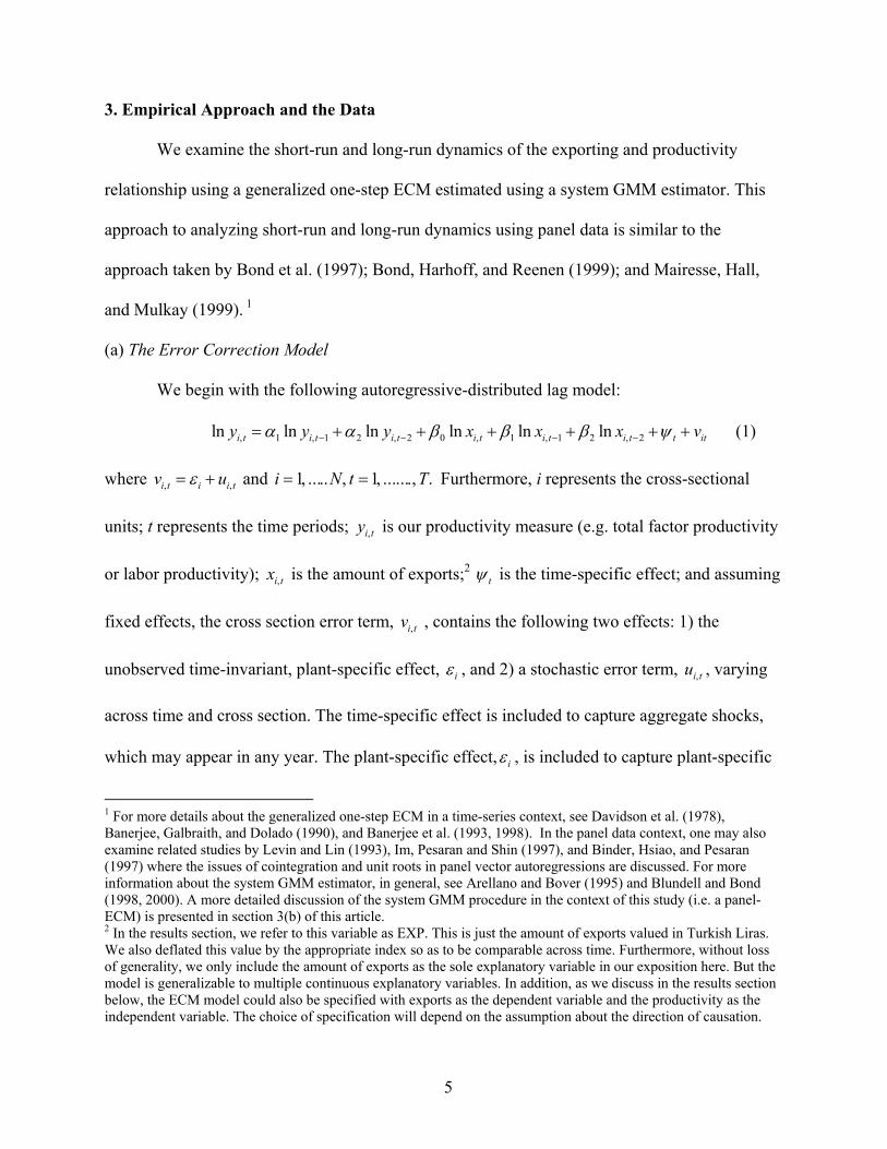
We begin with the following autoregressive-distributed lag model:

1 1 2 2 0 1 1 2 2ln ln ln ln ln lni t i t i t i t i t i t t ity y y x x x vα α β β β ψ, , − , − , , − , −= + + + + + + (1)

where i t i i tv uε, ,= + and 1 1i … N t …… T= , .. , = , ., . Furthermore, i represents the cross-sectional

units; t represents the time periods; i ty , is our productivity measure (e.g. total factor productivity

or labor productivity); i tx , is the amount of exports;2 tψ is the time-specific effect; and assuming

fixed effects, the cross section error term, i tv , , contains the following two effects: 1) the

unobserved time-invariant, plant-specific effect, iε , and 2) a stochastic error term, i tu , , varying

across time and cross section. The time-specific effect is included to capture aggregate shocks,

which may appear in any year. The plant-specific effect, iε , is included to capture plant-specific

1 For more details about the generalized one-step ECM in a time-series context, see Davidson et al. (1978), Banerjee, Galbraith, and Dolado (1990), and Banerjee et al. (1993, 1998). In the panel data context, one may also examine related studies by Levin and Lin (1993), Im, Pesaran and Shin (1997), and Binder, Hsiao, and Pesaran (1997) where the issues of cointegration and unit roots in panel vector autoregressions are discussed. For more information about the system GMM estimator, in general, see Arellano and Bover (1995) and Blundell and Bond (1998, 2000). A more detailed discussion of the system GMM procedure in the context of this study (i.e. a panel-ECM) is presented in section 3(b) of this article. 2 In the results section, we refer to this variable as EXP. This is just the amount of exports valued in Turkish Liras. We also deflated this value by the appropriate index so as to be comparable across time. Furthermore, without loss of generality, we only include the amount of exports as the sole explanatory variable in our exposition here. But the model is generalizable to multiple continuous explanatory variables. In addition, as we discuss in the results section below, the ECM model could also be specified with exports as the dependent variable and the productivity as the independent variable. The choice of specification will depend on the assumption about the direction of causation.

6

differences such as managerial ability, geographical location, and other unobserved factors. The

unobserved plant-specific effect, iε , is correlated with the explanatory variables, but not with the

changes in the explanatory variables.

The autoregressive-distributed lag model specification is appropriate if the short-run

relationship between exporting and productivity is the only object of interest. However, it does

not allow for a distinction between the long and short-run effects. We incorporate this distinction

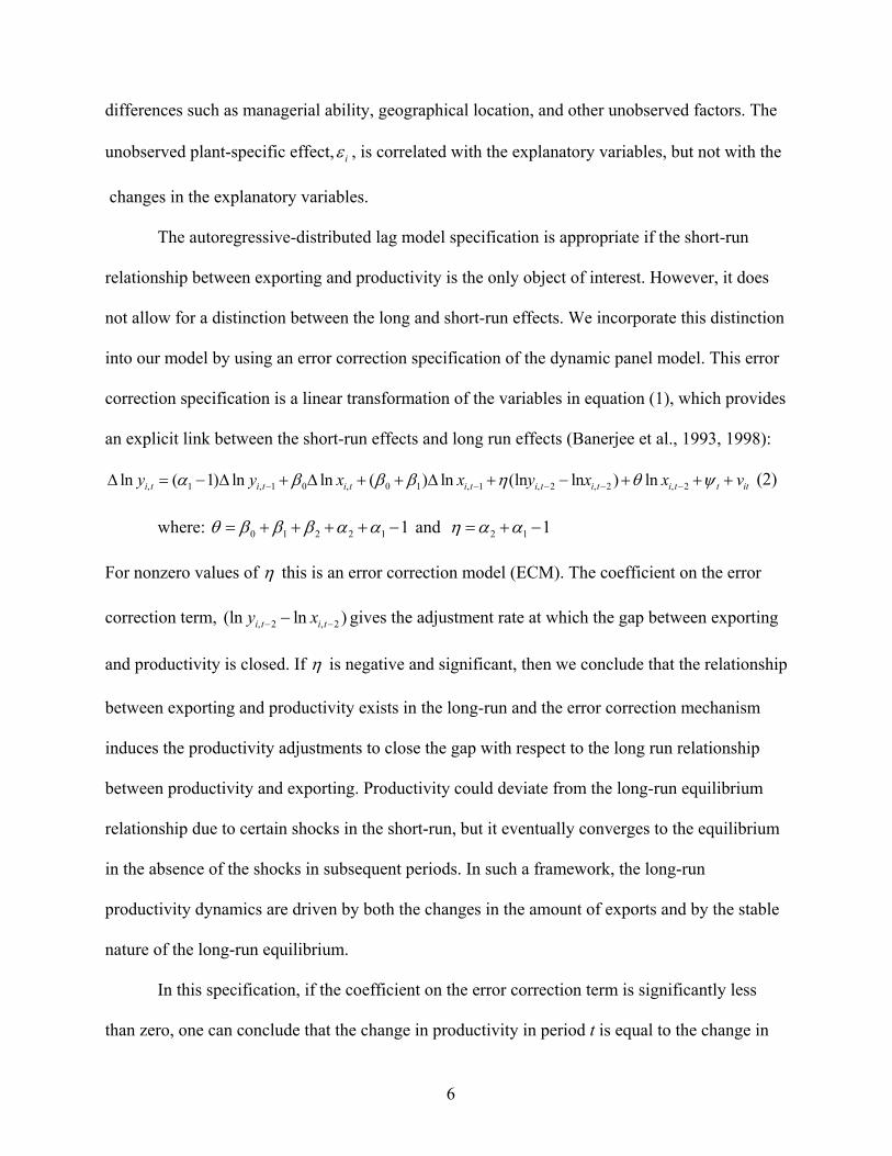
into our model by using an error correction specification of the dynamic panel model. This error

correction specification is a linear transformation of the variables in equation (1), which provides

an explicit link between the short-run effects and long run effects (Banerjee et al., 1993, 1998):

1 1 0 0 1 1 2 2 2ln ( 1) ln ln ( ) ln (ln ln ) lni t i t i t i t i t i t i t t ity y x x y x x vα β β β η θ ψ, , − , , − , − , − , −∆ = − ∆ + ∆ + + ∆ + − + + + (2)

where: 0 1 2 2 1 1θ β β β α α= + + + + − and 2 1 1η α α= + −

For nonzero values of η this is an error correction model (ECM). The coefficient on the error

correction term, 2 2(ln ln )i t i ty x, − , −− gives the adjustment rate at which the gap between exporting

and productivity is closed. If η is negative and significant, then we conclude that the relationship

between exporting and productivity exists in the long-run and the error correction mechanism

induces the productivity adjustments to close the gap with respect to the long run relationship

between productivity and exporting. Productivity could deviate from the long-run equilibrium

relationship due to certain shocks in the short-run, but it eventually converges to the equilibrium

in the absence of the shocks in subsequent periods. In such a framework, the long-run

productivity dynamics are driven by both the changes in the amount of exports and by the stable

nature of the long-run equilibrium.

In this specification, if the coefficient on the error correction term is significantly less

than zero, one can conclude that the change in productivity in period t is equal to the change in

7

the exports in period t and the correction for the change between productivity and its equilibrium

value in period t-1. If productivity is greater than its equilibrium level, it must decrease for the

model to approach equilibrium, and vice-versa. If the model is in equilibrium in period t-1, the

error correction term does not influence the change in exports in period t. In this case, the change

in the productivity in period t is equal to the change in the independent variable in period t. The

error-correcting model allows us to describe the adjustment of the deviation from the long-run

relationship between exporting and productivity. In this specification, the first three terms

(lagged growth rate of productivity, the contemporaneous and the one-period lagged growth of

exports) capture the short-run dynamics and the last two terms (error correction and the lagged

level of independent variable) provide a framework to test the long-run relationship between

productivity and exports.

In general, a long-run multiplier (φ ) is typically estimated separately and used to form

the error correction term 2 2(ln ln )i t i ty xφ, − , −− . With the use of 2 2(ln ln )i t i ty x, − , −− , the long-run

relationship is restricted to be homogeneous (Banerjee, Galbraith, and Dolado, 1990; Banerjee et

al., 1993). That is, the implied coefficient of φ = 1 indicates a proportional long-run relationship

between y and x. We also use the error correction term of the form 2 2(ln ln )i t i ty xφ, − , −− to avoid

this restrictive homogeneity assumption. Thus, in our formulation of the error correction model,

we can interpret the coefficient η directly as adjustments to disequilibrium although the true

equilibrium is given by 2 2(ln ln )i t i ty xφ, − , −− instead of 2 2(ln ln )i t i ty x, − , −− . Using this form of the

error correction term also allows us to calculate the true long-run relationship between exporting

and productivity, which can be written as, ˆ ˆ1 ( / ).θ η− The error correction specification of the

autoregressive distributed lag model that we used here then permits us to directly calculate and

analyze the short-run and long-run dynamics of the productivity and exporting relationship.

8

(b) The System GMM Estimation Procedure

For consistent and efficient parameter estimates of the panel data error correction model

specified in equation (2), we apply the system GMM approach proposed by Arellano and Bover

(1995) and Blundell and Bond (1998; 2000). This estimation procedure is especially appropriate

when: (i) N is large, but T is small; ii) the explanatory variables are endogenous; and iii)

unobserved plant-specific effects are correlated with other regressors. Under the assumptions that

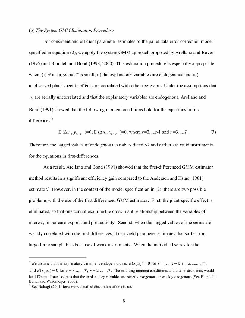
itu are serially uncorrelated and that the explanatory variables are endogenous, Arellano and

Bond (1991) showed that the following moment conditions hold for the equations in first

differences:3

, , , ,E ( )=0; E ( )=0; where =2,..., -1 and =3,..., .i t i t r i t i t ru y u x r t t T− −∆ ∆ (3)

Therefore, the lagged values of endogenous variables dated t-2 and earlier are valid instruments

for the equations in first-differences.

As a result, Arellano and Bond (1991) showed that the first-differenced GMM estimator

method results in a significant efficiency gain compared to the Anderson and Hsiao (1981)

estimator.4 However, in the context of the model specification in (2), there are two possible

problems with the use of the first differenced GMM estimator. First, the plant-specific effect is

eliminated, so that one cannot examine the cross-plant relationship between the variables of

interest, in our case exports and productivity. Second, when the lagged values of the series are

weakly correlated with the first-differences, it can yield parameter estimates that suffer from

large finite sample bias because of weak instruments. When the individual series for the

3 We assume that the explanatory variable is endogenous, i.e. ( ) 0 for 1,..., 1; 2,...... ,ir itE x u r t t T= = − = ;

and ( ) 0 for ,......, ; 2,......, .ir itE x u r s T s T≠ = = The resulting moment conditions, and thus instruments, would be different if one assumes that the explanatory variables are strictly exogenous or weakly exogenous (See Blundell, Bond, and Windmeijer, 2000). 4 See Baltagi (2001) for a more detailed discussion of this issue.

9

dependent and independent variable are highly persistent, and when T is small, the problem is

more severe.

Arellano and Bover (1995), however, noted that if the initial condition, 1iX , satisfies the

stationarity restriction 2( ) 0i iE X ε∆ = , then itX∆ will be correlated with iε if and only if 2iX∆ is

correlated with iε . The resulting assumption is that although there is a correlation between the

level of right-hand-side variables, itX , and the plant-specific effect, iε , no such correlation exists

between the differences of right-hand-side variables, itX∆ , and the plant-specific effect, iε . This

additional assumption gives rise to the level equation estimator, which exploits more moment

conditions. Lagged differences of explanatory variables, it rX −∆ , are used as additional

instruments for the equations in levels, when itX is mean stationary.

Blundell and Bond (1998) showed that the lagged differences of the dependent variable,

in addition to the lagged differences of the explanatory variables, are proper instruments for the

regression in the level equation as long as the initial conditions, 1iy , satisfy the stationary

restriction, 2( ) 0i iE Y ε∆ = . Thus, when both itX∆ and itY∆ are uncorrelated with iε , both lagged

differences of explanatory variables, it rX −∆ and lagged differences of dependent variable, it rY −∆ ,

are valid instruments for the equations in levels. Furthermore, Blundell and Bond (1998) show

that the moment conditions defined for the first-differenced equation can be combined with the

moment conditions defined for the level equation to estimate a system GMM. When the

explanatory variable is treated as endogenous, the GMM system estimator utilizes the following

moment conditions:

, , , ,( ) 0; ( ) 0; where 2,..., -1; and 3,...,i t i t r i t i t rE u y E u x r t t T− −∆ = ∆ = = = (4)

, , , ,( ) 0; ( ) 0; where 1; and 3,..., .i t i t r i t i t rE v y E v x r t T− −∆ = ∆ = = = (5)

10

This estimator combines the T-2 equations in differences with the T-2 equations in levels

into a single system. It uses the lagged levels of dependent and independent variables as

instruments for the difference equation and the lagged differences of dependent and independent

variables as instruments for the level equation. Blundell and Bond (1998) showed that this new

system GMM estimator results in consistent and efficient parameter estimates, and has better

asymptotic and finite sample properties.

We examined the nature of our data to determine whether the series for exporting and

productivity are persistent. Our estimates of the AR (1) coefficients on exporting and

productivity show that the series of exporting and productivity are highly persistent, thus the

lagged levels of exports and productivity provide weak instruments for the differences in the

first-differenced GMM model. As a result, we believe the system GMM estimator to be more

appropriate than the first-differenced estimator in the context of this study.

Thus, we combine the first-differenced version of the ECM with the level version of the

model, for which the instruments used must be orthogonal to the plant-specific effects. Note that

the level of the dependent productivity variable must be correlated with the plant-specific effects,

and we want to allow for the levels of the independent export variable to be potentially correlated

with the plant specific effect. This rules out using the levels of any variables as instruments for

the level equation. However, Blundell and Bond (1998) show that in autoregressive-distributed

lag models, first differences of the series can be uncorrelated with the plant specific effect

provided that the series have stationary means. In summary, the system GMM estimator uses

lagged levels of the productivity and exports variables as instruments for the first-difference

equation and lagged difference of the productivity and exports variables as instruments for the

level form of the model.

11

This system GMM estimator results in consistent and efficient parameter estimates, and

has good asymptotic and finite sample properties (relative to just straightforward estimation of

first-differences). Moreover, this estimation procedure allows us to examine the cross-sectional

relationship between the levels of exporting and productivity since the firm-specific effect is not

eliminated but rather controlled by the lagged differences of the dependent and independent

variables as instruments, assuming that the differences are not correlated with a plant-specific

effect, while levels are.

To determine whether our instruments are valid in the system GMM approach, we use the

specification tests proposed by Arellano and Bond (1991) and Arellano and Bover (1995). First,

we apply the Sargan test, a test of overidentifying restrictions, to determine any correlation

between instruments and errors. For an instrument to be valid, there should be no correlation

between the instrument and the error terms. The null hypothesis is that the instruments and the

error terms are independent. Thus, failure to reject the null hypothesis could provide evidence

that valid instruments are used. Second, we test whether there is a second order serial correlation

with the first differenced errors. The GMM estimator is consistent if there is no second order

serial correlation in the error term of the first-differenced equation. The null hypothesis in this

case is that the errors are serially uncorrelated. Thus, failure to reject the null hypothesis could

supply evidence that valid orthogonality conditions are used and the instruments are valid. One

would expect the differenced error term to be first order serially correlated, although the original

error term is not. Finally, we use the differenced Sargan test to determine whether the extra

instruments implemented in the level equations are valid. We compare the Sargan test statistic

for the first differenced estimator and the Sargan test statistic for the system estimator.

(c) The Data

12

This study uses unbalanced panel data on plants with more than 25 employees for the

T&A industry (ISIC 3212 and 3222), and MV&P industry (ISIC 3843) industries from 1987-

1997. Our sample represents a large fraction of the relevant population; textile(manufacture of

textile goods except wearing apparel, ISIC 3212) and apparel (manufacture of wearing apparel

except fur and leather, ISIC 3222) are subsectors of the textile, wearing apparel and leather

industry (ISIC 32), which accounts for 35 percent of the total manufacturing employment, nearly

23 percent of wages, 20 percent of the output produced in the total manufacturing industry and

approximately 48 percent of Turkish manufactured exports. The motor vehicles and parts

industry (ISIC 3843) accounts for 5 percent of the total manufacturing employment, nearly 6.6

percent of wages, 10 percent of the output produced in the total manufacturing industry, and

approximately 5.2 percent of Turkish manufactured exports. Thus, the data that is used in the

study accounts for 53.2 percent of the total Turkish merchandise exports.

The data was collected by the State Institute of Statistics in Turkey from the Annual

Surveys of Manufacturing Industries, and classified based on the International Standard

Industrial Classification (ISIC Rev.2). These plant-level data consist of output; capital, labor,

energy, and material inputs; investments; depreciation funds; import; export; and several plant

characteristics.5 These plant-level variables were also used to estimate the productivity indices

(i.e. total factor productivity (TFP) and labor productivity (LP)) using the Multilateral Index

approach of Good, Nadiri, and Sickles (1996).6

5 In the interest of space, a detailed description of how these variables are constructed is not presented here, but is available from the authors upon request. 6 We acknowledge that there may be conceptual difficulties in the use of this type of productivity measure in our analysis (as raised by Katayama, Lu, and Tybout (2003). However, all previous studies in the literature still use this type of productivity measure and a feasible/refined alternative estimation procedure for an appropriate productivity measure has not been put forward. A more detailed discussion of the approach used for calculating the plant-level TFPs can be seen in the Appendix.

13

An important issue to note here is that some of the export values in our data set were

missing for the years 1987, 1988, 1989 and 1997; even though the data for the other variables is

complete. Instead of dropping these years, we chose to augment the export data by using

interpolation and extrapolation techniques. To describe these techniques, consider a time series

with n time periods: 1x , 2x ,… nx . Interpolation fills in missing values for all observations with

missing data between non-missing observations. That is, if we have non-missing observations for

2x ,…, 8x and 11x ,…, 15x , then interpolation will produce estimates for 9x and 10x , but not for

1x . Extrapolation, on the other hand, fills in missing values both between and beyond non-

missing observations. Thus, if the series ran from 1x to 20x , then extrapolation will produce

estimates for 9x and 10x , but for 1x and 16x ,…, 20x as well. This approach for dealing with

missing data is not new and has been used in other studies (Efron, 1994; Little and Rubin, 1987;

Moore and Shelman, 2004; Rubin, 1976, 1987, 1996; Schafer, 1997; and Schenker et al., 2004).

It is important to emphasize here that this augmentation did not markedly change the relevant

results (i.e. signs, magnitude, and significance) of the estimated ECM model parameters using

only the non-missing data (1990-96).7

Our models are estimated using the plants that export continuously, plants that begin as

non-exporters during the first two years of the sample time period and become exporters

thereafter and stayed in the market continuously, and the plants that start as exporters and exit

during the last two years of the sample period. Plants that do not export at any point in the time

period and the plants that enter and exit the export market multiple times are excluded.

7 In the interest of space, the results for the non-augmented export data from 1990-96 are not reported here but are available from the authors upon request.

14

In general, the nature of our panel data is such that the cross-section component is large

but the time-series component is small. Hence, the system GMM estimation procedure above

would be appropriate in this case. Summary statistics of all the relevant variables are presented in

Table 1.

TABLE 1 ABOUT HERE

4. Results

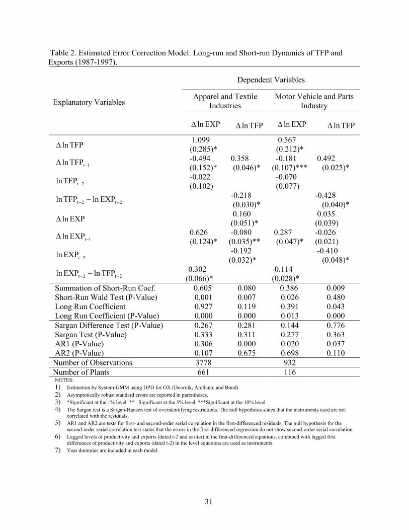
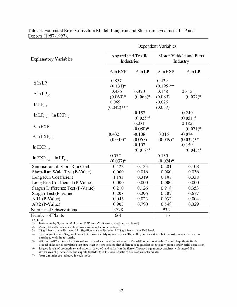
The estimated parameters of various ECMs are presented in Tables 2 and 3, respectively.

Specifically, Table 2 shows the estimated relationships between TFP growth and export growth,

while Table 3 shows the estimated relationships between LP growth and export growth. In these

estimated models, we used total factor productivity (TFP) and labor productivity (LP) as our

measures of productivity.

Note that in our discussion of equation (2) in the previous section, we assume that the

productivity measure is the dependent variable and amount of exports is one of the independent

variables. This implies that the direction of causation is from exports to productivity. Although

there are empirical studies that support the causal direction from exports to productivity (See, for

example, Kraay, 1997; Bigsten et al., 2002; Castellani, 2001), a number of empirical studies have

also shown that the direction of causation may be in the other direction (See Bernard and Jensen,

1999; Aw, Chung and Roberts, 1998; and Clerides, Lach, and Tybout, 1998). Hence, aside from

estimating the specification in equation (2), where the productivity measure is the dependent

variable, we also estimated ECM’s where the amount of exports is the dependent variable and

the productivity measure is the independent variable. In Tables 2 and 3, the first column for each

industry shows the effect of the productivity measure (i.e. either TFP or LP) on exporting, while

the second column for each industry shows the effect of exporting on the productivity measure.

TABLE 2 ABOUT HERE

15

TABLE 3 ABOUT HERE

As can be seen from these tables, the specification tests to check the validity of the

instruments are satisfactory. The test results show no evidence of second order serial correlation

in the first differenced residuals. Moreover, the validity of lagged levels dated t-2 and earlier as

instruments in the first-differenced equations, combined with lagged first differences dated t-2 as

instruments in the levels equations are not rejected by the Sargan test of overidentifying

restrictions.

The coefficients associated with the error correction terms in all the regression equations

are significant and negative as expected. Thus, the results show that there is a strong long-run

relationship between exporting and productivity. Furthermore, statistical significance of the error

correction terms also imply that, when there are deviations from long-run equilibrium, short-run

adjustments in the dependent variable will be made to re-establish the long-run equilibrium.

Now let us discuss each table in turn. In Table 2, for the equations where export growth is

the dependent variable, the error correction coefficients have statistically significant, negative

signs in both industries. However, the magnitude of the coefficients is different in each industry.

This means that the speed of the short-run adjustment is different for the two industries. For the

apparel and textile industries, the model converges quickly to equilibrium, with about 30 percent

of discrepancy corrected in each period (coefficient of -0.302). The speed of the adjustment from

the deviation in the long-run relationship between exports and productivity is slower in the

MV&P industry (-0.114) relative to the T&A industry. On the other hand, for the equation where

TFP growth is the dependent variable, the magnitudes of the error correction coefficients for the

MV&P industry is greater than the T&A industry (0.428 > 0.218). This means that the speed of

adjustment of TFP to temporary export shocks is slower in the T&A industry as compared to the

MV&P industry.

16

Another thing to note in Table 2 is the different short-run behaviors in the T&A versus

the MV&P industry. In the T&A industry, the speed of short-run export adjustment as a response

to temporary TFP shocks (-0.302) tend to be faster than the short-run TFP adjustments to

temporary export shocks (-0.218). In contrast, for the MV&P industry, the speed of short-run

export adjustment as a response to temporary TFP shocks (-0.114) tend to be slower than the

short-run TFP adjustments to temporary export shocks (-0.428). This suggests that short-run

industrial policy may need to be treated differently in both these industries due to the dissimilar

short-run dynamics.

The pattern of results in Table 3 is the same as the ones in Table 2. That is, the speed of

short-run export adjustments to LP shocks tend to be faster in the T&A industry (-0.377) as

compared to the MV&P industry (-0.135). In contrast, the speed of adjustment of LP to

temporary export shocks is slower in the T&A industry (-0.157) as compared to the MV&P

industry (-0.240). Also, the speed of short-run export adjustment as a response to temporary LP

shocks (-0.377) tend to be faster than the short-run LP adjustments to temporary export shocks (-

0.157). Conversely, for the MV&P industry, the speed of short-run export adjustment as a

response to temporary LP shocks (-0.135) tend to be slower than the short-run TFP adjustments

to temporary export shocks (-0.24). These results again suggest that the potential industry-

specific short-run impacts should be taken into account setting temporary industrial policy.

The coefficient of the error correction term gives us an indication of the speed of

adjustment, but it is also important to examine the magnitudes of the short-run effects as

measured by the short-run coefficient. From equation (2), the short-run coefficient is computed

by adding the coefficients of the contemporaneous and lagged dependent variable. From Tables 2

and 3, it is evident that the magnitude of the short-run export response to a temporary

productivity shock is greater than the short-run productivity effect of a temporary export shock

17

(in both industries). This suggests that temporary shocks in productivity will result in bigger

short-run export adjustments relative to the converse.

Aside from short-run adjustments of the variables, it is also important to examine the

long-run relationships implied from the ECMs. For this we use the long-run elasticities of the

dependent variables to the independent variables (See Tables 2 and 3). These long-run elasticities

are calculated by subtracting the ratio of the coefficient of the scale effect (lag value of

independent variable) to the coefficient of the error correction term from one. The statistical

significance of these elasticities is tested with a Wald test. The test results indicate that the

estimated long-run elasticities for all the estimated equations are statistically significant (at the

5% level) in both industries.

In Table 2, for the equations where export growth is the dependent variable, the long-run

elasticities indicate that long-run export response to permanent shocks in TFP is large (for both

industries). On the other hand, for the case where TFP is the dependent variable, the long-run

elasticities suggest that long-run TFP adjustments to permanent changes in exports are lower.

The results are very similar for the case of LP (Table 3). The long-run elasticities reveal that

long-run export response to permanent shocks in LP is tend to be greater than the LP response to

permanent changes in exports (for both industries).

Overall, the results from the long-run elasticities show that productivity response to

permanent shocks in exports is lower than the export response to the permanent shocks in

productivity for both the T&A and MV&P industries. Moreover, our analysis of short-run

dynamics reveals that, for the MV&P industry, short-run productivity adjustments to temporary

shocks in exports tend be faster than the short-run export adjustments to temporary shocks in

productivity. For the apparel industry, short-run export adjustments due to temporary

productivity shocks are faster relative to the short-run productivity adjustments from temporary

18

export shocks. However, the estimated short-run coefficient in both industries indicates that

short-run productivity response to temporary export shocks is larger that the short-term export

response to temporary productivity shocks. These results suggest similar behaviors in terms of

the magnitudes of the short-run and long-run effects of exports/productivity shocks. But speed of

short-run adjustments tends to be different depending on the type of industry. Knowledge of

these plant behaviors can help improve the design of industrial policies that would allow further

economic growth in Turkey.

5. Conclusions and Policy Implications In this paper, we examine the short-run and the long-run dynamics of the relationship

between export levels and productivity for two Turkish manufacturing industries. An error

correction model is estimated using a system GMM estimator to overcome problems associated

with unobserved plant-specific effects, persistence, and endogeneity. This approach allows us to

obtain consistent and efficient estimates of the short-run and long-run relationships of exports

and productivity. From these estimates, we conclude that permanent productivity shocks induce

larger long-run export level responses, as compared to the effect of permanent export shocks on

long-run productivity. A similar behavior is evident with respect to the magnitude of the effects

of temporary shocks on short-run behavior. In addition, for the T&A industry, our short-run

analysis shows that temporary export shocks usually result in faster short-run productivity

adjustments, as compared to the effects of productivity shocks on short-run exports. The

converse is true for the MV&P industry.

From an industrial policy perspective, our analysis suggests that policies which induce

permanent productivity enhancements would result in large long-run export effects. Hence,

policies aimed at permanently improving productivity should be implemented by the policy

makers to obtain sustainable export performance and a bigger role in the global market. This may

19

then lead to more sustained economic growth. This insight may help explain the apparent failure

of the trade liberalization policies in the 1980s to sustain productivity and growth in the

economy. Most developing countries enact policies to promote exports on the assumption that it

will be good for productivity and economic growth. From our results, there would be a positive

productivity response if this was a permanent promotion policy, but this kind of policy would

still only generate a small long-term effect on productivity and/or economic growth.

In addition, if the export promotion policy is temporary, there would probably be

differential short-run speed of adjustments depending on the type of industry where it is

implemented. For the MV&P industry, our results suggest that a temporary export promotion

policy would result in a fast productivity response. But in the T&A industry, a temporary export

promotion policy may lead to a slower productivity response. The reason is that the MV&P

industry in Turkey tends to be large plants that are heavily invested in technology, while plants

in the apparel industry tend to be small to medium sized with fewer investments in technology.

Hence, if government policy makers want to implement short-run policies to show fast

performance effects, then they must consider the short-run dynamic behavior of plants in

different industries in their decision-making. On the other hand, in both the T&A and MV&P

industry, there would be larger short-run export adjustments from temporary shocks in

productivity relative to the short-run productivity enhancements from temporary export shocks.

This is consistent with our long-run insights that productivity enhancements tend to have larger

export effects, which again point to the appropriateness of enacting productivity-enhancing

policies as the main tool for driving export and economic growth.

20

Acknowledgements

We are greatly indebted to Omer Gebizlioglu, Ilhami Mintemur and Emine Kocberber at State Institute of Statistics in Turkey for allowing us to have an access to the data for this study. We also thank discussants and participants at the 11th International Conference on Panel Data, 2004 North American Summer Meeting of the Econometric Society, 2004 International Industrial Organization Conference for their suggestions that helped us greatly in revising the paper.

21

Appendix A: Calculation of Plant-level Total Factor Productivity

The main measure of productivity used in this study is total factor productivity (TFP). In

the plant-level analysis, we construct a multilateral index to measure the plant-level TFP for the

period 1987-1997. In this study, we use Good, Nadiri, and Sickles’s (1996) approach for

computing the multilateral TFP index. In their approach, different hypothetical plant reference

points are constructed for each cross-section, and then the hypothetical plants are linked together

over time. This type of multilateral index has the advantage of providing measures either from

year to year or from a sequence of years, through the process of chain-linking.

In this study, the multilateral TFP index measure for plant j, which produces a single

output jtY using inputs ijtX with cost shares ijtS , is calculated as follows:

( ) ( )12ln ln ln ln lnt

kjt jt t kkTFP Y Y Y Y −

== − + − −∑

( )( ) ( )( )1 1

112 21 2 1ln ln ln lnn t n

it ik ikijt it ijt ik iki k iS S X X S S X X −−= = =

+ − + + − ∑ ∑ ∑ (A.1)

where ln tY and ln itX are the natural log of the geometric mean of output and the natural log of

the geometric mean of the inputs (capital, energy, labor, and material inputs) across all plants in

time t, respectively. The subscript j represents individual plants such that j = 1, 2, …, N. The

subscript i is used to represent the different inputs where i = 1, 2, …, n. The subscript k

represents time period from k = 2, 3, …, t (i.e. if we are considering 10 years in the analysis, k =

2, 3, …, 10).

The first two terms in the first line measure the plant’s output relative to the hypothetical

plant in the base year. The first term describes the deviation between the output of plant j and the

representative plant’s output, ln tY , in year t. This first sum allows us to make comparisons

between cross-sections. The second term sums the change in the hypothetical plant’s output

22

across all years, while chaining the hypothetical plant values back to the base year. This allows

us to measure the change in output of a typical plant over years. The following terms provide

similar information. However, it is for inputs using cost shares and arithmetic average cost shares

in each year as weights. Cost shares are just the proportion of the cost of input i relative to the

total cost of all inputs. The resulting measure is the total factor productivity of plant j in year t

relative to the hypothetical plant in the base year (1987, in this case). With this measure the

distribution of plant-level total factor productivity can then be analyzed.

Aside from the plant-level TFP, we also calculate the plant-level labor productivity using

the same multilateral index calculation described above but only using labor on the input side of

the calculation. Using the labor productivity in our analysis ensures that our analysis is robust to

any changes in productivity measure used. However, it is important to note that labor

productivity is only a partial measure of TFP and has its own shortcomings. For example, if the

production technology among plants within the industry differs such that they do not have

similar input-output ratios, then labor productivity is not a good measure of efficiency and may

be a misleading measure of performance. The TFP may be more appropriate in this case.

Nevertheless, using the labor productivity would allow us to somehow assess the robustness of

our results.

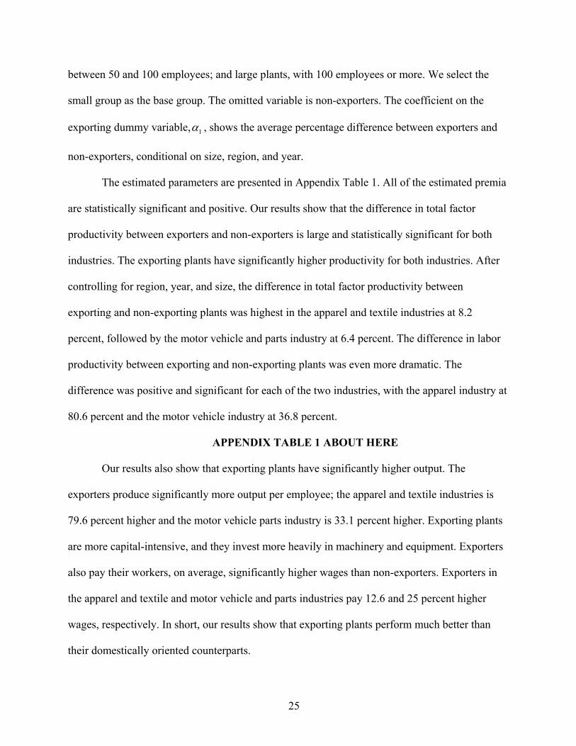
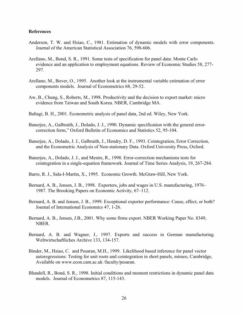
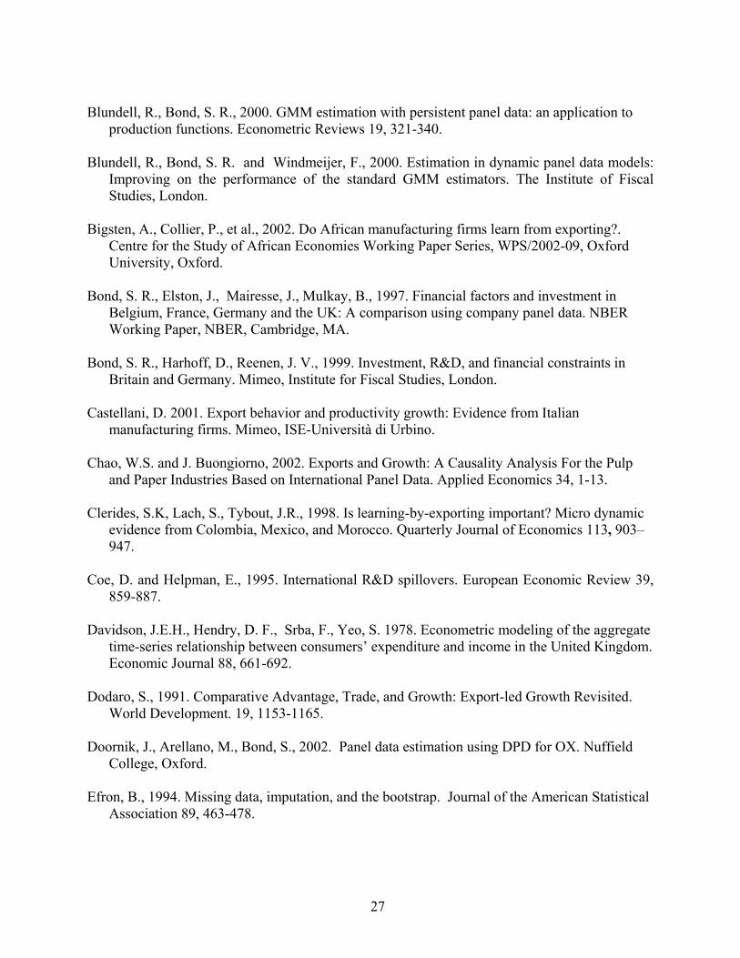
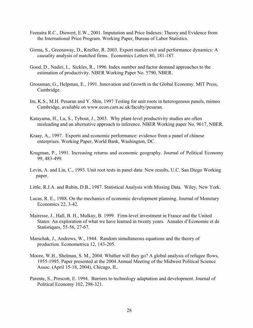
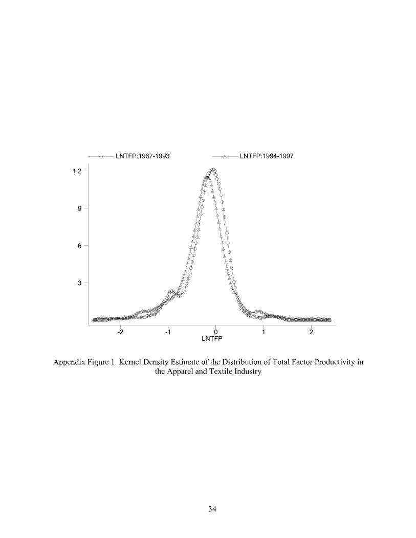
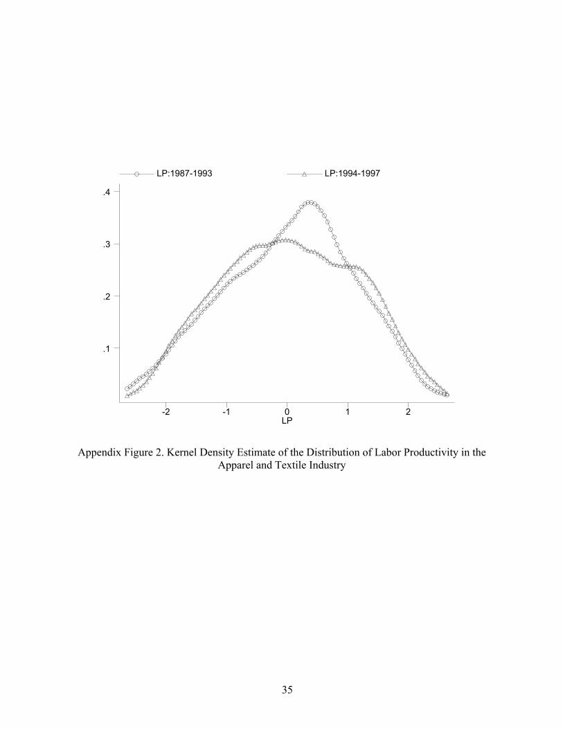
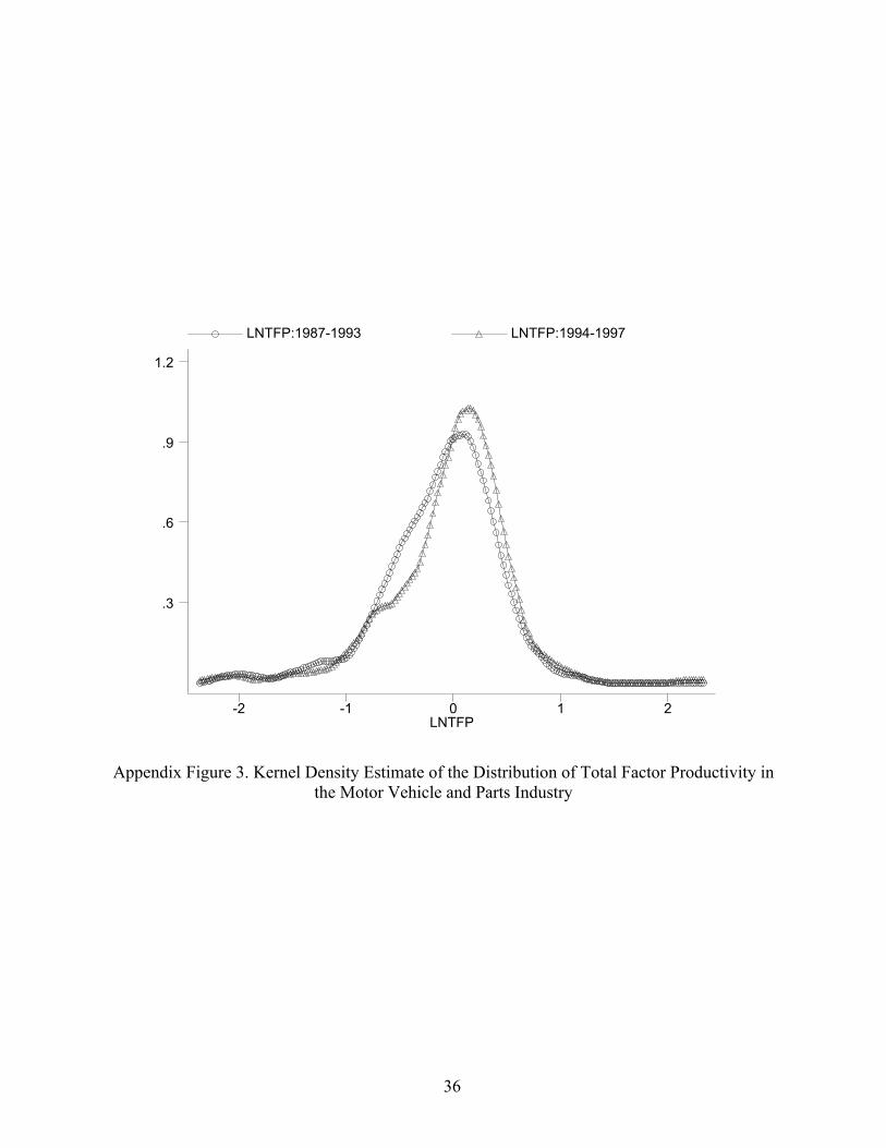
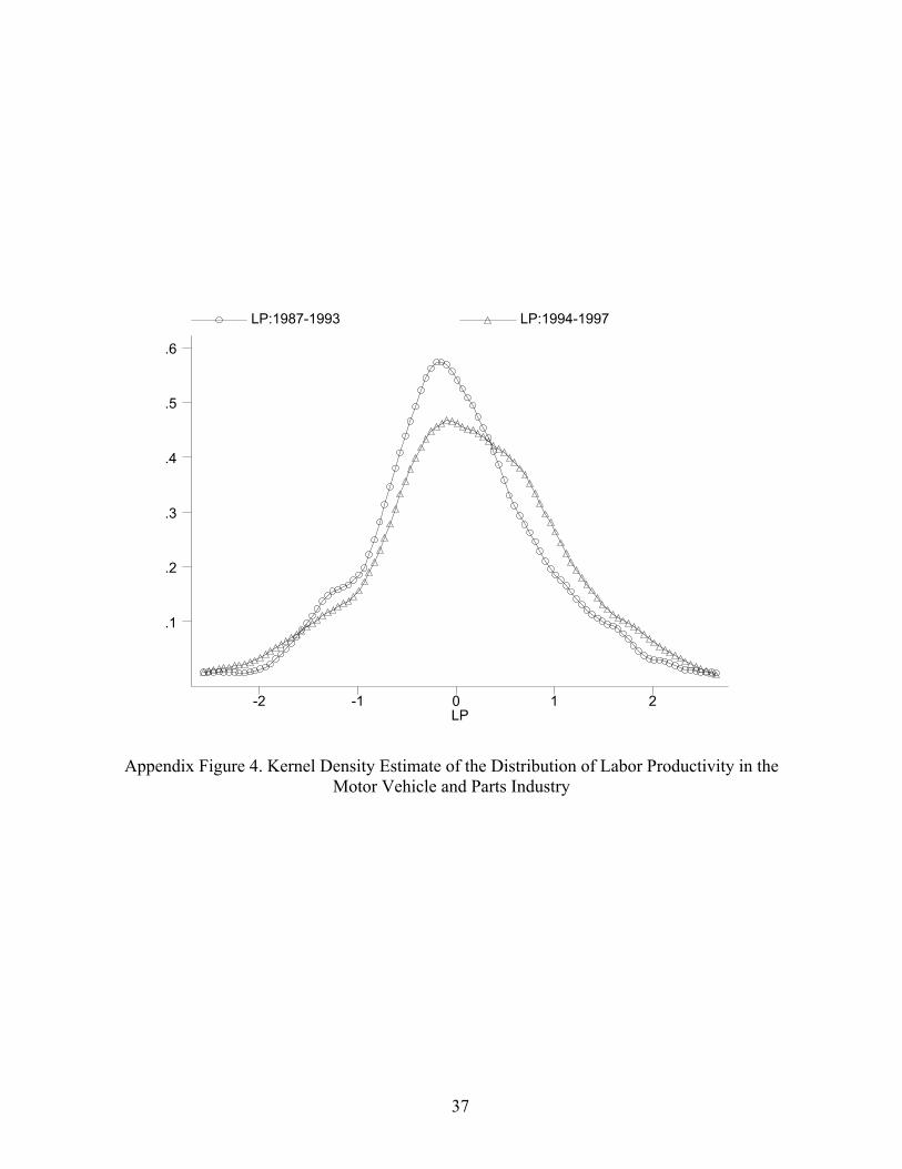
We use kernel density estimates for the plant-level TFP and labor productivity measure to

summarize the distribution of plant productivity. Appendix Figures 1-4 show kernel density

estimates of TFP and labor productivity for the industries, respectively. The kernel density was

estimated for two time periods, from 1987-1993 and 1994-1997. These two time periods were

chosen because the country suffered an economic crisis in 1994 and soon afterwards the

government introduced institutional changes in their economic and financial policies. For

23

example, the Economic Stabilization and Structural Adjustment Program was enacted, where

export-oriented policies such as subsidies and wage suppression were put in place. The foreign

exchange system was regulated and the capital inflow was controlled during this period. Prior to

1994, the pre-dominant policies of the government were the opposite of the post-1994 period

(i.e. the government relinquished control of capital markets, eliminate subsidies, and increase

wages). Hence, the period 1987-93 can be called the pre-crisis period and the period 1994-1997

is the post-crisis period.

APPENDIX FIGURE 1 ABOUT HERE

APPENDIX FIGURE 2 ABOUT HERE

Appendix Figures 3-4 clearly show that there is a slight rightward shift in TFP and labor

productivity during the post-crisis period in Motor vehicle and Parts industry. For the Apparel

and Textile industry there is a rightward shift in the labor productivity but not in the TFP.

APPENDIX FIGURE 3 ABOUT HERE

APPENDIX FIGURE 4 ABOUT HERE

24

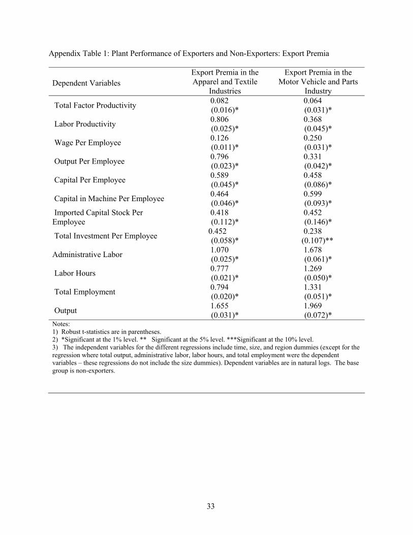
Appendix B: Plant Performance of Exporters and Non-exporters: Export Premia

This section reports estimates of the proportional differences between the characteristics

of exporting and non-exporting plants in the Turkish apparel and textile and motor vehicle and

parts industries by forming the following regression (See Bernard and Wagner, 1997):

X 0 1 2 3 4it it it it t itExporter Size Region Year eα α α α α= + + + + + , (A.2)

where X stands for either the log or the share of plant characteristics that reflect plant capabilities

in productivity, technology, and employment.8 Exporter is a dummy variable for the export

status, taking a value of 1 if the plant exports in the current year. Year dummies are included to

capture macroeconomic shocks and the changes in the institutional environment. The

agglomeration effect might be important in explaining the differences in plant characteristics (see

Krugman, 1991 and Porter, 1998). There are large development disparities across Turkey’s

regions because of different regional capabilities such as infrastructure, rule of law, quality of

public services, localized spillovers, the export and import density, foreign investment intensity

(to take advantage of international spillovers, (See Coe and Helpman,1995). Therefore, we

included regional dummies to correct for the exogenous disparities in the productivity

differences across the regions. Finally, the plant size is included to capture differences in the

production technology across plants of different sizes. One would expect the larger plants to be

more productive for two reasons. They benefit from scale economies and have access to more

productive technology to a greater extent. However, they tend to be less flexible in their

operation which affects productivity negatively. In order to capture the size effects, we divide the

plants into three size groups: small plants, with less than 50 employees; medium plants, with

8 We also included the export intensity (the ratio of exports to output of the plant) as an explanatory variable in the regression; however, the results did not change. The export premia was greater for the plants that export a higher proportion of their output.

25

between 50 and 100 employees; and large plants, with 100 employees or more. We select the

small group as the base group. The omitted variable is non-exporters. The coefficient on the

exporting dummy variable, 1α , shows the average percentage difference between exporters and

non-exporters, conditional on size, region, and year.

The estimated parameters are presented in Appendix Table 1. All of the estimated premia

are statistically significant and positive. Our results show that the difference in total factor

productivity between exporters and non-exporters is large and statistically significant for both

industries. The exporting plants have significantly higher productivity for both industries. After

controlling for region, year, and size, the difference in total factor productivity between

exporting and non-exporting plants was highest in the apparel and textile industries at 8.2

percent, followed by the motor vehicle and parts industry at 6.4 percent. The difference in labor

productivity between exporting and non-exporting plants was even more dramatic. The

difference was positive and significant for each of the two industries, with the apparel industry at

80.6 percent and the motor vehicle industry at 36.8 percent.

APPENDIX TABLE 1 ABOUT HERE

Our results also show that exporting plants have significantly higher output. The

exporters produce significantly more output per employee; the apparel and textile industries is

79.6 percent higher and the motor vehicle parts industry is 33.1 percent higher. Exporting plants

are more capital-intensive, and they invest more heavily in machinery and equipment. Exporters

also pay their workers, on average, significantly higher wages than non-exporters. Exporters in

the apparel and textile and motor vehicle and parts industries pay 12.6 and 25 percent higher

wages, respectively. In short, our results show that exporting plants perform much better than

their domestically oriented counterparts.

26

References

Anderson, T. W. and Hsiao, C., 1981. Estimation of dynamic models with error components. Journal of the American Statistical Association 76, 598-606.

Arellano, M., Bond, S. R., 1991. Some tests of specification for panel data: Monte Carlo

evidence and an application to employment equations. Review of Economic Studies 58, 277-297.

Arellano, M., Bover, O., 1995. Another look at the instrumental variable estimation of error

components models. Journal of Econometrics 68, 29-52. Aw, B., Chung, S., Roberts, M., 1998. Productivity and the decision to export market: micro

evidence from Taiwan and South Korea. NBER, Cambridge MA. Baltagi, B. H., 2001. Econometric analysis of panel data, 2nd ed. Wiley, New York. Banerjee, A., Galbraith, J., Dolado, J. J., 1990. Dynamic specification with the general error-

correction form,” Oxford Bulletin of Economics and Statistics 52, 95-104. Banerjee, A., Dolado, J. J., Galbraith, J., Hendry, D. F., 1993. Cointegration, Error Correction,

and the Econometric Analysis of Non-stationary Data. Oxford University Press, Oxford. Banerjee, A., Dolado, J. J., and Mestre, R., 1998. Error-correction mechanisms tests for

cointegration in a single-equation framework. Journal of Time Series Analysis, 19, 267-284. Barro, R. J., Sala-I-Martin, X., 1995. Economic Growth. McGraw-Hill, New York. Bernard, A. B., Jensen, J. B., 1998. Exporters, jobs and wages in U.S. manufacturing, 1976–

1987. The Brooking Papers on Economic Activity, 67–112. Bernard, A. B. and Jensen, J. B., 1999. Exceptional exporter performance: Cause, effect, or both?

Journal of International Economics 47, 1-26. Bernard, A. B., Jensen, J.B., 2001. Why some firms export. NBER Working Paper No. 8349,

NBER. Bernard, A. B. and Wagner, J., 1997. Exports and success in German manufacturing.

Weltwirtschaftliches Archive 133, 134-157. Binder, M., Hsiao, C. and Pesaran, M.H., 1999. Likelihood based inference for panel vector

autoregressions: Testing for unit roots and cointegration in short panels, mimeo, Cambridge, Available on www.econ.cam.ac.uk /faculty/pesaran.

Blundell, R., Bond, S. R., 1998. Initial conditions and moment restrictions in dynamic panel data

models. Journal of Econometrics 87, 115-143.

27

Blundell, R., Bond, S. R., 2000. GMM estimation with persistent panel data: an application to

production functions. Econometric Reviews 19, 321-340. Blundell, R., Bond, S. R. and Windmeijer, F., 2000. Estimation in dynamic panel data models:

Improving on the performance of the standard GMM estimators. The Institute of Fiscal Studies, London.

Bigsten, A., Collier, P., et al., 2002. Do African manufacturing firms learn from exporting?.

Centre for the Study of African Economies Working Paper Series, WPS/2002-09, Oxford University, Oxford.

Bond, S. R., Elston, J., Mairesse, J., Mulkay, B., 1997. Financial factors and investment in

Belgium, France, Germany and the UK: A comparison using company panel data. NBER Working Paper, NBER, Cambridge, MA.

Bond, S. R., Harhoff, D., Reenen, J. V., 1999. Investment, R&D, and financial constraints in

Britain and Germany. Mimeo, Institute for Fiscal Studies, London. Castellani, D. 2001. Export behavior and productivity growth: Evidence from Italian

manufacturing firms. Mimeo, ISE-Università di Urbino. Chao, W.S. and J. Buongiorno, 2002. Exports and Growth: A Causality Analysis For the Pulp

and Paper Industries Based on International Panel Data. Applied Economics 34, 1-13. Clerides, S.K, Lach, S., Tybout, J.R., 1998. Is learning-by-exporting important? Micro dynamic

evidence from Colombia, Mexico, and Morocco. Quarterly Journal of Economics 113, 903–947.

Coe, D. and Helpman, E., 1995. International R&D spillovers. European Economic Review 39,

859-887. Davidson, J.E.H., Hendry, D. F., Srba, F., Yeo, S. 1978. Econometric modeling of the aggregate

time-series relationship between consumers’ expenditure and income in the United Kingdom. Economic Journal 88, 661-692.

Dodaro, S., 1991. Comparative Advantage, Trade, and Growth: Export-led Growth Revisited.

World Development. 19, 1153-1165. Doornik, J., Arellano, M., Bond, S., 2002. Panel data estimation using DPD for OX. Nuffield

College, Oxford. Efron, B., 1994. Missing data, imputation, and the bootstrap. Journal of the American Statistical

Association 89, 463-478.

28

Feenstra R.C., Diewert, E.W., 2001. Imputation and Price Indexes: Theory and Evidence from the International Price Program. Working Paper, Bureau of Labor Statistics.

Girma, S., Greenaway, D., Kneller, R. 2003. Export market exit and performance dynamics: A

causality analysis of matched firms. Economics Letters 80, 181-187. Good, D., Nadiri, I., Sickles, R., 1996. Index number and factor demand approaches to the

estimation of productivity. NBER Working Paper No. 5790, NBER. Grossman, G., Helpman, E., 1991. Innovation and Growth in the Global Economy. MIT Press,

Cambridge. Im, K.S., M.H. Pesaran and Y. Shin, 1997 Testing for unit roots in heterogenous panels, mimeo Cambridge, available on www.econ.cam.ac.uk/faculty/pesaran. Katayama, H., Lu, S., Tybout, J., 2003. Why plant-level productivity studies are often

misleading and an alternative approach to inference. NBER Working paper No. 9617, NBER. Kraay, A., 1997. Exports and economic performance: evidence from a panel of chinese

enterprises. Working Paper, World Bank, Washington, DC. Krugman, P., 1991. Increasing returns and economic geography. Journal of Political Economy

99, 483-499. Levin, A. and Lin, C., 1993. Unit root tests in panel data: New results, U.C. San Diego Working paper. Little, R.J.A. and Rubin, D.B., 1987. Statistical Analysis with Missing Data. Wiley, New York. Lucas, R. E., 1988. On the mechanics of economic development planning. Journal of Monetary

Economics 22, 3-42. Mairesse, J., Hall, B. H., Mulkay, B. 1999. Firm-level investment in France and the United

States: An exploration of what we have learned in twenty years. Annales d’Economie et de Statistiques, 55-56, 27-67.

Marschak, J., Andrews, W., 1944. Random simultaneous equations and the theory of

production. Econometrica 12, 143-205. Moore, W.H., Shelman, S. M., 2004. Whither will they go? A global analysis of refugee flows,

1955-1995. Paper presented at the 2004 Annual Meeting of the Midwest Political Science Assoc. (April 15-18, 2004), Chicago, IL.

Parente, S., Prescott, E. 1994. Barriers to technology adaptation and development. Journal of

Political Economy 102, 298-321.

29

Porter, M. E., 1998. Clusters and new economies of competition. Harvard Business Review Nov-Dec, 77-90.

Pugel T., 2004. International Economics. 12th ed., McGraw Hill, New York. Rivera-Batiz, L. A., Romer, P. 1991. Economic integration and endogenous growth. Quarterly

Journal of Economics. 106, 531-555. Roberts, M. Tybout, J.R., 1997. The decision to export in Colombia: An empirical model of

entry with sunk costs. American Economic Review 87, 545-564. Rubin, D.B., 1976. Inference and missing data. Biometrika 63, 581–592. Rubin, D.B., 1987. Multiple Imputation for Nonresponse in Surveys. Wiley, NY. Rubin, D.B., 1996. Multiple imputation after 18+ years. Journal of the American Statistical

Association 91, 473-489. Schafer, J.L., 1997. Analysis of Incomplete Multivariate Data. Chapman and Hall, New York. Schenker, N., Raghunathan, T., et al., 2004. Multiple imputation of family income and personal

earnings in the National Helath Interview Survey: Methods and examples. Technical Document, National Center for Health Statistics, Center for Disease Control (CDC), Atlanta.

Wagner, J., 2002. The causal effects of exports on firm size and labor productivity: first evidence

from a matching approach. Economics Letters 77, 287-292. Yasar, M., and C.J. Morrison Paul, 2004. Technology transfer and productivity at the plant

level. Unpublished Manuscript. Emory University

30

Table 1. Descriptive statistics from 1987-1997 (Y, K, E, and M are in Constant Value Quantities at 1987 Prices, in ‘000 Turkish Liras; L is in total hours worked in production per year)

Statistics A. Apparel and Textile Industries Mean Standard Deviation Minimum Maximum Output (Y) 1,951.53 4,386.20 3.09 115,994.70Material (M) 1,690.16 3,428.79 0.02 90,651.77Labor (L) 172.39 321.15 0.01 7,960.79Energy (E) 48.85 316.51 0.02 13,469.06Capital (K) 1,327.99 12,395.41 0.136 500,876.40 Small 0.585 Medium 0.203 Large 0.212 TFP Growth (∆lnTFP) 0.011 LP Growth (∆lnLP) 0.032 Export Growth (∆lnEXP)

0.081

Number of Observations 7453 Number of Plants 1265

Statistics B. MV&P Industry Mean Standard Deviation Minimum Maximum

Output (Y) 12,303.93 59,821.87 23.93 1,212,264.13Material (M) 8,269.86 41,860.24 0.41 793,683.63Labor (L) 336.62 933.14 0.01 18,141.64Energy (E) 237.28 1,023.14 0.13 22,178.53Capital (K) 5,506.36 31,480.68 0.60 720,275.88 Small* 0.514 Medium 0.173 Large 0.313 TFP Growth (∆lnTFP) 0.060 LP Growth (∆lnLP) 0.056 Export Growth (∆lnEXP)

0.165

Number of Observations 2211 Number of Plants 328 *We divide the plants into three size groups: small plants, with less than 50 employees; medium plants, between 50 and 100 employees; and large plants, with 100 employees or more.

31

Table 2. Estimated Error Correction Model: Long-run and Short-run Dynamics of TFP and Exports (1987-1997).

Dependent Variables

Apparel and Textile Industries

Motor Vehicle and Parts Industry Explanatory Variables

EXPln∆ TFPln∆ EXPln∆ TFPln∆

TFPln∆ 1.099 (0.285)* 0.567

(0.212)*

1tTFPln −∆ -0.494 (0.152)*

0.358 (0.046)*

-0.181 (0.107)***

0.492 (0.025)*

2tTFPln − -0.022 (0.102) -0.070

(0.077)

2t2t EXPlnTFPln −− − -0.218 (0.030)* -0.428

(0.040)*

EXPln∆ 0.160 (0.051)* 0.035

(0.039) 1tEXPln −∆ 0.626

(0.124)* -0.080 (0.035)**

0.287 (0.047)*

-0.026 (0.021)

2tEXPln − -0.192 (0.032)* -0.410

(0.048)* 2t2t TFPlnEXPln −− − -0.302

(0.066)* -0.114 (0.028)*

Summation of Short-Run Coef. 0.605 0.080 0.386 0.009 Short-Run Wald Test (P-Value) 0.001 0.007 0.026 0.480 Long Run Coefficient 0.927 0.119 0.391 0.043 Long Run Coefficient (P-Value) 0.000 0.000 0.013 0.000 Sargan Difference Test (P-Value) 0.267 0.281 0.144 0.776 Sargan Test (P-Value) 0.333 0.311 0.277 0.363 AR1 (P-Value) 0.306 0.000 0.020 0.037 AR2 (P-Value) 0.107 0.675 0.698 0.110 Number of Observations 3778 932 Number of Plants 661 116 NOTES: 1) Estimation by System-GMM using DPD for OX (Doornik, Arellano, and Bond) 2) Asymptotically robust standard errors are reported in parentheses. 3) *Significant at the 1% level. ** Significant at the 5% level. ***Significant at the 10% level. 4) The Sargan test is a Sargan-Hansen test of overidentifying restrictions. The null hypothesis states that the instruments used are not

correlated with the residuals. 5) AR1 and AR2 are tests for first- and second-order serial correlation in the first-differenced residuals. The null hypothesis for the

second-order serial correlation test states that the errors in the first-differenced regression do not show second-order serial correlation. 6) Lagged levels of productivity and exports (dated t-2 and earlier) in the first-differenced equations, combined with lagged first

differences of productivity and exports (dated t-2) in the level equations are used as instruments. 7) Year dummies are included in each model.

32

Table 3. Estimated Error Correction Model: Long-run and Short-run Dynamics of LP and Exports (1987-1997).

Dependent Variables

Apparel and Textile Industries

Motor Vehicle and Parts Industry Explanatory Variables

EXPln∆ LPln∆ EXPln∆ LPln∆

LPln∆ 0.857 (0.131)* 0.429

(0.195)**

1tLPln −∆ -0.435 (0.060)*

0.320 (0.068)*

-0.148 (0.089)

0.345 (0.037)*

2tLPln − 0.069 (0.042)*** -0.026

(0.057)

2t2t EXPlnLPln −− − -0.157 (0.025)* -0.240

(0.051)*

EXPln∆ 0.231 (0.080)* 0.182

(0.071)* 1tEXPln −∆ 0.432

(0.045)* -0.108 (0.067)

0.316 (0.049)*

-0.074 (0.037)**

2tEXPln − -0.107 (0.017)* -0.159

(0.045)* 2t2t LPlnEXPln −− − -0.377

(0.037)* -0.135 (0.024)*

Summation of Short-Run Coef. 0.422 0.123 0.281 0.108 Short-Run Wald Test (P-Value) 0.000 0.016 0.080 0.036 Long Run Coefficient 1.183 0.319 0.807 0.338 Long Run Coefficient (P-Value) 0.000 0.000 0.000 0.000 Sargan Difference Test (P-Value) 0.210 0.126 0.918 0.353 Sargan Test (P-Value) 0.208 0.296 0.707 0.677 AR1 (P-Value) 0.046 0.023 0.032 0.004 AR2 (P-Value) 0.905 0.790 0.548 0.329 Number of Observations 3778 932 Number of Plants 661 116 NOTES: 1) Estimation by System-GMM using DPD for OX (Doornik, Arellano, and Bond) 2) Asymptotically robust standard errors are reported in parentheses. 3) *Significant at the 1% level. ** Significant at the 5% level. ***Significant at the 10% level. 4) The Sargan test is a Sargan-Hansen test of overidentifying restrictions. The null hypothesis states that the instruments used are not

correlated with the residuals. 5) AR1 and AR2 are tests for first- and second-order serial correlation in the first-differenced residuals. The null hypothesis for the

second-order serial correlation test states that the errors in the first-differenced regression do not show second-order serial correlation. 6) Lagged levels of productivity and exports (dated t-2 and earlier) in the first-differenced equations, combined with lagged first

differences of productivity and exports (dated t-2) in the level equations are used as instruments. 7) Year dummies are included in each model.

33

Appendix Table 1: Plant Performance of Exporters and Non-Exporters: Export Premia

Dependent Variables Export Premia in the Apparel and Textile

Industries

Export Premia in the Motor Vehicle and Parts

Industry

Total Factor Productivity 0.082 (0.016)*

0.064 (0.031)*

Labor Productivity 0.806 (0.025)*

0.368 (0.045)*

Wage Per Employee 0.126 (0.011)*

0.250 (0.031)*

Output Per Employee 0.796 (0.023)*

0.331 (0.042)*

Capital Per Employee 0.589 (0.045)*

0.458 (0.086)*

Capital in Machine Per Employee 0.464 (0.046)*

0.599 (0.093)*

Imported Capital Stock Per Employee

0.418 (0.112)*

0.452 (0.146)*

Total Investment Per Employee 0.452 (0.058)*

0.238 (0.107)**

Administrative Labor 1.070 (0.025)*

1.678 (0.061)*

Labor Hours 0.777 (0.021)*

1.269 (0.050)*

Total Employment 0.794 (0.020)*

1.331 (0.051)*

Output 1.655 (0.031)*

1.969 (0.072)*

Notes: 1) Robust t-statistics are in parentheses. 2) *Significant at the 1% level. ** Significant at the 5% level. ***Significant at the 10% level. 3) The independent variables for the different regressions include time, size, and region dummies (except for the regression where total output, administrative labor, labor hours, and total employment were the dependent variables – these regressions do not include the size dummies). Dependent variables are in natural logs. The base group is non-exporters.

34

LNTFP

LNTFP:1987-1993 LNTFP:1994-1997

-2 -1 0 1 2

.3

.6

.9

1.2

Appendix Figure 1. Kernel Density Estimate of the Distribution of Total Factor Productivity in

the Apparel and Textile Industry

35

LP

LP:1987-1993 LP:1994-1997

-2 -1 0 1 2

.1

.2

.3

.4

Appendix Figure 2. Kernel Density Estimate of the Distribution of Labor Productivity in the Apparel and Textile Industry

36

LNTFP

LNTFP:1987-1993 LNTFP:1994-1997

-2 -1 0 1 2

.3

.6

.9

1.2

Appendix Figure 3. Kernel Density Estimate of the Distribution of Total Factor Productivity in the Motor Vehicle and Parts Industry

37

LP

LP:1987-1993 LP:1994-1997

-2 -1 0 1 2

.1

.2

.3

.4

.5

.6

Appendix Figure 4. Kernel Density Estimate of the Distribution of Labor Productivity in the Motor Vehicle and Parts Industry