A Paradigmatic Approach for the Melodic Analysis · A Paradigmatic Approach for the Melodic Analysis vorgelegt von Computer Engineer (MSc.) Kamil Adiloglu˘ aus Istanbul, Turkei¨

A Paradigmatic Approachfor the Melodic Analysis

vorgelegt vonComputer Engineer (MSc.)

Kamil Adilogluaus Istanbul, Turkei

von der Fakultat IV-Elektrotechnik und Informatikder Technischen Universitat Berlin

Institut fur Softwaretechnik und Theoretische Informatik

zur Erlangung des akademischen GradesDoktor der Naturwissenschaften

(Dr. rer. nat.)

genehmigte Dissertation

Promotionsausschuss:

Vorsitzender: Prof. Dr. rer.nat. Bernd MahrBerichter: Prof. Dr. rer.nat. Klaus ObermayerBerichter: Prof. Dr. phil. Thomas Noll

Tag der wissenschaftlichen Aussprache: 14.01.2009

Berlin 2009

D 83

To Katja

5

Abstract

To analyse a musical piece is - to some extent - a small research project on its ownright. Computer aided methods can be very helpful for gathering analytical information aboutparticular description levels of music like melody, harmony, counterpoint, rhythm / meter,form, etc.

Whenever mathematical models are proposed for a family of music-theoretical structuresor processes, it is interesting, on the one hand, for the theorist to test these models in computeraided experiments. On the other hand, the analyst compares the automatically generatedinformation by such models with her / his concrete observations about the piece in question.

The paradigmatic model proposed in this thesis for the identification of prominent melodicsegments aims at contributing to the discourse between the theory and the analysis from amelodic point of view in a practical way.

In the so-called similarity neighbourhood model, melodic segments have been defined asconsisting of consecutive notes only. A translation invariant representation mechanism basedon the interval differences between the consecutive notes have been adapted. To account forcontour similarities only, rhythmic features of the melodic segments have been ignored.

The similarity neighbourhood model detects the repetition of the melodic segmentsby following the similarity by proximity principle. The correlation coefficient has beenincorporated for calculating the proximity between equal length melodic segments only. Thecorrelation coefficient as a proximity measure accounts for the translations, inversions, smallinterval changes of the melodies as well as the rhythmic variations without being able todistinguish them, because the rhythmic features of the melodies are ignored.

Repetitions of the same melodic segment influences the melodic structure of the givenpiece in a significant way. The similarity neighbourhood model evaluates the significanceof a melodic segment depending on the number of paradigmatic repetitions of the melodicsegment normalised by the length. This principle identifies longer melodic segments moresignificant than the short ones.

Considering the consecutive notes only and calculating the proximity relations betweenequal length melodies reduced the melodic domain to be searched, and enabled the melodicanalysis of a complete musical piece.

Furthermore, the proximity relations between equal length melodies have been usedwithin the model to reconstruct the similarities as well as the sub- and super-segment relationsbetween different length melodies. The collection of the sub-segments constitute the wholecontent of a melodic segment. Similarly, a sub-segment is present in different super-segments.These two perspectives to the sub- and super-segment relations indicate the contribution ofa melodic material into the melodic development of the given piece.

In the similarity neighbourhood model, the melodic structure of a given piece has beenconsidered to be the collection of the proximity relations between equal length melodiessupported by the sub- and super-segment relationships. These relationships have been com-piled in a so-called prominence profile for the given piece, indicating the distribution of thesignificant melodies in different lengths throughout the given piece.

This approach was tested mainly on the Two-Voice Inventions of J. S. Bach. However,in order to evaluate the generalisibility of the model, a modern piece called Keren of IannisXenakis was also analysed. The tests on the Two Part Inventions revealed the consistencyof the results obtained by this approach with the results of the traditional music theory. Theresults of Keren indicate a legitimate segmentation of the piece in music-theoretical terms.

The aim of this research has not been to develop a topological model to explain themelodic features of a given piece. However, the terminology used within the model is inspiredby topology. A theoretical investigation of the analysis results of the similarity neighbourhood

6

model shows the music-theoretical references of the topological features of the model.

7

Zusammenfassung

Das Analysieren eines Musikstucks ist ein kleines Forschungsprojekt fur sich. Computer-gestutzte Methoden konnen beim Sammeln der Informationen fur die Analyse sehr hilfreichsein, bezuglich der Beschreibungsebenen wie Melodie, Harmonie, Rhythmus, Form, usw.

Fur den Theoretiker ist es interessant die computer-gestutzten Methoden zu testen, wennunkonventionelle sowie mathematische Modelle vorgeschlagen werden, um musik-theoretischeStrukturen und / oder Prozesse zu simulieren bzw. zu reprasentieren. Fur den Analyst istes ebenfalls interessant die per Hand erzielten Analyseergebnisse mit denen von computer-gestutzten Methoden zu vergleichen.

Das in dieser Dissertation prasentierte paradigmatische Modell, welches die prominentenMelodien in einem vorgegebenen Musikstuck identifiziert, leistet einen praktischen Beitragzu dem Diskurs zwischen der Theorie und Analyse von einer melodischen Perspektive.

In dieser Studie werden Melodien als aufeinanderfolgende Tone definiert. Eine translation-invariante Reprasentation wurde angepasst, die auf den Intervalahnlichkeiten beruht. Da dierhythmischen Aspekte ignoriert werden, untersucht das Model nur die Kontourahnlich-keiten der Melodien.

Das so-genannte “similarity neighbourhood” Modell befolgt das “Ahnlichkeit uber Nach-barschaft” Prinzip, um die Wiederholungen ahnlicher Melodien zu detektieren. Der Korrela-tionskoeffizient wurde eingesetzt, um die Ahnlichkeit nur zwischen den gleichlangen Melo-dien zu messen. Der Korrelationskoeffizient als ein Ahnlichkeitsmaß kann die Translationen,die Umkehrung und kleine Intervaldifferenzen, sowie die rhythmischen Ahnlichkeiten messen,ohne die rhythmischen Ahnlichkeiten von den Anderen unterscheiden zu konnen.

Die Wiederholungen einer Melodie pragen die melodische Struktur eines Musikstucksauf eine signifikante Weise. Das “similarity neighbourhood” Modell wertet die Signifikanzeiner Melodie nach der Anzahl der paradigmatischen Wiederholungen der Melodie und nachder Lange der Melodie aus, so dass langere Melodien signifikanter identifiziert werden alskurzere Melodien.

Der zu untersuchende melodische Bereich des Modells ist kleiner, indem das Modell nurdie aufeinanderfolgenden Tone als Melodien betrachtet und ausschließlich die Ahnlichkeitenzwischen den gleichlangen Melodien ausrechnet. Deswegen ist die melodische Analyse einesvollstandigen Musikstucks moglich.

Die Ahnlichkeitsrelationen zwischen gleichlangen Melodien wurden benutzt, um dieEnthaltensein-Relationen zwischen unterschiedlich langen Melodien zu rekonstruieren. DerKontent einer Melodie wird definiert als die Sammlung ihrer Sub-Melodien. Auf die gleicheWeise ist eine Sub-Melodie in ihren Super-Melodien prasent. Diese beiden Perspektivenauf die Enthaltensein-Relationen erklaren den Beitrag eines melodischen Materials zu einemaugewahlten Musikstuck.

In dem “similarity neighbourhood” Modell ist die melodische Struktur eines Musikstucksdefiniert als die komplette Sammlung der Ahnlichkeits-Relationen der gleichlangen Melodienunterstutzt von den Enthaltensein-Relationen zwischen den unterschiedlich langen Melodien.Diese Relationen werden in einer so-genannten “prominence profile” kompiliert, um dieVerteilung der signifikanten Melodien uber die Lange in einer zusammengefassten Formdarstellen zu konnen.

Dieser Ansatz wurde auf die zwei-stimmmigen Inventionen von Johann Sebastian Bachangewandt. Um die Verallgemeinbarkeit der Methode zu testen, wurde das moderne StuckKeren von Iannis Xenakis ebenfalls analysiert. Die Analyseergebnisse von den zwei-stimmigenInventionen weisen darauf hin, dass die automatisch erzielten Analyseergebnisse mit denklassischen musiktheoretischen Analyseergebnissen ubereinstimmen. Die Analyseergebnissevon Keren weisen auf eine legitime Segmentierung bezuglich der Musiktheorie hin.

8

Diese Studie beabsichtigt eine neue Analysemethode zu entwickeln, die auf Ahnlichkeitender Melodien beruht ohne topologische Strukturen einzusetzen. Die Terminologie, die in demModell genutzt wurde, ist jedoch topologisch gepragt. Die topologischen Untersuchungen derAnalyseergebnisse des “similarity neighbourhood” Modells haben die musik-theoretischenZusammenhange dieser Strukturen enthullt.

9

CONTENTS

List of Figures 15

List of Tables 25

I Introduction: Computers and Music 27

I.1 Composition 28

I.2 Cognition 29

I.3 Analysis 30

I.3.1 Traditional Analysis Methods . . . . . . . . . . . . . . . . . . . . 31

I.3.1.1 Melodic Analysis . . . . . . . . . . . . . . . . . . . . 31

I.3.1.2 Harmonic Analysis . . . . . . . . . . . . . . . . . . . 33

I.3.1.3 Formal Analysis . . . . . . . . . . . . . . . . . . . . . 34

I.3.2 Alternative Analysis Methods . . . . . . . . . . . . . . . . . . . . 35

I.3.2.1 Music Semiotics . . . . . . . . . . . . . . . . . . . . . 35

I.3.2.2 Music Information Retrieval . . . . . . . . . . . . . . 36

I.3.2.3 Mathematical Music Theory . . . . . . . . . . . . . . 37

I.4 Combining Mathematical, Semiotical and Information Retrieval Ap-proaches 38

II The Similarity Neighbourhood Model 41

II.1 Introduction 41

II.2 Definition of Musical Concepts in Mathematical Terms 41

II.2.1 Definition of a Melody . . . . . . . . . . . . . . . . . . . . . . . 42

II.3 Similarity Measures for Melodies 45

II.3.1 Euclidean Distance . . . . . . . . . . . . . . . . . . . . . . . . . 46

II.3.2 Edit Distance . . . . . . . . . . . . . . . . . . . . . . . . . . . . 47

II.3.3 Coefficient of Correlation . . . . . . . . . . . . . . . . . . . . . . 48

II.3.3.1 Equality vs. Similarity in the Coefficient of Correlation 49

10

II.3.3.2 Shortcomings of the Coefficient of Correlation . . . . 51

II.4 The Similarity Neighbourhood of Melodic Segments 53

II.4.1 The Inner-Correlations of a Neighbourhood . . . . . . . . . . . . 54

II.4.2 Thresholds of Similarity . . . . . . . . . . . . . . . . . . . . . . . 54

II.4.2.1 Normal Thresholds . . . . . . . . . . . . . . . . . . . 55

II.4.2.2 Heuristic Thresholds . . . . . . . . . . . . . . . . . . . 56

II.4.3 Controlling the Iteration Window Depending on the SimilarityValues . . . . . . . . . . . . . . . . . . . . . . . . . . . . . . . . 58

II.4.3.1 Advancing the Iteration Window to the End of theCurrent Melodic Segment . . . . . . . . . . . . . . . . 59

II.4.3.2 Comparing the Similarity Values of Consecutive Me-lodic Segments . . . . . . . . . . . . . . . . . . . . . . 59

II.5 Significance of a Melodic Segment 60

II.5.1 Significance . . . . . . . . . . . . . . . . . . . . . . . . . . . . . 61

II.5.2 The Prototypes . . . . . . . . . . . . . . . . . . . . . . . . . . . . 61

II.5.3 Thresholds of Significance . . . . . . . . . . . . . . . . . . . . . 62

II.5.4 Clustering of Melodies . . . . . . . . . . . . . . . . . . . . . . . 64

II.6 The Prominence Profile 65

II.7 Sub-Segment Relationships of Melodies 67

II.7.1 Inheritance Property . . . . . . . . . . . . . . . . . . . . . . . . . 67

II.7.2 The Presence Neighbourhood . . . . . . . . . . . . . . . . . . . . 69

II.7.2.1 Presence Neighbourhood for Prototypes . . . . . . . . 69

II.7.2.2 Presence Neighbourhood for the Connectivity Classes 74

II.7.3 The Content Neighbourhood . . . . . . . . . . . . . . . . . . . . 75

II.7.3.1 Content Neighbourhood for the Prototypes . . . . . . 75

II.7.3.2 Content Neighbourhood for the Connectivity Classes . 77

II.7.4 Theoretical Findings about the Sub-Segment Relationships . . . . 78

II.8 The Prominence Matrix 80

11

II.9 Reduction Methods for the Redundant Melodies 81

II.9.1 Weak Reduction . . . . . . . . . . . . . . . . . . . . . . . . . . . 81

II.9.2 Strong Reduction . . . . . . . . . . . . . . . . . . . . . . . . . . 82

II.10 Implementation Details 84

III An Evolutionary Approximation to the Similarity Neighbourhood Model 87

III.1 Introduction 87

III.2 Genetic Algorithms 88

III.2.1 Representation of a Melody . . . . . . . . . . . . . . . . . . . . . 89

III.2.2 Fitness Function . . . . . . . . . . . . . . . . . . . . . . . . . . . 90

III.2.3 Genetic Operators . . . . . . . . . . . . . . . . . . . . . . . . . . 91

III.2.3.1 Selection . . . . . . . . . . . . . . . . . . . . . . . . . 91

III.2.3.2 Crossover . . . . . . . . . . . . . . . . . . . . . . . . 91

III.2.3.3 Mutation . . . . . . . . . . . . . . . . . . . . . . . . . 92

III.3 Experimental Application 93

III.3.1 Algorithm . . . . . . . . . . . . . . . . . . . . . . . . . . . . . . 93

IV Analysis of Two-Voice Inventions 97

IV.1 Results for the Inventio 01 in C Major 98

IV.2 Results for the Inventio 02 105

IV.3 Results for the Inventio 04 in d minor 110

IV.4 Results for the Inventio 09 in f minor 115

IV.5 Results for the Inventio 14 in B[ Major 120

IV.6 Results for the Inventio 15 in b minor 127

IV.7 Summary of the Results of the Whole Collection 132

V Analysis of Two-Voice Inventions with the Genetic Algorithms 135

12

V.1 Approximation Results of the Two-Voice Inventions 135

V.2 Inventio 01 in C Major 136

V.3 Inventio 04 in d minor 139

VI Analysis of Keren 143

VI.1 The Prominence Profile of Keren 143

VI.1.1 The Form of Keren . . . . . . . . . . . . . . . . . . . . . . . . . 145

VI.2 Details of the Analysis 146

VI.2.1 The Usage of Tritone Intervals in Part A . . . . . . . . . . . . . 146

VI.2.1.1 The Representative Melodies in Parts B and B’ . . . . 147

VI.2.2 The Usage of Tritone Intervals in Part 5 . . . . . . . . . . . . . . 149

VI.3 The Similarity Neighbourhoods and the Form 150

VII Melodic Topologies 153

VII.1 Introduction to Topologies 153

VII.2 Melodic Topologies 154

VII.2.1 Basics of Topology . . . . . . . . . . . . . . . . . . . . . . . . . 154

VII.2.2 Melodic Topologies on Prototypes . . . . . . . . . . . . . . . . . 155

VII.2.3 Topologies on Connectivity Classes . . . . . . . . . . . . . . . . 155

VII.2.4 Topologies on Presence Neighbourhood Sets . . . . . . . . . . . 156

VII.2.5 Topologies on Content Neighbourhood Sets . . . . . . . . . . . . 157

VII.2.6 Is the Inheritance Property Satisfied? . . . . . . . . . . . . . . . . 157

VII.2.7 Melodic Topologies on Syntagms . . . . . . . . . . . . . . . . . . 161

VII.3 Topological Investigation of the Inventions 162

VII.4 The Euclidean Distance and The Coefficient of Correlation 164

VIII Conclusion 167

13

VIII.1General Conclusions 167

VIII.1.1 Building Blocks . . . . . . . . . . . . . . . . . . . . . . . . . . . 168

VIII.1.2 Approximation by Means of Genetic Algorithms . . . . . . . . . 171

VIII.2Interpretation of the Model from the Music Semiotical Viewpoint 172

VIII.3The “Aufbau” Project and the Quasi-Analysis of Music 172

VIII.3.1 Identity vs. Similarity . . . . . . . . . . . . . . . . . . . . . . . . 173

VIII.3.2 Proper vs. Quasi Analysis . . . . . . . . . . . . . . . . . . . . . . 174

VIII.3.3 The Similarity Neighbourhood Model as a Computational Exper-imentation of the “Aufbau” Project . . . . . . . . . . . . . . . . . 175

VIII.4Future Directions 176

References 179

Appendix 181

A Humdrum Software System . . . . . . . . . . . . . . . . . . . . . 181

A.1 Notation . . . . . . . . . . . . . . . . . . . . . . . . . 181

B Open Music . . . . . . . . . . . . . . . . . . . . . . . . . . . . . 182

14

15

LIST OF FIGURES

1 Representation possibilities of a note are shown. All articulation parame-ters such as loudness of a note, crescendo, decrescendo etc. are ignored.Considering only the pitch and the duration of a note, two possibilitiesexist depending on the pitch representation, namely the diatonic pitch andthe chromatic pitch together with the duration (represented as onset) of thegiven note. If these two tuples are further decomposed, I end up with thethird feature, namely the onset of a note. . . . . . . . . . . . . . . . . . . 42

2 The behaviour of the correlation coefficient is shown for the cases, whenthe similarity between a given melody and a variation of the same melody iscalculated, when only one note is altered in the variation. The correlationsare calculated for increasing length of melodies. The topmost curve showsthe behaviour of the correlation coefficient, when the first note of themelody is altered one minor second. The second curve indicates the case,when the first note is altered a major second. The other two curves depictthe behaviour of the correlation coefficient, when the first note is altereda minor third and a major third respectively. . . . . . . . . . . . . . . . . 50

3 Two melodies composed using the same interval three times are shown.In this figure, the major second is repeated three times consecutively tocompose these two melodies. . . . . . . . . . . . . . . . . . . . . . . . . . 51

4 A melody with two large interval jumps from the Inventio 09 in F Minoris shown. These interval jumps, which are in the first and second measuresof the shown phrase, are indicated by the circles. . . . . . . . . . . . . . . 52

5 A Melody with a large interval jump from the Inventio 09 in F Minoris shown. This interval jump is located in the first measure of the shownphrase. The dashed circle in the second measure indicates the place, wherean interval jump occurs in the first melody shown in Figure 4. . . . . . . 52

6 Each corresponding interval in these two melodies, shown in Figures 4 and 5is depicted as a point in a two-dimensional co-ordinate system. The hori-zontal axis is the first melody and the vertical axis is the second melody.Almost all of these points lie on a line, but two points, namely (8, 15) and(9,−3) do not lie on the same line. . . . . . . . . . . . . . . . . . . . . . 53

7 The behaviour of the similarity neighbourhood threshold depending on theconstant c1 is shown. The similarity threshold decreases as the constant c1

increases. . . . . . . . . . . . . . . . . . . . . . . . . . . . . . . . . . . . . 56

8 The sorted correlation values in a descending order between a given melodyand the other equal length melodies within a given piece are shown. . . . 57

16

9 The sorted correlation values in a descending order between a given melodyand the other equal length melodies within a given piece are shown by thedots. The horizontal line depicts the normal threshold calculated for thelength of the given melody. The shaded trapezoid indicates the area definedby binding the highest similarity value with another similarity value abovethe normal threshold. . . . . . . . . . . . . . . . . . . . . . . . . . . . . . 58

10 How the iteration window is shifted to the end of the detected similarmelodic segment is shown. The thick rectangle shows the given melodicsegment. The thin rectangle on the left hand side shows the iterationwindow. The melodic segment in this iteration window is labelled assimilar. The thin rectangle on the right hand side shows the place wherethe iteration rectangle is going to be shifted. . . . . . . . . . . . . . . . . 59

11 Two consecutive melodic segments and their similarity values to the givenmelodic segment are shown. The given melodic segment is shown withinthe thick rectangle. The consecutive melodic segments are shown withinthe thin rectangles. The similarity values are higher than the threshold. Themelodic segment with higher similarity value is labelled as similar, and theother melodic segment is ignored. . . . . . . . . . . . . . . . . . . . . . . 60

12 The bidirectional inheritance property (from melodies to their sub-melodies,and from sub-melodies to their super melodies) between melodies is shown.In the first part of the inheritance property, the melodic segments indicatedby the rectangles m and m′ pass on the feature of being similar to their sub-segments m and m′ respectively. The second part of the inheritance prop-erty indicates the inheritance of the similarity between the sub-segmentsm and m′ to their super-segments m and m′ respectively. . . . . . . . . . 68

13 Two melodies of length four notes from Inventio 01 in C Major are indi-cated by the rectangles. These melodies have the same interval sequence.However the melody in the bass part is one octave lower than the melodyin the soprano part. . . . . . . . . . . . . . . . . . . . . . . . . . . . . . . 71

14 The first two measures of the Inventio 01 are shown. The melody indicatedby the rectangle in the second measure of the upper voice is representedby the 3−tuple m = {0, 12, 7}. . . . . . . . . . . . . . . . . . . . . . . . . 90

15 The lengths of the melodies shown in the upper half of the figure arecrossed over. After this operation, the length of the melody on the lefthand side becomes 7 notes, whereas the melody on the right hand sidebecomes looses three notes, and becomes only 4 notes long. . . . . . . . . 92

17

16 The given melody mj , which one of the mutation operators is going to beapplied onto is shown top-most in the figure. On the left hand side, in themiddle row of the figure, the result of the mutation operator lefts(mj)is shown. On the right hand side, in the same row, the melody obtainedby the mutation operator rights(mj) is shown. In the bottom-most row,the results of the size increase and decrease operators are indicated. Themelody on the left hand size in the bottom-most row depicts the melodyobtained after applying the mutation operator decr(mj) onto the givenmelody mj . The melody on the right hand side, in the same row is theoutcome of the mutation operator incr(mj). . . . . . . . . . . . . . . . . . 93

17 The prominence profile of the Inventio 01 in C Major is shown: Theweighted prominence profile, weighted largest connectivity classes andweighted mean of the connectivity classes are depicted separately. Miss-ing prominence values indicate that no prototypes (hence no connectivityclasses) exist for these particular length values. Parameters were c1 = 0.075,c2 = 1.75. . . . . . . . . . . . . . . . . . . . . . . . . . . . . . . . . . . . 99

18 The comparison of the prominence profiles with and without reductionof the Inventio 01 in C Major is shown: Both the weak and the strongreduction results are indicated separately. The weighted prominence profileresults are plotted for these three cases. Missing prominence values indicatethat no prototypes (hence no connectivity classes) exist for these particularlengths. Parameters were c1 = 0.075, c2 = 1.75. . . . . . . . . . . . . . . 99

19 The prominence profile of the Inventio 01 in C Major after the strongreduction is shown: The weighted prominence profile, weighted largestconnectivity classes and weighted mean of the connectivity classes aredepicted separately. Missing prominence values indicate that no prototypes(hence no connectivity classes) exist for these particular lengths. Parameterswere c1 = 0.075, c2 = 1.75. . . . . . . . . . . . . . . . . . . . . . . . . . 100

20 First two bars of the Inventio 01 in C Major are shown. The rectanglehighlights the representative melody of length seven in the upper voice. . 101

21 Only the melodies within the first eight bars of the Inventio 01 in C Major,which belong to the similarity neighbourhood set of the main theme areshown. . . . . . . . . . . . . . . . . . . . . . . . . . . . . . . . . . . . . . 101

22 The third and fourth bars of the Inventio 01 in C Major are shown. Therectangle indicates the 25 notes long representative melody in the uppervoice. . . . . . . . . . . . . . . . . . . . . . . . . . . . . . . . . . . . . . . 102

23 Bars 5 to 8 of the Inventio 01 in C Major are shown. The 44 notes longmelody in the upper voice is indicated by the rectangle. . . . . . . . . . . 102

24 First two bars of the Inventio 01 in C Major are shown. The four noteslong melody in the lower voice is shown by the rectangle. . . . . . . . . . 103

18

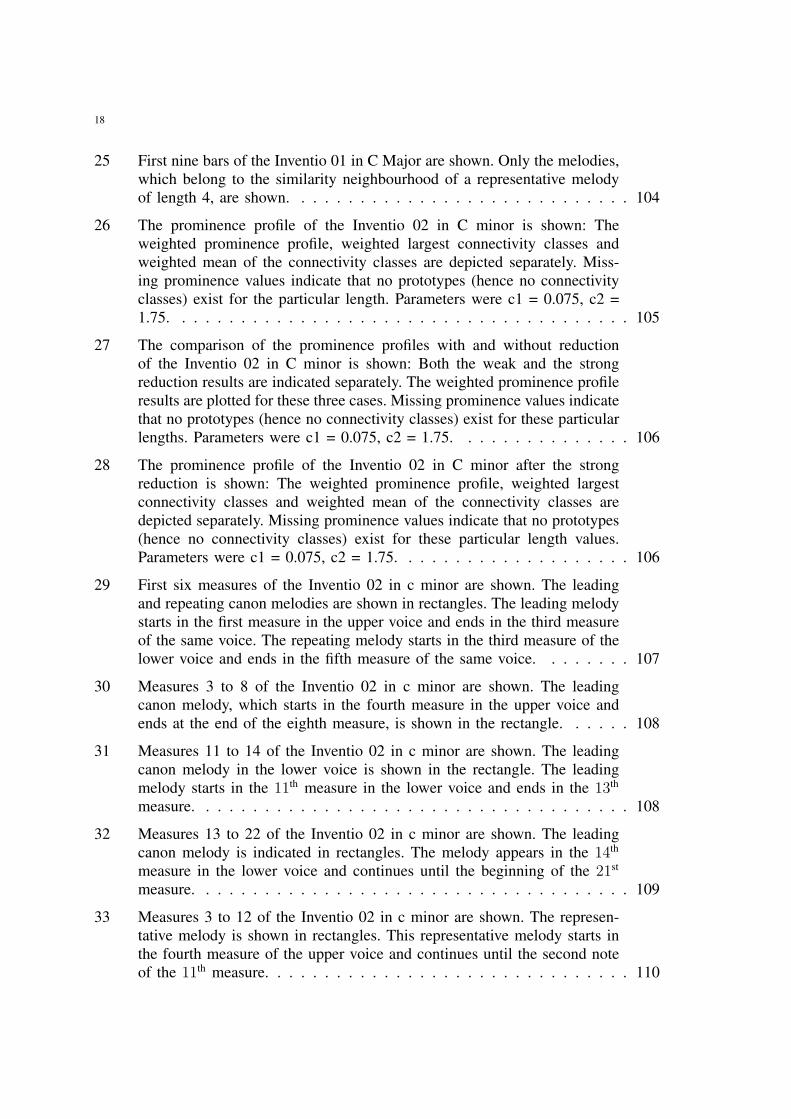
25 First nine bars of the Inventio 01 in C Major are shown. Only the melodies,which belong to the similarity neighbourhood of a representative melodyof length 4, are shown. . . . . . . . . . . . . . . . . . . . . . . . . . . . . 104

26 The prominence profile of the Inventio 02 in C minor is shown: Theweighted prominence profile, weighted largest connectivity classes andweighted mean of the connectivity classes are depicted separately. Miss-ing prominence values indicate that no prototypes (hence no connectivityclasses) exist for the particular length. Parameters were c1 = 0.075, c2 =1.75. . . . . . . . . . . . . . . . . . . . . . . . . . . . . . . . . . . . . . . 105

27 The comparison of the prominence profiles with and without reductionof the Inventio 02 in C minor is shown: Both the weak and the strongreduction results are indicated separately. The weighted prominence profileresults are plotted for these three cases. Missing prominence values indicatethat no prototypes (hence no connectivity classes) exist for these particularlengths. Parameters were c1 = 0.075, c2 = 1.75. . . . . . . . . . . . . . . 106

28 The prominence profile of the Inventio 02 in C minor after the strongreduction is shown: The weighted prominence profile, weighted largestconnectivity classes and weighted mean of the connectivity classes aredepicted separately. Missing prominence values indicate that no prototypes(hence no connectivity classes) exist for these particular length values.Parameters were c1 = 0.075, c2 = 1.75. . . . . . . . . . . . . . . . . . . . 106

29 First six measures of the Inventio 02 in c minor are shown. The leadingand repeating canon melodies are shown in rectangles. The leading melodystarts in the first measure in the upper voice and ends in the third measureof the same voice. The repeating melody starts in the third measure of thelower voice and ends in the fifth measure of the same voice. . . . . . . . 107

30 Measures 3 to 8 of the Inventio 02 in c minor are shown. The leadingcanon melody, which starts in the fourth measure in the upper voice andends at the end of the eighth measure, is shown in the rectangle. . . . . . 108

31 Measures 11 to 14 of the Inventio 02 in c minor are shown. The leadingcanon melody in the lower voice is shown in the rectangle. The leadingmelody starts in the 11th measure in the lower voice and ends in the 13th

measure. . . . . . . . . . . . . . . . . . . . . . . . . . . . . . . . . . . . . 108

32 Measures 13 to 22 of the Inventio 02 in c minor are shown. The leadingcanon melody is indicated in rectangles. The melody appears in the 14th

measure in the lower voice and continues until the beginning of the 21st

measure. . . . . . . . . . . . . . . . . . . . . . . . . . . . . . . . . . . . . 109

33 Measures 3 to 12 of the Inventio 02 in c minor are shown. The represen-tative melody is shown in rectangles. This representative melody starts inthe fourth measure of the upper voice and continues until the second noteof the 11th measure. . . . . . . . . . . . . . . . . . . . . . . . . . . . . . . 110

19

34 The prominence profile of the Inventio 04 in d minor before the reductionis shown: The weighted prominence profile, weighted largest connectivityclasses and weighted mean of the connectivity classes are depicted sepa-rately. Missing prominence values indicate that no prototypes (hence noconnectivity classes) exist for these particular lengths. Parameters were c1= 0.075, c2 = 1.75. . . . . . . . . . . . . . . . . . . . . . . . . . . . . . . 111

35 The comparison of the prominence profiles of the Inventio 04 in d minorwith and without reduction is shown: Both the weak and the strong re-duction results are indicated separately. The weighted prominence profileresults are plotted for these three cases. Missing prominence values indicatethat no prototypes (hence no connectivity classes) exist for these particularlengths. Parameters were c1 = 0.075, c2 = 1.75. . . . . . . . . . . . . . . 111

36 The prominence profile of the Inventio 04 in d minor after the strongreduction is shown: The weighted prominence profile, weighted largestconnectivity classes and weighted mean of the connectivity classes aredepicted separately. Missing prominence values indicate that no prototypes(hence no connectivity classes) exist for these particular length values.Parameters were c1 = 0.075, c2 = 1.75. . . . . . . . . . . . . . . . . . . . 112

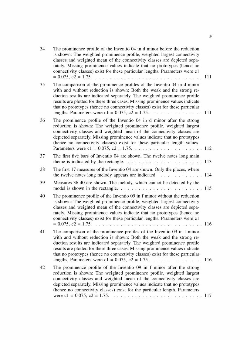
37 The first five bars of Inventio 04 are shown. The twelve notes long maintheme is indicated by the rectangle. . . . . . . . . . . . . . . . . . . . . . 113

38 The first 17 measures of the Inventio 04 are shown. Only the places, wherethe twelve notes long melody appears are indicated. . . . . . . . . . . . . 114

39 Measures 36-40 are shown. The melody, which cannot be detected by themodel is shown in the rectangle. . . . . . . . . . . . . . . . . . . . . . . . 115

40 The prominence profile of the Inventio 09 in f minor without the reductionis shown: The weighted prominence profile, weighted largest connectivityclasses and weighted mean of the connectivity classes are depicted sepa-rately. Missing prominence values indicate that no prototypes (hence noconnectivity classes) exist for these particular lengths. Parameters were c1= 0.075, c2 = 1.75. . . . . . . . . . . . . . . . . . . . . . . . . . . . . . . 116

41 The comparison of the prominence profiles of the Inventio 09 in f minorwith and without reduction is shown: Both the weak and the strong re-duction results are indicated separately. The weighted prominence profileresults are plotted for these three cases. Missing prominence values indicatethat no prototypes (hence no connectivity classes) exist for these particularlengths. Parameters were c1 = 0.075, c2 = 1.75. . . . . . . . . . . . . . . 116

42 The prominence profile of the Inventio 09 in f minor after the strongreduction is shown: The weighted prominence profile, weighted largestconnectivity classes and weighted mean of the connectivity classes aredepicted separately. Missing prominence values indicate that no prototypes(hence no connectivity classes) exist for the particular length. Parameterswere c1 = 0.075, c2 = 1.75. . . . . . . . . . . . . . . . . . . . . . . . . . 117

20

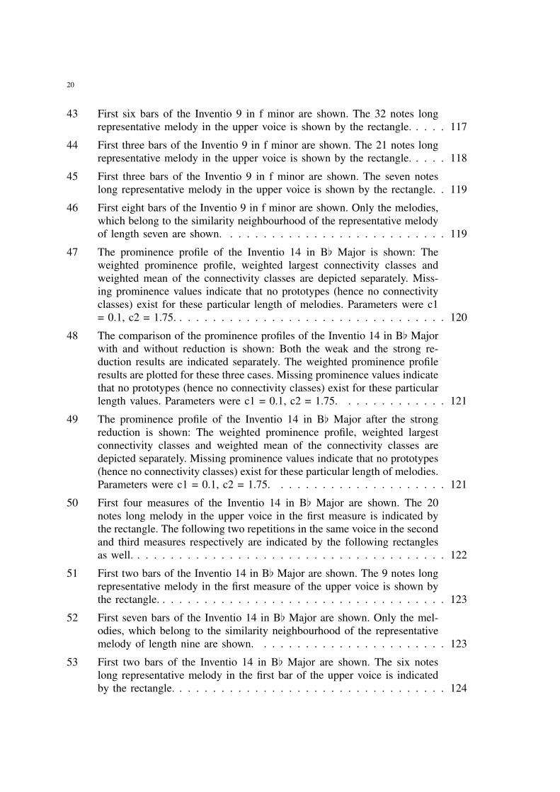
43 First six bars of the Inventio 9 in f minor are shown. The 32 notes longrepresentative melody in the upper voice is shown by the rectangle. . . . . 117

44 First three bars of the Inventio 9 in f minor are shown. The 21 notes longrepresentative melody in the upper voice is shown by the rectangle. . . . . 118

45 First three bars of the Inventio 9 in f minor are shown. The seven noteslong representative melody in the upper voice is shown by the rectangle. . 119

46 First eight bars of the Inventio 9 in f minor are shown. Only the melodies,which belong to the similarity neighbourhood of the representative melodyof length seven are shown. . . . . . . . . . . . . . . . . . . . . . . . . . . 119

47 The prominence profile of the Inventio 14 in B[ Major is shown: Theweighted prominence profile, weighted largest connectivity classes andweighted mean of the connectivity classes are depicted separately. Miss-ing prominence values indicate that no prototypes (hence no connectivityclasses) exist for these particular length of melodies. Parameters were c1= 0.1, c2 = 1.75. . . . . . . . . . . . . . . . . . . . . . . . . . . . . . . . . 120

48 The comparison of the prominence profiles of the Inventio 14 in B[ Majorwith and without reduction is shown: Both the weak and the strong re-duction results are indicated separately. The weighted prominence profileresults are plotted for these three cases. Missing prominence values indicatethat no prototypes (hence no connectivity classes) exist for these particularlength values. Parameters were c1 = 0.1, c2 = 1.75. . . . . . . . . . . . . 121

49 The prominence profile of the Inventio 14 in B[ Major after the strongreduction is shown: The weighted prominence profile, weighted largestconnectivity classes and weighted mean of the connectivity classes aredepicted separately. Missing prominence values indicate that no prototypes(hence no connectivity classes) exist for these particular length of melodies.Parameters were c1 = 0.1, c2 = 1.75. . . . . . . . . . . . . . . . . . . . . 121

50 First four measures of the Inventio 14 in B[ Major are shown. The 20notes long melody in the upper voice in the first measure is indicated bythe rectangle. The following two repetitions in the same voice in the secondand third measures respectively are indicated by the following rectanglesas well. . . . . . . . . . . . . . . . . . . . . . . . . . . . . . . . . . . . . . 122

51 First two bars of the Inventio 14 in B[ Major are shown. The 9 notes longrepresentative melody in the first measure of the upper voice is shown bythe rectangle. . . . . . . . . . . . . . . . . . . . . . . . . . . . . . . . . . . 123

52 First seven bars of the Inventio 14 in B[ Major are shown. Only the mel-odies, which belong to the similarity neighbourhood of the representativemelody of length nine are shown. . . . . . . . . . . . . . . . . . . . . . . 123

53 First two bars of the Inventio 14 in B[ Major are shown. The six noteslong representative melody in the first bar of the upper voice is indicatedby the rectangle. . . . . . . . . . . . . . . . . . . . . . . . . . . . . . . . . 124

21

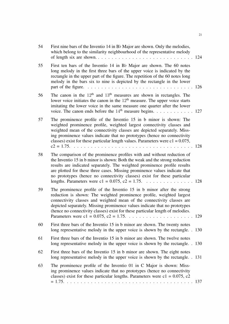
54 First nine bars of the Inventio 14 in B[ Major are shown. Only the melodies,which belong to the similarity neighbourhood of the representative melodyof length six are shown. . . . . . . . . . . . . . . . . . . . . . . . . . . . . 124

55 First ten bars of the Inventio 14 in B[ Major are shown. The 60 noteslong melody in the first three bars of the upper voice is indicated by therectangle in the upper part of the figure. The repetition of the 60 notes longmelody in the bars six to nine is depicted by the rectangle in the lowerpart of the figure. . . . . . . . . . . . . . . . . . . . . . . . . . . . . . . . 126

56 The canon in the 12th and 13th measures are shown in rectangles. Thelower voice initiates the canon in the 12th measure. The upper voice startsimitating the lower voice in the same measure one quarter after the lowervoice. The canon ends before the 14th measure begins. . . . . . . . . . . . 127

57 The prominence profile of the Inventio 15 in b minor is shown: Theweighted prominence profile, weighted largest connectivity classes andweighted mean of the connectivity classes are depicted separately. Miss-ing prominence values indicate that no prototypes (hence no connectivityclasses) exist for these particular length values. Parameters were c1 = 0.075,c2 = 1.75. . . . . . . . . . . . . . . . . . . . . . . . . . . . . . . . . . . . 128

58 The comparison of the prominence profiles with and without reduction ofthe Inventio 15 in b minor is shown: Both the weak and the strong reductionresults are indicated separately. The weighted prominence profile resultsare plotted for these three cases. Missing prominence values indicate thatno prototypes (hence no connectivity classes) exist for these particularlengths. Parameters were c1 = 0.075, c2 = 1.75. . . . . . . . . . . . . . . 128

59 The prominence profile of the Inventio 15 in b minor after the strongreduction is shown: The weighted prominence profile, weighted largestconnectivity classes and weighted mean of the connectivity classes aredepicted separately. Missing prominence values indicate that no prototypes(hence no connectivity classes) exist for these particular length of melodies.Parameters were c1 = 0.075, c2 = 1.75. . . . . . . . . . . . . . . . . . . . 129

60 First three bars of the Inventio 15 in b minor are shown. The twenty noteslong representative melody in the upper voice is shown by the rectangle. . 130

61 First three bars of the Inventio 15 in b minor are shown. The twelve noteslong representative melody in the upper voice is shown by the rectangle. . 130

62 First three bars of the Inventio 15 in b minor are shown. The eight noteslong representative melody in the upper voice is shown by the rectangle. . 131

63 The prominence profile of the Inventio 01 in C Major is shown: Miss-ing prominence values indicate that no prototypes (hence no connectivityclasses) exist for these particular lengths. Parameters were c1 = 0.075, c2= 1.75. . . . . . . . . . . . . . . . . . . . . . . . . . . . . . . . . . . . . . 137

22

64 The comparison of the prominence profiles with and without reduction ofthe Inventio 01 in C Major is shown: Missing prominence values indicatethat no prototypes (hence no connectivity classes) exist for these particularlength values. Parameters were c1 = 0.075, c2 = 1.75. . . . . . . . . . . . 137

65 A seven notes long melody from the Inventio 01 in C Major is indicatedby the rectangle. . . . . . . . . . . . . . . . . . . . . . . . . . . . . . . . . 138

66 The prominence profile of the Inventio 04 in d minor is shown: Miss-ing prominence values indicate that no prototypes (hence no connectivityclasses) exist for these particular length of melodies. Parameters were c1= 0.075, c2 = 1.75. . . . . . . . . . . . . . . . . . . . . . . . . . . . . . . 140

67 The comparison of the prominence profiles with and without reduction ofthe Inventio 04 in d minor is shown: Missing prominence values indicatethat no prototypes (hence no connectivity classes) exist for these particularlengths. Parameters were c1 = 0.075, c2 = 1.75. . . . . . . . . . . . . . . 140

68 The twelve notes long main melody of the Inventio 04 is shown. . . . . . 141

69 The prominence profile of Keren is shown: Missing prominence valuesindicate that no prototypes (hence no connectivity classes) exist for theseparticular lengths. Parameters were c1 = 0.075, c2 = 1.0. . . . . . . . . . 144

70 The comparison of the prominence profiles with and without reductionof Keren is shown: Missing prominence values indicate that no prototypes(hence no connectivity classes) exist for these particular lengths. Parameterswere c1 = 0.075, c2 = 1.0. . . . . . . . . . . . . . . . . . . . . . . . . . . 144

71 The piece is shown as a list plot, where the points indicate the notes andthe bindings are the intervals between consecutive notes. . . . . . . . . . . 146

72 The interval between the highest and the lowest note in the melodic unitwithin the first two measures of the piece is a tritone. . . . . . . . . . . . 146

73 Tritone interval between two consecutive notes in the second measure isshown. . . . . . . . . . . . . . . . . . . . . . . . . . . . . . . . . . . . . . 147

74 Tritone intervals in measure 8 are shown. The first note of this phrase,namely a B[ and the following note, which is an E constitute the firsttritone. The second tritone happens between the same E and the secondnote following this E, which is again a B[, an octave higher than the firstone. The third tritone is between the same B[ and the last note of theshown phrase, namely an E. . . . . . . . . . . . . . . . . . . . . . . . . . 147

75 Tritone interval between two consecutive notes in measure 20 is shown. . 147

76 The representative melody of length 16 in measure 24 is shown. . . . . . 147

77 The representative melody of length eight in measure 24 is shown. . . . . 148

23

78 The representative melody of length 22 in measure 40 is shown. Themelody is presented in its original metrical position and the eighth restbefore corresponds to notes appearing before the representative melodybegins. . . . . . . . . . . . . . . . . . . . . . . . . . . . . . . . . . . . . . 148

79 The representative melody of length 22 in measure 16 is shown. Themelody is in its original metric position. The quarter and eighth rests beforemelody correspond to notes appearing before the representative melodybegins. . . . . . . . . . . . . . . . . . . . . . . . . . . . . . . . . . . . . . 149

80 This figure shows the measures 40 and 41 of the piece, where yet anotheroccurrence of the latent two-voiceness can be observed. The first one isshown in Figure 79. . . . . . . . . . . . . . . . . . . . . . . . . . . . . . . 149

81 This figure shows measures 45 and 46 of the piece. The first tritone occursbetween the first note of measure 45, which is an E, and the B[, whichis repeated at the end of measure 45 and the beginning of measure 47three times. The last repetition of this B[ defines the next tritone with thefollowing note, which happens to be an E. Finally, the third tritone intervaloccurs between the same E and the B[ appearing at the end of measure46. Obviously the very first note of this phrase (E) and the last note (B[)define another tritone –up to octave. . . . . . . . . . . . . . . . . . . . . . 149

82 The spanning tritone interval in measures 47 and 48 is shown without anymetric specification. . . . . . . . . . . . . . . . . . . . . . . . . . . . . . . 150

83 The tritone interval in measure 54 is shown. . . . . . . . . . . . . . . . . 150

84 The spanning tritone interval in measures 61, 62 and 63 is shown withoutany metriic specification. . . . . . . . . . . . . . . . . . . . . . . . . . . . 150

85 A six notes long melody from the Inventio 01 is shown. . . . . . . . . . . 182

24

25

LIST OF TABLES

I The presence neighbourhood of the melody in the soprano part in Figure 13is shown. Each column represents a particular length of melodies thatcontain the given melody. L = 4 means the melodies listed in this columnare 4 intervals or 5 notes long. . . . . . . . . . . . . . . . . . . . . . . . . 72

II The presence neighbourhood of the melody in the bass part in Figure 13is shown. Each column represents a particular length of melodies thatcontain the given melody. L = 4 means that the melodies in this columnare 4 intervals long. . . . . . . . . . . . . . . . . . . . . . . . . . . . . . . 73

III Representative melodies with the highest significance values, number ofelements in their similarity neighbourhood sets, and number of melodiesin their connectivity classes for all two-voice inventions are shown. . . . . 132

IV The time needed to analyse a piece with and without the genetic algorithmsis shown for the whole corpus of Two-Voice Inventions. . . . . . . . . . . 136

V Topological investigation of the Two-Voice Inventions are shown. Thenumbers indicate lengths of melodies. For the cells, where two numbersare separated by a dash, the collections of the detected melodies, whoselength values are between these two numbers define topological bases. Thecells with single numbers in them indicate that the complete collections ofthe detected melodies define topological bases. . . . . . . . . . . . . . . . 163

26

27

I. INTRODUCTION: COMPUTERS ANDMUSIC

In the recent decades, a tendency emerged to study music in a scientific way. Froma musicological point of view, there is a reorganisation in music research, where musichas been started to be considered as a process of composing, analysing, performing andlistening. Hence, in these research studies, music as an acoustical phenomenon play acentral role [33].

After ignoring the research studies considering the spectral properties of music,computer aided music research can be divided into three main branches. These branchescan be named as “Music Composition”, “Music Cognition” and “Music Analysis”.

Music composition tries to model human behaviour, while human beings are com-posing music. This can be considered as an interdisciplinary research area. On the onehand, researchers try to find answers to questions concerning the act of composing. Thisact can be investigated from different viewpoints. Musicology investigates musical eras,compositional styles and their effects directly on music, on musicians and on listeners.Psychologists and neurologists model the psychological and / or neurological behaviourof the composers. On the other hand, this field is a research on aesthetic decision makingon how to choose the correct melodic, harmonic, and rhythmic passages to composemusic. Even-though there are several correct answers to a compositional problem, someof them sound better than the others. How composers make these decisions would bean interesting research question, considering all these disciplines mentioned in thisparagraph such as psychology, neurology, musicology, computer science etc. One finaland very technical viewpoint to music composition is the algorithmic composition,where researchers try to extract compositional rules, and re-apply them to imitate thecompositional styles.

Music cognition, on the other hand, tries to model human behaviour, while humanbeings are performing and / or listening to music. This research can be considered as aninterdisciplinary field as well. It is a well-known fact that written music and performedmusic do not match perfectly. The articulation of music differs from artist to artist.Depending on the articulation of the artist, but affected also by other factors, humanbeings perceive the same performance differently. Music cognition deals with questionslike what these factors are, which affect the perception of music directly and / orindirectly. However it is not only performance and perception of the performance, whatthe music cognition deals with. The composition side of music is also a field of interestof music cognition. Especially the auditory imagination of composers is a debated topicin cognition and neurology. Recent findings showed that imagination takes place in thebrain, where the perception takes place as well [41]. Neurological and psycho-acousticsresearch on musical memory also contributes to the cognitive research on composition.

28

The third branch, which combines these two research fields is the analysis of music.Analysis makes use of not only the progress made in the field of music composition,but also in the field of music cognition to understand how music emerges, not onlyacoustically but merely, systematically and phenomenologically. From the composi-tional point of view, analysis of music reveals the technical and stylistic details of acomposition, which in turn can be used to compose new musical pieces. Considering thefact that compositional styles or set of rules are nothing but just some common usages,a comparative study about the composers of the same era can easily reveal valuablefacts about the stylistic commonalities of this era. These findings can in turn be usedfor composing new musical pieces in the same style. In the composition departments ofmusic schools, this approach has been widely used to teach students how to compose.The students learn how to analyse music in order to be able to compose music. Fromthe cognition point of view, analysis of a musical piece figures out how composerscomposed music, which has been perceived as pleasant by the listeners. Artists makeuse of both of these viewpoints to structure their interpretation. They analyse a musicalpiece to understand its compositional details, which are supposed to lead them to thecognitive details of the same piece, so that they can construct their interpretation toconvey these details to the listeners in the best way.

The aim of the present study is to understand a given musical piece from both ofthese viewpoints, namely from the compositional and cognitive viewpoints, by analysingit melodically. Melody is one of the basic elements of music. Even untrained listenerscan repeat a well-known melody without making mistakes. However they certainly haveproblems in understanding the underlying harmony.

This study combines traditional analysis methods with computer aided and mathe-matical methods. Traditional analysis methods, which are used for several centuries arecombined with the semiotical and mathematical methods developed in the twentieth andtwenty-first centuries by using computers.

In the following, some preliminary studies about the music composition and cognitionare summarised briefly. The section following these two sections is dedicated to theanalysis of music. In the analysis section, traditional and modern analysis methods arementioned.

I.1. COMPOSITION

Since the development of computers, various attempts have been made to analyseand compose music algorithmically. Algorithmic music composition is one of the mostpopular areas of computer aided music research. Various artificial intelligence methodshave been used to produce music algorithmically.

In his long years of experimentation with algorithmic composition, Cope [21] devel-oped a rule-based expert system that uses methods of statistical inference to composetwo voice melodies in different styles. After recognising that music produced with thismethod is quite uninteresting, he revised his ideas. In his new approach [22] [23],he considered musical pieces as a set of instructions based on recombination. In an

29

oversimplified explanation, he divided a particular musical piece into tiny parts, andrecombined them in a logical manner using the instructions obtained from the piece.

Todd [69] developed a machine learning system to produce one-voice melodies. Thiswork is among the various attempts making use of machine learning methods thatsuccessfully produces music. It suffers, however, from repetition of the same group ofnotes. Mozer [57] used a connectionist approach to compose one-voice melodies. Hestarted with the ideas of Todd and enhanced them to create a better system. He useda novel method to represent pitch and duration. Both systems developed by Todd andMozer can produce one-voice melodies only. Hild [31] and Hornel [34] designed aconnectionist system similar to the work of Todd to re-harmonise Bach chorales. In thissystem, an artificial neural network was developed to determine the harmonic functions.Some generic algorithms were used to compose the accompanying melodies dependingon the determined harmonic functions. Another work accomplished by Widmer [71]introduced a system producing first species counterpoint [29] pieces. He used a databaseapproach in this work. Because stylistic concerns were not embedded into the system,it did not produce expected melodies.

Adiloglu and Alpaslan [1] [2] concentrated on the representation of pitch and durationusing feed-forward neural networks as the knowledge representation method. From thisviewpoint, this study aims to enhance the work introduced by Mozer by making use ofan efficient representation of pitch and duration to produce polyphonic pieces.

I.2. COGNITION

Music cognition is an interdisciplinary research field to understand music as a mentalprocess, where perception, comprehension, memory, attention are several aspects, whichare considered separately and / or together to figure out how the mind senses music.Topics in this field include perception of grouping structures like motives, melodies,phrases, perception of rhythms and meter, musical similarity and expectation, musicalperformance, etc.

In research fields related to perception, observing and collecting data is extremelyimportant, so it is in music cognition. Formalisation of the collected data, which hasbeen obtained by performing these empirical studies is as important as collecting thedata. The conclusions drawn from these formalisms tend to consider the music theoryas their central point and either derive alternative methods to the traditional musictheory or try to validate their results by using music theory. Theories making use ofthe formalisation paradigm are generally computational models. These models are welldefined in a given scope, are testable, hence they can be validated by testing on severaldifferent corpora. Even applying them on a corpus, which has not been aimed at duringthe development of the model can yield interesting results or raise interesting questions.The generative theory of tonal music by Lehrdahl and Jackendoff [45] is a well knownexample of such models.

The development of empirical and computational models is the new trend in thewhole cognitive research field. In the music cognition sub-domain, researchers like

30

Krumhansl [42] worked on perception of tonal centres. In her studies, Krumhansl foundout that in a tonal context, the most stable pitch is the tonic, followed by other pitchesof the tonic triad, followed by the remaining scale tones, followed by the non-scaletones. This four-level response pattern is called by Krumhansl the ”tonal hierarchy“. Incase of consecutive pairs of different pitches, human beings are more likely to perceivethem as being closely related, if both pitches are rated highly in the tonal hierarchy.On the other hand, the perceptual distance is closer between two consecutive pitches,when the second pitch is more stable in the tonal hierarchy than the first one. Hence,the distances between the consecutive pitches are asymmetric. Huron [35] discusses inhis review of the book of Krumhansl, whether these pitch transitions have been morecommonly used in typical melodies. In his experiments, he found out that there is nosignificant difference between the pitch relatedness values of a given melody and itsretrograde.

While Krumhansl has worked on pitches and keys, Parncutt [63] has tried to explainthe western harmony using psycho-acoustical principles. From an historical viewpoint,his attempt is a modern interpretation of Rameau’s theory of harmony derived from asingle tone. In this respect, Parncutt derives his model based on the perception of a singletone. Departing from the fact that both tone and chord are vertical sounds, he definesa perceptual relationship between tone and chord. In his model, Parncutt defines staticproperties of sounds like tonalness, multiplicity and salience. Tonalness is the degree ofthe sensation of a single tone, which a sound evokes. Multiplicity defines the numberof evident tones in a sound. Lastly, salience is the perceptual noticeability of a pitch ina sound. The saliency values can be summed up for each chromatic category in a scaleto find the fundamental of a given chord in a psycho-acoustical way. Parcutt definesalso dynamic values to explain the successive chords or chord progressions based onthe pitch commonality. Finally, he can define the overall consonance of a given chordprogression. Building up the model in this way, he introduced a conceptual languageto explore musical harmony.

I.3. ANALYSIS

Listening to music is a complex phenomenon. Through the long evolution history,animals have evolved to hear and communicate through sounds. However human beingshappen to be the only species in the world, who can perceive music, because the humanbrain can process complex patterns of sounds [41]. Starting with the smallest pattern,we can analyse pattern by pattern, until we reach a complete symphony. On the onehand, consecutive tones constitute a part of a melody, which in turn constitute a melody.Melodies come together to construct phrases, which the passages are comprised of. Inthe vertical direction, on the other hand, two simultaneous tones produce intervals.At least three simultaneous tones build chords, which in turn makes three simultaneousintervals. Finally consecutive chords are considered as harmonic progressions. In a thirddimension, different length of tones and beats are perceived as different rhythms. Evenloudness has different meanings, which are important, in order to articulate a givenmusical piece in a correct way. Hence, music is a complex phenomenon, which is a

31

combination of all these dimensions, which are processed in human brain accordingly.Each of these dimensions is a complex phenomenon on its own way.

Considering each of these phenomena, in order to produce and understand music,several techniques have been developed throughout the history. In this thesis, I willnot consider the production of music, but concentrate myself mainly on analysis ofmusic. In fact, being able to analyse music contributes in turn to be able to produce(compose) music. Therefore, the ability to analyse a given musical piece is one of thebasic specialities, which a human being should possess to be able to compose music.

Analysis of a musical piece is composed of several analysis steps, which cannotbe considered independent of each other. In order to perform a complete analysis of agiven piece, the given piece should be analysed from a melodic, harmonic and rhythmicviewpoints. Considering the places, where melodies appear, the relative positions andthe order of them, the form of the piece should be determined as well.

Through the centuries, parallel to the technological and cultural development, musichas evolved as well. Not only different genres emerged, but certain musical genresalso changed. These changes appeared sometimes as improvements of the compositiontechniques, but also sometimes as reaction to the previous era. As an example of thelatter phenomenon, the fourths were considered to be dissonant in the early music.However, starting with the renaissance, the same interval was considered to be consonantat once.

All these aspects should be considered during the analysis process. A certain analysisprocedure is, because of these facts, not applicable to all different types of music.Therefore, analysis methods have also been improved throughout the history. Not onlybeing able to understand the development of the music, but also being able to improvethe process of analysis so that a given piece can be analysed in a more comfortable andin turn fast manner.

In the following sections, I will introduce different analysis methods briefly, whichhave influenced this thesis in a certain way.

1. Traditional Analysis Methods

Music theory is a well established discipline which provides several techniques toanalyse a piece of music completely. A piece of music is analysed - usually by handand using expert knowledge - by extracting and integrating information about melody,harmony, rhythm, meter and form. The analysis of a given piece is generally viewed asan inseparable process, which must link different elements and levels of description.

1) Melodic Analysis: In the literature of music, two terms motive and melody are usedinterchangeably. A motive is generally defined as the smallest musical unit, which hasan individual expressive meaning [65] [25]. It is the germinal unit in a given music piecewith an individual character, which constructs the melodies of the given piece. However,melodies can also appear without containing a germinal motive in the given piece.A motive is considered in some definitions as a rhythmic unit without regarding the

32

intervallic relations between the consecutive notes [64]. In order to avoid the conflicts,I will use the term melody in the rest of the dissertation for two reasons: On the onehand, this dissertation entails a research on melodies as combination of motives. On theother hand, I ignore the rhythmic features of notes and in turn melodies.

Melodic sequences are localised musical structures, which on the one hand inherittheir significance from the organisation of the whole piece and which, on the other handcontribute to the constitution of the piece by their repetitions and variations. Melodicanalysis interacts with other analytical aspects such as the manifestation of harmonicprogression in the voice leading.

From the amateur listeners point of view, melody is the very first recognisable andeasy to remember element. Neurological findings tell us that the auditory cortex onthe right hemisphere of our brain is responsible for the melodic sequences, when theamateur listeners are concerned. However, for the more experienced listeners, the lefthemisphere takes over this responsibility [41]. An amateur listener recognises a melodyas a whole, without paying attention to the harmonic structure of it or considering thesmaller components of a melody. However a professional musician listens to music ina different way. A professional musician makes a comparative analysis of a melody,which he / she just listened to from different view points so that he / she extracts theharmonic and rhythmic structure of the melody at once. But in any case, melodies aretone sequences, where the consequent relations of individual tones play an importantrole. The consequent tones are perceived separately in the brain, but combined togetherin a certain melody. However, this does not happen always. The neuroscientists, psycho-acousticians, musicologists, but especially the composers have dealt with the problemfor centuries, about what makes a tone sequence a melody.

In different parts of the world, music is based on different tone scales. In the westernmusic, after a long development period, the major and minor scales were established. Amajor or a minor scale is comprised of eight tones according to a certain interval pattern,where the eighth tone is the repetition of the first. In the equi-tempered intonation,with the accidental tones, it makes twelve tones in total, which makes chromatic scalecomplete. In other intonation systems like the well-tempered, middle tone or others,a flattened note does not correspond to the sharpened note, one position below theflattened note in the tone scale. However these differences have not frequently beenused in the compositions. Especially in the early periods of music, before micro-tonalmusic emerged, a suitable intonation system has been chosen to tune the instruments,where these differences cannot affect the performance of the piece badly. However, indifferent cultures, different tone scales are used for making music. A popular example isthe Gamelan music, which is based on a pentatonic (five tones) tone scale [50]. Anotherexample is the Turkish music. The Turkish music is based on a large number of differenttwelve tone scales, where the micro-tonal intervals are also important [61] [62]. Thenumber of these examples can increase easily.

Assigning individual tones to a single melody is not an inherited feature. Peoplerather get used to certain tone sequences, based on certain tone scales during their life.Therefore, listening to music, which is based on a different tone scale sounds mostly

33

disturbing. However, there is one common feature for all these different traditions,when the melody is concerned, namely the contour of a melody. No matter, which tonesequence a melody is based on, listeners recognise the contour of a melody at first place.There is even no difference between a professional musician and an amateur listener inrecognising the contour of a melody [41].

Despite all this information, even the contour does not answer the question, whatmakes a tone sequence a melody. Based on different research disciplines, there is acommon answer to this question, which does not depend on different music traditions:The tones of a melody are mostly comprised of neighbouring tones of a tone scale.Short jumps are used rarely. Long jumps should be used very carefully, because theyare generally perceived as the end of a melody. The rests also make difficult to followup a melodic contour. Therefore they are perceived as the end of a melody as well.However, in order not to be monotone, too many repetitions of the same tone should beavoided. The highest and the lowest tones of a melody should appear preferably onlyonce [41]. Rhythmic changes should mainly appear in upbeats.

In a western composition, some additional commonalities exist, which the traditionalharmonic and formal structures introduce. Especially the tone scale, the consonant anddissonant intervals, harmonic resolutions and the form affect the melodic progress aswell as melodic progressions affect these in return. Therefore, analysis of a givenmusical piece is an interchanging process, which should consider all these aspects of acomposition. Therefore, in the following two sections, I will introduce the formal andharmonic analysis of a given music piece from a melodic point of view.

2) Harmonic Analysis: The harmony is generally considered as the vertical relation-ship of the notes, which sound simultaneously [51] [52]. In the history of music, ithas been a continuous process in time in which the harmony and the harmonic ruleshave emerged. In the very beginning of the polyphony, melodies were song parallelto each other starting with an interval, generally of a third. As time passed, the art ofparallel singing was varied, and harmonic rules started to emerge, in order to rule howto apply these variations into these parallel voices. However, these rules have neverbeen dictated by certain experts in a certain period, but they have always been commonusages in the compositions. Therefore there were exceptions to these common usages.Comparing these common usages in different periods, it is easy to find contradictingrules. Therefore, when a music piece is going to be analysed, the period in which thepiece was composed should be considered.

In the historical development of the polyphony, firstly, the horizontal relationshipsof notes were considered to be important without ignoring the vertical relationshipsof notes. This compositional style is called the counterpoint, which can be interpretedas note-against-note composition [40]. In the counterpoint composition, the horizontaldevelopment of music is important, where each horizontal line, each voice or part, is anindividual value for the composition, and all these single parts together constitute thewhole composition. The relationships of the notes within the same part and also betweenthe parts were categorised as consonant, pleasant intervals, and dissonant, displeasingintervals. Hence, the counterpoint composition was about how to introduce dissonant

34

intervals, and how to resolve them into consonant intervals. In general, dissonant in-tervals bring local stress points into the composition, which should be resolved intopleasant intervals, which in turn remove these stress points and create a kind of relief.Several variation techniques were developed in this compositional style, in order to varymelodies. Especially, the melodic variations, which will be explained in detail in thefollowing sections like inversion, augmentation, diminution and retrograde are widelyapplied techniques in the counterpoint composition.

During the centuries, the vertical relationships between the notes became more andmore important compared to the horizontal relationships. The composers consideredthe vertical progress of the composition as well as the horizontal development. So,the chords and the chord progressions became important. After the establishment ofthe tonal system, the modulations between the tonalities became the state of art forcomposition. The composers found ways to move from one tonality to another, and howto settle the new tonality, namely via cadences. However, the horizontal developmentof the music was not left immediately. Especially J. S. Bach was one of the masters ofa composition technique called harmonic counterpoint, where both the horizontal andvertical progression of the music was equally important. However, as the time passed,vertical development of a musical piece became more important than the melodic lineswithin a musical piece.

From a cognitive view point, vertical relationships within a musical piece are moredifficult to perceive or to understand than the melodic relationships [41]. Therefore,it is quite difficult to follow the harmonies within a musical piece, although even thebeginners can follow melodies. But from a music theoretical viewpoint, melodies andharmonies affect each other during the development of a musical piece, so that themelodies and the harmonies are adapted to each other. In other words, one is changedaccording to the other within the whole piece. Therefore, when performing a melodicanalysis, harmonic analysis is required, in order to be able to explain why a melodyhas been varied from the original appearance during the piece.

3) Formal Analysis: Melodies and harmonies are local structures within a musicalpiece. However, the form of a musical piece is a global structure, which brings a certainorder into the piece. On the one hand, the melodies and the harmonies find their placesin this global structure. On the other hand, these local structures gathered together definethe global form of a piece. Hence, as it has been the case between melody and harmony,there is a mutual interaction between melody, harmony and form.

In general the form of a musical piece has three characteristics, the tone material,the gestalt principles, and the ideas [51]. The tone material of the form is the physicalmaterial, which a composer uses to generate his / her composition. The tone material ismostly restricted by the planned composition. When a composer is composing a choral,the highest and lowest notes, which human beings can sing restricts the composer. Thismaterial restriction directly affects the melodic and harmonic progression of the musicalpiece. On the other hand, the duration of the tones, the loudness and the tone colourare parts of the tone material of a musical piece as well. However, these are secondarilyimportant in the harmonic analysis of a musical piece. Even-though duration of the notes

35

is important in the melodic analysis, the other two can be considered to be secondarilyimportant for the melodic analysis as well. They rather affect the performance and inturn the perception of the musical piece more directly.

The gestalt principles of a musical piece are mainly aesthetics-related, in order tobalance the contrasts with the repetitions within a musical piece. Partitioning of amusical composition is of an importance for the perception of the piece [51]. Thehuman memory needs a skeleton of a musical piece, in order to understand the piece ina better way. Hence, the form of a musical piece is an abstraction of the model of thepiece, which tries to explain the structural connections between the parts of a musicalpiece. Even-though a form of a musical piece is an abstracted model, it is individualfor each single musical piece. Therefore a formal analysis of a given musical piece isrequired to understand these connections in a better way.

Within the gestalt of a given piece, creative ideas make a musical piece individual.Without violating the formal structure of a given piece, these ideas help to develop singlepartitions of the form, and define the connections between them. From this viewpoint,these ideas generate the melodies and harmonies, and in turn the content and the bordersof the formal elements of a composition. Hence, by forming the partitions and in turnthe whole piece through these creative ideas , the mutual relationship between melody,harmony and form shows itself in a very clear way. Therefore, the analysis process ofa given musical piece is an inseparable process of the melodic, harmonic and formalanalysis.

2. Alternative Analysis Methods

1) Music Semiotics: An alternative approach to standard music theory was proposedunder the discipline “semiotics of music” [56]. In this approach, attempts were made toreduce the subjective elements of music analysis and to disentangle the analysis process.

Semioticians distinguish between paradigmatic and syntagmatic aspects of a complexsign, such as a text or a piece of music. Under the paradigmatic view, the elements of apiece and the role they play are defined by considering their individual properties and byrelationships based on transformation and similarity (or dissimilarity). The syntagmaticview then covers information extracted from the (spatial) context within which theelements appear, and how they sequentially (or spatially) relate to each other. Underthe semiotic approach, the paradigmatic analysis of a piece ideally leads to the definitionof musical elements (or at least promising candidates) followed by a segmentation (ora more general syntagmatic structure) of the piece on which the advanced syntagmaticanalysis can be based. These methods can be applied universally to all music styles,where the formal or paradigmatic repetition of small and large units plays an importantrole. However, this is not to say that these conditions are universal to any musical style.

The approaches of Nicolas Ruwet [67] and Jean-Jacques Nattiez [59] depart fromparadigmatic criteria, in order to obtain suitable segmentations of a given piece.

Ruwet [67] proposed an algorithmic strategy to identify paradigmatic units in a givenpiece. In this approach, attempts were made to reduce the subjective elements of music

36

analysis and to disentangle the analysis process. Nattiez [59] refined this semioticapproach and characterised it as a type of analysis on the neutral level, aside frompoietic and aesthetic aspects. The present approach strongly resonates with Ruwet‘soriginal proposal in the sense that our proposed paradigmatic methods are a prerequisiteto further work to be done on the syntagmatic domain.

Ruwet: A Machine to Discover Paradigms: The melodic structure of a givenmusical piece is a hierarchical organisation in the sense that larger structures are dividedinto smaller structures even in simple musical pieces. Therefore, as a result of a musictheoretic analysis [65], a musical piece is divided into parts on different levels. Ingeneral, a musical piece can be divided into periods, which in turn into phrases, etc.

Ruwet [67] claims that it is uncertain, whether the concepts like period, phrase areuniversal or specific for particular pieces, and change their meaning from piece to pieceslightly. More important than that, he claims that no one tries to answer the question,which criteria are the crucial ones to perform this kind of a segmentation:

“What are the criteria which, in such and such a case, have presided overthe segmentation?”

His answer to the question above is repetition. In his model “a machine for discover-ing paradigms”, Ruwet uses the repetition as his main principal of division. Repetitionindicates the significance of melodic segments, which appear at different places withina given musical piece. Therefore, in his model, he analyses the repeated passages tosegment a given piece. While doing this, he mainly uses three basic rules:

• The longest passages that are repeated fully are identified.• Passages that are not the same at first sight may be transformations of each other.• If pitch and rhythm are separated, we may obtain similar contours with different

rhythms or similar rhythms with different contours.

He applies these rules as a quite flexible algorithm to the musical pieces to find thesignificant segments of them. In his analyses, he considers only the pitch and durationidentity, the other attributes of musical notes are ignored. As also implied by the thirdrule, he separates these two attributes to make a deeper analysis if necessary.

Nattiez: Extensions to Ruwet’s Model: Another semiotician, Nattiez [59] improvedthe model introduced by Ruwet, and called the improved version “neutral level” [56].The neutral level is the analysis of music without considering the poietic and aestheticmatters. In other words, what the composer means and what the listener perceives areunimportant on the neutral level, only what in the score is given is considered. Both ofthese approaches are intuitive approaches. In other words, they are not implemented ascomputer programs but performed by hand. Nattiez further claims that it is impossibleto implement the neutral level as a computer program.

2) Music Information Retrieval: Especially paradigmatic aspects have been investi-gated by using some computer aided information retrieval methods. Different approachescan be categorised in two main groups.

In the first group, researchers develop methods to identify similarities between musical

37

objects like melodies, rhythm, etc. These approaches do not aim at investigating musicalpieces. In the second group, researches aim at analysing entire pieces form a certainlevel of description like melody. Lemstrom and Ukkonen [46] defined a translation-invariant edit distance, which can automatically recognise the translations of melodieswithout using an interval based encoding. They embedded interval encoding into thecost function of the distance measure. The cost function is also able to consider thecontext containing the melodies, while the similarities are calculated. However, they didnot define a global framework to extract the melodic structure of a given piece froma music-theoretical point of view, but rather, given a melody, searched places within ahuge melody-database, where the given melody appears.

The second group of approaches considers music pieces entirely, which containmelodies as sub-segments of this ambient space. Lartillot [43] [44] defined a musicalpattern discovery system motivated by human listening strategies. Pitch intervals areused together with duration ratios to recognise identical [44] or similar [43] note pairs,which in turn are combined to construct similar patterns. The selection of patterns isguided by paradigmatic aspects, and overlaps of segments are allowed. Cambouropou-los [16], on the other hand, proposed methods to divide given musical pieces intomostly non-overlapping segments. A prominence value is calculated for each melodybased on the number of exact occurrences of non-overlapping melodies. Prominencevalues of melodies are used for determining the boundaries of the segments [17]. Healso developed methods to recognise variations [16] of filling and thinning (throughnote insertion and deletion) into the original melody. Cambouropoulos and Widmer [18]proposed methods to construct melodic clusters depending on the melodic and rhythmicfeatures of the given segments. Basically, similarities of these features up to a particularthreshold are used to determine the clusters. High computational costs of this methodmake applications to long pieces difficult.

3) Mathematical Music Theory: Mazzola [48] [49] and Buteau [14] [15] proposeda general theoretical framework for the paradigmatic analysis of the melodic structure,which is driven by the idea that a paradigmatic approach, where relevant melodicelements can be identified in terms of the richness of paradigmatic relations amongeach other can be formulated in terms of topology. They consider not only consecutivetone sequences, but allow any subset of the ambient melody to carry a melodic shape(such as rigid shape, diastematic shape, etc.). Paradigmatic relations are composed oftwo kinds, namely symmetry transformations, which map one shape to another and apseudo-metric, which measures the similarity of melodic shapes. The approaches ofMazzola and Buteau are convincing from a mathematical point of view, but radicalfrom a music-theoretical one. The consideration of all tone sets as candidates formelodically significant elements leads to high computational efforts and difficulties inthe interpretation of the complex results. The computational difficulties were handledby limiting the candidate sets of tones to fall into a sliding window of a given sizewith the risk to loose important melodic elements. In order to be able to interpret themathematical results, Mazzola and Buteau introduced advanced topological structures,which accumulate the paradigmatic relations for varying similarity degrees in a tree. Inthe light of the mathematical rigor of these two approaches, it is desirable to have many

38

applications in music analysis, in order to eventually evaluate their music-theoreticalrelevance.

The approach of Buteau is being integrated into the Open Music software of IRCAMCentre Pompidou [39], which is a visual programming environment to compose andanalyse music.

Another valuable study in paradigmatic melodic analysis was done by Nestke [60],who focuses entirely on symmetry-based paradigmatic relations, and excludes similarityup to a particular threshold. In this restricted mathematical universe, he was able toovercome the computational limitation of a sliding window. He also offered refinedcombinatorial methods for a sub-sequent syntagmatic analysis in terms of simplicialcomplexes and their homology. These structures serve to measure the complexity of theimplied syntagmatic structures. Also this approach needs to be evaluated with respectto its music-theoretical relevance.

These ideas of Nestke were implemented in the in the program MeloPatch or as aplugin to the software RUBATO [53].

Nestke also mentions the Hausdorff distance to measure the resemblance of two sets.He suggests that this metric can be applied to calculate the function melodic weight,which measures the importance of a tone in a melody with respect to a chosen paradigm.

All of these three research studies construct melodic structures based on melodicpatches. A melodic patch is a subset of a melody containing not only consecutivenotes. Therefore, the amount of the melodies and melodic relations these three modelsare supposed to analyse grow exponentially. This in turn causes that these models yieldlarge amount of information to post-process. It is difficult to evaluate this amount ofinformation provided by their analyses. Furthermore, the results of these models containa lot of melodies consisting of non-consecutive notes, which is difficult to interpretmusic-theoretically as well.

I.4. COMBINING MATHEMATICAL, SEMIOTICAL AND INFORMATION RE-TRIEVAL APPROACHES

In this thesis, I address the melodic analysis of music pieces by combining ideasfrom traditional- and mathematical music theory, music semiotics and music informationretrieval in a harmonious way. I introduce a mathematical model inspired by semioticalideas of Ruwet and Nattiez to extract the melodic structure of a given music piece.Hence, I do not consider, how melodies are perceived by human beings, but concentratemyself on the neutral level of the given piece. The model is mathematically sound, butkept as simple as possible. To be precise, in this study, I considered only melodiesconsisting of consecutive notes. Due to this decision, the method does not suffer underthe sliding-window limitation. Besides, the amount of the results are tractable. I admitthat this also implies a risk to loose important melodic elements. But since melodicsegments are much easier to interpret in music-theoretical terms than non-contiguoussets of tones, this strategy potentially allows evaluating the results in comparison with

39

standard music-theoretical analysis. Hence, the results are justifiable from the musictheoretical viewpoint as well. Therefore, in this thesis, the results obtained from themodel are presented in a traditional music-theoretical context indicating these similaritiesand how these similarities contribute to the form of the given piece.

The model extracts the melodic structure of a given music piece in a paradigmatic way.However, it does not suggest a certain segmentation for the given piece, but just indicatesespecially the similarity relations between melodic segments including their locationswithin the given music piece. In other words, I prefer grouping the similar melodies,instead of segmenting, which is also reminiscent of Lartillot [43], [44]. In my approach,segments can overlap or even contain each other. I search the similarities betweenmelodies, and construct a global melodic landscape, which stands for the paradigmaticmelodic structure of a given piece.

Even-though I combined these well-established research fields in this study, due to thefact that it is a computational model, there are some inevitable assumptions I have made,which caused that some parts of the results do not converge to the music theoreticalresults. However, I do not present the so-called music theoretically “correct” resultsas true-positives and the others as false-positives as it is usually done in the field ofmusic information retrieval. In this study, I do not present some percentages of the musictheoretically relevant results, which are supposed to indicate the success of the presentedmodel. Instead, I indicate these places, and explain the causes of them. In music, there isnot a ground truth always. Hence, compositions and their analyses are mostly opinionssupported by some other opinions. Therefore, I believe that explaining the reasons,instead of giving dry numbers makes much more sense as far as music is concerned.Furthermore, the places, where these divergences occur are worth investigating. Theexplanations of the reasons why they occur throw new research questions.

The thesis is composed of four main parts. In the first part (Chapter II), followingthis introduction, I present the model, which I call the similarity neighbourhood modelin detail. In this chapter, I define necessary musical and mathematical concepts, whichI used throughout the model. I discuss the pros and cons of alternative methods, andexplain the reasons of my decisions in those cases. I introduce my similarity concept, theevaluation of the melodic material given within the given musical piece, hence melodiesand their sub-melodies, and finally how I fine-tuned the extracted melodic structure forthe given musical piece.

The second part (Chapter III) introduces an approximation to the similarity neigh-bourhood model, which aims to accelerate the model without loosing the essential infor-mation provided by the model. An evolutionary approach called the genetic algorithmsare presented in this part of the thesis.

The third part (Chapters IV, V and VI) introduces the analyses performed by themodel and the obtained results. The results are presented in a music-theoretical way, sothat the relevance of the results with the traditional methods becomes clear. I presentanalysis results of some of the Two-Voice Inventions of J. S. Bach [12] as representativesof the compositional styles in Baroque music. In order to observe the generalisibilityof the model, I present the analysis results of a modern musical piece, namely Keren

40

of I. Xenakis [72].

The fourth part (Chapter VII) investigates the mathematical features of the similarityneighbourhood model. It is a relatively theoretical part of the thesis. In this part, I revisethe results I have presented previously from a theoretical point of view depending onthe findings made in this part.

A concluding chapter finalises the thesis, where I comment on the whole model con-sidering the theoretical as well as the practical findings gained. Furthermore, analogiesbetween a philosophical study and the similarity neighbourhood model are mentionedas well.

41

II. THE SIMILARITY NEIGHBOURHOODMODEL

II.1. INTRODUCTION

In the context of this study, I introduce an analytical model, which provides detailedinformation about the melodic level of description of a given score without referenceto external expert knowledge.

The method, which I call the similarity neighbourhood model is based on a “rel-ative pitch”-representation of a piece of music. In this method, similarity rather thansymmetry is used for determining the proximity. In other words, the proximity of twomelodies is measured by means of a similarity measure. By counting the number of closeneighbours of a given melody in the piece as a measure of significance, those melodiesare identified as prototypes, which appear more often than a given threshold value. Themelodies are clustered in connectivity classes according to a transitivity principle. Forevery cluster, a representative melody is chosen out of the largest neighbourhood set.All similarity classes including non-prototypical ones - have a topological refinementin terms of the intersection sets (i.e. intersections of neighbourhoods) which defines atopological base.

The sub-melodic relationships are investigated by using the proximity relations aswell as the positions of the melodies within a given piece. Hence, not only the intervalsequence based on the relative-pitch representation, but also the position information ofa melody is incorporated to perform the analysis.

The similarity relations and the sub-melodic relations together yield the melodicprofile of a given piece. The so-called prominence profile indicates the prominence ofthe melodies in a summarised manner.

Consequently, the similarity neighbourhood model is a hierarchical model, built on ba-sic similarity relationships of melodies. The similarity relationships of melodies dependin turn on the representation and the similarity concept. Therefore, in the following,I introduce the representation scheme I used for defining melodies followed by thesimilarity concept.

II.2. DEFINITION OF MUSICAL CONCEPTS IN MATHEMATICAL TERMS

The equality relation between melodies is a useful but very narrow relation to extractthe melodic structure of a piece. A sizeable part of the information about the evolution ofa melody gets lost, because of the insensitivity of the equality against melodic variations.Here, to solve this problem, I utilise a similarity measure.

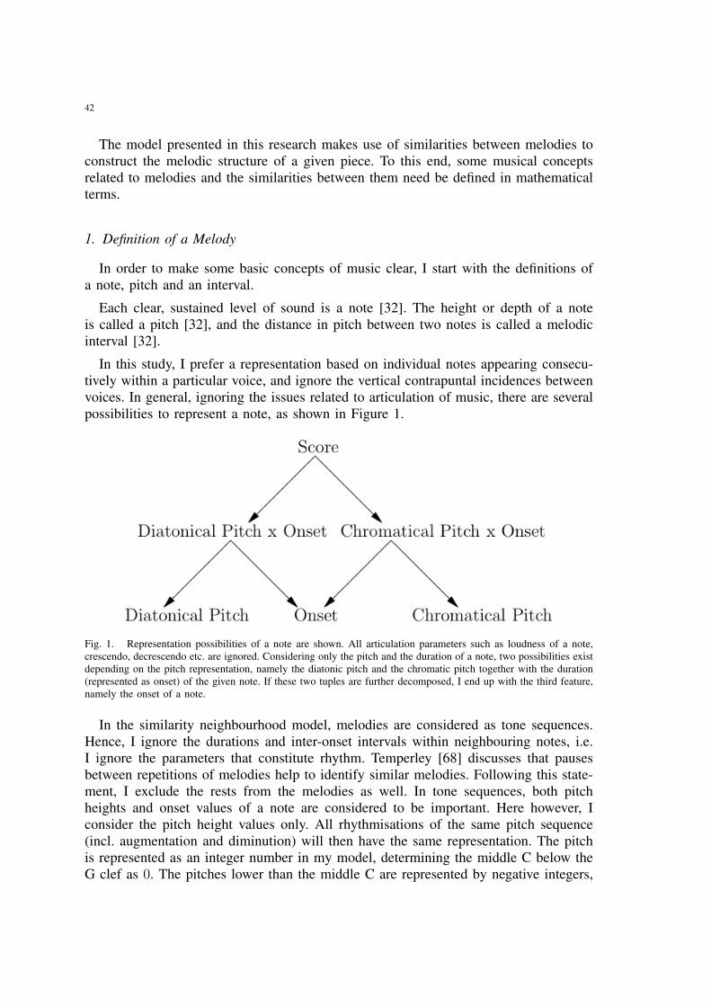
42

The model presented in this research makes use of similarities between melodies toconstruct the melodic structure of a given piece. To this end, some musical conceptsrelated to melodies and the similarities between them need be defined in mathematicalterms.

1. Definition of a Melody

In order to make some basic concepts of music clear, I start with the definitions ofa note, pitch and an interval.

Each clear, sustained level of sound is a note [32]. The height or depth of a noteis called a pitch [32], and the distance in pitch between two notes is called a melodicinterval [32].

In this study, I prefer a representation based on individual notes appearing consecu-tively within a particular voice, and ignore the vertical contrapuntal incidences betweenvoices. In general, ignoring the issues related to articulation of music, there are severalpossibilities to represent a note, as shown in Figure 1.

Fig. 1. Representation possibilities of a note are shown. All articulation parameters such as loudness of a note,crescendo, decrescendo etc. are ignored. Considering only the pitch and the duration of a note, two possibilities existdepending on the pitch representation, namely the diatonic pitch and the chromatic pitch together with the duration(represented as onset) of the given note. If these two tuples are further decomposed, I end up with the third feature,namely the onset of a note.

In the similarity neighbourhood model, melodies are considered as tone sequences.Hence, I ignore the durations and inter-onset intervals within neighbouring notes, i.e.I ignore the parameters that constitute rhythm. Temperley [68] discusses that pausesbetween repetitions of melodies help to identify similar melodies. Following this state-ment, I exclude the rests from the melodies as well. In tone sequences, both pitchheights and onset values of a note are considered to be important. Here however, Iconsider the pitch height values only. All rhythmisations of the same pitch sequence(incl. augmentation and diminution) will then have the same representation. The pitchis represented as an integer number in my model, determining the middle C below theG clef as 0. The pitches lower than the middle C are represented by negative integers,

43

and higher pitches are represented by positive numbers. Pitch height values increaseand decrease chromatically.

Definition 2.1: A melody m of length n is defined as a sequence of consecutivepitch heights ti:

m ∈ Zn, (1)m = (t1, t2, · · · , tn). (2)

A monophonic piece M is considered to be a sequence of pitch height values M =(τ1, ..., τN), i.e. I reduce the piece to its melodic aspects only. To simplify the situation ina polyphonic piece, I disregard the vertical contrapuntal incidences. A polyphonic pieceis considered to be the list of voices (Mk)k=1,...,ν , where ν is the number of voices ofthe piece. Hence, each voice of the given piece is considered separately, and the lengthN of the given piece is formally calculated as the sum of the lengths Nk of the voicesMk. In analogy to the monophonic case, I designate the Nk pitch co-ordinates of thevoice Mk by using the same symbols as follows: Mk = (τk,1, ..., τk,Nk

).

By Definition 2.1, any melody within the given piece is a sub-sequence taken from aparticular voice of the given piece. I need to distinguish between abstract sub-melodiesof a given piece M and concrete occurrences of such sub-melodies within M , whichshall be called sub-segments.

Definition 2.2: A sub-melody of M of length n is a sequence (t1, ..., tn) ⊂ Zn suchthat there exists an index i ≤ Nk − n within the kth voice of the piece M with

(t1, t2, ..., tn) = (τk,i, τk,i+1, ...τk,i+n−1). (3)

The sub-segment

Mnk,i = (i, k, (τk,i, ..., τk,i+n−1)) (4)

is the concrete occurrence of the sub-melody (τk,i, ..., τk,i+n−1) which starts at index iwithin the voice k. Thus, it is modelled as a 3-tuple, which consists of the index i, thevoice index k and the sub-melody of length n, which starts at index i within the voicek. To denote only the sub-melody of length n, we write Mn

(i) (putting subscript i inparentheses), i.e. Mn

k,i = (i, k,Mnk,(i)).

The same terms and notation are used for the identification of abstract sub-melodies(s1, ..., sn′) relative to any given melody m = (t1, ..., tn) (j + n′ ≤ n) (e.g. m = Mn

k,i

being a sub-melody of M ) and concrete occurrences mn′j = (j, (tj, ..., tj+n′−1)) of such

sub-melodies as sub-segments of m. Similarly, mn′

(j) denotes the sub-melody, whereasmn′

j is the concrete occurrence of this sub-melody within the given melody m, s. t.mn′

j = (j, mn′

(j)). Note that the voice index k is not necessary for a sub-melody of agiven melody m, since the voice index of the given melody is already set.

Melodies are considered as trivial segments of themselves, namely m = mn1 .

44

Using directly the pitch values of a melody has some disadvantages in detecting thetranslations of the same melody, because in a translation of a melody, the pitch valuesare shifted to another note by preserving the diatonic interval relationships. In orderto account for a mostly translation invariant representation, the shape of the melody iscalculated based on the chromatic distances between the consecutive pitch co-ordinatesof the melody.

Definition 2.3: For any melody m of length n, the sequence

µ : Zn → Zn−1,

µ(m) = (t2 − t1, t3 − t2, · · · , tn − tn−1) (5)

is called the shape of the melody m.

The shape of a melody reflects the interval structure of the given melody in a properway so that the translations can be detected by simply comparing the correspondinginterval distances of two melodies. However these intervals can be calculated in severaldifferent ways. In one of those ways, a reference note can be selected for the wholepiece to be analysed. For each melody, the distance of every single note to the referencenote is calculated. However, the definition of shape (See Definition 2.3) excludes thispossibility, because in this definition the interval distances are calculated between theconsecutive notes.

There are still two common possibilities to calculate the distances, namely diatonicdistance and chromatic distance. The diatonic distance ignores the accidentals of a tonescale. Hence, in the Western major / minor scale, the maximum distance within anoctave can be seven notes, the eighth note will be the same note one octave above orbelow. In the chromatic scale, the accidentals are considered as well. So, the maximumdistance in a chromatic scale within an octave is eleven, the next note is again theoctave.

In the following, I will mostly use the interval-based representation of melodies inorder to construct the similarity measure. In a diatonic interval-based representation, theminor seconds appearing between E-F and B-C cannot be distinguished from the othermajor intervals of the tone scale. Therefore, a diatonic translation is completely shapepreserving. On the one hand, this fact makes it easy to detect the translations. On theother hand, distinguishing one translation from another is not possible anymore, becausethe differences between major and minor intervals cannot be detected in a diatonicinterval representation. By applying the chromatic interval representation, translationsas well as the differences between the translations can be detected, because the chromaticinterval-based representation can detect, when a major interval becomes a minor intervalafter the translation. For this reason, in the similarity neighbourhood model, chromaticintervals are used for representing melodies.

Translations of melodies are mostly shape preserving. As the rhythm is ignored,augmentations, diminutions, and all other kinds of different rhythmisations of the sameinterval sequence lead to the same shape. However, there are two important symmetry

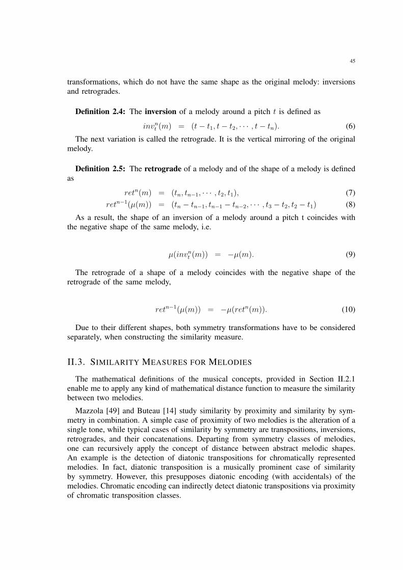
45

transformations, which do not have the same shape as the original melody: inversionsand retrogrades.

Definition 2.4: The inversion of a melody around a pitch t is defined as

invnt (m) = (t− t1, t− t2, · · · , t− tn). (6)

The next variation is called the retrograde. It is the vertical mirroring of the originalmelody.

Definition 2.5: The retrograde of a melody and of the shape of a melody is definedas

retn(m) = (tn, tn−1, · · · , t2, t1), (7)retn−1(µ(m)) = (tn − tn−1, tn−1 − tn−2, · · · , t3 − t2, t2 − t1) (8)

As a result, the shape of an inversion of a melody around a pitch t coincides withthe negative shape of the same melody, i.e.

µ(invnt (m)) = −µ(m). (9)

The retrograde of a shape of a melody coincides with the negative shape of theretrograde of the same melody,

retn−1(µ(m)) = −µ(retn(m)). (10)

Due to their different shapes, both symmetry transformations have to be consideredseparately, when constructing the similarity measure.

II.3. SIMILARITY MEASURES FOR MELODIES

The mathematical definitions of the musical concepts, provided in Section II.2.1enable me to apply any kind of mathematical distance function to measure the similaritybetween two melodies.

Mazzola [49] and Buteau [14] study similarity by proximity and similarity by sym-metry in combination. A simple case of proximity of two melodies is the alteration of asingle tone, while typical cases of similarity by symmetry are transpositions, inversions,retrogrades, and their concatenations. Departing from symmetry classes of melodies,one can recursively apply the concept of distance between abstract melodic shapes.An example is the detection of diatonic transpositions for chromatically representedmelodies. In fact, diatonic transposition is a musically prominent case of similarityby symmetry. However, this presupposes diatonic encoding (with accidentals) of themelodies. Chromatic encoding can indirectly detect diatonic transpositions via proximityof chromatic transposition classes.

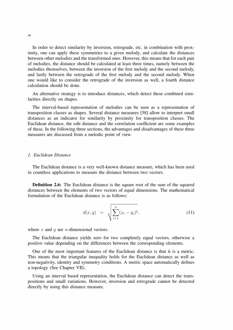
46

In order to detect similarity by inversion, retrograde, etc. in combination with prox-imity, one can apply these symmetries to a given melody, and calculate the distancesbetween other melodies and the transformed ones. However, this means that for each pairof melodies, the distance should be calculated at least three times, namely between themelodies themselves, between the inversion of the first melody and the second melody,and lastly between the retrograde of the first melody and the second melody. Whenone would like to consider the retrograde of the inversion as well, a fourth distancecalculation should be done.

An alternative strategy is to introduce distances, which detect these combined simi-larities directly on shapes.

The interval-based representation of melodies can be seen as a representation oftransposition classes as shapes. Several distance measures [58] allow to interpret smalldistances as an indicator for similarity by proximity for transposition classes. TheEuclidean distance, the edit distance and the correlation coefficient are some examplesof these. In the following three sections, the advantages and disadvantages of these threemeasures are discussed from a melodic point of view.

1. Euclidean Distance

The Euclidean distance is a very well-known distance measure, which has been usedin countless applications to measure the distance between two vectors.

Definition 2.6: The Euclidean distance is the square root of the sum of the squareddistances between the elements of two vectors of equal dimensions. The mathematicalformulation of the Euclidean distance is as follows:

d(x, y) =

√√√√ n∑i=1

(xi − yi)2, (11)

where x and y are n-dimensional vectors.

The Euclidean distance yields zero for two completely equal vectors, otherwise apositive value depending on the differences between the corresponding elements.

One of the most important features of the Euclidean distance is that it is a metric.This means that the triangular inequality holds for the Euclidean distance as well asnon-negativity, identity and symmetry conditions. A metric space automatically definesa topology (See Chapter VII).

Using an interval based representation, the Euclidean distance can detect the trans-positions and small variations. However, inversion and retrograde cannot be detecteddirectly by using this distance measure.

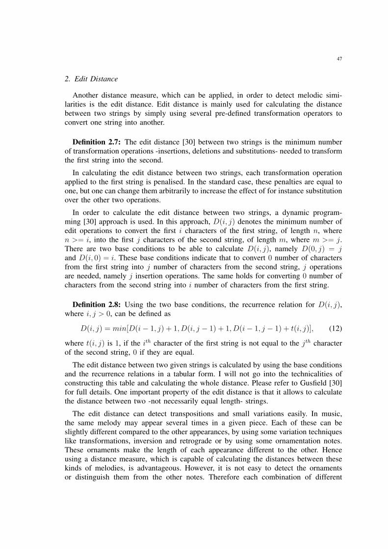
47

2. Edit Distance

Another distance measure, which can be applied, in order to detect melodic simi-larities is the edit distance. Edit distance is mainly used for calculating the distancebetween two strings by simply using several pre-defined transformation operators toconvert one string into another.

Definition 2.7: The edit distance [30] between two strings is the minimum numberof transformation operations -insertions, deletions and substitutions- needed to transformthe first string into the second.

In calculating the edit distance between two strings, each transformation operationapplied to the first string is penalised. In the standard case, these penalties are equal toone, but one can change them arbitrarily to increase the effect of for instance substitutionover the other two operations.

In order to calculate the edit distance between two strings, a dynamic program-ming [30] approach is used. In this approach, D(i, j) denotes the minimum number ofedit operations to convert the first i characters of the first string, of length n, wheren >= i, into the first j characters of the second string, of length m, where m >= j.There are two base conditions to be able to calculate D(i, j), namely D(0, j) = jand D(i, 0) = i. These base conditions indicate that to convert 0 number of charactersfrom the first string into j number of characters from the second string, j operationsare needed, namely j insertion operations. The same holds for converting 0 number ofcharacters from the second string into i number of characters from the first string.

Definition 2.8: Using the two base conditions, the recurrence relation for D(i, j),where i, j > 0, can be defined as

D(i, j) = min[D(i− 1, j) + 1, D(i, j − 1) + 1, D(i− 1, j − 1) + t(i, j)], (12)

where t(i, j) is 1, if the ith character of the first string is not equal to the jth characterof the second string, 0 if they are equal.

The edit distance between two given strings is calculated by using the base conditionsand the recurrence relations in a tabular form. I will not go into the technicalities ofconstructing this table and calculating the whole distance. Please refer to Gusfield [30]for full details. One important property of the edit distance is that it allows to calculatethe distance between two -not necessarily equal length- strings.

The edit distance can detect transpositions and small variations easily. In music,the same melody may appear several times in a given piece. Each of these can beslightly different compared to the other appearances, by using some variation techniqueslike transformations, inversion and retrograde or by using some ornamentation notes.These ornaments make the length of each appearance different to the other. Henceusing a distance measure, which is capable of calculating the distances between thesekinds of melodies, is advantageous. However, it is not easy to detect the ornamentsor distinguish them from the other notes. Therefore each combination of different

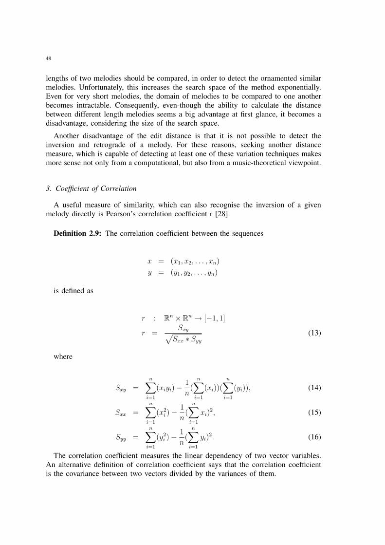
48

lengths of two melodies should be compared, in order to detect the ornamented similarmelodies. Unfortunately, this increases the search space of the method exponentially.Even for very short melodies, the domain of melodies to be compared to one anotherbecomes intractable. Consequently, even-though the ability to calculate the distancebetween different length melodies seems a big advantage at first glance, it becomes adisadvantage, considering the size of the search space.

Another disadvantage of the edit distance is that it is not possible to detect theinversion and retrograde of a melody. For these reasons, seeking another distancemeasure, which is capable of detecting at least one of these variation techniques makesmore sense not only from a computational, but also from a music-theoretical viewpoint.

3. Coefficient of Correlation

A useful measure of similarity, which can also recognise the inversion of a givenmelody directly is Pearson’s correlation coefficient r [28].

Definition 2.9: The correlation coefficient between the sequences

x = (x1, x2, . . . , xn)

y = (y1, y2, . . . , yn)

is defined as

r : Rn × Rn → [−1, 1]

r =Sxy√

Sxx ∗ Syy

(13)

where

Sxy =n∑

i=1

(xiyi)−1

n(

n∑i=1

(xi))(n∑

i=1

(yi)), (14)

Sxx =n∑

i=1

(x2i )−

1

n(

n∑i=1

xi)2, (15)

Syy =n∑

i=1

(y2i )−

1

n(

n∑i=1

yi)2. (16)

The correlation coefficient measures the linear dependency of two vector variables.An alternative definition of correlation coefficient says that the correlation coefficientis the covariance between two vectors divided by the variances of them.

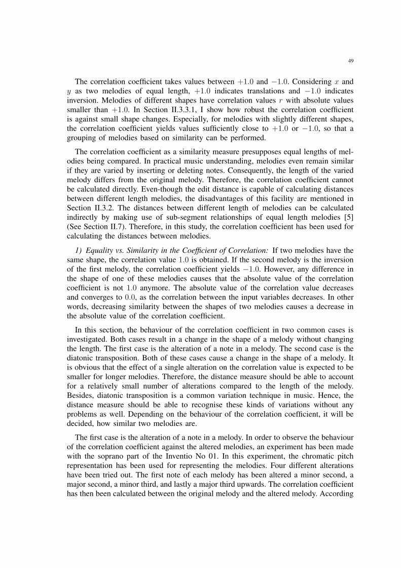
49

The correlation coefficient takes values between +1.0 and −1.0. Considering x andy as two melodies of equal length, +1.0 indicates translations and −1.0 indicatesinversion. Melodies of different shapes have correlation values r with absolute valuessmaller than +1.0. In Section II.3.3.1, I show how robust the correlation coefficientis against small shape changes. Especially, for melodies with slightly different shapes,the correlation coefficient yields values sufficiently close to +1.0 or −1.0, so that agrouping of melodies based on similarity can be performed.

The correlation coefficient as a similarity measure presupposes equal lengths of mel-odies being compared. In practical music understanding, melodies even remain similarif they are varied by inserting or deleting notes. Consequently, the length of the variedmelody differs from the original melody. Therefore, the correlation coefficient cannotbe calculated directly. Even-though the edit distance is capable of calculating distancesbetween different length melodies, the disadvantages of this facility are mentioned inSection II.3.2. The distances between different length of melodies can be calculatedindirectly by making use of sub-segment relationships of equal length melodies [5](See Section II.7). Therefore, in this study, the correlation coefficient has been used forcalculating the distances between melodies.

1) Equality vs. Similarity in the Coefficient of Correlation: If two melodies have thesame shape, the correlation value 1.0 is obtained. If the second melody is the inversionof the first melody, the correlation coefficient yields −1.0. However, any difference inthe shape of one of these melodies causes that the absolute value of the correlationcoefficient is not 1.0 anymore. The absolute value of the correlation value decreasesand converges to 0.0, as the correlation between the input variables decreases. In otherwords, decreasing similarity between the shapes of two melodies causes a decrease inthe absolute value of the correlation coefficient.

In this section, the behaviour of the correlation coefficient in two common cases isinvestigated. Both cases result in a change in the shape of a melody without changingthe length. The first case is the alteration of a note in a melody. The second case is thediatonic transposition. Both of these cases cause a change in the shape of a melody. Itis obvious that the effect of a single alteration on the correlation value is expected to besmaller for longer melodies. Therefore, the distance measure should be able to accountfor a relatively small number of alterations compared to the length of the melody.Besides, diatonic transposition is a common variation technique in music. Hence, thedistance measure should be able to recognise these kinds of variations without anyproblems as well. Depending on the behaviour of the correlation coefficient, it will bedecided, how similar two melodies are.

The first case is the alteration of a note in a melody. In order to observe the behaviourof the correlation coefficient against the altered melodies, an experiment has been madewith the soprano part of the Inventio No 01. In this experiment, the chromatic pitchrepresentation has been used for representing the melodies. Four different alterationshave been tried out. The first note of each melody has been altered a minor second, amajor second, a minor third, and lastly a major third upwards. The correlation coefficienthas then been calculated between the original melody and the altered melody. According

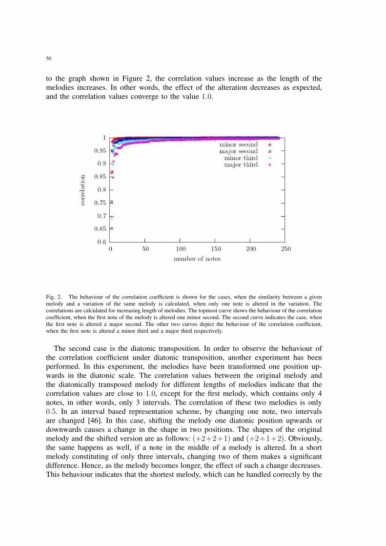
50

to the graph shown in Figure 2, the correlation values increase as the length of themelodies increases. In other words, the effect of the alteration decreases as expected,and the correlation values converge to the value 1.0.

Fig. 2. The behaviour of the correlation coefficient is shown for the cases, when the similarity between a givenmelody and a variation of the same melody is calculated, when only one note is altered in the variation. Thecorrelations are calculated for increasing length of melodies. The topmost curve shows the behaviour of the correlationcoefficient, when the first note of the melody is altered one minor second. The second curve indicates the case, whenthe first note is altered a major second. The other two curves depict the behaviour of the correlation coefficient,when the first note is altered a minor third and a major third respectively.

The second case is the diatonic transposition. In order to observe the behaviour ofthe correlation coefficient under diatonic transposition, another experiment has beenperformed. In this experiment, the melodies have been transformed one position up-wards in the diatonic scale. The correlation values between the original melody andthe diatonically transposed melody for different lengths of melodies indicate that thecorrelation values are close to 1.0, except for the first melody, which contains only 4notes, in other words, only 3 intervals. The correlation of these two melodies is only0.5. In an interval based representation scheme, by changing one note, two intervalsare changed [46]. In this case, shifting the melody one diatonic position upwards ordownwards causes a change in the shape in two positions. The shapes of the originalmelody and the shifted version are as follows: (+2+2+1) and (+2+1+2). Obviously,the same happens as well, if a note in the middle of a melody is altered. In a shortmelody constituting of only three intervals, changing two of them makes a significantdifference. Hence, as the melody becomes longer, the effect of such a change decreases.This behaviour indicates that the shortest melody, which can be handled correctly by the

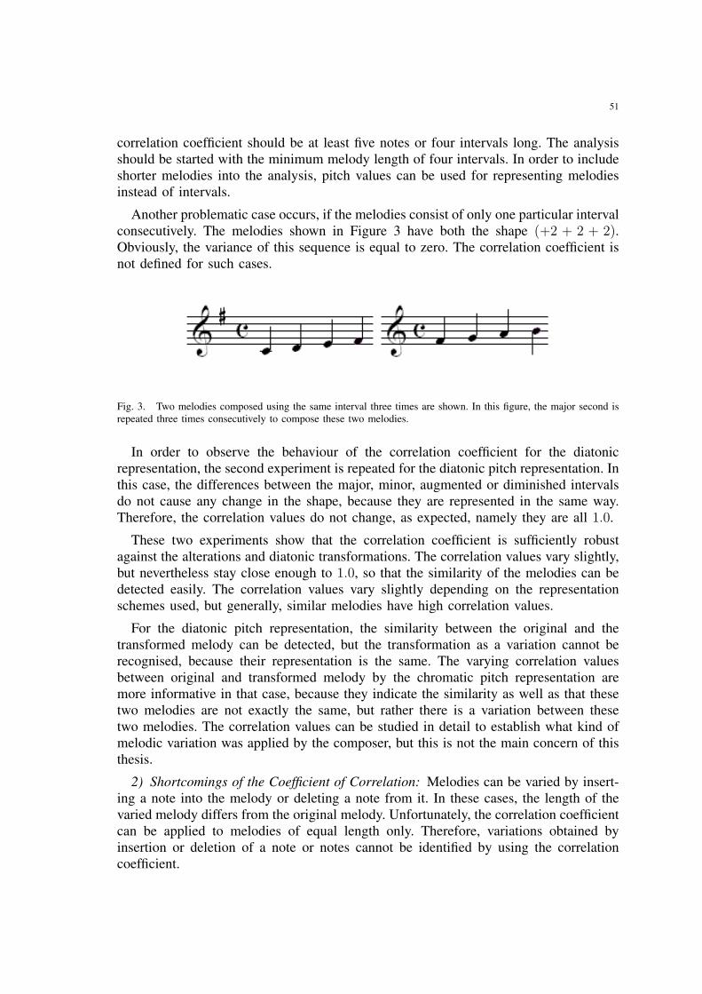
51

correlation coefficient should be at least five notes or four intervals long. The analysisshould be started with the minimum melody length of four intervals. In order to includeshorter melodies into the analysis, pitch values can be used for representing melodiesinstead of intervals.

Another problematic case occurs, if the melodies consist of only one particular intervalconsecutively. The melodies shown in Figure 3 have both the shape (+2 + 2 + 2).Obviously, the variance of this sequence is equal to zero. The correlation coefficient isnot defined for such cases.

Fig. 3. Two melodies composed using the same interval three times are shown. In this figure, the major second isrepeated three times consecutively to compose these two melodies.

In order to observe the behaviour of the correlation coefficient for the diatonicrepresentation, the second experiment is repeated for the diatonic pitch representation. Inthis case, the differences between the major, minor, augmented or diminished intervalsdo not cause any change in the shape, because they are represented in the same way.Therefore, the correlation values do not change, as expected, namely they are all 1.0.

These two experiments show that the correlation coefficient is sufficiently robustagainst the alterations and diatonic transformations. The correlation values vary slightly,but nevertheless stay close enough to 1.0, so that the similarity of the melodies can bedetected easily. The correlation values vary slightly depending on the representationschemes used, but generally, similar melodies have high correlation values.

For the diatonic pitch representation, the similarity between the original and thetransformed melody can be detected, but the transformation as a variation cannot berecognised, because their representation is the same. The varying correlation valuesbetween original and transformed melody by the chromatic pitch representation aremore informative in that case, because they indicate the similarity as well as that thesetwo melodies are not exactly the same, but rather there is a variation between thesetwo melodies. The correlation values can be studied in detail to establish what kind ofmelodic variation was applied by the composer, but this is not the main concern of thisthesis.

2) Shortcomings of the Coefficient of Correlation: Melodies can be varied by insert-ing a note into the melody or deleting a note from it. In these cases, the length of thevaried melody differs from the original melody. Unfortunately, the correlation coefficientcan be applied to melodies of equal length only. Therefore, variations obtained byinsertion or deletion of a note or notes cannot be identified by using the correlationcoefficient.

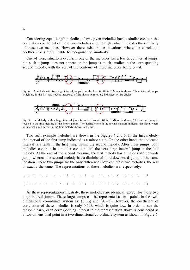
52

Considering equal length melodies, if two given melodies have a similar contour, thecorrelation coefficient of those two melodies is quite high, which indicates the similarityof these two melodies. However there exists some situations, where the correlationcoefficient is simply unable to recognise the similarity.

One of these situations occurs, if one of the melodies has a few large interval jumps,but such a jump does not appear or the jump is much smaller in the correspondingsecond melody, with the rest of the contours of these melodies being equal.

Fig. 4. A melody with two large interval jumps from the Inventio 09 in F Minor is shown. These interval jumps,which are in the first and second measures of the shown phrase, are indicated by the circles.

Fig. 5. A Melody with a large interval jump from the Inventio 09 in F Minor is shown. This interval jump islocated in the first measure of the shown phrase. The dashed circle in the second measure indicates the place, wherean interval jump occurs in the first melody shown in Figure 4.

Two such example melodies are shown in the Figures 4 and 5. In the first melody,the interval of the first jump indicated is a minor sixth. On the other hand, the indicatedinterval is a tenth in the first jump within the second melody. After those jumps, bothmelodies continue in a similar contour until the next large interval jump in the firstmelody. At the end of the second measure, the first melody has a major sixth upwardsjump, whereas the second melody has a diminished third downwards jump at the samelocation. These two jumps are the only differences between these two melodies, the restis exactly the same. The representations of these melodies are respectively:

(-2 -2 -1 1 -3 8 -1 -2 -1 1 -3 9 1 2 1 2 -3 -3 -3 -1)

(-2 -2 -1 1 -3 15 -1 -2 -1 1 -3 -3 1 2 1 2 -3 -3 -3 -1)

As these representations illustrate, these melodies are identical, except for those twolarge interval jumps. These large jumps can be represented as two points in the two-dimensional co-ordinate system as: (8, 15) and (9,−3). However, the coefficient ofcorrelation of these melodies is only 0.643, which is quite low. In order to see thereason clearly, each corresponding interval in the representation above is considered asa two-dimensional point in a two-dimensional co-ordinate system as shown in Figure 6.

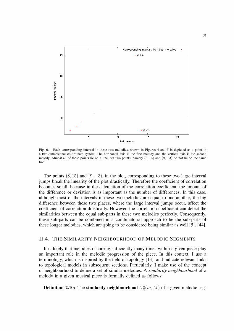
53

Fig. 6. Each corresponding interval in these two melodies, shown in Figures 4 and 5 is depicted as a point ina two-dimensional co-ordinate system. The horizontal axis is the first melody and the vertical axis is the secondmelody. Almost all of these points lie on a line, but two points, namely (8, 15) and (9,−3) do not lie on the sameline.

The points (8, 15) and (9,−3), in the plot, corresponding to these two large intervaljumps break the linearity of the plot drastically. Therefore the coefficient of correlationbecomes small, because in the calculation of the correlation coefficient, the amount ofthe difference or deviation is as important as the number of differences. In this case,although most of the intervals in these two melodies are equal to one another, the bigdifference between these two places, where the large interval jumps occur, affect thecoefficient of correlation drastically. However, the correlation coefficient can detect thesimilarities between the equal sub-parts in these two melodies perfectly. Consequently,these sub-parts can be combined in a combinatorial approach to be the sub-parts ofthese longer melodies, which are going to be considered being similar as well [5]. [44].

II.4. THE SIMILARITY NEIGHBOURHOOD OF MELODIC SEGMENTS

It is likely that melodies occurring sufficiently many times within a given piece playan important role in the melodic progression of the piece. In this context, I use aterminology, which is inspired by the field of topology [13], and indicate relevant linksto topological models in subsequent sections. Particularly, I make use of the conceptof neighbourhood to define a set of similar melodies. A similarity neighbourhood of amelody in a given musical piece is formally defined as follows:

Definition 2.10: The similarity neighbourhood UnR(m, M) of a given melodic seg-

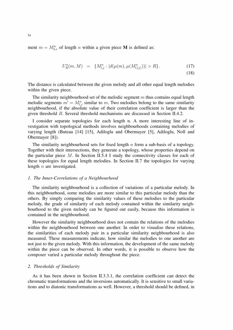
54

ment m = Mnk,i of length n within a given piece M is defined as:

UnR(m, M) = {Mn

l,j : |d(µ(m), µ(Mnl,(j)))| > R}. (17)

(18)

The distance is calculated between the given melody and all other equal length melodieswithin the given piece.

The similarity neighbourhood set of the melodic segment m thus contains equal lengthmelodic segments m′ = Mn

l,j similar to m. Two melodies belong to the same similarityneighbourhood, if the absolute value of their correlation coefficient is larger than thegiven threshold R. Several threshold mechanisms are discussed in Section II.4.2.

I consider separate topologies for each length n. A more interesting line of in-vestigation with topological methods involves neighbourhoods containing melodies ofvarying length (Buteau [14] [15], Adiloglu and Obermayer [5], Adiloglu, Noll andObermayer [8]).

The similarity neighbourhood sets for fixed length n form a sub-basis of a topology.Together with their intersections, they generate a topology, whose properties depend onthe particular piece M . In Section II.5.4 I study the connectivity classes for each ofthese topologies for equal length melodies. In Section II.7 the topologies for varyinglength n are investigated.

1. The Inner-Correlations of a Neighbourhood

The similarity neighbourhood is a collection of variations of a particular melody. Inthis neighbourhood, some melodies are more similar to this particular melody than theothers. By simply comparing the similarity values of these melodies to the particularmelody, the grade of similarity of each melody contained within the similarity neigh-bourhood to the given melody can be figured out easily, because this information iscontained in the neighbourhood.

However the similarity neighbourhood does not contain the relations of the melodieswithin the neighbourhood between one another. In order to visualise these relations,the similarities of each melody pair in a particular similarity neighbourhood is alsomeasured. These measurements indicate, how similar the melodies to one another arenot just to the given melody. With this information, the development of the same melodywithin the piece can be observed. In other words, it is possible to observe how thecomposer varied a particular melody throughout the piece.

2. Thresholds of Similarity

As it has been shown in Section II.3.3.1, the correlation coefficient can detect thechromatic transformations and the inversions automatically. It is sensitive to small varia-tions and to diatonic transformations as well. However, a threshold should be defined, in

55

order to distinguish these variations and transformations from other differences betweendissimilar melodies.

In this study, I defined two types of thresholds. The first type is called the normalthresholds. These thresholds simply use the length of the given melody and the lengthof the piece (, which is constant, of course). The threshold decreases as the lengthof melodies increase, in order to be able to account for the variation possibilities oflonger melodies. The second type of the thresholds incorporate the calculated distancevalues for a similarity neighbourhood to adapt the threshold to these distance valuesheuristically. Therefore these distances are called the heuristic distances.

1) Normal Thresholds: The first thresholds make use of the ratio of the length ofthe given melody to the length of the piece, where the given melody is in.

Definition 2.11: The similarity threshold of a given melody m of length n withina given piece M of length N is defined as:

R = 1− c1n

Nwhere c1 is a constant. (19)

Definition 2.12: The similarity threshold of a given melody m of length n withina given piece M of length N is defined as:

R = 1− c1

√n

Nwhere c1 is a constant. (20)

The next threshold of the similarity depends only on the length of the melody. Thereason, why only the length of the melody is taken into account is that the ratio betweenthe length of the melody and the length of the piece plays not an important role in thevariations of the melody. This ratio is only important to decide how long a melody canbe in a particular piece. How far a melody can be varied is mostly dependent only onthe length of the melody itself.

Definition 2.13: The similarity threshold depending only on the two given melodiesof length n is defined as:

R = 21

nc1 −1, where c1 is a constant. (21)

This threshold R depends on the length of the melody. As the melodies become larger,the possibilities to vary the melody become larger as well. Considering this fact, thethreshold starts with the value 1.0 for the melody of length 0 and decreases exponentiallyas the length of the melody increases. The threshold increases, when the constant c1

56

Fig. 7. The behaviour of the similarity neighbourhood threshold depending on the constant c1 is shown. Thesimilarity threshold decreases as the constant c1 increases.

is decreased. The behaviour of the similarity threshold looks like in Figure 7. In thisfigure, three curves are shown for three different values of the constant c1.

In the bottom-most curve, the constant c1 vanishes, and the length of the melodyaffects the threshold alone. In this case, the thresholds decrease very quickly, so thatit is quite small even for relatively short melodies. As the melodies get longer, thethreshold converges to 0.5. As the constant c1 becomes smaller, the threshold valuesdecrease not so quickly. Especially for short melodies, the threshold values become quitehigh. However, they still converge to 0.5 for the longer melodies, it takes more timethough. Therefore the short melodies can be detected more precisely, without loosing thelong melodies. Consequently, among the normal thresholds, this last threshold reflectsthe music-theoretical behaviour the closest. Therefore, I used this threshold in myexperiments.

2) Heuristic Thresholds: The threshold mechanism that I introduced in the previoussection considers only the length of the melodies. The threshold decreases as thelength of the melody increases. The intuitive reason, why the threshold decreases isthat there are more possibilities to make variations on the melodies, if the melodybecomes longer. The results obtained by using such a threshold supports this intuition(See Chapters IV, V and VI).

Another intuitive fact, which could affect the threshold mechanism in a positive wayis that similar melodies have high similarity values, and dissimilar melodies have lowsimilarity values. Departing from this idea, if the similarity values are sorted, a gap

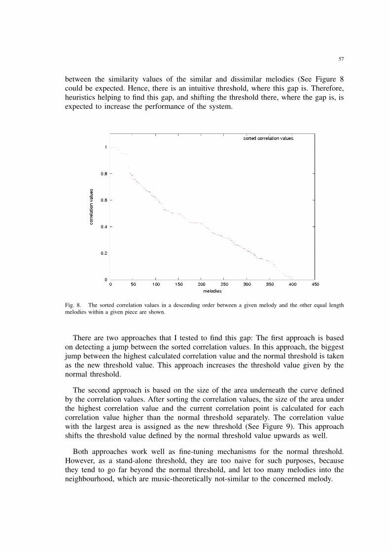
57

between the similarity values of the similar and dissimilar melodies (See Figure 8could be expected. Hence, there is an intuitive threshold, where this gap is. Therefore,heuristics helping to find this gap, and shifting the threshold there, where the gap is, isexpected to increase the performance of the system.

Fig. 8. The sorted correlation values in a descending order between a given melody and the other equal lengthmelodies within a given piece are shown.

There are two approaches that I tested to find this gap: The first approach is basedon detecting a jump between the sorted correlation values. In this approach, the biggestjump between the highest calculated correlation value and the normal threshold is takenas the new threshold value. This approach increases the threshold value given by thenormal threshold.

The second approach is based on the size of the area underneath the curve definedby the correlation values. After sorting the correlation values, the size of the area underthe highest correlation value and the current correlation point is calculated for eachcorrelation value higher than the normal threshold separately. The correlation valuewith the largest area is assigned as the new threshold (See Figure 9). This approachshifts the threshold value defined by the normal threshold value upwards as well.

Both approaches work well as fine-tuning mechanisms for the normal threshold.However, as a stand-alone threshold, they are too naive for such purposes, becausethey tend to go far beyond the normal threshold, and let too many melodies into theneighbourhood, which are music-theoretically not-similar to the concerned melody.

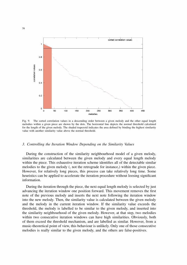
58

Fig. 9. The sorted correlation values in a descending order between a given melody and the other equal lengthmelodies within a given piece are shown by the dots. The horizontal line depicts the normal threshold calculatedfor the length of the given melody. The shaded trapezoid indicates the area defined by binding the highest similarityvalue with another similarity value above the normal threshold.

3. Controlling the Iteration Window Depending on the Similarity Values

During the construction of the similarity neighbourhood model of a given melody,similarities are calculated between the given melody and every equal length melodywithin the piece. This exhaustive iteration scheme identifies all of the detectable similarmelodies to the given melody (, not the retrograde for instance,) within the given piece.However, for relatively long pieces, this process can take relatively long time. Someheuristics can be applied to accelerate the iteration procedure without loosing significantinformation.

During the iteration through the piece, the next equal length melody is selected by justadvancing the iteration window one position forward. This movement removes the firstnote of the previous melody and inserts the next note following the iteration windowinto the new melody. Then, the similarity value is calculated between the given melodyand the melody in the current iteration window. If the similarity value exceeds thethreshold, the melody is labelled to be similar to the given melody, and inserted intothe similarity neighbourhood of the given melody. However, at that step, two melodieswithin two consecutive iteration windows can have high similarities. Obviously, bothof them exceed the threshold mechanism, and are labelled as similar. However, from amusic-theoretical point of view, this behaviour is unlikely. Only one of those consecutivemelodies is really similar to the given melody, and the others are false-positives.

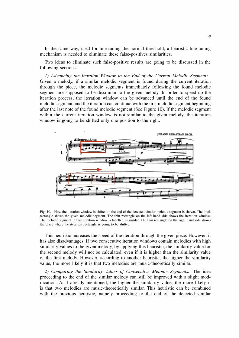
59

In the same way, used for fine-tuning the normal threshold, a heuristic fine-tuningmechanism is needed to eliminate these false-positives similarities.

Two ideas to eliminate such false-positive results are going to be discussed in thefollowing sections.

1) Advancing the Iteration Window to the End of the Current Melodic Segment:Given a melody, if a similar melodic segment is found during the current iterationthrough the piece, the melodic segments immediately following the found melodicsegment are supposed to be dissimilar to the given melody. In order to speed up theiteration process, the iteration window can be advanced until the end of the foundmelodic segment, and the iteration can continue with the first melodic segment beginningafter the last note of the found melodic segment (See Figure 10). If the melodic segmentwithin the current iteration window is not similar to the given melody, the iterationwindow is going to be shifted only one position to the right.

Fig. 10. How the iteration window is shifted to the end of the detected similar melodic segment is shown. The thickrectangle shows the given melodic segment. The thin rectangle on the left hand side shows the iteration window.The melodic segment in this iteration window is labelled as similar. The thin rectangle on the right hand side showsthe place where the iteration rectangle is going to be shifted.

This heuristic increases the speed of the iteration through the given piece. However, ithas also disadvantages. If two consecutive iteration windows contain melodies with highsimilarity values to the given melody, by applying this heuristic, the similarity value forthe second melody will not be calculated, even if it is higher than the similarity valueof the first melody. However, according to another heuristic, the higher the similarityvalue, the more likely it is that two melodies are music-theoretically similar.

2) Comparing the Similarity Values of Consecutive Melodic Segments: The ideaproceeding to the end of the similar melody can still be improved with a slight mod-ification. As I already mentioned, the higher the similarity value, the more likely itis that two melodies are music-theoretically similar. This heuristic can be combinedwith the previous heuristic, namely proceeding to the end of the detected similar

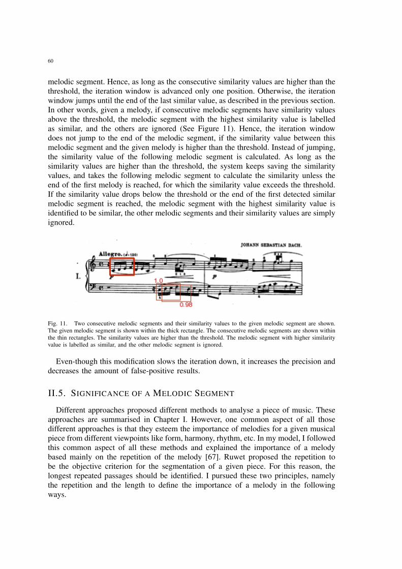
60

melodic segment. Hence, as long as the consecutive similarity values are higher than thethreshold, the iteration window is advanced only one position. Otherwise, the iterationwindow jumps until the end of the last similar value, as described in the previous section.In other words, given a melody, if consecutive melodic segments have similarity valuesabove the threshold, the melodic segment with the highest similarity value is labelledas similar, and the others are ignored (See Figure 11). Hence, the iteration windowdoes not jump to the end of the melodic segment, if the similarity value between thismelodic segment and the given melody is higher than the threshold. Instead of jumping,the similarity value of the following melodic segment is calculated. As long as thesimilarity values are higher than the threshold, the system keeps saving the similarityvalues, and takes the following melodic segment to calculate the similarity unless theend of the first melody is reached, for which the similarity value exceeds the threshold.If the similarity value drops below the threshold or the end of the first detected similarmelodic segment is reached, the melodic segment with the highest similarity value isidentified to be similar, the other melodic segments and their similarity values are simplyignored.

Fig. 11. Two consecutive melodic segments and their similarity values to the given melodic segment are shown.The given melodic segment is shown within the thick rectangle. The consecutive melodic segments are shown withinthe thin rectangles. The similarity values are higher than the threshold. The melodic segment with higher similarityvalue is labelled as similar, and the other melodic segment is ignored.

Even-though this modification slows the iteration down, it increases the precision anddecreases the amount of false-positive results.

II.5. SIGNIFICANCE OF A MELODIC SEGMENT

Different approaches proposed different methods to analyse a piece of music. Theseapproaches are summarised in Chapter I. However, one common aspect of all thosedifferent approaches is that they esteem the importance of melodies for a given musicalpiece from different viewpoints like form, harmony, rhythm, etc. In my model, I followedthis common aspect of all these methods and explained the importance of a melodybased mainly on the repetition of the melody [67]. Ruwet proposed the repetition tobe the objective criterion for the segmentation of a given piece. For this reason, thelongest repeated passages should be identified. I pursued these two principles, namelythe repetition and the length to define the importance of a melody in the followingways.

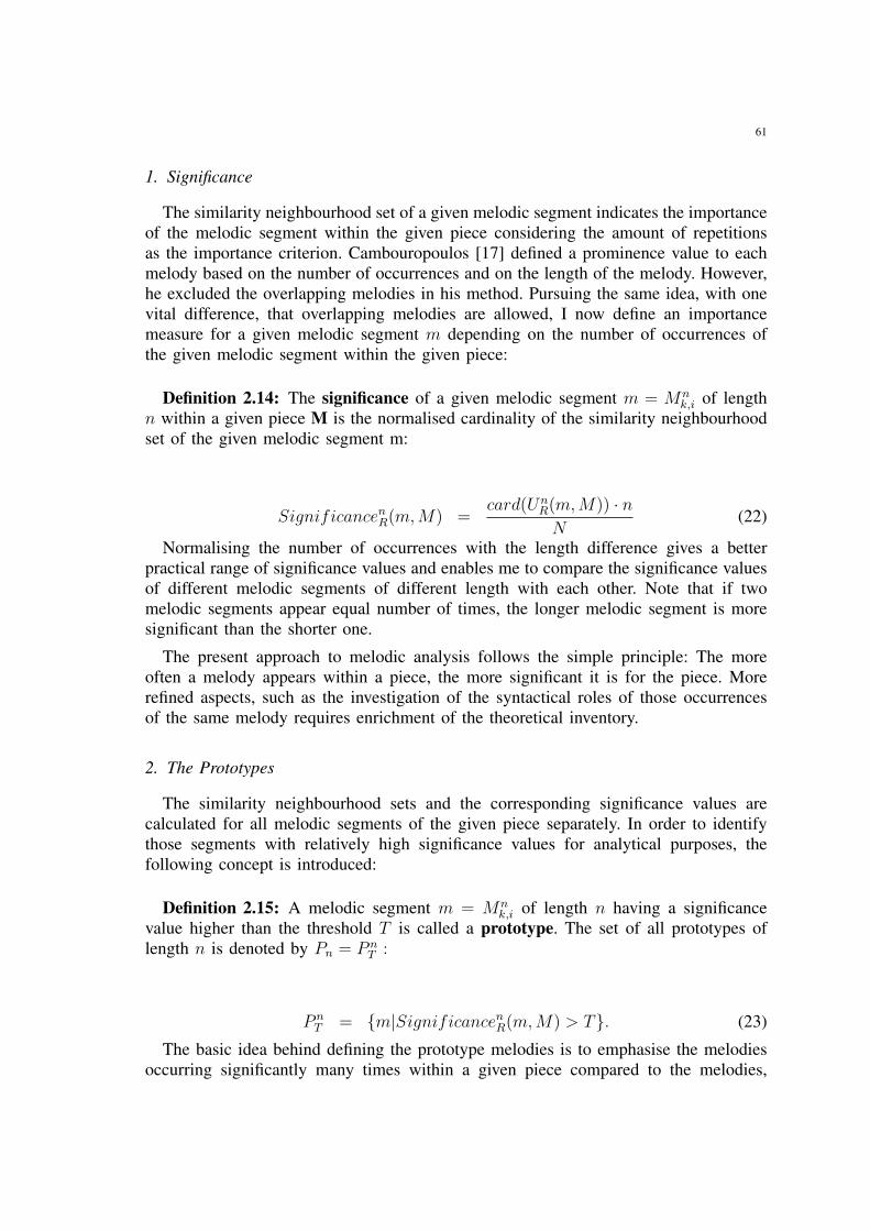
61

1. Significance

The similarity neighbourhood set of a given melodic segment indicates the importanceof the melodic segment within the given piece considering the amount of repetitionsas the importance criterion. Cambouropoulos [17] defined a prominence value to eachmelody based on the number of occurrences and on the length of the melody. However,he excluded the overlapping melodies in his method. Pursuing the same idea, with onevital difference, that overlapping melodies are allowed, I now define an importancemeasure for a given melodic segment m depending on the number of occurrences ofthe given melodic segment within the given piece:

Definition 2.14: The significance of a given melodic segment m = Mnk,i of length

n within a given piece M is the normalised cardinality of the similarity neighbourhoodset of the given melodic segment m:

SignificancenR(m, M) =

card(UnR(m, M)) · n

N(22)

Normalising the number of occurrences with the length difference gives a betterpractical range of significance values and enables me to compare the significance valuesof different melodic segments of different length with each other. Note that if twomelodic segments appear equal number of times, the longer melodic segment is moresignificant than the shorter one.

The present approach to melodic analysis follows the simple principle: The moreoften a melody appears within a piece, the more significant it is for the piece. Morerefined aspects, such as the investigation of the syntactical roles of those occurrencesof the same melody requires enrichment of the theoretical inventory.

2. The Prototypes

The similarity neighbourhood sets and the corresponding significance values arecalculated for all melodic segments of the given piece separately. In order to identifythose segments with relatively high significance values for analytical purposes, thefollowing concept is introduced:

Definition 2.15: A melodic segment m = Mnk,i of length n having a significance

value higher than the threshold T is called a prototype. The set of all prototypes oflength n is denoted by Pn = P n

T :

P nT = {m|Significancen

R(m, M) > T}. (23)

The basic idea behind defining the prototype melodies is to emphasise the melodiesoccurring significantly many times within a given piece compared to the melodies,

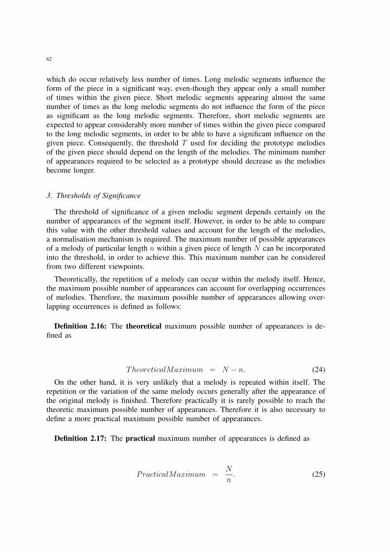
62

which do occur relatively less number of times. Long melodic segments influence theform of the piece in a significant way, even-though they appear only a small numberof times within the given piece. Short melodic segments appearing almost the samenumber of times as the long melodic segments do not influence the form of the pieceas significant as the long melodic segments. Therefore, short melodic segments areexpected to appear considerably more number of times within the given piece comparedto the long melodic segments, in order to be able to have a significant influence on thegiven piece. Consequently, the threshold T used for deciding the prototype melodiesof the given piece should depend on the length of the melodies. The minimum numberof appearances required to be selected as a prototype should decrease as the melodiesbecome longer.

3. Thresholds of Significance

The threshold of significance of a given melodic segment depends certainly on thenumber of appearances of the segment itself. However, in order to be able to comparethis value with the other threshold values and account for the length of the melodies,a normalisation mechanism is required. The maximum number of possible appearancesof a melody of particular length n within a given piece of length N can be incorporatedinto the threshold, in order to achieve this. This maximum number can be consideredfrom two different viewpoints.

Theoretically, the repetition of a melody can occur within the melody itself. Hence,the maximum possible number of appearances can account for overlapping occurrencesof melodies. Therefore, the maximum possible number of appearances allowing over-lapping occurrences is defined as follows:

Definition 2.16: The theoretical maximum possible number of appearances is de-fined as

TheoreticalMaximum = N − n. (24)

On the other hand, it is very unlikely that a melody is repeated within itself. Therepetition or the variation of the same melody occurs generally after the appearance ofthe original melody is finished. Therefore practically it is rarely possible to reach thetheoretic maximum possible number of appearances. Therefore it is also necessary todefine a more practical maximum possible number of appearances.

Definition 2.17: The practical maximum number of appearances is defined as

PracticalMaximum =N

n. (25)

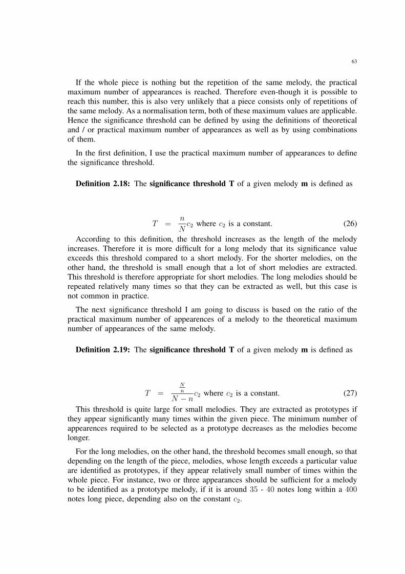
63

If the whole piece is nothing but the repetition of the same melody, the practicalmaximum number of appearances is reached. Therefore even-though it is possible toreach this number, this is also very unlikely that a piece consists only of repetitions ofthe same melody. As a normalisation term, both of these maximum values are applicable.Hence the significance threshold can be defined by using the definitions of theoreticaland / or practical maximum number of appearances as well as by using combinationsof them.

In the first definition, I use the practical maximum number of appearances to definethe significance threshold.

Definition 2.18: The significance threshold T of a given melody m is defined as

T =n

Nc2 where c2 is a constant. (26)

According to this definition, the threshold increases as the length of the melodyincreases. Therefore it is more difficult for a long melody that its significance valueexceeds this threshold compared to a short melody. For the shorter melodies, on theother hand, the threshold is small enough that a lot of short melodies are extracted.This threshold is therefore appropriate for short melodies. The long melodies should berepeated relatively many times so that they can be extracted as well, but this case isnot common in practice.

The next significance threshold I am going to discuss is based on the ratio of thepractical maximum number of appearences of a melody to the theoretical maximumnumber of appearances of the same melody.

Definition 2.19: The significance threshold T of a given melody m is defined as

T =Nn

N − nc2 where c2 is a constant. (27)

This threshold is quite large for small melodies. They are extracted as prototypes ifthey appear significantly many times within the given piece. The minimum number ofappearences required to be selected as a prototype decreases as the melodies becomelonger.

For the long melodies, on the other hand, the threshold becomes small enough, so thatdepending on the length of the piece, melodies, whose length exceeds a particular valueare identified as prototypes, if they appear relatively small number of times within thewhole piece. For instance, two or three appearances should be sufficient for a melodyto be identified as a prototype melody, if it is around 35 - 40 notes long within a 400notes long piece, depending also on the constant c2.

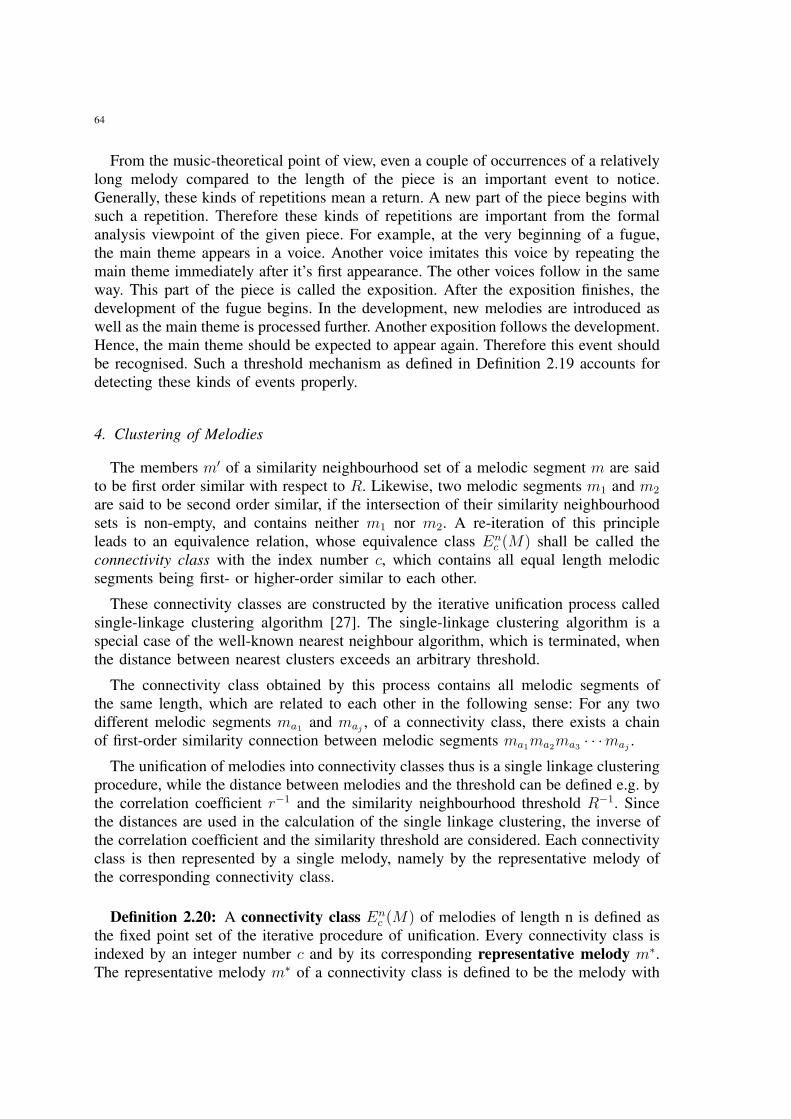
64

From the music-theoretical point of view, even a couple of occurrences of a relativelylong melody compared to the length of the piece is an important event to notice.Generally, these kinds of repetitions mean a return. A new part of the piece begins withsuch a repetition. Therefore these kinds of repetitions are important from the formalanalysis viewpoint of the given piece. For example, at the very beginning of a fugue,the main theme appears in a voice. Another voice imitates this voice by repeating themain theme immediately after it’s first appearance. The other voices follow in the sameway. This part of the piece is called the exposition. After the exposition finishes, thedevelopment of the fugue begins. In the development, new melodies are introduced aswell as the main theme is processed further. Another exposition follows the development.Hence, the main theme should be expected to appear again. Therefore this event shouldbe recognised. Such a threshold mechanism as defined in Definition 2.19 accounts fordetecting these kinds of events properly.

4. Clustering of Melodies

The members m′ of a similarity neighbourhood set of a melodic segment m are saidto be first order similar with respect to R. Likewise, two melodic segments m1 and m2

are said to be second order similar, if the intersection of their similarity neighbourhoodsets is non-empty, and contains neither m1 nor m2. A re-iteration of this principleleads to an equivalence relation, whose equivalence class En

c (M) shall be called theconnectivity class with the index number c, which contains all equal length melodicsegments being first- or higher-order similar to each other.

These connectivity classes are constructed by the iterative unification process calledsingle-linkage clustering algorithm [27]. The single-linkage clustering algorithm is aspecial case of the well-known nearest neighbour algorithm, which is terminated, whenthe distance between nearest clusters exceeds an arbitrary threshold.

The connectivity class obtained by this process contains all melodic segments ofthe same length, which are related to each other in the following sense: For any twodifferent melodic segments ma1 and maj

, of a connectivity class, there exists a chainof first-order similarity connection between melodic segments ma1ma2ma3 · · ·maj

.

The unification of melodies into connectivity classes thus is a single linkage clusteringprocedure, while the distance between melodies and the threshold can be defined e.g. bythe correlation coefficient r−1 and the similarity neighbourhood threshold R−1. Sincethe distances are used in the calculation of the single linkage clustering, the inverse ofthe correlation coefficient and the similarity threshold are considered. Each connectivityclass is then represented by a single melody, namely by the representative melody ofthe corresponding connectivity class.

Definition 2.20: A connectivity class Enc (M) of melodies of length n is defined as

the fixed point set of the iterative procedure of unification. Every connectivity class isindexed by an integer number c and by its corresponding representative melody m∗.The representative melody m∗ of a connectivity class is defined to be the melody with

65

the similarity neighbourhood set of largest cardinality. If there is more than one melodyhaving a similarity neighbourhood set of maximal cardinality, the melody appearing atfirst is chosen to be the representative melody of the corresponding connectivity class.

As special sub-sets of the connectivity classes, I also consider the prototypical con-nectivity classes, which have the property that second and higher order similarities areonly allowed for prototypes. In other words, prototypical connectivity classes containonly prototypes as well as first order similar melodies to them, and the similarityneighbourhoods of non-prototypical melodies are ignored. This does not only implythe ignorance of non-prototypical melodies but also of non-prototypical connections.The implemented algorithm produces the prototypical connectivity classes; dependingon the prototypicity threshold. If the significance threshold is set to zero, both conceptscoincide, i.e. the prototypical and the non-prototypical connectivity classes are the same.

Constructing the connectivity classes simplifies the control of the results, and indicatesthe second, third and higher order similarities of melodies in a better way.

A connectivity class with it’s representative melody gives an easy access to theotherwise large amount of results. Departing from each of these representatives, onemay navigate through the connectivity classes along first, second and higher ordersimilarities. Note that the connectivity classes are mutually disjoint:

Corollary 2.1: The intersection of any connectivity classes is the empty set.

II.6. THE PROMINENCE PROFILE

The prototypes identify the melodies that appear more than indicated by a particularthreshold value within the given piece. From this point of view, these melodies areconsidered to be important for the given piece. In order to give useful clues about thefurther analysis of the given piece, a new concept is defined, which accounts for theseimportant melodies separately for each length value. This new concept is called theprominence profile of the given piece. In this profile, the total amount of prototypes aswell as the connectivity classes are presented for each length of melodies separately.In the following, the total number of connectivity classes (i.e. the total number ofrepresentative melodies) of melodies of length n is denoted by Rep(n).

The connectivity classes with the largest number of prototype melodies are likelyto contain the most important melodies for a given piece. Correspondingly, if thereare many connectivity classes with comparatively few elements, one can deduce thatthe representative melodies of these connectivity classes are not as important as therepresentative melodies of the others with many melodies. Departing from this idea, amelodic profile of the given piece is obtained in terms of the connectivity classes. Thisnew concept is defined in the following:

Definition 2.21: The prominence profile of a given piece M is the average numberof prototype melodies within the connectivity classes for each length value, which isdefined as

66

Profile(M) = (card(P nmin

T )

Rep(nmin)nmin,

card(P nmin+1T )

Rep(nmin + 1)(nmin + 1), . . .). (28)

nmin is the length of the shortest melodic segments, which are considered in theanalysis of the piece. Each co-ordinate of this vector, corresponding to a particularlength value indicates the distribution of the prototypes among the connectivity classesfor this particular length. These values are multiplied by the corresponding length valuesof the melodies, in order to account for the importance of longer melodies. In otherwords, the prominence of the melodies of a particular length within the given piece isindicated by the co-ordinates of the prominence profile.

The similarity neighbourhood set of a prototype melody contains possibly melodies,which are not prototypes themselves. Therefore the total number of prototypes is notnecessarily equal to the total number of melodies identified to be similar. In orderto account for the total number of melodies identified to be similar to each other, asimilar prominence profile is calculated for the connectivity classes. After generatingthe connectivity classes, the prominence value of the classes are calculated individuallyfor each length value of the melodies. The second version of the prominence profileaccounts for the average number of melodies for each connectivity class.

Definition 2.22: The prominence profile of a given piece M is the average numberof melodies within connectivity classes for each length value, which is defined as

Profile(M) = (

∑Cnminc=1 (card(Enmin

c (M)))

Rep(nmin)nmin, (29)∑Cnmin+1

c=1 (card(Enmin+1c (M)))

Rep(nmin + 1)(nmin + 1),

. . .).

The prominence profile indicates in a practical way, which length of the connectivityclasses should be investigated in detail, in order to identify the most important melodiesof a given piece from a paradigmatic point of view. However, these values do notalways single out music-theoretically important melodies. Due to the averaging, theconnectivity classes with the largest number of melodies cannot be identified easily byusing the prominence profile, depending on the deviation from the averaged numberof melodies. Therefore the standard deviation from this mean value is calculated foreach connectivity class as well. On the one hand, if the deviation is relatively low,the distribution of the melodies among the connectivity classes is fairly equal. In otherwords, the connectivity classes contain roughly equal number of melodies. This meansthat none of the connectivity classes are more important than the others. On the otherhand, if the deviation is large, some of the connectivity classes contain comparativelymore melodies than the others. Hence, these connectivity classes deserve special interest.For this reason, the number of melodies contained in the biggest connectivity classes

67

of each particular length should also be considered. Therefore, weighted number ofmelodies contained in the biggest connectivity class is defined as a second alternativeto the first definition of the prominence profile as follows:

Definition 2.23: The prominence profile of a given piece M is the weighted numberof melodies within the biggest connectivity class for each length value, which is definedas

Profile(M) = (argmaxi(card(Enminc (M)))nmin, (30)

argmaxi(card(Enmin+1d (M))(nmin + 1),

. . .).

These alternative definitions together with the first definition of the prominence profileenable to identify the biggest connectivity classes, in turn the melodies with the mostnumber of similar melodies for each length.

II.7. SUB-SEGMENT RELATIONSHIPS OF MELODIES

The melodic structure of a given musical piece is a hierarchical organisation in thesense that larger structures are divided into smaller structures even in simple musicalpieces. Therefore, as a result of a music-theoretical analysis [65], a musical piece issegmented into smaller parts on different levels. In general, a musical piece can bedivided into periods, which are sub-divided into phrases, etc. Similarly, a relativelylong melody is divided into smaller melodies (See Definition 2.2), which appear ondifferent locations within the piece independent of their ambient melodies. A music-theoretically complete melodic analysis of a given piece explains how the melodicmaterial is introduced, and used throughout the given piece. Therefore, in order tobe able to account for the introduction and usage of the melodic material, the sub-segment relationships between melodies should be identified as well. The similarityneighbourhood model, defined so far, takes only similarities between equal lengthmelodies into account. Therefore the model can identify how the melodic materialis introduced. However, how the melodic material is used throughout the given piececannot be explained by the model.

In order to investigate, how the melodic material is used as well, the inheritance of themelodic features between melodies is defined. The inheritance of the similarity relationsbetween melodies accounts for the similarity of the sub-segments. The inheritanceproperty is used as a condition to introduce two additional neighbourhood sets, whichexplain the sub-segment relationships between melodies.

1. Inheritance Property

Intuitively speaking, the practice of passing on some properties or features is calledinheritance. In the mathematical music theory domain, the inheritance property accounts

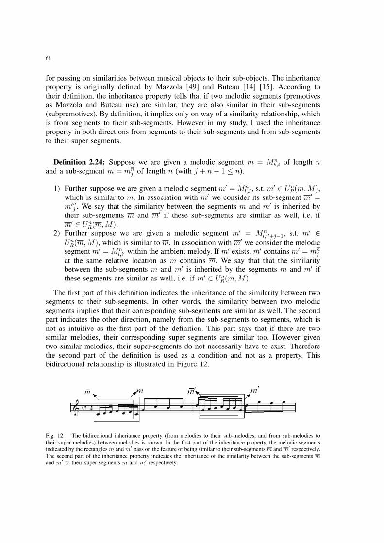
68

for passing on similarities between musical objects to their sub-objects. The inheritanceproperty is originally defined by Mazzola [49] and Buteau [14] [15]. According totheir definition, the inheritance property tells that if two melodic segments (premotivesas Mazzola and Buteau use) are similar, they are also similar in their sub-segments(subpremotives). By definition, it implies only on way of a similarity relationship, whichis from segments to their sub-segments. However in my study, I used the inheritanceproperty in both directions from segments to their sub-segments and from sub-segmentsto their super segments.

Definition 2.24: Suppose we are given a melodic segment m = Mnk,i of length n

and a sub-segment m = mnj of length n (with j + n− 1 ≤ n).

1) Further suppose we are given a melodic segment m′ = Mnl,i′ , s.t. m′ ∈ Un

R(m, M),which is similar to m. In association with m′ we consider its sub-segment m′ =m′n

j . We say that the similarity between the segments m and m′ is inherited bytheir sub-segments m and m′ if these sub-segments are similar as well, i.e. ifm′ ∈ Un

R(m,M).2) Further suppose we are given a melodic segment m′ = Mn

l,i′+j−1, s.t. m′ ∈Un

R(m, M), which is similar to m. In association with m′ we consider the melodicsegment m′ = Mn

l,i′ within the ambient melody. If m′ exists, m′ contains m′ = mnj

at the same relative location as m contains m. We say that that the similaritybetween the sub-segments m and m′ is inherited by the segments m and m′ ifthese segments are similar as well, i.e. if m′ ∈ Un

R(m, M).

The first part of this definition indicates the inheritance of the similarity between twosegments to their sub-segments. In other words, the similarity between two melodicsegments implies that their corresponding sub-segments are similar as well. The secondpart indicates the other direction, namely from the sub-segments to segments, which isnot as intuitive as the first part of the definition. This part says that if there are twosimilar melodies, their corresponding super-segments are similar too. However giventwo similar melodies, their super-segments do not necessarily have to exist. Thereforethe second part of the definition is used as a condition and not as a property. Thisbidirectional relationship is illustrated in Figure 12.

Fig. 12. The bidirectional inheritance property (from melodies to their sub-melodies, and from sub-melodies totheir super melodies) between melodies is shown. In the first part of the inheritance property, the melodic segmentsindicated by the rectangles m and m′ pass on the feature of being similar to their sub-segments m and m′ respectively.The second part of the inheritance property indicates the inheritance of the similarity between the sub-segments mand m′ to their super-segments m and m′ respectively.

69

2. The Presence Neighbourhood

Intuitively, the presence of a given melody within a given piece is the appearancesof the melody and of its similar melodies within the given piece. The given piece isthe ambient space containing the given melody. A melody defined as a segment of thegiven piece fulfils this condition (See Definition 2.2). The similarity neighbourhoodsets define the presence of a given melodic segment within the given piece. In the sameway, a melodic segment is the ambient space for each of its sub-segments. Hence, atthe same time, the presence of a given melody is it’s appearances within other ambientmelodies and within similar melodies to those ambient melodies.

Buteau [14] and Nestke [60] consider also the relations of melodies of differentlengths. Especially Buteau [14] and Mazzola [49] define two functions called presenceand content for this purpose. The presence function basically counts the number ofappearences of a melody in ambient melodies. Counting the sub-segments of a givenmelody can be a valuable statistics. However, from a music-theoretical viewpoint, in amelodic analysis process, the ambient melodies and their sub-segments are investigatedthoroughly, in order to identify these relationships properly. Therefore, instead of onlycounting the appearances, the similarity neighbourhood model incorporates the idea ofidentifying the ambient melodies containing a given melody.

1) Presence Neighbourhood for Prototypes: The presence neighbourhood sets areinvestigated on the prototypes level firstly, in order to identify the sub-segment relation-ships between the prototype melodies of a given piece.

Definition 2.25: The sets of all segments of length n′ being similar to the prototypesm′ = Mn′

k,j−i+1 containing the given melodic segment m = Mnk,j , such that m = m′n

i

and 0 < i ≤ n′ − n + 1, is called the weak presence n’-neighbourhood of m. Theweak presence neighbourhood of a given melodic segment m is the union of all ofthe weak presence n’-neighbourhood sets for:

n′ ∈]length(m), length(M)].

These two sets are defined as follows:

P resn′R (m, M) =

⋃m=m′n

i

m′∈Ptn′

UR(m′, M), (31)

P res(m, M) =⋃

P resnR(m, M). (32)

The presence neighbourhood sets include all super-segments containing the givenmelodic segment m up to similarity. The constraint 0 < i ≤ n′ − n + 1 for the internalindex i makes sure that a super-segment m′ contains the given melodic segment mcompletely.

70

The presence neighbourhood sets for each different length of melodies are constructedindividually in the first step. Afterwards, these sets are united to obtain the completepresence neighbourhood set of the given melodic segment. The weak n′-neighbourhoodset of a given melodic segment m indicates an ambient melodic segment of length n′,which contains the given melodic segment at a position i. However the other membersof the weak n′-neighbourhood set do not necessarily contain a similar melody at thesame position i. Hence, in general, the inheritance property does not hold for the weakpresence neighbourhood.

In order to account for the inheritance property (See Figure 12), the strong presenceneighbourhood is defined as follows:

Definition 2.26: The strong presence n’-neighbourhood of a given melodic seg-ment m = Mn

k,j contains only those segments m′′ = Mn′

l,r of length n′ from theweak presence n’-neighbourhood being similar to an ambient segment m′ = Mn′

k,j−i+1

containing m, such that m = m′ni and 0 < i ≤ n′ − n + 1, have the property

that the analogous sub-segment in m′′ is also similar to m. The strong presenceneighbourhood of a given melodic segment m is the union of all of the strong presencen’-neighbourhood sets for:

n′ ∈]length(m), length(M)].


Presn′(m, M) =

⋃m=m′n

i

{m′′ ∈ Un′

R (m′, M)|m′′ni ∈ Un

R(m, M)}, (33)

Pres(m, M) =⋃{Presn(m,M)}. (34)

The strong presence neighbourhood obeys the inheritance property. Each ambientmelodic segment within the presence n’-neighbourhood set of the given melodic segmentm contains a melodic segment similar to m. In other words, two similar ambientmelodies contain similar sub-melodies at the same relative position i. However, thissituation is considered from the sub-melodies point of view. Hence, these ambientmelodic segments are inserted into the presence neighbourhood set, if and only if theirsub-segments are similar as well. This way, the inheritance property is enforced in theconstruction of the strong presence neighbourhood sets. Consequently, the sub-segmentrelationships can be identified under the consideration of the inheritance condition in amusic-theoretically plausible basis.

The weak- and strong-presence neighbourhood sets of a given melodic segmentcontain only the similarity neighbourhood sets of the ambient melodic segments thatcontain the given melodic segment at a certain position i. During the construction ofthe presence neighbourhood sets for the prototypes, a strict containment relation aswell as the first order similarity relations between the ambient melodies are taken into

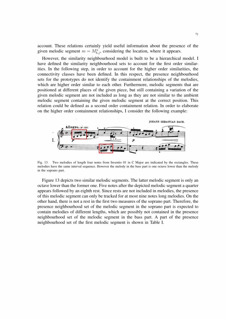
71

account. These relations certainly yield useful information about the presence of thegiven melodic segment m = Mn

k,j , considering the location, where it appears.

However, the similarity neighbourhood model is built to be a hierarchical model. Ihave defined the similarity neighbourhood sets to account for the first order similar-ities. In the following step, in order to account for the higher order similarities, theconnectivity classes have been defined. In this respect, the presence neighbourhoodsets for the prototypes do not identify the containment relationships of the melodies,which are higher order similar to each other. Furthermore, melodic segments that arepositioned at different places of the given piece, but still containing a variation of thegiven melodic segment are not included as long as they are not similar to the ambientmelodic segment containing the given melodic segment at the correct position. Thisrelation could be defined as a second order containment relation. In order to elaborateon the higher order containment relationships, I consider the following example:

Fig. 13. Two melodies of length four notes from Inventio 01 in C Major are indicated by the rectangles. Thesemelodies have the same interval sequence. However the melody in the bass part is one octave lower than the melodyin the soprano part.

Figure 13 depicts two similar melodic segments. The latter melodic segment is only anoctave lower than the former one. Five notes after the depicted melodic segment a quarterappears followed by an eighth rest. Since rests are not included in melodies, the presenceof this melodic segment can only be tracked for at most nine notes long melodies. On theother hand, there is not a rest in the first two measures of the soprano part. Therefore, thepresence neighbourhood set of the melodic segment in the soprano part is expected tocontain melodies of different lengths, which are possibly not contained in the presenceneighbourhood set of the melodic segment in the bass part. A part of the presenceneighbourhood set of the first melodic segment is shown in Table I.

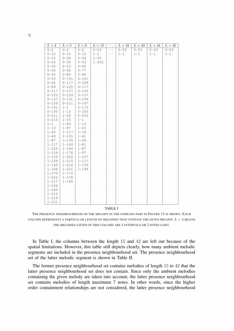
72

L = 4 L = 5 L = 6 L = 12 · · · L = 42 L = 43 L = 44 L = 450-2 0-2 0-2 0-53 · · · 0-53 0-53 0-53 0-530-12 0-12 0-12 1-1 · · · 1-1 1-1 1-1 1-10-20 0-20 0-34 1-250-24 0-30 0-53 1-2020-30 0-53 0-650-34 0-65 0-770-43 0-89 0-890-53 0-101 0-1010-65 0-117 0-1090-89 0-125 0-1170-117 0-137 0-1250-125 0-159 0-1370-137 0-191 0-1590-159 0-211 0-1670-191 1-1 0-1750-195 1-13 0-1830-211 1-25 0-2030-215 1-33 1-11-1 1-49 1-131-13 1-87 1-251-25 1-117 1-331-49 1-125 1-411-87 1-135 1-491-117 1-149 1-611-125 1-166 1-871-129 1-178 1-971-135 1-202 1-1071-139 1-210 1-1171-149 1-218 1-1391-166 1-231 1-1491-170 1-1701-202 1-1781-217 1-1861-1941-2021-2101-2181-231

TABLE I

THE PRESENCE NEIGHBOURHOOD OF THE MELODY IN THE SOPRANO PART IN FIGURE 13 IS SHOWN. EACH

COLUMN REPRESENTS A PARTICULAR LENGTH OF MELODIES THAT CONTAIN THE GIVEN MELODY. L = 4 MEANS

THE MELODIES LISTED IN THIS COLUMN ARE 4 INTERVALS OR 5 NOTES LONG.

In Table I, the columns between the length 15 and 42 are left out because of thespatial limitations. However, this table still depicts clearly, how many ambient melodicsegments are included in the presence neighbourhood set. The presence neighbourhoodset of the latter melodic segment is shown in Table II.

The former presence neighbourhood set contains melodies of length 15 to 42 that thelatter presence neighbourhood set does not contain. Since only the ambient melodiescontaining the given melody are taken into account, the latter presence neighbourhoodset contains melodies of length maximum 7 notes. In other words, since the higherorder containment relationships are not considered, the latter presence neighbourhood

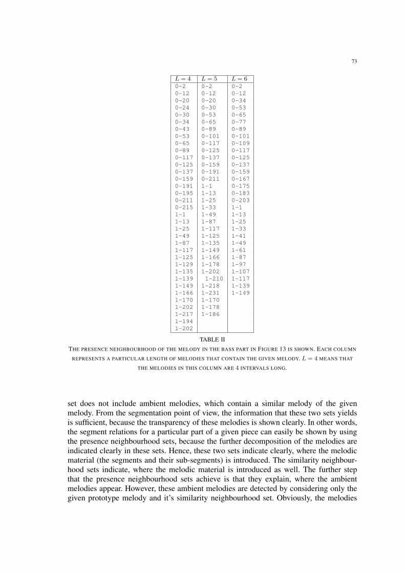
73

L = 4 L = 5 L = 60-2 0-2 0-20-12 0-12 0-120-20 0-20 0-340-24 0-30 0-530-30 0-53 0-650-34 0-65 0-770-43 0-89 0-890-53 0-101 0-1010-65 0-117 0-1090-89 0-125 0-1170-117 0-137 0-1250-125 0-159 0-1370-137 0-191 0-1590-159 0-211 0-1670-191 1-1 0-1750-195 1-13 0-1830-211 1-25 0-2030-215 1-33 1-11-1 1-49 1-131-13 1-87 1-251-25 1-117 1-331-49 1-125 1-411-87 1-135 1-491-117 1-149 1-611-125 1-166 1-871-129 1-178 1-971-135 1-202 1-1071-139 1-210 1-1171-149 1-218 1-1391-166 1-231 1-1491-170 1-1701-202 1-1781-217 1-1861-1941-202

TABLE II

THE PRESENCE NEIGHBOURHOOD OF THE MELODY IN THE BASS PART IN FIGURE 13 IS SHOWN. EACH COLUMN

REPRESENTS A PARTICULAR LENGTH OF MELODIES THAT CONTAIN THE GIVEN MELODY. L = 4 MEANS THAT

THE MELODIES IN THIS COLUMN ARE 4 INTERVALS LONG.

set does not include ambient melodies, which contain a similar melody of the givenmelody. From the segmentation point of view, the information that these two sets yieldsis sufficient, because the transparency of these melodies is shown clearly. In other words,the segment relations for a particular part of a given piece can easily be shown by usingthe presence neighbourhood sets, because the further decomposition of the melodies areindicated clearly in these sets. Hence, these two sets indicate clearly, where the melodicmaterial (the segments and their sub-segments) is introduced. The similarity neighbour-hood sets indicate, where the melodic material is introduced as well. The further stepthat the presence neighbourhood sets achieve is that they explain, where the ambientmelodies appear. However, these ambient melodies are detected by considering only thegiven prototype melody and it’s similarity neighbourhood set. Obviously, the melodies

74

within this similarity neighbourhood set have their own similarity neighbourhood sets.Therefore these melodies have their own ambient spaces. Because of the similarityrelation between these melodies and the given melody, and by pursuing the inheritanceproperty, these ambient spaces can be merged. The merged presence neighbourhood setwould contain ambient melodies of the second order containment relations. Pursuing thisidea in a single-linkage clustering manner (See Section II.5.4), higher order containmentrelationships can be explained by the presence neighbourhood sets.

From a music-theoretical viewpoint, it is also important to see, how the melodicmaterial is used throughout the piece. Since variations of a given melody stem fromthe same material, the ambient melodies containing these melodies happen to use thesame melodic material. Consequently, presence neighbourhood sets considering alsothe higher order containment relationships are able to explain completely, how themelodic material is used. The similarity neighbourhood model defines the higher ordersimilarity relations in terms of connectivity classes. In order to account for the higherorder containment relations, the presence neighbourhood sets for the connectivity classes(See Section II.5.4) should be defined as well.

2) Presence Neighbourhood for the Connectivity Classes: The presence neighbour-hood sets defined for the prototypes consider in the generation of the presence neigh-bourhood sets. In this section, I will introduce the presence neighbourhood sets takingthe higher order similarities between sub- and super-segments into account as well.

Definition 2.27: The presence n’-neighbourhood for the connectivity class Enc (M)

(consisting of melodies of length n) is defined to be the union of those connectivityclasses En′

d (M) (each consisting of melodies of length n′) containing a melodic segmentm′, such that a melodic segment m in the connectivity class En

c (M) is a sub-segmentof m′. The presence neighbourhood for the connectivity class En

c (M) is the unionof all presence n’-neighbourhood sets where n′ ∈]length(m), length(M)]:

PEqn′

(Enc (M)) =

⋃m′∈En′

d (M)m∈En

c (M)

En′

d (M)|m = m′ni ,

PEq(Enc (M)) =

⋃PEq

n′(En

c (M)).

In comparison to the presence neighbourhood sets for the prototypes, the presenceneighbourhood sets for the connectivity classes consider every single melody within theconnectivity class and the ambient melodies containing them. Hence, the connectivityclasses of the ambient melodies containing a melody from the given connectivity classare united. Therefore the higher order similarities among the contained melodies aswell as among the ambient melodies are taken into account, which in turn accounts forhigher order containment relationships as well.

Since a connectivity class already contains first- and higher-order similarities betweenequal length melodies, I do not define weak and strong presence neighbourhood sets.Furthermore, connectivity classes are defined to unite similar melodies. Defining weak

75

and / or strong neighbourhoods would break this principle. In this respect, through theconnectivity classes, this principle of unification is extended to the sub- and super-segment relationships as well.

The presence n’-neighbourhood sets for a particular connectivity class eventuallyconsist of several connectivity classes, due to the fact that two melodies containing thesame melody can possibly belong to separate connectivity classes. In this case, both ofthese connectivity classes are included into the presence n’-neighbourhood set of thegiven connectivity class. However, the following result helps to make inferences aboutthe construction of the presence neighbourhood sets of the connectivity classes.

Corollary 2.2: Suppose that there are two melodic segments m = Mnk1,i+j and m =

Mnk2,i′+j ∈ En

c (M) such that they are contained by the sub-segments Mn′

k1,i and Mn′

k2,i′ oflength n′ at analogous positions i+ j and i′ + j respectively. These two super-segmentsMn′

k1,i and Mn′

k2,i′ belong to the same connectivity class En′

d (M), if the second part ofthe inheritance property holds.

The similarity relation between two melodic segments does not necessarily imply asimilarity between their super-segments. The inheritance property is necessary in orderthis statement to be true. Hence, Corollary 2.2 mathematically formulates the necessityof the inheritance property to imply a similarity relation between the super-segments oftwo similar melodic segments.

3. The Content Neighbourhood

Naively speaking, the content of a given melody is the set of all segments of themelody. These segments naturally appear within the given melody, where-ever the givenmelody literally appears. However, some of the segments of the given melody alsoappear independently, and some similar occurrences of a melody do not necessarilycontain similar sub-segments. The content neighbourhood aims to identify particularlythe segments of a given melody up to similarity.

Buteau [14] and Mazzola [49] also defined a content function. Similar to the case inthe presence function, the content function simply counts the number of sub-segmentsof a given melody. The quantity that this function yields gives clues about how oftenthe melodic material(sub-segments of the given melody) of a given melody is usedthroughout the piece. In other words, this value can be considered to be a prominencevalue of the given melody. However, the locations of, where these sub-segments appearis not delivered by this function. Music-theoretically speaking, form a form analysispoint of view, the places, where the sub-segments appear are important, in order to beable to determine the form of the piece. For this reason, I re-defined the content functionas a neighbourhood set called the content neighbourhood not only counting the numberof appearances of the sub-segments (The cardinality of the set gives this information.),but also indicates, where these sub-segments appear within the given piece.

1) Content Neighbourhood for the Prototypes: As in the presence neighbourhoodsets, I consider the content neighbourhood sets on the prototypes level at first. The

76

content neighbourhood sets on the connectivity classes level will be defined afterwards.

Definition 2.28: The set of all segments of length n′ similar to a prominent sub-segment m′ = Mn′

k,j+i−1 of a given melodic segment m = Mnk,j , such that m′ = mn′

i

and 0 < i ≤ n − n′ + 1, is called the weak content n’-neighbourhood of the givenmelody. The weak content neighbourhood of a given melody m is the union of all ofthe content n′-neighbourhood sets for:

n ∈ [minimum melody length, length(m)[.


Conn′(m,M) =⋃

m′=mn′i

UR(m′, M), (35)

Con(m, M) =⋃{Conn(m,M)}. (36)

The content neighbourhood includes the complete set of sub-segments of the givenmelody and their similar melodies within the given piece. The index i of the sub-segments is controlled to be in the interval (0, n−n′ + 1], so that the sub-segments arecontained by the given melody m completely.

The complete content of a given melodic segment is generated by unifying the weakcontent n′-neighbourhood sets. This unification collects the sub-segments of the givenmelodic segment and their similar melodic segments together.

A weak content neighbourhood set contains only the sub-segments of a given melodicsegment and similar melodies to those sub-segments. However, it is not consideredwhether the melodic segments containing those sub-segments are similar to the givenmelodic segment m or not. In other words, the inheritance property is not forced forthe weak content neighbourhood set. In order to account for the inheritance property,the strong content neighbourhood set of a given melodic segment is defined as follows:

Definition 2.29: The strong content n’-neighbourhood of a given melodic segmentm = Mn

k,j contains only those similar sub-segments m′ from the weak content n’-neighbour-hood, such that m′ = mn′

i and 0 < i ≤ n − n′ + 1, so that the melodiesanalogously containing these segments are also similar to the given melodic segment.The strong content neighbourhood of the given melodic segment m is the union ofall of the strong content n′-neighbourhood sets for:

n ∈ [minimum melody length, length(m)[.


77

Conn′(m, M) =

⋃m′=mn′

i

{m′′n′

i ∈ Un′

R (m′, M)|m′′ ∈ UnR(m,M)}, (37)

Con(m, M) =⋃{Conn

R(m, M)}. (38)

The strong content neighbourhood contains the complete set of sub-segments of thegiven melodic segment m and their similar melodic segments within the given piece.This neighbourhood set obeys the inheritance property, because only the sub-segmentsare taken into the strong neighbourhood set, whose super-segments are similar to m.

The content neighbourhood sets for the prototypes consider the similarity neigh-bourhood sets only. This way, a given melodic segment can be decomposed into sub-segments properly, depending on the similarities defined by the similarity neighbourhoodset and on the sub-segments. The sub-segment relationships between the first-ordersimilar melodies can be identified that way. In order to account for the sub-segmentrelationships between the higher order similar melodies, the content neighbourhood setsfor the connectivity classes are defined.

2) Content Neighbourhood for the Connectivity Classes: The content neighbourhoodsets for the connectivity classes consider the higher order similarities as well as the firstorder similarities in explaining how the melodic content of a complete connectivityclass is used throughout the piece. In other words, not only the higher order similaritiesbetween the sub-segments are taken into account, but also the melodic material (content)is also constructed by using the higher order similarities.

Definition 2.30: The content n’-neighbourhood for the connectivity class Enc (M) of

melodies of length n is defined to be the connectivity classes En′

d (M) of melodies oflength n′ ( with n′ < n), each of which containing at least one melodic segment m′,such that m′ is a sub-segment of a melodic segment m in the connectivity class En

c (M).The content neighbourhood for the connectivity class En

c (M) is the union of the contentn’-neighbourhood sets for n ∈ [minimum melody length, length(m∗)[:

CEqn(En

c (M)) =⋃

m′∈En′d (M)

m∈Enc (M)

En′

d (M)|m′ = mn′

i ,

CEq(Enc (M)) =

⋃CEq

n(Enc (M)).

The content neighbourhood sets for the connectivity classes are not defined as weak-and strong neighbourhood sets. Similar to the presence neighbourhood sets for theconnectivity classes, the higher order similar melodies are collected in a connectivityclass. Separating the connectivity classes as weak- and strong sets would harm thisconnectivity. Therefore, I defined the content neighbourhood sets as well as the presenceneighbourhood sets for a connectivity class without the distinction of weak and strong.

The content n′-neighbourhood sets of a given connectivity class can contain more thanone connectivity classes depending on the first- and higher-order similarities between

78

the sub- and super-segments. The following corollary explains the role of the inheritanceproperty in the construction of these sets.

Corollary 2.3: Suppose that there are two melodic segments Mnk1,i and Mn

k2,i′ oflength n which belong to the same connectivity class En

c (M), such that they containthe sub-segments Mn′

k1,i+j and Mn′

k2,i′+j of length n′ at analogous positions i + j andi′ + j respectively. These two sub-segments Mn′

k1,i+j and Mn′

k2,i′+j belong to the sameconnectivity class En′

d (M), if the first part of the inheritance property holds.

During the construction of the connectivity classes, all of the first- and higher-ordersimilar melodies are collected in the same connectivity class. However, the inheritanceproperty does not have an influence on constructing the connectivity classes. It does nothave an influence on the relationships between the connectivity classes either. Hence, itis not possible to enforce the inheritance property in this case. However, the condition istrue that if the second part of the inheritance property holds, for two similar melodies,their super-melodies should be contained in the same connectivity class.

4. Theoretical Findings about the Sub-Segment Relationships

The sub-segment relations defined in Sections II.7.2 and II.7.3 imply some impor-tant results. These results will be used in Chapter VII for investigating the similarityneighbourhood model from a topological viewpoint.

The first result indicates the relation between the presence and the content neighbour-hood sets for the corresponding melodic segments, which contain each other. Logically,the containing melody appears within the presence neighbourhood set of the containedmelody. In the same way, the contained melody is included in the content neighbourhoodset of the containing melody. This relationship is defined formally as follows:

Lemma 2.1: Given two melodic segments m ∈ P n and m′ ∈ P n′ , such that m =m′n

i , then the following is true:

m ∈ Conn(m′, M) and m ∈ Conn(m′, M), (39)

m′ ∈ P resn′(m, M) and m′ ∈ Presn′(m, M). (40)

This result implies also that the presence and content neighbourhood sets for twomelodic segments having a sub-segment relation with each other are two differentviewpoints for this relationship. For the longer melodic segment, the shorter melodicsegment is the content of the longer melodic segment. For the shorter melodic segment,the longer melodic segment is the presence of the shorter melodic segment within thelonger melodic segment. But from both viewpoints, it is the same sub-segment relationinterpreted differently.

The second result implies the inheritance property from a different viewpoint. Itstates in which conditions the melodic segments belong to the corresponding presence

79

or content neighbourhood sets. This statement also implies in which conditions theinheritance property holds.

Lemma 2.2: Given two melodic segments m ∈ P n and m′ ∈ P n′ , such that m =m′n

i , if for any two melodies m and m′, the following holds

m = m′ni (41)

m ∈ UR(m,M) and m′ ∈ URn′ (m′, M), (42)

then the following is true

m ∈ Conn(m′, M), (43)m′ ∈ Presn′

(m,M). (44)

As a result of the statement above the following can be deduced:

Corollary 2.4: The Lemma 2.2 implies that the inheritance property holds forConn(m′, M) and Presn′

(m,M) sets.

The Corollary 2.4 implies that the concerned presence and content neighbourhood setsare both strong. Furthermore, if the sub-segment Condition 41 within the Lemma 2.2 isnot true, for the melodic segments m and m′, the presence and content neighbourhoodsets are weak.

If the cardinalities of the presence- and content neighbourhood sets are considered,the following can be observed:

Lemma 2.3: For a given melodic segment m ∈ P n of length n, the cardinality ofthe weak presence n’-neighbourhood is equal to the sum of the cardinalities of thesimilarity neighbourhood sets of the ambient melodic segments m′ ∈ P n′ containingthe given melodic segment:

card(P resn′(m,M)) =n′−n+1∑

i=1

card(U(m′, M)), where m = m′ni . (45)

The weak presence n’-neighbourhood set of a given melodic segment is by definitionthe similarity neighbourhood set of an ambient melodic segment. Therefore, the cardi-nality of the weak presence n′-neighbourhood set of the given melodic segment m issimply the sum of the cardinalities of the similarity neighbourhood sets of the melodicsegments containing the given melodic segment. However, the same cannot be claimedfor the strong presence n’-neighbourhood sets. Since the inheritance property must holdfor the strong presence n′-neighbourhood sets, some of the melodies are possibly leftout from the weak presence n′-neighbourhood sets. Therefore they are smaller than thesum of the cardinalities of the similarity neighbourhood sets of the containing melodicsegments:

Lemma 2.4: For a given melodic segment m ∈ P n of length n, the cardinality of thestrong presence n’-neighbourhood is less than or equal to the sum of the cardinalities of

80

the similarity neighbourhood sets of the ambient melodic segments m′ ∈ P n′ containingthe given melodic segment:

card(P resn′(m, M)) ≤n′−n+1∑

i=1

card(U(m′, M)), where m = m′ni . (46)

As the Lemma 2.1 also implies, the statements of Lemmas 2.3 and 2.4 are also truefor the content n′-neighbourhood sets.

II.8. THE PROMINENCE MATRIX

Using the prominence profile in co-operation with the neighbourhood sets defined inthe section II.4 the prominence matrix of the piece is obtained. The prominence matrixis indicated by S.

Before defining the prominence matrix, the combination of the prominence profileand neighbourhood sets should be clarified. Hence, the elements of the prominencematrix are defined as follows:

pnn =

∑m∈M card(Un

R(m,M)) where length(m) = n,

pn+1n =

∑m∈M card(U

n+1

R (m, M)) where length(m) = n,pn−1

n=

∑m∈M card(Un−1

R (m, M)) where length(m) = n.(47)

The diagonal elements of the prominence matrix, namely the function pnn contains the

sum of the cardinalities of the similarity neighbourhood of the prototypical melodies oflength n. The other two functions, namely pn+1

n and pn−1n

are the number of elements ofthe presence and content neighbourhoods of the melodies of length n correspondingly.Under the light of these definitions, the prominence matrix is defined as follows:

S =

p1

1 p21 . . . . . . . . .

......

......

.... . . pn−1

npn

n pn+1n . . .

......

...... . . .

(48)

The diagonal of the matrix is constituted by the total number of melodies containedin the similarity neighbourhoods. The upper triangular matrix contains the total numberof melodies from the presence neighbourhood of melodies on the diagonal and thelower triangular matrix the total number of melodies from the content neighbourhoodof the same melodies. In this respect, the prominence matrix can be considered asthe interpretation of the presence and content functions (See Sections II.7.2 and II.7.3)defined by Buteau [14] and Mazzola [49], in order to explain the sub- and super-segmentrelationships between the melodies within a given piece.

81

II.9. REDUCTION METHODS FOR THE REDUNDANT MELODIES

Ruwet [67] presents a method for paradigmatic partitioning starting with the identi-fication of the longest repeated segments within a given piece. In the following steps,Ruwet identifies shorter segments as well as sub-segments of the previously identifiedlonger segments, which partition the given piece any further. That is to say, the shortersegments or the sub-segments of the longer segments help to decrease the amount ofthe unpartitioned parts of the given piece by defining new partitions in those areas. Thefollowing strategy employs these ideas of Ruwet in a more general situation, where thesegments are not strictly partitioning.

From the similarity point of view, within every repetition of a melody, its sub-melodies are repeated as well. However, these repetitions neither contribute to thepartitioning of the given piece nor explain the usage of the melodic material introduced.Pursuing Ruwet’s ideas, longest repeated segments are identified, which contribute tothe partitioning of the given piece. The repetitions of their sub-segments within thesesegments are detected, and identified as redundant for the melodic development of thepiece [6]. In the similarity neighbourhood model, a melodic segment being in such aredundant situation is defined as follows:

Definition 2.31: A melodic segment is called redundant, if there is a longer melodicsegment containing the given melodic segment, up to similarity, wherever the givenmelodic segment appears.

Due to the exhaustive nature, the similarity neighbourhood model identifies the re-dundant melodic segments as well. However, these melodic segments can be removedfrom the set of the results. The identification and elimination of redundant melodies isbased on the inheritance principle (See Section II.7.1).

1. Weak Reduction

The weak reduction is applied to the entire collection of neighbourhoods, in order toyield an analogous family of neighbourhoods. It is defined as follows:

Definition 2.32: Given two melodic segments m = Mnk,i and m = Mn′

k,j of length n

and n′ respectively, where m′ = mn′j (with j + n′− 1 ≤ n). The melody m′ is removed

from the results, ifcard(Un′

R (m′, M)) ≤ card(UnR(m, M))

.

According to the Definition 2.32, a melodic segment is removed, if the number of it’soccurrences is less than or equal to the number of occurrences of the melodic segmentcontaining it. Intuitively, the number of appearances of redundant melody is equal toor less than the number of appearances of one of its ambient melodies, because theseappearances are expected to be within this particular ambient melody. However this does

82

not have to be true for all the cases, because the first part of the inheritance propertyis not checked for the weak reduction. This can be intuitively proven as follows:

Proof: Assume that there exists a melodic segment m′′, such that

m′′ ∈ Un′R (m′, M) and m′′ = m′′′n′

i .

If ||m′′′|| = ||m|| and m′′′ /∈ UnR(m, M), then the inheritance property does not hold.

The Proof of Definition 2.32 shows that the reduced melodic segment does nothave to appear only within a particular ambient melodic segment, but can appearindependently as well. Therefore, the inheritance property does not hold for these twomelodic segments considering the sub- and super-segment relationships. For this reason,this reduction method is called the weak reduction.

From music-theoretical point of view, melodies appearing not only within their super-segments but also independently within the given musical piece are important for thisparticular musical piece. These kinds of melodies should not be removed. On thecontrary, they should be kept in the results, and investigated further.

2. Strong Reduction

Before reducing a melody, considering only the number of appearances, the firstpart of the inheritance property should be checked as well. For this reason, anotherreduction method is defined, which investigates every single appearance of the givenmelody, in order to figure out whether the melody appears independently as well.The melodies appearing independently (not only within their super-segments) are notreduced. Therefore the resulting reduction method, which is called the strong reduction,satisfies the inheritance property. The strong reduction is defined as follows:

Definition 2.33: Given two melodic segments m = Mnk,i and m = Mn′

k,j of length n

and n′ respectively, where m′ = mn′j (with j + n′− 1 ≤ n). The melody m′ is removed

from results, ifcard(Un′

R (m′, M)) ≤ card(UnR(m, M))

, and if for all melodic segments m′ ∈ Un′R (m′, M), there exists a melodic segment

m ∈ UnR(m, M) such that m′′ = mn′

j

.

The second reduction method satisfies the inheritance property. The employed con-dition guarantees that just the melodic segments are removed from the analysis, whichappear only within a particular ambient melody at analogous positions. Conforming tothe terminology I used so far, because this reduction method satisfies the inheritanceproperty, it is called the strong reduction.

83

These two reduction methods incorporate the sub-segment relationships of melodicsegments to identify the redundant ones. The following theorems combine these relation-ships with the presence / content neighbourhoods of the concerned melodic segments:

Theorem 1: If a given melodic segment m′ ∈ P n′ is reduced by the weak reductionmethod, for at least one particular length n > n′, the following is true:

card(Un′

R (m′, M)) <= card(P resn(m′, M)).

By definition, the similarity neighbourhood sets of the ambient melodic segments areunited in the weak presence neighbourhood set of the given melodic segment. In theextreme case, for a particular length n, the weak presence neighbourhood set of the givenmelody contains only one similarity neighbourhood set. In other words, there is onlyone ambient melody, which contains the given melody. According to the Lemma 2.3,the comparison of the cardinalities of the similarity neighbourhood sets implies thecomparison of the cardinality of the similarity neighbourhood set of the melodic seg-ment to be reduced with the cardinality of the weak presence n’-neighbourhood set.Consequently, even in the extreme case, the cardinality of the similarity neighbourhoodset of the given melody is less than the cardinality of the similarity neighbourhood setof the only ambient melody (, which is in turn the cardinality of the weak presenceneighbourhood set of the given melodic segment.).

A similar statement can be drawn for the strong reduction case.

Theorem 2: If a given melodic segment m′ ∈ P n′ is reduced by the strong reductionmethod, for at least one particular length n > n′, the following is true:

card(Un′

R (m′, M)) <= card(Presn(m′, M)).

The strong presence neighbourhood of a given melodic segment contains only themelodic segments, whose corresponding sub-segments are similar to the given melodicsegment. Considering the additional condition of the strong reduction definition, amelodic segment is then reduced, if it only appears within another melodic segmentcontaining it. In other words, if a given melodic segment and its similar segmentsappear only within a particular super-segment and its similar melodies, the given melodicsegment is reduced. Hence, a melodic segment is reduced strongly, if and only if allappearances of it are contained by the melodies within a particular strong presencen-neighbourhood set of the same melodic segment for a particular length.

Consequently, if a melodic segment is eliminated from the results, the number ofappearances of a melodic segment is less than the number of appearances of the melodicsegments, within which it is present. Even-though the obtained set of results are stillparadigmatic in nature, the reduction process still makes one step in the direction ofsyntagmatic analysis of music. Therefore in the following pages, the reduced resultswill be called syntagms.

84

II.10. IMPLEMENTATION DETAILS

Connectivity classes and representatives are constructed separately for melodies ofdifferent lengths. Depending on the experiments described in Section II.3.3.1, the short-est pitch sequences are determined to be four intervals long (five consecutive pitches).The longest sequences are as long as the longest passage without a rest within the givenpiece. For every length n, I consider all consecutive pitch sequences of length n usinga sliding window, starting from the sequence defined by the first n notes of the firstvoice until the last notes of the last voice are reached. For each of these melodies, allequal length melodies within each voice are searched, and a similarity neighbourhoodis constructed. Similarity neighbourhoods are then processed to obtain the connectivityclasses, the representative melodies, and the prominence profile. The complete algorithmis given as follows:

In the following algorithm, the variable names begin with capital letters. The constantsare written in capital letters.

1) Initialise parametersa) Initialise MINIMUM_LENGTHb) Initialise CORRELATION_CONSTANTc) Initialise SIGNIFICANCE_CONSTANT

2) For Each Part of the Given Piecea) For Each Length of the Melodies in the Current Part, Starting with MINIMUM_LENGTH

i) Calculate CorrelationThresholdii) Calculate SignifinanceThreshold

iii) For Each MelodyA) Calculate Similarity Neighbourhood SetB) Calculate SignificanceC) if Significance > SignificanceThreshold

Mark Melody as Prototypeiv) Calculate Connectivity Classes

3) Calculate Presence Neighbourhood Sets4) Calculate Content Neighbourhood Sets5) Calculate the Prominence Profiles of the Piece

In the given algorithm, parts (voices) are handled separately one after the other.Hence, starting with the lowest part, every single melody in this part is analysed, beforemoving to the next part. However for each melody, all of the parts of the given pieceare traversed.

The algorithm does not show the detailed steps of the reduction procedure. However,after the presence and content neighbourhoods have been calculated for each melodywithin the piece, the reduction process is applied. For the weak and strong reductionthe prominence profiles are calculated again.

In the implementation, I used the Humdrum Software System (See Appendix A) torepresent musical pieces and to extract information from them. In order to visualise and

85

play the results Open Music Software was used (See Appendix B).

The similarity neighbourhood sets, ignoring the generation of the connectivity classes,are generated inO(n3) time. For each length value, there are n melodies to be analysed.Each melody is compared to each other melody. Therefore this analysis step takes O(n2)time. Since there are n different length values, the complete similarity neighbourhoodanalysis is performed in O(n3) time.

86

87

III. AN EVOLUTIONARYAPPROXIMATION TO THE SIMILARITY

NEIGHBOURHOOD MODEL

III.1. INTRODUCTION

The similarity neighbourhood model is an exhaustive analysis model in nature. Duringthe analysis, it traverses a given musical piece for each melody repeatedly to constructthe similarity neighbourhood sets. This analysis step yields the melodic structure of agiven piece from the similarity point of view. As explained in the previous sections,the model builds the connectivity classes, sub-segment relationships and the reductionhierarchically on top of the similarity neighbourhood sets. Since only consecutive notesexcluding the rests are considered to be a melody, the model produces these results ina reasonable time.

In general, optimisation techniques are applied to estimate the outputs of an unknownfunction, which cannot be calculated analytically or to determine the unknown classboundaries of a classification task. Furthermore, they can be incorporated to approximatethe results of an exhaustive model without loosing the relevant information. Such anapproximation provides a certain degree of acceleration in the calculations as well.Even-though the original similarity neighbourhood model works efficiently, making useof such an acceleration is of significant help, especially for very long musical piecessuch as those consisting of four or five voices.

Such a search problem can make use of parallelism, in which many different possiblesolutions are explored simultaneously in an efficient manner. Besides computationalparallelism, which is needed to evaluate these possible solutions simultaneously, anintelligent strategy is also required to select the next set of possible solutions to evaluate.Instead of evaluating every possible candidate solution, an efficient selection strategyincorporated to select better candidate solutions accelerates an exhaustive model a sig-nificant amount. Genetic algorithms [55] [54] offer a probabilistic strategy to select andevaluate possible solutions of a given problem by mimicking the biological evolution.

There are certainly other optimisation methods, which could be used for acceleratingthe similarity neighbourhood model. However standard gradient based optimisationmethods make a search in the solution domain, in order to find a single optimal solution.They mostly assume that there is a correlation between the solutions that are closeto each other in the search space. Genetic algorithms make use of the best qualityparent solutions in the search space, and combine them to produce a new generation ofcandidate solutions. In the end, genetic algorithms generate a population of high qualitysolutions, not a single optimal solution. Since the similarity neighbourhood model ex-

88

tracts the melodic structure of a given piece, which consists of significant melodies, i.e.,a population of significant melodies, genetic algorithms offer an appropriate method toaccelerate the similarity neighbourhood model. Therefore, the similarity neighbourhoodmodel has been accelerated by genetic algorithms [4].

A stochastically generated group of melodies are evaluated to find the significant ones.By randomly selecting melodies from the current group, and applying some geneticoperators on them, new group of melodies are generated. By improving the qualityof these groups iteratively, the most significant melodies are extracted to construct theprominence profile of a piece as defined in the similarity neighbourhood model.

Obviously, the genetic algorithms only approximate the original similarity neighbour-hood model. However, the experiments have shown that this approximation yields goodresults in a significantly less time compared to the exhaustive model.

III.2. GENETIC ALGORITHMS

The problem addressed by genetic algorithms is to search a space of possible solutionsto identify the best collection of solution. In each iteration, genetic algorithms evaluatea set of possible solutions. Depending on the evaluation results, the algorithm generatessuccessor solutions by probabilistically selecting better solutions among the whole set ofsolutions, and applying some so-called genetic operators on them. After each evaluationstep, a collection of possible solutions called the current population is replaced by anew population.

A population contains possible solutions to a given problem, The possible solutions,each called a chromosome, generally take the form of constant length bit strings.Genetic algorithms proceed by evaluating each chromosome in the population, andreplacing a population afterwards with another, until the termination criteria is fulfilled.A population of chromosomes is defined as follows:

Pi = {c1, c2, · · · cs} (49)

In this formulation, the population Pi contains s number of chromosomes eachindicated by cj , where j is the index of a chromosome c within the current populationi. The population index i indicates the current iteration of genetic algorithms. In thefollowing iteration, population Pi is going to be replaced by the new population Pi+1.

The chromosomes are evaluated by a so-called fitness function. This function assignsa numeric value to each chromosome that indicates how well this chromosome solvesa given problem.

After each evaluation step of the population, a better population is expected to becreated, which contains chromosomes that are more fit than the chromosomes in theprevious population. For the generation of the new population, three genetic operatorsare defined.

89

The selection operator probabilistically selects chromosomes for reproduction. Themore fit the chromosome, the more likely it is to be selected. The probability of selectinga chromosome ci is given by

Pr(ci) =Fitness(ci)∑s

j=1 Fitness(cj)(50)

The crossover operator selects two chromosomes and exchanges parts of the chro-mosomes to create two new offspring. The parts to be exchanged are selected proba-bilistically as well.

The last genetic operator is called mutation. This operator probabilistically selects achromosome, and randomly flips some of the bits in the selected chromosome.

Consequently, a new population is generated by probabilistically selecting the morefit chromosomes from the previous population. Some of the selected chromosomes aredirectly added to the new population. Crossover or mutation operators are applied ontothe others to generate new offspring. These new offspring are inserted into the newpopulation.

Genetic algorithms iteratively search the solution space by evaluating candidate so-lutions contained in the current population, and improving the quality of this collectionafter each iteration for a desired solution.

The similarity neighbourhood model has partly been adapted to genetic algorithmsso that they can be incorporated to evaluate the quality of the selected melodies. Hencethe definition of melodies are adapted in the way that they can be processed by geneticalgorithms. A population consists of melodies of different length as candidate solutions.These melodies are evaluated by generating their similarity neighbourhood sets andcalculating the corresponding significance values. The adaptation of the similarity neigh-bourhood model enables the application of the genetic operators, in order to generatethe next population among the melodies constituting the current population.

1. Representation of a Melody

In order to use melodies as candidate solutions, they must be represented by constantlength vectors, so that the genetic operators can be applied on them. The definition ofmelodies as in the similarity neighbourhood model cannot be used, because in the sim-ilarity neighbourhood model, melodies of different length are represented by sequencesof different length. Hence, the definition of a melody in the similarity neighbourhoodmodel is adapted to genetic algorithms as follows:

Definition 3.1: A melody mj = Mnk,i of length n within the voice k of a given piece

M is a 3-tuple of integer variables as follows:

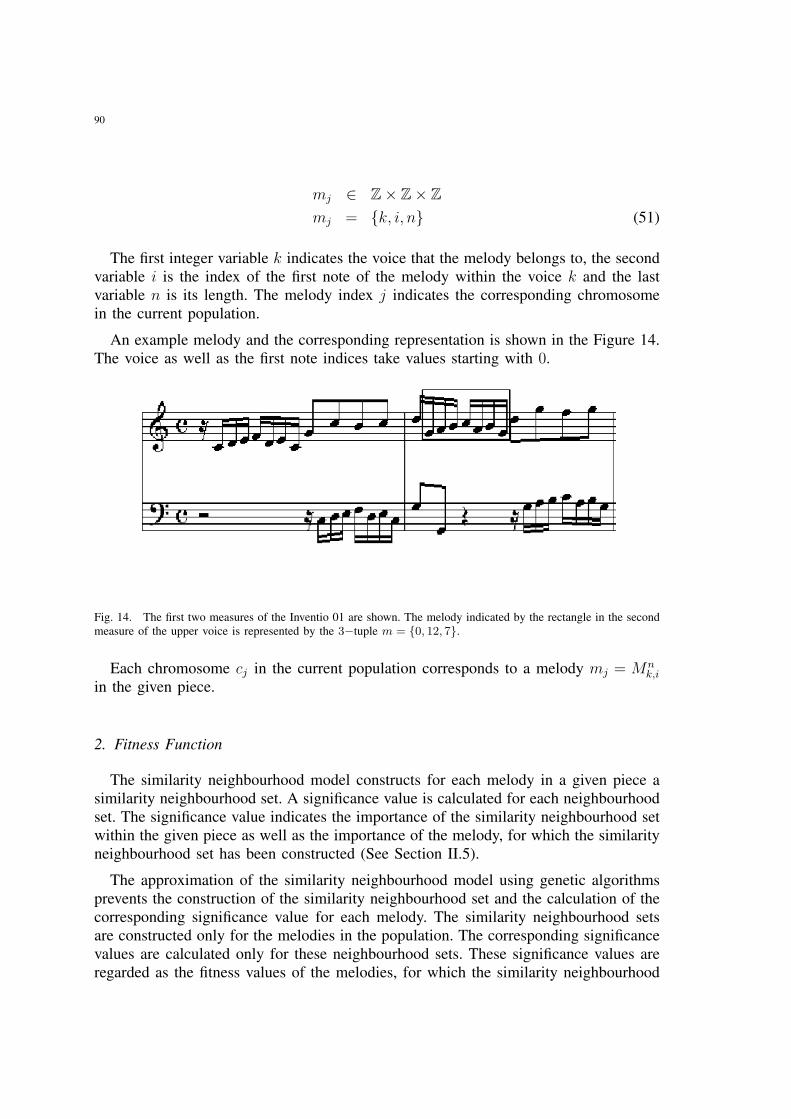
90

mj ∈ Z× Z× Zmj = {k, i, n} (51)

The first integer variable k indicates the voice that the melody belongs to, the secondvariable i is the index of the first note of the melody within the voice k and the lastvariable n is its length. The melody index j indicates the corresponding chromosomein the current population.

An example melody and the corresponding representation is shown in the Figure 14.The voice as well as the first note indices take values starting with 0.

Fig. 14. The first two measures of the Inventio 01 are shown. The melody indicated by the rectangle in the secondmeasure of the upper voice is represented by the 3−tuple m = {0, 12, 7}.

Each chromosome cj in the current population corresponds to a melody mj = Mnk,i

in the given piece.

2. Fitness Function

The similarity neighbourhood model constructs for each melody in a given piece asimilarity neighbourhood set. A significance value is calculated for each neighbourhoodset. The significance value indicates the importance of the similarity neighbourhood setwithin the given piece as well as the importance of the melody, for which the similarityneighbourhood set has been constructed (See Section II.5).

The approximation of the similarity neighbourhood model using genetic algorithmsprevents the construction of the similarity neighbourhood set and the calculation of thecorresponding significance value for each melody. The similarity neighbourhood setsare constructed only for the melodies in the population. The corresponding significancevalues are calculated only for these neighbourhood sets. These significance values areregarded as the fitness values of the melodies, for which the similarity neighbourhood

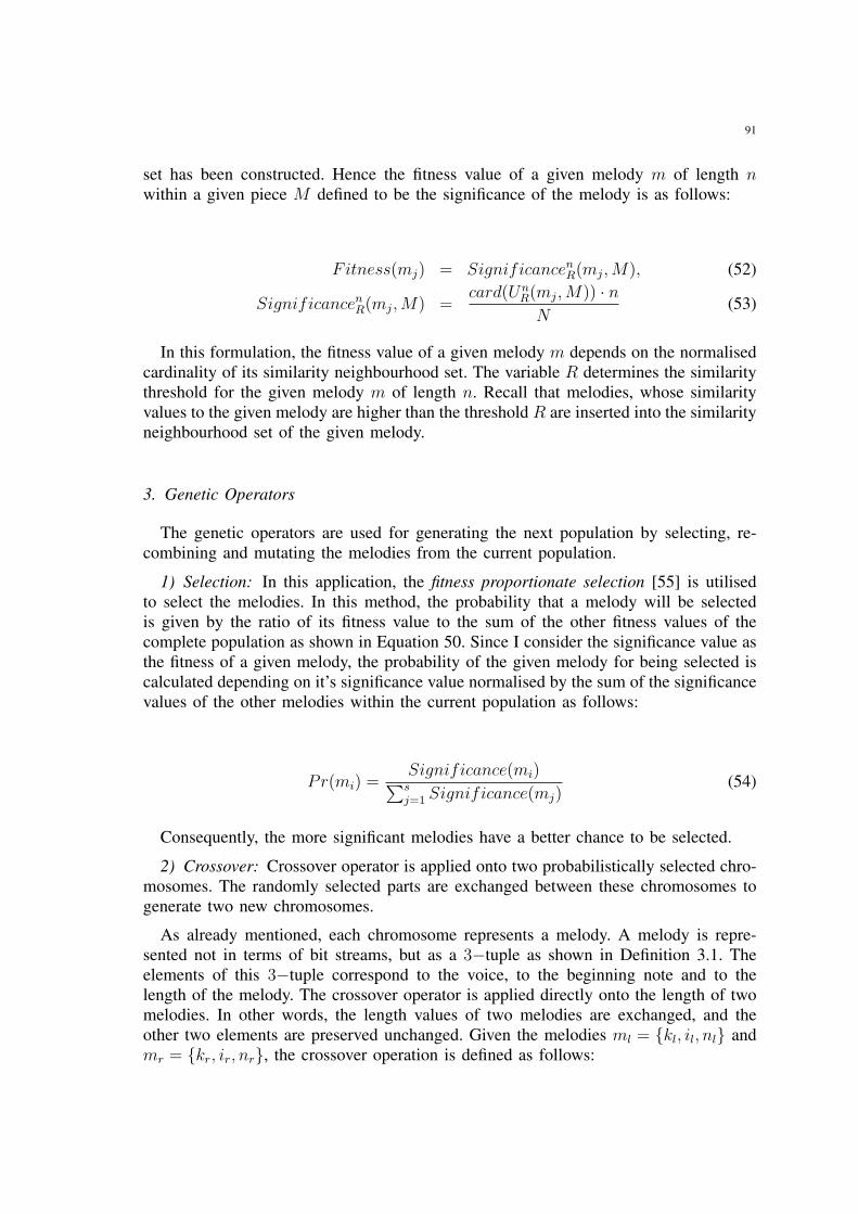
91

set has been constructed. Hence the fitness value of a given melody m of length nwithin a given piece M defined to be the significance of the melody is as follows:

Fitness(mj) = SignificancenR(mj, M), (52)

SignificancenR(mj, M) =

card(UnR(mj, M)) · n

N(53)

In this formulation, the fitness value of a given melody m depends on the normalisedcardinality of its similarity neighbourhood set. The variable R determines the similaritythreshold for the given melody m of length n. Recall that melodies, whose similarityvalues to the given melody are higher than the threshold R are inserted into the similarityneighbourhood set of the given melody.

3. Genetic Operators

The genetic operators are used for generating the next population by selecting, re-combining and mutating the melodies from the current population.

1) Selection: In this application, the fitness proportionate selection [55] is utilisedto select the melodies. In this method, the probability that a melody will be selectedis given by the ratio of its fitness value to the sum of the other fitness values of thecomplete population as shown in Equation 50. Since I consider the significance value asthe fitness of a given melody, the probability of the given melody for being selected iscalculated depending on it’s significance value normalised by the sum of the significancevalues of the other melodies within the current population as follows:

Pr(mi) =Significance(mi)∑s

j=1 Significance(mj)(54)

Consequently, the more significant melodies have a better chance to be selected.

2) Crossover: Crossover operator is applied onto two probabilistically selected chro-mosomes. The randomly selected parts are exchanged between these chromosomes togenerate two new chromosomes.

As already mentioned, each chromosome represents a melody. A melody is repre-sented not in terms of bit streams, but as a 3−tuple as shown in Definition 3.1. Theelements of this 3−tuple correspond to the voice, to the beginning note and to thelength of the melody. The crossover operator is applied directly onto the length of twomelodies. In other words, the length values of two melodies are exchanged, and theother two elements are preserved unchanged. Given the melodies ml = {kl, il, nl} andmr = {kr, ir, nr}, the crossover operation is defined as follows:

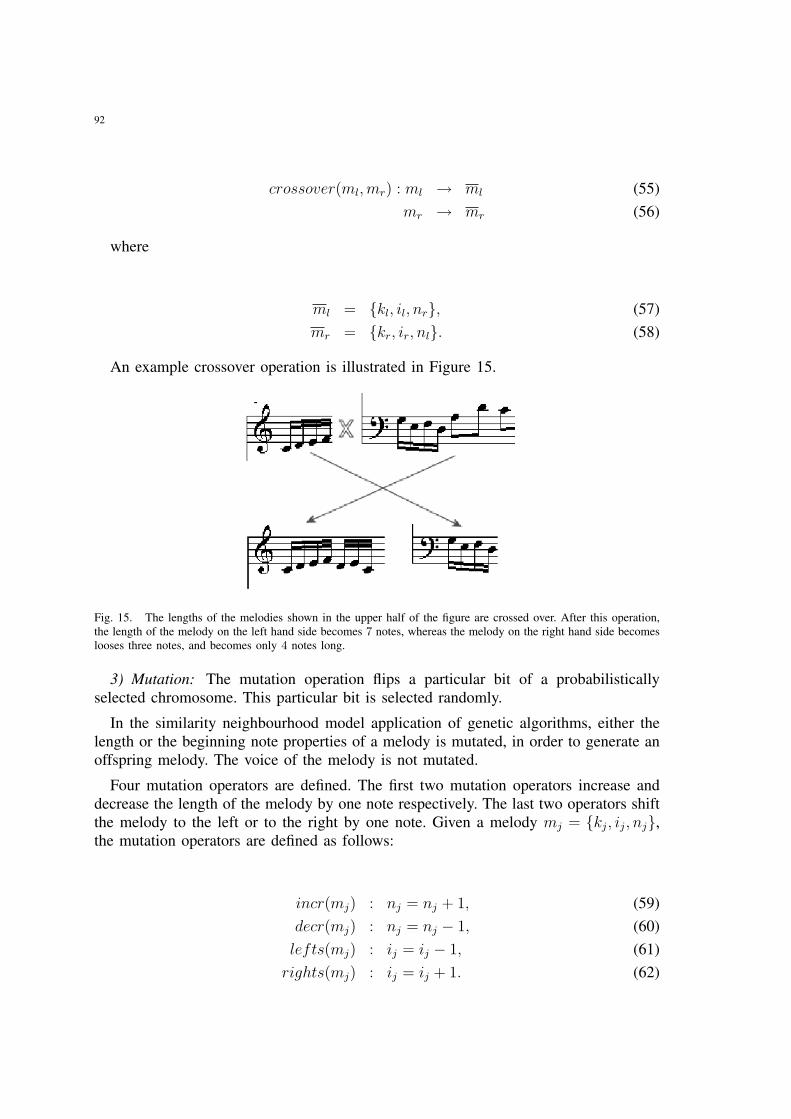
92

crossover(ml, mr) : ml → ml (55)mr → mr (56)

where

ml = {kl, il, nr}, (57)mr = {kr, ir, nl}. (58)

An example crossover operation is illustrated in Figure 15.

Fig. 15. The lengths of the melodies shown in the upper half of the figure are crossed over. After this operation,the length of the melody on the left hand side becomes 7 notes, whereas the melody on the right hand side becomeslooses three notes, and becomes only 4 notes long.

3) Mutation: The mutation operation flips a particular bit of a probabilisticallyselected chromosome. This particular bit is selected randomly.

In the similarity neighbourhood model application of genetic algorithms, either thelength or the beginning note properties of a melody is mutated, in order to generate anoffspring melody. The voice of the melody is not mutated.

Four mutation operators are defined. The first two mutation operators increase anddecrease the length of the melody by one note respectively. The last two operators shiftthe melody to the left or to the right by one note. Given a melody mj = {kj, ij, nj},the mutation operators are defined as follows:

incr(mj) : nj = nj + 1, (59)decr(mj) : nj = nj − 1, (60)lefts(mj) : ij = ij − 1, (61)

rights(mj) : ij = ij + 1. (62)

93

The mutation operators are illustrated in Figure 16. Only one of these mutationoperators is applied onto the melody. The mutation operation to be applied onto thegiven melody is selected randomly.

Fig. 16. The given melody mj , which one of the mutation operators is going to be applied onto is shown top-mostin the figure. On the left hand side, in the middle row of the figure, the result of the mutation operator lefts(mj) isshown. On the right hand side, in the same row, the melody obtained by the mutation operator rights(mj) is shown.In the bottom-most row, the results of the size increase and decrease operators are indicated. The melody on the lefthand size in the bottom-most row depicts the melody obtained after applying the mutation operator decr(mj) ontothe given melody mj . The melody on the right hand side, in the same row is the outcome of the mutation operatorincr(mj).

III.3. EXPERIMENTAL APPLICATION

Genetic algorithms offer optimisation methods for a given problem, which cannot besolved analytically. The similarity neighbourhood model, on the other hand, producespromising results by navigating through a given music piece repeatedly to analyse eachmelody defined within the given piece. In order to accelerate this procedure, geneticalgorithms are utilised so that melodies to be analysed are selected based on the proba-bilistically motivated selection strategy of the algorithm. Hence, genetic algorithms offeran approximation of the results produced by the similarity neighbourhood model withoutloosing significant information. This approximation method focuses on the similarityneighbourhood sets of the selected melodies and their significance values . Therefore,in the following description of the algorithm, the details about the relationships betweenthe super- and sub-melodies, as well as the details about the reduction strategies areignored.

1. Algorithm

In the following algorithm, the variable names begin with capital letters. The con-stants are written in capital letters. Hence, POPULATION_RATE, CROSSOVER_RATE,

94

MUTATION_RATE and MINIMUM_LENGTH are constants and the others are the vari-ables.

1) Initialise parameters

PopulationSize = LengthOfPiece · POPULATION_RATESelectionSize = (1− CROSSOVER_RATE) · PopulationSizeCrossoverSize = CROSSOVER_RATE · PopulationSize÷ 2MutationSize = MUTATION_RATE · PopulationSizeMinimumLength = MINIMUM_LENGTHIntervalMaximum = LengthOfPieceIntervalMinimum = LengthOfPiece÷ 2

2) Genetic Algorithma) Initialize GA parameters

PrevTotalSignificance = 0.0TotalSignificance = 0.0PrevHighestSignificance = 0.0HighestSignificance = 0.0

b) Generate the populationc) Calculate the significance value for each melody in the populationd) Calculate HighestSignificancee) Calculate TotalSignificancef) if HighestSignificance > PrevHighestSignificance

i) Remove the melody with PrevHighestSignificanceii) Save the melody with HighestSignificance

g) if TotalSignificance > PrevTotalSignificance

i) Save TotalSignificance and HighestSignificanceii) Generate new population

h) elsei) Save the prototypes

ii) Quit genetic algorithm3) Decrease the interval of length

IntervalMaximum = IntervalMaximum÷ 2IntervalMinimum = IntervalMinimum÷ 2

4) If IntervalMaximum < MinimumLength

a) Terminate the algorithm5) Calculate the prominence profile

In the given algorithm, the basic idea of how to combine the similarity neighbourhoodmodel with the genetic algorithms is emphasised. Therefore, some of the implementationdetails are omitted. The details, how to generate a new population are omitted as well.The details on the similarity neighbourhood model can be found in Chapter II and inthe Appendix.

95

In this approximation of the similarity neighbourhood model, instead of consideringindividual length of melodies separately, length intervals are defined. Genetic algorithmsare utilised for each individual length interval separately. After each genetic algorithmsstep, the length interval is halved. Therefore, instead of a complexity of O(n), thecomplexity of each genetic algorithms step is only in the order of O(log n).

In each length interval, s number of melodies in the population are analysed, which issignificantly smaller than the total number of melodies in this length interval. Howeverthese s melodies are analysed completely to generate the similarity neighbourhoodsets of these melodies and to calculate their significance values. Consequently, thecomplexity of a single genetic algorithms iteration is in the order of O(s · n).

Each genetic algorithms step is repeated as long as the total significance of the newpopulation is higher than the total significance obtained by the population in the previousiteration. Hence, the total number of iterations for a genetic algorithm optimisation isnot certain. However, the experiments have shown that the number of iterations arenegligible compared to the complexity within a single iteration. Therefore the totalcomplexity of the approximation of the similarity neighbourhood model by the geneticalgorithms is in the order of O(s · n log n).

The presented algorithm generates an approximate prominence profile of a givenpiece in a fast but proper way. The melodies constituting this prominence profileare provided by the best populations obtained after each genetic algorithms step. Thepresented algorithm generates the similarity neighbourhood sets for these melodies andcalculates their significance values. The connectivity classes, the presence and contentneighbourhood sets and the reductions are calculated on these approximate results.

96

97

IV. ANALYSIS OF TWO-VOICEINVENTIONS

Johann Sebastian Bach composed fifteen two-voice imitative pieces for the keyboardwith ascending keys, each of which was called Inventio (BWV 772-786) [12]. In thepreface of the booklet, he mentioned the two reasons why he composed these piecesin a clear way. On the one hand, these pieces should serve to teach an amateur inkeyboard how to play. On the other hand, after some progress, he / she should be ableto understand the composition, and above all be able to develop the same satisfactorily,so that he / she gets a foretaste of composition.

These pieces were originally composed for Bach’s eldest son Wilhelm FriedemannBach, and were contained in “Clavierbuchlein vor Wilhelm Friedemann Bach” [11]. Inthis booklet, however, Bach called these pieces Praeambulum. In order to stress thepedagogical value of these pieces, he changed the name into Inventio.

By calling each of these fifteen pieces an Invention, Bach did not introduce a newmusical genre or form, but rather emphasised the thematic idea underlying a musicalpiece [26]. According to Bach, creative imagination precedes the whole composition.Hence, Bach aimed at showing how to play, and what an important role the creativityplays in composition. However, these inventions should only give a foretaste of com-position, so that a learner should be able to enter the huge world of composition. Hisyounger son Carl Philip Emmanuel Bach reported that J.S. Bach considered the abilityto compose inventions is an important criterium to become a composer. Therefore, asuccessful invention should not only be correct in a music-theoretical sense, but alsolead to the thoughts, which result in a complete musical work.

From a music-theoretical point of view, the Two-Voice Inventions reflect a mixtureof homophonic and polyphonic elements in harmony. J. S. Bach used different mix-tures of these composition techniques to compose the Inventions, in order to show thepossibilities that these techniques bring in. Theoretically, in polyphonic pieces, eachvoice has an equal importance in carrying the musical content of the piece. However, ina homophonic piece, a leading voice is accompanied by other voices. The Two-VoiceInventions reflect both of these compositional techniques, in that the inner voices ofa piece are combined together in a homophonic manner, whereas each inner voice initself is composed polyphonically [64].

The homophonic composition can be observed in the partitioning of a given musicalpiece. Generally voices of the piece come to the cadence together, and play an equallyimportant role in the cadence. In a polyphonic composition style, this happens only atthe end of the piece. In the Two-Voice Inventions, the partitioning of the pieces areachieved by means of the homophonic composition style [64].

98

The polyphonic composition can be distinguished easily in its unchangeability ofthe main theme and the contrapuntal variations of it like inversions, transpositions,emphasis on the main theme through counter-melodies, and the exchange of the maintheme between the voices of the piece. Almost all of these compositional possibilitiescan be observed in the Two-Voice Inventions [64]. Consequently, the partitioning of theTwo-Voice Inventions reflect the homophonic composition style, whereas each partitionitself has a polyphonic structure.

Because of their ideal nature for teaching composition and their imitative structure,they are perfectly adequate for my model to test. Therefore the similarity neighbourhoodmodel was tested on the Two-Voice Inventions of J. S. Bach. The results of theseexperiments will be presented in this chapter. It will be shown that the similarity neigh-bourhood model can observe not only the homophonic features but also the polyphonicfeatures as well, in parallel to the music-theoretical analysis results of the piece. Forthis reason, the following detailed analyses integrate the computational results into amusic-theoretical description of the pieces.

The sections IV.1 IV.2 IV.3 IV.4 IV.5 and IV.6 explore inventions 1, 2, 4, 9, 14and 15 in more detail. Section IV.7 then gives a compilation of the main results.Experimental results are presented in a music-theoretical context, in order to easilyobserve the music-theoretical relevance of the results. Music-theoretical informationwas taken from a particular chapter about Two-Voice Inventions from Ratz [64]. Thecomputational results were thoroughly discussed with experts of music theory. Theexperts confirmed that the obtained connectivity classes represent music-theoreticallyrelevant paradigms.

IV.1. RESULTS FOR THE INVENTIO 01 IN C MAJOR

Prominence profile in Figure 17 shows the weighted prominence values, the weightedconnectivity classes and the connectivity classes with maximum number of prototypesfor the Inventio 01.

Figure 18 shows a comparison between the prominence profiles obtained before andafter the reduction. As one can see in this figure, the reduced profiles contain muchless melodies than the prominence profile before the reduction. Furthermore, the weakand strong reductions differ for short melodic segments. However, as the length ofthe melodic segments increases, the difference disappears. It can also be observed thatfor short melodic segments, the number of melodic segments in the profiles beforeand after the reduction is relatively close to each other. As the melodic segments getlonger, they are mostly reduced, because they only appear as sub-segments of longermelodic segments. However, some melodic segments have not been reduced. On thecontrary, they have been emphasised by their new prominence values, which seemednot so important within the prominence profile without the reduction.

Figure 19 shows the weighted prominence profile, weighted largest connectivityclasses and weighted mean of the connectivity classes of the piece after the strongreduction. In the analysis of the results, all of these profiles shown in Figures 17, 18 and

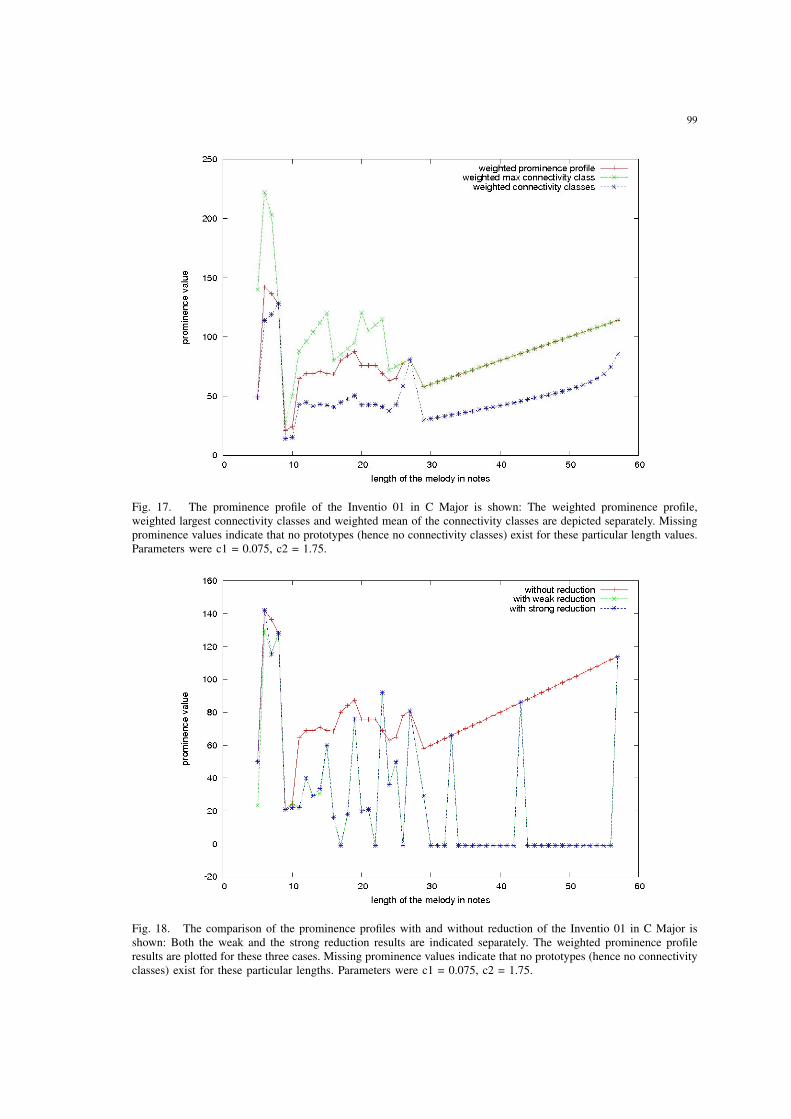
99

Fig. 17. The prominence profile of the Inventio 01 in C Major is shown: The weighted prominence profile,weighted largest connectivity classes and weighted mean of the connectivity classes are depicted separately. Missingprominence values indicate that no prototypes (hence no connectivity classes) exist for these particular length values.Parameters were c1 = 0.075, c2 = 1.75.

Fig. 18. The comparison of the prominence profiles with and without reduction of the Inventio 01 in C Major isshown: Both the weak and the strong reduction results are indicated separately. The weighted prominence profileresults are plotted for these three cases. Missing prominence values indicate that no prototypes (hence no connectivityclasses) exist for these particular lengths. Parameters were c1 = 0.075, c2 = 1.75.

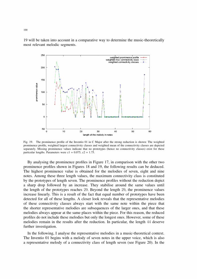
100

19 will be taken into account in a comparative way to determine the music-theoreticallymost relevant melodic segments.

Fig. 19. The prominence profile of the Inventio 01 in C Major after the strong reduction is shown: The weightedprominence profile, weighted largest connectivity classes and weighted mean of the connectivity classes are depictedseparately. Missing prominence values indicate that no prototypes (hence no connectivity classes) exist for theseparticular lengths. Parameters were c1 = 0.075, c2 = 1.75.

By analysing the prominence profiles in Figure 17, in comparison with the other twoprominence profiles shown in Figures 18 and 19, the following results can be deduced.The highest prominence value is obtained for the melodies of seven, eight and ninenotes. Among these three length values, the maximum connectivity class is constitutedby the prototypes of length seven. The prominence profiles without the reduction depicta sharp drop followed by an increase. They stabilise around the same values untilthe length of the prototypes reaches 29. Beyond the length 29, the prominence valuesincrease linearly. This is a result of the fact that equal number of prototypes have beendetected for all of these lengths. A closer look reveals that the representative melodiesof these connectivity classes always start with the same note within the piece thatthe shorter representative melodies are subsequences of the larger ones, and that thesemelodies always appear at the same places within the piece. For this reason, the reducedprofiles do not include these melodies but only the longest ones. However, some of thesemelodies remain in the results after the reduction. In particular, the length 44 deservefurther investigation.

In the following, I analyse the representative melodies in a music-theoretical context.The Inventio 01 begins with a melody of seven notes in the upper voice, which is alsoa representative melody of a connectivity class of length seven (see Figure 20). In the

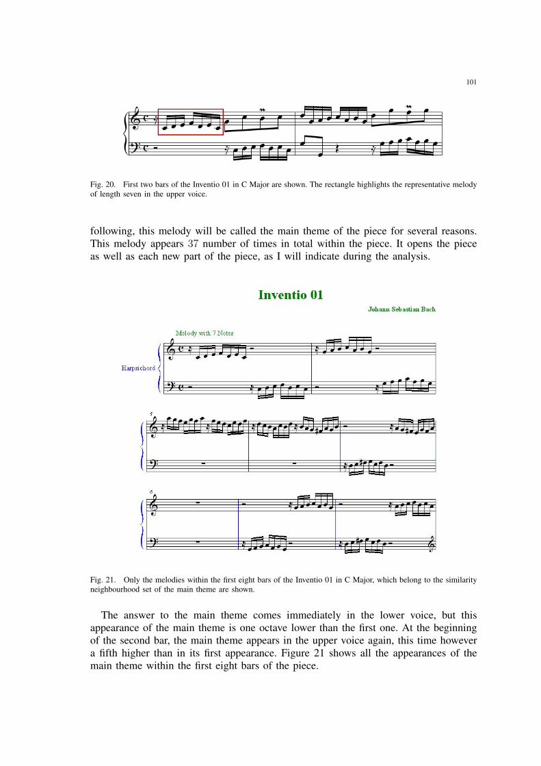
101

Fig. 20. First two bars of the Inventio 01 in C Major are shown. The rectangle highlights the representative melodyof length seven in the upper voice.

following, this melody will be called the main theme of the piece for several reasons.This melody appears 37 number of times in total within the piece. It opens the pieceas well as each new part of the piece, as I will indicate during the analysis.

Fig. 21. Only the melodies within the first eight bars of the Inventio 01 in C Major, which belong to the similarityneighbourhood set of the main theme are shown.

The answer to the main theme comes immediately in the lower voice, but thisappearance of the main theme is one octave lower than the first one. At the beginningof the second bar, the main theme appears in the upper voice again, this time howevera fifth higher than in its first appearance. Figure 21 shows all the appearances of themain theme within the first eight bars of the piece.

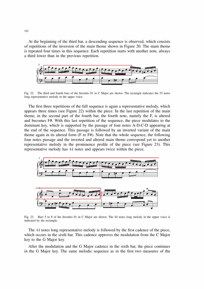
102

At the beginning of the third bar, a descending sequence is observed, which consistsof repetitions of the inversion of the main theme shown in Figure 20. The main themeis repeated four times in this sequence. Each repetition starts with another note, alwaysa third lower than in the previous repetition.

Fig. 22. The third and fourth bars of the Inventio 01 in C Major are shown. The rectangle indicates the 25 noteslong representative melody in the upper voice.

The first three repetitions of the full sequence is again a representative melody, whichappears three times (see Figure 22) within the piece. In the last repetition of the maintheme, in the second part of the fourth bar, the fourth note, namely the F, is alteredand becomes F#. With this last repetition of the sequence, the piece modulates to thedominant key, which is supported by the passage of four notes A-D-C-D appearing atthe end of the sequence. This passage is followed by an inverted variant of the maintheme again in its altered form (F to F#). Note that the whole sequence, the followingfour notes passage and the inverted and altered main theme correspond yet to anotherrepresentative melody in the prominence profile of the piece (see Figure 23). Thisrepresentative melody has 44 notes and appears twice within the piece.

Fig. 23. Bars 5 to 8 of the Inventio 01 in C Major are shown. The 44 notes long melody in the upper voice isindicated by the rectangle.

The 44 notes long representative melody is followed by the first cadence of the piece,which occurs in the sixth bar. This cadence approves the modulation from the C Majorkey to the G Major key.

After the modulation and the G Major cadence in the sixth bar, the piece continuesin the G Major key. The same melodic sequence as in the first two measures of the

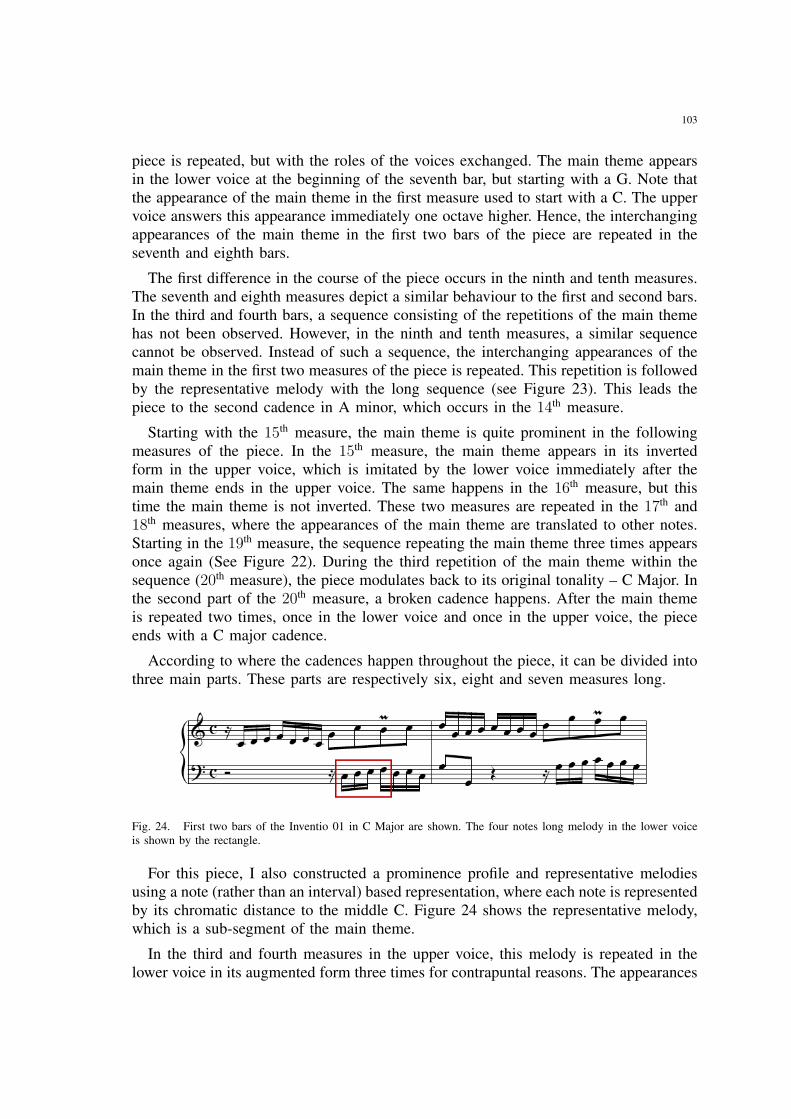
103

piece is repeated, but with the roles of the voices exchanged. The main theme appearsin the lower voice at the beginning of the seventh bar, but starting with a G. Note thatthe appearance of the main theme in the first measure used to start with a C. The uppervoice answers this appearance immediately one octave higher. Hence, the interchangingappearances of the main theme in the first two bars of the piece are repeated in theseventh and eighth bars.

The first difference in the course of the piece occurs in the ninth and tenth measures.The seventh and eighth measures depict a similar behaviour to the first and second bars.In the third and fourth bars, a sequence consisting of the repetitions of the main themehas not been observed. However, in the ninth and tenth measures, a similar sequencecannot be observed. Instead of such a sequence, the interchanging appearances of themain theme in the first two measures of the piece is repeated. This repetition is followedby the representative melody with the long sequence (see Figure 23). This leads thepiece to the second cadence in A minor, which occurs in the 14th measure.

Starting with the 15th measure, the main theme is quite prominent in the followingmeasures of the piece. In the 15th measure, the main theme appears in its invertedform in the upper voice, which is imitated by the lower voice immediately after themain theme ends in the upper voice. The same happens in the 16th measure, but thistime the main theme is not inverted. These two measures are repeated in the 17th and18th measures, where the appearances of the main theme are translated to other notes.Starting in the 19th measure, the sequence repeating the main theme three times appearsonce again (See Figure 22). During the third repetition of the main theme within thesequence (20th measure), the piece modulates back to its original tonality – C Major. Inthe second part of the 20th measure, a broken cadence happens. After the main themeis repeated two times, once in the lower voice and once in the upper voice, the pieceends with a C major cadence.

According to where the cadences happen throughout the piece, it can be divided intothree main parts. These parts are respectively six, eight and seven measures long.

Fig. 24. First two bars of the Inventio 01 in C Major are shown. The four notes long melody in the lower voiceis shown by the rectangle.

For this piece, I also constructed a prominence profile and representative melodiesusing a note (rather than an interval) based representation, where each note is representedby its chromatic distance to the middle C. Figure 24 shows the representative melody,which is a sub-segment of the main theme.

In the third and fourth measures in the upper voice, this melody is repeated in thelower voice in its augmented form three times for contrapuntal reasons. The appearances

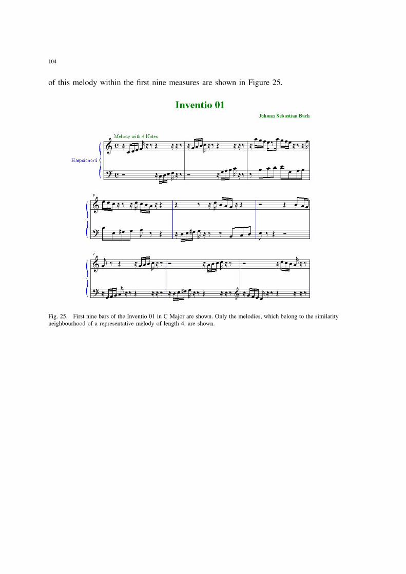
104

of this melody within the first nine measures are shown in Figure 25.

Fig. 25. First nine bars of the Inventio 01 in C Major are shown. Only the melodies, which belong to the similarityneighbourhood of a representative melody of length 4, are shown.

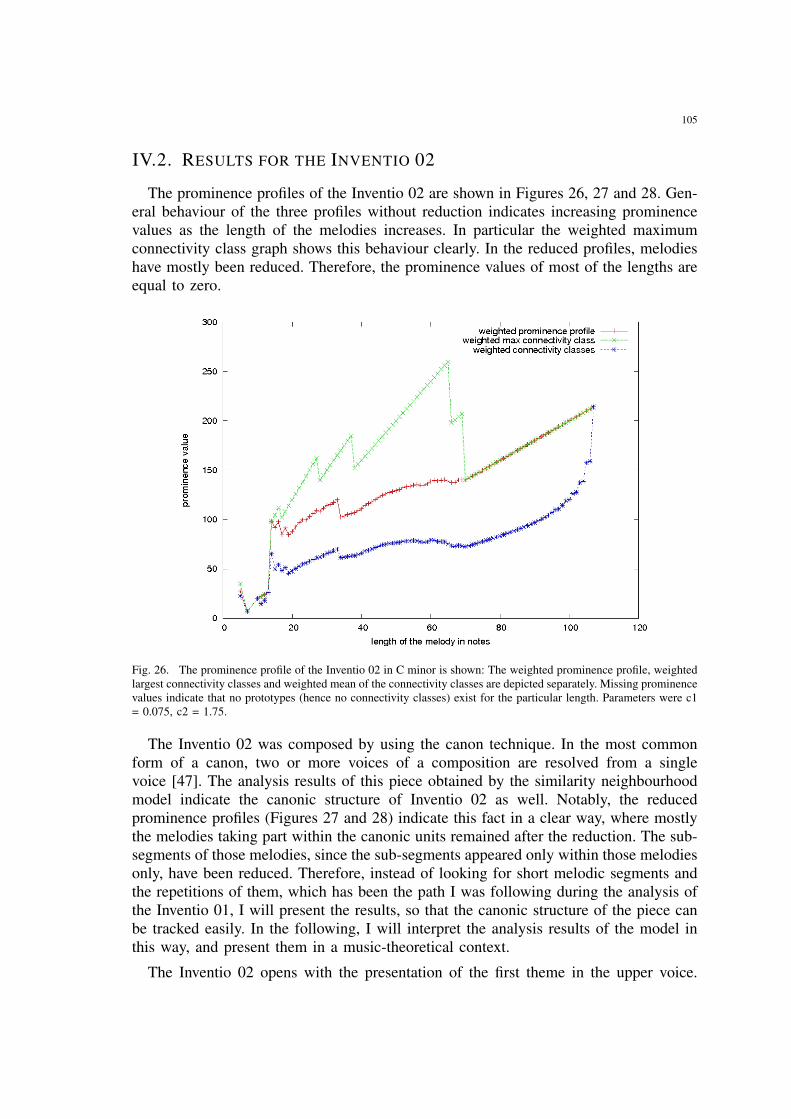
105

IV.2. RESULTS FOR THE INVENTIO 02

The prominence profiles of the Inventio 02 are shown in Figures 26, 27 and 28. Gen-eral behaviour of the three profiles without reduction indicates increasing prominencevalues as the length of the melodies increases. In particular the weighted maximumconnectivity class graph shows this behaviour clearly. In the reduced profiles, melodieshave mostly been reduced. Therefore, the prominence values of most of the lengths areequal to zero.

Fig. 26. The prominence profile of the Inventio 02 in C minor is shown: The weighted prominence profile, weightedlargest connectivity classes and weighted mean of the connectivity classes are depicted separately. Missing prominencevalues indicate that no prototypes (hence no connectivity classes) exist for the particular length. Parameters were c1= 0.075, c2 = 1.75.

The Inventio 02 was composed by using the canon technique. In the most commonform of a canon, two or more voices of a composition are resolved from a singlevoice [47]. The analysis results of this piece obtained by the similarity neighbourhoodmodel indicate the canonic structure of Inventio 02 as well. Notably, the reducedprominence profiles (Figures 27 and 28) indicate this fact in a clear way, where mostlythe melodies taking part within the canonic units remained after the reduction. The sub-segments of those melodies, since the sub-segments appeared only within those melodiesonly, have been reduced. Therefore, instead of looking for short melodic segments andthe repetitions of them, which has been the path I was following during the analysis ofthe Inventio 01, I will present the results, so that the canonic structure of the piece canbe tracked easily. In the following, I will interpret the analysis results of the model inthis way, and present them in a music-theoretical context.

The Inventio 02 opens with the presentation of the first theme in the upper voice.

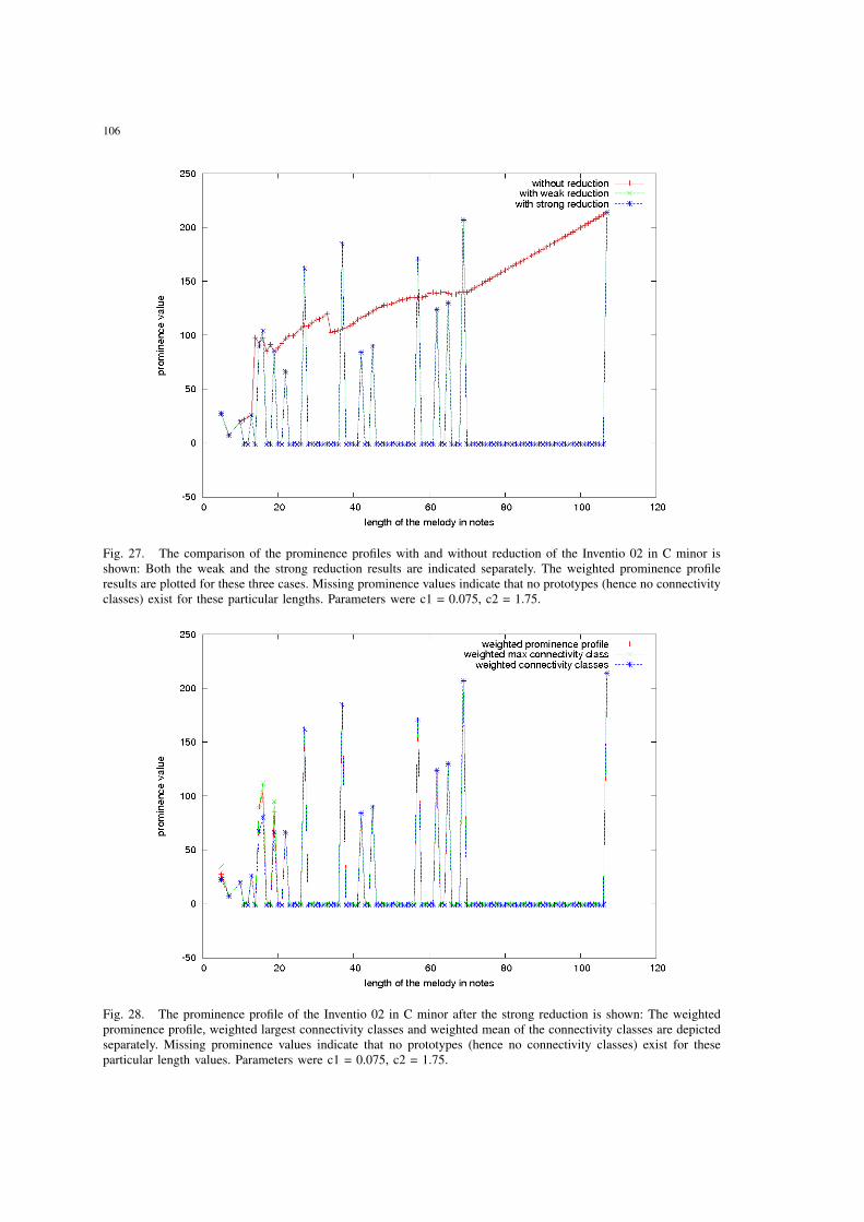
106

Fig. 27. The comparison of the prominence profiles with and without reduction of the Inventio 02 in C minor isshown: Both the weak and the strong reduction results are indicated separately. The weighted prominence profileresults are plotted for these three cases. Missing prominence values indicate that no prototypes (hence no connectivityclasses) exist for these particular lengths. Parameters were c1 = 0.075, c2 = 1.75.

Fig. 28. The prominence profile of the Inventio 02 in C minor after the strong reduction is shown: The weightedprominence profile, weighted largest connectivity classes and weighted mean of the connectivity classes are depictedseparately. Missing prominence values indicate that no prototypes (hence no connectivity classes) exist for theseparticular length values. Parameters were c1 = 0.075, c2 = 1.75.

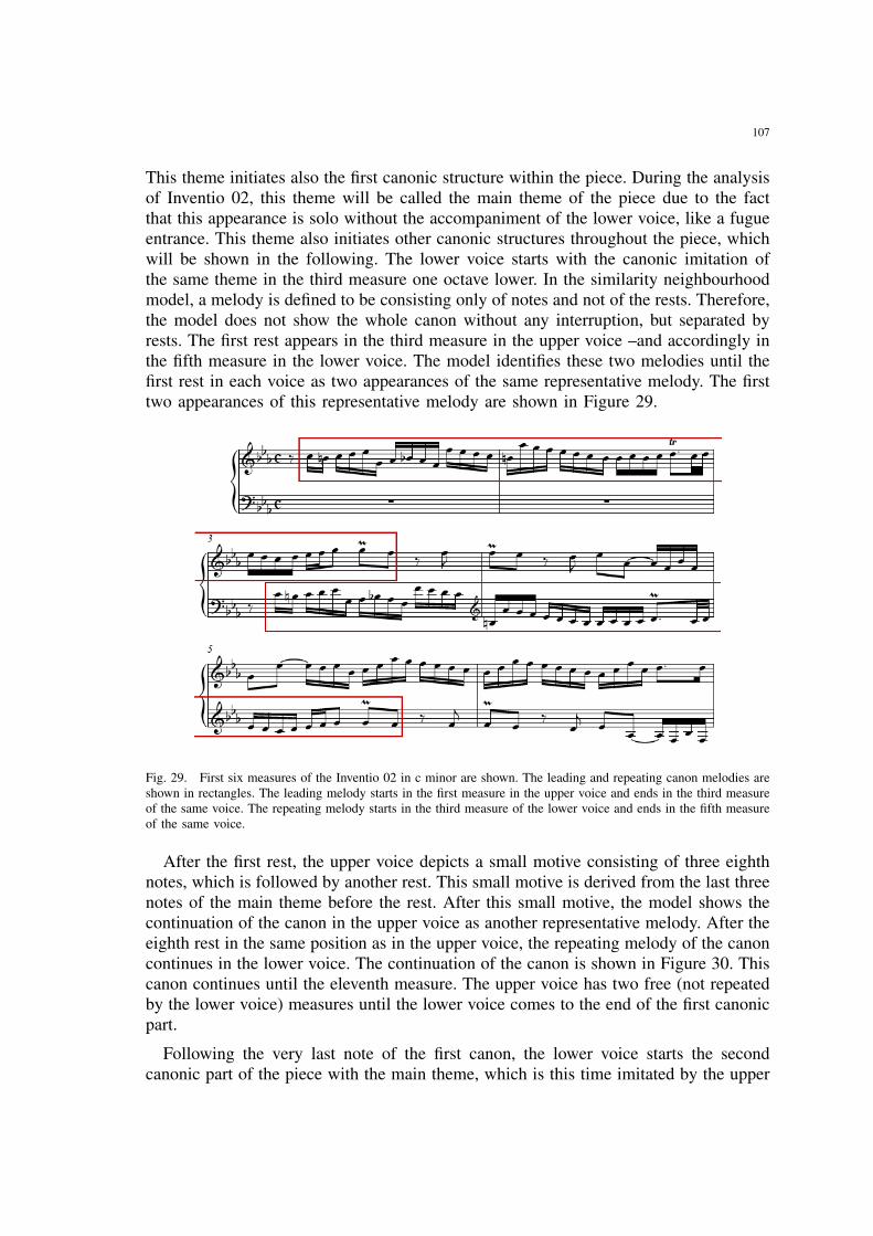
107

This theme initiates also the first canonic structure within the piece. During the analysisof Inventio 02, this theme will be called the main theme of the piece due to the factthat this appearance is solo without the accompaniment of the lower voice, like a fugueentrance. This theme also initiates other canonic structures throughout the piece, whichwill be shown in the following. The lower voice starts with the canonic imitation ofthe same theme in the third measure one octave lower. In the similarity neighbourhoodmodel, a melody is defined to be consisting only of notes and not of the rests. Therefore,the model does not show the whole canon without any interruption, but separated byrests. The first rest appears in the third measure in the upper voice –and accordingly inthe fifth measure in the lower voice. The model identifies these two melodies until thefirst rest in each voice as two appearances of the same representative melody. The firsttwo appearances of this representative melody are shown in Figure 29.

Fig. 29. First six measures of the Inventio 02 in c minor are shown. The leading and repeating canon melodies areshown in rectangles. The leading melody starts in the first measure in the upper voice and ends in the third measureof the same voice. The repeating melody starts in the third measure of the lower voice and ends in the fifth measureof the same voice.

After the first rest, the upper voice depicts a small motive consisting of three eighthnotes, which is followed by another rest. This small motive is derived from the last threenotes of the main theme before the rest. After this small motive, the model shows thecontinuation of the canon in the upper voice as another representative melody. After theeighth rest in the same position as in the upper voice, the repeating melody of the canoncontinues in the lower voice. The continuation of the canon is shown in Figure 30. Thiscanon continues until the eleventh measure. The upper voice has two free (not repeatedby the lower voice) measures until the lower voice comes to the end of the first canonicpart.

Following the very last note of the first canon, the lower voice starts the secondcanonic part of the piece with the main theme, which is this time imitated by the upper

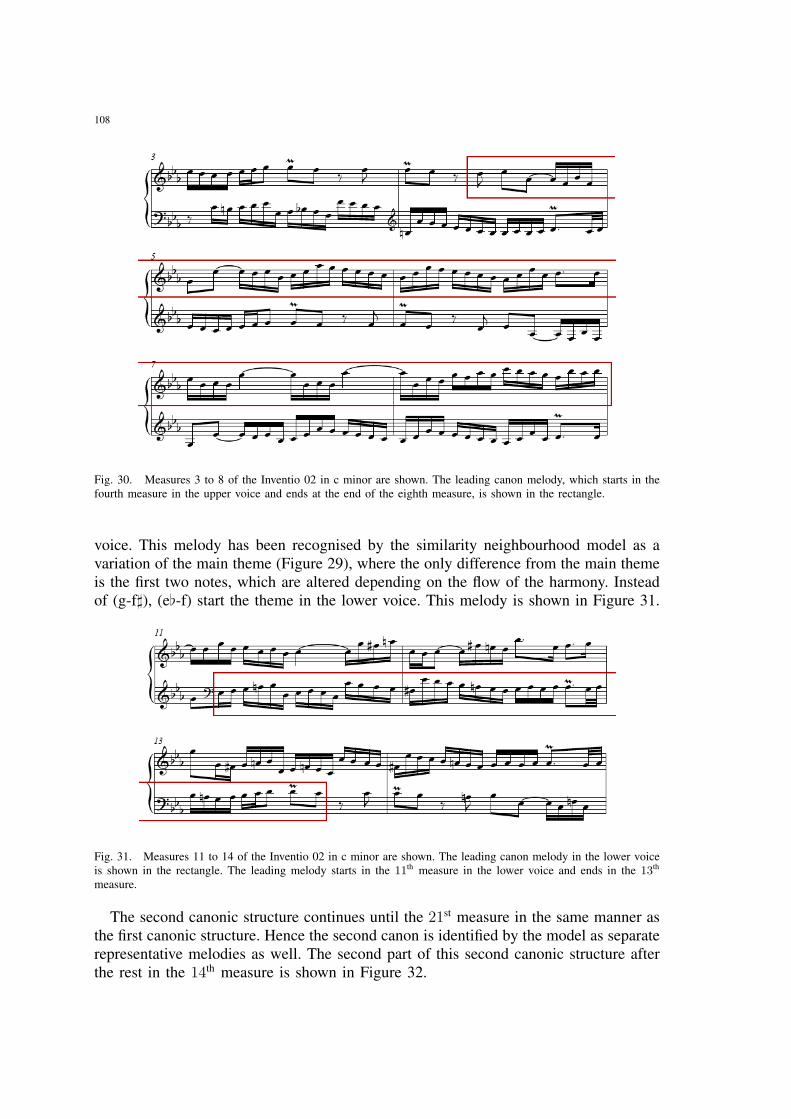
108

Fig. 30. Measures 3 to 8 of the Inventio 02 in c minor are shown. The leading canon melody, which starts in thefourth measure in the upper voice and ends at the end of the eighth measure, is shown in the rectangle.

voice. This melody has been recognised by the similarity neighbourhood model as avariation of the main theme (Figure 29), where the only difference from the main themeis the first two notes, which are altered depending on the flow of the harmony. Insteadof (g-f]), (e[-f) start the theme in the lower voice. This melody is shown in Figure 31.

Fig. 31. Measures 11 to 14 of the Inventio 02 in c minor are shown. The leading canon melody in the lower voiceis shown in the rectangle. The leading melody starts in the 11th measure in the lower voice and ends in the 13th

measure.

The second canonic structure continues until the 21st measure in the same manner asthe first canonic structure. Hence the second canon is identified by the model as separaterepresentative melodies as well. The second part of this second canonic structure afterthe rest in the 14th measure is shown in Figure 32.

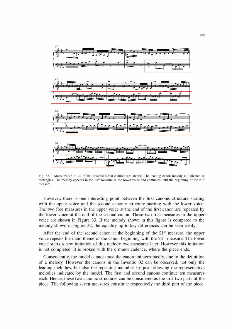
109

Fig. 32. Measures 13 to 22 of the Inventio 02 in c minor are shown. The leading canon melody is indicated inrectangles. The melody appears in the 14th measure in the lower voice and continues until the beginning of the 21st

measure.

However, there is one interesting point between the first canonic structure startingwith the upper voice and the second canonic structure starting with the lower voice.The two free measures in the upper voice at the end of the first canon are repeated bythe lower voice at the end of the second canon. These two free measures in the uppervoice are shown in Figure 33. If the melody shown in this figure is compared to themelody shown in Figure 32, the equality up to key differences can be seen easily.

After the end of the second canon at the beginning of the 21st measure, the uppervoice repeats the main theme of the canon beginning with the 23rd measure. The lowervoice starts a new imitation of this melody two measures later. However this imitationis not completed. It is broken with the c minor cadence, where the piece ends.

Consequently, the model cannot trace the canon uninterruptedly, due to the definitionof a melody. However the canons in the Inventio 02 can be observed, not only theleading melodies, but also the repeating melodies by just following the representativemelodies indicated by the model. The first and second canons continue ten measureseach. Hence, these two canonic structures can be considered as the first two parts of thepiece. The following seven measures constitute respectively the third part of the piece.

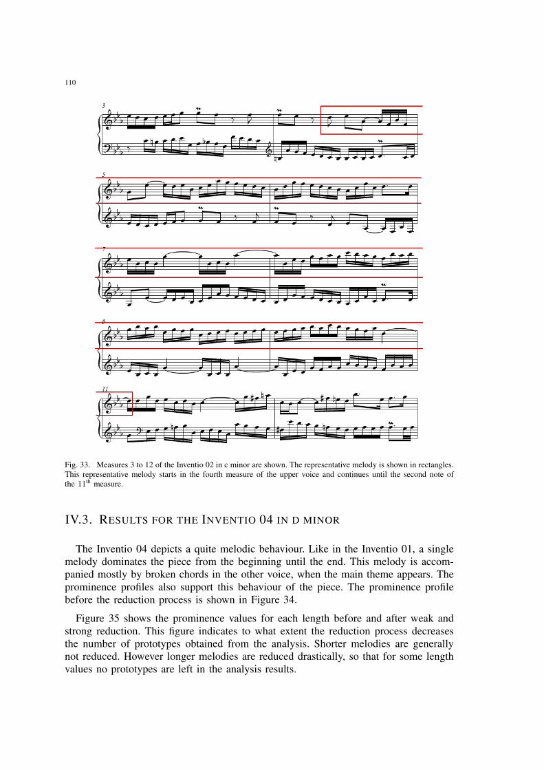
110

Fig. 33. Measures 3 to 12 of the Inventio 02 in c minor are shown. The representative melody is shown in rectangles.This representative melody starts in the fourth measure of the upper voice and continues until the second note ofthe 11th measure.

IV.3. RESULTS FOR THE INVENTIO 04 IN D MINOR

The Inventio 04 depicts a quite melodic behaviour. Like in the Inventio 01, a singlemelody dominates the piece from the beginning until the end. This melody is accom-panied mostly by broken chords in the other voice, when the main theme appears. Theprominence profiles also support this behaviour of the piece. The prominence profilebefore the reduction process is shown in Figure 34.

Figure 35 shows the prominence values for each length before and after weak andstrong reduction. This figure indicates to what extent the reduction process decreasesthe number of prototypes obtained from the analysis. Shorter melodies are generallynot reduced. However longer melodies are reduced drastically, so that for some lengthvalues no prototypes are left in the analysis results.

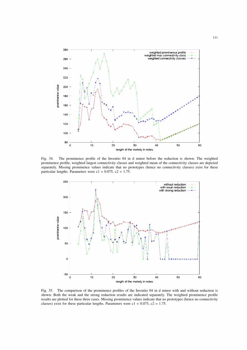
111

Fig. 34. The prominence profile of the Inventio 04 in d minor before the reduction is shown: The weightedprominence profile, weighted largest connectivity classes and weighted mean of the connectivity classes are depictedseparately. Missing prominence values indicate that no prototypes (hence no connectivity classes) exist for theseparticular lengths. Parameters were c1 = 0.075, c2 = 1.75.

Fig. 35. The comparison of the prominence profiles of the Inventio 04 in d minor with and without reduction isshown: Both the weak and the strong reduction results are indicated separately. The weighted prominence profileresults are plotted for these three cases. Missing prominence values indicate that no prototypes (hence no connectivityclasses) exist for these particular lengths. Parameters were c1 = 0.075, c2 = 1.75.

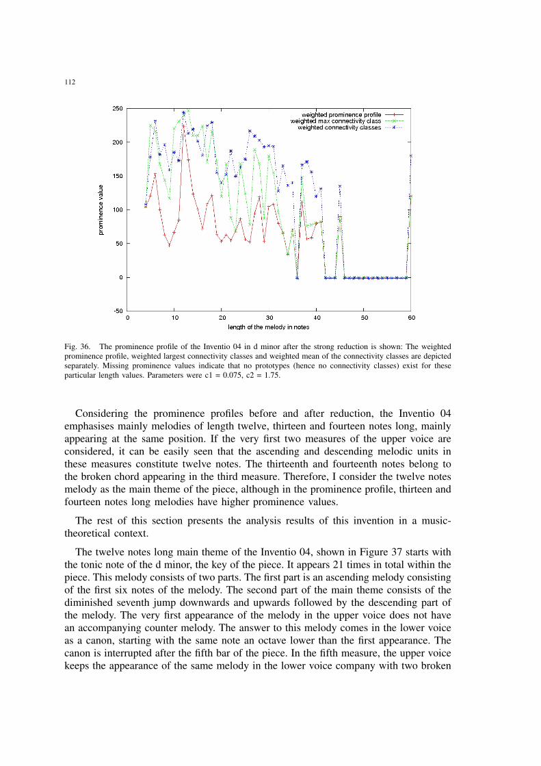
112

Fig. 36. The prominence profile of the Inventio 04 in d minor after the strong reduction is shown: The weightedprominence profile, weighted largest connectivity classes and weighted mean of the connectivity classes are depictedseparately. Missing prominence values indicate that no prototypes (hence no connectivity classes) exist for theseparticular length values. Parameters were c1 = 0.075, c2 = 1.75.

Considering the prominence profiles before and after reduction, the Inventio 04emphasises mainly melodies of length twelve, thirteen and fourteen notes long, mainlyappearing at the same position. If the very first two measures of the upper voice areconsidered, it can be easily seen that the ascending and descending melodic units inthese measures constitute twelve notes. The thirteenth and fourteenth notes belong tothe broken chord appearing in the third measure. Therefore, I consider the twelve notesmelody as the main theme of the piece, although in the prominence profile, thirteen andfourteen notes long melodies have higher prominence values.

The rest of this section presents the analysis results of this invention in a music-theoretical context.

The twelve notes long main theme of the Inventio 04, shown in Figure 37 starts withthe tonic note of the d minor, the key of the piece. It appears 21 times in total within thepiece. This melody consists of two parts. The first part is an ascending melody consistingof the first six notes of the melody. The second part of the main theme consists of thediminished seventh jump downwards and upwards followed by the descending part ofthe melody. The very first appearance of the melody in the upper voice does not havean accompanying counter melody. The answer to this melody comes in the lower voiceas a canon, starting with the same note an octave lower than the first appearance. Thecanon is interrupted after the fifth bar of the piece. In the fifth measure, the upper voicekeeps the appearance of the same melody in the lower voice company with two broken

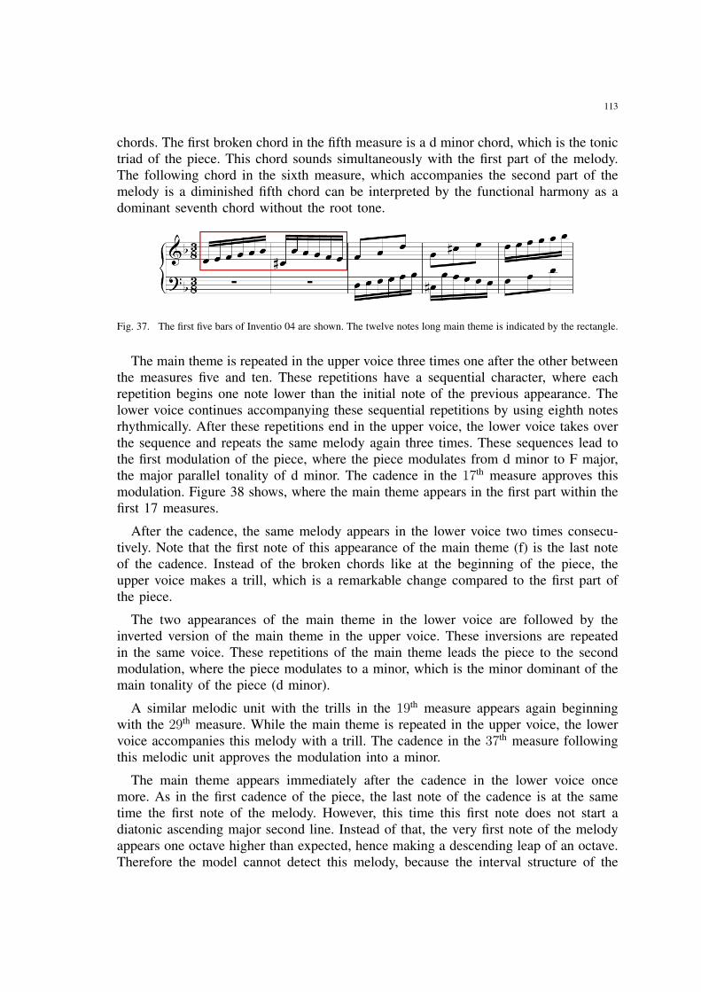
113

chords. The first broken chord in the fifth measure is a d minor chord, which is the tonictriad of the piece. This chord sounds simultaneously with the first part of the melody.The following chord in the sixth measure, which accompanies the second part of themelody is a diminished fifth chord can be interpreted by the functional harmony as adominant seventh chord without the root tone.

Fig. 37. The first five bars of Inventio 04 are shown. The twelve notes long main theme is indicated by the rectangle.

The main theme is repeated in the upper voice three times one after the other betweenthe measures five and ten. These repetitions have a sequential character, where eachrepetition begins one note lower than the initial note of the previous appearance. Thelower voice continues accompanying these sequential repetitions by using eighth notesrhythmically. After these repetitions end in the upper voice, the lower voice takes overthe sequence and repeats the same melody again three times. These sequences lead tothe first modulation of the piece, where the piece modulates from d minor to F major,the major parallel tonality of d minor. The cadence in the 17th measure approves thismodulation. Figure 38 shows, where the main theme appears in the first part within thefirst 17 measures.

After the cadence, the same melody appears in the lower voice two times consecu-tively. Note that the first note of this appearance of the main theme (f) is the last noteof the cadence. Instead of the broken chords like at the beginning of the piece, theupper voice makes a trill, which is a remarkable change compared to the first part ofthe piece.

The two appearances of the main theme in the lower voice are followed by theinverted version of the main theme in the upper voice. These inversions are repeatedin the same voice. These repetitions of the main theme leads the piece to the secondmodulation, where the piece modulates to a minor, which is the minor dominant of themain tonality of the piece (d minor).

A similar melodic unit with the trills in the 19th measure appears again beginningwith the 29th measure. While the main theme is repeated in the upper voice, the lowervoice accompanies this melody with a trill. The cadence in the 37th measure followingthis melodic unit approves the modulation into a minor.

The main theme appears immediately after the cadence in the lower voice oncemore. As in the first cadence of the piece, the last note of the cadence is at the sametime the first note of the melody. However, this time this first note does not start adiatonic ascending major second line. Instead of that, the very first note of the melodyappears one octave higher than expected, hence making a descending leap of an octave.Therefore the model cannot detect this melody, because the interval structure of the

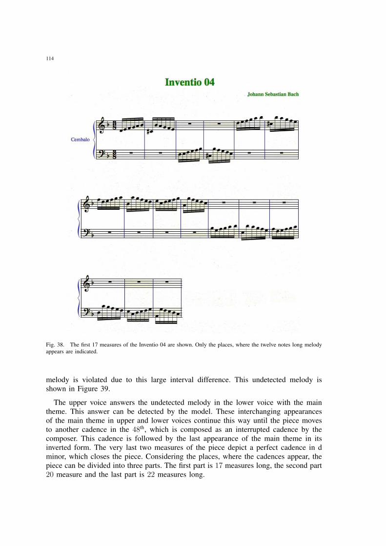
114

Fig. 38. The first 17 measures of the Inventio 04 are shown. Only the places, where the twelve notes long melodyappears are indicated.

melody is violated due to this large interval difference. This undetected melody isshown in Figure 39.

The upper voice answers the undetected melody in the lower voice with the maintheme. This answer can be detected by the model. These interchanging appearancesof the main theme in upper and lower voices continue this way until the piece movesto another cadence in the 48th, which is composed as an interrupted cadence by thecomposer. This cadence is followed by the last appearance of the main theme in itsinverted form. The very last two measures of the piece depict a perfect cadence in dminor, which closes the piece. Considering the places, where the cadences appear, thepiece can be divided into three parts. The first part is 17 measures long, the second part20 measure and the last part is 22 measures long.

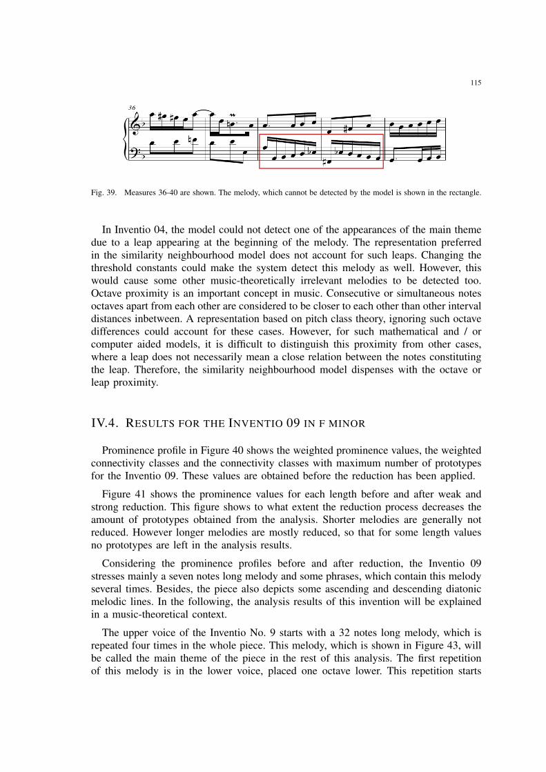
115

Fig. 39. Measures 36-40 are shown. The melody, which cannot be detected by the model is shown in the rectangle.

In Inventio 04, the model could not detect one of the appearances of the main themedue to a leap appearing at the beginning of the melody. The representation preferredin the similarity neighbourhood model does not account for such leaps. Changing thethreshold constants could make the system detect this melody as well. However, thiswould cause some other music-theoretically irrelevant melodies to be detected too.Octave proximity is an important concept in music. Consecutive or simultaneous notesoctaves apart from each other are considered to be closer to each other than other intervaldistances inbetween. A representation based on pitch class theory, ignoring such octavedifferences could account for these cases. However, for such mathematical and / orcomputer aided models, it is difficult to distinguish this proximity from other cases,where a leap does not necessarily mean a close relation between the notes constitutingthe leap. Therefore, the similarity neighbourhood model dispenses with the octave orleap proximity.

IV.4. RESULTS FOR THE INVENTIO 09 IN F MINOR

Prominence profile in Figure 40 shows the weighted prominence values, the weightedconnectivity classes and the connectivity classes with maximum number of prototypesfor the Inventio 09. These values are obtained before the reduction has been applied.

Figure 41 shows the prominence values for each length before and after weak andstrong reduction. This figure shows to what extent the reduction process decreases theamount of prototypes obtained from the analysis. Shorter melodies are generally notreduced. However longer melodies are mostly reduced, so that for some length valuesno prototypes are left in the analysis results.

Considering the prominence profiles before and after reduction, the Inventio 09stresses mainly a seven notes long melody and some phrases, which contain this melodyseveral times. Besides, the piece also depicts some ascending and descending diatonicmelodic lines. In the following, the analysis results of this invention will be explainedin a music-theoretical context.

The upper voice of the Inventio No. 9 starts with a 32 notes long melody, which isrepeated four times in the whole piece. This melody, which is shown in Figure 43, willbe called the main theme of the piece in the rest of this analysis. The first repetitionof this melody is in the lower voice, placed one octave lower. This repetition starts

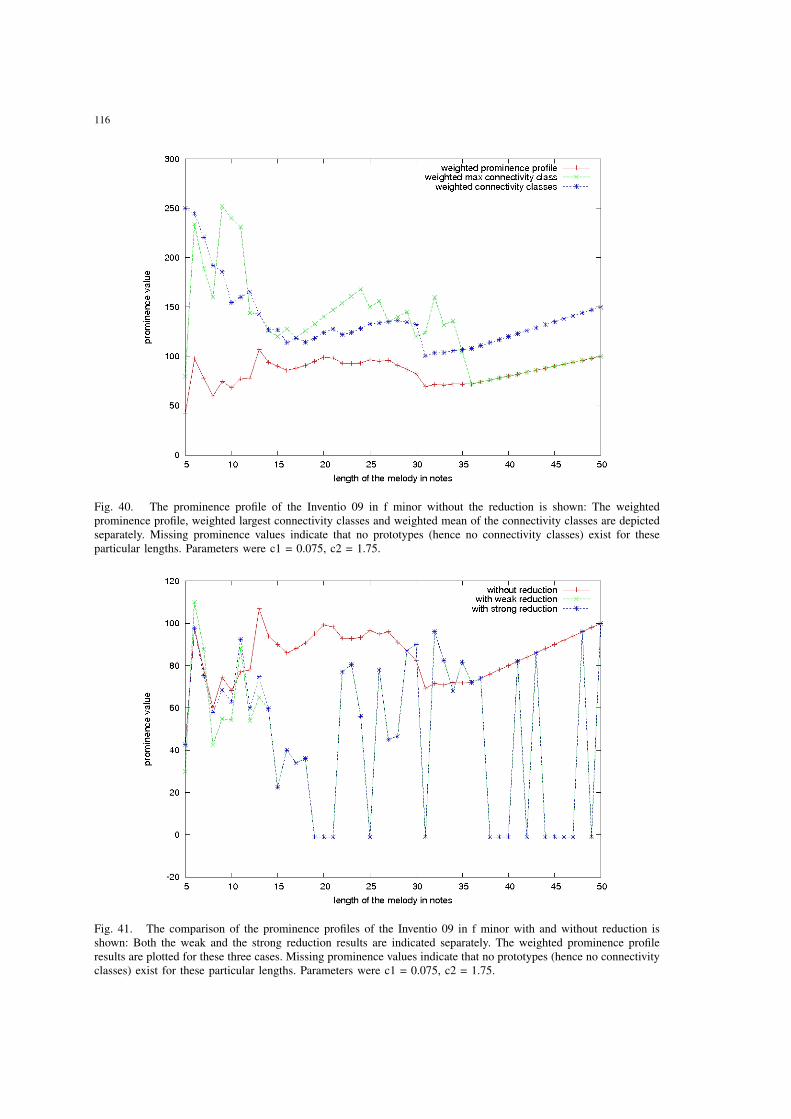
116

Fig. 40. The prominence profile of the Inventio 09 in f minor without the reduction is shown: The weightedprominence profile, weighted largest connectivity classes and weighted mean of the connectivity classes are depictedseparately. Missing prominence values indicate that no prototypes (hence no connectivity classes) exist for theseparticular lengths. Parameters were c1 = 0.075, c2 = 1.75.

Fig. 41. The comparison of the prominence profiles of the Inventio 09 in f minor with and without reduction isshown: Both the weak and the strong reduction results are indicated separately. The weighted prominence profileresults are plotted for these three cases. Missing prominence values indicate that no prototypes (hence no connectivityclasses) exist for these particular lengths. Parameters were c1 = 0.075, c2 = 1.75.

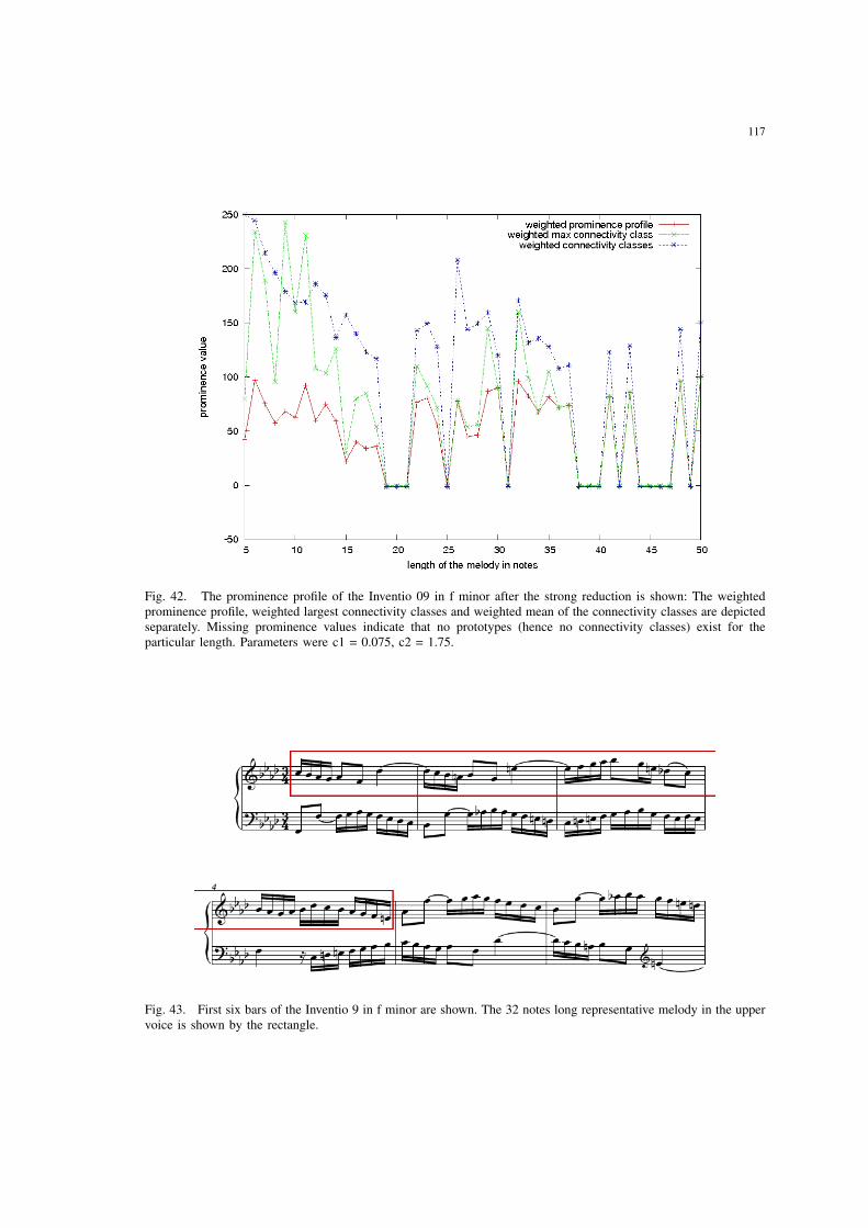
117

Fig. 42. The prominence profile of the Inventio 09 in f minor after the strong reduction is shown: The weightedprominence profile, weighted largest connectivity classes and weighted mean of the connectivity classes are depictedseparately. Missing prominence values indicate that no prototypes (hence no connectivity classes) exist for theparticular length. Parameters were c1 = 0.075, c2 = 1.75.

Fig. 43. First six bars of the Inventio 9 in f minor are shown. The 32 notes long representative melody in the uppervoice is shown by the rectangle.

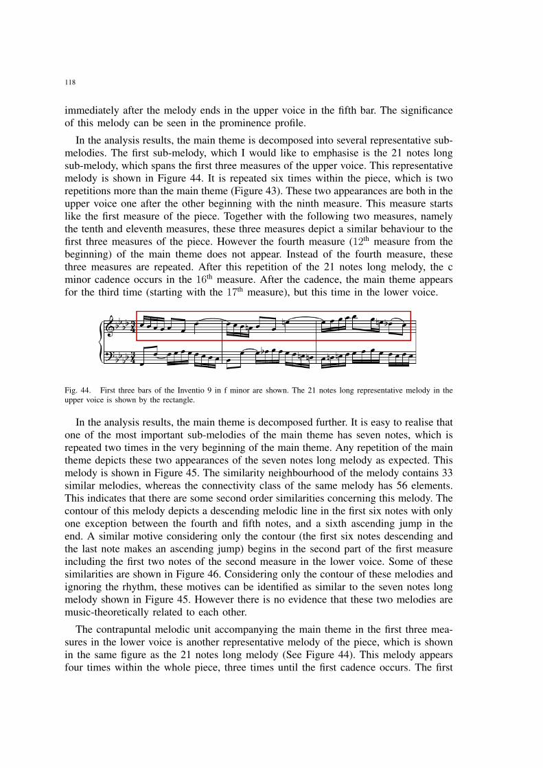
118

immediately after the melody ends in the upper voice in the fifth bar. The significanceof this melody can be seen in the prominence profile.

In the analysis results, the main theme is decomposed into several representative sub-melodies. The first sub-melody, which I would like to emphasise is the 21 notes longsub-melody, which spans the first three measures of the upper voice. This representativemelody is shown in Figure 44. It is repeated six times within the piece, which is tworepetitions more than the main theme (Figure 43). These two appearances are both in theupper voice one after the other beginning with the ninth measure. This measure startslike the first measure of the piece. Together with the following two measures, namelythe tenth and eleventh measures, these three measures depict a similar behaviour to thefirst three measures of the piece. However the fourth measure (12th measure from thebeginning) of the main theme does not appear. Instead of the fourth measure, thesethree measures are repeated. After this repetition of the 21 notes long melody, the cminor cadence occurs in the 16th measure. After the cadence, the main theme appearsfor the third time (starting with the 17th measure), but this time in the lower voice.

Fig. 44. First three bars of the Inventio 9 in f minor are shown. The 21 notes long representative melody in theupper voice is shown by the rectangle.

In the analysis results, the main theme is decomposed further. It is easy to realise thatone of the most important sub-melodies of the main theme has seven notes, which isrepeated two times in the very beginning of the main theme. Any repetition of the maintheme depicts these two appearances of the seven notes long melody as expected. Thismelody is shown in Figure 45. The similarity neighbourhood of the melody contains 33similar melodies, whereas the connectivity class of the same melody has 56 elements.This indicates that there are some second order similarities concerning this melody. Thecontour of this melody depicts a descending melodic line in the first six notes with onlyone exception between the fourth and fifth notes, and a sixth ascending jump in theend. A similar motive considering only the contour (the first six notes descending andthe last note makes an ascending jump) begins in the second part of the first measureincluding the first two notes of the second measure in the lower voice. Some of thesesimilarities are shown in Figure 46. Considering only the contour of these melodies andignoring the rhythm, these motives can be identified as similar to the seven notes longmelody shown in Figure 45. However there is no evidence that these two melodies aremusic-theoretically related to each other.

The contrapuntal melodic unit accompanying the main theme in the first three mea-sures in the lower voice is another representative melody of the piece, which is shownin the same figure as the 21 notes long melody (See Figure 44). This melody appearsfour times within the whole piece, three times until the first cadence occurs. The first

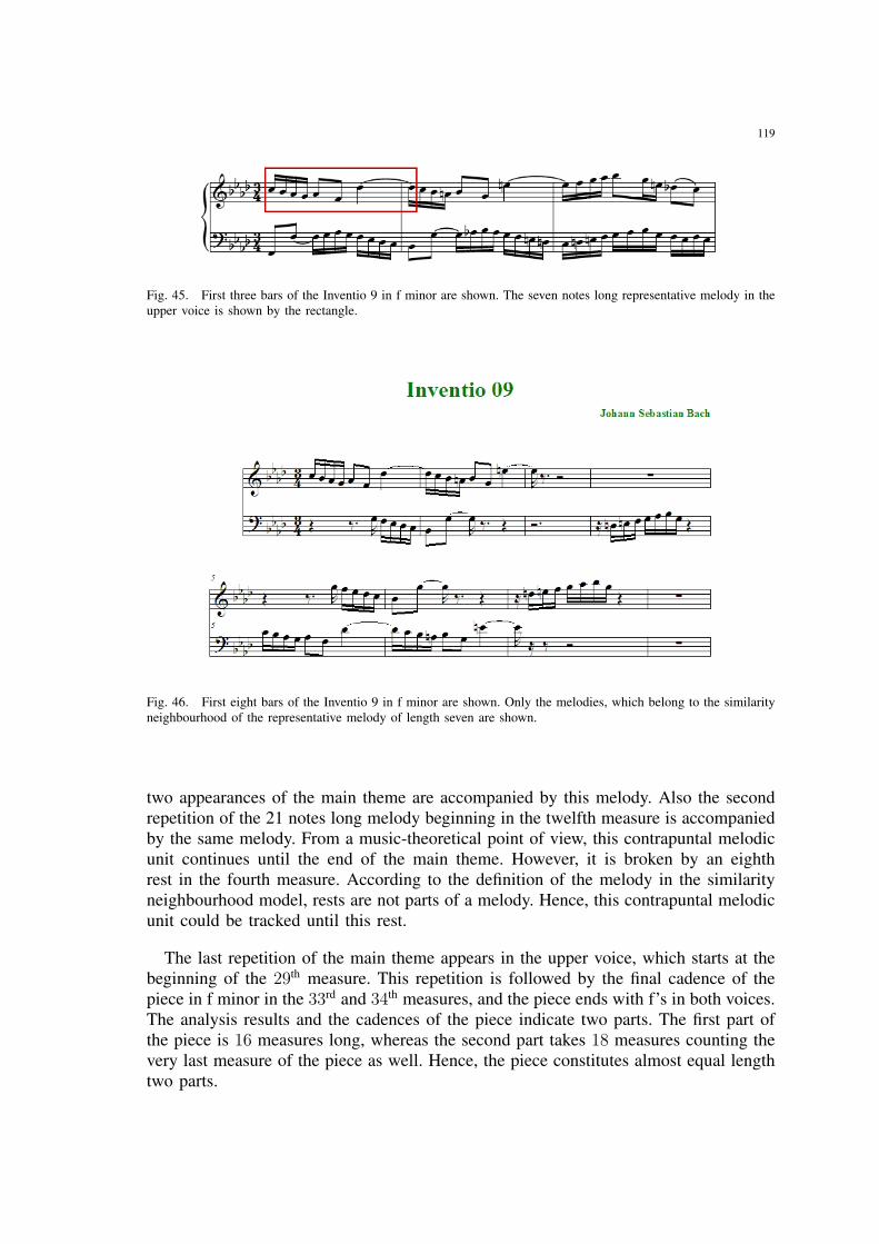
119

Fig. 45. First three bars of the Inventio 9 in f minor are shown. The seven notes long representative melody in theupper voice is shown by the rectangle.

Fig. 46. First eight bars of the Inventio 9 in f minor are shown. Only the melodies, which belong to the similarityneighbourhood of the representative melody of length seven are shown.

two appearances of the main theme are accompanied by this melody. Also the secondrepetition of the 21 notes long melody beginning in the twelfth measure is accompaniedby the same melody. From a music-theoretical point of view, this contrapuntal melodicunit continues until the end of the main theme. However, it is broken by an eighthrest in the fourth measure. According to the definition of the melody in the similarityneighbourhood model, rests are not parts of a melody. Hence, this contrapuntal melodicunit could be tracked until this rest.

The last repetition of the main theme appears in the upper voice, which starts at thebeginning of the 29th measure. This repetition is followed by the final cadence of thepiece in f minor in the 33rd and 34th measures, and the piece ends with f’s in both voices.The analysis results and the cadences of the piece indicate two parts. The first part ofthe piece is 16 measures long, whereas the second part takes 18 measures counting thevery last measure of the piece as well. Hence, the piece constitutes almost equal lengthtwo parts.

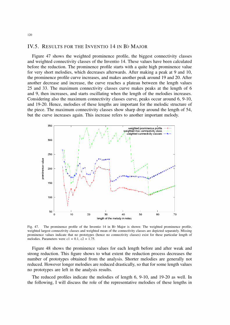
120

IV.5. RESULTS FOR THE INVENTIO 14 IN B[ MAJOR

Figure 47 shows the weighted prominence profile, the biggest connectivity classesand weighted connectivity classes of the Inventio 14. These values have been calculatedbefore the reduction. The prominence profile starts with a quite high prominence valuefor very short melodies, which decreases afterwards. After making a peak at 9 and 10,the prominence profile curve increases, and makes another peak around 19 and 20. Afteranother decrease and increase, the curve reaches a plateau between the length values25 and 33. The maximum connectivity classes curve makes peaks at the length of 6and 9, then increases, and starts oscillating when the length of the melodies increases.Considering also the maximum connectivity classes curve, peaks occur around 6, 9-10,and 19-20. Hence, melodies of these lengths are important for the melodic structure ofthe piece. The maximum connectivity classes show sharp drop around the length of 54,but the curve increases again. This increase refers to another important melody.

Fig. 47. The prominence profile of the Inventio 14 in B[ Major is shown: The weighted prominence profile,weighted largest connectivity classes and weighted mean of the connectivity classes are depicted separately. Missingprominence values indicate that no prototypes (hence no connectivity classes) exist for these particular length ofmelodies. Parameters were c1 = 0.1, c2 = 1.75.

Figure 48 shows the prominence values for each length before and after weak andstrong reduction. This figure shows to what extent the reduction process decreases thenumber of prototypes obtained from the analysis. Shorter melodies are generally notreduced. However longer melodies are reduced drastically, so that for some length valuesno prototypes are left in the analysis results.

The reduced profiles indicate the melodies of length 6, 9-10, and 19-20 as well. Inthe following, I will discuss the role of the representative melodies of these lengths in

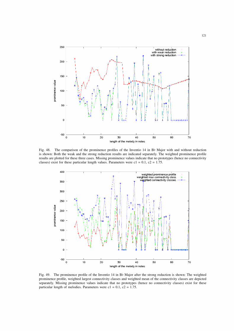
121

Fig. 48. The comparison of the prominence profiles of the Inventio 14 in B[ Major with and without reductionis shown: Both the weak and the strong reduction results are indicated separately. The weighted prominence profileresults are plotted for these three cases. Missing prominence values indicate that no prototypes (hence no connectivityclasses) exist for these particular length values. Parameters were c1 = 0.1, c2 = 1.75.

Fig. 49. The prominence profile of the Inventio 14 in B[ Major after the strong reduction is shown: The weightedprominence profile, weighted largest connectivity classes and weighted mean of the connectivity classes are depictedseparately. Missing prominence values indicate that no prototypes (hence no connectivity classes) exist for theseparticular length of melodies. Parameters were c1 = 0.1, c2 = 1.75.

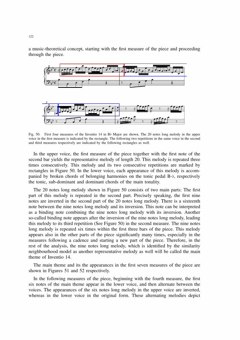
122

a music-theoretical concept, starting with the first measure of the piece and proceedingthrough the piece.

Fig. 50. First four measures of the Inventio 14 in B[ Major are shown. The 20 notes long melody in the uppervoice in the first measure is indicated by the rectangle. The following two repetitions in the same voice in the secondand third measures respectively are indicated by the following rectangles as well.

In the upper voice, the first measure of the piece together with the first note of thesecond bar yields the representative melody of length 20. This melody is repeated threetimes consecutively. This melody and its two consecutive repetitions are marked byrectangles in Figure 50. In the lower voice, each appearance of this melody is accom-panied by broken chords of belonging harmonies on the tonic pedal B-[, respectivelythe tonic, sub-dominant and dominant chords of the main tonality.

The 20 notes long melody shown in Figure 50 consists of two main parts: The firstpart of this melody is repeated in the second part. Precisely speaking, the first ninenotes are inverted in the second part of the 20 notes long melody. There is a sixteenthnote between the nine notes long melody and its inversion. This note can be interpretedas a binding note combining the nine notes long melody with its inversion. Anotherso-called binding note appears after the inversion of the nine notes long melody, leadingthis melody to its third repetition (See Figure 50) in the second measure. The nine noteslong melody is repeated six times within the first three bars of the piece. This melodyappears also in the other parts of the piece significantly many times, especially in themeasures following a cadence and starting a new part of the piece. Therefore, in therest of the analysis, the nine notes long melody, which is identified by the similarityneighbourhood model as another representative melody as well will be called the maintheme of Inventio 14.

The main theme and its the appearances in the first seven measures of the piece areshown in Figures 51 and 52 respectively.

In the following measures of the piece, beginning with the fourth measure, the firstsix notes of the main theme appear in the lower voice, and then alternate between thevoices. The appearances of the six notes long melody in the upper voice are inverted,whereas in the lower voice in the original form. These alternating melodies depict

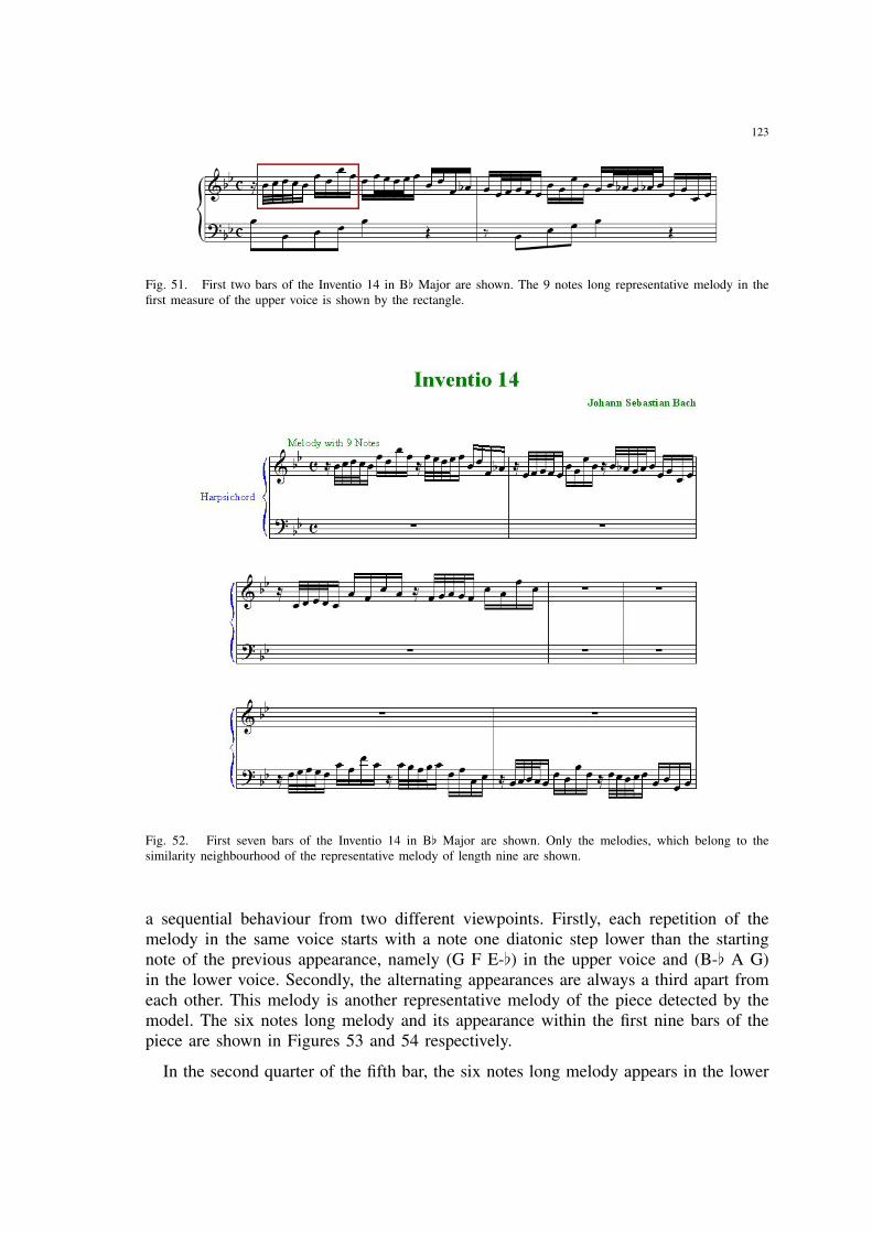
123

Fig. 51. First two bars of the Inventio 14 in B[ Major are shown. The 9 notes long representative melody in thefirst measure of the upper voice is shown by the rectangle.

Fig. 52. First seven bars of the Inventio 14 in B[ Major are shown. Only the melodies, which belong to thesimilarity neighbourhood of the representative melody of length nine are shown.

a sequential behaviour from two different viewpoints. Firstly, each repetition of themelody in the same voice starts with a note one diatonic step lower than the startingnote of the previous appearance, namely (G F E-[) in the upper voice and (B-[ A G)in the lower voice. Secondly, the alternating appearances are always a third apart fromeach other. This melody is another representative melody of the piece detected by themodel. The six notes long melody and its appearance within the first nine bars of thepiece are shown in Figures 53 and 54 respectively.

In the second quarter of the fifth bar, the six notes long melody appears in the lower

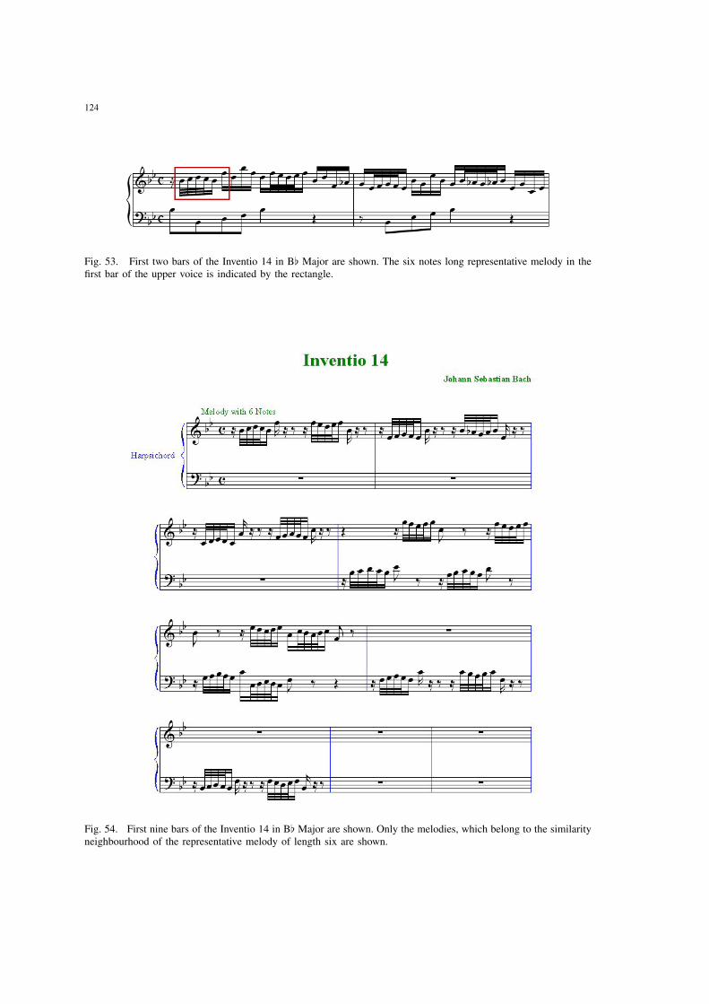
124

Fig. 53. First two bars of the Inventio 14 in B[ Major are shown. The six notes long representative melody in thefirst bar of the upper voice is indicated by the rectangle.

Fig. 54. First nine bars of the Inventio 14 in B[ Major are shown. Only the melodies, which belong to the similarityneighbourhood of the representative melody of length six are shown.

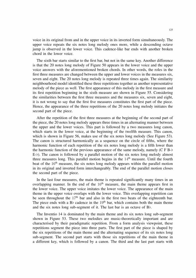
125

voice in its original from and in the upper voice in its inverted form simultaneously. Theupper voice repeats the six notes long melody ones more, while a descending octavejump is observed in the lower voice. This cadence-like bar ends with another brokenchord in the lower voice.

The sixth bar starts similar to the first bar, but not in the same key. Another differenceis that the 20 notes long melody of Figure 50 appears in the lower voice and the uppervoice answers with the aforementioned broken chords. In other words, the roles in thefirst three measures are changed between the upper and lower voices in the measures six,seven and eight. The 20 notes long melody is repeated three times again. The similarityneighbourhood model identified these three repetitions together as another representativemelody of the piece as well. The first appearance of this melody in the first measure andits first repetition beginning in the sixth measure are shown in Figure 55. Consideringthe similarities between the first three measures and the measures six, seven and eight,it is not wrong to say that the first five measures constitutes the first part of the piece.Hence, the appearance of the three repetitions of the 20 notes long melody initiates thesecond part of the piece.

After the repetition of the first three measures at the beginning of the second part ofthe piece, the 20 notes long melody appears three times in an alternating manner betweenthe upper and the lower voices. This part is followed by a two measures long canon,which starts in the lower voice, at the beginning of the twelfth measure. This canon,which is shown in Figure 56, makes use of the six notes long melody (See Figure 53).The canon is structured harmonically as a sequence on the circle of fifths, where theharmonic function of each repetition of the six notes long melody is a fifth lower thanthe harmonic function of the previous appearance of the same melody, namely (C F B-[E-[). The canon is followed by a parallel motion of the six notes long melody almostthree measures long. This parallel motion begins in the 14th measure. Until the fourthbeat of the 16th measure, the six notes long melody appears within the parallel motionin its original and inverted form interchangeably. The end of the parallel motion closesthe second part of the piece.

In the last four measures, the main theme is repeated significantly many times in anoverlapping manner. In the end of the 16th measure, the main theme appears first inthe lower voice. The upper voice imitates the lower voice. The appearance of the maintheme in the upper voice overlaps with the lower voice. This overlapping repetition canbe seen throughout the 17th bar and also in the first two beats of the eighteenth bar.The piece ends with a B[ cadence in the 19th bar, which contains both the main themeand the six notes long sub-segment of it. The last bar is an octave of B[.

The Inventio 14 is dominated by the main theme and its six notes long sub-segmentshown in Figure 53. These two melodies are music-theoretically important and arecharacterised by their paradigmatic repetition. From a form analysis viewpoint, theserepetitions segment the piece into three parts. The first part of the piece is shaped bythe six repetitions of the main theme and the alternating sequence of its six notes longsub-segment. The second part starts with those six repetitions of the main theme ina different key, which is followed by a canon. The third and the last part starts with

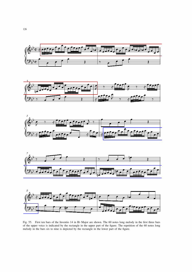
126

Fig. 55. First ten bars of the Inventio 14 in B[ Major are shown. The 60 notes long melody in the first three barsof the upper voice is indicated by the rectangle in the upper part of the figure. The repetition of the 60 notes longmelody in the bars six to nine is depicted by the rectangle in the lower part of the figure.

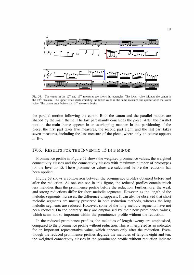
127

Fig. 56. The canon in the 12th and 13th measures are shown in rectangles. The lower voice initiates the canon inthe 12th measure. The upper voice starts imitating the lower voice in the same measure one quarter after the lowervoice. The canon ends before the 14th measure begins.

the parallel motion following the canon. Both the canon and the parallel motion areshaped by the main theme. The last part mainly concludes the piece. After the parallelmotion, the main theme appears in an overlapping manner. In this partitioning of thepiece, the first part takes five measures, the second part eight, and the last part takesseven measures, including the last measure of the piece, where only an octave appearsin B-[.

IV.6. RESULTS FOR THE INVENTIO 15 IN B MINOR

Prominence profile in Figure 57 shows the weighted prominence values, the weightedconnectivity classes and the connectivity classes with maximum number of prototypesfor the Inventio 15. These prominence values are calculated before the reduction hasbeen applied.

Figure 58 shows a comparison between the prominence profiles obtained before andafter the reduction. As one can see in this figure, the reduced profiles contain muchless melodies than the prominence profile before the reduction. Furthermore, the weakand strong reductions differ for short melodic segments. However, as the length of themelodic segments increases, the difference disappears. It can also be observed that shortmelodic segments are mostly preserved in both reduction methods, whereas the longmelodic segments are reduced. However, some of the long melodic segments have notbeen reduced. On the contrary, they are emphasised by their new prominence values,which seem not so important within the prominence profile without the reduction.

In the reduced prominence profiles, the melodies of length twenty are emphasised,compared to the prominence profile without reduction. This is interpreted as an indicatorfor an important representative value, which appears only after the reduction. Even-though the reduced prominence profiles degrade the melodies of lengths eight and ten,the weighted connectivity classes in the prominence profile without reduction indicate

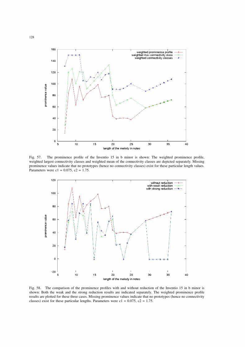
128

Fig. 57. The prominence profile of the Inventio 15 in b minor is shown: The weighted prominence profile,weighted largest connectivity classes and weighted mean of the connectivity classes are depicted separately. Missingprominence values indicate that no prototypes (hence no connectivity classes) exist for these particular length values.Parameters were c1 = 0.075, c2 = 1.75.

Fig. 58. The comparison of the prominence profiles with and without reduction of the Inventio 15 in b minor isshown: Both the weak and the strong reduction results are indicated separately. The weighted prominence profileresults are plotted for these three cases. Missing prominence values indicate that no prototypes (hence no connectivityclasses) exist for these particular lengths. Parameters were c1 = 0.075, c2 = 1.75.

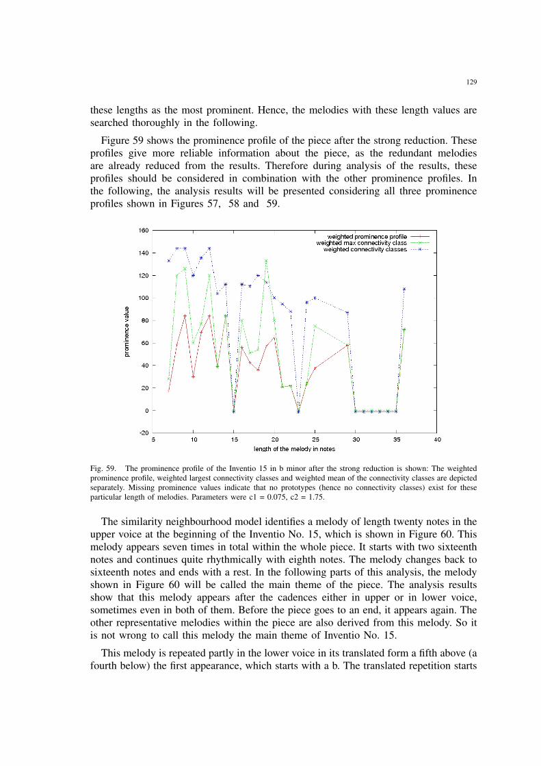
129

these lengths as the most prominent. Hence, the melodies with these length values aresearched thoroughly in the following.

Figure 59 shows the prominence profile of the piece after the strong reduction. Theseprofiles give more reliable information about the piece, as the redundant melodiesare already reduced from the results. Therefore during analysis of the results, theseprofiles should be considered in combination with the other prominence profiles. Inthe following, the analysis results will be presented considering all three prominenceprofiles shown in Figures 57, 58 and 59.

Fig. 59. The prominence profile of the Inventio 15 in b minor after the strong reduction is shown: The weightedprominence profile, weighted largest connectivity classes and weighted mean of the connectivity classes are depictedseparately. Missing prominence values indicate that no prototypes (hence no connectivity classes) exist for theseparticular length of melodies. Parameters were c1 = 0.075, c2 = 1.75.

The similarity neighbourhood model identifies a melody of length twenty notes in theupper voice at the beginning of the Inventio No. 15, which is shown in Figure 60. Thismelody appears seven times in total within the whole piece. It starts with two sixteenthnotes and continues quite rhythmically with eighth notes. The melody changes back tosixteenth notes and ends with a rest. In the following parts of this analysis, the melodyshown in Figure 60 will be called the main theme of the piece. The analysis resultsshow that this melody appears after the cadences either in upper or in lower voice,sometimes even in both of them. Before the piece goes to an end, it appears again. Theother representative melodies within the piece are also derived from this melody. So itis not wrong to call this melody the main theme of Inventio No. 15.

This melody is repeated partly in the lower voice in its translated form a fifth above (afourth below) the first appearance, which starts with a b. The translated repetition starts

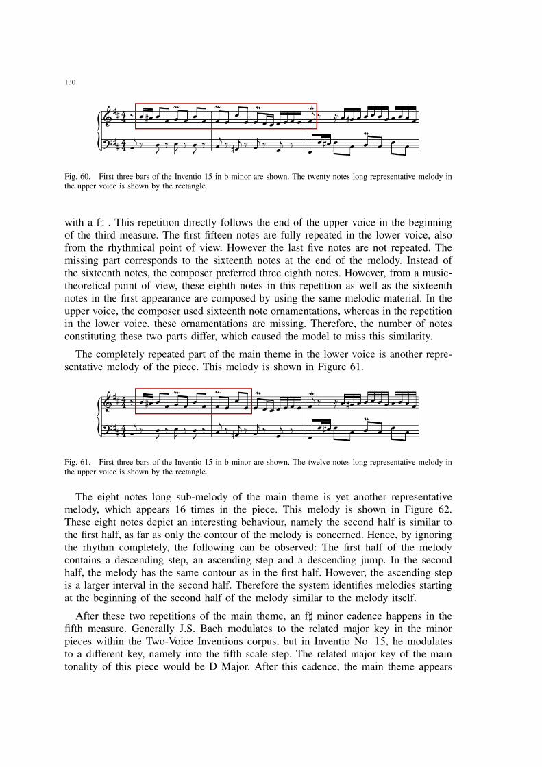
130

Fig. 60. First three bars of the Inventio 15 in b minor are shown. The twenty notes long representative melody inthe upper voice is shown by the rectangle.

with a f] . This repetition directly follows the end of the upper voice in the beginningof the third measure. The first fifteen notes are fully repeated in the lower voice, alsofrom the rhythmical point of view. However the last five notes are not repeated. Themissing part corresponds to the sixteenth notes at the end of the melody. Instead ofthe sixteenth notes, the composer preferred three eighth notes. However, from a music-theoretical point of view, these eighth notes in this repetition as well as the sixteenthnotes in the first appearance are composed by using the same melodic material. In theupper voice, the composer used sixteenth note ornamentations, whereas in the repetitionin the lower voice, these ornamentations are missing. Therefore, the number of notesconstituting these two parts differ, which caused the model to miss this similarity.

The completely repeated part of the main theme in the lower voice is another repre-sentative melody of the piece. This melody is shown in Figure 61.

Fig. 61. First three bars of the Inventio 15 in b minor are shown. The twelve notes long representative melody inthe upper voice is shown by the rectangle.

The eight notes long sub-melody of the main theme is yet another representativemelody, which appears 16 times in the piece. This melody is shown in Figure 62.These eight notes depict an interesting behaviour, namely the second half is similar tothe first half, as far as only the contour of the melody is concerned. Hence, by ignoringthe rhythm completely, the following can be observed: The first half of the melodycontains a descending step, an ascending step and a descending jump. In the secondhalf, the melody has the same contour as in the first half. However, the ascending stepis a larger interval in the second half. Therefore the system identifies melodies startingat the beginning of the second half of the melody similar to the melody itself.

After these two repetitions of the main theme, an f] minor cadence happens in thefifth measure. Generally J.S. Bach modulates to the related major key in the minorpieces within the Two-Voice Inventions corpus, but in Inventio No. 15, he modulatesto a different key, namely into the fifth scale step. The related major key of the maintonality of this piece would be D Major. After this cadence, the main theme appears

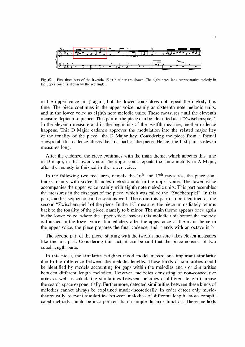
131

Fig. 62. First three bars of the Inventio 15 in b minor are shown. The eight notes long representative melody inthe upper voice is shown by the rectangle.

in the upper voice in f] again, but the lower voice does not repeat the melody thistime. The piece continues in the upper voice mainly as sixteenth note melodic units,and in the lower voice as eighth note melodic units. These measures until the eleventhmeasure depict a sequence. This part of the piece can be identified as a “Zwischenspiel”.In the eleventh measure and in the beginning of the twelfth measure, another cadencehappens. This D Major cadence approves the modulation into the related major keyof the tonality of the piece –the D Major key. Considering the piece from a formalviewpoint, this cadence closes the first part of the piece. Hence, the first part is elevenmeasures long.

After the cadence, the piece continues with the main theme, which appears this timein D major, in the lower voice. The upper voice repeats the same melody in A Major,after the melody is finished in the lower voice.

In the following two measures, namely the 16th and 17th measures, the piece con-tinues mainly with sixteenth notes melodic units in the upper voice. The lower voiceaccompanies the upper voice mainly with eighth note melodic units. This part resemblesthe measures in the first part of the piece, which was called the “Zwichenspiel”. In thispart, another sequence can be seen as well. Therefore this part can be identified as thesecond “Zwischenspiel” of the piece. In the 18th measure, the piece immediately returnsback to the tonality of the piece, namely to b minor. The main theme appears once againin the lower voice, where the upper voice answers this melodic unit before the melodyis finished in the lower voice. Immediately after the appearance of the main theme inthe upper voice, the piece prepares the final cadence, and it ends with an octave in b.

The second part of the piece, starting with the twelfth measure takes eleven measureslike the first part. Considering this fact, it can be said that the piece consists of twoequal length parts.

In this piece, the similarity neighbourhood model missed one important similaritydue to the difference between the melodic lengths. These kinds of similarities couldbe identified by models accounting for gaps within the melodies and / or similaritiesbetween different length melodies. However, melodies consisting of non-consecutivenotes as well as calculating similarities between melodies of different length increasethe search space exponentially. Furthermore, detected similarities between these kinds ofmelodies cannot always be explained music-theoretically. In order detect only music-theoretically relevant similarities between melodies of different length, more compli-cated methods should be incorporated than a simple distance function. These methods

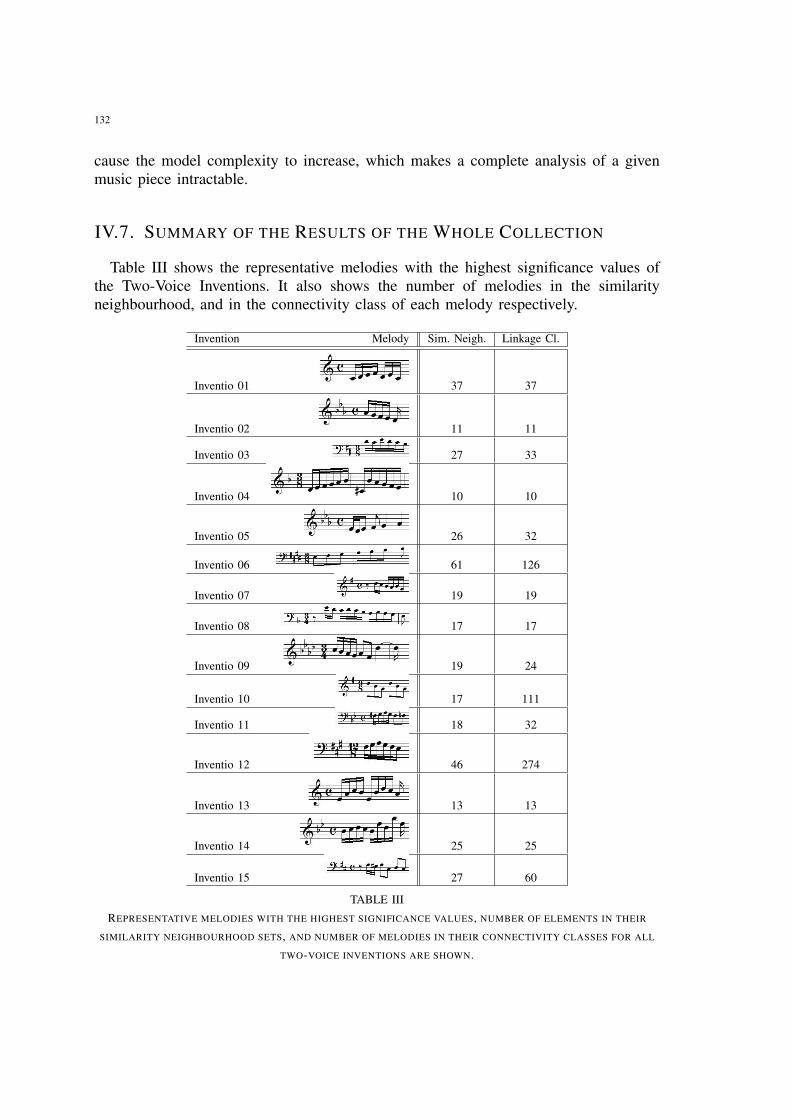
132

cause the model complexity to increase, which makes a complete analysis of a givenmusic piece intractable.

IV.7. SUMMARY OF THE RESULTS OF THE WHOLE COLLECTION

Table III shows the representative melodies with the highest significance values ofthe Two-Voice Inventions. It also shows the number of melodies in the similarityneighbourhood, and in the connectivity class of each melody respectively.

Invention Melody Sim. Neigh. Linkage Cl.

Inventio 01 37 37

Inventio 02 11 11

Inventio 03 27 33

Inventio 04 10 10

Inventio 05 26 32

Inventio 06 61 126

Inventio 07 19 19

Inventio 08 17 17

Inventio 09 19 24

Inventio 10 17 111

Inventio 11 18 32

Inventio 12 46 274

Inventio 13 13 13

Inventio 14 25 25

Inventio 15 27 60

TABLE III

REPRESENTATIVE MELODIES WITH THE HIGHEST SIGNIFICANCE VALUES, NUMBER OF ELEMENTS IN THEIR

SIMILARITY NEIGHBOURHOOD SETS, AND NUMBER OF MELODIES IN THEIR CONNECTIVITY CLASSES FOR ALL

TWO-VOICE INVENTIONS ARE SHOWN.

133

The representative melodies with highest significance values correspond very well tothe traditional music-theoretical analyses [64]; if a particular main theme exists, suchas Inventio 01, 04, 09, 14.

The Inventio 02 (See Section IV.2) is a canon. As I indicated in the correspondingsection, this piece repeats a melody in a time-delayed fashion, and does not possess ashort melodic segment, which can be identified as the main theme of the piece, as inthe Inventio 01. However, as I showed in the corresponding section as well, the canoncan be tracked by the model very well by just following the representative melodiesappearing consecutively.

In the Inventio 06, an exchange between the voices happens in the beginning of thefifth measure. The first four measures in the upper voice are repeated in the lower voicebetween the fifth and eighth measures, where in the same four measures, the uppervoice repeats the first four measures of the lower voice.

The first four measures of the Inventio 07 repeat the melody shown in Table III eighttimes in total in alternating manner.

For the Inventio 10, Inventio 12 and Inventio 15, the unification process leads to largeconnectivity classes. This behaviour is a very good example of higher order similarities.The melodic segments, which connect the similarity neighbourhoods are interesting toobserve (See Section IV.6).

Especially the Inventio 10 is not a highly melodic piece. The piece is composedmainly by using broken chords in both upper and lower voices. Therefore the similarityneighbourhood model detected mainly phrases consisting of series of these brokenchords.

The Inventio 08 depicts a similar behaviour to the Inventio 10. However, the piececonsists also of canon parts. Especially in the first three measures, similar to the casein the Inventio 06, the melodic progression moves between the two voices of the piecealternatingly. This behaviour appears several times within the piece. Different from theInventio 06, in the Inventio 08, the first measure of the upper voice is repeated in thesecond measure of the lower voice and in the third measure of the upper voice again.Hence the same melody moves from the upper voice to the lower voice and back to theupper voice again. At the same time, the second measure of the upper voice appears inthe third measure the lower voice. If these changes between the voices are consideredto be sub-segments of the same melody, the similarity neighbourhood model can notdetect these kinds of changes between the voices of the piece directly, since a melodyis defined to be within a particular voice. Nonetheless, these exchanges can still beconstructed after observing, where the representative melodies appear.

The results of the Inventions 01, 02, 04, 09, 14 and 15, and even these extremelysummarised results, show that the corpus 15 Two-Voice Inventions is in-homogeneous,with respect to melodic connectivity. Different compositional techniques dominate dif-ferent Inventions. Therefore, the analysis procedure of each Invention is a small researchproject on its own. However, the similarity neighbourhood model can depict differentaspects of these small pieces in a proper way.

134

135

V. ANALYSIS OF TWO-VOICEINVENTIONS WITH THE GENETIC

ALGORITHMS

V.1. APPROXIMATION RESULTS OF THE TWO-VOICE INVENTIONS

In order to test the performance of the accelerated approximation of the similar-ity neighbourhood model with genetic algorithms, the Two-Voice Inventions of J. S.BACH [12] have been analysed again.

In these experiments, the following values have been chosen for the constants:

POPULATION_RATE = 0.1CROSSOVER_RATE = 0.25MUTATION_RATE = 0.1MINIMUM_LENGTH = 4

The results of these experiments are presented not only in musical notation, butalso in two other formats. The first format is called Humdrum [37] [38]. Humdrumis a general-purpose software system developed to assist music researchers (See theAppendix). The second format is a list conforming to the LISP programming language.The object oriented extension CLOS of the LISP programming language is used by thesoftware Open Music [39]. Open Music is developed by IRCAM Paris, which is aninstitute supporting contemporary music research and production.

The analysis results of the similarity neighbourhood model has already been presentedin Chapter IV. Therefore they will not be repeated in this chapter. Instead of that,the difference between the durations needed for the method with and without thegenetic algorithms to analyse a piece are given here. Table IV shows these durations ina comparison. Obviously the method approximated with genetic algorithms is muchfaster than the original method. The biggest difference between genetic algorithmsapproximation and the original method occurs for the Inventio 07, namely geneticalgorithms are 17.70 times faster than the original method. The lowest difference occursfor the Inventio 10, namely 3.77 times. This time difference does not give any clue abouthow close the approximation to the original analysis is. The approximated analysisresults are a sub-set of the original analysis results of a given piece. The experimentshave shown that this sub-set generally contains the most important part of the originalanalysis. However, because of the stochastic nature of genetic algorithms, in eachexperimentation, the results obtained by the genetic algorithms slightly differ from theothers. Furthermore, the time it takes to perform the analysis differs as well. Nevertheless

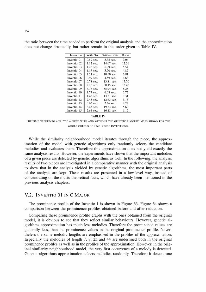
136

the ratio between the time needed to perform the original analysis and the approximationdoes not change drastically, but rather remain in this order given in Table IV.

Invention With GA Without GA RatioInventio 01 0.59 sec. 5.35 sec. 9.06Inventio 02 1.12 sec. 14.07 sec. 12.56Inventio 03 1.26 sec. 6.99 sec. 5.54Inventio 04 1.17 sec. 5.70 sec. 4.87Inventio 05 1.54 sec. 10.50 sec. 6.81Inventio 06 0.99 sec. 4.59 sec. 4.63Inventio 07 0.78 sec. 13.81 sec. 17.70Inventio 08 2.25 sec. 30.15 sec. 13.40Inventio 09 6.78 sec. 55.94 sec. 8.25Inventio 10 1.77 sec. 6.68 sec. 3.77Inventio 11 1.45 sec. 13.51 sec. 9.31Inventio 12 2.45 sec. 12.63 sec. 5.15Inventio 13 0.65 sec. 2.76 sec. 4.24Inventio 14 3.45 sec. 19.33 sec. 5.60Inventio 15 2.64 sec. 16.18 sec. 6.12

TABLE IV

THE TIME NEEDED TO ANALYSE A PIECE WITH AND WITHOUT THE GENETIC ALGORITHMS IS SHOWN FOR THE

WHOLE CORPUS OF TWO-VOICE INVENTIONS.

While the similarity neighbourhood model iterates through the piece, the approx-imation of the model with genetic algorithms only randomly selects the candidatemelodies and evaluates them. Therefore this approximation does not yield exactly thesame analysis results. However, the experiments have shown that the important melodiesof a given piece are detected by genetic algorithms as well. In the following, the analysisresults of two pieces are investigated in a comparative manner with the original analysisto show that in the analysis yielded by genetic algorithms, the most important partsof the analysis are kept. These results are presented in a low-level way, instead ofconcentrating on the music theoretical facts, which have already been mentioned in theprevious analysis chapters.

V.2. INVENTIO 01 IN C MAJOR

The prominence profile of the Inventio 1 is shown in Figure 63. Figure 64 shows acomparison between the prominence profiles obtained before and after reduction.

Comparing these prominence profile graphs with the ones obtained from the originalmodel, it is obvious to see that they reflect similar behaviours. However, genetic al-gorithms approximation has much less melodies. Therefore the prominence values aregenerally less, than the prominence values in the original prominence profile. Never-theless the same melodic lengths are emphasised in the profiles of the approximation.Especially the melodies of length 7, 8, 25 and 44 are underlined both in the originalprominence profiles as well as in the profiles of the approximation. However, in the orig-inal similarity neighbourhood model, the very first occurrence of a melody is detected.Genetic algorithms approximation selects melodies randomly. Therefore it detects one

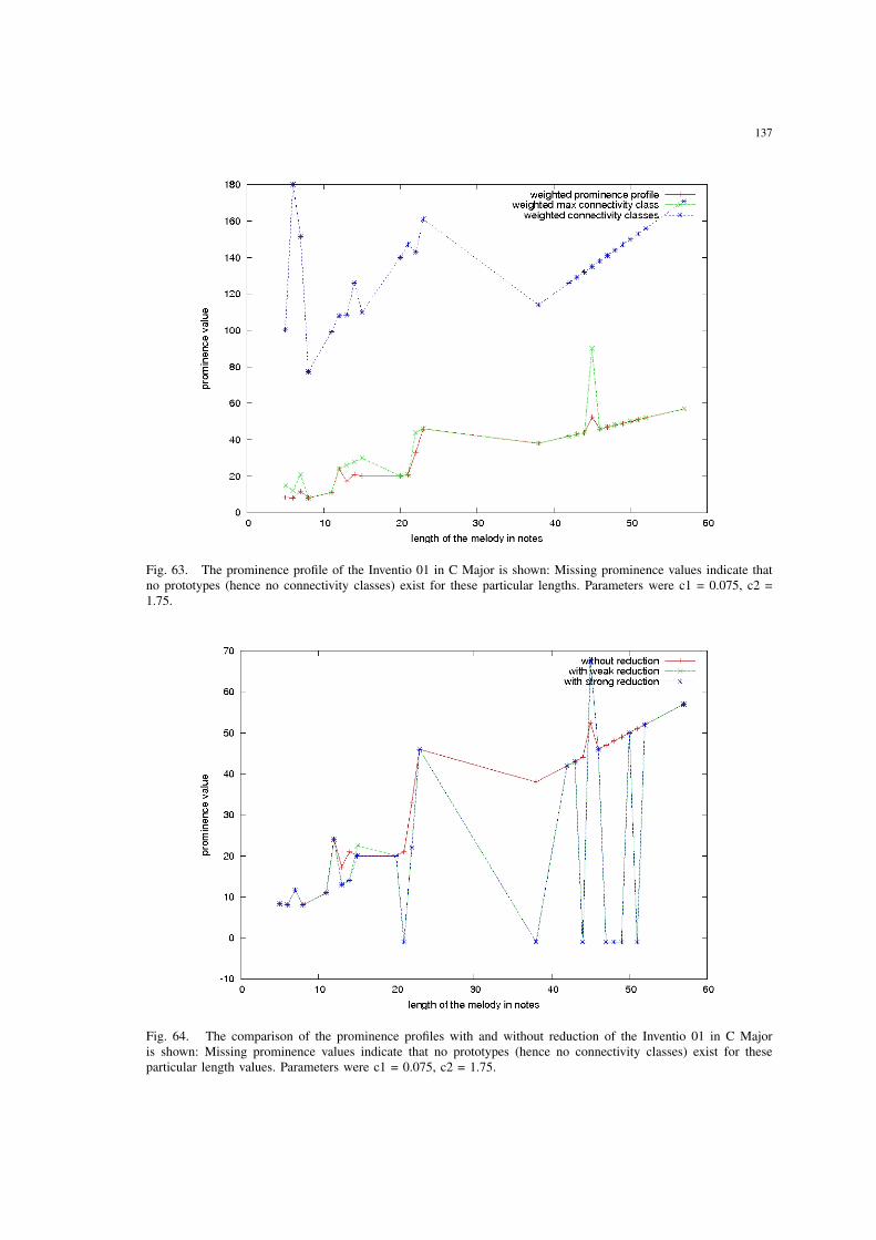
137

Fig. 63. The prominence profile of the Inventio 01 in C Major is shown: Missing prominence values indicate thatno prototypes (hence no connectivity classes) exist for these particular lengths. Parameters were c1 = 0.075, c2 =1.75.

Fig. 64. The comparison of the prominence profiles with and without reduction of the Inventio 01 in C Majoris shown: Missing prominence values indicate that no prototypes (hence no connectivity classes) exist for theseparticular length values. Parameters were c1 = 0.075, c2 = 1.75.

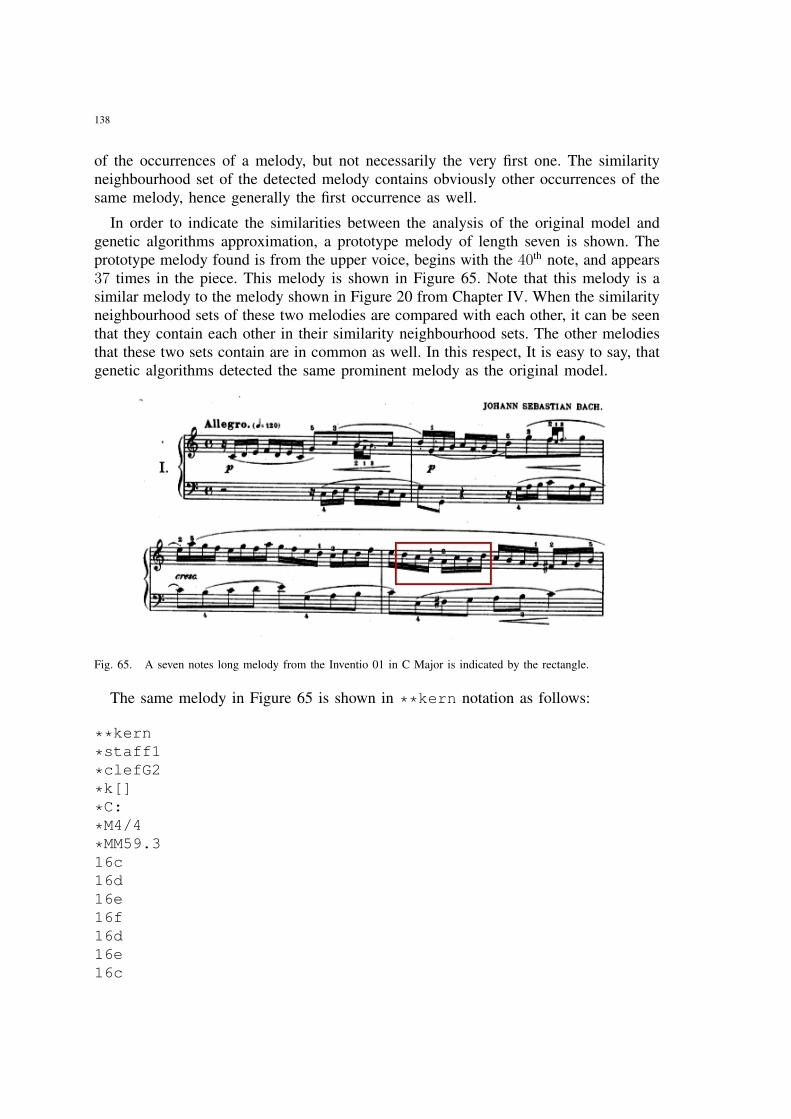
138

of the occurrences of a melody, but not necessarily the very first one. The similarityneighbourhood set of the detected melody contains obviously other occurrences of thesame melody, hence generally the first occurrence as well.

In order to indicate the similarities between the analysis of the original model andgenetic algorithms approximation, a prototype melody of length seven is shown. Theprototype melody found is from the upper voice, begins with the 40th note, and appears37 times in the piece. This melody is shown in Figure 65. Note that this melody is asimilar melody to the melody shown in Figure 20 from Chapter IV. When the similarityneighbourhood sets of these two melodies are compared with each other, it can be seenthat they contain each other in their similarity neighbourhood sets. The other melodiesthat these two sets contain are in common as well. In this respect, It is easy to say, thatgenetic algorithms detected the same prominent melody as the original model.

Fig. 65. A seven notes long melody from the Inventio 01 in C Major is indicated by the rectangle.

The same melody in Figure 65 is shown in **kern notation as follows:

**kern

*staff1

*clefG2

*k[]

*C:

*M4/4

*MM59.316c16d16e16f16d16e16c

139

*-

The **kern notation is the standard representation format of Humdrum system. The**kern notation is a tabular notation system. In this notation, each part is representedas a column. Each column has the typical properties of a musical part, like the clef,the signature of the accidentals, the tempo and metrum, etc. In this example, the actualmelody starts in the eighth line, namely with the line 16c which indicates that thecorresponding note is a sixteenth middle c.

This melody is quite dominant in the whole piece, as indicated in Section IV.1. Adetailed analysis of the piece can be found in the corresponding section.

The following notation represents the similarity neighbourhood set of the same mel-ody in LISP format, which is suitable for the Open Music program. Each line corre-sponds to one voice of the given piece. The numbers in parentheses are the note numbers,where the melody appears within the particular voice. The very first occurrences of themelody in both voices of the piece are at the very beginning of the piece, namelystarting with the zeroth note until the sixth note.

(((0 1 2 3 4 5 6 )(9 10 11 12 13 14 15 )(31 32 33 34 35 36 37)...)((0 1 2 3 4 5 6 )(12 13 14 15 16 17 18)(24 25 26 27 28 29 30 )...))

The examples from the approximated analysis can be extended to show more commonmelodies from both analyses. The prototype melodies detected by genetic algorithms arethe ones from the original analysis with high significance values. In order to demonstratethis behaviour further, the analysis results of the Invenio 04 are shown in the followingsection.

V.3. INVENTIO 04 IN D MINOR

The approximated prominence profile of the Inventio 4 is shown in Figure 66.Figure 67 shows a comparison between the prominence profiles obtained before andafter reduction.

These prominence profiles shown in Figures 66 and 67 point out the same lengthvalues as the original model. Especially the length of twelve notes is emphasised inthese prominence profiles. The comparison of the reduced profiles with the unreducedone indicates that not so many melodies have been reduced from the results. This is aneffect of genetic algorithms that genetic algorithms extract the most prominent melodiesin a given piece.

A single sample melody cannot prove that the analysis results converge to the realanalysis of a given piece. However repeating a whole analysis does not make muchmore sense either. Therefore, I present sample prototype melody, detected by geneticalgorithms, which has also been identified by the original analysis and by the musictheory as a prominent melody of the piece. The sample melody that I present here is

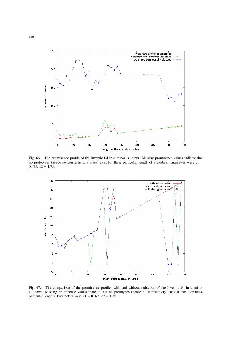
140

Fig. 66. The prominence profile of the Inventio 04 in d minor is shown: Missing prominence values indicate thatno prototypes (hence no connectivity classes) exist for these particular length of melodies. Parameters were c1 =0.075, c2 = 1.75.

Fig. 67. The comparison of the prominence profiles with and without reduction of the Inventio 04 in d minoris shown: Missing prominence values indicate that no prototypes (hence no connectivity classes) exist for theseparticular lengths. Parameters were c1 = 0.075, c2 = 1.75.

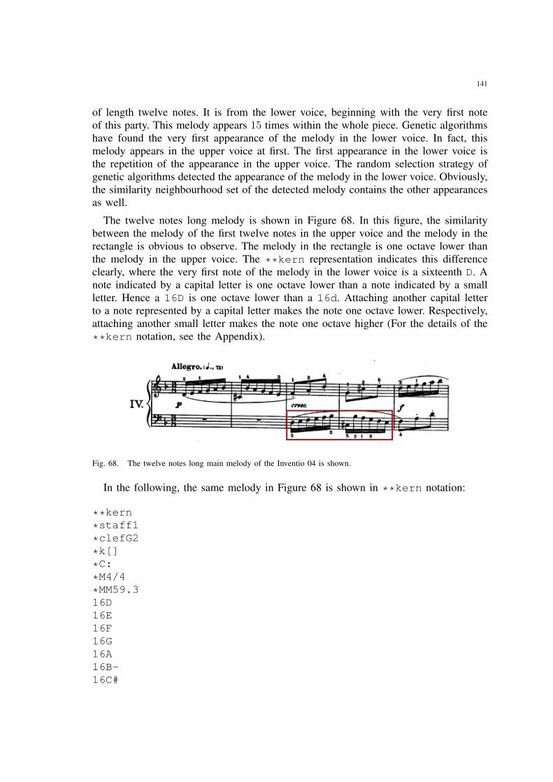
141

of length twelve notes. It is from the lower voice, beginning with the very first noteof this party. This melody appears 15 times within the whole piece. Genetic algorithmshave found the very first appearance of the melody in the lower voice. In fact, thismelody appears in the upper voice at first. The first appearance in the lower voice isthe repetition of the appearance in the upper voice. The random selection strategy ofgenetic algorithms detected the appearance of the melody in the lower voice. Obviously,the similarity neighbourhood set of the detected melody contains the other appearancesas well.

The twelve notes long melody is shown in Figure 68. In this figure, the similaritybetween the melody of the first twelve notes in the upper voice and the melody in therectangle is obvious to observe. The melody in the rectangle is one octave lower thanthe melody in the upper voice. The **kern representation indicates this differenceclearly, where the very first note of the melody in the lower voice is a sixteenth D. Anote indicated by a capital letter is one octave lower than a note indicated by a smallletter. Hence a 16D is one octave lower than a 16d. Attaching another capital letterto a note represented by a capital letter makes the note one octave lower. Respectively,attaching another small letter makes the note one octave higher (For the details of the**kern notation, see the Appendix).

Fig. 68. The twelve notes long main melody of the Inventio 04 is shown.

In the following, the same melody in Figure 68 is shown in **kern notation:

**kern

*staff1

*clefG2

*k[]

*C:

*M4/4

*MM59.316D16E16F16G16A16B-16C#

142

16B-16A16G16F16E

*-

As mentioned in the analysis of the Inventio 04 in Section IV.3, this melody is one ofthe most important ones within the piece. The approximation with genetic algorithmsdetects this melody as well.

In general, genetic algorithms extract an important sub-set of the whole analysisresults of the similarity neighbourhood model. Even-though it is only an approximationof the original model, most of the significant information from the result of the originalmodel are contained within the approximated results as well. Therefore, especially forrelatively long orchestral pieces, which generally consist of even more than four orfive voices, genetic algorithms approximation can be incorporated reliably. The yieldedresults provide a satisfactory approximation of the original model.

143

VI. ANALYSIS OF KEREN

The similarity neighbourhood model was also tested on a solo trombone piece calledKeren of Iannis Xenakis, which was composed in 1986. Although the similarity neigh-bourhood model does not include stylistic presuppositions, the application to tonal pieceswas motivated by the typically high amount of paradigmatic repetition depending onthe contours of melodic segments. Keren does not contain similar melodic segmentsin the sense of motivic paradigms in the baroque or classical period of western music.While this approach has been successfully applied to pieces of the tonal period, it wasa particular challenge to test it for a non-tonal piece like Keren. With this respect,the analysis of Keren had to take a slightly different route than analysing 15 two-partinventions of J.S.Bach.

The results of these experiments are going to be presented in this chapter [10].Experimental results are presented again in a music-theoretical context, in order toeasily observe the music-theoretical relevance of the results. The computational resultswere thoroughly discussed with experts of music theory. The experts confirmed that theobtained connectivity classes represent music-theoretically relevant paradigms.

VI.1. THE PROMINENCE PROFILE OF KEREN

The prominence profile in Figure 69 shows the prominence values for each length ofprototypes, the weighted connectivity classes and the connectivity classes with maximumnumber of prototypes for Keren.

The longest prototype, which can be identified by the model is 49 notes long. As itcan easily be seen on the profile, the prominence values of the longer melodic segmentsare remarkably less than the prominence values of the short melodic segments, whichwas not the case in Two-Voice Inventions. This fact indicates that Keren is not a melodicpiece in the sense that melodies are repeated and subdivided into sub melodies, whichare also repeated within the piece a lot of times. Instead of this melodic decomposition,Keren shows that the generally shorter segments play a more important role in the piece,and especially where these melodic segments appear, and where they do not appear isimportant to understand the structure of the piece.

Figure 70 shows a comparison between the prominence profiles obtained before andafter the reduction. In general, reduction process eliminates a noticeable amount ofprototypes identified by the model. The remaining prototypes are the melodic segments,for which it is more likely that they play an important role within the piece. As one cansee in this figure, the reduced profiles contain only a little less number of prototypes thanbefore reduction. This is another indicator about Keren being not a melodic piece in theclassical sense. Furthermore, there are several lengths, for which the prominence valuedoes not decrease after the reduction. These melodic segments deserve more attention.

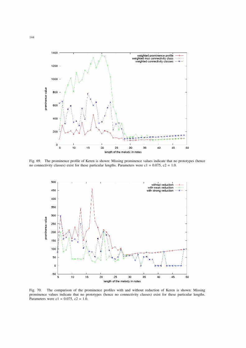
144

Fig. 69. The prominence profile of Keren is shown: Missing prominence values indicate that no prototypes (henceno connectivity classes) exist for these particular lengths. Parameters were c1 = 0.075, c2 = 1.0.

Fig. 70. The comparison of the prominence profiles with and without reduction of Keren is shown: Missingprominence values indicate that no prototypes (hence no connectivity classes) exist for these particular lengths.Parameters were c1 = 0.075, c2 = 1.0.

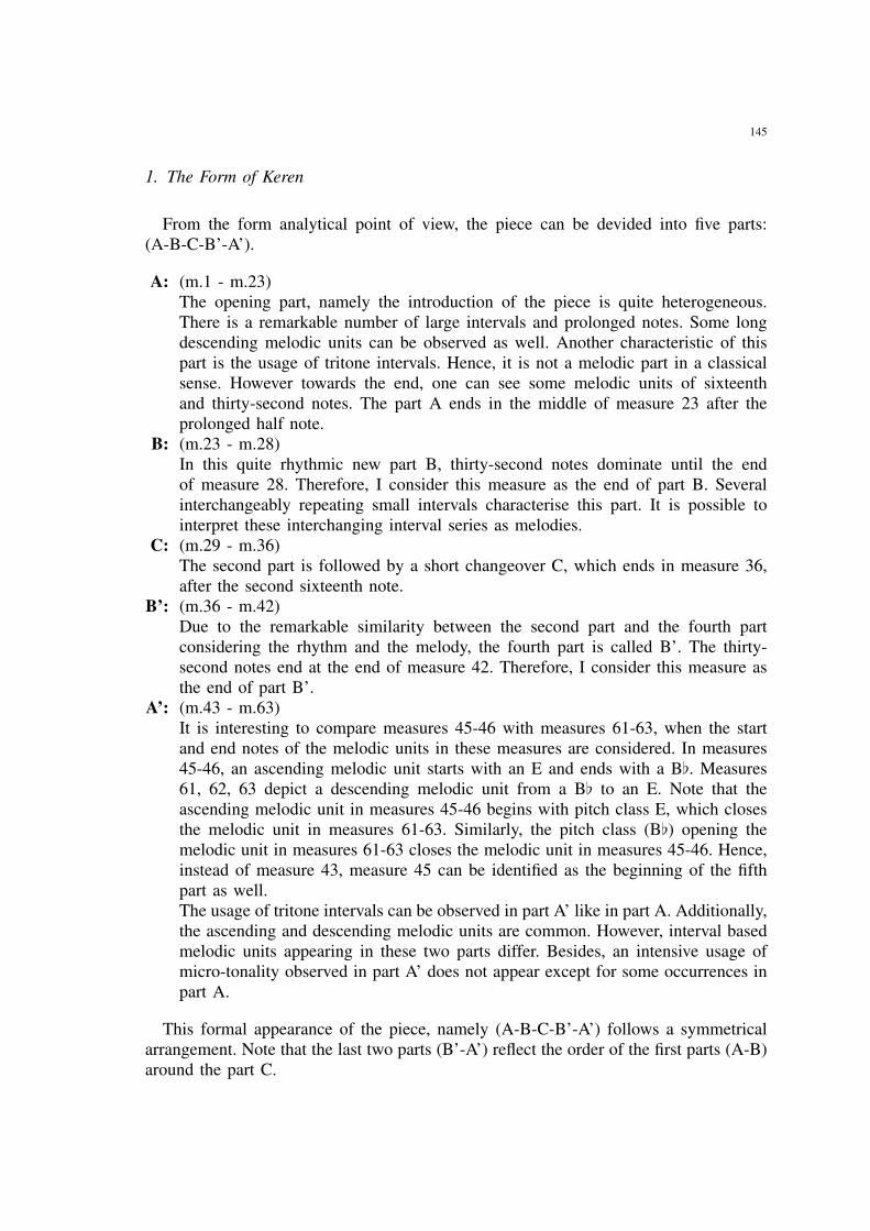
145

1. The Form of Keren

From the form analytical point of view, the piece can be devided into five parts:(A-B-C-B’-A’).

A: (m.1 - m.23)The opening part, namely the introduction of the piece is quite heterogeneous.There is a remarkable number of large intervals and prolonged notes. Some longdescending melodic units can be observed as well. Another characteristic of thispart is the usage of tritone intervals. Hence, it is not a melodic part in a classicalsense. However towards the end, one can see some melodic units of sixteenthand thirty-second notes. The part A ends in the middle of measure 23 after theprolonged half note.

B: (m.23 - m.28)In this quite rhythmic new part B, thirty-second notes dominate until the endof measure 28. Therefore, I consider this measure as the end of part B. Severalinterchangeably repeating small intervals characterise this part. It is possible tointerpret these interchanging interval series as melodies.

C: (m.29 - m.36)The second part is followed by a short changeover C, which ends in measure 36,after the second sixteenth note.

B’: (m.36 - m.42)Due to the remarkable similarity between the second part and the fourth partconsidering the rhythm and the melody, the fourth part is called B’. The thirty-second notes end at the end of measure 42. Therefore, I consider this measure asthe end of part B’.

A’: (m.43 - m.63)It is interesting to compare measures 45-46 with measures 61-63, when the startand end notes of the melodic units in these measures are considered. In measures45-46, an ascending melodic unit starts with an E and ends with a B[. Measures61, 62, 63 depict a descending melodic unit from a B[ to an E. Note that theascending melodic unit in measures 45-46 begins with pitch class E, which closesthe melodic unit in measures 61-63. Similarly, the pitch class (B[) opening themelodic unit in measures 61-63 closes the melodic unit in measures 45-46. Hence,instead of measure 43, measure 45 can be identified as the beginning of the fifthpart as well.The usage of tritone intervals can be observed in part A’ like in part A. Additionally,the ascending and descending melodic units are common. However, interval basedmelodic units appearing in these two parts differ. Besides, an intensive usage ofmicro-tonality observed in part A’ does not appear except for some occurrences inpart A.

This formal appearance of the piece, namely (A-B-C-B’-A’) follows a symmetricalarrangement. Note that the last two parts (B’-A’) reflect the order of the first parts (A-B)around the part C.

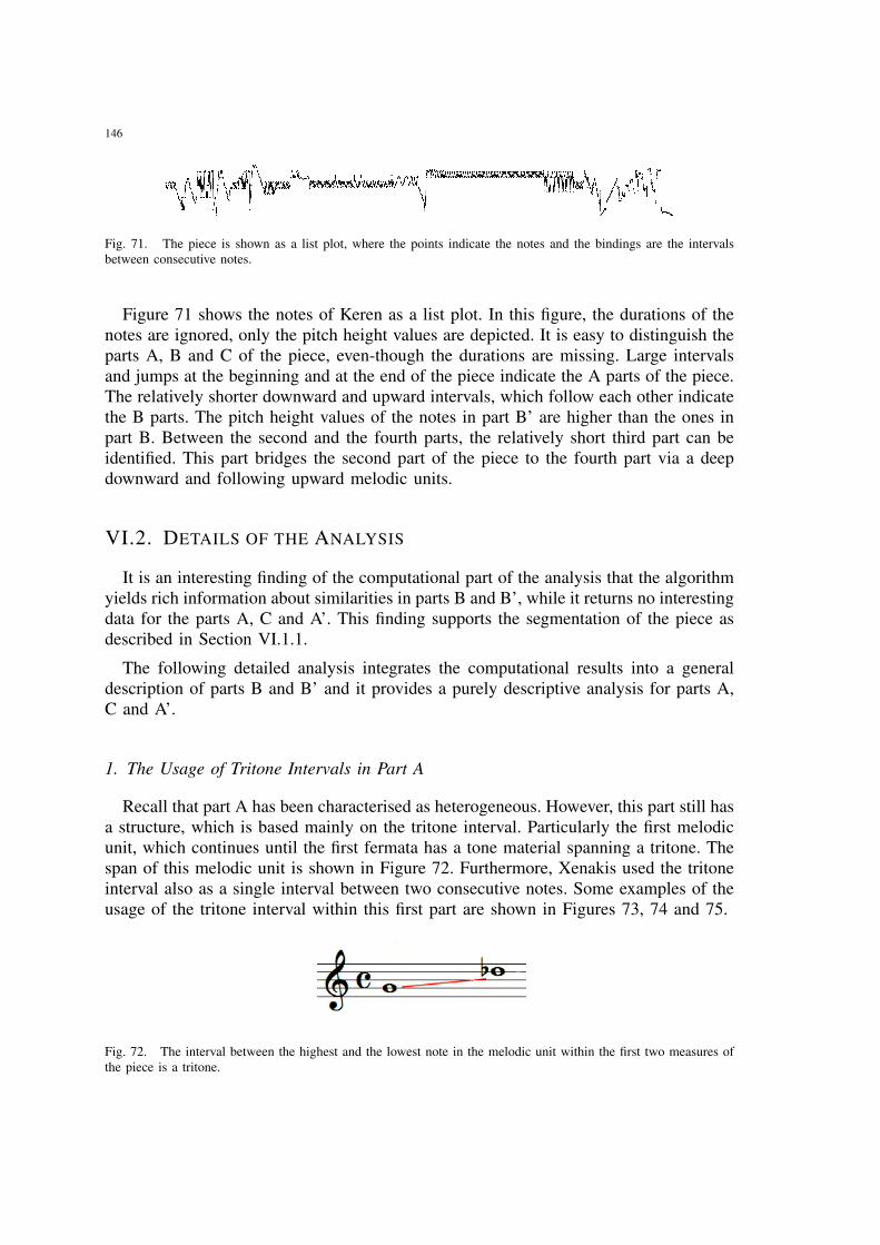
146

Fig. 71. The piece is shown as a list plot, where the points indicate the notes and the bindings are the intervalsbetween consecutive notes.

Figure 71 shows the notes of Keren as a list plot. In this figure, the durations of thenotes are ignored, only the pitch height values are depicted. It is easy to distinguish theparts A, B and C of the piece, even-though the durations are missing. Large intervalsand jumps at the beginning and at the end of the piece indicate the A parts of the piece.The relatively shorter downward and upward intervals, which follow each other indicatethe B parts. The pitch height values of the notes in part B’ are higher than the ones inpart B. Between the second and the fourth parts, the relatively short third part can beidentified. This part bridges the second part of the piece to the fourth part via a deepdownward and following upward melodic units.

VI.2. DETAILS OF THE ANALYSIS

It is an interesting finding of the computational part of the analysis that the algorithmyields rich information about similarities in parts B and B’, while it returns no interestingdata for the parts A, C and A’. This finding supports the segmentation of the piece asdescribed in Section VI.1.1.

The following detailed analysis integrates the computational results into a generaldescription of parts B and B’ and it provides a purely descriptive analysis for parts A,C and A’.

1. The Usage of Tritone Intervals in Part A

Recall that part A has been characterised as heterogeneous. However, this part still hasa structure, which is based mainly on the tritone interval. Particularly the first melodicunit, which continues until the first fermata has a tone material spanning a tritone. Thespan of this melodic unit is shown in Figure 72. Furthermore, Xenakis used the tritoneinterval also as a single interval between two consecutive notes. Some examples of theusage of the tritone interval within this first part are shown in Figures 73, 74 and 75.

Fig. 72. The interval between the highest and the lowest note in the melodic unit within the first two measures ofthe piece is a tritone.

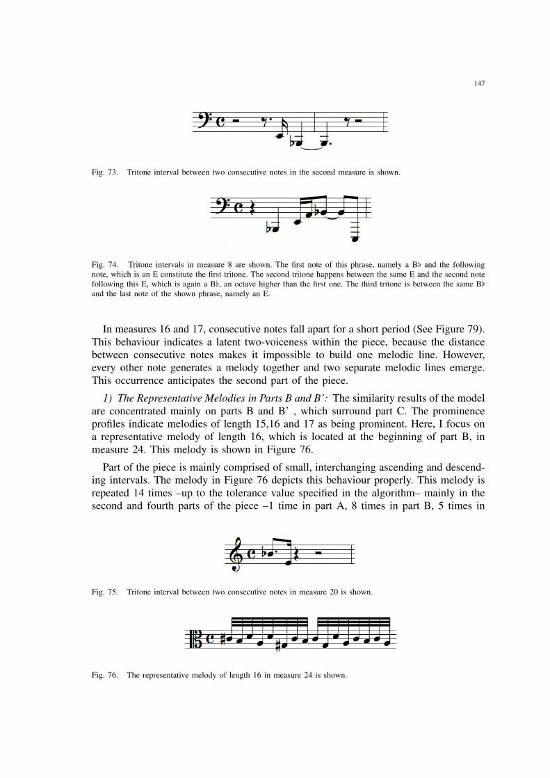
147

Fig. 73. Tritone interval between two consecutive notes in the second measure is shown.

Fig. 74. Tritone intervals in measure 8 are shown. The first note of this phrase, namely a B[ and the followingnote, which is an E constitute the first tritone. The second tritone happens between the same E and the second notefollowing this E, which is again a B[, an octave higher than the first one. The third tritone is between the same B[and the last note of the shown phrase, namely an E.

In measures 16 and 17, consecutive notes fall apart for a short period (See Figure 79).This behaviour indicates a latent two-voiceness within the piece, because the distancebetween consecutive notes makes it impossible to build one melodic line. However,every other note generates a melody together and two separate melodic lines emerge.This occurrence anticipates the second part of the piece.

1) The Representative Melodies in Parts B and B’: The similarity results of the modelare concentrated mainly on parts B and B’ , which surround part C. The prominenceprofiles indicate melodies of length 15,16 and 17 as being prominent. Here, I focus ona representative melody of length 16, which is located at the beginning of part B, inmeasure 24. This melody is shown in Figure 76.

Part of the piece is mainly comprised of small, interchanging ascending and descend-ing intervals. The melody in Figure 76 depicts this behaviour properly. This melody isrepeated 14 times –up to the tolerance value specified in the algorithm– mainly in thesecond and fourth parts of the piece –1 time in part A, 8 times in part B, 5 times in

Fig. 75. Tritone interval between two consecutive notes in measure 20 is shown.

Fig. 76. The representative melody of length 16 in measure 24 is shown.

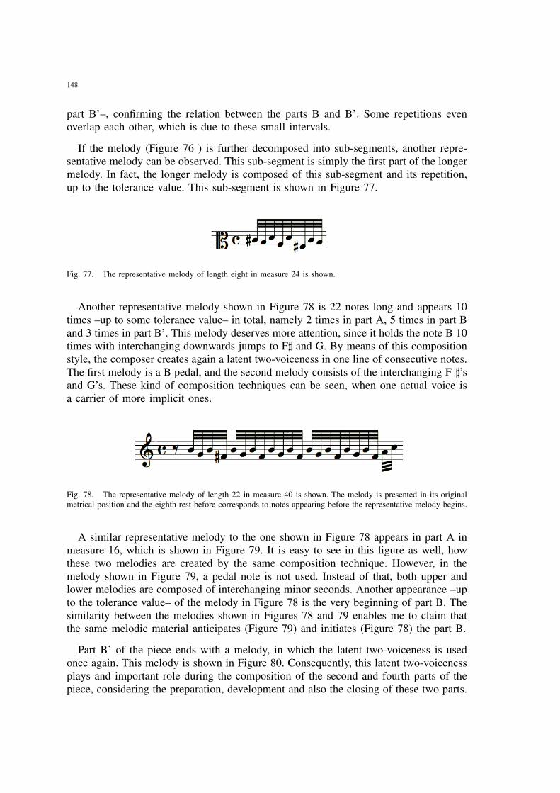
148

part B’–, confirming the relation between the parts B and B’. Some repetitions evenoverlap each other, which is due to these small intervals.

If the melody (Figure 76 ) is further decomposed into sub-segments, another repre-sentative melody can be observed. This sub-segment is simply the first part of the longermelody. In fact, the longer melody is composed of this sub-segment and its repetition,up to the tolerance value. This sub-segment is shown in Figure 77.

Fig. 77. The representative melody of length eight in measure 24 is shown.

Another representative melody shown in Figure 78 is 22 notes long and appears 10times –up to some tolerance value– in total, namely 2 times in part A, 5 times in part Band 3 times in part B’. This melody deserves more attention, since it holds the note B 10times with interchanging downwards jumps to F] and G. By means of this compositionstyle, the composer creates again a latent two-voiceness in one line of consecutive notes.The first melody is a B pedal, and the second melody consists of the interchanging F-]’sand G’s. These kind of composition techniques can be seen, when one actual voice isa carrier of more implicit ones.

Fig. 78. The representative melody of length 22 in measure 40 is shown. The melody is presented in its originalmetrical position and the eighth rest before corresponds to notes appearing before the representative melody begins.

A similar representative melody to the one shown in Figure 78 appears in part A inmeasure 16, which is shown in Figure 79. It is easy to see in this figure as well, howthese two melodies are created by the same composition technique. However, in themelody shown in Figure 79, a pedal note is not used. Instead of that, both upper andlower melodies are composed of interchanging minor seconds. Another appearance –upto the tolerance value– of the melody in Figure 78 is the very beginning of part B. Thesimilarity between the melodies shown in Figures 78 and 79 enables me to claim thatthe same melodic material anticipates (Figure 79) and initiates (Figure 78) the part B.

Part B’ of the piece ends with a melody, in which the latent two-voiceness is usedonce again. This melody is shown in Figure 80. Consequently, this latent two-voicenessplays and important role during the composition of the second and fourth parts of thepiece, considering the preparation, development and also the closing of these two parts.

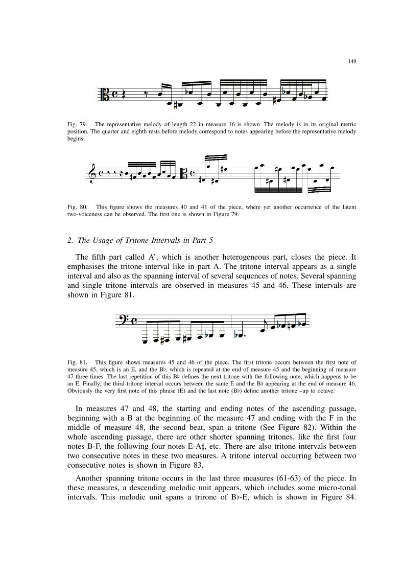
149

Fig. 79. The representative melody of length 22 in measure 16 is shown. The melody is in its original metricposition. The quarter and eighth rests before melody correspond to notes appearing before the representative melodybegins.

Fig. 80. This figure shows the measures 40 and 41 of the piece, where yet another occurrence of the latenttwo-voiceness can be observed. The first one is shown in Figure 79.

2. The Usage of Tritone Intervals in Part 5

The fifth part called A’, which is another heterogeneous part, closes the piece. Itemphasises the tritone interval like in part A. The tritone interval appears as a singleinterval and also as the spanning interval of several sequences of notes. Several spanningand single tritone intervals are observed in measures 45 and 46. These intervals areshown in Figure 81.

Fig. 81. This figure shows measures 45 and 46 of the piece. The first tritone occurs between the first note ofmeasure 45, which is an E, and the B[, which is repeated at the end of measure 45 and the beginning of measure47 three times. The last repetition of this B[ defines the next tritone with the following note, which happens to bean E. Finally, the third tritone interval occurs between the same E and the B[ appearing at the end of measure 46.Obviously the very first note of this phrase (E) and the last note (B[) define another tritone –up to octave.

In measures 47 and 48, the starting and ending notes of the ascending passage,beginning with a B at the beginning of the measure 47 and ending with the F in themiddle of measure 48, the second beat, span a tritone (See Figure 82). Within thewhole ascending passage, there are other shorter spanning tritones, like the first fournotes B-F, the following four notes E-A], etc. There are also tritone intervals betweentwo consecutive notes in these two measures. A tritone interval occurring between twoconsecutive notes is shown in Figure 83.

Another spanning tritone occurs in the last three measures (61-63) of the piece. Inthese measures, a descending melodic unit appears, which includes some micro-tonalintervals. This melodic unit spans a trirone of B[-E, which is shown in Figure 84.

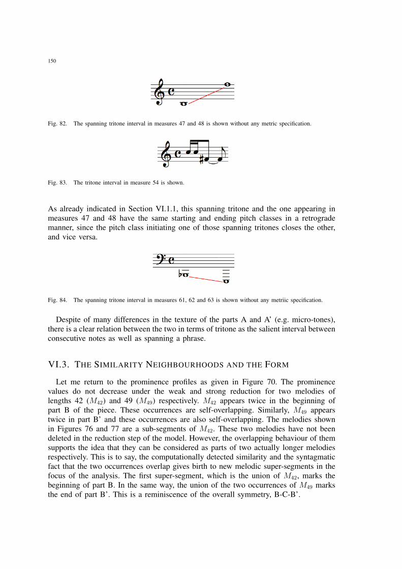
150

Fig. 82. The spanning tritone interval in measures 47 and 48 is shown without any metric specification.

Fig. 83. The tritone interval in measure 54 is shown.

As already indicated in Section VI.1.1, this spanning tritone and the one appearing inmeasures 47 and 48 have the same starting and ending pitch classes in a retrogrademanner, since the pitch class initiating one of those spanning tritones closes the other,and vice versa.

Fig. 84. The spanning tritone interval in measures 61, 62 and 63 is shown without any metriic specification.

Despite of many differences in the texture of the parts A and A’ (e.g. micro-tones),there is a clear relation between the two in terms of tritone as the salient interval betweenconsecutive notes as well as spanning a phrase.

VI.3. THE SIMILARITY NEIGHBOURHOODS AND THE FORM

Let me return to the prominence profiles as given in Figure 70. The prominencevalues do not decrease under the weak and strong reduction for two melodies oflengths 42 (M42) and 49 (M49) respectively. M42 appears twice in the beginning ofpart B of the piece. These occurrences are self-overlapping. Similarly, M49 appearstwice in part B’ and these occurrences are also self-overlapping. The melodies shownin Figures 76 and 77 are a sub-segments of M42. These two melodies have not beendeleted in the reduction step of the model. However, the overlapping behaviour of themsupports the idea that they can be considered as parts of two actually longer melodiesrespectively. This is to say, the computationally detected similarity and the syntagmaticfact that the two occurrences overlap gives birth to new melodic super-segments in thefocus of the analysis. The first super-segment, which is the union of M42, marks thebeginning of part B. In the same way, the union of the two occurrences of M49 marksthe end of part B’. This is a reminiscence of the overall symmetry, B-C-B’.

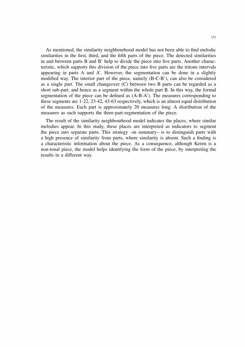
151

As mentioned, the similarity neighbourhood model has not been able to find melodicsimilarities in the first, third, and the fifth parts of the piece. The detected similaritiesin and between parts B and B’ help to divide the piece into five parts. Another charac-teristic, which supports this division of the piece into five parts are the tritone intervalsappearing in parts A and A’. However, the segmentation can be done in a slightlymodified way. The interior part of the piece, namely (B-C-B’), can also be consideredas a single part. The small changeover (C) between two B parts can be regarded as ashort sub-part, and hence as a segment within the whole part B. In this way, the formalsegmentation of the piece can be defined as (A-B-A’). The measures corresponding tothese segments are 1-22, 23-42, 43-63 respectively, which is an almost equal distributionof the measures. Each part is approximately 20 measures long. A distribution of themeasures as such supports the three-part-segmentation of the piece.

The result of the similarity neighbourhood model indicates the places, where similarmelodies appear. In this study, these places are interpreted as indicators to segmentthe piece into separate parts. This strategy –in summary– is to distinguish parts witha high presence of similarity from parts, where similarity is absent. Such a finding isa characteristic information about the piece. As a consequence, although Keren is anon-tonal piece, the model helps identifying the form of the piece, by interpreting theresults in a different way.

152

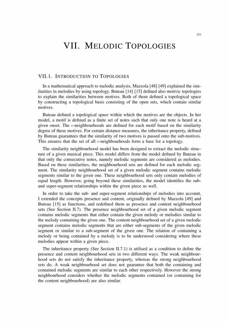
153

VII. MELODIC TOPOLOGIES

VII.1. INTRODUCTION TO TOPOLOGIES

In a mathematical approach to melodic analysis, Mazzola [48] [49] explained the sim-ilarities in melodies by using topology. Buteau [14] [15] defined also motivic topologiesto explain the similarities between motives. Both of them defined a topological spaceby constructing a topological basis consisting of the open sets, which contain similarmotives.

Buteau defined a topological space within which the motives are the objects. In hermodel, a motif is defined as a finite set of notes such that only one note is heard at agiven onset. The ε-neighbourhoods are defined for each motif based on the similaritydegree of these motives. For certain distance measures, the inheritance property, definedby Buteau guarantees that the similarity of two motives is passed onto the sub-motives.This ensures that the set of all ε-neighbourhoods form a base for a topology.

The similarity neighbourhood model has been designed to extract the melodic struc-ture of a given musical piece. This model differs from the model defined by Buteau inthat only the consecutive notes, namely melodic segments are considered as melodies.Based on these similarities, the neighbourhood sets are defined for each melodic seg-ment. The similarity neighbourhood set of a given melodic segment contains melodicsegments similar to the given one. These neighbourhood sets only contain melodies ofequal length. However, going beyond these similarities, the model identifies the sub-and super-segment relationships within the given piece as well.

In order to take the sub- and super-segment relationships of melodies into account,I extended the concepts presence and content, originally defined by Mazzola [49] andButeau [15] as functions, and redefined them as presence and content neighbourhoodsets (See Section II.7). The presence neighbourhood set of a given melodic segmentcontains melodic segments that either contain the given melody or melodies similar tothe melody containing the given one. The content neighbourhood set of a given melodicsegment contains melodic segments that are either sub-segments of the given melodicsegment or similar to a sub-segment of the given one. The relation of containing amelody or being contained by a melody is to be understood considering where thesemelodies appear within a given piece.

The inheritance property (See Section II.7.1) is utilised as a condition to define thepresence and content neighbourhood sets in two different ways. The weak neighbour-hood sets do not satisfy the inheritance property, whereas the strong neighbourhoodsets do. A weak neighbourhood set does not guarantee that both the containing andcontained melodic segments are similar to each other respectively. However the strongneighbourhood considers whether the melodic segments contained (or containing forthe content neighbourhood) are also similar.

154

These segment relationships are then utilised to eliminate those, which are identifiedto be redundant for this piece. The reduction step emphasises the remaining melodiesthat are of key importance in a given piece.

The similarity neighbourhood model, explained in detail in Chapter II, is inspired bytopology. For this reason, topological terminology is used for some musical and musictheoretical relations. However it is not a topological model in the strict mathematicalsense. Therefore, analysing which properties of a topology, both the model and theobtained results possess may hold important insights for interpreting the results. In thischapter, the topological features of the similarity neighbourhood model are investigatedfrom a theoretical viewpoint, in order to figure out under which conditions the collectionof the results yielded by the model define a topology. These features are then examinedfor the example of the two-voice inventions.

VII.2. MELODIC TOPOLOGIES

1. Basics of Topology

Topology is a branch of mathematics, which deals with the similarities of mathemat-ical objects. It is a collection of open or closed sets, also containing the empty set andthe entire space and is closed under the operations union and finite intersection.

Neighbourhood is one of the central concepts in a topological space. Generally, aneighbourhood N of a point x is a set, within which one can move, without leavingthe set.

Definition 7.1: A neighbourhood of a point x is any set that contains an open setcontaining x.

The neighbourhood system at x consists of all neighbourhoods of x. A topology canbe determined by a set of axioms concerning all neighbourhood systems.

Definition 7.2: A topological space is a set X together with a collection T of subsetsof X satisfying the following axioms:

1) The empty set and X are in T .2) The union of any collection of sets in T is also in T .3) The intersection of any pair of sets in T is also in T .

In many cases, large neighbourhoods are not necessary for a topology. The so calledbasic neighbourhoods are sufficient to define a topology. One can make use of theseneighbourhoods to obtain large neighbourhoods by uniting the basic neighbourhoods.The collection of such basic neighbourhoods is called a topological base, which isformally defined in the following [13]:

Definition 7.3: A base for the neighbourhoods at x ∈ X is a set B(x) of neigh-bourhoods of x such that if N is a neighbourhood of x then N contains some B ofB(x).

155

According to this definition, every neighbourhood of a topology should be able to bedefined as a union of an arbitrary number of neighbourhoods within the base.

2. Melodic Topologies on Prototypes

In order to identify the similarities between melodies, I basically investigated threedifferent distance measures, namely the Euclidean distance, the edit distance and thecorrelation coefficient. The first two distance measures define a metric, however thecorrelation coefficient does not. All metric spaces define automatically a topology [13].So the first two distance measures that I used define already a topology.

However the correlation coefficient does not automatically define a topology, becauseit is not a metric. For a distance measure to be a metric, three conditions [24] must besatisfied:

1) ρ(x, y) is a finite real number for every pair (x, y).2) ρ(x, y) = 0 if and only if x = y.3) ρ(x, z) <= ρ(x, y) + ρ(y, z).

The Euclidean distance and the edit distance satisfy all three conditions. The proofscan be found in a range sources. Therefore I do not repeat them here. However thecorrelation coefficient does satisfy neither the identity (2) nor the triangular inequality(3). The second condition is not satisfied simply because if x = y, then ρ(x, y) = 1.However, it is possible to convert the formula so that this condition is satisfied, namelyd(x, y) = 1−ρ(x, y) or d(x, y) = 1−ρ2(x, y). Even in this form, however, the coefficientof correlation does not satisfy the triangular inequality.

Consequently, the correlation coefficient, does not define a metric. Therefore thesimilarity neighbourhood sets constructed by using the correlation coefficient do notautomatically define a topological base. In order to define a topological base, someproperties are needed so that the similarity neighbourhood model with the correlationcoefficient defines a topological base.

In the following sections, I investigate the correlation coefficient in detail, and showunder which conditions the presence and content neighbourhood sets for the connectivityclasses define topological bases. In these investigations, the significance threshold isset to zero, so that not only the prototypical connectivity classes but also the non-prototypical connectivity classes can be considered.

3. Topologies on Connectivity Classes

The connectivity classes are the sets, which unite all the similarity neighbourhoodsof the first, second- up to nth order similar melodies. In this section, the connectivityclasses are investigated, in order to assess, whether they define a topological base [7].Recall that the basic neighbourhoods are united to define other neighbourhood setswithin a topology. So the intersections of the basic neighbourhoods will be basic

156

neighbourhoods as well. Considering this fact, the following defines the topologicalbase for the connectivity classes:

Theorem 3: The collection {Enc (M)} of the connectivity classes for a given musical

piece M defines a base for a topology τ on the set {m|m ∈ M}.

Proof: Due to Corollary 2.1, the intersection of any number of connectivity classesis empty. The empty set and the whole collection is automatically within the base. Sothe proof is done.

However, the topology defined in Theorem 3 yields neither mathematically nor musictheoretically interesting results. The fact that the intersections are always empty doesnot bring any new structure to the results. However, in the following sections othertopologies will be defined, where the intersections of the open sets will not be empty.In those topologies I will investigate, under which conditions the intersections of thepresence as well as the content neighbourhood sets for the connectivity classes areincluded within one another.

4. Topologies on Presence Neighbourhood Sets

The presence neighbourhood sets of the connectivity classes define a topological baseas well.

Theorem 4: The collection {PEq(Enc (M))} of presence neighbourhood sets for the

connectivity classes of a given musical piece M defines a base for a topology τ on theset {m|m ∈ M}, if and only if the inheritance property is satisfied.

Proof: It is enough to show that given the connectivity classes Enc (M) and En′

d (M)and a melodic segment m′ ∈ En′

d (M) such that m′ ∈ PEq(Enc (M)), the following is

true:PEq(E

n′

d (M)) ⊂ PEq(Enc (M)).

If the inheritance property holds, there exists a melodic segment m′ such that m′ =m′n

i and due to Corollary 2.3, m′ ∈ Enc (M).

Suppose that there exists a melodic segment m′′ ∈ En′′u (M) such that m′′ ∈ PEq(E

n′

d (M)).This means that there exists a melodic segment m′′ such that m′′ = m′′n′

j and due toCorollary 2.3, m′′ ∈ En′

d (M).

In the same way, due to Corollary 2.3, there should exist another melodic segmento = m′′n

i such that o ∈ Enc (M). So

PEqn′′

(Enc (M)) ⊃ En′′

u (M) ⊂ PEqn′′

(En′

d (M)).

157

The inheritance property ensures that the melody o exists. If the inheritance propertydoes not hold, this cannot be assumed. Therefore if the inheritance property is notsatisfied, the proof is incomplete.

Based on Corollary 2.1 the intersection of the presence neighbourhood for the con-nectivity classes are either empty sets or they contain one another. So the set of allpresence neighbourhood sets of the connectivity classes define a topological base.

5. Topologies on Content Neighbourhood Sets

A similar topological investigation for the content neighbourhood sets for the con-nectivity classes yields similar results.

Theorem 5: The collection {CEq(Enc (M))} of content neighbourhood sets of the

connectivity classes for a given musical piece M defines a base for a topology τ onthe set {m|m ∈ M}, if and only if the inheritance property is satisfied.

Proof: The proof of this theorem is similar to Theorem 4.

6. Is the Inheritance Property Satisfied?

The presence and content neighbourhood sets for connectivity classes consist ofconnectivity classes or unions of them. Corollary 2.1 indicates that the intersectionof connectivity classes is empty. Hence, intersections of any presence or content neigh-bourhood sets for the connectivity classes are either empty or a connectivity class or theunion of connectivity classes. Considering the situation for the presence neighbourhoodsets for the connectivity classes, there are three cases:

Case 1:

P nEq(E

nc (M)) = En

j (M),P n

Eq(End (M)) = En

i (M),P n

Eq(Enc (M)) ∩ P n

Eq(End (M)) = ∅.

In this case, the inheritance property is not violated. Two connectivity classes withoutany shared similarities have an empty intersection of their presence neighbourhood sets.

Case 2:

P nEq(E

nc ) = En

i (M) ∪ Enj (M),

P nEq(E

nd ) = En

i (M),P n

Eq(Enc ) ∩ P n

Eq(End ) = En

i (M).

This case violates the inheritance property. Two connectivity classes have the sameconnectivity class in their presence neighbourhood sets. This means that two similarmelodies are contained in two dissimilar melodies. However, in this particular case,

158

the intersection of the presence neighbourhood set is included in another presenceneighbourhood set.

Case 3:

P nEq(E

nc ) = En

i (M) ∪ Enj (M),

P nEq(E

nd ) = En

i (M) ∪ Enii(M),

P nEq(E

nc ) ∩ P n

Eq(End ) = En

i (M).

The third case violates the inheritance property as well. However, in this case, theintersection of these two presence neighbourhood sets is not included in another presenceneighbourhood set. Therefore this last constellation does not define a topology. Howeverthe other two constellations do not violate the axioms defining a topology, even-thoughthe second case violates the inheritance property. The second case is still a special case,which should not be considered a general possibility that occurs frequently. Theorems 4and 5 show that the collections of the presence as well as the content neighbourhood setsfor the connectivity classes form a base for a topology as long as the inheritance propertyis satisfied. Hence the inheritance property is the mathematically proven property, whichis necessary to define a topological base. However, it should be clarified, under whichconditions the inheritance property is satisfied. The problem can be formulated in thefollowing way:

Question 7.1: Suppose there exist two melodies m1 and m2 such that

m1, m2 ∈ Enc (M) where ||m1|| = ||m2|| = n,

and further suppose these melodies have two sub-melodies m1 and m2 such that

m1 = m1n1 , m2 = m2

n1 .

Does m1 ∈ End (M) imply m2 ∈ En

d (M)?

In general, if two melodies m and m′ are in the same connectivity class, there shouldbe a sequence of melodies

(m,m1, m2, . . . ,mp, m′)

such that

d(m, m1) < R,

d(m1, m2) < R,

. . .

d(mp, m′) < R,

where R is the similarity threshold. However, I dispense with higher-order similarities,and answer Question 7.1 for the first-order similarities only.

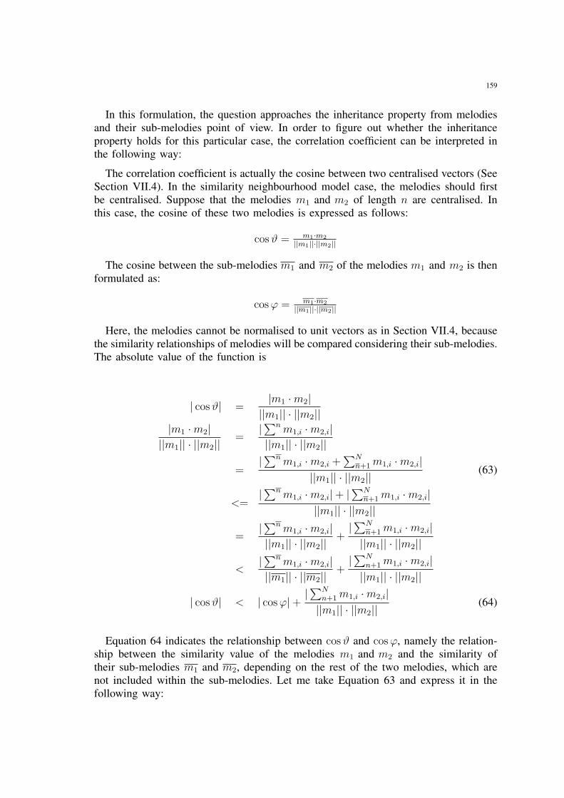
159

In this formulation, the question approaches the inheritance property from melodiesand their sub-melodies point of view. In order to figure out whether the inheritanceproperty holds for this particular case, the correlation coefficient can be interpreted inthe following way:

The correlation coefficient is actually the cosine between two centralised vectors (SeeSection VII.4). In the similarity neighbourhood model case, the melodies should firstbe centralised. Suppose that the melodies m1 and m2 of length n are centralised. Inthis case, the cosine of these two melodies is expressed as follows:

cos ϑ = m1·m2

||m1||·||m2||

The cosine between the sub-melodies m1 and m2 of the melodies m1 and m2 is thenformulated as:

cos ϕ = m1·m2

||m1||·||m2||

Here, the melodies cannot be normalised to unit vectors as in Section VII.4, becausethe similarity relationships of melodies will be compared considering their sub-melodies.The absolute value of the function is

| cos ϑ| =|m1 ·m2|

||m1|| · ||m2|||m1 ·m2|

||m1|| · ||m2||=

|∑n m1,i ·m2,i|||m1|| · ||m2||

=|∑n m1,i ·m2,i +

∑Nn+1 m1,i ·m2,i|

||m1|| · ||m2||(63)

<=|∑n m1,i ·m2,i|+ |

∑Nn+1 m1,i ·m2,i|

||m1|| · ||m2||

=|∑n m1,i ·m2,i|||m1|| · ||m2||

+|∑N

n+1 m1,i ·m2,i|||m1|| · ||m2||

<|∑n m1,i ·m2,i|||m1|| · ||m2||

+|∑N

n+1 m1,i ·m2,i|||m1|| · ||m2||

| cos ϑ| < | cos ϕ|+|∑N

n+1 m1,i ·m2,i|||m1|| · ||m2||

(64)

Equation 64 indicates the relationship between cos ϑ and cos ϕ, namely the relation-ship between the similarity value of the melodies m1 and m2 and the similarity oftheir sub-melodies m1 and m2, depending on the rest of the two melodies, which arenot included within the sub-melodies. Let me take Equation 63 and express it in thefollowing way:

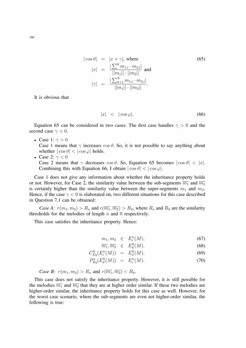
160

| cos ϑ| = |x + γ|, where (65)

|x| =|∑n m1,i ·m2,i|||m1|| · ||m2||

and

|γ| =|∑N

n+1 m1,i ·m2,i|||m1|| · ||m2||

.

It is obvious that

|x| < | cos ϕ|. (66)

Equation 65 can be considered in two cases: The first case handles γ > 0 and thesecond case γ < 0.

• Case 1: γ > 0Case 1 means that γ increases cos ϑ. So, it is not possible to say anything aboutwhether | cos ϑ| < | cos ϕ| holds.

• Case 2: γ < 0Case 2 means that γ decreases cos ϑ. So, Equation 65 becomes | cos ϑ| < |x|.Combining this with Equation 66, I obtain | cos ϑ| < | cos ϕ|.

Case 1 does not give any information about whether the inheritance property holdsor not. However, for Case 2, the similarity value between the sub-segments m1 and m2

is certainly higher than the similarity value between the super-segments m1 and m2.Hence, if the case γ < 0 is elaborated on, two different situations for this case describedin Question 7.1 can be obtained:

Case A: r(m1, m2) > Rn and r(m1, m2) > Rn, where Rn and Rn are the similaritythresholds for the melodies of length n and n respectively.

This case satisfies the inheritance property. Hence:

m1, m2 ∈ Enc (M), (67)

m1, m2 ∈ End (M). (68)

CnEq(E

nc (M)) = En

d (M), (69)

P nEq(E

nd (M)) = En

c (M). (70)

Case B: r(m1, m2) > Rn and r(m1, m2) < Rn.

This case does not satisfy the inheritance property. However, it is still possible forthe melodies m1 and m2 that they are at higher order similar. If these two melodies arehigher-order similar, the inheritance property holds for this case as well. However, forthe worst case scenario, where the sub-segments are even not higher-order similar, thefollowing is true:

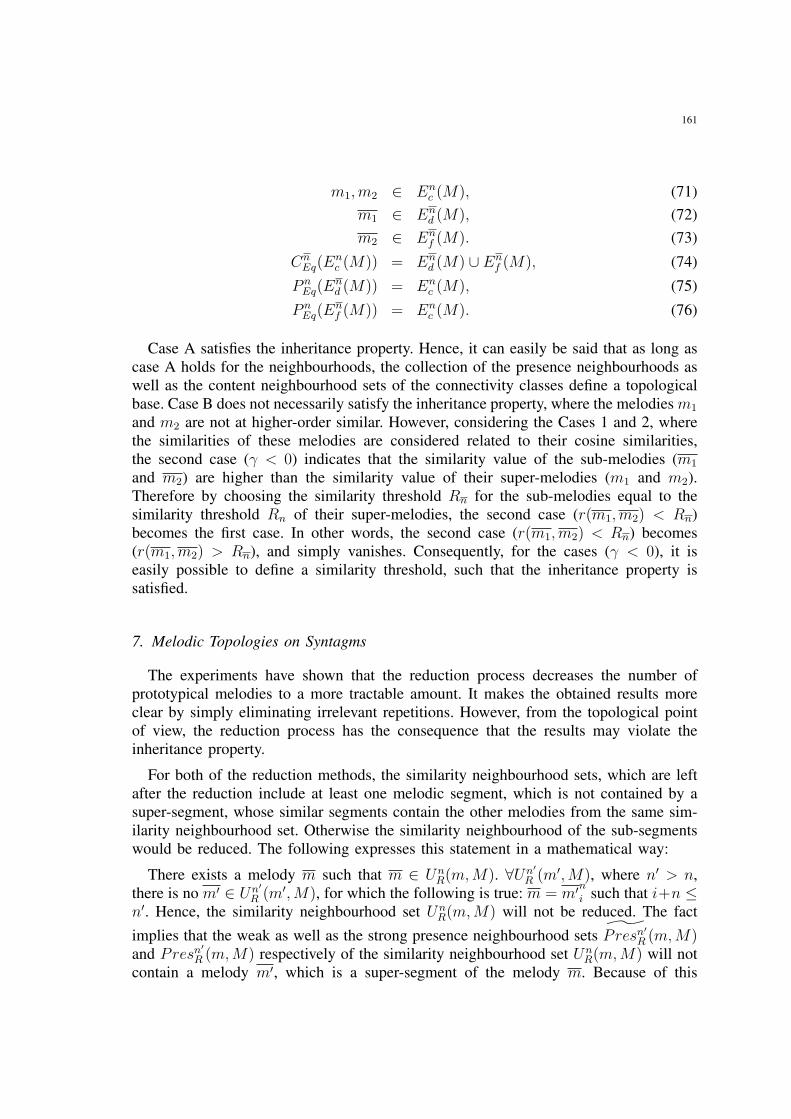
161

m1, m2 ∈ Enc (M), (71)

m1 ∈ End (M), (72)

m2 ∈ Enf (M). (73)

CnEq(E

nc (M)) = En

d (M) ∪ Enf (M), (74)

P nEq(E

nd (M)) = En

c (M), (75)

P nEq(E

nf (M)) = En

c (M). (76)

Case A satisfies the inheritance property. Hence, it can easily be said that as long ascase A holds for the neighbourhoods, the collection of the presence neighbourhoods aswell as the content neighbourhood sets of the connectivity classes define a topologicalbase. Case B does not necessarily satisfy the inheritance property, where the melodies m1

and m2 are not at higher-order similar. However, considering the Cases 1 and 2, wherethe similarities of these melodies are considered related to their cosine similarities,the second case (γ < 0) indicates that the similarity value of the sub-melodies (m1

and m2) are higher than the similarity value of their super-melodies (m1 and m2).Therefore by choosing the similarity threshold Rn for the sub-melodies equal to thesimilarity threshold Rn of their super-melodies, the second case (r(m1, m2) < Rn)becomes the first case. In other words, the second case (r(m1, m2) < Rn) becomes(r(m1, m2) > Rn), and simply vanishes. Consequently, for the cases (γ < 0), it iseasily possible to define a similarity threshold, such that the inheritance property issatisfied.

7. Melodic Topologies on Syntagms

The experiments have shown that the reduction process decreases the number ofprototypical melodies to a more tractable amount. It makes the obtained results moreclear by simply eliminating irrelevant repetitions. However, from the topological pointof view, the reduction process has the consequence that the results may violate theinheritance property.

For both of the reduction methods, the similarity neighbourhood sets, which are leftafter the reduction include at least one melodic segment, which is not contained by asuper-segment, whose similar segments contain the other melodies from the same sim-ilarity neighbourhood set. Otherwise the similarity neighbourhood of the sub-segmentswould be reduced. The following expresses this statement in a mathematical way:

There exists a melody m such that m ∈ UnR(m, M). ∀Un′

R (m′, M), where n′ > n,there is no m′ ∈ Un′

R (m′, M), for which the following is true: m = m′ni such that i+n ≤

n′. Hence, the similarity neighbourhood set UnR(m,M) will not be reduced. The fact

implies that the weak as well as the strong presence neighbourhood sets P resn′R (m, M)

and Presn′R (m, M) respectively of the similarity neighbourhood set Un

R(m,M) will notcontain a melody m′, which is a super-segment of the melody m. Because of this

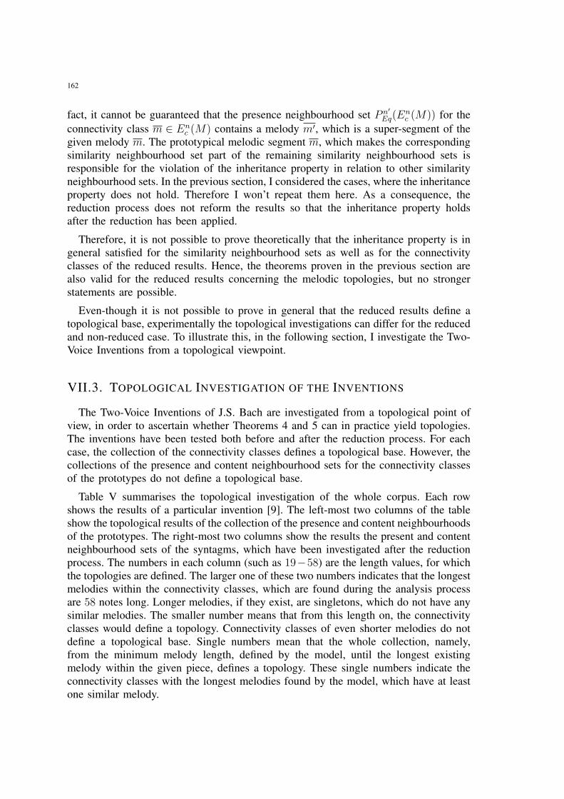
162

fact, it cannot be guaranteed that the presence neighbourhood set P n′Eq(E

nc (M)) for the

connectivity class m ∈ Enc (M) contains a melody m′, which is a super-segment of the

given melody m. The prototypical melodic segment m, which makes the correspondingsimilarity neighbourhood set part of the remaining similarity neighbourhood sets isresponsible for the violation of the inheritance property in relation to other similarityneighbourhood sets. In the previous section, I considered the cases, where the inheritanceproperty does not hold. Therefore I won’t repeat them here. As a consequence, thereduction process does not reform the results so that the inheritance property holdsafter the reduction has been applied.

Therefore, it is not possible to prove theoretically that the inheritance property is ingeneral satisfied for the similarity neighbourhood sets as well as for the connectivityclasses of the reduced results. Hence, the theorems proven in the previous section arealso valid for the reduced results concerning the melodic topologies, but no strongerstatements are possible.

Even-though it is not possible to prove in general that the reduced results define atopological base, experimentally the topological investigations can differ for the reducedand non-reduced case. To illustrate this, in the following section, I investigate the Two-Voice Inventions from a topological viewpoint.

VII.3. TOPOLOGICAL INVESTIGATION OF THE INVENTIONS

The Two-Voice Inventions of J.S. Bach are investigated from a topological point ofview, in order to ascertain whether Theorems 4 and 5 can in practice yield topologies.The inventions have been tested both before and after the reduction process. For eachcase, the collection of the connectivity classes defines a topological base. However, thecollections of the presence and content neighbourhood sets for the connectivity classesof the prototypes do not define a topological base.

Table V summarises the topological investigation of the whole corpus. Each rowshows the results of a particular invention [9]. The left-most two columns of the tableshow the topological results of the collection of the presence and content neighbourhoodsof the prototypes. The right-most two columns show the results the present and contentneighbourhood sets of the syntagms, which have been investigated after the reductionprocess. The numbers in each column (such as 19−58) are the length values, for whichthe topologies are defined. The larger one of these two numbers indicates that the longestmelodies within the connectivity classes, which are found during the analysis processare 58 notes long. Longer melodies, if they exist, are singletons, which do not have anysimilar melodies. The smaller number means that from this length on, the connectivityclasses would define a topology. Connectivity classes of even shorter melodies do notdefine a topological base. Single numbers mean that the whole collection, namely,from the minimum melody length, defined by the model, until the longest existingmelody within the given piece, defines a topology. These single numbers indicate theconnectivity classes with the longest melodies found by the model, which have at leastone similar melody.

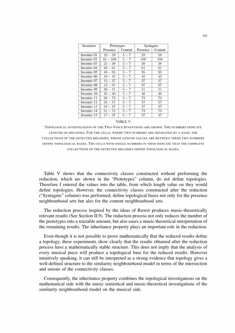
163

Invention Prototypes SyntagmsPresence Content Presence Content

Inventio 01 19 − 58 5 − 7 58 58Inventio 02 42 − 108 5 − 7 108 108Inventio 03 21 − 38 5 − 7 38 38Inventio 04 36 − 61 5 − 7 61 61Inventio 05 48 − 95 5 − 7 95 95Inventio 06 19 − 45 5 − 7 45 45Inventio 07 15 − 37 5 − 7 37 37Inventio 08 12 − 97 5 − 7 97 97Inventio 09 30 − 51 5 − 7 51 51Inventio 10 25 − 40 5 − 7 40 40Inventio 11 26 − 73 5 − 7 73 73Inventio 12 32 − 57 5 − 7 57 57Inventio 13 18 − 37 5 − 7 37 37Inventio 14 51 − 73 5 − 7 73 73Inventio 15 17 − 37 5 − 7 37 37

TABLE V

TOPOLOGICAL INVESTIGATION OF THE TWO-VOICE INVENTIONS ARE SHOWN. THE NUMBERS INDICATE

LENGTHS OF MELODIES. FOR THE CELLS, WHERE TWO NUMBERS ARE SEPARATED BY A DASH, THE

COLLECTIONS OF THE DETECTED MELODIES, WHOSE LENGTH VALUES ARE BETWEEN THESE TWO NUMBERS

DEFINE TOPOLOGICAL BASES. THE CELLS WITH SINGLE NUMBERS IN THEM INDICATE THAT THE COMPLETE

COLLECTIONS OF THE DETECTED MELODIES DEFINE TOPOLOGICAL BASES.

Table V shows that the connectivity classes constructed without performing thereduction, which are shown in the “Prototypes” column, do not define topologies.Therefore I entered the values into the table, from which length value on they woulddefine topologies. However, the connectivity classes constructed after the reduction(“Syntagms” column) was performed, define topological bases not only for the presenceneighbourhood sets but also for the content neighbourhood sets.

The reduction process inspired by the ideas of Ruwet produces music-theoreticallyrelevant results (See Section II.9). The reduction process not only reduces the number ofthe prototypes into a tractable amount, but also eases a music-theoretical interpretation ofthe remaining results. The inheritance property plays an important role in the reduction.

Even-though it is not possible to prove mathematically that the reduced results definea topology, these experiments show clearly that the results obtained after the reductionprocess have a mathematically stable structure. This does not imply that the analysis ofevery musical piece will produce a topological base for the reduced results. Howeverintuitively speaking, it can still be interpreted as a strong evidence that topology gives awell-defined structure to the similarity neighbourhood model in terms of the intersectionand unions of the connectivity classes.

Consequently, the inheritance property combines the topological investigations on themathematical side with the music semiotical and music-theoretical investigations of thesimilarity neighbourhood model on the musical side.

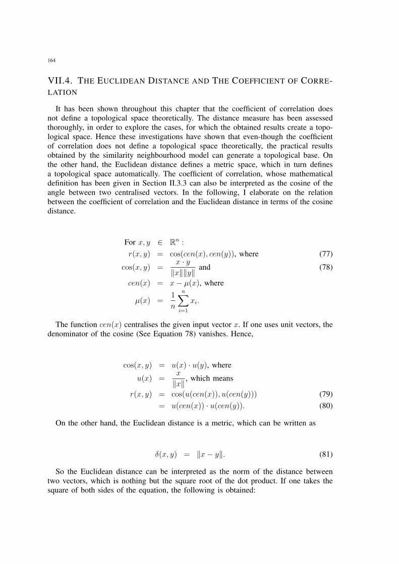
164

VII.4. THE EUCLIDEAN DISTANCE AND THE COEFFICIENT OF CORRE-LATION

It has been shown throughout this chapter that the coefficient of correlation doesnot define a topological space theoretically. The distance measure has been assessedthoroughly, in order to explore the cases, for which the obtained results create a topo-logical space. Hence these investigations have shown that even-though the coefficientof correlation does not define a topological space theoretically, the practical resultsobtained by the similarity neighbourhood model can generate a topological base. Onthe other hand, the Euclidean distance defines a metric space, which in turn definesa topological space automatically. The coefficient of correlation, whose mathematicaldefinition has been given in Section II.3.3 can also be interpreted as the cosine of theangle between two centralised vectors. In the following, I elaborate on the relationbetween the coefficient of correlation and the Euclidean distance in terms of the cosinedistance.

For x, y ∈ Rn :

r(x, y) = cos(cen(x), cen(y)), where (77)

cos(x, y) =x · y

‖x‖‖y‖and (78)

cen(x) = x− µ(x), where

µ(x) =1

n

n∑i=1

xi.

The function cen(x) centralises the given input vector x. If one uses unit vectors, thedenominator of the cosine (See Equation 78) vanishes. Hence,

cos(x, y) = u(x) · u(y), where

u(x) =x

‖x‖, which means

r(x, y) = cos(u(cen(x)), u(cen(y))) (79)= u(cen(x)) · u(cen(y)). (80)

On the other hand, the Euclidean distance is a metric, which can be written as

δ(x, y) = ‖x− y‖. (81)

So the Euclidean distance can be interpreted as the norm of the distance betweentwo vectors, which is nothing but the square root of the dot product. If one takes thesquare of both sides of the equation, the following is obtained:

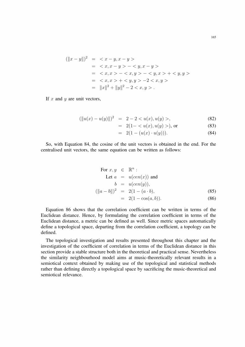
165

(‖x− y‖)2 = < x− y, x− y >

= < x, x− y > − < y, x− y >

= < x, x > − < x, y > − < y, x > + < y, y >

= < x, x > + < y, y > −2 < x, y >

= ‖x‖2 + ‖y‖2 − 2 < x, y > .

If x and y are unit vectors,

(‖u(x)− u(y)‖)2 = 2− 2 < u(x), u(y) >, (82)= 2(1− < u(x), u(y) >), or (83)= 2(1− (u(x) · u(y))). (84)

So, with Equation 84, the cosine of the unit vectors is obtained in the end. For thecentralised unit vectors, the same equation can be written as follows:

For x, y ∈ Rn :

Let a = u(cen(x)) andb = u(cen(y)),

(‖a− b‖)2 = 2(1− (a · b), (85)= 2(1− cos(a, b)). (86)

Equation 86 shows that the correlation coefficient can be written in terms of theEuclidean distance. Hence, by formulating the correlation coefficient in terms of theEuclidean distance, a metric can be defined as well. Since metric spaces automaticallydefine a topological space, departing from the correlation coefficient, a topology can bedefined.

The topological investigation and results presented throughout this chapter and theinvestigation of the coefficient of correlation in terms of the Euclidean distance in thissection provide a stable structure both in the theoretical and practical sense. Neverthelessthe similarity neighbourhood model aims at music-theoretically relevant results in asemiotical context obtained by making use of the topological and statistical methodsrather than defining directly a topological space by sacrificing the music-theoretical andsemiotical relevance.

166

167

VIII. CONCLUSION

VIII.1. GENERAL CONCLUSIONS

The similarity neighbourhood model is a simple yet powerful model for performingparadigmatic melodic analysis of musical pieces. The aim of the model is to helpidentifying the melodic structure of a given piece. The similarity neighbourhoods ofthe prominent melodies, the associated connectivity components and the sub-segmentrelationships can be interpreted directly without using any complex post-processingmethods such as discussed in Chapters IV and VI. Furthermore, they can be used as inputto perform additional analysis from different viewpoints. A syntagmatic analysis can beperformed in a subsequent step by considering the interaction of the melodies identifiedby the method with their environment. Harmonic analysis is another analysis method,which can be used for studying the solidarity of melodic variation with harmonicprogression.

From theoreticians viewpoint, the theoretical basis of the similarity neighbourhoodmodel is comparable to other theoretical approaches. The theory underlying this studyis based on music-theoretical facts and on the representation of these facts by usingmathematical, semiotical and computational building blocks. Mathematics has been usedfor the representation of musical concepts, and for identifying the similarities betweenthem. These similarities have been incorporated for identifying the prominent melodieswithin a given piece, and for investigating the sub-segment relationships from a semioticviewpoint. In the realisation of the theory, computational methods and clever algorithmshave been used, which made the whole theory applicable for testing the performance.Hence, the analyst makes use of the applicability of the method on pieces of differentmusical styles. The obtained results are justifiable with respect to the music-theoreticalanalysis of the same piece. Additionally, the results can be compared to the resultsyielded by other analysis models.

Especially from the music-theoretical point of view, it is possible to legitimate the re-sults of the model with the results of the music-theoretical analysis. However, this studydoes not aim at performing a melodic analysis automatically, in a music-theoretical way.The aim of this research is rather to bridge the traditional approaches with mathematicaland semiotic ideas in a computational framework. Therefore it is important to observe,where these approaches show analogies, and where they diverge from each other.

A cause of the divergence between the traditional music theory and the paradigmaticapproach used in this study is that the paradigmatic approach does not take the relationsof the melodies with their environment into account within a given piece, where thetraditional music theory would bring issues of form, harmony and metric organisationinto play.

The encouraging results, I obtained from the tests (See Chapters IV and VI) gives

168

me the right to claim that the similarity neighbourhood model is a practical alternativeto the complicated approaches of Mazzola [49], Buteau [14] [15] and Nestke [60] dueto the practicality and the applicability of the model onto different styles of musicalpieces. However, instead of conceiving my approach only as an exclusive alternativeto these approaches, I propose that my methods can be suitably integrated with thesemethods into a further research in a broadened field.

1. Building Blocks

The similarity neighbourhood model is developed to be a paradigmatic model incor-porating mathematical and semiotical approaches in a computer aided framework. It isa hierarchical model, where representation of melodies underlies the whole hierarchy.

Representation of Melodies: In the similarity neighbourhood model, a melodyis defined to be a tone sequence of consecutive notes from the same voice (melodicsegment) without any metrical information. The decision to restrict the model to melodicsegments not only decreased the time needed to process a piece, but also simplified theinterpretation of the results of the model from the music-theoretical point of view.Furthermore, the model identifies the melodies as similar, as long as the tone sequenceis kept similar, without considering the rhythmic changes within the melody. In this way,I labelled the rhythmic alterations, augmentations and diminutions as similar, withoutidentifying them. Finally, the model cannot recognise similarities between melodicprogressions moving from one voice to another within the given piece.

The model is able to grasp the similarity of melodies, which are associated withmusic-theoretical relations such as alterations (proximity), diatonic and chromatic trans-positions and inversion (symmetry). All these variation techniques occur in many mu-sical styles. Tests performed for several different styles show that the model can extractthese variations in musical pieces composed in different styles as well. The similarityby proximity is preferred for spotting similarities between tone sequences. Similarity bysymmetry can easily be built into the present software but in view of high computationalcosts, I dispense with this possibility.

Distance Measure: In order to identify similarity by proximity the correlationcoefficient is used in the model. Due to the fact that correlation coefficient can onlybe applied onto equal length melodies, the model cannot identify variations obtainedby inserting or deleting a note. Hence, given a melody within a given musical piece,similar, equal length melodies are extracted and collected in a neighbourhood set, whichis called the similarity neighbourhood set of the given melody.

Connectivity of Similarity: Similarity is a symmetric relation. Therefore, two sim-ilar melodies contain each other within their similarity neighbourhood sets. Intuitivelyspeaking, several other melodies are contained in these neighbourhood sets as well.Hence, combining these sets in a larger set has two-fold advantages compared to thesimilarity neighbourhood sets. On the one hand, collecting the similarity neighbourhoodsets containing same melodies reduces the number of similarity neighbourhood setsand in turn the number of results. On the other hand, similarities of higher degree

169

can be observed as well, by simply tracking the connections between the similarityneighbourhood sets containing similar melodies. Hence, the connectivity of the similaritycan reveal the development of a particular melody throughout the given piece completely.

Sub-Segment Relationships: Since the distance measure can measure only thesimilarities between equal length melodies, the similarity neighbourhood set of a givenmelody contains only equal length melodies. The relationships between different lengthmelodies cannot be measured in the same way. Therefore, in the next level of the modelhierarchy, these relationships are defined in terms of sub-segment relationships betweenmelodies.

Intuitively speaking, the sub-melodies of two similar melodies are similar as well. Inother words, the similarity of two melodies is inherited by their sub-melodies. In thesimilarity neighbourhood model, the inheritance property is defined as a bidirectionalproperty for explaining this relation not only from the melodies point of view, but alsofrom the sub-melodies viewpoint.

From the music-theoretical viewpoint, the relations between melodies of differentlength are explained, in order to understand, how the melodic material is introduced andused throughout a musical piece. The similarity neighbourhood sets and the bidirectionalinheritance property underlie the mechanism incorporated for explaining these relation-ships. The presence- and content neighbourhood sets are defined to be the collectionsof the similarity neighbourhood sets of the melodies, where one melody contains theother. These sets reveal how the melodic material is used within a given piece fromboth the sub-segments and super-segments perspective. The presented results indicatethe music theoretical relevance of these sets.

The bidirectional inheritance property is used as a condition to define the weak-and strong neighbourhoods for both presence- and content neighbourhood sets. Theneighbourhood sets that do not satisfy the inheritance property are called weak sets,whereas the neighbourhood sets that satisfy the inheritance property are called strongsets. Especially two melodic segments whose sub-segments are not similar or twomelodic sub-segments, whose super-segments are not similar, are interesting to analysethoroughly. The differences between the weak and strong neighbourhoods indicate thosesegments.

Reduction of Redundancy: The similarity neighbourhood model is by nature ex-haustive. The model generates the similarity neighbourhood set for each tone sequence,defined to be a melody. A sub-segment of a given melody appears exactly there, wherethe given melody appears as well. Hence the given melody and the sub-segment haveexactly the same similarity neighbourhood structure, unless the sub-segment appearsindividually at some other places within the piece as well. This situation causes aredundancy within the results, because a sub-segment (and its similarity neighbourhoodset in turn) appearing only within its super-segments does not contribute to how themelodic material is used music-theoretically throughout the piece. The similarity neigh-bourhood model makes use of the presence- and content neighbourhood sets in the nextmodel hierarchy, in order to eliminate those kinds of sub-segments and their similarityneighbourhood sets from the results. The so-called reduction procedure decreases the

170

amount of results, so that only music-theoretically interesting melodies remain. Asin defining the sub-segment relationships, the inheritance property is incorporated indetection and elimination of these redundant sub-segments. Depending on whether theinheritance property is satisfied or not, the reduction mechanisms are called strong- andweak reduction respectively.

One of the most important advantages of the reduction mechanism is that it reducesthe amount of the results, together with the connectivity mechanism, to a very tractableamount. Obviously, reduction eliminates generally relatively short melodies rather thanlong ones. Another important advantage of the reduction mechanism appears in thedifferences between the weak- and strong reduction mechanisms. Intuitively speaking,weak reduction reduces more than the strong reduction. This difference is significant forshort melodies. As melodies become longer, the differences between weak- and strongreduction disappear. From a certain length value on, these two reduction methods reducethe same melodic segments.

The differences between the weak and strong reductions are important, becausethey indicate melodies, which are removed by the weak reduction and not by thestrong reduction. Since the strong reduction obeys the inheritance property, all of theappearances of the melody to be reduced should be covered by a longer melody, whereasthe weak reduction only checks the number of appearances to reduce. Even-though thestrong reduction is music-theoretically motivated, the weak reduction depicts the generalview in a proper way as well. Therefore applying the weak reduction to see the generalmelodic structure is an acceptable alternative (or a preliminary step) to applying directlythe strong reduction onto the results.

Topological Investigation of the Model: Defining a topology [13] gives a preciseand general structure to the studies of proximity, namely similarities of objects. Topo-logical approach can be incorporated to study any kind of similarities.

The development of the similarity neighbourhood model does not aim at defininga topology. However, I investigated the circumstances under which the neighbourhoodsets define topological bases. Due to the non-metric nature of the correlation coefficient,the collection of the similarity neighbourhood sets does not define a topological base.However, in Chapter VII, it is shown that the collection of the connectivity classesdefines a topological base. Besides, it is discussed under which conditions the presenceand content neighbourhood sets for connectivity classes define a topological base. Therole of the inheritance property to form a topological base is discussed thoroughly.

Buteau [14] [15] and Mazzola [49] make use of the inheritance property to constructtopological bases. Their models define a topological base as long as the inheritanceproperty is satisfied. Some of the distance measures tested on these models obeythe inheritance property, which can be proven mathematically without considering themusical piece analysed. Hence, the generation of a topological base is granted for thesedistance measures. On the one hand, for the similarity neighbourhood set, the collectionof the results define a topological base for the cases where the inheritance property holds.However, it cannot be shown mathematically that the inheritance property is satisfiedfor all cases. On the other hand, the presence- as well as the content neighbourhood sets

171

for connectivity classes of the similarity neighbourhood model can define a topologicalbase depending on the given musical piece. The tests have shown that the collectionof the reduced results satisfy inheritance property for the whole corpus of Two-VoiceInventions. From the music-theoretical viewpoint, the reduction process inspired by theideas of Ruwet [67] produces music-theoretically relevant results. From a mathematicalperspective, the results obtained after the reduction process have a mathematically stablestructure. Even-though it cannot be proven mathematically that the results define atopological base, practical results are promising in the sense that reduction yields amusic-theoretically relevant results as well as brings a mathematical structure to theresults.

2. Approximation by Means of Genetic Algorithms

The similarity neighbourhood model extracts the prominence profile of a given pieceby traversing the piece for each melody. During this process, each melody is analysedto find the prototypes. This operation could be very time consuming especially forlong pieces. In order to accelerate the analysis process of a given piece without losingimportant information about the piece, the genetic algorithms are combined with thesimilarity neighbourhood model.

The genetic algorithms randomly select a population of melodies to analyse. Byselecting more prominent melodies and mutating them to generate new populations,the algorithm improves the quality of the population gradually without keeping theunimportant melodies within the population. Even-though the algorithm runs iteratively,it takes much less time than the original similarity neighbourhood model to end up withan analysis of a given piece. The ratio between the genetic algorithms approximationand the similarity neighbourhood model is between three and ten in favour of thegenetic algorithms. Furthermore the analysis results obtained by the genetic algorithmscontain mostly the most important parts of the original analysis. The reduction processreduces much less melodies from the analysis results obtained by the genetic algorithmscompared to the reduction from the original analysis results. This points out that thegenetic algorithms end up with a refined analysis of a given piece. Yet these results arenot necessarily complete, because of the random nature of the algorithm.

The most prominent melodies are detected by this method in one of the locations,where they appear with the given piece, whereas the original model detects the veryfirst location of the melody. This happens due to the random selection of the melodiesby genetic algorithms. However, the other appearances of the melody are detected aswell.

Nevertheless there is one disadvantage of detecting melodies in different locations.The correlation coefficient is not a metric, since the triangle inequality is not satisfied bythe correlation coefficient. Therefore a third melody appearing in the similarity neigh-bourhood set of a melody does not necessarily appear in the similarity neighbourhoodset of a similar melody. Thus it is not guaranteed that all of the similar melodies withina connectivity class of a given melody can be detected by the genetic algorithms.

172

Calculating the connectivity classes for the analysis results of the genetic algorithmsdoes not necessarily help, because some of the melodies from the original analysisresults are missing. In other words, the genetic algorithms cannot extract the wholeprominence profile of the given piece, because they do not traverse the whole piece.In spite of this disadvantage, the tests show that genetic algorithms provide a goodapproximation to the original analysis results. Therefore, they can be used as a pre-analysis method to the original analysis. After performing this pre-analysis, a detailedanalysis can be applied to certain areas of the piece by concentrating on these areasmore deeply.

VIII.2. INTERPRETATION OF THE MODEL FROM THE MUSIC SEMIOTI-CAL VIEWPOINT

The melodic structure of a given musical piece is a hierarchical organisation. Inthis organisation, larger structures are divided into smaller structures even in simplemusical pieces. In the traditional music theory, these structures are called periods,phrases, sentences, etc. Still there are no universal criteria, which define all these termsin an objective way. The music semiotical approach to this organisation differs fromthe music-theoretical approach, in the sense that music semioticians try to make theseterms universal. Ruwet chose the notion of repetition to define those segments. Nattiezextended Ruwet’s definitions, and defined the neutral level by considering only thewritten music excluding the perceptual aspects and the interpretation of the music bythe musicians as well as by the listeners.

However, like in the traditional music theory, the methods these two semioticiansare quite flexible, therefore not suitable to implement as a computer program. Nattiezfurther claims that it is impossible to implement the neutral level as a computer program.

From this point of view, the similarity neighbourhood model tries to link the music-theoretical approach with the music semiotic approach. The mathematical music theoryhelps to clarify and redefine the -sometimes fuzzy- flexibility of semiotics, and makesthe model gain a stable high ground. As a conclusion, the similarity neighbourhoodmodel is a successful combination of these disciplines, well-defined and well-tested inseveral reproducible test environments. These tests have proved that the mathematicalapproaches in a computational, namely machine learning environment, successfullymake use of the advantages of the music theoretical and music semiotical approaches andyield well-interpretable results, which proves in turn the extendibility of the similarityneighbourhood model approach.

VIII.3. THE “AUFBAU” PROJECT AND THE QUASI-ANALYSIS OF MUSIC

Philosophy is a rather abstract discipline in the sense that problems of interestare discussed on an abstract level. However, modern technology can be made use ofto validate these abstract concepts introduced in a philosophical framework. Rudolf

173

Carnap [19] [66] is one of those philosophers who suggested the use of computationalapproaches. He even provided such a computational model himself as well.

Carnap proposed a project in the 1920s, called “Der logische Aufbau der Welt”. Inhis project, Carnap built a comprehensive system based on concepts of everyday life aswell as of science. In the hierarchical structure, he explained these concepts in termsof more elementary basic” concepts and mutual relationships between them. In thisrespect, a concept is more elementary compared to another concept, when one of theconcepts is needed to understand the other. Hence, this ordering results in a hierarchicalstructure of classification of concepts depending on the mutual relationships betweenthem.

In Carnap’s “Aufbau” project, he defined the mutual relationships in terms of similari-ties. Conforming to the notation of Carnap, the relation Er(x, y) indicates the similaritybetween two elementary experiences x and y.

The similarity neighbourhood model [3] is based on similarities as well. Carnapexemplified his project on colours. The similarity neighbourhood model measures thesimilarities between melodies. Hence, the similarity neighbourhood model considersmelodies as elementary experiences. Given a melody within a given piece, the modelfilters out similar melodies and generates a neighbourhood set of the given melody bycollecting these similar melodies.

The similarity neighbourhood model has not been developed based on Carnap’s“Aufbau” project. However there are astonishing analogies between these two models.Departing from the fact that Carnap himself suggested the use of technology, thesimilarity neighbourhood model can be considered as a computational experimentationof the “Aufbau” project, based on melodic similarity.

1. Identity vs. Similarity

Identity is a useful relation in general. However, since identity is not sensitive tovariations, objects derived from the same parent object by applying some variationtechniques cannot be identified by the identity. Therefore, a significant amount ofinformation about the evolution of a given object within a given framework gets lost.Similarity relation, on the other hand, can recognise these kinds of variations easily.

Carnap also realised this fact. In his previous definition of the relation Er, Carnapdefined similarity of two objects as sharing common components. In other words, twoobjects are similar, if they share common components. Thus, similarity is an instanceof “partial identity”. However, he then extended his definition so that the new definitioncovers not only partial identity but also “partial resemblance”. Partial resemblance meansthat two objects contain similar components. Partial identity is a special case of partialresemblance.

In the similarity neighbourhood model, I investigate a given music piece from amelodic point of view. I make use of the similarities between melodies to extract themelodic structure of the given piece. In order to recognise the similarities between

174

melodies, the level of similarity should be measured. One plausible solution to thisproblem is to set a threshold.

In the similarity neighbourhood model, an adaptable threshold is defined dependingon the length of the melody to be analysed. A similarity measure is applied to thegiven melodies. Two melodies are labelled as similar, if the similarity value exceedsthe threshold. A neighbourhood set of a given melody contains only melodies, whosesimilarity values to the given melody exceed the similarity threshold.

In the same way, Carnap defined a colour resemblance relation Rc to measure thesimilarity of colours. Furthermore, he also defined a threshold ε, to decide whether twocolours resemble to each other or not. By means of the colour resemblance relation, heconstructs resemblance balls containing only resembling colours.

2. Proper vs. Quasi Analysis

The “Aufbau” project of Carnap defines concepts based on their similarity rela-tionships. These concepts are defined by some formal procedures like definition byabstraction, by quasi analysis of the first and the second kind, and by proper analysis.

Definition by abstraction makes use of the equality relations to define new concepts.The similarity neighbourhood model can detect the interval equality between melodicsequences as well. However, in Chapter II as well as in the previous section, theshortcomings of the equality has been discussed in detail.

This analogy between the “Aufbau” project and the similarity neighbourhood modelappears in the following analysis steps as well. In this respect, the construction of theneighbourhood sets of the similarity neighbourhood model can be related to the quasi-and proper analysis methods of the “Aufbau” project.

In music, using the same melodic material, similar melodies are composed by ap-plying some variation techniques onto this material. During the construction of thesimilarity neighbourhood set, the type of the variation techniques are not identified.Only the similarities are examined, and similar melodies are collected into the similarityneighbourhood set. In Carnap’s terminology, a similarity neighbourhood set makes useof the logical constructs corresponding to the common components within the melodies,without identifying these common components. In his “Aufbau” project, Carnap callsthis kind of an analysis the quasi analysis.

A similarity neighbourhood set constitutes only similar melodies of equal length,without any indication of the common components that these melodies contain. How-ever, a component of a given melody, which is defined as a segment of the givenmelody within the similarity neighbourhood model, can appear independently withina given piece. Identifying the similarities are important, but not sufficient for a musictheoretical analysis of a given piece. In order to investigate these segments, the similarityneighbourhood model defines two more neighbourhood sets.

The first neighbourhood set, the so-called presence neighbourhood of a given melodyis the set of melodies, which contain the given melody as a segment within them.

175

Conforming to the terminology of Carnap, the given melody is a common componentof the melodies contained in the presence neighbourhood set of the given melody. Thesecond neighbourhood set, namely the content neighbourhood set contains the segmentsof the given melody that appear not only within the given melody but also independentlywithin the given piece. Hence, these two sets explain the same relation from the super-melodies and sub-melodies points of view respectively.

According to the Carnap terminology, the content neighbourhood contains the com-ponents of a given melody. Two similar melodies, containing each other within theirown similarity neighbourhood sets, have obviously some of the components in common.Hence these components are contained within the content neighbourhood sets of bothmelodies. In this case, these components are called the common components of thesesimilar melodies.

According to the definition of Carnap, the proper analysis yields the common com-ponents of similar objects. In that sense, analysis results obtained from the present- andcontent neighbourhood sets of the similarity neighbourhood model correspond exactlyto the results the proper analysis yields.

3. The Similarity Neighbourhood Model as a Computational Experimentation of the“Aufbau” Project

The number of operations to generate the similarity circle increases exponentially asthe number of objects increases linearly. Hence, it is unmanageable to perform theseoperations manually for a large analysis domain. A computational aid is unavoidable.

Carnap himself provided a computational model for his “Aufbau” project. He usedfour different languages to define his model in a formal way. Among others, he useda “language of the fictive construction”, which can be considered as a programminglanguage [66]. The definitions made in this language is then a computer program.

The similarity neighbourhood model is a mathematical model making use of theadvantages of computation to examine the melodic similarities of a given musical piece.Hence, computers provide fast solutions to the exhaustive model (See Section II.10)as well as clever computer algorithms offer strategies (See Chapter III) to efficientlyapproximate the solutions of the exhaustive model in a much faster way.

Carnap introduced his “Aufbau” project in 1920s, without a technological possibilityof any kind of automatisation for his model. However, he foresaw such a developmentin the technology. Even in his biography [20], he suggested a kind of automatisation forhis model, after the emergence of the very first computers. Considering the similarityneighbourhood model as an ongoing research project being developed as a computerapplication and the aforementioned interesting analogies between these two modelsenable me to conclude that the similarity neighbourhood model can be considered as acomputational experimentation of the “Aufbau” project of Carnap.

176

VIII.4. FUTURE DIRECTIONS

The similarity neighbourhood model is a successful attempt to perform melodicanalysis of a given piece by combining mathematical music theory, music semiotics andmachine learning. The obtained results have been verified based on the traditional musictheory considering also the conflicts between the music semiotics and the traditionalmusic theory. Analysing the results diverging from the results of the traditional musictheory exposed interesting musical structures, and also gave rise to interesting questions.

As mentioned several times, the similarity neighbourhood model cannot recognisevariations made by inserting new notes into a melody, which changes the length ofthe melody. In order to be able to identify these kinds of variations as well, the editdistance can be applied by also applying some restrictions to the domain. Due to thereasons explained in Section II.3.2, without any restrictions, the search domain becomesintractable. Edit distance can compare melodies of different length. Restricting the lengthdifferences can prevent the search domain from increasing too much. Nonetheless aclever heuristic should be defined, in order not to miss some of these variations, as wellas in order not to go through a too big search space.

From a music theoretical viewpoint, this combinatorial approach can be pursued toextend the model so that it is able to consider the rhythm as well. This would preventthe model from identifying similar interval sequences with different rhythmical structureas similar. On the other hand, including the rhythm into the analysis process can evenextend the model in a way that it can perform rhythmical analysis of a given musicalpiece. However, this would affect the practicality of the model in a negative way, becauseanalysing a given piece not only melodically but also rhythmically would take muchmore time to end up with the results than it takes with the present model. Furthermore,rhythmical analysis is another topic, on which another PhD thesis can be written (AnjaVolk [70] applied a mathematical approach to analyse a given piece rhythmically.).Without extending model that further, but considering only the rhythmical aspects in amelodic content would be a proper extension possibility of the model.

During the development of the model, several distance measures had been testedto find an optimal solution to the melodic distance problem. It turned out that thecorrelation coefficient is a good compromise to this problem, because it can detectthe inversion, whereas the other tested distance measures fail for this task. But thisdoes not mean that the correlation coefficient is the best distance measure concerningthe melodic structures. For this purpose, other distance measures can be tested andcompared with the ones evaluated in this study. However, I personally believe thatthere is no optimal distance measure solving the melodic similarity problem completely.There will always be compromises, which should be taken by the scientists researchingmelodic similarities. The ornaments are a problem, especially because identifying anote as ornament depends strongly on the context. Furthermore, detecting retrograde isanother problem, especially for sequential models.

Proposing a fast converging method, it is still not an alternative to the methodsproposed by Mazzola, Buteau and Nestke, which include very complicated mathematical

177

theories on their own, without even claiming to be very practical. However the similarityneighbourhood model can be used in combination with these models. A combinationpossibility would be to use the analysis results of the similarity neighbourhood model asa starting point for those models to analyse a certain region of given piece any further.

The implementation of the similarity neighbourhood model lacks a graphical userinterface, which in turn means that a visualisation of the results is missing. A visuali-sation method can be added to the implementation of the model, without changing anytheoretical detail of the model, which can increase the readability of the results.

178

179

REFERENCES

[1] K. Adiloglu. A machine learning approach to two-voice counterpoint composition. Master’s thesis, MiddleEast Technical University, 2002.

[2] K. Adiloglu and F. N. Alpaslan. A machine learning approach to two-voice counterpoint composition.Knowledge Based Systems, 20-3:300–309, 2007.

[3] K. Adiloglu and T. Noll. Uberlegungen zur quasianalyse von melodien. In S. Bab, J. Gulden, T. Noll, andT. Wieczorek, editors, Models and Human Reasoning, pages 333–338. Wissenschaft und Technik Verlag, Berlin,2005.

[4] K. Adiloglu and K. Obermayer. An evolutionary approximation of the similarity neighborhood model for themelodic segmentation. In Proceedings of Understanding and Creating Music Conference, Caserta, 2004.

[5] K. Adiloglu and K. Obermayer. Finding subsequences of melodies in musical pieces. In Proceedings ofInternational Computer Music Conference, Barcelona, 2005.

[6] K. Adiloglu and K. Obermayer. A reduction method for the paradigmatic melodic analysis. In Proceedings ofthe International Conference on Mathematics and Computation in Music, Berlin, 2005.

[7] K. Adiloglu and K. Obermayer. Melodic topologies. In Proceedings of International Computer MusicConference, New Orleans, 2006.

[8] K. Adiloglu and K. Obermayer. A paradigmatic approach to extract the melodic structure of a musical piece.Journal of New Music Research, 35-3:221–236, 2006.

[9] K. Adiloglu and K. Obermayer. Topological features of the two-voice inventions. In Proceedings of theInternational Conference on Mathematics and Computation in Music, Berlin, 2007.

[10] K. Adiloglu and G. A. Tanir. Computer aided analysis of xenakis-keren. In Proceedings of the InternationalConference on Mathematics and Computation in Music, Berlin, 2007.

[11] J. S. Bach. Clavierbuchlein vor Wilhelm Friedemann Bach. Urtext, Berlin, 2005.[12] J. S. Bach. Zwei und Drei-Stimmige Inventionen. Urtext, Berlin, 2005.[13] R. Brown. Topology, a geometric account of general topology, homotopy types and the fundamental groupoid.

Ellis Harwood Limited, Chicester, 1988.[14] C. Buteau. Reciprocity between presence and content functions on a motivic composition space. Tatra

Mt.Math.Publ., 23:17–45, 2001.[15] C. Buteau. A Topological Model of Motivec Structure and Analysis of Music: Theory and Operationalization.

PhD thesis, University Zurich, Zurich, 2003.[16] E. Cambouropoulos. Extracting significant patterns from musical strings: Some interesting problems. Invited

Talk at London String Days, King’s College, 2000.[17] E. Cambouropoulos. Musical pattern extraction for melodic segmentation. In Proceedings of the ESCOM

Conference, Hannover, 2003.[18] E. Cambouropoulos and G. Widmer. Automated motivic analysis via melodic clustering. Journal of New Music

Research, 29-4:303–318, 2000.[19] R. Carnap. Der logische Aufbau der Welt, 2. Edition. Meiner, Hamburg, 1961.[20] R. Carnap. The philosophy of rudolph carnap. In P. A. Schilpp, editor, Library of Living Philosophers,

volume 11. Open Court Publishing, LaSalle, 1963.[21] D. Cope. Computers and Musical Style. Madison, WI, A-R Editions, 1991.[22] D. Cope. Experiments in Musical Intelligence. Madison, WI, A-R Editions, 1996.[23] D. Cope. The Algorithmic Composer. Madison, WI, A-R Editions, 2000.[24] E. T. Copson. Metric Spacess. Cambridge University Press, London, 1968.[25] D. de la Motte. Melodie, Ein Lese- und Arbeitsbuch. Deutscher Taschenbuch Verlag, Barenreiter Verlag,

Munchen, Kassel, 1993.[26] L. Dreyfus. Bach and the Patterns of Invention. Harvard University Press, Massachusetts, 1998.[27] R. O. Duda, P. E. Hart, and D. G. Stork. Pattern Classification. John Wiley and Sons, New York, 2001.[28] J. E. Freund and G. A. Simon. Modern Elementary Statistics. Prentice Hall Inc., New Jersey, 1992.[29] J. J. Fuchs. Gradus ad Parnassum, The Study of Counterpoint; translated and edited by M. Alfred. W. W.

Norton and Company Inc., Vienna, 1965.[30] D. Gusfield. Algorithms on Strings, Trees, and Sequences. Cambridge University Press, Cambridge, 1999.[31] H.J. Hild, J. Feulner, and W. Menzel. Harmonet: a neural net for harmonizing chorales in the style of j.s. bach.

In Proceedings of Neural Information Processing Systems, San Mateo, 1991.[32] I. Holst. ABC of Music. Oxford University Press, New York, 1996.[33] H. Honing. On the growing role of observation, formalization and experimental method in musicology.

Empirical Musicological Review, 1-1:2–6, 2006.[34] D. Hornel and W. Menzel. Learning musical style and style with neural networks. Computer Music Journal,

22, 1998.

180

[35] D. Huron. Cognitive foundations of musical pitch. by carol l. krumhansl, reviewed by david huron. Psychologyof Music, 20-1:180–185, 1992.

[36] D. Huron. Everything You Need to Know About the Humdrum **kern Representation, 1992.[37] D. Huron. The Humdrum Toolkit User Manual, 1992.[38] D. Huron. Music information processing using the humdrum toolkit: Concepts, examples and lessons. Computer

Music Journal, 26-2, 2002.[39] IRCAM, http://recherche.ircam.fr/equipes/repmus/OpenMusic/. OpenMusic (OM) 4.0 User’s Manual Reference

and Tutorial, 1997.[40] K. Jeppesen. Counterpoint, The Polyphonic Vocal Style of the Sixteenth Century. Dover Publications, New

York, 1992.[41] R. Jourdain. Das Wolhtemperierte Gehirn. Spektrum Akademischer Verlag, Berlin, 2001.[42] C. L. Krumhansl. Cognitive Foundations of Musical Pitch. Oxford University Press, Oxford, 1990.[43] O. Lartillot. Discovering musical patterns through perspective heuristics. In Proceedings of International

Conference on Music Information Retrieval, Baltimore, 2003.[44] O. Lartillot. A musical pattern discovery system founded on a modeling of listening strategies. Computer

Music Journal, 28-3, 2004.[45] F. Lehrdahl and R. Jackendoff. A Generative Theory of Tonal Music. MIT Press, Cambridge, 1983.[46] K. Lemstrom and E. Ukkonen. Including interval encoding into edit distance based music comparison and

retrieval. In Proceedings of AISB Symposium on Creative and Cultural Aspects and Applications of AI andCognitive Science, Birmingham, 2000.

[47] A. Mann and J. K. Wilson / P. Urquhart. Canon(i). In L. Macy, editor, Grove Music Online.http://www.grovemusic.com, Accessed 11.04.2008.

[48] G. Mazzola. Gruppen und Kategorien in der Musik. Heldermann, Berlin, 1985.[49] G. Mazzola. The Topos of Music. Birkhauser, Basel, 2002.[50] C. McPhee. Music in Bali. CT: Yale University Press, New Haven, 1966.[51] U. Michels and G. Vogel. Musik Band 1. Deutscher Taschenbuch Verlag, Barenreiter Verlag, Munchen, Kassel,

1977.[52] U. Michels and G. Vogel. Musik Band 2. Deutscher Taschenbuch Verlag, Barenreiter Verlag, Munchen, Kassel,

1985.[53] G. Milmeister. The Rubato Composer Music Sotware: Component-based Implementation of a Functorial

Concept Architecture. PhD thesis, University of Zurich, Zurich, 2006.[54] M. Mitchell. An Introduction to Genetic Algorithms. The MIT Press, Massachusetts, 1998.[55] T. Mitchell. Machine Learning. McGraw-Hill Companies, New York, 1997.[56] R. Monelle. Linguistics and Semiotics in Music. Harwood, Chur, 1992.[57] M. C. Mozer. Connectionist music composition based on melodic, stylistic, and psychophysical constraints.

Music and Connectionism, 3-2:195–211, 1990.[58] D. Mullensiefen and K. Frieler. Cognitive adequacy in the measurement of melodic similarity: Algorithmic vs.

human judgments. Computing in Musicology, 13:147–176, 2004.[59] J. J. Nattiez. Varese’s “density 21.5”: A study in semiological analysis. Music Analysis, 1:243–340, 1982.[60] A. Nestke. Paradigmatic motivic analysis. Electronic Bulletin of the Sociedad Matematica Mexicana, 1, 2001.[61] G. Oransay. Die traditionelle turkische Kunstmusik. Turk Tarih Kurumu, Ankara, 1964.[62] G. Oransay. Die melodische Linie und der Begriff Makam der traditionellen turkischen Musik. Turk Tarih

Kurumu, Ankara, 1966.[63] R. Parncutt. Harmony: A Psychoacoustical Approach. Springer-Verlag, Berlin, 1989.[64] E. Ratz. Einfuhrung in die Musikalische Formenlehre. Universal Edition, Vienna, 1973.[65] H. Riemann. Handbuch der Harmonielehre. Breitkopf und Hartel, Leipzig, 1887.[66] K. Robering. How object looked in the 1920s. some uses of intuitive models in empiricist philosophy. In S. Bab,

J. Gulden, T. Noll, and T. Wieczorek, editors, Models and Human Reasoning, pages 11–34. Wissenschaft undTechnik Verlag, Berlin, 2005.

[67] N. Ruwet. Methods of analysis in musicology. Music Analysis, 6:11–36, 1987.[68] D. Temperley. The Cognition of Basic Musical Structures. The MIT Press, Massachusetts, 2001.[69] P.M. Todd. A connectionist approach to algorithmic composition. Computer Music Journal, 13-4:27–43, 1989.[70] A. Volk. The analytic Interpretation. PhD thesis, Humboldt University Berlin, 2003.[71] G. Widmer. A knowledge intensive approach to machine learning in music. In M. Balaban, K. Ebcioglu, and

O.Laske, editors, Understanding Music with AI: Perspectives On Music Cognition. AAAI Press, Menlo Park,1992.

[72] I. Xenakis. Keren. Editions Salabert, Paris, 1989.

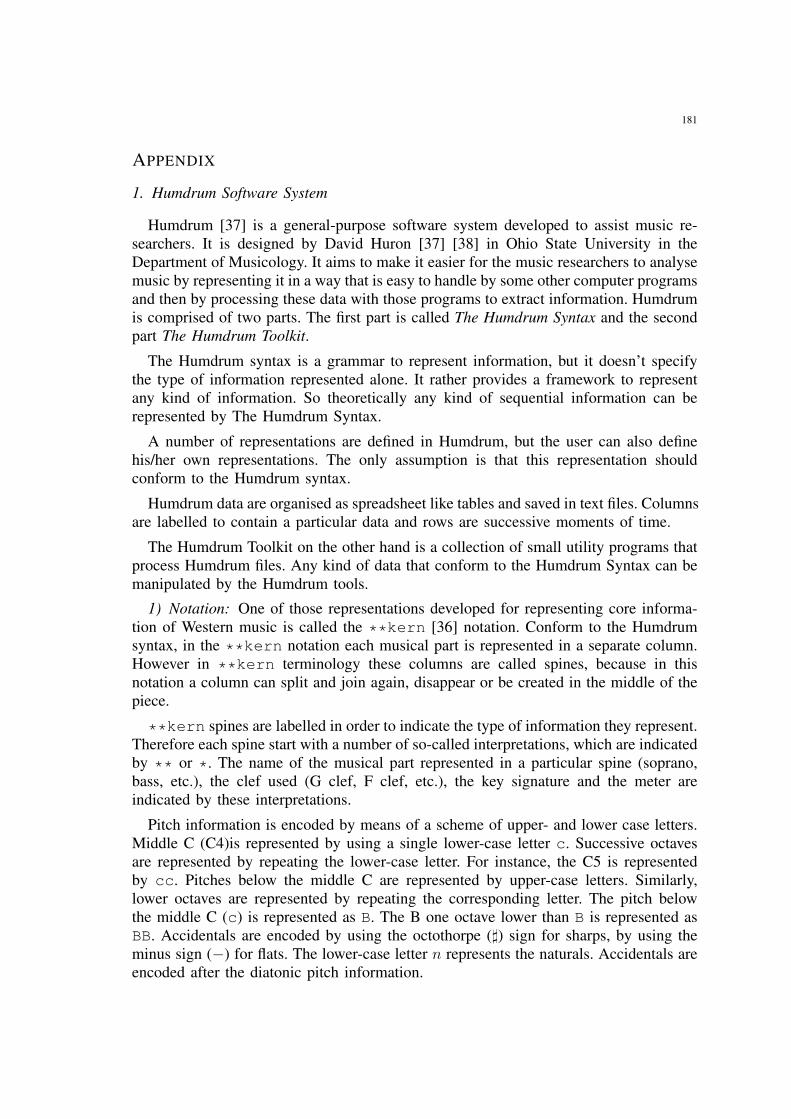
181

APPENDIX

1. Humdrum Software System

Humdrum [37] is a general-purpose software system developed to assist music re-searchers. It is designed by David Huron [37] [38] in Ohio State University in theDepartment of Musicology. It aims to make it easier for the music researchers to analysemusic by representing it in a way that is easy to handle by some other computer programsand then by processing these data with those programs to extract information. Humdrumis comprised of two parts. The first part is called The Humdrum Syntax and the secondpart The Humdrum Toolkit.

The Humdrum syntax is a grammar to represent information, but it doesn’t specifythe type of information represented alone. It rather provides a framework to representany kind of information. So theoretically any kind of sequential information can berepresented by The Humdrum Syntax.

A number of representations are defined in Humdrum, but the user can also definehis/her own representations. The only assumption is that this representation shouldconform to the Humdrum syntax.

Humdrum data are organised as spreadsheet like tables and saved in text files. Columnsare labelled to contain a particular data and rows are successive moments of time.

The Humdrum Toolkit on the other hand is a collection of small utility programs thatprocess Humdrum files. Any kind of data that conform to the Humdrum Syntax can bemanipulated by the Humdrum tools.

1) Notation: One of those representations developed for representing core informa-tion of Western music is called the **kern [36] notation. Conform to the Humdrumsyntax, in the **kern notation each musical part is represented in a separate column.However in **kern terminology these columns are called spines, because in thisnotation a column can split and join again, disappear or be created in the middle of thepiece.

**kern spines are labelled in order to indicate the type of information they represent.Therefore each spine start with a number of so-called interpretations, which are indicatedby ** or *. The name of the musical part represented in a particular spine (soprano,bass, etc.), the clef used (G clef, F clef, etc.), the key signature and the meter areindicated by these interpretations.

Pitch information is encoded by means of a scheme of upper- and lower case letters.Middle C (C4)is represented by using a single lower-case letter c. Successive octavesare represented by repeating the lower-case letter. For instance, the C5 is representedby cc. Pitches below the middle C are represented by upper-case letters. Similarly,lower octaves are represented by repeating the corresponding letter. The pitch belowthe middle C (c) is represented as B. The B one octave lower than B is represented asBB. Accidentals are encoded by using the octothorpe (]) sign for sharps, by using theminus sign (−) for flats. The lower-case letter n represents the naturals. Accidentals areencoded after the diatonic pitch information.

182

The durations of the corresponding notes are represented by reciprocal numbers: 1for the whole note, 2 for the half note, 4 for the quarter note, etc.

Fig. 85. A six notes long melody from the Inventio 01 is shown.

Ornaments, slurs, ties, phrases, measures and many other musical concepts can beencoded by using the **kern notation. However, in this thesis, I disregarded them.The melody shown in Figure 85 is encoded in **kern as follows:

**kern

*staff1

*clefG2

*k[]

*M4/416c16d16e16f16d16e16c

*-

2. Open Music

Open Music is a visual programming environment to support computer aided com-position under Macintosh. It is developed by IRCAM Centre Pompidou [39].

It is based on the programming language LISP or more precisely on the objectoriented extension of LISP, which is called CLOS (Common LISP Object System).Open Music implements plenty of objects that can basically be dragged and dropped tothe programming environment and connected together to create a program. These smallprograms can then be saved into patches and patches can then be connected to createbigger programs.

Documents

A Paradigmatic Approach for the Melodic Analysis · A Paradigmatic Approach for the Melodic Analysis vorgelegt von Computer Engineer (MSc.) Kamil Adiloglu˘ aus Istanbul, Turkei¨