A Parameter Sweep Experiment on Topographic Effects on the

Journal of the Meteorological Society of Japan, Vol. 82, No. 3, pp. 879--893, 2004 879

A Parameter Sweep Experiment on Topographic Effects on the

Annular Variability

Seiya NISHIZAWA and Shigeo YODEN

Department of Geophysics, Kyoto University, Kyoto, Japan

(Manuscript received 29 January 2003, in final form 16 February 2004)

Abstract

Effects of surface topography on annular variability of the extratropical troposphere are examined byparameter sweep experiments with a simplified global circulation model. Amplitude of the sinusoidalsurface topography hm of zonal wavenumber m is swept as an experimental parameter in two series ofexperiments; a single zonal wavenumber, two ðm ¼ 2Þ or one ðm ¼ 1Þ, is assumed in the series of WN2 orWN1, respectively. In additional series of WN2-1, the ratio of superposition of these two components isswept as an experimental parameter. In each run, long time integrations for 4300 days are done under aperpetual winter condition.

Characteristics of the leading mode of empirical orthogonal function (EOF) of the zonal-mean zonalwind, and the surface pressure ðPsÞ, depend on the amplitude and zonal wavenumber of the surface to-pography. In the WN2 experiment, characteristics of EOF1 of zonal-mean zonal wind and Ps changedramatically around h2 ¼ 450 m, and the annular variability is divided into two types for large andsmall h2. In the WN1 experiment, on the other hand, characteristics of the annular variability do notshow such drastic changes as those in the WN2 experiment, and EOF1 of Ps shows annular pattern forall h1 from 0 m to 1000 m.

Three typical cases are analyzed in detail; h2 ¼ 0 m (FLAT), h2 ¼ 1000 m (HWN2), and h1 ¼ 1000 m(HWN1). In the HWN2 experiment, the number of the storm tracks is two, and correlation map with theindex that represents the oscillatory variability at that region shows a pattern localized in longitudesaround the region with high teleconnectivity, even though EOF1 of Ps shows annular pattern.

On the other hand, the annular variability has a sound physical basis in the FLAT and HWN1 ex-periments. Importance of the number and spatial structure of storm tracks which exist at the exits of jetstreams is also confirmed in the WN2-1 experiment.

1. Introduction

Thompson and Wallace (1998, 2000) andThompson et al. (2000) pointed out that theleading mode of low-frequency variability of theextratropical circulation is characterized by‘‘annular’’ structure in both of the Northern andSouthern Hemispheres (hereafter NH and SH,respectively), so called ‘‘annular mode’’. Theannular mode has almost zonally symmetric,

and equivalent barotropic structure from thesurface to the lower stratosphere. Yamazakiand Shinya (1999) showed that the annularmode is an internal mode of the atmosphere bya general circulation model (GCM) experimentwith fixed external forcing parameters. The an-nular mode is associated with coupling betweenthe zonal-mean zonal flow and eddies (Limpa-suvan and Hartmann 2000; Hartmann et al.2000; Kimoto et al. 2001). Baroclinic distur-bances are most important in the SH, whileplanetary waves are also important in the NH.

The SH annular mode is basically the samephenomenon as the ‘‘zonal flow vacillation’’,which is caused by the interaction between the

Corresponding author: Seiya Nishizawa, Depart-ment of Geophysics, Kyoto University, Kyoto 606-8502, Japan.E-mail: [email protected]( 2004, Meteorological Society of Japan

(V7 14/6/04 14:48) Ga/J J-1095 J. Meteor 82:3 PMU: WSL 21/05/04 AC1: WSL 28/05/04 NewCenturySchlbk) (0).3.04.05 pp. 879-893 004_P (p. 879)

zonal-mean zonal wind and baroclinic distur-bances (e.g., Yoden et al. 1987; Hartmann1995). In the NH, on the other hand, the tem-poral coherence between the Atlantic and Pa-cific mid-latitudes is weak, though the leadingmode of empirical orthogonal function (EOF)of the sea-level pressure shows an annularpattern with the same sign in these regions(Deser 2000). In the EOF analysis, some un-correlated variations may result in coherentstructure in the leading mode (Ambaum et al.2001; Itoh 2002). Ambaum et al. (2001) notedthat the North Atlantic Oscillation (NAO), andthe Pacific/North American (PNA) teleconnec-tion patterns can be identified in a physicallyconsistent way in the EOF analyses appliedto various fields, but no such identification isfound for the NH annular mode. The NH an-nular mode is not still understood physically,and relationship or independency between theNH and the SH annular modes is not clear.

Differences of the atmospheric low-frequencyvariability between the two hemispheres main-ly result from the difference of the surfaceconditions, such as the topography and theland-sea thermal contrast. Taguchi and Yoden(2002) performed a parameter sweep experi-ment on the annular variability with an ideal-ized global circulation model, in which only asinusoidal surface topography of zonal wave-number one was introduced, by changing itsamplitude as an experimental parameter. Theyshowed that the vertical linkage between thetroposphere and the stratosphere in the an-nular variability depends on the amplitude ofzonally asymmetric topography. However, theyused only one horizontal pattern of the surfacetopography, though the real topography has notonly zonal wavenumber one component, butalso higher wavenumbers.

In this study, we further examine the effectsof zonal asymmetry of the surface topographyon the annular variability, by using a similarglobal circulation model with an idealized to-pography. First, two series of parameter sweepexperiments are done with sinusoidal topogra-phy of zonal wavenumber two or one by chang-ing its amplitude as the experimental param-eter, in order to examine the dependence ofannular variability on the amplitude of to-pography. Three typical cases of a flat surface,wavenumber one topography and wavenumber

two are analyzed to examine difference in theannular variability from some viewpoints; sub-tropical westerly jet stream, storm track, tele-connectivity and so on. In addition, anotherseries of parameter sweep experiment is donewith superposed topography of zonal wave-number one and two to clarify the relationshipbetween the annular variability and stormtrack activity.

2. Model and experiment

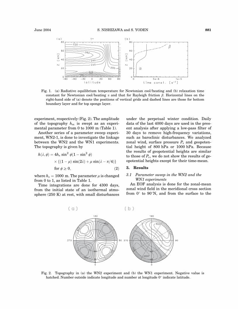
The model used in this study is basically thesame as the models used in Akahori and Yoden(1997) and Taguchi et al. (2001). The model is asimplified three-dimensional global primitive-equation model (Swamp Project 1998). A spec-tral-transform method is used for the horizon-tal advections, with a triangular truncation ofthe total wavenumber 42, and 30 s-levels areadopted in the vertical discretization (Fig. 1a,right-hand side).

Some physical processes are simplified. Ra-diative processes are represented by a simpleNewtonian heat/cooling scheme. The equilib-rium temperature is assumed to be a wintercondition in the NH, as shown in Fig. 1(a). Therelaxation time-constant a is shown in Fig. 1(b);a�1 is 20 days in the troposphere except forthe bottom two layers (5.5 and 12 days, respec-tively; Hoskins and Valdes 1990), while 4 daysin the mesosphere. Rayleigh friction is usedin the bottom boundary layer and the topsponge layer with the relaxation time-constantb shown in Fig. 1(b). All moist processes areremoved for the model, and the dry convectiveadjustment scheme is retained. Internal hori-zontal dissipation in the ‘4 form is appliedto temperature, vorticity and divergence fieldswith a damping time of 6 hours for the maxi-mum wavenumber, 42.

In the first two series of the experiments,sinusoidal surface topography is assumed onlyin the NH in the form of

hðl; fÞ

¼ 4hm sin2 fð1 � sin2 fÞ sin ml� ð2�mÞp4

n ofor fb 0;

0 for f < 0;

(

ð1Þ

where m is the zonal wavenumber, l thelongitude, and f the latitude. The zonal wave-number two or one is used in the WN2 or WN1

Journal of the Meteorological Society of Japan880 Vol. 82, No. 3


experiment, respectively (Fig. 2). The amplitudeof the topography hm is swept as an experi-mental parameter from 0 to 1000 m (Table 1).

Another series of a parameter sweep experi-ment, WN2-1, is done to investigate the linkagebetween the WN2 and the WN1 experiments.The topography is given by

hðl; fÞ ¼ 4hs sin2 fð1 � sin2 fÞ

� fð1 � mÞ sinð2lÞ þ m sinðl� p=4Þg

for fb 0; ð2Þ

where hs ¼ 1000 m. The parameter m is changedfrom 0 to 1, as listed in Table 1.

Time integrations are done for 4300 days,from the initial state of an isothermal atmo-sphere (250 K) at rest, with small disturbances

under the perpetual winter condition. Dailydata of the last 4000 days are used in the pres-ent analysis after applying a low-pass filter of30 days to remove high-frequency variations,such as baroclinic disturbances. We analyzedzonal wind, surface pressure Ps and geopoten-tial height of 800 hPa or 1000 hPa. Becausethe results of geopotential heights are similarto those of Ps, we do not show the results of ge-opotential heights except for their time-mean.

3. Results

3.1 Parameter sweep in the WN2 and theWN1 experiments

An EOF analysis is done for the zonal-meanzonal wind field in the meridional cross sectionfrom 0� to 90�N, and from the surface to the

Fig. 1. (a) Radiative equilibrium temperature for Newtonian cool/heating and (b) relaxation timeconstant for Newtonian cool/heating a and that for Rayleigh friction b. Horizontal lines on theright-hand side of (a) denote the positions of vertical grids and dashed lines are those for bottomboundary layer and for top sponge layer.

Fig. 2. Topography in (a) the WN2 experiment and (b) the WN1 experiment. Negative value ishatched. Number outside indicate longitude and number at longitude 0� indicate latitude.

S. NISHIZAWA and S. YODEN 881June 2004


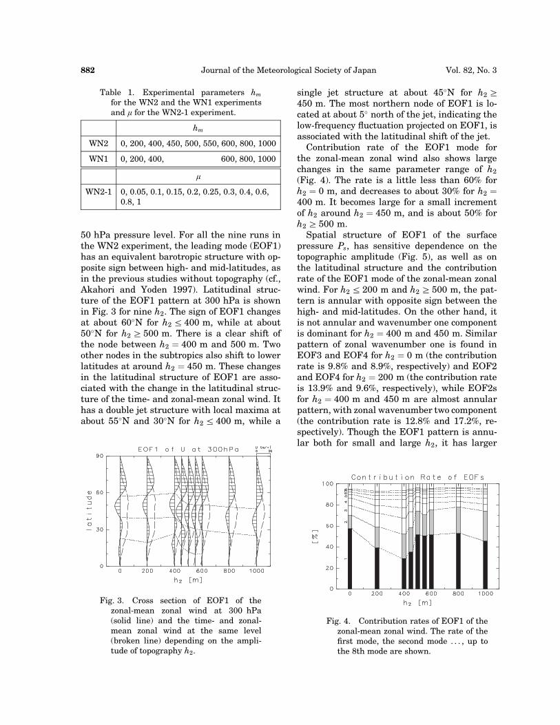
50 hPa pressure level. For all the nine runs inthe WN2 experiment, the leading mode (EOF1)has an equivalent barotropic structure with op-posite sign between high- and mid-latitudes, asin the previous studies without topography (cf.,Akahori and Yoden 1997). Latitudinal struc-ture of the EOF1 pattern at 300 hPa is shownin Fig. 3 for nine h2. The sign of EOF1 changesat about 60�N for h2 a 400 m, while at about50�N for h2 b 500 m. There is a clear shift ofthe node between h2 ¼ 400 m and 500 m. Twoother nodes in the subtropics also shift to lowerlatitudes at around h2 ¼ 450 m. These changesin the latitudinal structure of EOF1 are asso-ciated with the change in the latitudinal struc-ture of the time- and zonal-mean zonal wind. Ithas a double jet structure with local maxima atabout 55�N and 30�N for h2 a 400 m, while a

single jet structure at about 45�N for h2 b

450 m. The most northern node of EOF1 is lo-cated at about 5� north of the jet, indicating thelow-frequency fluctuation projected on EOF1, isassociated with the latitudinal shift of the jet.

Contribution rate of the EOF1 mode forthe zonal-mean zonal wind also shows largechanges in the same parameter range of h2

(Fig. 4). The rate is a little less than 60% forh2 ¼ 0 m, and decreases to about 30% for h2 ¼400 m. It becomes large for a small incrementof h2 around h2 ¼ 450 m, and is about 50% forh2 b 500 m.

Spatial structure of EOF1 of the surfacepressure Ps, has sensitive dependence on thetopographic amplitude (Fig. 5), as well as onthe latitudinal structure and the contributionrate of the EOF1 mode of the zonal-mean zonalwind. For h2 a 200 m and h2 b 500 m, the pat-tern is annular with opposite sign between thehigh- and mid-latitudes. On the other hand, itis not annular and wavenumber one componentis dominant for h2 ¼ 400 m and 450 m. Similarpattern of zonal wavenumber one is found inEOF3 and EOF4 for h2 ¼ 0 m (the contributionrate is 9.8% and 8.9%, respectively) and EOF2and EOF4 for h2 ¼ 200 m (the contribution rateis 13.9% and 9.6%, respectively), while EOF2sfor h2 ¼ 400 m and 450 m are almost annularpattern, with zonal wavenumber two component(the contribution rate is 12.8% and 17.2%, re-spectively). Though the EOF1 pattern is annu-lar both for small and large h2, it has larger

Table 1. Experimental parameters hm

for the WN2 and the WN1 experimentsand m for the WN2-1 experiment.

hm

WN2 0, 200, 400, 450, 500, 550, 600, 800, 1000

WN1 0, 200, 400, 600, 800, 1000

m

WN2-1 0, 0.05, 0.1, 0.15, 0.2, 0.25, 0.3, 0.4, 0.6,0.8, 1

Fig. 3. Cross section of EOF1 of thezonal-mean zonal wind at 300 hPa(solid line) and the time- and zonal-mean zonal wind at the same level(broken line) depending on the ampli-tude of topography h2.

Fig. 4. Contribution rates of EOF1 of thezonal-mean zonal wind. The rate of thefirst mode, the second mode . . . , up tothe 8th mode are shown.



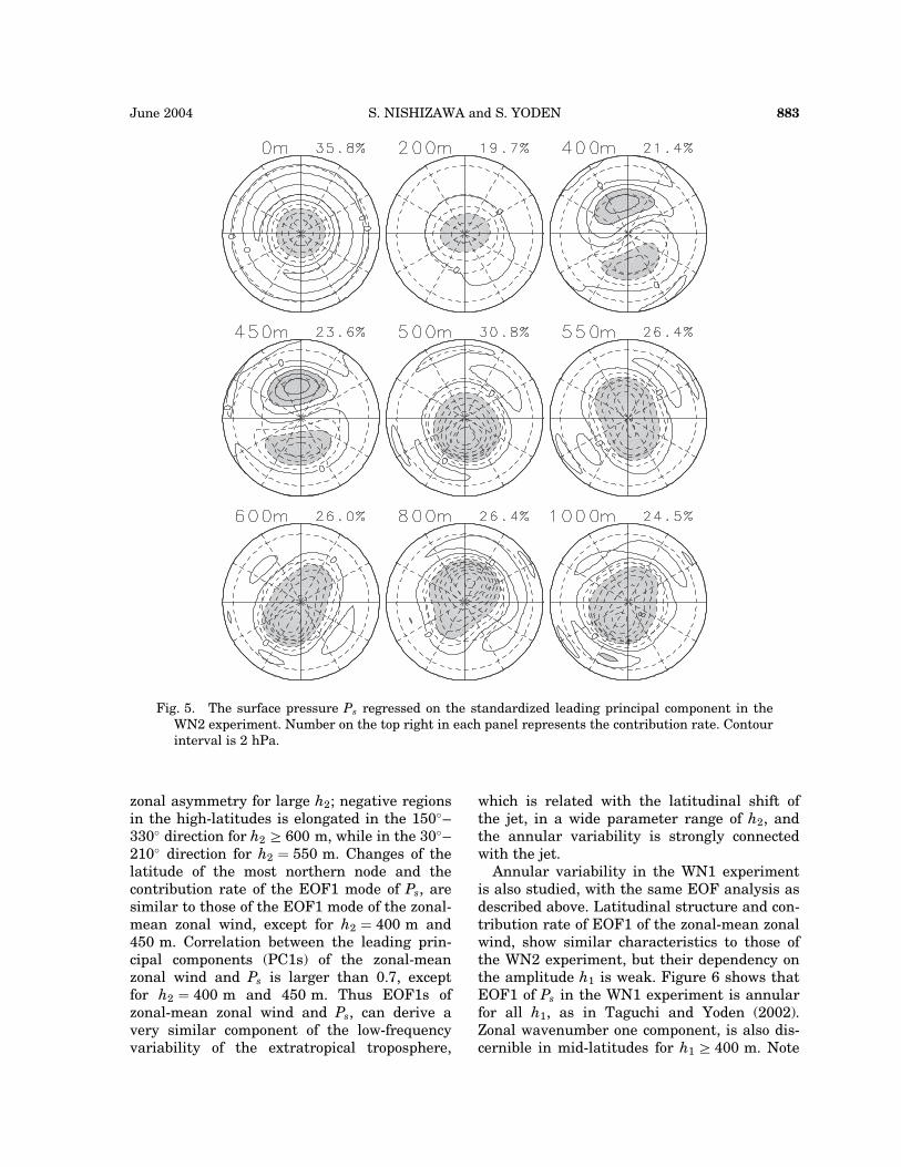
zonal asymmetry for large h2; negative regionsin the high-latitudes is elongated in the 150�–330� direction for h2 b 600 m, while in the 30�–210� direction for h2 ¼ 550 m. Changes of thelatitude of the most northern node and thecontribution rate of the EOF1 mode of Ps, aresimilar to those of the EOF1 mode of the zonal-mean zonal wind, except for h2 ¼ 400 m and450 m. Correlation between the leading prin-cipal components (PC1s) of the zonal-meanzonal wind and Ps is larger than 0.7, exceptfor h2 ¼ 400 m and 450 m. Thus EOF1s ofzonal-mean zonal wind and Ps, can derive avery similar component of the low-frequencyvariability of the extratropical troposphere,

which is related with the latitudinal shift ofthe jet, in a wide parameter range of h2, andthe annular variability is strongly connectedwith the jet.

Annular variability in the WN1 experimentis also studied, with the same EOF analysis asdescribed above. Latitudinal structure and con-tribution rate of EOF1 of the zonal-mean zonalwind, show similar characteristics to those ofthe WN2 experiment, but their dependency onthe amplitude h1 is weak. Figure 6 shows thatEOF1 of Ps in the WN1 experiment is annularfor all h1, as in Taguchi and Yoden (2002).Zonal wavenumber one component, is also dis-cernible in mid-latitudes for h1 b 400 m. Note

Fig. 5. The surface pressure Ps regressed on the standardized leading principal component in theWN2 experiment. Number on the top right in each panel represents the contribution rate. Contourinterval is 2 hPa.



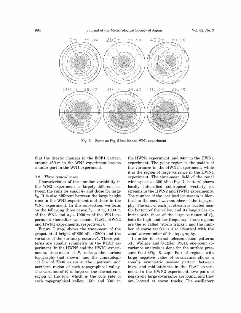
that the drastic changes in the EOF1 patternaround 450 m in the WN2 experiment has nocounter part in the WN1 experiment.

3.2 Three typical casesCharacteristics of the annular variability in

the WN2 experiment is largely different be-tween the runs for small h2 and those for largeh2. It is also different between the large heightruns in the WN2 experiment and those in theWN1 experiment. In this subsection, we focuson the following three cases; h2 ¼ 0 m, 1000 mof the WN2 and h1 ¼ 1000 m of the WN1 ex-periment (hereafter we denote FLAT, HWN2and HWN1 experiments, respectively).

Figure 7 (top) shows the time-mean of thegeopotential height of 800 hPa (Z800) and thevariance of the surface pressure Ps. These pat-terns are zonally symmetric in the FLAT ex-periment. In the HWN2 and the HWN1 experi-ments, time-mean of Ps reflects the surfacetopography (not shown), and the climatologi-cal low of Z800 exists at the upstream andnorthern region of each topographical valley.The variance of Ps is large on the downstreamregion of the low, which is the pole side ofeach topographical valley; 150� and 330� in

the HWN2 experiment, and 345� in the HWN1experiment. The polar region is the saddle ofthe variance in the HWN2 experiment, whileit is the region of large variance in the HWN1experiment. The time-mean field of the zonalwind speed at 300 hPa (Fig. 7, bottom) showslocally intensified subtropical westerly jetstreams in the HWN2 and HWN1 experiments.The number of the localized jet stream is iden-tical to the zonal wavenumber of the topogra-phy. The exit of each jet stream is located nearthe bottom of the valley, and its longitudes co-incide with those of the large variance of Ps,both for high- and low-frequency. These regionsare the so called ‘‘storm tracks’’, and the num-ber of storm tracks is also identical with thezonal wavenumber of the topography.

In order to extract teleconnection patterns(cf., Wallace and Gutzler 1981), one-point co-variance analysis is done for the surface pres-sure field (Fig. 8, top). Pair of regions withlarge negative value of covariance, shows azonally symmetric seesaw pattern betweenhigh- and mid-latitudes in the FLAT experi-ment. In the HWN2 experiment, two pairs ofnegatively large covariance are found, and theyare located at storm tracks. The oscillatory

Fig. 6. Same as Fig. 5 but for the WN1 experiment.



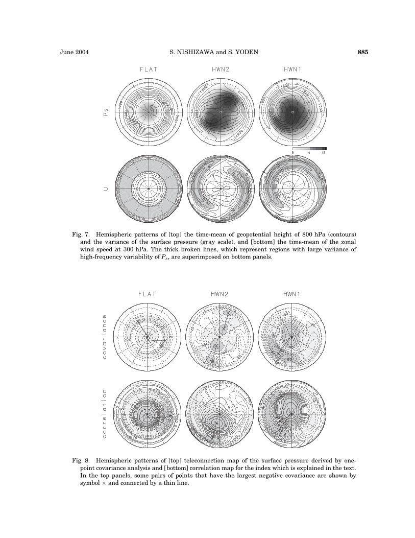
Fig. 7. Hemispheric patterns of [top] the time-mean of geopotential height of 800 hPa (contours)and the variance of the surface pressure (gray scale), and [bottom] the time-mean of the zonalwind speed at 300 hPa. The thick broken lines, which represent regions with large variance ofhigh-frequency variability of Ps, are superimposed on bottom panels.

Fig. 8. Hemispheric patterns of [top] teleconnection map of the surface pressure derived by one-point covariance analysis and [bottom] correlation map for the index which is explained in the text.In the top panels, some pairs of points that have the largest negative covariance are shown bysymbol � and connected by a thin line.



variabilities with large teleconnectivity are lo-calized in longitudes. In the HWN1 experiment,on the other hand, only one pair is found, andits north-side region is in the polar region, andthe opposite south-side region, centered at 320�,extends in longitudes widely.

After introducing an index which is the dif-ference of normalized Ps with its standard de-viation at the two points with the largest nega-tive covariance, a correlation map of Ps withthe index is made (Fig. 8 bottom). In the FLATand the HWN1 experiments, the correlationpattern is annular and similar to the EOF1pattern of Ps shown in Fig. 6. The region withhigh correlation is zonally elongated in mid-latitudes. Pattern correlations between thecorrelation pattern, and the EOF pattern ina sector (l0 þ 90� a la l0 þ 270�, fb 30�N; l:longitude, l0: longitude of the southern point ofthe pair, f: latitude), are �0:43 and �0:54 inthe FLAT and the HWN1 experiments, respec-tively, and the correlation coefficient betweenPC1 of Ps and the index is �0:87 and �0:95,respectively.

In the HWN2 experiment, on the other hand,large value of the correlation is rather limitednear the points to define the index. Correla-tion around 160� in mid-latitudes is near to 0,where EOF1 of Ps has a non-zero value with thesame sign as that around 340� in mid-latitudes.The correlation pattern is zonally asymmetric,and not similar to the EOF1 pattern. Patterncorrelation in the sector is �0:33, and correla-tion between the index1, that is calculatedfrom the pair at about 340� and the PC1 of Ps

is �0:77, while correlation between anotherindex2, at about 160� and the PC1 is �0:57(Table 2). These absolute values of the cor-relations are not so high as those in the FLAT

or the WN1 experiment. Correlation coefficientbetween index1 and index2 is 0.07, and thisvalue has no statistical significance. Thus vari-ability at the two storm tracks is almost inde-pendent.

3.3 Parameter sweep in the WN2-1 experimentIn order to examine the relationship be-

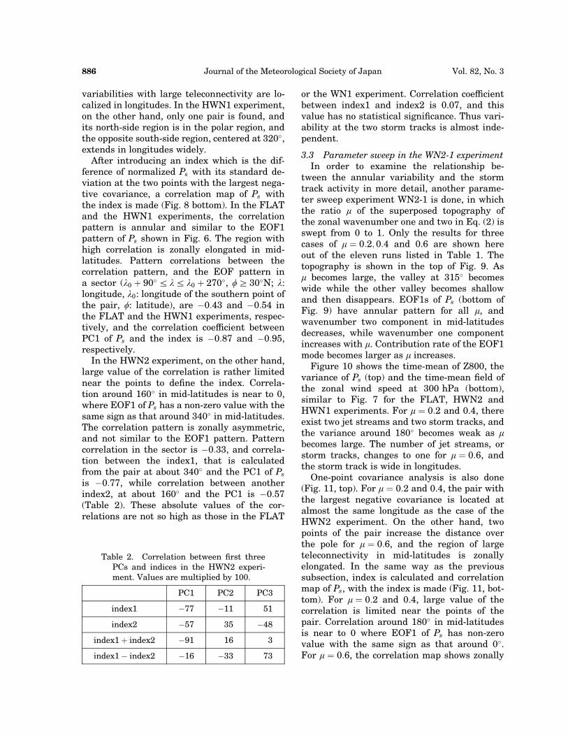
tween the annular variability and the stormtrack activity in more detail, another parame-ter sweep experiment WN2-1 is done, in whichthe ratio m of the superposed topography ofthe zonal wavenumber one and two in Eq. (2) isswept from 0 to 1. Only the results for threecases of m ¼ 0:2; 0:4 and 0.6 are shown hereout of the eleven runs listed in Table 1. Thetopography is shown in the top of Fig. 9. Asm becomes large, the valley at 315� becomeswide while the other valley becomes shallowand then disappears. EOF1s of Ps (bottom ofFig. 9) have annular pattern for all m, andwavenumber two component in mid-latitudesdecreases, while wavenumber one componentincreases with m. Contribution rate of the EOF1mode becomes larger as m increases.

Figure 10 shows the time-mean of Z800, thevariance of Ps (top) and the time-mean field ofthe zonal wind speed at 300 hPa (bottom),similar to Fig. 7 for the FLAT, HWN2 andHWN1 experiments. For m ¼ 0:2 and 0.4, thereexist two jet streams and two storm tracks, andthe variance around 180� becomes weak as m

becomes large. The number of jet streams, orstorm tracks, changes to one for m ¼ 0:6, andthe storm track is wide in longitudes.

One-point covariance analysis is also done(Fig. 11, top). For m ¼ 0:2 and 0.4, the pair withthe largest negative covariance is located atalmost the same longitude as the case of theHWN2 experiment. On the other hand, twopoints of the pair increase the distance overthe pole for m ¼ 0:6, and the region of largeteleconnectivity in mid-latitudes is zonallyelongated. In the same way as the previoussubsection, index is calculated and correlationmap of Ps, with the index is made (Fig. 11, bot-tom). For m ¼ 0:2 and 0.4, large value of thecorrelation is limited near the points of thepair. Correlation around 180� in mid-latitudesis near to 0 where EOF1 of Ps has non-zerovalue with the same sign as that around 0�.For m ¼ 0:6, the correlation map shows zonally

Table 2. Correlation between first threePCs and indices in the HWN2 experi-ment. Values are multiplied by 100.

PC1 PC2 PC3

index1 �77 �11 51

index2 �57 35 �48

index1 þ index2 �91 16 3

index1 � index2 �16 �33 73



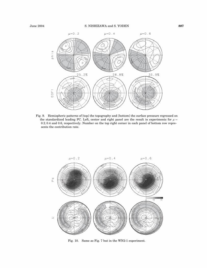
Fig. 9. Hemispheric patterns of [top] the topography and [bottom] the surface pressure regressed onthe standardized leading PC. Left, center and right panel are the result in experiments for m ¼0:2; 0:4 and 0:6, respectively. Number on the top right corner in each panel of bottom row repre-sents the contribution rate.

Fig. 10. Same as Fig. 7 but in the WN2-1 experiment.



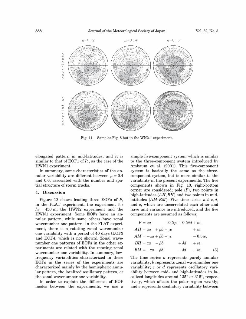
elongated pattern in mid-latitudes, and it issimilar to that of EOF1 of Ps, as the case of theHWN1 experiment.

In summary, some characteristics of the an-nular variability are different between m ¼ 0:4and 0.6, associated with the number and spa-tial structure of storm tracks.

4. Discussion

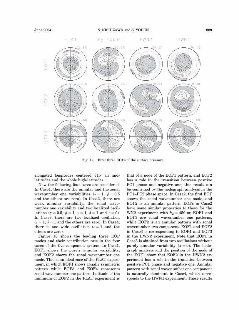
Figure 12 shows leading three EOFs of Ps

in the FLAT experiment, the experiment forh2 ¼ 450 m, the HWN2 experiment and theHWN1 experiment. Some EOFs have an an-nular pattern, while some others have zonalwavenumber one pattern. In the FLAT experi-ment, there is a rotating zonal wavenumberone variability with a period of 40 days (EOF3and EOF4, which is not shown). Zonal wave-number one patterns of EOFs in the other ex-periments are related with the rotating zonalwavenumber one variability. In summary, low-frequency variabilities characterized in theseEOFs in the series of the experiments arecharacterized mainly by the hemispheric annu-lar pattern, the localized oscillatory pattern, orthe zonal wavenumber one variability.

In order to explain the difference of EOFmodes between the experiments, we use a

simple five-component system which is similarto the three-component system introduced byAmbaum et al. (2001). This five-componentsystem is basically the same as the three-component system, but is more similar to thevariability in the present experiments. The fivecomponents shown in Fig. 13, right-bottomcorner are considered; pole ðPÞ, two points inhigh-latitudes ðAH;BHÞ and two points in mid-latitudes ðAM;BMÞ. Five time series a; b; c;d,and e, which are uncorrelated each other andhave unit variance are introduced, and the fivecomponents are assumed as follows;

P ¼ aa þ 0:5gcþ 0:5ddþ ee;

AH ¼ aa þ bbþ gc þ ee;

AM ¼ �aaþ bb� gc � 0:5ee;

BH ¼ aa � bb þ dd þ ee;

BM ¼ �aa� bb � dd � ee: ð3Þ

The time series a represents purely annularvariability; b represents zonal wavenumber onevariability; c or d represents oscillatory vari-ability between mid- and high-latitudes in lo-calized longitudes around 135� or 315�, respec-tively, which affects the polar region weakly;and e represents oscillatory variability between

Fig. 11. Same as Fig. 8 but in the WN2-1 experiment.



elongated longitudes centered 315� in mid-latitudes and the whole high-latitudes.

Now the following four cases are considered.In Case1, there are the annular and the zonalwavenumber one variabilities (a ¼ 1, b ¼ 0:5and the others are zero). In Case2, there areweak annular variability, the zonal wave-number one variability and two localized oscil-lations (a ¼ 0:5, b ¼ 1, g ¼ 1, d ¼ 1 and e ¼ 0).In Case3, there are two localized oscillation(g ¼ 1, d ¼ 1 and the others are zero). In Case4,there is one wide oscillation (e ¼ 1 and theothers are zero).

Figure 13 shows the leading three EOFmodes and their contribution rate in the fourcases of the five-component system. In Case1,EOF1 shows the purely annular variability,and EOF2 shows the zonal wavenumber onemode. This is an ideal case of the FLAT experi-ment, in which EOF1 shows zonally symmetricpattern while EOF3 and EOF4 representszonal wavenumber one pattern. Latitude of theminimum of EOF2 in the FLAT experiment is

that of a node of the EOF1 pattern, and EOF2has a role in the transition between positivePC1 phase and negative one; this result canbe confirmed by the hodograph analysis in thePC1–PC2 phase space. In Case2, the first EOFshows the zonal wavenumber one mode, andEOF2 is an annular pattern. EOFs in Case2have some similar properties to these for theWN2 experiment with h2 ¼ 450 m; EOF1 andEOF3 are zonal wavenumber one patterns,while EOF2 is an annular pattern with zonalwavenumber two component. EOF1 and EOF2in Case3 is corresponding to EOF1 and EOF3in the HWN2 experiment. Note that EOF1 inCase3 is obtained from two oscillations withoutpurely annular variability ða ¼ 0Þ. The hodo-graph analysis and the position of the node ofthe EOF1 show that EOF2 in the HWN2 ex-periment has a role in the transition betweenpositive PC1 phase and negative one. Annularpattern with zonal wavenumber one componentis naturally dominant in Case4, which corre-sponds to the HWN1 experiment. These results

Fig. 12. First three EOFs of the surface pressure.



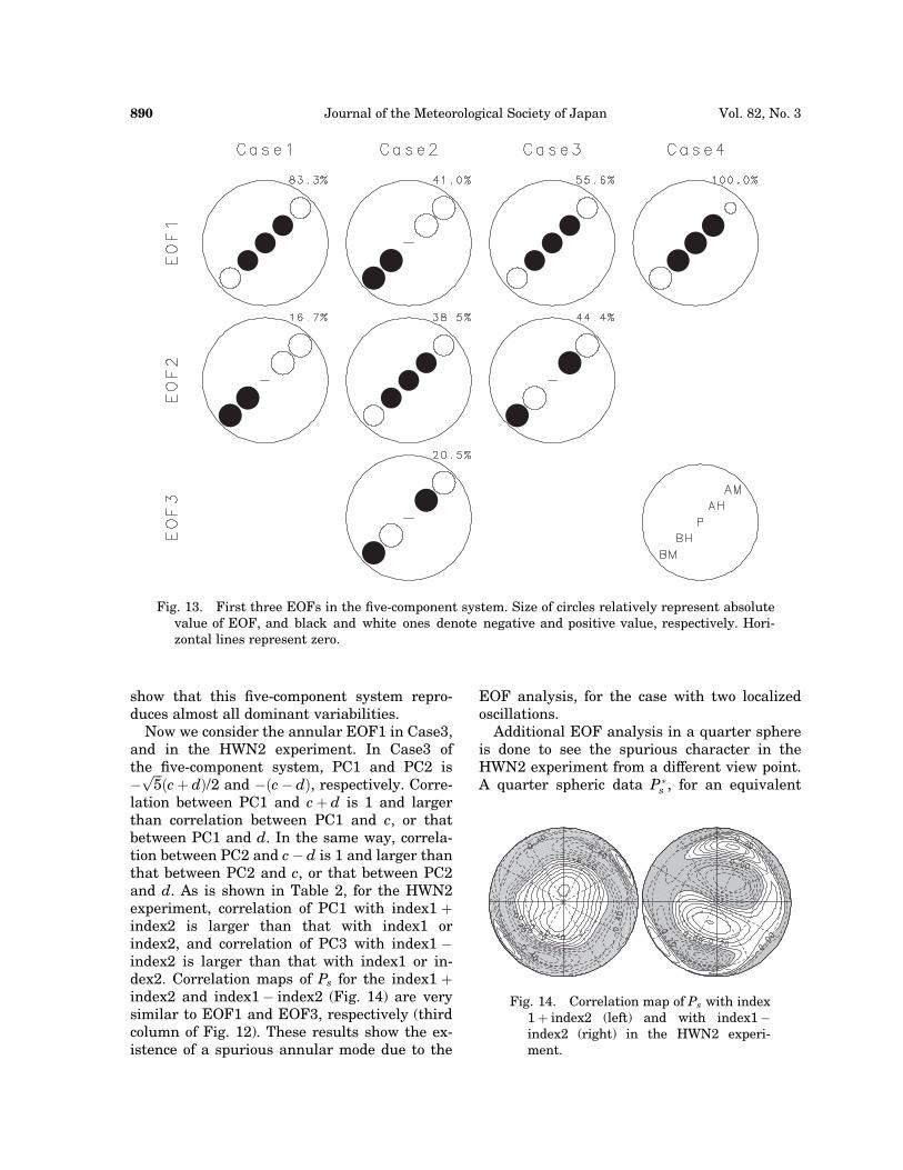
show that this five-component system repro-duces almost all dominant variabilities.

Now we consider the annular EOF1 in Case3,and in the HWN2 experiment. In Case3 ofthe five-component system, PC1 and PC2 is�

ffiffiffi5

pðcþ dÞ/2 and �ðc� dÞ, respectively. Corre-

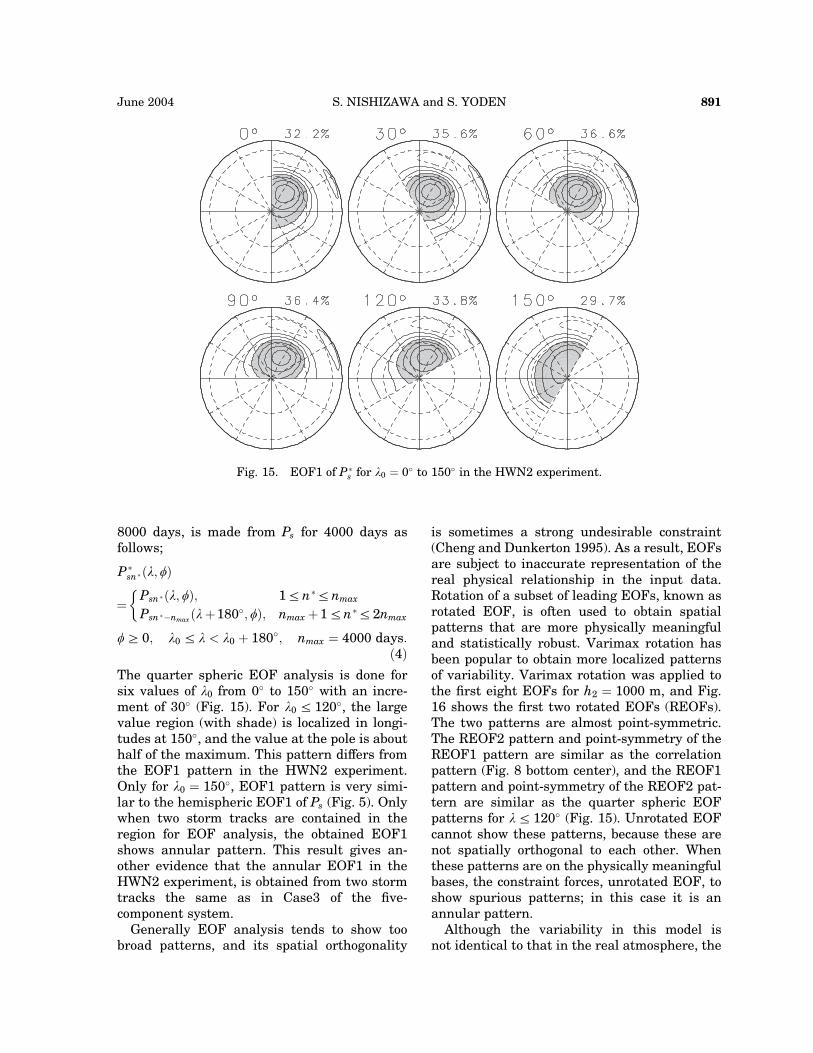
lation between PC1 and cþ d is 1 and largerthan correlation between PC1 and c, or thatbetween PC1 and d. In the same way, correla-tion between PC2 and c� d is 1 and larger thanthat between PC2 and c, or that between PC2and d. As is shown in Table 2, for the HWN2experiment, correlation of PC1 with index1 þindex2 is larger than that with index1 orindex2, and correlation of PC3 with index1 �index2 is larger than that with index1 or in-dex2. Correlation maps of Ps for the index1 þindex2 and index1 � index2 (Fig. 14) are verysimilar to EOF1 and EOF3, respectively (thirdcolumn of Fig. 12). These results show the ex-istence of a spurious annular mode due to the

EOF analysis, for the case with two localizedoscillations.

Additional EOF analysis in a quarter sphereis done to see the spurious character in theHWN2 experiment from a different view point.A quarter spheric data P�

s , for an equivalent

Fig. 13. First three EOFs in the five-component system. Size of circles relatively represent absolutevalue of EOF, and black and white ones denote negative and positive value, respectively. Hori-zontal lines represent zero.

Fig. 14. Correlation map of Ps with index1 þ index2 (left) and with index1�index2 (right) in the HWN2 experi-ment.



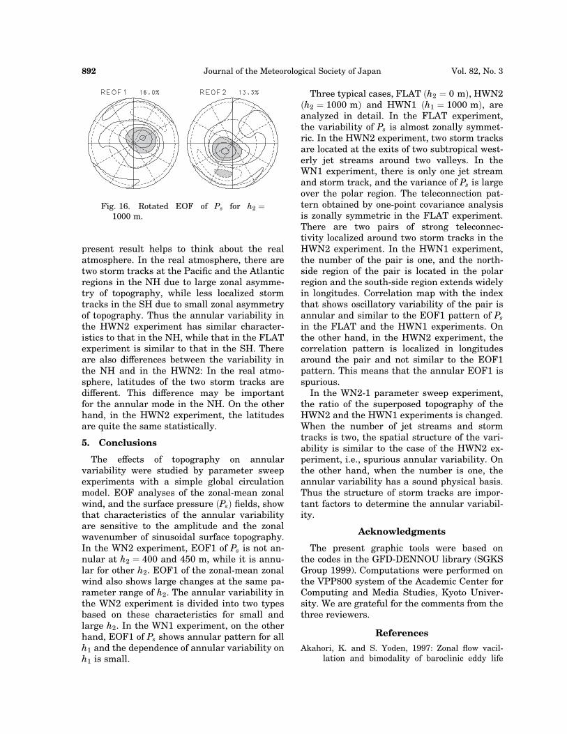
8000 days, is made from Ps for 4000 days asfollows;

P�sn� ðl; fÞ

¼ Psn � ðl; fÞ; 1an�anmax

Psn ��nmaxðlþ180�; fÞ; nmax þ1an�a2nmax

�

fb 0; l0 a l < l0 þ 180�; nmax ¼ 4000 days:ð4Þ

The quarter spheric EOF analysis is done forsix values of l0 from 0� to 150� with an incre-ment of 30� (Fig. 15). For l0 a 120�, the largevalue region (with shade) is localized in longi-tudes at 150�, and the value at the pole is abouthalf of the maximum. This pattern differs fromthe EOF1 pattern in the HWN2 experiment.Only for l0 ¼ 150�, EOF1 pattern is very simi-lar to the hemispheric EOF1 of Ps (Fig. 5). Onlywhen two storm tracks are contained in theregion for EOF analysis, the obtained EOF1shows annular pattern. This result gives an-other evidence that the annular EOF1 in theHWN2 experiment, is obtained from two stormtracks the same as in Case3 of the five-component system.

Generally EOF analysis tends to show toobroad patterns, and its spatial orthogonality

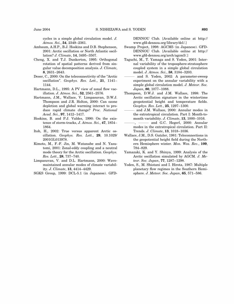
is sometimes a strong undesirable constraint(Cheng and Dunkerton 1995). As a result, EOFsare subject to inaccurate representation of thereal physical relationship in the input data.Rotation of a subset of leading EOFs, known asrotated EOF, is often used to obtain spatialpatterns that are more physically meaningfuland statistically robust. Varimax rotation hasbeen popular to obtain more localized patternsof variability. Varimax rotation was applied tothe first eight EOFs for h2 ¼ 1000 m, and Fig.16 shows the first two rotated EOFs (REOFs).The two patterns are almost point-symmetric.The REOF2 pattern and point-symmetry of theREOF1 pattern are similar as the correlationpattern (Fig. 8 bottom center), and the REOF1pattern and point-symmetry of the REOF2 pat-tern are similar as the quarter spheric EOFpatterns for la 120� (Fig. 15). Unrotated EOFcannot show these patterns, because these arenot spatially orthogonal to each other. Whenthese patterns are on the physically meaningfulbases, the constraint forces, unrotated EOF, toshow spurious patterns; in this case it is anannular pattern.

Although the variability in this model isnot identical to that in the real atmosphere, the

Fig. 15. EOF1 of P�s for l0 ¼ 0� to 150� in the HWN2 experiment.



present result helps to think about the realatmosphere. In the real atmosphere, there aretwo storm tracks at the Pacific and the Atlanticregions in the NH due to large zonal asymme-try of topography, while less localized stormtracks in the SH due to small zonal asymmetryof topography. Thus the annular variability inthe HWN2 experiment has similar character-istics to that in the NH, while that in the FLATexperiment is similar to that in the SH. Thereare also differences between the variability inthe NH and in the HWN2: In the real atmo-sphere, latitudes of the two storm tracks aredifferent. This difference may be importantfor the annular mode in the NH. On the otherhand, in the HWN2 experiment, the latitudesare quite the same statistically.

5. Conclusions

The effects of topography on annularvariability were studied by parameter sweepexperiments with a simple global circulationmodel. EOF analyses of the zonal-mean zonalwind, and the surface pressure ðPsÞ fields, showthat characteristics of the annular variabilityare sensitive to the amplitude and the zonalwavenumber of sinusoidal surface topography.In the WN2 experiment, EOF1 of Ps is not an-nular at h2 ¼ 400 and 450 m, while it is annu-lar for other h2. EOF1 of the zonal-mean zonalwind also shows large changes at the same pa-rameter range of h2. The annular variability inthe WN2 experiment is divided into two typesbased on these characteristics for small andlarge h2. In the WN1 experiment, on the otherhand, EOF1 of Ps shows annular pattern for allh1 and the dependence of annular variability onh1 is small.

Three typical cases, FLAT ðh2 ¼ 0 mÞ, HWN2ðh2 ¼ 1000 mÞ and HWN1 ðh1 ¼ 1000 mÞ, areanalyzed in detail. In the FLAT experiment,the variability of Ps is almost zonally symmet-ric. In the HWN2 experiment, two storm tracksare located at the exits of two subtropical west-erly jet streams around two valleys. In theWN1 experiment, there is only one jet streamand storm track, and the variance of Ps is largeover the polar region. The teleconnection pat-tern obtained by one-point covariance analysisis zonally symmetric in the FLAT experiment.There are two pairs of strong teleconnec-tivity localized around two storm tracks in theHWN2 experiment. In the HWN1 experiment,the number of the pair is one, and the north-side region of the pair is located in the polarregion and the south-side region extends widelyin longitudes. Correlation map with the indexthat shows oscillatory variability of the pair isannular and similar to the EOF1 pattern of Ps

in the FLAT and the HWN1 experiments. Onthe other hand, in the HWN2 experiment, thecorrelation pattern is localized in longitudesaround the pair and not similar to the EOF1pattern. This means that the annular EOF1 isspurious.

In the WN2-1 parameter sweep experiment,the ratio of the superposed topography of theHWN2 and the HWN1 experiments is changed.When the number of jet streams and stormtracks is two, the spatial structure of the vari-ability is similar to the case of the HWN2 ex-periment, i.e., spurious annular variability. Onthe other hand, when the number is one, theannular variability has a sound physical basis.Thus the structure of storm tracks are impor-tant factors to determine the annular variabil-ity.

Acknowledgments

The present graphic tools were based onthe codes in the GFD-DENNOU library (SGKSGroup 1999). Computations were performed onthe VPP800 system of the Academic Center forComputing and Media Studies, Kyoto Univer-sity. We are grateful for the comments from thethree reviewers.

References

Akahori, K. and S. Yoden, 1997: Zonal flow vacil-lation and bimodality of baroclinic eddy life

Fig. 16. Rotated EOF of Ps for h2 ¼1000 m.



cycles in a simple global circulation model. J.Atmos. Sci., 54, 2349–2361.

Ambaum, A.H.P., B.J. Hoskins and D.B. Stephenson,2001: Arctic oscillation or North Atlantic oscil-lation? J. Climate, 14, 3495–3507.

Cheng, X. and T.J. Dunkerton, 1995: Orthogonalrotation of spatial patterns derived from sin-gular value decomposition analysis. J. Climate,8, 2631–2643.

Deser, C., 2000: On the teleconnectivity of the ‘‘Arcticoscillation’’. Geophys. Res. Lett., 21, 1141–1144.

Hartmann, D.L., 1995: A PV view of zonal flow vac-illation. J. Atmos. Sci., 52, 2561–2576.

Hartmann, J.M., Wallace, V. Limpasuvan, D.W.J.Thompson and J.R. Holton, 2000: Can ozonedepletion and global warming interact to pro-duce rapid climate change? Proc. NationalAcad. Sci., 97, 1412–1417.

Hoskins, B. and P.J. Valdes, 1990: On the exis-tence of storm-tracks, J. Atmos. Sci., 47, 1854–1864.

Itoh, H., 2002: True versus apparent Arctic os-cillation. Geophys. Res. Lett., 29, 10.1029/2001GL013978.

Kimoto, M., F.-F. Jin, M. Watanabe and N. Yasu-tomi, 2001: Zonal-eddy coupling and a neutralmode theory for the Arctic oscillation. Geophys.Res. Lett., 28, 737–740.

Limpasuvan, V. and D.L. Hartmann, 2000: Wave-maintained annular modes of climate variabil-ity. J. Climate, 13, 4414–4429.

SGKS Group, 1999: DCL-5.1 (in Japanese). GFD-

DENNOU Club. [Available online at http://www.gfd-dennou.org/library/dcl/.]

Swamp Project, 1998: AGCM5 (in Japanese). GFD-DENNOU Club. [Available online at http://www.gfd-dennou.org/arch/agcm5/.]

Taguchi, M., T. Yamaga and S. Yoden, 2001: Inter-nal variability of the troposphere-stratospherecoupled system in a simple global circulationmodel. J. Atmos. Sci., 58, 3184–3203.

——— and S. Yoden, 2002: A parameter-sweepexperiment on the annular variability with asimple global circulation model. J. Meteor. Soc.Japan, 80, 1077–1088.

Thompson, D.W.J. and J.M. Wallace, 1998: TheArctic oscillation signature in the wintertimegeopotential height and temperature fields.Geophys. Res. Lett., 25, 1297–1300.

——— and J.M. Wallace, 2000: Annular modes inthe extratropical circulation. Part I: Month-to-month variability. J. Climate, 13, 1000–1016.

———, ——— and G.C. Hegerl, 2000: Annularmodes in the extratropical circulation. Part II:Trends. J. Climate, 13, 1018–1036.

Wallace, J.M., D.S. Gutzler, 1981: Teleconnections inthe geopotential height field during the North-ern Hemisphere winter. Mon. Wea. Rev., 109,784–829.

Yamazaki, K. and Y. Shinya, 1999: Analysis of theArctic oscillation simulated by AGCM. J. Me-teor. Soc. Japan, 77, 1287–1298.

Yoden, S., M. Shiotani and I. Hirota, 1987: Multipleplanetary flow regimes in the Southern Hemi-sphere. J. Meteor. Soc. Japan, 65, 571–586.



Documents

A Parameter Sweep Experiment on Topographic Effects on the