A Penalty Method for Rank Minimization Problems inSymmetric Matrices∗

Xin Shen† John E. Mitchell‡

August 21, 2017

AbstractThe problem of minimizing the rank of a symmetric positive semidefinite matrix

subject to constraints can be cast equivalently as a semidefinite program with comple-mentarity constraints (SDCMPCC). The formulation requires two positive semidefinitematrices to be complementary. This is a continuous and nonconvex reformulation ofthe rank minimization problem. We investigate calmness of locally optimal solutionsto the SDCMPCC formulation and hence show that any locally optimal solution is aKKT point.

We develop a penalty formulation of the problem. We present calmness resultsfor locally optimal solutions to the penalty formulation. We also develop a proximalalternating linearized minimization (PALM) scheme for the penalty formulation, andinvestigate the incorporation of a momentum term into the algorithm. Computationalresults are presented.Keywords: Rank minimization, penalty methods, alternating minimizationAMS Classification: 90C33, 90C53

1 Introduction to the Rank Minimization Problem

Recently rank constrained optimization problems have received increasing interest becauseof their wide application in many fields including statistics, communication and signal pro-cessing [10, 39]. In this paper we mainly consider one genre of the problems whose objectiveis to minimize the rank of a matrix subject to a given set of constraints. We consider theslightly more general form below:

minimizeX ∈Rm×n

rank(X) + ψ(X)

subject to X ∈ C(1)

∗This work was supported in part by the Air Force Office of Sponsored Research under grants FA9550-08-1-0081 and FA9550-11-1-0260 and by the National Science Foundation under Grant Number CMMI-1334327.†Monsanto, St. Louis, MO.‡Department of Mathematical Sciences, Rensselaer Polytechnic Institute, Troy, NY 12180

(mitchj@rpi.edu, http://www.rpi.edu/~mitchj).

1

where Rm×n is the space of size m by n matrices, ψ(X) is a Lipschitz continuous function,and C is the feasible region for X; C is not necessarily convex.

The class of problems has been considered computationally challenging because of itsnonconvex nature. The rank function is also highly discontinuous, which makes rank min-imization problems hard to solve. Methods using nonconvex optimization to solve rankminimization problems include [17, 22, 40, 41]. In contrast to the method in this paper,these references work with an explicit low rank factorization of the matrix of interest. Othermethods based on a low-rank factorization include the thresholding methods [5, 6, 43, 44].Our approach works with a nonconvex nonlinear optimization problem that is an exactreformulation of the rank minimization problem.

The exact reformulation of the rank minimization problem is a mathematical programwith semidefinite cone complementarity constraints (SDCMPCC). Similar to the LPCC for-mulation for the `0 minimization problem [4, 11], the advantage of the SDCMPCC formula-tion is that it can be expressed as a smooth nonlinear program, thus it can be solved by gen-eral nonlinear programming algorithms. The purpose of this paper is to investigate whethernonlinear semidefinite programming algorithms can be applied to solve the SDCMPCC for-mulation and examine the quality of solution returned by the nonlinear algorithms. We’refaced with two challenges. The first one is the nonconvexity of the SDCMPCC formulation,which means that we can only assure that the solutions we find are locally optimal. Thesecond is that most nonlinear algorithms use KKT conditions as their termination criteria.Since a general SDCMPCC formulation is not well-posed because of the complementarityconstraints, i.e, KKT stationarity may not hold at local optima, there might be some dif-ficulties with the convergence of these algorithms. We show in Theorem 2 that any locallyoptimal point for the SDCMPCC formulation of the rank minimization problem does indeedsatisfy the KKT conditions.

When ψ(X) ≡ 0, a popular approach to choosing X is to use the nuclear norm approx-imation [10, 26, 29, 5], a convex approximation of the original rank minimization problem.The nuclear norm of a matrix X ∈ Rm×n is defined as the sum of its singular values:

||X||∗ =∑

σi = trace(√XTX)

In the approximated problem, the objective is to find a matrix with the minimal nuclearnorm

minimizeX ∈Rm×n

||X||∗

subject to X ∈ C(2)

The nuclear norm is convex and continuous. Many algorithms have been developed previ-ously to find the optimal solution to the nuclear norm minimization problem, including inte-rior point methods [26], singular value thresholding [5], Augmented Lagrangian method [24],proximal gradient method [25], subspace selection method [15], reweighting methods [31],and so on. These methods have been shown to be efficient and robust in solving large scalenuclear norm minimization problems in some applications. Previous works provided someexplanation for the good performance for convex approximation by showing that nuclear

2

norm minimization and rank minimization is equivalent under certain assumptions. Rechtet al. [36] presented a version of the restricted isometry property for a rank minimizationproblem. Under such a property the solution to the original rank minimization problemcan be exactly recovered by solving the nuclear norm minimization problem. However, theseproperties are too strong and hard to validate, and the equivalence result cannot be extendedto the general case. Zhang et al. [49] gave a counterexample in which the nuclear norm failsto find the matrix with the minimal rank.

In this paper, we focus on the case of symmetric matrices X. Let Sn denote the set ofsymmetric n× n matrices, and Sn+ denote the cone of n× n symmetric positive semidefinitematrices. The set C is taken to be the intersection of Sn+ with another convex set, taken tobe an affine manifold in our computational testing. Unless otherwise stated, the norms weuse are the Euclidean 2-norm for vectors and the Frobenius norm for matrices.

To improve the performance of the nuclear norm minimization scheme in the case ofsymmetric positive semidefinite matrices, a reweighted nuclear norm heuristic was put for-ward by Mohan et al. [30]. In each iteration of the heuristic a reweighted nuclear normminimization problem is solved, which takes the form:

minimizeX ∈ Sn

〈W,X〉

subject to X ∈ C ∩ Sn+(3)

where W is a positive semidefinite matrix, with W based upon the result of the last iteration.As with the standard nuclear norm minimization, the method only applies to problems withspecial structure. The lack of theoretical guarantee for these convex approximations ingeneral problems motivates us to turn to the exact formulation of the rank function. In ourcomputational testing, we compare the results obtained with our approach to those obtainedthrough optimizing the nuclear norm.

We now summarize the contents of the paper. Throughout, we work with the set ofsymmetric positive semidefinite matrices Sn+. The equivalent continuous reformulation of (1)is presented in Section 2. We show that any local minimizer for the continuous reformulationsatisfies appropriate KKT conditions in Section 3 when C is given by the intersection of Sn+and the set of solutions to a collection of continuous inequalities. A penalty approach isdescribed in Section 4 in the case when C is the intersection of Sn+ and an affine manifold.An alternating approach to solve the penalty formulation is presented in Section 5, with testresults on Euclidean distance matrix completion problems given in Section 6.

2 Semidefinite Cone Complementarity Formulation for

Rank Minimization Problems

A mathematical program with semidefinite cone complementarity constraints (SDCMPCC)is a special case of a mathematical program with complementarity constraints (MPCC). InSDCMPCC problems the constraints include complementarity between matrices rather than

3

vectors. The general SDCMPCC program takes the following form:

minimizex∈Rq

f(x)

subject to g(x) ≤ 0h(x) = 0Sn+ 3 G(x) ⊥ H(x) ∈ Sn+

(4)

where f : IRq → IR, h : IRq → IRp, g : IRq → IRm, G : IRq → Sn and H : IRq → Sn. Therequirement G(x) ⊥ H(x) for G(x), H(x) ∈ Sn+ is that the Frobenius inner product of G(x)and H(x) is equal to 0, where the Frobenius inner product of two matrices A ∈ Rm×n andB ∈ Rm×n is defined as

〈A,B〉 = trace(ATB).

We definec(x) := 〈G(x), H(x)〉. (5)

It is shown in Bai et al. [2] that (4) can be reformulated as a convex conic completely positiveoptimization problem. However, the cone in the completely positive formulation does nothave a polynomial-time separation oracle.

An SDCMPCC can be written as a nonlinear semidefinite program. Nonlinear semidef-inite programming recently received much attention because of its wide applicability. Ya-mashita and Yabe [46] surveyed numerical methods for solving nonlinear SDP programs,including Augmented Lagrangian methods [18], sequential SDP methods and primal-dualinterior point methods. However, there is still much room for research in both theory andpractice with solution methods, especially when the size of problem becomes large.

An SDCMPCC is a special case of a nonlinear SDP program. It is hard to solve ingeneral. In addition to the difficulties in general nonlinear semidefinite programming, thecomplementarity constraints pose challenges to finding the local optimal solutions since theKKT condition may not hold at local optima. Previous work showed that optimality condi-tions in MPCC, such as M-stationary, C-Stationary and Strong Stationary, can be generalizedinto the class of SDCMPCC. Ding et al. [8] discussed various kinds of first order optimalityconditions of an SDCMPCC and their relationship with each other.

An exact reformulation of the rank minimization problem using semidefinite cone con-straints is due to Ding et al. [8]. We work with a special case of (1), in which the matrixvariable X ∈ Rn×n is restricted to be symmetric and positive semidefinite. The special casetakes the form:

minimizeX ∈ Sn

rank(X) + ψ(X)

subject to X ∈ C

X 0

(6)

By introducing an auxilliary variable U ∈ Rn×n, we can model Problem (6) as a mathematical

4

program with semidefinite cone complementarity constraints:

minimizeX,U ∈ Sn

n − 〈I, U〉 + ψ(X)

subject to X ∈ C

0 X ⊥ U 0

0 I − U

X 0

U 0

(7)

The equivalence between Problem (6) and Problem (7) can be verified by a proper assignmentof U for given feasible X. Suppose X has the eigenvalue decomposition:

X = P TΣP (8)

Let P0 be the matrix composed of columns in P corresponding to zero eigenvalues. We canset:

U = P0 PT0 (9)

It is obvious thatrank(X) = n − 〈I, U〉 (10)

It follows that:Opt(6) ≥ Opt(7)

The opposite direction of the above inequality can be easily validated by the complementarityconstraints. If there exists any feasible matrix pair (X,U) with the trace of U greater thann− Opt(6), the complementarity constraints would be violated: since all the eigenvalues ofU are no larger than 1, the rank of U is at least as large as its trace, so the rank of X wouldbe smaller than the optimal value of (6).

The complementarity formulation can be extended to cases where the matrix variableX ∈Rm×n is neither positive semidefinite nor symmetric. One way to deal with nonsymmetricX is to introduce an auxilliary variable Z:

Z =

[G XT

X B

] 0

Liu et al. [26] has shown that for any matrix X, we can find matrix G and B such thatZ 0 and rank(Z) = rank(X). The objective is to minimize the rank of matrix Z insteadof X.

A drawback of the above extension is that it might introduce too many variables. Analternative way is to modify the complementarity constraint. If m > n, the rank of matrix X

5

must be bounded by n and equals the rank of matrix XTX ∈ Sn+. XTX is both symmetricand positive semidefinite and we impose the following constraint:

〈U,XTX〉 = 0

where U ∈ Sn×n. The objective is minimize the rank of XTX instead, or equivalently tominimize n− 〈I, U〉.

3 Constraint Qualification of the SDCMPCC Formu-

lation

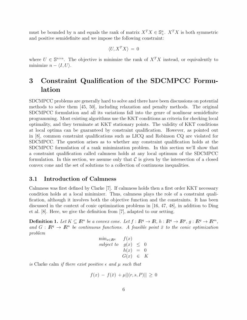
SDCMPCC problems are generally hard to solve and there have been discussions on potentialmethods to solve them [45, 50], including relaxation and penalty methods. The originalSDCMPCC formulation and all its variations fall into the genre of nonlinear semidefiniteprogramming. Most existing algorithms use the KKT conditions as criteria for checking localoptimality, and they terminate at KKT stationary points. The validity of KKT conditionsat local optima can be guaranteed by constraint qualification. However, as pointed outin [8], common constraint qualifications such as LICQ and Robinson CQ are violated forSDCMPCC. The question arises as to whether any constraint qualification holds at theSDCMPCC formulation of a rank minimization problem. In this section we’ll show thata constraint qualification called calmness holds at any local optimum of the SDCMPCCformulation. In this section, we assume only that C is given by the intersection of a closedconvex cone and the set of solutions to a collection of continuous inequalities.

3.1 Introduction of Calmness

Calmness was first defined by Clarke [7]. If calmness holds then a first order KKT necessarycondition holds at a local minimizer. Thus, calmness plays the role of a constraint quali-fication, although it involves both the objective function and the constraints. It has beendiscussed in the context of conic optimization problems in [16, 47, 48], in addition to Dinget al. [8]. Here, we give the definition from [7], adapted to our setting.

Definition 1. Let K ⊆ IRn be a convex cone. Let f : IRq → IR, h : IRq → IRp, g : IRq → IRm,and G : IRq → IRn be continuous functions. A feasible point x to the conic optimizationproblem

minx∈IRq f(x)subject to g(x) ≤ 0

h(x) = 0G(x) ∈ K

is Clarke calm if there exist positive ε and µ such that

f(x) − f(x) + µ||(r, s, P )|| ≥ 0

6

whenever ||(r, s, P )|| ≤ ε, ||x− x|| ≤ ε, and x satisfies the following conditions:

h(x) + r = 0, g(x) + s ≤ 0, G(x) + P ∈ K.

The idea of calmness is that when there is a small perturbation in the constraints, theimprovement in the objective value in a neighborhood of xmust be bounded by some constanttimes the magnitude of perturbation.

Theorem 1. [8] If calmness holds at a local minimizer x of (4) then the following first ordernecessary KKT conditions hold at x:

there exist multipliers λh ∈ Rp, λg ∈ IRm, ΩG ∈ Sn+, ΩH ∈ Sn+, and λc ∈ IR suchthat the subdifferentials of the constraints and objective function of (4) satisfy

0 ∈ ∂f(x) + ∂〈h, λh〉(x) + ∂〈g, λg〉(x)

+ ∂〈G,ΩG〉(x) + ∂〈H,ΩH〉(x) + λc∂c(x),

λg ≥ 0, 〈g(x), λg〉 = 0, ΩG ∈ Sn+, ΩH ∈ Sn+,〈ΩG, G(x)〉 = 0, 〈ΩH , H(x)〉 = 0.

In the framework of general nonlinear programming, previous results [27] show that theMangasarian-Fromowitz constraint qualification (MFCQ) and the constant-rank constraintqualification (CRCQ) imply local calmness. When all the constraints are linear, CRCQwill hold. However, in the case of SDCMPCC, calmness may not hold at locally optimalpoints. Linear semidefinite programming programs are a special case of SDCMPCC: takeH(x) identically equal to the zero matrix. Even in this case, calmness may not hold. Forlinear SDP, the optimality conditions in Theorem 1 correspond to primal and dual feasibilitytogether with complementary slackness, so for example any linear SDP which has a dualitygap or where dual attainment fails will not satisfy calmness. Consider the example below,where we show explicitly that calmness does not hold:

minimizex1,x2

x2

s.t G(x) =

x2 + 1 0 00 x1 x2

0 x2 0

0(11)

It is trivial to see that any point (x1, 0) with x1 ≥ 0 is a global optimal point to the problem.However:

Proposition 1. Calmness does not hold at any point (x1, 0) with x1 ≥ 0.

Proof. We will omit the case when x1 > 0 and only show the proof for the case x1 = 0.Take

x1 = δ and x2 = −δ2

7

As δ → 0, we can find a matrix:

M =

1− δ2 0 00 δ −δ2

0 −δ2 δ3

0

in the semidefinite cone and||G(δ,−δ2)−M || = δ3.

However, the objective value at (δ,−δ2) is −δ2. Thus we have:

f(x1, x2) − f(0, 0)

||G(δ,−δ2)−M ||=

−δ2

||G(δ,−δ2)−M ||≤ −δ

2

δ3→ −∞

as δ → 0. It follows that calmness does not hold at the point (0, 0) since µ is unbounded.

3.2 Calmness of SDCMPCC Formulation

In this part, we would like to show that in Problem (7), calmness holds for each pair (X,U)with X feasible and U given by (9). The variable x in (4) is equal to the pair (X,U) from (7),so G(x) = X and H(x) = U . We assume

C = Sn+ ∩ X : gi(X) ≤ 0, i = 1, . . . ,m1

for continuous functions gi(X); these functions are incorporated into g(x) in the formula-tion (4). Before presenting the propositions, we introduce the rank constrained problem forany positive integer k:

minX∈Sn+ ψ(X)

subject to X ∈ C (RC(k))rank(X) ≤ k.

Proposition 2. Let X be a local minimizer of (RC(k)) for some choice of k and let U begiven by (9). Then (X,U) is a local optimal solution in Problem (7). Conversely, if (X,U) isa local optimal solution to (7) then U is given by (9) and X is a local minimizer of (RC(k))with k = rank(X).

Proof. The proposition follows from the fact that rank(X ′) ≥ rank(X) for all X ′ close enoughto X.

Proposition 3. For any local minimizer X of (RC(k)) for some choice of k with U given

8

by (9), let (X, U) be a feasible point to the optimization problem below:

minimizeX,U ∈ Sn

n − 〈I, U〉 + ψ(X)

subject to X + p ∈ C

|〈X, U〉| ≤ q

λmin(I − U) ≥ −r

λmin(X) ≥ −h1

λmin(U) ≥ −h2

(12)

where p, q, r, h1 and h2 are perturbations to the constraints and λmin(M) denotes theminimum eigenvalue of matrix M . Assume X has at least one positive eigenvalue. For||(p, q, r, h1, h2)||, ||X − X||, and ||U − U || all sufficiently small, we have

〈I, U〉 − 〈I, U〉 ≥ −2q

λ− (n− rank(X))

(r + (1 + r) 2

λh1

)−h2

(4λ||X||∗ − rank(X)

) (13)

where ||X||∗ is the nuclear norm of X and λ is the smallest positive eigenvalue of X.

Proof. The general scheme is to determine a lower bound for 〈I, U〉 and an upper boundfor 〈I, U〉. A lower bound of 〈I, U〉 can be easily found by exploiting the complementarityconstraints and its value is n− rank(X). To find an upper bound of 〈I, U〉, the approach wetake is to fix X in Problem (12) and estimate a lower bound for the objective value of thefollowing problem:

minimizeU ∈ Sn

n − 〈I, U〉

subject to −〈X, U〉 ≤ q, y1

〈X, U〉 ≤ q, y2

I − U −r I, Ω1

U −h2 I, Ω2

(14)

where y1, y2, Ω1 and Ω2 are the Lagrangian multipliers for the corresponding constraints. Itis obvious that (X, U) must be feasible to Problem (14). We find an upper bound for (I, U)

9

by finding a feasible solution to the dual problem of Problem (14), which is:

maximizey1,y2∈R,Ω1,Ω2 ∈ Sn

n + q y1 + q y2 − (1 + r) trace(Ω1) − h2 trace(Ω2)

subject to −y1 X + y2 X − Ω1 + Ω2 = −I

y1, y2 ≤ 0

Ω1, Ω2 0

(15)

We can find a lower bound on the dual objective value by looking at a tightened version,which is established by diagonalizing X by linear transformation and restricting the non-diagonal term of Ω1 and Ω2 to be 0. Let fi, gi be the entries on the diagonal of Ω1 andΩ2 after the transformation respectively, and λi be the eigenvalues of X. The tightenedproblem is:

maximizey1,y2∈R, f, g ∈Rn

n + q y1 + q y2 − (1 + r)∑

i fi − h2

∑i gi

subject to −y1 λi + y2 λi − fi + gi = −1, ∀i = 1 · · ·n

y1, y2 ≤ 0

fi, gi ≥ 0, ∀i = 1 · · ·n

(16)

By proper assignment of the value of y1, y2, f, g, we can construct a feasible solution to thetightened problem and give a lower bound for the optimal objective of the dual problem.Let λi be the set of eigenvalues of X, with λ the smallest positive eigenvalue, and set:

y1 = 0 and y2 = −2

λ

For f and g:

• if λi <λ2, take fi = 1 + y2λi, gi = 0.

• if λi ≥ λ2, take fi = 0 and gi = 2

λλi − 1.

It is trivial to see that the above assignment will yield a feasible solution to Problem (16)and hence a lower bound for the dual objective is:

n − 2q

λ−∑λi<

λ2

(1 + r)(1 + y2λi) − h2

∑λi≥ λ2

(2

λλi − 1) (17)

By weak duality the primal objective value must be greater or equal to the dual objectivevalue, thus:

n− 〈I, U〉 ≥ n − 2q

λ−∑λi<

λ2

(1 + r)(1 + y2λi) − h2

∑λi≥ λ2

(2

λλi − 1).

10

Since we can writen− 〈I, U〉 = n −

∑λi=0

1,

it follows that for ||U − U || sufficiently small we have

(n− 〈I, U〉) − (n− 〈I, U〉) ≥ n − 2q

λ−∑λi<

λ2

(1 + r)(1 + y2λi)

−h2

∑λi≥ λ2

( 2λλi − 1) − (n −

∑λi=0

1)

= −2q

λ−∑λi<

λ2

(r + (1 + r)y2λi)

−h2

∑λi≥ λ2

( 2λλi − 1).

(18)

For λi <λ2, by the constraints λi ≥ −h1 and setting y2 = − 2

λ, we have:

r + (1 + r)y2λi ≤ r + (1 + r)2h1

λ.

For λi ≥ λ2, recall the definition for nuclear norm and we have:∑

λi≥ λ2

λi ≤ 2||X||∗

for ||X − X|| sufficiently small. Since there are exactly n − rank(X) eigenvalues in X thatconverge to 0, we can simplify the above inequality(18) and have:

(n− 〈I, U〉) − (n− 〈I, U〉) ≥ −2q

λ− (n− rank(X))(r + (1 + r)2h1

λ)

−h2

(4λ||X||∗ − rank(X)

).

(19)

Thus we can prove the inequality.

There is one case that is not covered by Proposition 3, namely that X = 0. This is alsocalm, as we show in the next lemma.

Lemma 1. Assume X = 0 is feasible in (7), with U given by (9). Let (X, U) be a feasiblepoint to (12). We have

(n− 〈I, U〉) − (n− 〈I, U〉) ≥ −nr.

Proof. Note that 〈I, U〉 = n, since X = 0 and U satisfies (9). In addition, each eigenvalueof U is no larger than 1 + r, so the result follows.

11

Proposition 4. Calmness holds at each (X,U) provided (i) X is a local minimizer of (RC(k))for some choice of k and (ii) U is given by (9).

Proof. This follows directly from Proposition 3, Lemma 1, and the Lipschitz continuityassumption on ψ(X).

It follows that any local minimizer of the SDCMPCC formulation of the rank minimiza-tion problem is a KKT point. Note that no assumptions are necessary regarding C.

Theorem 2. The KKT condition of Theorem 1 holds at each local optimum of Problem (7).

Proof. This is a direct result from Theorem 1 and Propositions 2 and 4.

The above results show that, similar to the exact complementarity formulation of `0

minimization, there are many KKT stationary points in the exact SDCMPCC formulationof rank minimization, so it is possible that an algorithm will terminate at some stationarypoint that might be far from a global optimum. As we have shown in the complementarityformulation for `0 minimization problem [11], a possible approach to overcome this difficultyis to relax the complementarity constraints. In the following sections we investigate whetherthis approach works for the SDCMPCC formulation.

4 A Penalty Scheme for SDCMPCC Formulation

In this section and the following sections, we present a penalty scheme for the originalSDCMPCC formulation. The penalty formulation has the form:

minimizeX,U ∈ Sn

n − 〈I, U〉+ ψ(X) + ρ〈X, U〉 =: fρ(X,U)

subject to X ∈ C

0 I − U

X 0

U 0

(20)

We denote the problem as SDCPNLP (ρ). We discuss properties of the formulation inthis section, with an algorithm described in Section 5 and computational results given inSection 6. First, we note that it follows from standard results that a sequence of globalminimizers to (20) converges to a global optimizer of (7); see Luenberger [28] for example.

From now on, we assume

C = X ∈ Sn : 〈Ai, X〉 = bi, i = 1, . . . ,m2,

where each Ai ∈ Sn, so C is an affine manifold.

12

4.1 Constraint Qualification of Penalty Formulation

The penalty formulation for the Rank Minimization problem is a nonlinear semidefiniteprogram. As with the exact SDCMPCC formulation, we would like to investigate whetheralgorithms for general nonlinear semidefinite programming problems can be applied to solvethe penalty formulation. As far as we know, most algorithms in nonlinear semidefiniteprogramming use first order KKT stationary conditions as the criteria for termination. TheKKT stationary condition at a local optimum of the penalty formulation is:

0 U ⊥ −I + Ψ + ρX + Y 0

0 X ⊥∑λiAi + ρU 0

0 Y ⊥ I − U 0

(21)

for X ∈ C, where λ ∈ IRm2 are the dual multipliers corresponding to the linear constraintsY ∈ Sn+ are the dual multipliers corresponding to the constraints I − U 0, and Ψ isa subgradient of ψ(X). Unfortunately, the counterexample below shows that the KKTconditions do not hold in the penalty problem (20) in general:

minimizeX,U ∈ S3,x∈R

3 − 〈I, U〉 + ρ 〈X,U〉

subject to X =

3 + x 0 00 1− x x

2

0 x2

0

0 I − U

X 0

U 0

(22)

Every feasible solution requires x = 0. It is obvious that if ρ = 0.5 then the optimal solutionto the above problem is:

x = 0, X =

3 0 00 1 00 0 0

and U =

0 0 00 1 00 0 1

and the optimal objective value is 1.5. However, there does not exist any KKT multiplierat this point. We can show explicitly that calmness is violated at the current point. If weallow λmin(X) ≥ −h1 and λmax(U) ≤ 1 + h1, then we can take

x =√h1, X =

3 +√h1 0 0

0 1−√h1

√h1/2

0√h1/2 0

and U =

0 0 00 1 −h1

0 −h1 1

.13

It is obvious that (x,X, U)→ (x, X, U) as h1 → 0. The resulting objective value at (x,X, U)is 1.5 − 0.5

√h1 − 0.5h1.5

1 . Thus, for small h1, the difference in objective function value isO(√h1), while the perturbation in the constraints is only O(h1), so calmness does not hold.

Lack of constraint qualification indicates that algorithms such as the Augmented La-grangian method may not converge in general if applied to the penalty formulation. How-ever, if we enforce a Slater constraint qualification on the feasible region of X, we show belowthat calmness will hold in the penalty problem (20) at local optimal points.

Proposition 5. Calmness holds at the local optima of the penalty formulation (20) if Ccontains a positive definite matrix.

Proof. Since the Slater condition holds for the feasible regions of both X and U , for each pair(Xl, Ul) in the perturbed problem we can find (Xl, Ul) in C ∩ Sn+ with the distance between

(Xl, Ul) and (Xl, Ul) bounded by some constant times the magnitude of perturbation.In particular, let (X, U) be a strictly feasible solution to (20) with minimum eigen-

value δ > 0. Let the minimum eigenvalue of (Xl, Ul) be −ε < 0. We construct

(Xl, Ul) = (Xl, Ul) +ε

δ + ε

((X, U) − (Xl, Ul)

)∈ Sn+.

Note that for ε << δ, we have

fρ(Xl, Ul) − fρ(Xl, Ul) = O(ε),

exploiting the Lipschitz continuity of Ψ(X). As (Xl, Ul) converges to (X, U), we also have(Xl, Ul)→ (X, U), so by the local optimality of (X, U) we can give a bound on the optimalvalue of the perturbed problem and the statement holds.

It follows that the KKT conditions will hold at local minimizers for the penalty formu-lation.

Proposition 6. The first order KKT condition holds at local optimal solutions for the penaltyformulation (20) if the Slater condition holds for the feasible region C ∩ Sn+ of X.

4.2 Local Optimality Condition of Penalty Formulation

4.2.1 Property of KKT Stationary Points of Penalty Formulation

The KKT condition in the penalty formulation works in a similar way with some thresholdingmethods [5, 6, 43, 44]. The objective function not only counts the number of zero eigenvalues,but also the number of eigenvalues below a certain threshold, as illustrated in the followingproposition.

Proposition 7. Let (X, U) be a local optimal solution to the penalty formulation. Let σi bean eigenvalue of U and vi be a corresponding eigenvector of norm one. It follows that:

• If σi = 1, then vTi (Ψ + ρX)vi ≤ 1.

14

• If σi = 0, then vTi (Ψ + ρX)vi ≥ 1.

• if 0 < σi < 1, then vTi (Ψ + ρX)vi = 1

Proof. If σi = 1, since vi is an eigenvector of U, by the complementarity in the KKTcondition it follows that:

vTi (−I + Ψ + ρX + Y )vi = 0.

As vTi Y vi ≥ 0, we have vTi (Ψ + ρX)vi ≤ 1.If σi = 0, then vi is an eigenvector of I − U with eigenvalue 1. By the complementarity

of I − U and Y we have vTi Y vi = 0 and

vTi (−I + Ψ + ρX + Y )vi = −1 + vTi (Ψ + ρX)vi ≥ 0.

The above inequality is satisfied if and only if vTi (Ψ + ρX)vi ≥ 1.If 0 < σi < 1,then vi is an eigenvector of I −U corresponding to an eigenvalue in (0, 1).

The complementarity in KKT condition implies that vTi Y vi = 0 = vTi (−I + Ψ + ρX + Y )vi.It follows that vTi (Ψ + ρX)vi = 1.

Using the proposition above, we can show the equivalence between the stationary pointsof the SDCMPCC formulation and the penalty formulation.

Proposition 8. If (X, U) is a stationary point of the SDCMPCC formulation with corre-sponding subgradient Ψ then it is a stationary point of the penalty formulation if the penaltyparameter ρ is sufficiently large.

Proof. Choose ρ so that the minimum positive eigenvalue of Ψ+ρX is strictly greater than 1.By setting λ = 0 and with a proper assignment of Y we can see that first order optimalitycondition (21) holds at (X, U) for such a choice of ρ, thus (X, U) is a KKT stationary pointfor the penalty formulation.

4.2.2 Local Convergence of KKT Stationary Points

We would like to investigate whether local convergence results can be established for thepenalty formulation, that is, whether the limit points of KKT stationary points of the penaltyscheme are KKT stationary points of the SDCMPCC formulation. Unfortunately, localconvergence does not hold for the penalty formulation, although the limit points are feasiblein the original SDCMPCC formulation.

Proposition 9. Let (Xk, Uk) be a KKT stationary point of the penalty scheme with subgra-dient Ψk and penalty parameter ρk. As ρk → ∞, any limit point (X, U) of the sequence(Xk, Uk) is a feasible solution to the original problem.

Proof. The proposition can be verified by contradiction. Note that the norm of Ψk is boundedsince ψ(X) is Lipschitz continuous. If the Frobenius inner product of X and U is greaterthan 0, then when k is large enough we have:

〈Uk,−Ik + Ψk + ρkXk + Yk〉 ≥ −〈Uk, I〉 + 〈Uk,Ψk〉 + ρk〈Xk, Uk〉 > 0

which violates the complementarity in the KKT conditions of the penalty formulation.

15

We can show that a limit point may not be a KKT stationary point. Consider thefollowing problem:

minimizeX,U ∈ S3+

n − 〈I, U〉

subject to X11 = 1, 0 U I and 〈U,X〉 = 0(23)

The penalty formulation takes the form:

minimizeX,U ∈ S2+

n − 〈I, U〉 + ρk〈X,U〉

subject to X11 = 1, 0 U I(24)

Let Xk and Uk take the value:

Xk =

[1 00 2

ρk

], Uk =

[0 00 0

],

so (Xk, Uk) is a KKT stationary point for the penalty formulation. However, the limit point:

X =

[1 00 0

], Uk =

[0 00 0

],

is not a KKT stationary point for the original SDCMPCC formulation.

5 Proximal Alternating Linearized Minization

The proximal alternating linearized minimization (PALM) algorithm of Bolte et al. [3] isused to solve a wide class of nonconvex and nonsmooth problems of the form

minimizex∈IRn,y∈IRm Φ(x, y) := f(x) + g(y) + H(x, y) (25)

where f(x), g(y) and H(x, y) satisfy smoothness and continuity assumptions:

• f : Rn → (−∞,+∞] and g : Rm → (−∞,+∞] are proper and lower semicontinuousfunctions.

• H: Rn × Rm → R is a C1 function.

No convexity assumptions are made. Iterates are updated using a proximal map with respectto a function σ and weight parameter t:

proxσt (x) = argminx∈Rd

σ(x) +

t

2||x − x||2

. (26)

When σ is a convex function, the objective is strongly convex and the map returns a uniquesolution. The PALM algorithm is given in Procedure 1. It was shown in [3] that it convergesto a stationary point of Φ(x, y) under the following assumptions on the functions:

16

input : Initialize with any (x0, y0) ∈ Rn × Rm. Given Lipschitz constants L1(y) andL2(x) for the partial gradients of H(x, y) with respect to x and y.

output: Solution to (25).

For k = 1, 2, · · · generate a sequence xk, yk as follows:

• Take γ1 > 1, set ck = γ1L1(yk) and compute: xk+1 ∈ proxfck(xk − 1

ck∇xH(xk, yk)).

• Take γ2 > 1, set dk = γ2L2(xk) and compute: yk+1 ∈ proxgdk(yk − 1

dk∇yH(xk, yk)).

Procedure 1: PALM algorithm

• infRm×Rn Φ > −∞, infRn f > −∞ and infRm g > −∞.

• The partial gradient ∇xH(x, y) is globally Lipschitz with moduli L1(y), so:

||∇xH(x1, y)−∇xH(x2, y)|| ≤ L1(y)||x1 − x2||, ∀x1, x2 ∈ Rn.

Similarly, the partial gradient ∇yH(x, y) is globally Lipschitz with moduli L2(x).

• For i = 1, 2, there exists λ−i , λ+i such that:

– infL1(yk) : k ∈ N ≥ λ−1 and infL2(xk) : k ∈ N ≥ λ−2

– supL1(yk) : k ∈ N ≤ λ+1 and supL2(xk) : k ∈ N ≤ λ+

2 .

• ∇H is continuous on bounded subsets of Rn×Rm, i.e, for each bounded subset B1×B2

of Rn × Rm there exists M > 0 such that for all (xi, yi) ∈ B1 ×B2, i = 1, 2:

||(∇xH(x1, y1)−∇xH(x2, y2),∇yH(x1, y1)−∇yH(x2, y2), )||≤ M ||(x1 − x2, y1 − y2)||.

(27)

The PALM method can be applied to the penalty formulation of SDCMPCC formulationof rank minimization (20) with the following assignment of the functions:

f(X) = 12ρX ||X||2F + ψ(X) + I(X ∈ C)

g(U) = n − 〈I, U〉 + I(U ∈ 0 U I)H(X, U) = ρ〈X, U〉,

where I(.) is an indicator function taking the value 0 or +∞, as appropriate. Note that wehave added a regularization term ||X||2F to the objective function. When the feasible regionfor X is bounded, the assumptions required for the convergence of the PALM procedure holdfor the penalty formulation of SDCMPCC.

Proposition 10. The function Φ(X,U) = f(X) + g(U) + H(X,U) is bounded below forX ∈ Sn and U ∈ Sn if ψ(X) is bounded below.

17

Proof. Since the eigenvalues of U are bounded by 1, and the Frobenius norm of X and Umust be nonnegative, the statement is obvious.

Proposition 11. If the feasible region of X is bounded then H(X,U) is globally Lipschitiz.

Proof. The gradient of H(X,U) is:

(∇XH(X,U),∇UH(X,U)) := ρ(U,X)

The statement results directly from the boundedness of the feasible region of X and U .

Proposition 12. ∇H(X,U) = ρ(U, X) is continuous on bounded subsets of Sn × Sn.

The proximal subproblems in Procedure 1 are both convex quadratic semidefinite pro-grams. The update to Uk+1 has a closed form expression based on the eigenvalues andeigenvectors of Uk − (ρ/dk)X

k. Rather than solving the update problem for Xk+1 directlyusing, for example, CVX [13], we found it more effective to solve the dual problem usingNewton’s method, with a conjugate gradient approach to approximately solve the direction-finding subproblem. This approach was motivated by work of Qi and Sun [35] on findingnearest correlation matrices. The structure of the Hessian for our problem is such that theconjugate gradient approach is superior to a direct factorization approach, with matrix-vectorproducts relatively easy to calculate compared to formulating and factorizing the Hessian.The updates to X and U are discussed in Sections 5.2 and 5.3, respectively. First, we discussaccelerating the PALM method.

5.1 Adding Momentum Terms to the PALM Method

One downside for proximal gradient type methods are their slow convergence rates. Nes-terov [32, 33] proposed accelerating gradient methods for convex programming by adding amomentum term. The accelerated algorithm has a quadratic convergence rate, comparedwith sublinear convergence rate of the normal gradient method. Recent accelerated proximalgradient methods include [37, 42].

Bolte et al. [3] showed that the PALM proximal gradient method can be applied tononconvex programs under certain assumptions and the method will converge to a localoptimum. The question arises as to whether there exists an accelerated version in nonconvexprogramming. Ghadimi et al. [12] presented an accelerated gradient method for nonconvexnonlinear and stochastic programming, with quadratic convergence to a limit point satisfyingthe first order KKT condition.

There are various ways to set up the momentum term [21, 23]. Here we adopted thefollowing strategy while updating xk and yk:

xk+1 ∈ proxfck(xk − 1

ck∇xH(xk, yk) + βk(xk − xk−1)). (28)

yk+1 ∈ proxgdk(yk − 1

dk∇yH(xk, yk) + βk(yk − yk−1)), (29)

where βk = k−2k+1

(borrowing from [33]). We refer to this as the Fast PALM method.

18

5.2 Updating X

Assume C = X ∈ Sn : A(X) = b, X 0 and the Slater condition holds for C. Theproximal point X of X, or proxfck(X) can be calculated as the optimal solution to theproblem:

minimizeX ∈ Sn

ρX ||X||2F + ψ(X) + ck||X − X||2F

subject to A(X) = bX 0

(30)

The objective can be replaced by:

||X − ckck + ρX

X||2F +1

ρXψ(X).

With the Fast PALM method, we use

X = Xk − ρ

ckUk + βk(Xk −Xk−1).

We observed that the structure of the subproblem to get the proximal point is very similarto the nearest correlation matrix problem when ψ(X) ≡ 0. Qi and Sun [35] showed that forthe nearest correlation matrix problem, a semismooth Newton’s method is numerically veryefficient compared to other existing methods, and it achieves a quadratic convergence rate ifthe Hessian at the optimal solution is positive definite. Provided Slater’s condition holds forthe feasible region of the subproblem and its dual program, strong duality holds and insteadof solving the primal program, we can solve the dual program which has the following form:

minyθ(y) :=1

2||(G +A∗y)+||2F − bTy

where (M)+ denotes the projection of the symmetric matrix M ∈ Sn onto the cone of positivesemidefinite matrices Sn+, and

G =ck

ck + ρXX.

One advantage of the dual program over the primal program is that the dual program isunconstrained. Newton’s method can be applied to get the solution y∗ which satisfies thefirst order optimality condition:

F (y) := A (G + A∗y)+ = b. (31)

Note that ∇θ(y) = F (y)− b. The algorithm is given in Procedure 2.In each iteration, one key step is to construct the Hessian matrix Vk. Given the eigenvalue

decompositionG + A∗y = PΛP T ,

19

input : Given y0, η ∈ (0, 1), ρ, σ. Initialize k = 0.output: Solution to (31).

For each k = 0, 1, 2, · · · generate a sequence yk+1 as follows:

• Select Vk ∈ ∂F (yk) and apply the conjugate gradient method [14] to find anapproximate solution dk to:

∇θ(yk) + Vkd = 0

such that:||∇θ(yk) + Vkd

k|| ≤ ηk||∇θ(yk)||.

• Line Search. Choose the smallest nonnegative integer mk such that:

θ(yk + ρmdk) − θ(yk) ≤ σρm∇θ(yk)Tdk.

• Set tk := ρmk and yk+1 := yk + tkdk.

Procedure 2: Newton’s method to solve (31)

let α, β, γ be the sets of indices corresponding to positive, zero and negative eigenvalues λirespectively. Set:

My =

Eαα Eαβ (τij)i∈α,j∈βEβα 0 0

(τji)i∈α,j∈β 0 0

where all the entries in Eαα, Eαβ and Eβα take value 1 and

τij :=λi

λi − λj, i ∈ α, j ∈ γ

The operator Vy : Rm → Rm is defined as:

Vyh = A(P (My (P T (A∗h)P ))P T

),

where denotes the Hadamard product. Qi and Sun [35] showed

Proposition 13. The operator Vy is positive semidefinite, with 〈h, Vyh〉 ≥ 0 for any h ∈ Rm.

Since positive definiteness of Vy is required for the conjugate gradient method, a pertur-bation term is added in the linear system:

(Vy + εI)dk + ∇θ(yk) = 0.

After getting the dual optimal solution y∗, the primal optimal solution X∗ can be recoveredby:

X∗ = (G + A∗y∗)+.

20

5.3 Updating U

The subproblem to update U is:

minimizeU ∈ Sn

n − 〈I, U〉 + dk2||U − U ||2F

subject to 0 U I,

withU = Uk − ρ

dkXk + βk(Uk − Uk−1)

with the Fast PALM method. The objective is equivalent to minimizing ||U − (U + 1dkI)||2F .

An analytical solution can be found for this problem. Given the eigenvalue decompositionof U + 1

dkI:

U +1

dkI =

n∑i=1

σUi vivTi ,

the optimal solution U∗ is:

U∗ =n∑i=1

σU∗

i vivTi

where the eigenvalue σU∗

i takes the value:

σU∗

i =

0 if σUi < 0

σUi if 0 ≤ σUi ≤ 1

1 if σUi > 1

Note also that

U∗ = I −n∑i=1

(1− σU∗

i ) vivTi .

It may be more efficient to work with this representation if there are many more eigenvaluesat least equal to one as opposed to less than zero.

6 Test Problems

Our experiments included tests on coordinate recovery problems [1, 9, 20, 34, 38]. In theseproblems, the distances between items in IR3 are given and it is necessary to recover thepositions of the items. Given an incomplete Euclidean distance matrix D = (d2

ij), where:

d2ij = dist(xi, xj)

2 = (xi − xj)T (xi − xj),

we want to recover the coordinate xi, i = 1, · · · , n. Since the coordinate is in 3-dimensionalspace, xi, i = 1, · · · , n is a 1 × 3 vector. Let X = (x1, x2, · · · , xn)T ∈ Rn×3. The problem

21

turns into recovering the matrix X. One way to solve the problem is to lift X by introducingB = XXT and we would like to find B that satisfies

Bii + Bjj − 2Bij = d2ij, ∀(i, j) ∈ Ω

where Ω is set of pairs of points whose distance has been observed. Since X is of rank 3, therank of the symmetric psd matrix B is 3, and so we seek to minimize the rank of B in theobjective.

We generated 20 instances and in each instance we randomly sampled 150 entries froma 50 × 50 distance matrix. We applied the PALM method and the Fast PALM methodto solve the problem. For each case, we limit the maximum number of iterations to 200.Figures 1 and 2 each show the results on 10 of the instances. As can be seen, the Fast PALMapproach dramatically speeds up the algorithm. The computational tests were conductedusing Matlab R2013b running in Windows 10 on an Intel Core i7-4719HQ CPU @2.50GHzwith 16GB of RAM.

We compared the rank of the solutions returned by the fast PALM method for (20) withthe solution returned by the convex nuclear norm approximation to (6). Note that whenwe calculate the rank of the resulting X in both the convex approximation and the penaltyformulation, we count the number of eigenvalues above the threshold 0.01. Figure 3 showsthat when 150 distances are sampled, the solutions returned by the penalty formulationhave notably lower rank when compared with the convex approximation. There was onlyone instance where the penalty formulation failed to find a solution with rank 3; in contrast,the lowest rank solution found by the nuclear norm approach had rank 5, and that was onlyfor one instance.

We also experimented with various numbers of sampling distances from 150 to 195. Foreach number, we randomly sampled that number of distances, then compared the averagerank returned by the penalty formulation and the convex approximation. Figure 4 showsthat the penalty formulation is more likely to recover a low rank matrix when the numberof sampled distances is the same. The nuclear norm approach appears to need about 200sampled distances in order to obtain a solution with rank 3 in most cases. There has beensome research on maximizing the nuclear norm os symmetric matrices to approximatelyminimize rank [19]. However, for our (very sparse) instances we obtained similar rankseither minimizing or maximizing the nuclear norm.

For the 20 cases where 150 distances are sampled, the average time for CVX is 0.6590seconds, while for the penalty formulation the average time for the fast PALM method is10.21 seconds. Although the fast PALM method cannot beat CVX in terms of speed, it cansolve the problem in a reasonable amount of time and produces a lower rank solution for ourtest instances.

7 Conclusions

The SDCMPCC approach gives an equivalent nonlinear programming formulation for thecombinatorial optimization problem of minimizing the rank of a symmetric positive semidefi-

22

Figure 1: Computational Results for 10 distance recovery instances. The objective value for thetwo methods at each iteration is plotted. If the algorithm terminates before the iteration limit, theobjective value after termination is 0 in the figure.

23

Figure 2: Computational Results of Case 11-20

24

Figure 3: Rank of solutions when 150 distances are sampled for 20 instances with 150×150 distancematrix.

25

Figure 4: Average rank of solutions for the 20 instances, as the number of sampled distancesincreases from 150 to 195.

26

nite matrix subject to convex constraints. The disadvantage of the SDCMPCC approach liesin the nonconvex complementarity constraint, a type of constraint for which constraint qual-ifications might not hold. We showed that the calmness constraint qualification holds for theSDCMPCC formulation of the rank minimization problem, provided the convex constraintssatisfy an appropriate condition. We developed a penalty formulation for the problem whichsatisfies calmness under the same condition on the convex constraint. The penalty formula-tion could be solved effectively using an alternating direction approach, accelerated throughthe use of a momentum term. For our test problems, our formulation outperformed a nuclearnorm approach, in that it was able to recover a low rank matrix using fewer samples thanthe nuclear norm approach.

There are alternative nonlinear approaches to rank minimization problems, and it wouldbe interesting to explore the relationships between the methods. The formulation we’vepresented is to minimize the rank; the approach could be extended to handle problems withupper bounds on the rank of the matrix, through the use of a constraint on the trace ofthe additional variable U . Also of interest would be the extension of the approach to thenonsymmetric case.

References

[1] A. Y. Alfakih, M. F. Anjos, V. Piccialli, and H. Wolkowicz, Euclidean dis-tance matrices, semidefinite programming, and sensor network localization, PortugaliaeMathematica, 68 (2011), pp. 53–102.

[2] L. Bai, J. E. Mitchell, and J. Pang, On conic QPCCs, conic QCQPs and com-pletely positive programs, Mathematical Programming, 159 (2016), pp. 109–136.

[3] J. Bolte, S. Sabach, and M. Teboulle, Proximal alternating linearized minimiza-tion for nonconvex and nonsmooth problems, Mathematical Programming, 146 (2014),pp. 459–494.

[4] O. Burdakov, C. Kanzow, and A. Schwartz, Mathematical programs with cardi-nality constraints: reformulation by complementarity-type conditions and a regulariza-tion method, SIAM Journal on Optimization, 26 (2016), pp. 397–425.

[5] J.-F. Cai, E. J. Candes, and Z. Shen, A singular value thresholding algorithm formatrix completion, SIAM Journal on Optimization, 20 (2010), pp. 1956–1982.

[6] L. Cambier and P.-A. Absil, Robust low-rank matrix completion by Riemannianoptimization, SIAM Journal on Scientific Computing, 38 (2016), pp. S440–S460.

[7] F. H. Clarke, Optimization and Nonsmooth Analysis, SIAM, Philadelphia, PA, USA,1990.

27

[8] C. Ding, D. Sun, and J. Ye, First order optimality conditions for mathematical pro-grams with semidefinite cone complementarity constraints, Mathematical Programming,147 (2014), pp. 539–579.

[9] Y. Ding, N. Krislock, J. Qian, and H. Wolkowicz, Sensor network localiza-tion, euclidean distance matrix completions, and graph realization, Optimization andEngineering, 11 (2008), pp. 45–66.

[10] M. Fazel, H. Hindi, and S. P. Boyd, A rank minimization heuristic with applicationto minimum order system approximation, in Proceedings of the 2001 American ControlConference, June 2001, IEEE, 2001, pp. 4734–4739, https://faculty.washington.

edu/mfazel/nucnorm.html.

[11] M. Feng, J. E. Mitchell, J. Pang, X. Shen, and A. Wachter, Complementar-ity formulations of `0-norm optimization problems, tech. report, Department of Math-ematical Sciences, Rensselaer Polytechnic Institute, Troy, NY, 2013. Revised: May2016.

[12] S. Ghadimi and G. Lan, Accelerated gradient methods for nonconvex nonlinear andstochastic programming, Mathematical Programming, 156 (2016), pp. 59–99.

[13] M. Grant, S. Boyd, and Y. Ye, Disciplined convex programming, in Global Op-timization: From Theory to Implementation, L. Liberti and N. Maculan, eds., Non-convex Optimization and its Applications, Springer-Verlag Limited, Berlin, Germany,2006, pp. 155–210.

[14] M. R. Hestenes and E. Stiefel, Methods of Conjugate Gradients for Solving LinearSystems, NBS, Bikaner, India, 1952.

[15] C.-J. Hsieh and P. Olsen, Nuclear norm minimization via active subspace selection,in Internat. Conf. Mach. Learn. Proc., Beijing, China, 2014, pp. 575–583.

[16] X. X. Huang, K. L. Teo, and X. Q. Yang, Calmness and exact penalization in vec-tor optimization with cone constraints, Computational Optimization and Applications,35 (2006), pp. 47–67.

[17] R. H. Keshavan, A. Montanari, and S. Oh, Matrix completion from a few entries,IEEE Transactions on Information Theory, 56 (2010), pp. 2980–2998.

[18] M. Kocvara and M. Stingl, PENNON – a code for convex nonlinear and semidefi-nite programming, tech. report, Institute of Applied Mathematics, University of Erlan-gen, Erlangen, Germany, 2002.

[19] N. Krislock and H. Wolkowicz, Euclidean distance matrices and applications,in Handbook on Semidefinite, Conic and Polynomial Optimization, M. Anjos andJ. Lasserre, eds., International Series in Operational Research and Management Sci-ence, Springer, 2012, pp. 879–914.

28

[20] M. Laurent, A tour d’horizon on positive semidefinite and Euclidean distance matrixcompletion problems, in Topics in Semidefinite and Interior Point Methods, vol. 18 ofThe Fields Institute for Research in Mathematical Sciences, Communications Series,AMS, Providence, Rhode Island, 1998.

[21] H. Li and Z. Lin, Accelerated proximal gradient methods for nonconvex programming,in Adv. Neural Inform. Process. Syst., Montreal, Canada, 2015, pp. 379–387.

[22] X. Li, S. Ling, T. Strohmer, and K. Wei, Rapid, robust, and reliable blind deconvo-lution via nonconvex optimization, tech. report, Department of Mathematics, Universityof California Davis, Davis, CA 95616, June 2016.

[23] Q. Lin, Z. Lu, and L. Xiao, An accelerated randomized proximal coordinate gradientmethod and its application to regularized empirical risk minimization, SIAM Journal onOptimization, 25 (2015), pp. 2244–2273.

[24] Z. Lin, M. Chen, and Y. Ma, The augmented lagrange multiplier method for exactrecovery of corrupted low-rank matrices, tech. report, Perception and Decision Lab,University of Illinois, Urbana-Champaign, IL, 2010.

[25] Y.-J. Liu, D. Sun, and K.-C. Toh, An implementable proximal point algorithmicframework for nuclear norm minimization, Mathematical Programming, 133 (2012),pp. 399–436.

[26] Z. Liu and L. Vandenberghe, Interior-point method for nuclear norm approxima-tion with application to system identification, SIAM Journal on Matrix Analysis andApplications, 31 (2009), pp. 1235–1256.

[27] S. Lu, Relation between the constant rank and the relaxed constant rank constraintqualifications, Optimization, 61 (2012), pp. 555–566.

[28] D. G. Luenberger, Linear and Nonlinear Programming, 2nd edition, Addison-Wesley,Menlo Park, 1984.

[29] S. Ma, D. Goldfarb, and L. Chen, Fixed point and Bregman iterative methods formatrix rank minimization, Mathematical Programming, 128 (2011), pp. 321–353.

[30] K. Mohan and M. Fazel, Reweighted nuclear norm minimization with applicationto system identification, in Amer. Control Conf. Proc., Baltimore, MD, 2010, IEEE,pp. 2953–2959.

[31] K. Mohan and M. Fazel, Iterative reweighted algorithms for matrix rank minimiza-tion, Journal of Machine Learning Research, 13 (2012), pp. 3441–3473.

[32] Y. Nesterov, Introductory Lectures on Convex Optimization: A Basic Course,Springer Science & Business Media, New York, NY, USA, 2013.

29

[33] Y. E. Nesterov, A method for unconstrained convex minimization problem with therate of convergence o(1/k2), Doklady AN SSSR, 269 (1983), pp. 543–547. translated asSoviet Mathematics Doklady.

[34] T. K. Pong and P. Tseng, (Robust) edge-based semidefinite programming relaxationof sensor network localization, Mathematical Programming, 130 (2011), pp. 321–358.

[35] H. Qi and D. Sun, A quadratically convergent Newton method for computing the near-est correlation matrix, SIAM Journal on Matrix Analysis and Applications, 28 (2006),pp. 360–385.

[36] B. Recht, M. Fazel, and P. A. Parrilo, Guaranteed minimum-rank solutionsof linear matrix inequalities via nuclear norm minimization, SIAM Review, 52 (2010),pp. 471–501.

[37] M. Schmidt, N. L. Roux, and F. R. Bach, Convergence rates of inexact proximal-gradient methods for convex optimization, in Adv. Neural Inform. Process. Syst.,Granada, Spain, 2011, pp. 1458–1466.

[38] A. M.-C. So and Y. Ye, Theory of semidefinite programming for sensor networklocalization, Mathematical Programming, 109 (2007), pp. 367–384.

[39] N. Srebro and T. Jaakkola, Weighted low-rank approximations, in Internat. Conf.Mach. Learn. Proc., Atlanta, GA, 2003, pp. 720–727.

[40] R. Sun and Z.-Q. Luo, Guaranteed matrix completion via nonconvex factorization,in 2015 IEEE 56th Annual Symposium on Foundations of Computer Science, 2015,pp. 270–289.

[41] J. Tanner and K. Wei, Low rank matrix completion by alternating steepest descentmethods, Applied and Computational Harmonic Analysis, 40 (2016), pp. 417–429.

[42] K. C. Toh and S. Yun, An accelerated proximal gradient algorithm for nuclear normregularized linear least squares problems, Pacific Journal of Optimization, 6 (2010),pp. 615–640.

[43] B. Vandereycken, Low-rank matrix completion by Riemannian optimization, SIAMJournal on Optimization, 23 (2013), pp. 1214–1236.

[44] K. Wei, J.-F. Cai, T. F. Chan, and S. Leung, Guarantees of Reimannian op-timization for low rank matrix completion, tech. report, Department of Mathematics,University of California at Davis, CA, USA, April 2016.

[45] J. Wu and L. Zhang, On properties of the bilinear penalty function method for math-ematical programs with semidefinite cone complementarity constraints, Set-Valued andVariational Analysis, 23 (2015), pp. 277–294.

30

[46] H. Yamashita and H. Yabe, A survey of numerical methods for nonlinear semidef-inite programming, Journal of the Operations Reseach Society of Japan, 58 (2015),pp. 24–60.

[47] J. J. Ye and J. Zhou, First-order optimality conditions for mathematical programswith second-order cone complementarity constraints, tech. report, Department of Math-ematics and Statistics, University of Victoria, Victoria, BC, Canada V8W 2Y2, 2015.

[48] J. Zhai and X. X. Huang, Calmness and exact penalization in vector optimizationunder nonlinear perturbations, Journal of Optimization Theory and Applications, 162(2014), pp. 856–872.

[49] H. Zhang, Z. Lin, and C. Zhang, A counterexample for the validity of using nuclearnorm as a convex surrogate of rank, in Machine Learning and Knowledge Discovery inDatabases, Springer, Berlin, Germany, 2013, pp. 226–241.

[50] Y. Zhang, L. Zhang, and J. Wu, Convergence properties of a smoothing approachfor mathematical programs with second-order cone complementarity constraints, Set-Valued and Variational Analysis, 19 (2011), pp. 609–646.

31