Embed Size (px)
Citation preview
Queueing SystDOI 10.1007/s11134-012-9317-7
A performance analysis of channel fragmentationin dynamic spectrum access systems
Ed Coffman · Philippe Robert · Florian Simatos ·Shuzo Tarumi · Gil Zussman
Received: 12 September 2011 / Revised: 8 November 2011© The Author(s) 2012. This article is published with open access at Springerlink.com
Abstract Dynamic Spectrum Access systems offer temporarily available spectrumto opportunistic users capable of spreading transmissions over a number of non-contiguous subchannels. Such methods can be highly beneficial in terms of spectrumutilization, but excessive fragmentation degrades performance and hence off-sets thebenefits. To get some insight into acceptable levels of fragmentation, we present ex-perimental and analytical results derived from a mathematical model. According tothe model, a system operates at capacity serving requests for bandwidth by assigninga collection of one or more gaps of unused bandwidth to each request as bandwidthbecomes available. Our main result is a proof that, even if fragments can be arbitrarilysmall, the system remains stable in the sense that the average total number of frag-ments remains bounded. Within the class of dynamic fragmentation models, includ-
This paper is a revision for journal publication of the conference paper [3]. All of the results hereincan be found in [3].
E. Coffman · S. Tarumi · G. ZussmanElectrical Engineering, Columbia University, New York, NY, USA
E. Coffmane-mail: [email protected]
S. Tarumie-mail: [email protected]
G. Zussmane-mail: [email protected]
P. RobertINRIA Paris-Rocquencourt, Paris, Francee-mail: [email protected]
F. Simatos (�)CWI, Amsterdam, The Netherlandse-mail: [email protected]

Queueing Syst
ing models of dynamic storage allocation that have been around for many decades,this result appears to be the first of its kind.
In addition, we provide extensive experimental results that describe behavior, attimes unexpected, of fragmentation as parameter values are varied. Different scan-ning rules for searching gaps of available spectrum, all covered by the above stabilityresult, are also studied. Our model applies to dynamic linked-list storage allocation,and provides a novel analysis in that domain. We prove that, interestingly, a versionof the 50 % rule of the classical, non-fragmented allocation model holds for the newmodel as well. Overall, the paper provides insights into the behavior of practical frag-mentation algorithms.
Keywords Dynamic spectrum access · Fragmentation · Ergodicity of Markovchains · Cognitive radio · Lyapunov function
Mathematics Subject Classification 60J20
1 Introduction
This paper focuses on the analysis of dynamic resource allocation algorithms andis motivated by applications of these algorithms to Dynamic Spectrum Access Net-works (also known as Cognitive Radio Networks). Cognitive Radios can adapt theirtransmitter parameters to the environment in which they operate and are viewed askey enablers of efficient use of the underutilized wireless spectrum [1, 7, 8, 17]. Un-der the basic model of Cognitive Radio Networks [1], Secondary Users (SUs) areallowed to use white spaces (also known as spectrum holes) that are not used by thePrimary Users but must avoid interfering with active Primary Users (for instance, seeFig. 1).
An SU’s channel allocation may be broken down into a number of subchannels,each allocated to a distinct hole of unused bandwidth. As shown in Fig. 1, this canbe realized, for example, by employing a variant of Orthogonal Frequency-DivisionMultiplexing (OFDM) [10, 15, 18–20, 22]. Although the physical-layer aspects ofOFDM-based Dynamic Spectrum Access have been extensively studied recently, al-lowing channel fragmentation introduces several new problems [12, 20, 23] that sig-nificantly differ from classical Medium Access Control (MAC).1
Fig. 1 Non-contiguous OFDM with Primary and Secondary Users (SUs), where the Secondary Users usenon-contiguous channels that do not overlap with the Primary Users’ channels
1Further details on Dynamic Spectrum Access Networks can be found in [3], which also contains anextensive review of related work.

Queueing Syst
In this paper, we study a baseline theoretical model in which the spectrum isshared by SUs only. Those users have to transmit and receive data, and accordinglyneed some bandwidth for given amounts of time. Hence, bandwidth requests of SUsare characterized by a desired total bandwidth and the duration of a time interval overwhich it is needed. The data transmission can take place over a non-contiguous chan-nel (i.e., a number of subchannels). Once a transmission terminates, some fragments(subchannels) are vacated, and therefore, gaps (spectrum holes/white spaces) developrandomly in both size and position. When allocating a channel to a new SU request,it is fragmented (in the frequency domain) into available gaps until the full requestedbandwidth is provided. This process repeats itself, until the next request fails to fit intothe available fragments (more details are provided in the model subsection below).
The main goal of the paper is to investigate the phenomena of fragmentation in-duced by spectrum allocation algorithms. For this purpose, we will ignore the par-ticularities of techniques such as OFDM and make a couple of assumptions (for acomplete system description, see Sect. 2): (i) the system operates at capacity andthere is always a waiting bandwidth request; and (ii) the fragment size is not boundedfrom below. Making the first assumption allows us to study the effect of fragmenta-tion in the worst case. Clearly, if there are idle periods, when there are no waitingrequests, only departures occur and the fragmentation level of the system decreasesduring these periods. Similarly, the latter assumption allows us to study the systemperformance when artificial lower bounds on the fragment size are not imposed. Thisdiffers from OFDM-based systems in which a subcarrier has a given minimal band-width.
In the application of these spectrum allocation algorithms, intriguing new prob-lems in dynamic allocation arise. For example, because of the dynamic use of thespectrum, the bandwidth available to a new user will usually be distributed amonga number of gaps in the spectrum. In principle, the random arrival and departure ofusers might cause the system to evolve in such a way that sequences of many, verysmall gaps are often allocated to user requests. In such cases, the system performancewill deteriorate, since the algorithms maintaining the state of a highly fragmentedspectrum become more time-consuming. To put these remarks on a proper footing,we first need to introduce the details of our model.
1.1 The model
A continuous frequency band of given width is made available to users. Each suchuser makes a request composed of a required total bandwidth and the duration ofa residence time for the exchange of data over a channel of this bandwidth. Chan-nels are allocated to requests on a first-come-first-served basis, subject to availablebandwidth. A channel must remain fixed while active, and on departure it returns itsallocation to the pool of available bandwidth. The channel of an allocated request isallowed to consist of multiple, disjoint bandwidth fragments, each being accommo-dated by a gap of unused spectrum that was available at the time of allocation.
For convenience, the model normalizes the spectrum to the interval [0,1], so thesizes of all bandwidth requests are numbers in [0,1]. Our goal is to characterize thefragmentation of requests when the system is operating at capacity, so we assume that

Queueing Syst
there is effectively an infinite queue of waiting users. For the purposes of the exampleto be given shortly, we denote the sizes of their bandwidth requests by u1, u2, . . . .We will also use ui as the name of the ith user. An initial, non-fragmented state isconstructed as follows. Starting at 0, consecutive subintervals of sizes u1, u2, . . . areassigned as the channels of waiting users until a request size ui , i > 1, is encounteredwhich exceeds available bandwidth, i.e.,
u1 + · · · + ui−1 ≤ 1 < u1 + · · · + ui
At this point, all i − 1 of the channels in this initial state begin their residencetimes. Subsequent state transitions take place at departure epochs when the residencetimes of currently allocated channels expire. Suppose all requests up to uj have beenallocated channels and a request ui , i ≤ j , departs, releasing its allocated channel.If there is still not enough bandwidth for uj+1, then it must wait for one or moreadditional departures. Otherwise, uj+1, uj+2, . . . are allocated their requested band-widths until, once again, a request is encountered that asks for more bandwidth thanis available. All channels then begin or continue their residence times as before untilthe next departure.
The linear-scan (LS) rule sets up a channel by scanning the spectrum in order ofincreasing frequency, allocating gaps of available bandwidth in partial fulfillment ofthe request until enough bandwidth has been allocated to satisfy the entire request.In general, the last gap is only partially used, in which case the last fragment is left-justified in the last gap. An example is shown in Fig. 2. Allocations are shown forthe first eight user requests, assuming that, at time 0, the spectrum is not in use. Therequests with sizes u1, u2, and u3 are the first to be allocated channels; u4 must waitfor a departure, since the first four request sizes sum to more than 1. The variablesti give the sequence of departure times of allocated requests. We see that the firstoccurrence of fragmentation takes place at the departure of u2 and the subsequentadmission of u4; an initial fragment of u4 is placed in the gap left by u2 and a finalfragment is placed after u3. Note also that, even after u2 and u4 have departed, thereis still not enough bandwidth for u5. After the additional departure of u1, both u5 andu6, but not u7, can be allocated bandwidth.
Fig. 2 An example of the admission and departure processes and the resulting spectrum fragmentation

Queueing Syst
We complete the model description by giving the probability laws governing theresidence times and sizes of the waiting requests. With α ∈ (0,1] a parameter of themodel, the sizes uj+1, uj+2, . . . are drawn independently from the uniform distribu-tion on (0, α]. The residence times of allocated requests are independent of requestsizes and form a sequence of i.i.d. exponentially distributed random variables. Forsimplicity, the mean is normalized to 1.
1.2 Main results
At first glance, since request sizes can be arbitrarily small, the fragments used bybandwidth requests might well become progressively narrower as time passes, inwhich case the number of fragments could grow without bound. Clearly, such anoperational model cannot be supported by a realistic system, so it is of great interestto know whether this can actually happen. The principal theoretical contribution ofthis paper is a proof that in fact, with high probability, the number of fragments in thesystem remains acceptably low. A precise statement is deferred to the next sectionwhere additional notation and concepts are introduced.
In addition to mathematical results, and in order to gain further insight into theperformance of the system, we present the results of extensive experiments. Theseshow that although for a given maximum request size α, the number of fragments hasa finite expected value, there is a linear relationship between 1/α and the expectednumber of fragments into which a request is divided. This indicates that when therequests are constrained to be small, they are also fragmented into a relatively largenumber of fragments. From a practical point of view, this implies that, if we canimpose a lower bound on the fragment size by rejecting gaps that are too small, thenwe have a useful control on the ill effects of excessive fragmentation.
Our experiments show that different bandwidth allocation algorithms exhibit sig-nificantly different performance in terms of the fragmentation occurring in the sys-tem. As one example, an algorithm that scans the gaps in decreasing order of theirsizes reduces the fragmentation by almost an order of magnitude compared to LS.Interestingly, the experiments also show that the number of fragments is distributedaccording to a normal law with a relatively low mean value. Finally, the experimentsfor small α led to the interesting observation that the ratio of the average numberof gaps to the average number of requests being served was approximately 1/2. Al-though we were unable to prove this ratio-of-averages result, we were able to provea corresponding 50 % limit law for the expected value of the ratio of the number ofgaps to the number of requests being served.
The spectrum allocation problems described here can be characterized in the con-text of dynamic storage allocation problems of computers; see Knuth [14]. In thatcontext, the term “spectrum” refers to the storage unit, “bandwidth requirements”refer to storage requirements, and “channel” refers to a region in storage contain-ing a file. In the original dynamic storage model, fragmentation referred only tothe gaps of unoccupied storage interspersed with intervals of occupied storage: fileswere not fragmented. The reader familiar with that model may have found the 50 %rule observed in our experiments to be reminiscent of Knuth’s 50 % rule, which as-serts that the number of gaps is approximately half the number of files when exact
Queueing Syst
fits of files into gaps are rare. Our notion of fragmentation applies also to the filesthemselves, so our discovery that a similar 50 % rule continued to apply was a sur-prising one at first. Note that, in terms of the storage application, our model corre-sponds precisely to linked-list allocation of files—channels allocated to requests aresets of linked, disjoint segments of storage allocated to file fragments. Our resultsprovide a novel analysis for such systems, and have implications for the garbage-collection/defragmentation process in linked-list systems. We note that studies of dy-namic storage allocation have been around for some 40 years, and widely recognizedas posing very challenging problems to both combinatorial and stochastic modelingand analysis. In particular, results of the type found in this paper, rigorous withinstochastic models, seem to be quite new.
The remainder of the paper begins in the next section with the introduction of no-tation, a formalization of the spectrum state space, and the stochastic processes ofinterest in later sections. Section 3 presents experimental results that bring out theeffects of fragmentation, particularly as a function of the maximum request size α.In Sect. 4 relations between variables describing the configuration of gaps and frag-ments are proved in preparation for (1) a 50 % limit law for the relation betweenthe number of active channels and the number of gaps in the spectrum at departuretimes, and (2) our main stability result, which shows that the expected value of thetotal number of fragments and gaps is bounded. These results are proved in Sects. 4and 5, respectively. Section 5 also proves that, for α large enough, an equilibriumdistribution exists. Section 6 discusses algorithmic issues, such as changes in perfor-mance resulting from alternative allocation algorithms, and Sect. 7 discusses experi-mental results that exhibit normal approximations for the total number of fragmentsand gaps. Section 8 concludes the paper with a discussion of the results and futureresearch directions.
2 Preliminaries
The state of a fragmentation process must carry the information given by a sequenceof gaps alternating with sequences of contiguous fragments. Accordingly, we formal-ize a state space S for our model as follows.
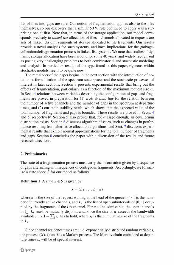
Definition 1 A state x ∈ S is given by
x = (L1, . . . ,Lr ;u)
where u is the size of the request waiting at the head of the queue, r ≥ 1 is the num-ber of currently active channels, and Li is the list of open subintervals of [0,1] occu-pied by the fragments of the ith channel. For x to be admissible, the open intervalsin
⋃i Li must be mutually disjoint, and, since the size of u exceeds the bandwidth
available, u > 1 − ∑i si has to hold, where si is the cumulative size of the fragments
in Li .
Since channel residence times are i.i.d. exponentially distributed random variables,the process (X(t)) on S is a Markov process. The Markov chain embedded at depar-ture times tn will be of special interest.
Queueing Syst
When treated as a random variable, the size of the request waiting to be allocatedbandwidth at time t is denoted by U(t). Similarly, Ui(t) denotes a random variablegiving the size of the ith request behind the head of the queue. Except for Sect. 5,the dependence on time will usually be omitted. We denote by R(t) the number ofrequests with an active channel at time t . F(t) and G(t) denote, respectively, thenumbers of fragments and gaps at time t .
With this notation, we are in position to state our main contribution to mathemat-ical foundations. We prove that the total number of gaps and fragments at departureepochs has bounded exponential moments, as follows: For some η > 0 and any initialstate x ∈ S ,
supn≥1
Ex
(eη(F (tn)+G(tn))
)< +∞
where Ex denotes expectation for the process X started at X(0) = x. While our choiceof a uniform distribution for request sizes is a useful one, it is not essential to thisresult; it holds for more general distributions. The result shows that the sum F(tn) +G(tn) is strongly concentrated near the origin. This fact provides strong support forthe informal assertion made in Sect. 1 to the effect that, with high probability, the levelof fragmentation stays reasonably low. Our analysis has several basic ingredients:relations between the number of fragments and gaps in the spectrum (Lemma 2); adrift relation of Lyapunov type for the total number of gaps, fragments, and requests(Proposition 1); a general inequality for Markov chains (Theorem 4); and a stabilityresult of [13].
The last of these results refers to the early work of Kipnis and Robert [13] on anon-fragmented version of our model. Channel allocations can be moved as needed inorder to put all available bandwidth together in one block, so fragmentation is avoidedentirely. They consider a system with arrivals, but with arrival rates sufficiently high,their analysis of maximum throughput gives us an analysis of (R(tn)), assuming thatthe same probability laws for request sizes and residence times apply. This followssimply from the fact that the admission criterion for waiting requests is the samein both models. A major result in [13] asserts the existence and uniqueness of aninvariant measure for (R(tn)). Explicit formulas are hard to come by, but those in [13]for the maximal departure rate in special cases have provided useful checks for ourexperiments.
In Sect. 6, we shall also evaluate two scanning alternatives to LS. The first is cir-cular scan (CS), which is still a linear scan of the gaps, but each scan starts wherethe previous one left off; after the last gap in [0,1], CS cycles back to the first gapin [0,1]. The second is largest-first-scan (LFS), which is intended to further reducefragmentation by assigning gaps in order of decreasing size. Although these algo-rithms make different scans of the gap sequence, they are all alike in their treatmentof the last gap occupied: the last fragment is left-justified in the last gap. This is akey assumption, and it is very likely to hold in practice. In our probability model,it follows that, with probability 1, the last gap used in a channel allocation will bechanged to a fragment and a smaller residual gap.

Queueing Syst
3 Experimental results
The experimental study reported in this section serves two related roles. First, itbrings out characteristics of the fragmentation process that need to be borne in mindin implementations, particularly where these characteristics show parameter valuesthat must be avoided, if a system with fragmentation is to operate efficiently. Thesecond role is that of experimental mathematics, in which results indicate where be-havior might well be formalized and rigorously proved as a contribution to mathe-matical foundations. In the latter role, this section leads up to the next two sections,which formalize and prove the stability of the fragmentation process.
The experiments were conducted with a discrete-event simulator written in C thatalso includes a stochastic arrival process, a capability that we intend to explore infuture research. The maximum request size α is the single parameter surviving thenormalizations of the simpler mathematical model of this paper. The simulations weremost demanding, of course, for small α, when large numbers of departure events wereneeded to ensure behavior near the stationary regime. For every α value chosen in theinterval [0.01,1], 20 million departure events were simulated starting in an emptystate, with data collected for the last 10 million events. For every choice of α in[0.001, 0.01], 100 million departure events were processed and data collection wasperformed during the last 50 million events. The excellent accuracy of this tool wasestablished in tests against exact results for special classes of queueing systems, andagainst the maximum throughput results derived in [13]. Examples of the test resultscan be found in the appendix and in [21].
The results for the average number of channels, the average number of gaps, andthe average number of fragments per channel are shown in Fig. 3. The curves arenearly linear in 1/α for small values of α; indeed, the errors in the linear fits arewithin the thickness of the printed lines. In particular, the asymptotic (as α → 0)average number of channels in the spectrum is 2/α. When requests are large relativeto the spectrum (i.e., for α > 1/3), the behavior is not given by functions quite sosimple. As such cases are of less practical interest, we omit the relevant data.
The asymptotic linear growth of the average number of channels as a function ofchannel size is obvious, but the linearity of the other two measures is not so obvious.A closer look shows that the average number of gaps is almost exactly one half the
Fig. 3 Average numbers ofchannels, of gaps, and offragments per channel

Queueing Syst
Fig. 4 Average total number offragments vs.1/α: a quadratic fit
Fig. 5 Percentage of type-ifragments
average number of channels for even relatively small 1/α. This is the unexpected ver-sion of Knuth’s 50 % rule that we mentioned in Sect. 1. We return to this behavior inthe next section, where we prove a 50 % limit law. The linear growth of the averagenumber of fragments per channel may also be unexpected at first glance: the frag-mentation of channels increases as the average channel size decreases. This lineargrowth implies the quadratic growth of the average total number of fragments plottedin Fig. 4 (the accuracy of the fit is as before: the error is within the thickness of theprinted lines).
The analysis in later sections will focus largely on tracking fragment types definedas follows: a fragment is of type i, if it is adjacent to i other fragments, where i = 0,1, or 2. It can be seen in Fig. 5 that for small α, more than 90 % of the fragmentsare type-2 fragments. In addition, clearly, the number of type-0 and type-1 fragmentsis a function of the number of gaps. These observations and the results illustrated inFigures 3 and 4 indicate that, even for relatively small 1/α, the average total numberof type-0 and type-1 fragments grows linearly in 1/α, but the average number oftype-2 fragments grows quadratically.
Figure 6 compares the average gap and fragment sizes. As might be expected, forrelatively small α, they are close to each other. The relation holds even for moderatelylarge α, although for α rather close to 1, the difference amounts to about a factor of 2.

Queueing Syst
Fig. 6 Average sizes offragments and gaps
With this property and the 50 % rule suggested by Fig. 3, the linear growth in thenumber of fragments per channel (shown in Fig. 3) is easily explained for moderatelysmall α in the following way.
As mentioned above, for moderately small α, the number of channels is approxi-mately 2/α (i.e., the spectrum size divided by the average request size). By the 50 %rule, the number of gaps is roughly 1/α. At any time, the total size of the gaps is atmost α, since there is a request waiting for departures whose requested bandwidthexceeds the total size of the gaps. Therefore, at most α available bandwidth is spreadamong 1/α gaps, giving an average gap size on the order of α2. The average fragmentsize is at most (and indeed very close to) the average gap size. The fragments mustoccupy at least 1 − α of the spectrum since, as mentioned above, at most a fractionα of the spectrum is devoted to gaps. Thus, the number of fragments must be on theorder of 1/α2, and so the average number of fragments per channel must be on theorder of (in particular, linear in) 1/α. As α → 0, the asymptotics of these estimatesbecome more precise.

Queueing Syst
4 Numbers of fragments and gaps
This section presents analytical results relating the numbers of fragments and gapsunder the fragmentation process (X(t)). Recall the definition of fragment types:For i = 0, 1 or 2, a fragment is said to be of type i if it touches exactly i otherfragments.Ni(t) denotes the number of type i fragments at time t , so that F(t) =N0(t) + N1(t) + N2(t) is the total number of fragments.
Let σ(t) denote the sum of the numbers of fragments and gaps,
σ(t) = F(t) + G(t). (1)
The number of gaps and the numbers of fragment types are related as follows.
Lemma 1 With probability 1,
G(t) = N0(t) + 1
2N1(t) + I (t) (2)
for any t ≥ 0, where I (t) = 1, if there is a gap starting at the origin, and 0 otherwise.
Proof Each gap, except for boundary gaps starting at 0 or ending at 1, separates twofragments. Two gaps surround a type-0 fragment not touching the origin, only onetouches a type-1 fragment not touching the origin, and none touch a type-2 fragment,so the gaps strictly inside (0,1) are double-counted in 2N0(t) + N1(t). Gaps at theboundaries are counted only once in this expression, so if there are gaps touchingeach boundary, 2 must be added to 2N0(t) + N1(t) to produce a double count of allgaps. Then N0(t) + N1(t)/2 + 1 counts the gaps as called for by the lemma.
With probability 1, a gap always touches the boundary at 1, so the only case leftto consider is the absence of a gap touching the origin. In this case, there is a type-0or type-1 fragment touching the origin, and so a nonexistent gap has been counted in2N0(t) + N1(t). This over-count cancels the under-count of the gap touching 1, andso no correction term is needed, i.e., N0(t) + N1(t)/2 counts all gaps as stated in thelemma. �
Definition 2 Let (tk) denote the sequence of departure times, let Di(tk) denote thenumber of type i fragments in the channel leaving at time tk , and let A(tk) denote thenumber of requests admitted to the spectrum at time tk . Finally, define the drift in thetotal number of fragments and gaps:
�σ(tk)def= σ(tk) − σ(tk−1) (3)
with the convention t0 = Di(t0) = Ai(t0) = 0.
The following lemma is the basis of the stability analysis of σ(t) in Sect. 5, andthe 50 % rule proved later in this section.

Queueing Syst
Lemma 2 With probability 1, the departure at tk creates the following change in thetotal number of fragments and gaps:
�σ(tk) = A(tk) − 2D0(tk) − D1(tk) + J (tk), k ≥ 1 (4)
with t0 = 0, and J (tk) = 1, if a fragment starting at the origin is in the departingchannel, and 0 otherwise.
Proof With probability 1, each new channel allocation covers completely every gapit is allocated, except for the last one, which is only partially covered. Thus, withprobability 1, each new channel allocation changes gaps to fragments, except for thelast gap which is changed to a fragment plus a gap; this adds one to σ(tk−1) for eachadmission, which accounts for the total of A(tk) in (4).
Two fragments of the same channel cannot be contiguous, so it is correct to addup the changes created by departing fragments, with each being treated separately.Suppose first that there is no fragment (0, b) against the origin. Then for every type-0fragment in the departing channel, two gaps and a fragment are replaced by a singlegap for a net decrease of two, and for every departing type-1 fragment, a gap anda fragment are replaced by a single gap for a net reduction of one. This gives thereduction of 2D0(tk) + D1(tk) appearing in (4). If there is a fragment (0, b), it mustbe of type 0 or 1; if it is of type 0, then its departure gives a decrease of one; if itis of type 1, its departure has no effect. Each of these contributions is one less thanit would be were the fragment not touching the origin. There can only be one suchfragment, so the correction shown in J (tk) for a fragment (0, b) follows. �
We will denote by G−(tk) the total number of gaps just after the kth departure,but before new admissions, if any, are made. Note that if we remove A(tk) from theright-hand side of (4) and add back the total number of departing fragments at tk , i.e.,D0(tk) + D1(tk) + D2(tk), we get the number of gaps available to admissions at thekth departure:
G−(tk) = G(tk−1) − D0(tk) + D2(tk) + J (tk) (5)
with J (tk) = 1 as in Lemma 2.Knuth’s widely known 50 % rule appears in a very different context than the model
here, so it is difficult to anticipate the apparent fact that it also holds for our fragmen-tation model. However, one can argue a similar result assuming that the fragmentationprocess has a stationary distribution. The result is given below as an expected valueof a ratio, rather than a ratio of expected values.
Theorem 1 Assume that for each α > 0, the fragmentation process at departureepochs (X(tk), k ≥ 0) with request sizes uniformly distributed in (0, α) admits atleast one stationary distribution. For each α > 0 pick one stationary distribution πα .Then
limα→0
Eπα
(G(0)
R(0)
)
= 1
2.

Queueing Syst
Proof Any stationary distribution πα must satisfy Eπα [σ(t1)] = Eπα [σ(t0)] andEπα [A(t1)] = 1. Thus, using Lemma 2 one gets
Eπα
[2D0(t1) + D1(t1) − J (t1)
] = 1. (6)
Now for a state x having R(0) > 0 channels and Ni(0) type-i (i = 0,1,2) fragments,we have from Lemma 1
Ex
[2D0(t1) + D1(t1) − J (t1)
] = (2N0(0) + N1(0)
)/R(0) − Ex
[J (t1)
]
= 2[G(0) − I (0)
]/R(0) − Ex
[J (t1)
].
The term Ex[J (t1)] is equal to the probability that a fragment starting at the originleaves. This is certainly smaller than the probability that the channel with the frag-ment closest to the origin leaves, which by symmetry is equal to 1/R(0). Using inaddition I (0) = 0 or 1 one gets
0 ≤ 1
2− Eπα
(G(0)/R(0)
) ≤ 2Eπα
(1/R(0)
).
Now for any stationary distribution πα the random variable R(0) under πα must bedistributed according to the stationary distribution of the non-fragmented model ofKipnis and Robert [13], and one easily checks that Eπα (1/R(0)) goes to 0 as α goesto 0, hence the result. �
Note that, because we have a Lyapunov function (see Proposition 1), the exis-tence of a stationary distribution would be guaranteed if we could prove that theprocess (X(tn)) has the Feller property, see for instance Proposition 12.1.3 in Meynand Tweedie [16].
5 Stability results
This section establishes that the average total number of fragments and gaps remainsbounded and that, for certain distributions of request sizes, ergodicity holds. The anal-ysis leads to the following two results. Recall that (tn) is the sequence of departuretimes (t0 = 0) and σ(t) = F(t)+G(t), defined in (1), is the total number of fragmentsand gaps.
Theorem 2 There exists some η > 0 such that, for any initial state x ∈ S ,
supn≥1
Ex
(eησ(tn)
)< +∞. (7)
Clearly, this implies that for any initial state x ∈ S , the sequence (Ex(σ (tn)),n ≥ 0) is bounded. With an additional assumption on the distribution of the requestsize, a stronger stability result can be proved.
Theorem 3 When α > 1/2, the process (X(t)) is positive Harris recurrent; in par-ticular, it has a unique stationary distribution.

Queueing Syst
A criterion for finite exponential moments using a Lyapunov function is estab-lished next. Then, we provide some estimates of the drift of the number of fragmentsbetween departures which will show us how to construct such a Lyapunov function.The proofs of Theorems 2 and 3 will finally be given in Sects. 5.4 and 5.5.
5.1 A criterion for finite exponential moments
Before stating the main result, some results on Markov chains are needed. In the se-quel, ≤st refers to stochastic ordering, i.e., V ≤st Z means that E(f (V )) ≤ E(f (Z))
for any increasing function f . For reasons that will become clear in Lemma 5, thefollowing lemma focuses on admissions at four consecutive departure times. Recallthat (Ui, i ≥ 1) are the sizes of the requests waiting to be allocated bandwidth afterU , the first one, and that they are assumed to be i.i.d.
Lemma 3 The random variable A(t1)+ · · ·+A(t4) is stochastically dominated by arandom variable Z such that E(eλZ) < +∞ for some λ > 0.
Proof It is clear that A(t1) ≤ Z + 1 where
Z = 1 + inf{n ≥ 1 : U1 + · · · + Un ≥ 1}.Markov’s inequality shows that for any z ≥ 0,
P(Z ≥ z + 1) = P(U1 + · · · + Uz ≤ 1) ≤ e(E
(e−U1
))z
and so E(eηZ) is finite for η > 0 small enough. From this observation, it is not difficultto extend the result to A(t1) + · · · + A(t4) instead of just A(t1). �
This lemma shows in particular that
ξdef= sup
i≥1supx∈S
Ex
(A(ti)
)< +∞.
is well-defined; this constant will be used repeatedly throughout the rest of the anal-ysis. The proof of the following lemma is standard, and therefore, omitted.
Lemma 4 Let Z ≥ 0 be a positive, real-valued random variable such that E(eλZ) <
+∞ for some λ > 0, and define c = λ−2E(eλZ − 1 − λZ). Then for any 0 ≤ ε ≤ λ
and any real-valued random variable V such that V ≤st Z, we have E(eεV ) ≤ 1 +εE(V ) + ε2c.
The following result is closely related to a result of Hajek [11].
Theorem 4 Let (Yk) be a discrete-time, continuous state-space Markov chain suchthat for some function f ≥ 0, there exist K,γ > 0 such that for any initial state y withf (y) > K , the inequality Ey(f (Y1) − f (Y0)) ≤ −γ holds. Assume that there existsa random variable Z such that for any initial state y, Z dominates stochastically the

Queueing Syst
random variable f (Y1) − f (Y0) under Py . Assume finally that E(eλZ) < +∞ forsome λ > 0. Then there exist η > 0 and 0 ≤ C < +∞ such that for any initial state y,
supn≥1
Ey
(eηf (Yn)
) ≤ eηf (y) + C.
Proof For any 0 < ε ≤ λ,
Ey
(eεf (Yn+1)
) = Ey
(EYn
(eε(f (Y1)−f (Y0))
)eεf (Yn)1{f (Yn)≤K}
)
+ Ey
(EYn
(eε(f (Y1)−f (Y0))
)eεf (Yn)1{f (Yn)>K}
). (8)
Since by assumption, f (Y1) − f (Y0) under Py is stochastically dominated by Z forevery y, one gets
EYn
(eε(f (Y1)−f (Y0))
) ≤ E(eεZ
) = E(eλZ
) def= D
and therefore
Ey
(EYn
(eε(f (Y1)−f (Y0))
)eεf (Yn)1{f (Yn)≤K}
) ≤ DeεK. (9)
For the second term, we apply Lemma 4 to the random variable f (Y1)−f (Y0) underPYn :
EYn
(eε(f (Y1)−f (Y0))
) ≤ 1 + εEYn
(f (Y1) − f (Y0)
) + cε2.
Thus, on the event {f (Yn) > K}, one gets
EYn
(eε(f (Y1)−f (Y0))
) ≤ 1 − γ ε + cε2 def= ρε (10)
and finally
Ey
(EYn
(eε(f (Y1)−f (Y0))
)eεf (Yn)1{f (Yn)>K}
) ≤ ρεEy
(eεf (Yn)
). (11)
Gathering the two bounds (9) and (11) in (8) finally gives
Ey
(eεf (Yn+1)
) ≤ ρεEy
(eεf (Yn)
) + DeεK
which leads by induction to
Ey
(eεf (Yn)
) ≤ ρnε eεf (y) + 1 − ρn+1
ε
1 − ρε
DeεK.
Let η = (ε/(2γ )) ∧ λ. From the definition of ρε in (10), one can easily check that0 < ρη < 1. Therefore, choosing ε = η gives the result. �
Theorem 4 will be applied to the Markov chain (X(t4n)) with a function f of the
form σκdef= σ + κR for some κ > 0 suitably chosen. (X(t4n)) is not the most natural
choice at first glance, but it appears to be needed because of the complexity of thestate space.

Queueing Syst
By Lemma 2, σ(t1) − σ(t0) ≤ A(t1) + 1 and clearly R(t1) − R(0) = A(t1) − 1, sothat
σκ(t4) − σκ(t0) ≤ (κ + 1)(A(t1) + · · · + A(t4)
) + 4
and therefore, by Lemma 3, σκ(t4) − σκ(t0) is stochastically dominated by somerandom variable Z with an exponential moment. Therefore, one has to establish anegative drift relation for σκ(t4) − σκ(t0) in order to apply Theorem 4 to the frag-mentation process (X(t4n)). This is the purpose of the following two subsections.The most delicate part is to control the term σ(t4) − σ(t0), which is the objective ofthe following section.
5.2 Evolution of the number of fragments
Let x ∈ S , the initial state of the system, have r active channels, and define the totalavailable gap size h = 1 − (s1+· · ·+sr ). Time 0, referring to the initial state x, willusually be omitted; e.g., σ(0),F (0),G(0), . . . will be simplified to σ,F,G, . . . . Thequantity �σ(tn) is defined in (3) as σ(tn) − σ(tn−1).
Lemma 5 Fix 0 < ε < 1 and 0 < η < 1/2, and let x ∈ S be an initial state such thatσ = G + F ≥ 2K + 1 for some fixed K ≥ 0.
Then F = N0 + N1 + N2 ≥ K , and
(1) If r = 1, then Ex(�σ(t1)) ≤ ξ − K .(2) If r > 1 and N0 + N1 ≥ εK , then
Ex
(�σ(t1)
) ≤ ξ + 1 − εK
r.
Assume in the remaining cases that r > 1, define K ′ = K((1 − ε)/r − ε)+, andlet i∗ ∈ {1, . . . , r} index a channel Li∗ in x with the most type-2 fragments.
(3) If N0 + N1 ≤ εK and u > h + si∗ , then
Ex
(�σ(t2)
) ≤ ξ + 2 − K ′
r(r − 1). (12)
(4) If N0 + N1 ≤ εK , u < h + si∗ and h + si∗ < ηα, then
Ex
(�σ(t3)
) ≤ ξ + 2 − (1 − η)K ′
r2(r − 1). (13)
(5) If N0 + N1 ≤ εK , u < h + si∗ and ηα < h + si∗ , then there exists a γ (η) > 0such that
Ex
(�σ(t4)
) ≤ ξ + 2 − γ (η)K ′
r5. (14)
It follows that there exists a ξ > 0 and a function ψ(r) > 0 such that for any x withσ ≥ 2K + 1,
Ex
(σ(t4) − σ
) ≤ ξ − Kψ(r). (15)

Queueing Syst
Proof As is readily verified, G ≤ F +1, so 2K +1 ≤ σ = F +G ≤ 2F +1, and henceF ≥ K as claimed. In what follows, we use repeatedly the two following simple facts:
Ex
(D0(t1) + D1(t1)
) = (N0 + N1)/r, (16)
and by Lemma 1,
G ≥ K ⇒ N0 + N1 ≥ K − 1. (17)
– First case: r = 1. In this case, right after the only channel initially present leaves,there is no channel allocated bandwidth, and therefore, σ(t1) = A(t1). Note that r = 1is only possible when α > 1/2, and in this case the possibility for a channel to bealone is crucial in the proof of the Harris recurrence stated in Theorem 3.
– Second case: r > 1, N0 + N1 ≥ εK . Under these assumptions, the inequalityfollows from (4):
Ex
(�σ(t1)
) ≤ ξ + 1 − Ex
(D0(t1) + D1(t1)
) = ξ + 1 − N0 + N1
r≤ ξ + 1 − εK
r.
In the 3 remaining cases, let N∗j denote the number of type-j fragments in
any channel i∗ which has the most type-2 fragments. If N0 + N1 ≤ εK , thensince F ≥ K , necessarily N2 ≥ (1 − ε)K and N∗
2 ≥ (1 − ε)K/r . Define the eventD∗ = {channel Li∗ leaves at t1} and recall that G− denotes the number of gaps rightafter Li∗ leaves but before new admissions, if any, are made. It follows from (5) thatG− ≥ K ′ in the event D∗, since
G− = G − N∗0 + N∗
1 + J (t1) ≥ (−εK + (1 − ε)K/r)+ = K ′.
The remaining analysis tacitly assumes that r > 1, that N0 + N1 ≤ εK , and that thechannel Li∗ leaves at t1.
– Third case: u > h + si∗ . Under this condition, A(t1) = 0, since when Li∗ leavesit does not provide enough additional bandwidth for U . In particular, R(t1) = r − 1and G(t1) = G− ≥ K ′, and so
Ex
(�σ(t2)
) ≤ ξ + 1 − Ex
(D0(t2) + D1(t2);D∗).
The strong Markov property makes it possible to lower-bound this last term.
Ex
(D0(t2) + D1(t2);D∗) = Ex
(EX(t1)
(D0(t1) + D1(t1)
);D∗)
= Ex
((N1 + N2)(t1)
R(t1);D∗
)
≥ K ′ − 1
r − 1Px
(D∗) = K ′ − 1
r(r − 1)
and therefore, Ex(�σ(t2)) ≤ ξ + 2 − K ′/(r(r − 1)).– Fourth case: u < h + si∗ < ηα. In this case U is admitted at t1. Thus it makes
sense to define the event
E4 = D∗ ∩ {U leaves at t2 and U1 > ηα}.
Queueing Syst
Then as before
Ex
(�σ(t3)
) ≤ ξ + 1 − Ex
(D0(t3) + D1(t3);E4
).
In the event E4, U is admitted at t1 and leaves at t2, while U1 stays blocked at t1 andt2, so that G(t2) = G− ≥ K ′ and R(t2) = r − 1. Hence as in the second case,
Ex
(D0(t3) + D1(t3);E4
) ≥ K ′ − 1
r − 1Px(E4) ≥ (1 − η)K ′
r2(r − 1)− 1
since Px(E4) = (1 − η)/r2. Thus (13) holds.– Fifth case: u < h + si∗ and ηα < h + si∗ . Again, U is admitted at t1. Letting Ui
denote the sizes of the requests behind U , define the event
B = {Ui < ηα, i = 1, . . . , τ and Uτ+1 > 2ηα}
with τ = inf{n ≥ 0 : U1 + · · · + Un > h + si∗ − ηα} and E′5 = D∗ ∩ B ∩
{U leaves at t2}. It is readily verified that 1 ≤ τ < +∞ almost surely. Moreover,one has in E′
5
0 < h∗ def= h + si∗ − (U1 + · · · + Uτ ) < ηα < Uτ+1.
This means that at t2, exactly τ new requests U1, . . . ,Uτ have been admitted, andUτ+1 is blocked. Moreover, for any i ∈ {1, . . . , τ }, one has h∗ + Ui < 2ηα < Uτ+1,so that if one of the τ channels allocated to the (Ui) leaves, Uτ+1 remains blocked.
When Li∗ left, there were G− ≥ K ′ gaps; in the remainder of the analysis, we callan initial gap a gap present right after Li∗ left. After Li∗ left, U and A(t1) − 1 newrequests were admitted, and then U left and A(t2) new requests were admitted at t2.Thus, at t2, each initial gap is in either of two states: either it is completely filled, orit is still a gap, i.e., it has not been filled completely. Let k be the number of initialgaps completely filled at t2, and let k′ = G− − k: then k + k′ = G− ≥ K ′. In eachinitial gap completely covered at t2, there is at least one type-2 fragment of one ofthe τ new channels. Therefore, N1,2 +N2,2 + · · ·+Nτ,2 ≥ k with Ni,2 the number oftype-2 fragments of the channel corresponding to U . In particular there is a channelLj∗ , j∗ ∈ {1, . . . , τ } with at least the average k/τ of type-2 fragments: Nj∗,2 ≥ k/τ .Define finally the event E5 = E′
5 ∩ {Lj∗ leaves at t3}. Since h∗ + Uj∗ < Uτ+1, thenUτ+1 remains blocked at t3 when E5 occurs, and therefore (note that when j∗ leaves,some gaps may merge, but not two initial gaps),
G(t3) ≥ Nj∗,2 + k′ ≥ k/τ + k′ ≥ (k + k′)/τ ≥ K ′/τ.
Now we proceed as before to obtain
Ex
(�σ(t4)
) ≤ ξ + 1 − Ex
(D0(t4) + D1(t4);E5
)
and, using the Markov property at time t3,
Queueing Syst
Ex
(D0(t4) + D1(t4);E5
) = Ex
(EX(t3)
(D0(t1) + D1(t1)
);E5)
= Ex
((N0 + N2)(t3)
R(t3);E5
)
≥ Ex
((K ′/τ − 1)+
r + τ − 2;E5
)
since R(t3) = r + τ − 2 in E5. The same kind of reasoning as before then leads to
Ex
((K ′/τ − 1)+
r + τ − 2;E5
)
≥ K ′
r5f (η,h + si∗ − αη) − 1
with the function f (η, ·) defined for y > 0 by
f (η, y) = E((
1 + τ(y))−5;B(η,y)
)
with τ(y) = inf{n ≥ 1 : U1 + · · · + Un ≥ y} and
B(η,y) = {Ui < ηα, i = 1, . . . , τ (y) and Uτ(y)+1 > 2ηα
}.
It is not difficult to show that γ (η) = inf0<y<1 f (η, y) > 0, which then gives theresult.
It remains to prove (15). One only needs to assemble the various bounds, takinginto account that Ex(�σ(ti)) ≤ ξ + 1 for any x ∈ S and i ≥ 0, to arrive at 4 separatebounds on Ex(σ (t4)−σ). For example, using the former bound for the first two termsand the last term of Ex(σ (t4) − σ) = ∑
1≤i≤4 Ex�σ(ti) and then the bound in (13)for the third term, we find that one of the four bounds, which applies when x satisfiesthe inequalities of the fourth case, is
Ex
(σ(t4) − σ
) ≤ 4ξ + 5 − (1 − η)K ′
r5
Computing the minimum over these bounds with η = 1/4 and ε = 1/r2, one ob-tains (15) after setting ξ = 4ξ + 5 and
ψ(r) = ϕ(r)
r6× (
(1 − η) ∧ γ)
with ϕ(r) = 1 − 2r−2. This concludes the proof. �
The bound (15) gives a negative drift for σ when the term Kψ(R(0)) is largeenough. But ψ(r) vanishes when r goes to infinity, and so this bound cannot yield adrift uniformly negative, the problem occurring when R(0) is large. For this reasonσ is not a Lyapunov function but the simple modification σκ = σ + κR introducedearlier is. The purpose of the additional term κR is precisely to give a negative driftwhen R(0) is large.

Queueing Syst
5.3 Construction of a Lyapunov function
Since the variation �R(tk) in the number of channels at a departure is exactly equalto A(tk) − 1, one readily gets that
σκ(t4) − σκ = (σ(t4) − σ
) + κ(A(t1) + · · · + A(t4) − 4
)
with σκ = σ +κR. In particular, if x ∈ S is such that σ ≥ 2K +1 and r = R(0) ≤ K1for some K1 ≥ 0, then (from now on, we assume without loss of generality that thefunction ψ given by (15) in Lemma 5 is decreasing)
Ex
(σκ(t4) − σκ
) ≤ ξ − Kψ(K1) + 4κ(ξ − 1)
whereas if r ≥ K1,
Ex
(σκ(t4) − σκ
) ≤ 4(ξ + 1) + κEx
(r(t4) − r
)
and so we see that we only need to control Ex(R(t4) − r) for r large. In this case,the negative drift comes from the fact that, except perhaps at t1, with high probabilitythere is no admission at a departure, since the channel that leaves is small with highprobability.
Lemma 6 There exist K1, γ1 > 0 such that if x ∈ S is such that r = R(0) ≥ K1, thenEx(R(t4) − r) ≤ −γ1.
Sketch of Proof The proof of this inequality is easier than the proof of Lemma 5, weonly give a sketch of it. From s1 + · · · + sr = 1 − h ≤ 1 one gets #{i : si ≥ γ } ≤ 1/γ ,and therefore, Px(si1 ≥ 1/
√r) ≤ 1/
√r with Li1 , i1 ∈ {1, . . . , r}, the channel that
leaves at t1. Thus, when r is large, with high probability a small channel leaves.If h − u is away from α, then the event {u1 > h − u + si1 + · · · + si4} (with ik
defined similarly) has high probability, and in this event A(t1) + · · · + A(t4) ≤ 1. Ifin contrast h − u is large, then with high probability U1 is admitted and with highprobability h−u−U1 is away from α; hence we can do the same again, and get that,with high probability, A(t1) + · · · + A(t4) ≤ 2. �
Gathering Lemma 6 and the bound (15) we can now prove that for κ suitablychosen, the function σκ = σ + κR is indeed a Lyapunov function.
Proposition 1 (Lyapunov function inequality) There exist κ and K > 0 such that ifx ∈ S is such that σκ ≥ K , then Ex(σκ(t4) − σκ) ≤ −1.
Proof Let K1 and γ1 be given by Lemma 6, and take κ and K as follows:
κ = 4ξ + 5
γ1and K = 8ξ + 2ξ + 2
ψ(K1)+ κK1 + 1.
Assume that σκ ≥ K . If r = R(0) ≥ K1, then
Ex
(σκ(t4) − σκ
) ≤ 4(ξ + 1) − κγ1 = −1.
Queueing Syst
Otherwise, r ≤ K1, and since σκ ≥ K , this necessarily gives σ ≥ K − κK1 = 2K̂ + 1with K̂ = (K − κK1 − 1)/2. Thus,
Ex
(σκ(t4) − σκ
) ≤ ξ − K̂ψ(K1) + 4ξ = −1
and the proposition follows. �
5.4 Proof of Theorem 2
Theorem 4 and Lemma 3 applied to the Markov chain (X(t4n), n ≥ 0), and the func-tion σκ show that for some η > 0 and some constant 0 ≤ C < +∞,
supn≥0
Ex
(eησκ (t4n)
) ≤ eησκ + C.
Then the Markov property gives for any i ≥ 0
supn≥0
Ex
(eησκ (t4n+i )
) ≤ Ex
(eησκ (ti )
) + C < +∞
from which (7) follows readily.
5.5 Proof of Theorem 3
In the following discussion, no conceptual argument is missing, only some formalismneeded to handle the continuous state space S . These details are routine and left tothe interested reader. In the analysis below, requests are said to be big if their sizeexceeds 1/2.
We argue that (X(t)) visits infinitely often a state in which there are no fragmentedchannels, and such that all size distributions remain the same at all visits. This isenough to show Harris recurrence; see for instance Asmussen [2]. For this purpose,it is convenient to pick a simple regeneration set E ⊂ S in which (i) the spectrumis being used by a big request, alone and with an unfragmented channel of the form(0, b), and (ii) the request U waiting at the head of the queue is also big. Each of thesehas the conditional request-size distribution given that its size is larger than 1/2, i.e.,the uniform distribution on (1/2, α), see [13].
To verify that E is visited infinitely often, consider the process (R(t),U(t)) withR(t) the number of requests allocated a channel at time t and U(t) the size of therequest at the head of the queue; the process (R(t),U(t)) is simply the process (X(t))
when the data on fragmentation is ignored. This process is positive Harris recurrent,as shown in Kipnis and Robert [13]. In particular it visits infinitely often states withR(t) = 1 and U(t) > 1/2; one can add U1(t) > 1/2 as well (i.e., the first requestin line behind the head of the queue request is also big), since this happens with ageometric probability. Then when the only channel leaves, the process (X(t)) entersE, since there is exactly one channel, it is big, it is necessarily unfragmented andof the form (0, b), and a big request is waiting at the head of the queue. Moreover,this argument shows that the time between visits to E is integrable, which in turnestablishes positive Harris recurrence. This completes the proof.

Queueing Syst
6 Algorithms
Although the focus so far has been on measures of fragmentation as a function of α,algorithmic issues are also of obvious interest. For example, more uniform patternsof gaps might be an advantage. The linear scan LS discussed in the previous sec-tions, tends to push the gaps towards the end of the spectrum, particularly when thespectrum is viewed at random times in steady state. Interestingly, our experimentshave shown that, for all α < 1/3, the starting position of the first gap in the spectrumremains very close to 0.64.
To uniformize gap locations, an alternative gap scan resembles the circular-scansequences of dynamic storage allocation [14]. In our case, circular scan (CS) usesa gap list, in which the successor to the last gap in [0,1] is the first gap in [0,1].The scan is still linear like LS, but the starting gap of the scan moves as follows: ifthe last fragment of a channel is placed in gap g, then the residual gap of g is thefirst gap scanned in constructing the next channel. Clearly, although CS will tend touniformize gap sizes as a function of position, boundary effects will persist so long asthe spectrum itself is not circular, i.e., gaps and fragments are not allowed to overlapthe end of the spectrum, a restriction that would likely be dictated in practice.
The average number of fragments per channel is a direct measure of gap-searchtimes, and one that we use here. For values of α expected to be of interest in applica-tions, the effects of a circular scan on gap-search times are only within a few percentrelative to LS, as can be seen in Fig. 7. The figure also shows the average number offragments per channel for LFS. This algorithm is designed to speed up the processof finding a set of gaps sufficient to create a new channel. It selects available gapsin a decreasing order of their sizes and allocates them to a request, thereby greed-ily minimizing the number of gaps needed to fulfill a request. The extra mechanismneeded for such a search will of course tend to reduce overall performance gains.The results in Fig. 7 for LFS show a surprisingly large improvement in the averagenumber of fragments per channel—as can be seen, a reduction by a factor more than3 is achieved for even moderately small α.
The Probability Mass Functions (pmf’s) of the number of fragments per channelare shown in Fig. 8. Notice that while all probabilities are small under LS and CS, thelargest applies to the case of no fragmentation at all. The much more peaked distribu-tion for LFS has both much smaller mean and variance: The standard deviation under
Fig. 7 Average number offragments per channel

Queueing Syst
Fig. 8 Distribution of thenumber of fragments perchannel for α = 0.1
Fig. 9 G/R → 1/2 as α → 0under LS, LFS, and CS
the linear algorithms is approximately 1.5 to 2.0 times that under LFS. The samelimiting behavior called for by the 50 % law holds for CS and LFS, which was to beexpected, as the arguments supporting the 50 % law did not depend on the sequencein which gaps were scanned. But an interesting result of our experiments with CS isthat the 50 % approximation to expectation of the ratios is within a couple of percenteven when the maximum request size is as much as one fifth of the spectrum size. Thisis easily seen in Fig. 9. The convergence rate of LFS to 50 % is intermediate betweenLS and CS.
7 Normal approximations
After the usual scaling (i.e., first centering then normalizing by the standard devi-ation), the scaled version of the number of channels, R, tends in probability to thestandard Normal, N (0,1), as M → ∞, where M = �1/α� (it is convenient to ex-press the asymptotics in this section in terms of M). This result follows easily fromthe corresponding heavy-traffic limits in [4, 5], and the ergodicity of (R(t)).
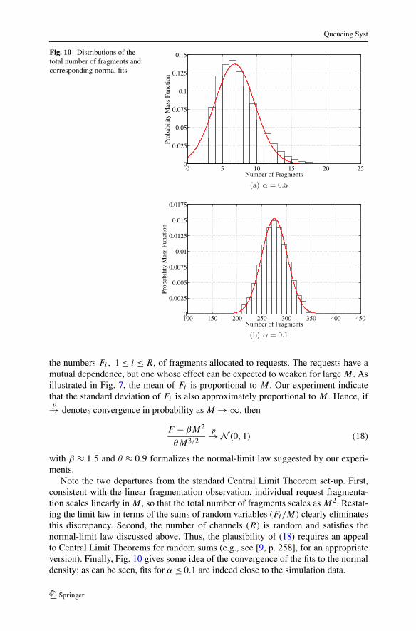
Interestingly, it was discovered in the experiments that a normal-limit law alsoappears to hold for the total number F of fragments as M → ∞ (see for exampleFig. 10). This is not surprising, since F is the sum over all requests in system of
Queueing Syst
Fig. 10 Distributions of thetotal number of fragments andcorresponding normal fits
the numbers Fi, 1 ≤ i ≤ R, of fragments allocated to requests. The requests have amutual dependence, but one whose effect can be expected to weaken for large M . Asillustrated in Fig. 7, the mean of Fi is proportional to M . Our experiment indicatethat the standard deviation of Fi is also approximately proportional to M . Hence, ifp→ denotes convergence in probability as M → ∞, then
F − βM2
θM3/2
p→ N (0,1) (18)
with β ≈ 1.5 and θ ≈ 0.9 formalizes the normal-limit law suggested by our experi-ments.
Note the two departures from the standard Central Limit Theorem set-up. First,consistent with the linear fragmentation observation, individual request fragmenta-tion scales linearly in M , so that the total number of fragments scales as M2. Restat-ing the limit law in terms of the sums of random variables (Fi/M) clearly eliminatesthis discrepancy. Second, the number of channels (R) is random and satisfies thenormal-limit law discussed above. Thus, the plausibility of (18) requires an appealto Central Limit Theorems for random sums (e.g., see [9, p. 258], for an appropriateversion). Finally, Fig. 10 gives some idea of the convergence of the fits to the normaldensity; as can be seen, fits for α ≤ 0.1 are indeed close to the simulation data.

Queueing Syst
Fig. 11 Distributions of thetotal number of fragments forα = 0.1 and the correspondingnormal fits
Fig. 12 Distributions of thenumber of gaps at differentepochs for α = 0.01
We note that the normal approximations shown for the total number of fragmentsunder LS were also found to hold under CS and LFS. This is illustrated in Fig. 11.
The distributions of the number of gaps at different epochs are shown in Fig. 12.The distribution at a random time shows a decreasing pmf. What appeared to be yetanother normal approximation was discovered when looking at the first-admissionpmf in Fig. 12; this is the distribution as seen by the first admission immediately aftera departure at just those epochs when there is at least one admission. The third curveis the pmf of the number, G−, of gaps as seen right after departures, but before deter-mining whether or not the head of the queue fits in the total available bandwidth. Thefit to the Normal density is also illustrated in the figure. The proof of a similar limitlaw for Renyi’s space-filling problem can be found in [6], but extension of knowntechniques once again faces the difficult challenges posed by our more difficult frag-mentation problem.
8 Conclusions
The results of this paper prepare the ground for further research on several fronts. Be-fore listing a number of the more important ones, we review what we have learned.Our experiments brought out first an unexpected reappearance of a 50 % rule relating

Queueing Syst
the expected numbers of gaps and channels in the limit of small request sizes relativeto the spectrum size. In our case, we were able to prove the limit law. Also, exper-imental results described a linear relationship between the inverse of the maximumrequest size, α, and the expected number of fragments into which a request was di-vided at the time of allocation. Interestingly, the smaller α was taken, the greater wasthe resulting fragmentation of requests.
Our stability results established the beginning of a mathematical foundation offragmentation processes. Particularly, we showed that for α > 1/2, the fragmen-tation process is Harris recurrent. For general α, we proved that the total num-ber of fragments is bounded in expected value. We examined alternative algo-rithms for sequencing through the available gaps and showed that using the largest-first-scan algorithm leads to significantly less fragmentation than using the linear-scan and circular-scan algorithms. Finally, we exhibited experimentally a limiting,small-α behavior in which, with appropriate scaling, distributions tend to the nor-mal.
A broad direction for further research is in extending the parameters of our math-ematical model. For instance, while Uniform distributions are generally the assump-tion of choice in fragmentation models, it would be interesting to see what new effectsare created by other distributions of request size, e.g., by varying a in the generalizeduniform distributions on [0, α], with densities xa/αa+1. The exponential residence-time assumption is likely to yield simplifications to analysis, but changes in behaviorresulting from other distributions are worth investigating. Moreover, instead of a sys-tem operating at capacity, in which there is always a request waiting, one could adoptan underlying, fully stochastic model of demand; e.g., a Poisson arrival process, asfound in [13].
More realistic, but in all likelihood significantly more difficult models, wouldrelax the independence assumptions. A prime example appropriate for DynamicSpectrum Access applications would be allowing residence times to depend onfragmentation, the greater the fragmentation of a request, the longer its residencetime.
The results regarding the performance of the different algorithms imply that thealgorithms’ design should also be considered carefully. Some examples of algorithmsthat come to mind will aim to better fit the fragments into the available gaps. A morechallenging objective would be to develop algorithms that take into account spectrumsensing capabilities during the gap allocation process.
Finally, another broad and very important avenue of research that introduces morerealistic models discretizes request sizes and the bandwidth allocation process (as isbeing done while allocating OFDM subcarriers). As in other models of fragmenta-tion, the continuous limit represented in this paper may conceal important effects, or,conversely, it may introduce effects not present in discrete models. We are activelypursuing this avenue of research.
Acknowledgements We would like to thank Charles Bordenave for helpful discussions in relation withTheorem 4. This work was partially supported by NSF grants CNS-0916263, CNS-10-54856, and CIANNSF ERC under grant EEC-0812072.
Open Access This article is distributed under the terms of the Creative Commons Attribution Licensewhich permits any use, distribution, and reproduction in any medium, provided the original author(s) andthe source are credited.
Queueing Syst
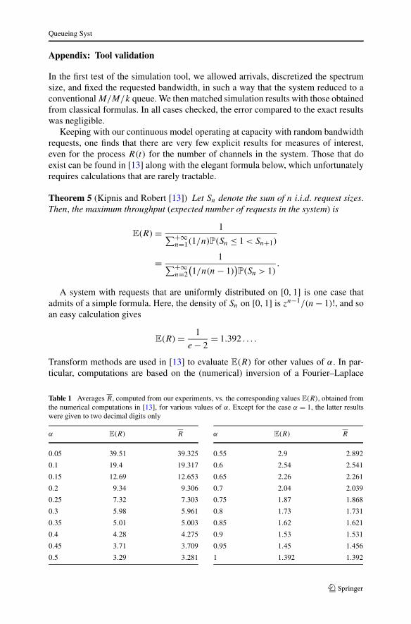
Appendix: Tool validation
In the first test of the simulation tool, we allowed arrivals, discretized the spectrumsize, and fixed the requested bandwidth, in such a way that the system reduced to aconventional M/M/k queue. We then matched simulation results with those obtainedfrom classical formulas. In all cases checked, the error compared to the exact resultswas negligible.
Keeping with our continuous model operating at capacity with random bandwidthrequests, one finds that there are very few explicit results for measures of interest,even for the process R(t) for the number of channels in the system. Those that doexist can be found in [13] along with the elegant formula below, which unfortunatelyrequires calculations that are rarely tractable.
Theorem 5 (Kipnis and Robert [13]) Let Sn denote the sum of n i.i.d. request sizes.Then, the maximum throughput (expected number of requests in the system) is
E(R) = 1∑+∞
n=1(1/n)P(Sn ≤ 1 < Sn+1)
= 1∑+∞
n=2
(1/n(n − 1)
)P(Sn > 1)
.
A system with requests that are uniformly distributed on [0,1] is one case thatadmits of a simple formula. Here, the density of Sn on [0,1] is zn−1/(n − 1)!, and soan easy calculation gives
E(R) = 1
e − 2= 1.392 . . . .
Transform methods are used in [13] to evaluate E(R) for other values of α. In par-ticular, computations are based on the (numerical) inversion of a Fourier–Laplace
Table 1 Averages R, computed from our experiments, vs. the corresponding values E(R), obtained fromthe numerical computations in [13], for various values of α. Except for the case α = 1, the latter resultswere given to two decimal digits only
α E(R) R
0.05 39.51 39.325
0.1 19.4 19.317
0.15 12.69 12.653
0.2 9.34 9.306
0.25 7.32 7.303
0.3 5.98 5.961
0.35 5.01 5.003
0.4 4.28 4.275
0.45 3.71 3.709
0.5 3.29 3.281
α E(R) R
0.55 2.9 2.892
0.6 2.54 2.541
0.65 2.26 2.261
0.7 2.04 2.039
0.75 1.87 1.868
0.8 1.73 1.731
0.85 1.62 1.621
0.9 1.53 1.531
0.95 1.45 1.456
1 1.392 1.392

Queueing Syst
transform. To evaluate the accuracy of our simulator, we checked our experimentalresults against the computations for the values of α shown in Table 1. As can be seen,the numerics agree well with simulations.
References
1. Akyildiz, I.F., Lee, W.Y., Vuran, M.C., Mohanty, S.: NeXt generation/dynamic spectrum access/cognitive radio wireless networks: a survey. Comput. Netw. 50(13), 2127–2159 (2006)
2. Asmussen, S.: Applied Probability and Queues, 2nd edn. Springer, New York (1987)3. Coffman, E., Robert, P., Simatos, F., Tarumi, S., Zussman, G.: Channel fragmentation in dynamic
spectrum access systems—a theoretical study. In: Proc. ACM SIGMETRICS’10 (2010)4. Coffman, E.G. Jr., Puhalskii, A.A., Reiman, M.I.: Storage limited queues in heavy traffic. Probab.
Eng. Inf. Sci. 5(4), 499–522 (1991)5. Coffman, E.G. Jr., Reiman, M.I.: Diffusion approximations for storage processes in computer systems.
In: Proc. ACM SIGMETRICS’83 (1983)6. Dvoretsky, A., Robbins, H.: On the ‘parking’ problem. Publ. Math. Inst. Hung. Acad. Sci. 9, 209–226
(1964)7. FCC: 03-222. Notice of proposed rulemaking (2003)8. FCC: 08-260. Second report and order, ET Docket No. 04-186, unlicensed operation in the TV broad-
cast bands (2008)9. Feller, W.: An Introduction to Probability Theory and Its Applications, vol. II, 2nd edn. Wiley, New
York (1966)10. Ghasemi, A., Sousa, E.: Spectrum sensing in cognitive radio networks: requirements, challenges and
design trade-offs. IEEE Commun. 46(4), 32–39 (2008)11. Hajek, B.: Hitting-time and occupation-time bounds implied by drift analysis with applications. Adv.
Appl. Probab. 14(3), 502–525 (1982)12. Jia, J., Zhang, Q., Shen, X.: HC-MAC: a hardware-constrained cognitive MAC for efficient spectrum
management. IEEE J. Sel. Areas Commun. 26(1), 106–117 (2008)13. Kipnis, C., Robert, P.: A dynamic storage process. Stoch. Process. Appl. 34(1), 155–169 (1990)14. Knuth, D.E.: The Art of Computer Programming. Fundamental Algorithms, vol. 1, 3rd edn. Addison
Wesley Longman Publishing Co., Redwood City (1997)15. Mahmoud, H., Yucek, T., Arslan, H.: OFDM for cognitive radio: merits and challenges. IEEE Wirel.
Commun. 16(2), 6–15 (2009)16. Meyn, S., Tweedie, R.L.: Markov Chains and Stochastic Stability, 2nd edn. Cambridge University
Press, Cambridge (2009)17. Mitola, J. III: Cognitive radio: an integrated agent architecture for software defined radio. Ph.D. thesis,
Doctor of Technology, Royal Inst. Technol. (KTH), Stockholm, Sweden (2000)18. Poston, J.D., Horne, W.D.: Discontiguous OFDM considerations for dynamic spectrum access in idle
TV channels. In: Proc. IEEE DySPAN’05 (2005)19. Rajbanshi, R., Wyglinski, A.M., Minden, G.J.: OFDM-based cognitive radios for dynamic spectrum
access networks. In: Bhargava, V.K., Hossain, E. (eds.) Cognitive Wireless Communication Networks,pp. 165–188. Springer, Berlin (2007)
20. Shukla, A., Willamson, B., Burns, J., Burbidge, E., Taylor, A., Robinson, D.: A study for the provisionof aggregation of frequency to provide wider bandwidth services. Tech. rep., QinetiQ (2006)
21. Tarumi, S.: Analysis of channel fragmentation in dynamic spectrum access networks. Ph.D. thesis,Columbia Universtiy, Electrical Engineering (2010)
22. Weiss, T.A., Jondral, F.K.: Spectrum pooling: an innovative strategy for the enhancement of spectrumefficiency. IEEE Commun. 42(3), S8–14 (2004)
23. Yuan, Y., Bahl, P., Chandra, R., Moscibroda, T., Wu, Y.: Allocating dynamic time-spectrum blocks incognitive radio networks. In: Proc. ACM MobiHoc’07 (2007)