A Permutation Test for the Regression Kink

Design�

Peter Ganong

†and Simon Jäger

‡

March 24, 2017

The Regression Kink (RK) design is an increasingly popular empirical method for estimatingcausal e�ects of policies, such as the e�ect of unemployment benefits on unemploymentduration. Using simulation studies based on data from existing RK designs, we empiricallydocument that the statistical significance of RK estimators based on conventional standarderrors can be spurious. In the simulations, false positives arise as a consequence of non-linearities in the underlying relationship between the outcome and the assignment variable,confirming concerns about the misspecification bias of discontinuity estimators pointed outby Calonico et al. (2014b). As a complement to standard RK inference, we propose thatresearchers construct a distribution of placebo estimates in regions with and without a policykink and use this distribution to gauge statistical significance. Under the assumption thatthe location of the kink point is random, this permutation test has exact size in finitesamples for testing a sharp null hypothesis of no e�ect of the policy on the outcome. Weimplement simulation studies based on existing RK applications that estimate the e�ectof unemployment benefits on unemployment duration and show that our permutation testas well as inference procedures proposed by Calonico et al. (2014b) improve upon the sizeof standard approaches, while having su�cient power to detect an e�ect of unemploymentbenefits on unemployment duration.

KEY WORDS: Randomization Inference; Permutation Test; Policy Discontinuities.

�We thank Alberto Abadie, Josh Angrist, David Card, Matias Cattaneo, Avi Feller, EdwardGlaeser, Paul Goldsmith-Pinkham, Guido Imbens, Maximilian Kasy, Zhuan Pei, Mikkel Plagborg-Møller, and Guillaume Pouliot as well as participants at Harvard University’s Research in StatisticsSeminar and the Research in Econometrics Seminar for helpful comments and discussions. We areespecially thankful to Gary Chamberlain, Raj Chetty and Larry Katz for guidance and suggestions.We thank Andrea Weber and Camille Landais for sharing supplemental figures based on administra-tive UI data. We thank Harvard’s Lab for Economic Applications and Policy for financial supportand Carolin Baum, David Poth, Michael Schöner, Shawn Storm, Cody Tuttle, and Thorben Wölkfor excellent research assistance.

†NBER and University of Chicago, email: ganong@uchicago.edu‡briq, MIT, IZA, and CESifo, email: sjaeger@mit.edu

1

1 Introduction

We develop a permutation test for Regression Kink (RK) designs that rely on an

identification principle analogous to the one underlying the better-known Regression

Discontinuity designs. Regression Discontinuity designs estimate the change in the

level of an outcome Y at the threshold level of the assignment variable V at which the

level of the policy changes discontinuously (see, e.g., Thistlethwaite and Campbell,

1960, Imbens and Lemieux, 2008). RK designs exploit discontinuous changes in the

slope of a policy B at a specific level of the assignment variable and assess whether

there is also a discontinuous change in the slope of the outcome variable. By com-

paring the ratio of the slope change in the outcome variable with the slope change

in the policy variable at the kink point, the RK design recovers a causal e�ect of

the policy on the outcome at the kink point. This is again analogous to RD designs

that calculate the ratio of the change in the level of the outcome to the change in the

level of treatment at the discontinuity. The slope change at the kink point identifies

the average e�ect of increasing the policy conditional on the level of the assignment

variable at the kink point. Key identification and inference results for the RK de-

sign were derived in Nielsen, Sørensen, and Taber (2010), Card, Lee, Pei and Weber

(2015, CLPW in the following), Calonico, Cattaneo, and Titiunik (2014b, CCT in

the following), and Calonico et al. (2016).

This article discusses the proposed permutation test for the RK design, its under-

lying assumptions and implementation. For motivation, we begin by describing the

RK design based on an example from a growing body of literature that implements

the RK design to estimate the causal e�ect of unemployment benefits B on an out-

come Y such as unemployment duration or employment (see, Britto, 2015, CLPW,

Card et al., 2015a, Kyyrä and Pesola, 2015, Landais, 2015, Sovago, 2015 and Kolsrud,

Landais, Nilsson and Spinnewijn 2015, KLNS in the following). Despite being crucial

for policy design, it is di�cult to address the question of whether unemployed individ-

2

uals stay out of work for longer if they receive more generous benefits in the absence of

a randomized experiment. RK studies of unemployment insurance aim to fill this gap

by exploiting the fact that many unemployment insurance systems pay out benefits

B that rise linearly with prior income V , up to a benefit cap B for individuals earning

above a reference income V , the kink point. In such a schedule, the slope of the policy

variable B with respect to the assignment variable V decreases discontinuously at V .

To study the e�ect of benefits B on unemployment duration, researchers estimate the

extent to which the slope of the outcome variable Y — unemployment duration —

with respect to the assignment variable changes discontinuously at such kink points.

Intuitively, if unemployment benefits have no impact on unemployment duration, one

would not expect to see discontinuous changes in the slope of unemployment duration

Y and prior income V at a kink point V . However, if unemployment benefits do deter

individuals from finding employment, one would expect discontinuous changes in the

slope of unemployment duration with respect to prior income at kink points that

depend on the strength of the causal e�ect of benefits B on unemployment duration

Y . Section 2 provides a more detailed review of the RK design and key identification

results.

While the RK design has become increasingly popular, RK estimators as typically

implemented may su�er from non-negligible misspecification bias and consequently

incorrectly centered confidence intervals (CCT). In most applications of the RK de-

sign, researchers use local linear or quadratic estimators to estimate the slope change

at the kink and choose bandwidths with the goal of minimizing mean squared error

(Fan and Gijbels, 1996). Table A.1 in the Appendix provides an overview of 44 RK

studies, the vast majority of which use a linear or quadratic specification. In these

specifications, misspecification bias can arise as a consequence of non-linearity in the

conditional expectation function. To observe how, consider Figure 1, which displays

data with a piecewise linear data generating process (DGP) featuring a kink and a

3

quadratic DGP with no kink. The top panel of Figure 1 shows that the estimated

conditional means from these two DGPs are visually indistinguishable. However, ap-

plying local linear estimators that are common in the RK literature to both DGPs

indicates statistically highly significant slope changes at the kink, even though the

quadratic DGP does not feature a discontinuous slope change. CCT show that such

misspecification bias is non-negligible with standard bandwidth selectors and leads

to poor empirical coverage of the resulting confidence intervals. As a remedy, CCT

develop an alternative estimation and inference approach for RD and RK designs

based on a bias-correction of the estimators and a new standard error estimator that

reflects the bias correction.

To provide a complement and a robustness check to existing RK inference, we

propose a permutation test that treats the location of the kink point V as random

and has exact size in finite samples. The key assumption underlying our test is that

the location of the policy kink point is randomly drawn from a set of potential kink

locations. This assumption is rooted in a thought experiment in which the data

are taken as given and only the location of the kink point V is thought of as a

random variable with a known distribution. In many RK contexts, this assumption is

appealing because the kink point’s location is typically not chosen based on features

of the DGP and in some cases — such as kinks in many unemployment insurance

schedules — is determined as the outcome of a stochastic process (see Section 3).

Under the null hypothesis that the policy has no e�ect on the outcome and the

assumption that the location of the policy kink is randomly drawn from a specified

support, the distribution of placebo estimates provides an exact null distribution for

the test statistic at the policy kink. We prove that the permutation test controls size

exactly in finite samples.

We implement simulation studies to compare the size and power of our permuta-

tion test to that of standard RK inference as well as the RK estimators and confi-

4

1015

2025

30U

nem

ploy

men

t Dur

atio

n

-500 0 500Prior Income Relative to Kink

Y (Linear DGP with Kink)Y (Quad. DGP, no Kink)

τRKD = -.016, SE: (.0015)

1015

2025

30U

nem

ploy

men

t Dur

atio

n

-500 0 500Prior Income Relative to Kink

Y (Linear DGP with Kink)Linear RK Estimator

τRKD = -.016, SE: (.0014)

1015

2025

30U

nem

ploy

men

t Dur

atio

n

-500 0 500Prior Income Relative to Kink

Y (Quad. DGP, no Kink)Linear RK Estimator

Figure 1: Piecewise Linear and Quadratic Simulated DGPs. The data generating process (DGP) iseither linear with a kink (blue dots) or quadratic (red diamonds) without a kink. We generate 1000observations with a variance of 12 and plot the data in bins based on the approach in Calonico et al.(2014a, 2015). We estimate a linear Regression Kink model with heteroskedasticity-robust standarderrors. The top panel shows the relationship between the outcome variable and the running variablefor both the piecewise linear and the quadratic DGP. In the middle panel, we display the data forthe piecewise linear DGP and add the estimates from a local linear model. In the bottom panel wedisplay the data for the quadratic (no kink) DGP and estimates from a local linear model.

5

dence intervals developed in CCT. Specifically, we simulate data based on estimated

DGPs from existing RK applications aimed at estimating the e�ect of unemploy-

ment benefits on unemployment duration in Austria and Sweden (Card et al., 2015b,

Kolsrud et al., 2015). These Monte Carlo simulations document that asymptotic in-

ference and standard bandwidth choice procedures (Fan and Gijbels, 1996) lead to

over-rejection of the null hypothesis; RK estimates are statistically significant using

asymptotic methods even when the kink is fact zero. Further simulation studies show

that asymptotic inference and standard bandwidth choice procedures are particularly

problematic — as evidenced by high type I error rates — when the relationship be-

tween outcome and assignment variable is non-linear. By contrast, CCT and the

permutation test maintain actual size close to nominal size.

Following our analysis of size, we subsequently analyze power. The simulation

studies further reveal that both the permutation test and the estimator based on

CCT have su�cient power to reject the null hypothesis based on the e�ect sizes in

KLNS, i.e. they reject the hypothesis that unemployment benefits do not a�ect unem-

ployment duration. In the simulation studies, we also document examples of settings

in which the permutation test fails to detect non-zero kinks. This can occur when

the relationship between the outcome and the assignment variable is su�ciently non-

linear relative to the magnitude of the kink. Overall, the simulation studies document

that there is a spectrum of estimators’ performance: standard asymptotic inference

has much larger than nominal size, meaning that it substantially over-rejects the null

hypothesis, CCT has closer to nominal size and lower power and the permutation test

yields exact nominal size but the lowest power compared to its alternatives.

Our permutation test also serves as a complement to existing inference methods

for Regression Discontinuity (RD) designs. Applying our procedure to simulated data

based on two existing RD applications shows that the permutation test has similar

size and power to existing RD methods. In particular, Cattaneo et al. (2015) develop

6

a randomization inference approach for RD designs based on an interpretation of

RD designs as local randomized experiments in a narrow window around the RD

cuto�. While the procedure developed by Cattaneo et al. (2015) treats the locations

of observations above and below the cuto� as random within a narrow window and

also proposes a method for the selection of the window in which the randomization

assumption holds, our test o�ers a complementary approach by treating the location

of the kink point or cuto� itself as random.

By drawing on randomization inference, the permutation test that we propose

builds on a long tradition in the statistics literature (Fisher, 1935; Lehmann and Stein,

1949; Welch and Gutierrez, 1988; Welch, 1990; Rosenbaum, 2001; Ho and Imai, 2006,

see Rosenbaum, 2002, for an introduction), which has recently seen renewed interest

among econometricians (see, for instance, Bertrand, Duflo, and Mullainathan, 2004;

Imbens and Rosenbaum, 2005; Chetty, Looney, and Kroft, 2009; Abadie, Diamond,

and Hainmueller, 2010; Abadie, Athey, Imbens, and Wooldridge, 2014; Cattaneo,

Frandsen, and Titiunik, 2015). Our approach generalizes a suggestion by Imbens

and Lemieux (2008) for the RD design — “testing for a zero e�ect in settings where

it is known that the e�ect should be 0” — to the RK design by estimating slope

changes in regions where there is no change in the slope of the policy. Engström

et al. (2015) and Gelman and Imbens (2014) pursue related placebo analyses. Our

paper builds on CCT in developing new methods to deal with misspecification bias in

RK and RD designs. In related work, Landais (2015) proposes an alternative way of

gauging the robustness in RK estimates by constructing di�erence-in-di�erences RK

estimates based on the same kink point, albeit using data from time periods with and

without the presence of an actual policy kink. Ando (forthcoming) uses Monte Carlo

simulations to argue that linear RK estimates are biased in the presence of plausible

amounts of curvature.

7

2 Notation and Review

2.1 Identification in the Regression Kink Design

The following section reviews key results and notation for the RK design based on

CLPW and CCT and illustrates the method based on RK designs aimed at estimat-

ing the causal e�ect of unemployment benefits B on an outcome Y unemployment

duration, by exploiting kinks in the unemployment insurance schedule (see Britto,

2015, Card et al., 2015a, CLPW, KLNS, Kyyrä and Pesola, 2015, Landais, 2015, and

Sovago, 2015).

Formally, the outcome Y is modeled as

Y = y(B, V, U) (1)

where B denotes the policy variable, V denotes a running variable, here thought of

as prior income, which determines the assignment of B, and U denotes an error term.

Analogous to treatment e�ects for binary treatments, defined as y(1, V, U)≠y(0, V, U)

in a potential outcomes framework, the treatment parameter that RK designs intend

to estimate is the marginal e�ect of increasing the level of the policy B on the outcome

Y , i.e.dy(B, V, U)

dB

. (2)

Integrating this marginal e�ect over the distribution of U conditional on B = b and

V = v leads to the “treatment on the treated” parameter in Florens, Heckman,

Meghir, and Vytlacil (2008):

TT

B=b,V =v

=⁄

ˆy(b, v, u)ˆb

dF

U |B=b,V =v

(u) (3)

8

where F

U |B=b,V =v

denotes the conditional c.d.f. of the error term U . In the con-

text of unemployment benefits, this corresponds to the average e�ect of marginally

increasing unemployment benefits on unemployment duration for individuals with

unemployment benefits B = b and prior income V = v.

The key feature that RK designs exploit is a discrete slope change in the assign-

ment mechanism of the policy. Let B = b(V ) denote the continuous policy function.

In many unemployment systems, benefits B rise linearly with the prior income V

that an individual earned before becoming unemployed. A maximum level of benefits

is also typically o�ered for individuals earning above a higher reference income V .

This implies that the slope between the policy variable B (unemployment benefits)

and the assignment variable V (prior income) changes discontinuously at V when the

prior income rises above the reference income. To illustrate, the top panel of Figure

2 shows plots of unemployment benefits plotted against earnings in the previous year

based on Austrian UI data (CLPW), in an example of a kink at which the slope

of the benefit schedule increases discretely. The benefit schedule or policy function

B = b(V ) can be simply described as follows:

ˆb(V )ˆv

=

Y___]

___[

–

1

, v < V

–

2

, V < v

(4)

where –

1

”= –

2

and limvø ¯

V

db(v)/dv = –

1

and limv¿ ¯

V

db(v)/dv = –

2

. In this example,

the researchers analyze a location V at which the slope of unemployment benefits B

with respect to prior income V rises discontinuously, i.e. –

1

< –

2

.

Researchers can exploit the discrete change in the policy function b(V ) at the

kink point to identify the marginal e�ect of the policy. Intuitively, if unemployment

benefits have no impact on unemployment duration, one would not expect to see

discontinuous changes in the slope of unemployment duration and prior income at

kink points. However, if unemployment benefits do deter individuals from going back

9

Slope+ - Slope- = 2.22222

.523

23.5

2424

.5Av

erag

e D

aily

UI B

enefi

t

-1800 -900 0 900 1800Base Year Earnings Relative to T-min

First Stage -- UI Benefit

Elasticity of Dur w.r.t. Bens:= 3.8/2.2 = 1.7Slope+ - Slope- = 3.8

4.5

4.55

4.6

4.65

4.7

Log(

Dur

atio

n)

-1800 -900 0 900 1800Base Year Earnings Relative to T-min

Reduced Form -- Job Search Duration

Figure 2: RK Example: UI Benefits in Austria. Notes: The figures are based on Card et al. (2015b).T-min refers to the earnings threshold at which benefits start to rise. Bin number chosen based onthe approach in Calonico et al. (2014a, 2015).

10

to work, then one would expect discontinuous changes in the slope of unemployment

duration with respect to prior income at kink points. At the kink, one would expect a

positive slope change as individuals above the reference income receive more generous

benefits and consequently stay unemployed for longer. To study the e�ect of benefits

B on unemployment duration, researchers can then estimate the extent to which the

slope of the outcome variable Y — unemployment duration — with respect to the

assignment variable changes discontinuously at such kink points. To illustrate, the

bottom panel in Figure 2 plots a measure of unemployment duration Y against the

running variable V , earnings in the previous year, again based on Austrian UI data

(CLPW) and documents an apparent slope change at the kink point.

2.2 Estimation and Identification

The RK estimand, ·

RK

, is defined in the population as the change in the slope of the

outcome variable at the kink point normalized by the slope change in the policy at

the kink point:

·

RK

© lim

v¿V

dE(Y |V =v)/dv≠lim

vøV

dE(Y |V =v)/dv

lim

v¿V

db(v)/dv≠lim

vøV

db(v)/dv

(5)

In the example of unemployment benefits, the denominator of this expression —

i.e. the slope change in the policy variable at the reference income — corresponds to

limv¿ ¯

V

db(v)/dv ≠ limvø ¯

V

db(v)/dv = –

2

≠–

1

. This is analogous to the denominator in

fuzzy RD designs, which scales up the di�erence in the level of the outcome variable

at the discontinuity by the di�erence in the level of the treatment at the discontinuity.

CLPW prove that the RK estimand in (5) identifies the “treatment on the treated”

parameter in (3) (Florens et al., 2008) for individuals at the kink point under mild

11

regularity conditions, in particular an assumption of smoothness of y, so that:

·

RK

=⁄

ˆy(b, v, u)ˆb

dF

U |B=b,V =V

(u). (6)

Local polynomial regression techniques are used for estimation of ·

RK

(Fan and

Gijbels, 1996). The data is split into two subsamples to the left and right of the

kink point (denoted by + and -, respectively) and a local polynomial regression is

estimated separately for each subsample. For the sharp RK design, in which the slope

change in the policy at the kink point — normalized to V = 0 in the following — is

known, this amounts to solving the following least squares problem in the sample:

min{—

≠j

}

qN

≠

i=1

{Y

≠i

≠ qp

j=0

—

≠j

(V ≠i

)j}2

K

3V

≠i

h

4

min{—

+j

}

qN

+i=1

{Y

+

i

≠ qp

j=0

—

+

j

(V +

i

)j}2

K

3V

+i

h

4

subject to —

≠0

= —

+

0

·

p

RK

© (—+

1

≠ —

≠1

)/(–2

≠ –

1

) (7)

Here, p denotes the order of the polynomial, K the kernel function, and h the band-

width used for estimation. In the literature, the bandwidth is typically chosen based

on the formula in Fan and Gijbels or the procedure in CCT. The numerator of the

left-hand side of equation (7) is identified as —

+

1

≠—

≠1

. The papers in the RK literature

have primarily adopted a uniform kernel as the choice of K and overwhelmingly use

local linear and quadratic specifications.

2.3 Asymptotic Bias

A potential problem of RK designs is that non-linearities of the conditional expecta-

tion function E[Y |V = v] can generate bias in the estimator ·

P

RK

. Panel 3 of Figure

12

1 illustrates the intuition of this result as curvature of the conditional expectation

function generates bias of linear RK estimators. A formal argument supporting this

intuition follows from CCT who derive a general formula for the asymptotic bias of

RK and RD estimators. Based on the general formula, the asymptotic misspecifica-

tion bias of local linear RK estimators is proportional to (m(2)

+

+ m

(2)

≠ )h where h is

the bandwidth and the terms m

(j)

+

and m

(j)

≠ denote the limits of the j

th derivative

of m(v) © E[Y |V = v] from above and below at the kink. A similar expression can

be derived for local quadratic estimators for which first-order bias is proportional to

third-order terms of the conditional mean function. CCT prove that such misspec-

ification bias is non-negligible with standard bandwidth selectors and thus leads to

poor empirical coverage of the resulting confidence intervals.

3 A Permutation Test for the Regression Kink Design

3.1 The Thought Experiment

We propose a simple permutation test to assess the null hypothesis that treatment

has no e�ect on the outcome of interest. At the core of our test is the assumption that

the location of the policy kink can be considered as randomly drawn from a known

set of placebo kink points. This assumption needs to be evaluated in the context of

the specific research design under scrutiny. We describe a method for how researchers

can estimate a distribution of placebo kink points in the context of unemployment

insurance systems. In this interval, we can reassign the location of the kink and

calculate RK estimates, ·

p

RK

, at these placebo kinks. The permutation test assesses

the extremeness of the estimated change in the slope at the kink point relative to

estimated slope changes at non-kink points under the null hypothesis that the policy

13

does not a�ect the outcome.

The thought experiment underlying this permutation test and randomization in-

ference more generally is di�erent from the one underlying asymptotic inference.

Whereas the idea underlying asymptotic inference is one of sampling observations

from a large population, the thought experiment in randomization inference is based

on a fixed population that the researcher observes in the data, with the realizations

of the running variable v and the outcome variable y, in which the assignment of

treatment is sampled repeatedly. In the latter approach, treatment assignment is

thought of as the random variable. Our test therefore does not treat the sample as

being drawn from a (super) population for which we seek inference but rather takes

the observed sample as given and tests hypotheses regarding this particular sample,

treating the location of the policy kink as a random variable.

3.2 The Permutation Test Statistic

This subsection introduces the reduced form RK estimator as the test statistic for the

permutation test, which can be easily adjusted to correspond to researchers’ modeling

choices in a given RK application. We let y denote the vector of y

i

values, v denote

the vector of v

i

realizations and k denote a potential kink point, with a policy kink

featuring a discontinuous slope change in the policy or a placebo kink not featuring

such a discontinuous slope change. The data are a vector of n observations each

with (yi

, v

i

, b(vi

)) denoting outcome, running variable and policy variable: in the

context of using the RK design to estimate the e�ect of unemployment benefits on

unemployment duration, these would correspond to unemployment duration, prior

income and unemployment benefits, respectively.

For notational tractability and expositional clarity, our exposition pertains to the

linear RK model with a uniform kernel. This can be easily generalized to higher-order

14

polynomials and other kernels. Define the matrix

v

k © v(k) (8)

©

Q

cccccca

1 (v1

≠ k) (v1

≠ k)1(v1

Ø k)... ... ...

1 (vn

≠ k) (vn

≠ k)1(vn

Ø k)

R

ddddddb.

We define the test statistic for the slope change at the potential kink point k as

T (v, y, k) © ( 0 0 1)Õ1v

k Õv

k

2≠1

v

k Õy, (9)

|vi

≠ k| Æ h(v, y, k),

where h(v, y, k) denotes the bandwidth used for estimation. This test statistic corre-

sponds to the reduced form of a linear RK estimator. At the true kink point, which

we label k

ú, this estimator — scaled up by the slope change at the policy — identifies

the causal e�ect of the policy on the “treated”,s

ˆy(b,v,u)

ˆb

dF

U |B=b(k

ú),V =k

ú,

(u), under

the assumptions laid out in CLPW. We can calculate the test statistic T (v, y, k) at

the true policy kink point k

ú, T (v, y, k

ú), and at other points k œ [vmin

, v

max

] in the

range of v.

Modeling choices. The test statistic used for the permutation test should corre-

spond to the RK estimator and preferred modeling choices, including bandwidth (or

a bandwidth selection mechanism), polynomial order, and bias correction using the

approach developed by CCT, implemented by the researcher for the RK estimator at

the actual policy kink. The permutation test approach can be easily generalized to

incorporate alternative RK estimators, polynomial orders, and bandwidth choices. It

also can be easily applied to a Regression Discontinuity application (see Section 5).

The Monte Carlo studies that we present in Section 4 provide some guidance for the

modeling choices and suggest that estimators based on the procedure in CCT perform

15

relatively well compared to local polynomial estimators with bandwidth choice based

on Fan and Gijbels (1996).

3.3 The Randomization Assumption

The core assumption underlying our permutation test is that the location of the policy

kink point k

ú can be thought of as being randomly drawn:

Assumption: Random Kink Placement. k

ú is a realization of a random variable

K distributed according to a known distribution P .

The assumption that the policy kink location can be thought of as being randomly

drawn is a strong but natural one in the context of many RK designs. It would be

violated if — for instance — policy-makers had chosen a kink location explicitly or

implicitly in response to the shape of the conditional expectation function E[Y |V ],

e.g. at a location where curvature is particularly high or low. For example, KLNS

study an example where the benefit cap was raised beginning in 2001. If policy-

makers raised the cap specifically because they observed curvature in unemployment

duration near the policy kink, this would contaminate this analysis. However, the

institutional setup in KLNS makes this type of violation unlikely. We discuss four

implementable strategies for researchers to identify P .

1. Estimation of stochastic process based on institutional features. In the example

of estimating the causal e�ect of unemployment benefits on unemployment duration,

researchers implementing the permutation test for the RK design can exploit features

of many unemployment insurance systems to directly estimate the distribution P .

In many unemployment insurance systems, the location of the kink point at which

benefits are capped is determined as a consequence of past aggregate wage growth

in the economy. For instance, in Austria — the setting of the study by CLPW —

the earnings ceiling in the unemployment insurance system changes as a function of

aggregate wage growth from the third to the second previous calendar year (§ 108

16

Allgemeines Sozialversicherungsgesetz). Therefore, data on past wage growth can be

used to directly estimate the properties of the stochastic process that determines the

realization of k

ú in a given year or researchers can directly use the distribution of

past changes in the location of the kink point as a set of potential kink locations

for implementing the permutation test. In Section 4 and Appendix Table A.4, we

describe how we draw from the distribution of realized kink location changes in the

context of the Austrian unemployment insurance system.

If directly estimating the stochastic process determining k

ú is infeasible, then there

is a class of alternative selection mechanisms involving a discretized set of kinks on

range [v, v].

2. Documentary evidence on rule-making. Researchers can still proxy P by draw-

ing on information on the institutional environment of the relevant RK application.

In the spirit of randomization inference, P can correspond to a grid of points span-

ning the range of proposals for kinks that could have been adopted. For example, if

several policy proposals existed in a political debate regarding the choice of a refer-

ence income V in the example of unemployment insurance we discussed, researchers

could use the discretized range [v, v] that includes all of these proposals. For instance,

prior to switching to a system of automatic updates of the earnings ceiling based on

aggregate wage growth in 1969, the German Bundestag adjusted the earnings ceiling

in a discretionary fashion so that the minutes of plenary proceedings can be used to

gauge the range of discussed proposals.

3. Local randomization neighborhood (Cattaneo et al., 2015). In the context of

developing a randomization inference approach for the RD design treating observa-

tions as randomly assigned, Cattaneo et al. (2015) design a data-driven procedure to

select a window around an RD cuto� based on balance tests of pre-treatment covari-

ates in which treatment status is arguably as good as randomly assigned. A natural

extension of their procedure is to treat the location of the cuto� or kink as randomly

17

assigned within this window.

4. Range of available data. As a final benchmark, we suggest that researchers

consider the whole range of available data [vmin

, v

max

] and treat the empirical dis-

tribution of V as the distribution for P . This follows the approach in Section 4 of

Gelman and Imbens (2014) for selecting pseudo-thresholds in the context of evalu-

ating RD designs. This approach is natural in the context of using the RK design

to estimate the causal e�ect of unemployment benefits on unemployment duration,

because there are a wide range of policy kink locations in practice. For example,

the maximum weekly UI benefit is a direct function of prior income varies across US

states from $235 to $698.

3.4 Exact Size For Testing the Null Hypothesis of Policy Irrele-

vance

The goal of our permutation test is to assess whether the data reject the null hy-

pothesis that the policy does not a�ect outcomes. We formalize this as a sharp null

hypothesis where B and V denote the range of the policy and assignment variable,

respectively:

Null Hypothesis: Policy Irrelevance. The policy does not a�ect outcomes at any

v: dy(b,v,U)

db

= 0, ’b œ B, ’v œ V .

Note that this hypothesis implies that the policy is irrelevant, i.e. y(b1

, v, U) =

y(b2

, v, U), ’b

1

, b

2

œ B, ’v œ V . Under the Policy Irrelevance Hypothesis and the

Assumption of Random Kink Placement, the distribution of kink estimates over P

corresponds to the exact distribution of possible estimates that could have arisen

had the policy kink been at a di�erent location in the same dataset. Under these

assumptions, we can construct an exact test following the logic of Fisher (1935)

and Pitman (1937). Note that the null hypothesis of policy irrelevance across the

18

distribution of potential kink points V is stronger than the null hypothesis in Cattaneo

et al. (2015) and Cattaneo et al. (forthcoming), who assume policy irrelevance in a

local region around the discontinuity.

Proposition 1. Under the Null Hypothesis of Policy Irrelevance and the Random

Kink Location assumption, there exists a test function „(v, y, k) for significance level

– that has an exact finite sample level of –.

In Appendix B, we follow the structure of a simple proof in Romano (1990) docu-

menting that under the Null Hypothesis of Policy Irrelevance and the Random Kink

Location assumption there exists a test function „(v, y, k) for significance level – that

has an exact finite sample level of –.

Under the assumption of Random Kink Placement, the Null Hypothesis thus

leads to a testable implication that can be assessed by measuring how unusual a

given realization of the test statistic is at the policy kink. Analogous to the test

outlined above, researchers can also calculate p-values for assessing the likelihood

that the Null Hypothesis is true given the RK estimate at the policy kink k

ú and

the distribution of placebo kink estimates. Suppose a researcher had calculated 1,000

placebo kink estimates and the estimate at the policy kink k

ú were the 20th lowest

of these estimates. Subsequently, the two-sided p-value would be calculated to be

4% corresponding to twice the one-sided p-value of 2%. More generally, the two-sided

p-value can be calculated as twice the minimum of the two one-sided p-values, i.e.

the minimum of the fraction of placebo estimates — including the one at the actual

policy kink k

ú— that are no greater than or no smaller than the test statistic at the

policy kink k

ú.

3.5 Confidence Intervals

We also construct confidence intervals by inverting the permutation test following

Rosenbaum (2002, chap. 2.6.2) and Imbens and Rubin (2015, chap. 5.7). The

19

confidence interval is defined as the region of potential constant treatments e�ects for

which the permutation test does not reject the null hypothesis of policy irrelevance

when applied to the transformed data. We transform the data by subtracting out a set

of potential treatment e�ects and then apply the permutation test to the transformed

data. Appendix C provides details on the algorithm that we implement for identifying

confidence intervals.

4 Applications of the Permutation Test

4.1 The E�ect of Unemployment Benefits on Duration: Sim-ulation Studies Comparing Asymptotic and RandomizationInference

We simulate data based on two existing RK applications estimating the e�ect of un-

employment insurance on unemployment duration, namely CLPW and KLNS. The

simulation studies compare the size and power of asymptotic inference and the per-

mutation test for linear, quadratic and cubic estimators based on FG and CCT band-

width choice. The simulations reveal a trade-o� between size and power among infer-

ence procedures: FG bandwidth choice has high power but size well above nominal

levels, while CCT and the permutation test have much improved size but only have

the power to reject the null hypothesis in the KLNS setting and not in the CLPW

setting.

4.1.1 Simulation Procedure and Methods

Our data simulation procedure has two steps. In a first step, we estimate cubic spline

models on binned means of data given to us by the authors of the respective papers.

The running variable in both applications corresponds to measures of prior income

and the outcome variable to a measure of unemployment duration. The top panel

20

of Figure 3 shows data that CLPW provided to us, outlining the relationship be-

tween log unemployment duration and base year earnings at the bottom kink for 100

non-overlapping bins. Similarly, the bottom panel of Figure 3 shows the relation-

ship between unemployment duration and the running variable for the application in

KLNS. We use a cubic spline model as approximation to the DGP because it o�ers a

very flexible approximation of the conditional mean function with only one additional

parameter per knot. We estimate two cubic spline models on each dataset: one with a

cubic spline that assumes there is no discontinuous slope change to evaluate size and

again with a modified cubic spline that allows for a discontinuous slope change at the

policy kink to evaluate power. In all cases, we use a spline with 100 equally-spaced

knots covering the full support of the running variable. To illustrate, the solid ma-

roon lines in both panels of Figure 3 show the estimated conditional mean function in

both applications using a cubic spline without allowing for a slope change at the kink

point, while the dashed maroon lines show a cubic spline fit allowing for discontinuous

slope changes at the kink point. In a second step, we simulate KLNS datasets and

CLPW datasets, each with 10,000 unemployment durations where y = E(y|x) + Á

and Á ≥ N(0, 0.125). We report results from 200 simulated datasets for FG and 50

simulated datasets for CCT in Table 1. We implement a higher number of simula-

tions for FG due to the increased dispersion of estimates based on FG bandwidth

choice relative to CCT and because of the higher computational burden of CCT’s

methodology.

To assess size, we implement the permutation test described in Section 3 and

asymptotic inference in datasets that were generated under the assumption that the

null hypothesis is true. The kink locations span the feasible range of the running

variable and we consider a grid of 100 equally-spaced placebo kinks. The proof

in Appendix B discusses how to handle ties. In every simulated dataset, we treat

every kink as a policy kink, meaning that we implement the permutation test and

21

Table 1: Empirical Study: Regression Kink Estimators

Estimate Interval Length Error RateData Kink? Method Mean SD Asymp Permute Error Type Asymp Permute

CLPW No FG 1.09 1.80 3.82 651.80 Type I (Size) 0.38 0.05CLPW No CCT -0.17 8.17 22.02 40.11 Type I (Size) 0.05 0.05KLNS No FG 0.15 0.49 0.93 5.77 Type I (Size) 0.37 0.05KLNS No CCT 0.00 0.39 1.49 1.67 Type I (Size) 0.05 0.05CLPW Yes FG 4.08 1.65 5.21 653.07 Type II (1 - Power) 0.12 0.73CLPW Yes CCT 7.80 13.05 48.33 40.38 Type II (1 - Power) 0.92 0.73KLNS Yes FG -6.01 0.14 0.52 5.69 Type II (1 - Power) 0.00 0.00KLNS Yes CCT -6.44 0.24 1.07 1.52 Type II (1 - Power) 0.00 0.00

Note: To compare the false rejection rate (size) and false acceptance rate (power) of asymptoticand permutation-based methods, we analyze data from two empirical applications which computethe elasticity of unemployment duration with respect to benefits: CLPW (2015) and KLNS (2015).We fit a natural cubic spline to each dataset. To estimate the type I error rate, we assume no kink(rows 1-4), and require that the first derivative is continuous at all of the knots. To estimate thetype II error rate (rows 5-8), we allow the first derivative to change discontinuously at the policykink. We randomly generate 10,000 unemployment durations y = E(y|x) + Á with E(y|x) from thecubic spline and Á ≥ N(0, 0.125). For ease of exposition, we have scaled up the outcome variable by105 for CLPW and by 102 for KLNS. FG uses a local linear estimator with Fan and Gijbels (1996)’sbandwidth, while CCT uses Calonico, Cattaneo and Titiunik (2014b)’s local linear estimator withquadratic bias-correction. We set the nominal level of the test to 5%. We reject the null hypothesiswhen the estimate at the kink location is outside the 95% confidence interval, where the intervalis constructed either using standard asymptotic methods or the permutation method described inSection 3 for a set of placebo kinks on [-1400,17800] for CLPW and [-400,300] for KLNS. We useone draw of the dataset per simulation draw and 100 placebo kinks to estimate the type I error rate.Reported results are based on 200 (FG) and 50 (CCT) draws for each specification.

22

4.45

4.5

4.55

4.6

4.65

4.7

Log

Une

mpl

oym

ent D

urat

ion

0 5000 10000 15000 20000Annual Income Relative to Policy Threshold

Data: CLPW BandwidthData: No-Kink RegionCubic Spline, No KinkCubic Spline, With Kink

Card, Lee, Pei & Weber (2015)

2025

3035

Dur

atio

n of

Une

mpl

oym

ent S

pell

-400 -300 -200 -100 0 100 200 300Daily Wage Relative to Policy Threshold

Data: KLNS BandwidthData: No-Kink RegionCubic Spline, No KinkCubic Spline, With Kink

Kolsrud, Landais, Nilsson & Spinnewijn (2015)

Figure 3: Conditional mean functions for RK applications in Card et al. (2015b) and Kolsrud et al.(2015). The data showing the global relationship between the outcome variable and the runningvariable were shared with the authors by Andrea Weber and Camille Landais. The solid maroonline denotes the fit for a natural cubic spline estimated on the data without allowing for a slopechange at the kink point; the dashed maroon line denotes a natural cubic spline allowing for a slopechange at the kink point.

asymptotic inference at each of the 100 placebo kinks. We set the nominal level of

the test to 5% for both inference methodologies and reject the null hypothesis if the

95% asymptotic confidence interval excludes zero. We compute the asymptotic type

I error rate as the fraction of times that the null hypothesis is rejected.

4.1.2 Results

When the null hypothesis is true, asymptotic inference with FG bandwidth choice

has size far exceeding nominal levels, while CCT’s procedure and the permutation

test are reliable, as documented in Table 1. To evaluate size, we report the type

I error rate, which is the fraction of placebo kinks where each methodology rejects

23

the null hypothesis at the 5% level. Linear estimators with FG bandwidth choice

have substantially higher than nominal coverage rates, close to 40%, demonstrating a

failure of asymptotic inference for these modeling choices. This failure arises because

the procedure cannot distinguish between the global “U-shape” in the CLPW data-

generating process and a discrete change in slope at the policy kink. In contrast,

estimators following CCT’s procedure perform substantially better and lead to type I

error rates much closer to the nominal level. The type I error rate of the permutation

test corresponds to the nominal level of 5% as proven in Proposition 1.

In the context of these two empirical applications, the permutation test produces

longer confidence intervals precisely when asymptotic methods over-reject the null

hypothesis. We construct asymptotic interval length using standard methods and

permutation interval length using the methodology described in Section 3.5 and Ap-

pendix C following Rosenbaum (2002, chap. 2.6.2) and Imbens and Rubin (2015,

chap. 5.7). The interval lengths based on the permutation test are substantially

larger than the asymptotic ones in the case of FG bandwidth choice, in particular

in the case of CLPW where intervals based on the permutation test are two orders

of magnitude larger than the asymptotic ones. In contrast, permutation-test based

confidence intervals following CCT’s procedure tend to be larger, in three of four

specifications, but of a similar order of magnitude as asymptotic confidence intervals

based on CCT.

To assess power, we implement the permutation test and asymptotic inference in

datasets that were generated under the assumption that the null hypothesis is false,

specifically by assuming that that there is a slope change in the DGP at the policy

kink. We use the same grid as in our analysis of size and again set the nominal level

of the test to 5%. We analyze the type II error rate, which is defined as the fraction

of times where the null hypothesis is rejected when there is a true policy kink.

When the null hypothesis is false, Table 1 shows that asymptotic inference with

24

FG bandwidth choice consistently rejects the null hypothesis, while CCT’s procedure

and the permutation test rejects the null hypothesis in only one of two empirical

applications. For CLPW, the error rate is 12% when the FG bandwidth procedure is

used; in contrast, CCT and the permutation test fail to reject 92% and 73% of the

time, respectively. For KLNS, the error rate is zero across all procedures, i.e. the

null hypothesis is rejected each time. This shows that asymptotic inference with FG

bandwidth choice has high power in both settings, while CCT and the permutation

test only have su�cient power in one of the settings. The permutation test delivers

di�erent conclusions in these two settings due to the di�ering shapes of the conditional

mean functions. The estimated slope changes in CLPW away from the policy kink

tend to be positive, just like the change at the true policy kink. In contrast, in KLNS,

the slope change at the policy kink is negative, while the estimated slope changes away

from the policy kink tend to be zero or positive.

We also assess the performance of quadratic and cubic specifications and find that

standard inference achieves lower type I and higher type II error rates as the order of

the local polynomial model increases. Table A.2 in the Appendix demonstrates qual-

itatively similar results for quadratic specifications, while Table A.3 demonstrates

that cubic specifications with standard inference also have lower type I error rates.

In addition, we also implement the permutation test by drawing on information on

the institutional environment and using the past realization of changes in the earn-

ings ceiling as described in Table A.4 in the Appendix and proposed in Section 3.3.

Similar to the previous specifications, the results in Table A.4 illustrate that the per-

mutation test achieves exact size, albeit with higher type II error rates than standard

procedures.

Taken together, the results show that linear and quadratic estimators with FG

bandwidth choice over-reject the null hypothesis in data simulated based on actual

RK applications. Our results show a trade-o� between size and power across inference

25

Table 2: Simulation Study: Size of Regression Kink Estimators

Estimate Interval Length Type I Error RateDGP Method Mean SD Asymp Permute Asymp Permute

1 FG -0.00 0.15 0.44 9.18 0.05 0.051 CCT 0.01 0.55 1.73 4.14 0.05 0.052 FG -0.89 1.81 2.67 10.92 0.56 0.052 CCT 0.07 2.01 5.21 8.76 0.24 0.053 FG -1.86 20.42 3.10 117.07 0.94 0.053 CCT -0.22 6.03 18.87 23.16 0.15 0.05

Note: To compare the false rejection rate (size) of asymptotic and permutation-based methods, weanalyze the data-generating processes displayed in Figure A.1. For every DGP, we randomlygenerate 10,000 observations with x distributed uniformly on [-2,2] and y = E(y|x) + Á withÁ ≥ N(0, 0.25). FG uses a local linear estimator with Fan and Gijbels (1996)’s bandwidth, whileCCT uses Calonico, Cattaneo and Titiunik (2014b)’s estimator. We set the nominal level of thetest to 5%. We reject the null hypothesis when the estimate at the kink location is outside the 95%confidence interval, where the interval is constructed either using standard asymptotic methods orthe permutation method described in Section 3 for a set of 100 placebo kinks on [-1,1]. In thissetting, the null hypothesis is true by assumption and the type I error rate for an accurateestimation method should be 5%. Reported results are based on 200 (FG) and 50 (CCT) draws foreach specification.

methods. Unlike asymptotic FG methods, CCT’s estimator as well as permutation

test-based inference lead to type I error rates closer to the nominal level. However,

CCT and the permutation test only have su�cient power to detect an e�ect of unem-

ployment benefits on unemployment duration in one of the two empirical applications.

4.2 Comparing Standard and Randomization Inference: Addi-tional Simulation Studies

To further understand where our approach has power, we extend the analysis to

three artificial data-generating processes (DGPs). The conditional mean functions

for the linear and non-linear DGPs that we analyze are displayed in Figure A.1 in the

Appendix. For each of these conditional mean functions, we simulate data with and

without a kink at zero analogous to the procedure in the previous section and report

26

the same set of statistics as in Table 1 to study size and power. DGP 1 is a linear

function and piece-wise linear in the specification with a kink. DGP 2 is based on a

combination of trigonometric polynomial and exponential functions with and without

kinks. DGP 3 follows a sine function. The simulations show that there is a spectrum

where asymptotic inference using FG bandwidth substantially over-rejects and CCT

has closer to nominal size but lower power and the permutation test has size close

to nominal levels but lowest power. In general, the power of RK estimators is lowest

when the DGP is highly non-linear relative to the e�ect size studied.

We implement simulation procedures analogous to those described in Section 4.1.

Specifically, we study a grid of 100 equally-spaced placebo kinks on the interval [-

1,1] and analyze 200 simulated datasets using the FG methodology and 50 simulated

datasets using the CCT methodology for computational reasons and due to the higher

dispersion of FG estimates. The only modification is that while in the real datasets

there was exactly one location for the policy kink — i.e. the actual policy kink in the

applications in CLPW and KLNS — in our simulated datasets we consider a grid of

equally-spaced locations for the policy kink in our analysis of the type II error rate.

Table 2 reports the type I error rate of linear RK estimators under asymptotic

and permutation test-based inference. In line with the previous section, the results

document that asymptotic inference with FG bandwidth choice leads to substantial

overrejection of the null hypothesis — type I error rates greater than 50% — when

the DGP features non-linearity (DGPs 2 and 3), while it performs well when the

DGP is linear — in the case of DGP 1 — with a type I error rate of 5%. Asymptotic

inference based on CCT’s procedure outperforms the estimator with FG bandwidth,

but leads to overrejection of the null hypothesis in some settings with non-linearity

(DGPs 2 and 3). Inference based on the permutation test achieves type I error rates

at the nominal level of the test by construction. In Appendix Table A.5 and A.3, we

repeat the exercise for the case of quadratic and cubic RK estimators. The relative

27

Table 3: Simulation Study: Power of Regression Kink Estimators

True Estimate Interval Length Type II Error RateDGP Kink Size Method Mean SD Asymp Permute Asymp Permute

1 20 FG 19.99 0.14 0.46 120.82 0.00 0.041 20 CCT 20.06 0.47 1.69 3.53 0.00 0.002 20 FG 19.02 1.80 2.67 10.26 0.00 0.052 20 CCT 20.34 1.63 5.23 8.92 0.00 0.003 20 FG 17.81 20.22 3.13 662.21 0.06 0.893 20 CCT 20.07 6.25 19.43 23.13 0.02 0.151 5 FG 5.01 0.15 0.43 61.67 0.00 0.251 5 CCT 4.93 0.56 1.79 3.57 0.00 0.082 5 FG 4.12 1.88 2.65 10.72 0.09 0.572 5 CCT 5.12 1.84 5.25 9.35 0.12 0.393 5 FG 2.91 20.52 3.10 138.10 0.04 0.943 5 CCT 4.57 5.35 19.26 23.02 0.82 0.87

Note: To compare the false acceptance rate (power) of asymptotic and permutation-basedmethods, we analyze the data-generating processes displayed in Figure A.1. For every DGP, werandomly generate 10,000 observations with x distributed uniformly on [-2,2] and y = E(y|x) + Á

with Á ≥ N(0, 0.25). FG uses a local linear estimator with Fan and Gijbels (1996)’s bandwidth,while CCT uses Calonico Cattaneo and Titiunik (2014b)’s estimator. In our baseline specification,we randomly choose a kink location on [-1,1] with a kink size specified in column 2. We set thenominal level of the test to 5%. We accept the null hypothesis when the 95% confidence intervalincludes zero, where the interval is constructed either using standard asymptotic methods or thepermutation method described in Section 3 for a set of 100 placebo kinks on [-1,1]. Reportedresults are based on 200 (FG) and 50 (CCT) draws for each specification.

performance of these estimators with asymptotic inference does not improve relative

to the case of linear RK estimators. Again, the permutation test leads to empirical

coverage at the nominal level.

Table 3 reports the type II error rate of linear RK estimators under asymptotic

and permutation test-based inference for slope changes of 5 and 20 at the kink point

and shows that the permutation test su�ers from lower power for highly non-linear

DGPs. Asymptotic inference with RK estimators relying on the bandwidth choice

procedure in FG leads to the lowest type II error rates and has small interval lengths

compared to asymptotic inference based on CCT as well as the permutation test.

Nonetheless, comparing the mean of the estimates across specifications reveals that

28

Table 4: Empirical Study: Regression Discontinuity Estimator

Estimate Interval Length Error RateData Discontinuity? Method Mean SD Asymp Permute Error Asymp Permute

Lee No IK 0.00 0.10 0.35 0.79 Type I (Size) 0.06 0.05Lee No CCT -0.00 0.04 0.15 0.70 Type I (Size) 0.05 0.05LM No IK 0.00 1.25 4.54 16.87 Type I (Size) 0.06 0.05LM No CCT 0.01 1.56 5.35 8.17 Type I (Size) 0.06 0.05Lee Yes IK 0.45 0.09 0.36 0.80 Type II (1 - Power) 0.00 0.00Lee Yes CCT 0.44 0.04 0.14 0.70 Type II (1 - Power) 0.00 0.00LM Yes IK -1.65 1.23 5.15 18.89 Type II (1 - Power) 0.77 0.77LM Yes CCT -1.64 1.62 6.04 8.42 Type II (1 - Power) 0.80 0.83

Note: To compare the false rejection rate (size) and false acceptance rate (power) of asymptoticand permutation-based methods, we analyze data from Lee (2008) and Ludwig-Miller (LM, 2007).For the ’Yes’ Discontinuity rows, we estimate a natural cubic spline, allowing for a jump in theintercept in the knot at the policy discontinuity. For the ’No’ Discontinuity rows, we take the trueDGP and subtract the estimated jump at the policy discontinuity so that the conditional meanfunction is continuous at zero. For Lee, we randomly generate results from 10,195 elections with avictory probability equal to the predicted mean of the cubic spline. For LM, we randomly generatea mortality rate in 2,810 counties using a predicted mean of the cubic spline and a standarddeviation of 5.7. IK uses a local linear estimator with Imbens-Kalyanaraman (2012)’s bandwidth,while CCT uses Calonico Cattaneo and Titiunik’s (2014b)’s local linear estimator with quadraticbias-correction. We compute two-sided asymptotic p-values and permutation-based p-values fromplacebo kinks on [-48,47] for Lee and [-40,9.5] for LM using the method described in Section 3 andset the nominal level of the test to 5%. The permutation test is based on 100 placebo kinks.Reported results are based on 200 (FG) and 50 (CCT) draws of each dataset.

CCT’s estimator is much less biased, in particular in the case of DGP 3, which is

highly non-linear. The results also suggest that the power of the permutation test

is particularly low when the DGP is very non-linear. Curvature makes the imple-

mentation of the RK design particularly problematic due to misspecification bias, as

discussed in section 2.3 and pointed out by CCT. In the case of highly non-linear

DGPs, point estimates are also much more dispersed as indicated by the standard

deviation and longer intervals for the permutation test. In Appendix Tables A.6

and A.3 (last six rows), we also report results for the case of quadratic and cubic

estimators.

29

5 Applying the Permutation Test to Existing RD Ap-plications

In this setting, we briefly document results of applying the permutation test to

RD designs based on two well-known studies by Lee (2008) and Ludwig et al. (2007)

and illustrate that standard asymptotic inference and the permutation test deliver

similar conclusions in the RD setting. We display the conditional mean functions

in Figure A.2 in the Appendix. To apply our analysis to an RD setting, we modify

equations (8) and (9) to allow for an intercept shift at the discontinuity:

vk ©

Q

cca

1 1(v1 Ø k) (v1 ≠ k) (v1 ≠ k)1(v1 Ø k)

.

.

.

.

.

.

.

.

.

.

.

.

1 1(v1 Ø k) (v

n

≠ k) (v

n

≠ k)1(v

n

Ø k)

R

ddb (10)

T (v, y, k) © (

0 1 0 0)

Õ!

vk Õvk

"≠1 vk Õy, (11)

The analysis of size and power of asymptotic and permutation test-based inference

follows the same structure as in Sections 4.1 and 4.2 and we report the results of

our simulations in Table 4, which also features randomization inference for the RD

design based on the approach in Cattaneo et al. (2015). The simulation studies reveal

that for both RD applications the permutation test and asymptotic inference lead to

actual size close to nominal size and have comparable type II error rates.

We also find broadly similar results using a di�erent permutation test proposed

by Cattaneo, Frandsen and Titiunik (2015, CFT in the following), which holds the

location of the discontinuity fixed and randomly varies which observations are assigned

to the treatment and control. Specifically, we implemented CFT for 50 simulated

datasets based on Lee (window of 1) and LM (window of 1.1, following Cattaneo

et al., forthcoming). With nominal size of 5%, the type I error rates were 0.28 (Lee)

and 0.04 (LM), while the type II error rates were 0.00 (Lee) and 0.78 (LM). CFT’s

performance is similar to the asymptotic and permutation method’s in Table 4 except

that CFT over-rejects the null in the Lee empirical setting.

30

6 Conclusion

We develop a permutation test for the regression kink design and document its

performance compared to standard asymptotic inference. The thought experiment

underlying our test di�ers from the one of standard asymptotic inference, which is

based on the thought experiment of drawing observations from a large population so

that standard errors reflect sampling uncertainty. Our test follows the randomization

inference approach in taking the sample as given and takes the assignment of treat-

ment — here the location of the kink point — as a random variable and thus the

source of uncertainty.

Non-linearity is ubiquitous in many of the settings in which RK designs are ap-

plied. In the presence of such non-linearity, the test can o�er a complement to exist-

ing methods and is more robust than asymptotic inference with standard bandwidth

choice. Based on the results of our simulation studies, we recommend that practition-

ers: (1) avoid using linear and quadratic RK estimators with FG bandwidth choice,

(2) use CCT’s robust procedure as preferred procedure for estimating kinks, (3) use

the distribution of placebo estimates to assess whether they will have power to detect

economically meaningful results in their context, (4) report p-values constructed by

comparing their point estimate to the distribution of placebo estimates and (5) report

the robustness of the permutation test to di�erent assumptions on the placebo kink

distribution.

References

Abadie, A., Athey, S., Imbens, G., and Wooldridge, J. “Finite Population Causal StandardErrors.” Working Paper (2014).

Abadie, A., Diamond, A., and Hainmueller, J. “Synthetic control methods for comparativecase studies: Estimating the e�ect of California’s tobacco control program.” Journal ofthe American Statistical Association, 105(490) (2010).

Ando, M. “How Much Should We Trust Regression-Kink-Design Estimates?” EmpiricalEconomics (forthcoming).

31

Bertrand, M., Duflo, E., and Mullainathan, S. “How Much Should We Trust Di�erences-in-Di�erences Estimates?” Quarterly Journal of Economics, 119:249–75 (2004).

Blouin, A. “Culture and Contracts: The Historical Legacy of Forced Labour.” Universityof Warwick Working Paper (2013).

Böckerman, P., Kanninen, O., and Suoniemi, I. “A Kink that Makes You Sick: The IncentiveE�ect of Sick Pay on Absence.” IZA DP No. 8205 (2014).

Bravo, J. “The E�ects of Intergovernmental Grants on Local Revenue: Evidence fromChile.” Documentos de Trabajo (Instituto de Economía PUC), (393):1 (2011).

Britto, D. G. C. d. “Unemployment Insurance and the Duration of Employment: Evidencefrom a Regression Kink Design.” SSRN Working Paper 2648166 (2015).

Bulman, G. B. and Hoxby, C. “The Returns to the Federal Tax Credits for Higher Edu-cation.” In Tax Policy and the Economy, volume 29, 13–88. University of Chicago Press(2015).

Calonico, S., Cattaneo, M. D., and Farrell, M. H. “Coverage error optimal confidenceintervals for regression discontinuity designs.” Working Paper (2016).

Calonico, S., Cattaneo, M. D., and Titiunik, R. “Robust data-driven inference in theregression-discontinuity design.” Stata Journal, 14(4):909–946 (2014a).

—. “Robust Nonparametric Confidence Intervals for Regression-Discontinuity Designs.”Econometrica, 82(6):2295–2326 (2014b).

—. “Optimal Data-Driven Regression Discontinuity Plots.” Journal of the American Sta-tistical Association, 110(512):1753–1769 (2015).

Card, D., Johnston, A., Leung, P., Mas, A., and Pei, Z. “The E�ect of UnemploymentBenefits on the Duration of Unemployment Insurance Receipt: New Evidence from aRegression Kink Design in Missouri, 2003-2013.” American Economic Review, 105(5):126–30 (2015a).

Card, D., Lee, D. S., Pei, Z., and Weber, A. “Inference on Causal E�ects in a GeneralizedRegression Kink Design.” Econometrica, 83(6):2463–2483 (2015b).

Cattaneo, M., Frandsen, B., and Titiunik, R. “Randomization Inference in the RegressionDiscontinuity Design: An Application to Party Advantages in the U.S. Senate.” Journalof Causal Inference, 3(1):1–24 (2015).

Cattaneo, M., Titiunik, R., and Vazquez-Bare, G. “Comparing Inference Approaches forRD Designs: A Reexamination of the E�ect of Head Start on Child Mortality.” Journalof Policy Analysis and Management (forthcoming).

Chetty, R., Looney, A., and Kroft, K. “Salience and Taxation: Theory and Evidence.” TheAmerican Economic Review, 99(4):1145–1177 (2009).

Conlin, M. and Thompson, P. N. “Impacts of New School Facility Construction: An Analysisof a State-Financed Capital Subsidy Program in Ohio.” Working Paper (2015).

32

Dahlberg, M., Mörk, E., Rattsø, J., and Ågren, H. “Using a discontinuous grant rule toidentify the e�ect of grants on local taxes and spending.” Journal of Public Economics,92(12):2320–2335 (2008).

d’Astous, P. and Shore, S. H. “Liquidity Constraints and Credit Card Delinquency: Evi-dence from Raising Minimum Payments.” Journal of Financial and Quantitative Analysis(forthcoming).

Dobbie, W. and Skiba, P. M. “Information Asymmetries in Consumer Credit Markets: Evi-dence from Payday Lending.” American Economic Journal: Applied Economics, 5(4):256–282 (2013).

Dobridge, C. L. “Fiscal Stimulus and Firms: A Tale of Two Recessions.” Working Paper(2016).

Dong, Y. “Jump or Kink? Regression Probability Jump and Kink Design for TreatmentE�ect Evaluation.” Working Paper (2016).

Engels, B., Geyer, J., and Haan, P. “Labor Supply and the Pension System-Evidence froma Regression Kink Design.” Netspar Discussion Paper (2015).

Engström, P., Nordblom, K., Ohlsson, H., and Persson, A. “Tax compliance and lossaversion.” American Economic Journal: Economic Policy, 7(4):132–164 (2015).

Fan, J. and Gijbels, I. Local Polynomial Modelling and its Applications., volume 66. Chap-man and Hall (1996).

Fe, E. and Hollingsworth, B. “Estimating the e�ect of retirement on mental health viapanel discontinuity designs.” Working Paper (2012).

Fidrmuc, J. and Tena, J. d. D. “National minimum wage and employment of young workersin the UK.” CESifo Working Paper, No. 4286 (2013).

Fisher, R. The Design of Experiments. Oliver and Boyd, Oxford, England (1935).

Florens, J.-P., Heckman, J. J., Meghir, C., and Vytlacil, E. “Identification of treatmente�ects using control functions in models with continuous, endogenous treatment andheterogeneous e�ects.” Econometrica, 76(5):1191–1206 (2008).

Fritzdixon, K. and Skiba, P. M. “The Consequences of Online Payday Lending.” WorkingPaper (2016).

Garmann, S. “The Causal E�ect of Coalition Governments on Fiscal Policies: Evidencefrom a Regression Kink Design.” Applied Economics, 46(36):4490–4507 (2014).

Gelber, A., Moore, T., and Strand, A. “The E�ect of Disability Insurance on BeneficiariesEarnings.” American Economic Journal: Economic Policy (forthcoming).

Gelman, A. and Imbens, G. “Why high-order polynomials should not be used in regressiondiscontinuity designs.” National Bureau of Economic Research Working Paper (2014).

Hanson, A. “The Incidence of the Mortgage Interest Deduction: Evidence from the Marketfor Home Purchase Loans.” Public Finance Review, 40(3):339–359 (2012).

33

Ho, D. E. and Imai, K. “Randomization inference with natural experiments: An analysis ofballot e�ects in the 2003 California recall election.” Journal of the American StatisticalAssociation, 101(475):888–900 (2006).

Huang, P.-C. and Yang, T.-T. “Evaluation of Optimal Unemployment Insurance withReemployment Bonuses Using Regression Discontinuity (Kink) Design.” Working Paper(2016).

Imbens, G. and Kalyanaraman, K. “Optimal bandwidth choice for the regression disconti-nuity estimator.” The Review of Economic Studies, 79(3):933–959 (2012).

Imbens, G. W. and Lemieux, T. “Regression discontinuity designs: A guide to practice.”Journal of Econometrics, 142(2):615–635 (2008).

Imbens, G. W. and Rosenbaum, P. R. “Robust, accurate confidence intervals with a weakinstrument: quarter of birth and education.” Journal of the Royal Statistical Society:Series A (Statistics in Society), 168(1):109–126 (2005).

Imbens, G. W. and Rubin, D. B. Causal inference in statistics, and in the social andbiomedical sciences. Cambridge University Press (2015).

Jones, M. R. “The EITC and Labor Supply: Evidence from a Regression Kink Design.”Washington, DC: Center for Administrative Records Research and Applications, US Cen-sus Bureau (2013).

Kisin, R. and Manela, A. “Funding and Incentives of Regulators: Evidence from Banking.”SSRN Working Paper (2014).

Kolsrud, J. “Precaution versus Risk Aversion: Decomposing the e�ect of UnemploymentBenefits on Saving.” Working Paper (2013).

Kolsrud, J., Landais, C., Nilsson, P., and Spinnewijn, J. “The Optimal Timing of Un-employment Benefits: Theory and Evidence from Sweden.” IZA Discussion Paper 9185(2015).

Kristensen, S. R., Fe, E., Bech, M., and Mainz, J. “Is the quality of hospital careprice sensitive? Regression kink estimates from a volume dependent price settingscheme.” COHERE-Centre of Health Economics Research, University of Southern Den-mark (2013).

Kyyrä, T. and Pesola, H. “The e�ects of unemployment insurance benefits on subsequentlabor market outcomes: Evidence from an RKD approach.” (2015).

Landais, C. “Assessing the Welfare E�ects of Unemployment Benefits Using the RegressionKink Design.” American Economic Journal: Economic Policy, 7(4):243–278 (2015).

Lee, D. S. “Randomized experiments from non-random selection in US House elections.”Journal of Econometrics, 142(2):675–697 (2008).

Lehmann, E. and Stein, C. “On the theory of some non-parametric hypotheses.” The Annalsof Mathematical Statistics, 20(1):28–45 (1949).

34

Ludwig, J., Miller, D. L., et al. “Does Head Start Improve Children’s Life Chances? Ev-idence from a Regression Discontinuity Design.” The Quarterly Journal of Economics,122(1):159–208 (2007).

Lundqvist, H., Dahlberg, M., and Mörk, E. “Stimulating local public employment: Do gen-eral grants work?” American Economic Journal: Economic Policy, 6(1):167–92 (2014).

Manoli, D. and Turner, N. “Cash-on-Hand and College Enrollment: Evidence from Popu-lation Tax Data and Policy Nonlinearities.” NBER Working Paper 19836 (2014).

Marx, B. and Turner, L. “Borrowing Trouble? Human Capital Investment with Opt-InCosts and Implications for the E�ectiveness of Grant Aid.” Working Paper (2015).

Messacar, D. “Do Workplace Pensions Crowd Out Other Retirement Savings? Evidencefrom Canadian Tax Records.” Statistics Canada Working Paper (2015).

Nielsen, H. S., Sørensen, T., and Taber, C. R. “Estimating the e�ect of student aid on col-lege enrollment: Evidence from a government grant policy reform.” American EconomicJournal: Economic Policy, 2:185–215 (2010).

Paetzold, J. “How do wage earners respond to a large kink? Evidence on earnings anddeduction behavior from Austria.” Technical report, Working Paper (2017).

Peck, J. R. “Can Hiring Quotas Work? The E�ect of the Nitaqat Program on the SaudiPrivate Sector.” American Economic Journal: Economic Policy (forthcoming).

Pitman, E. “Significance Tests Which May be Applied to Samples From any Populations.”Supplement to the Journal of the Royal Statistical Society, 4(1):119–130 (1937).

Romano, J. P. “On the behavior of randomization tests without a group invariance assump-tion.” Journal of the American Statistical Association, 85(411):686–692 (1990).

Rosenbaum, P. R. “Stability in the absence of treatment.” Journal of the American Statis-tical Association, 96(453):210–219 (2001).

—. Observational studies. New York: Springer, 2 edition (2002).

Scharlemann, T. C. and Shore, S. H. “The E�ect of Negative Equity on Mortgage Default:Evidence from HAMP’s Principal Reduction Alternative.” Review of Financial Studies(2016).

Seim, D. “Behavioral Responses to an Annual Wealth Tax: Evidence from Sweden.” Amer-ican Economic Journal: Economic Policy (forthcoming).

Simonsen, M., Skipper, L., and Skipper, N. “Price sensitivity of demand for prescriptiondrugs: Exploiting a regression kink design.” Journal of Applied Econometrics, 31(2)(2016).

Sovago, S. “The e�ect of the UI benefit on labor market outcomes-regression kink evidencefrom the Netherlands.” Working Paper (2015).

35

Sukhatme, N. U. and Cramer, J. N. “How Much Do Patent Applicants Care About PatentTerm? Cross-Industry Di�erences in Term Sensitivity.” Working Paper, Princeton Uni-versity (2014).

Thistlethwaite, D. L. and Campbell, D. T. “Regression-discontinuity analysis: An alter-native to the ex post facto experiment.” Journal of Educational psychology, 51(6):309(1960).

Turner, L. J. “The Road to Pell is Paved with Good Intentions: The Economic Incidenceof Federal Student Grant Aid.” Working Paper University of Maryland (2014).

Welch, W. J. “Construction of permutation tests.” Journal of the American StatisticalAssociation, 85(411):693–698 (1990).

Welch, W. J. and Gutierrez, L. G. “Robust permutation tests for matched-pairs designs.”Journal of the American Statistical Association, 83(402):450–455 (1988).

Wong, M. “Estimating Ethnic Preferences Using Ethnic Housing Quotas in Singapore.” TheReview of Economic Studies, 80(3):1178–1214 (2013).

36

A Appendix: Tables

Tabl

eA.

1:O

verv

iewof

Exist

ing

RKPa

pers

Pape

r:Po

licy

Varia

ble

Out

com

eVa

riabl

ePr

eferr

edPo

lyno

mia

l/Es

timat

ion

Ando

(fort

hcom

ing)

Fede

ralS

ubsid

yG

ov’t

Expe

nditu

reLi

near

/Qua

drat

icBl

ouin

(201

3)Fo

rced

Labo

rIn

tere

thni

cTr

ust

Cubi

c/Q

uint

icBö

cker

man

,Kan

nine

n,an

dSu

oniem

i(20

14)

Sick

ness

Insu

ranc

eD

urat

ion

ofSi

ckne

ssAb

senc

eLi

near

Brav

o(2

011)

Fede

ralS

ubsid

yLo

calR

even

ueQ

uadr

atic

Britt

o(2

015)

UIbe

nefit

sEm

ploy

men

tdur

atio

nLi

near

/Qua

drat

icBu

lman

and

Hoxb

y(2

015)

Fede

ralT

axCr

edits

Colle

geAt

tend

ance

Line

ar/Q

uadr

atic/

Cubi

cCa

rdet

al.(

2015

b)UI

Bene

fits

Unem

ploy

men

tDur

atio

nLi

near

/Qua

drat

icCa

rd,J

ohns

ton,

Leun

g,M

as,a

ndPe

i(20

15a)

UIBe

nefit

sUn

empl

oym

entD

urat

ion

Line

ar/Q

uadr

atic/

CCT

bias

-cor

rect

edCo

nlin

and

Thom

pson

(201

5)Ca

pita

lSub

sidy

Tax

Reve

nue,

Test

scor

esQ

uadr

atic/

Cubi

cd’

Asto

usan

dSh

ore

(fort

hcom

ing)

Min

imum

Paym

ents

Deli

nque

ncy

Line

ar(D

i�-in

-Di�

)D

ahlb

erg,

Mör

k,Ra

ttsø

,and

Ågre

n(2

008)

Fede

ralG

rant

Gov

’tEx

pend

iture

Qua

drat

icD

obbi

ean

dSk

iba

(201

3)Pa

yche

ckLo

anD

efaul

tLi

near

Dob

ridge

(201

6)Ta

xRe

fund

Inve

stm

ent,

Cash

Hold

ing

Qua

drat

icD

ong

(201

6)Re

tirem

ent

Food

Expe

nditu

reQ

uadr

atic

Enge

lset

al.(

2015

)Pe

nsio

nde

duct

ions

Labo

rsup

ply

Line

arEn

gstr

öm,N

ordb

lom

,Ohl

sson

,and

Pers

son

(201

5)Ta

xLi

abili

tyTa

xBe

havi

orLi

near

/Q

uadr

atic/

Cubi

cFe

and

Holli

ngsw

orth

(201

2)Re

tirem

ent

Heal

thO

utco

mes

Qui

ntic

Fidr

muc

and

Tena

(201

3)M

inim

umW

age

Empl

oym

entS

tatu

sQ

uadr

atic

Fritz

dixo

nan

dSk

iba

(201

6)Lo

ansiz

eLo

anre

paym

ent

Line

ar/

Qua

drat

ic/Cu

bic

Gar

man

n(2

014)

Vote

Shar

eM

unici

palE

xpen

ditu

re/T

axes

Cubi

cto

6th

orde

rpol

yn.

Gelb

eret

al.(

fort

hcom

ing)

Disa

bilit

yIn

sura

nce

Earn

ings

Line

ar/

Qua

drat

ic/Cu

bic

Hans

on(2

012)

Loan

Amou

ntIn

tere

stRa

tes

Line

arHu

ang

and

Yang

(201

6)Re

empl

oym

entb

onus

Labo

rsup

ply

Line

arJo

nes(

2013

)EI

TCHo

ursW

orke

dLi

near

/Qua

drat

icK

isin

and

Man

ela(2

014)

Fees

paid

byba

nks

Leni

ency

ofre

gula

tion

Qua

drat

ic/Cu

bic

Kolsr

ud(2

013)

UIBe

nefit

sAs

setA

ccum

ulat

ion

Line

ar/Q

uadr

atic

Kolsr

udet

al.(

2015

)UI

Bene

fits

Unem

ploy

men

tdur

atio

nLi

near

/Qua

drat

ic/Cu

bic

Kris

tens

en,F

e,Be

ch,a

ndM

ainz

(201

3)Re

imbu

rsem

entR

ate

Hosp

italP

roce

ssQ

ualit

yqM

LEK

yyrä

and

Peso

la(2

015)

UIbe

nefit

sEm

ploy

men

t/ea

rnin

gsLi

near

/Qua

drat

icLa

ndai

s(20

15)

UIBe

nefit

sSe

arch

Dur

atio

nLi

near

Lund

qvist

,Dah

lber

g,an

dM

örk

(201

4)Fe

dera

lSub

sidy

Loca

lEm

ploy

men

tQ

uadr

atic

Man

olia

ndTu

rner

(201

4)EI

TCCo

llege

Enro

llmen

tLi

near

Mar

xan

dTu

rner

(201

5)Co

llege

Subs

idy

Stud

entL

oans

Line

arM

essa

car(

2015

)Pe

nsio

nPl

anRe

tirem

entS

avin

gLi

near

Niels

en,S

øren

sen,

and

Tabe

r(20

10)

Colle

geSu

bsid

yEn

rollm

ent

Line

arPa

etzo

ld(2

017)

Valu

eof

Ded

uctio

nCl

aim

ing

ofD

educ

tion

Line

arPe

ck(fo

rthc

omin

g)%

Empl

oyee

sHi

ring

Line

ar/Q

uadr

atic

Scha

rlem

ann

and

Shor

e(2

016)

Mor

tgag

eBa

lanc

eRe

duct

ion

Mor

tgag

eD

elinq

uenc

yLi

near

Seim

(fort

hcom

ing)

Tax

Liab

ility

Wea

lthAc

cum

ulat

ion

Line

arSi

mon

sen,

Skip

per,

and

Skip

per(

2016

)D

rug

Subs

idy

Dru

gEx

pend

iture

Line

arSo

vago

(201

5)UI

bene

fits

Unem

ploy

men

tdur

atio

n/re

-em

ploy

men

tjob

qual

ityLi

near

/Qua

drat

icSu

khat

me

and

Cram

er(2

014)

Appl

icatio

nPe

nden

cyof

Pate

ntSt

ock

Price

Line

arTu

rner

(201

4)Co

llege

Subs

idy

Enro

llmen

tLi

near

Won

g(2

013)

%Et

hnic

grou

psHo

usin

gPr

ices

Qua

rtic

37

Table A.2: Empirical Study: Quadratic Regression Kink Estimators

Estimate Interval Length Error RateData Kink? Method Mean SD Asymp Permute Error Type Asymp Permute

CLPW No FG -0.03 3.47 7.32 106.77 Type I (Size) 0.21 0.05CLPW No CCT 0.05 17.58 45.37 88.64 Type I (Size) 0.05 0.05KLNS No FG 0.05 0.44 0.68 2.72 Type I (Size) 0.23 0.05KLNS No CCT -0.00 0.38 1.32 1.79 Type I (Size) 0.06 0.05CLPW Yes FG 4.33 3.75 12.16 102.85 Type II (1 - Power) 0.69 0.78CLPW Yes CCT 9.48 21.85 88.19 91.98 Type II (1 - Power) 0.94 0.88KLNS Yes FG -6.72 0.05 0.21 2.19 Type II (1 - Power) 0.00 0.00KLNS Yes CCT -6.37 0.23 1.00 1.58 Type II (1 - Power) 0.00 0.00

Note: To compare the false rejection rate (size) and false acceptance rate (power) of asymptotic andpermutation-based methods, we analyze data from two empirical applications which compute theelasticity of unemployment duration with respect to benefits: CLPW (2015) and KLNS (2015). Wefit a natural cubic spline to each dataset. To estimate the type I error rate, we assume no kink (rows1-4), and require that the first derivative is continuous at all of the knots. To estimate the typeII error rate (rows 5-8), we allow the first derivative to change discontinuously at the policy kink.We randomly generate 10,000 unemployment durations y = E(y|x) + Á with E(y|x) from the cubicspline and Á ≥ N(0, 0.125). For ease of exposition, we have scaled up the outcome variable by 105

for CLPW and by 102 for KLNS. FG uses a local quadratic estimator with Fan and Gijbels (1996)’sbandwidth, while CCT uses Calonico, Cattaneo and Titiunik (2014b)’s local quadratic estimatorwith cubic bias-correction. We set the nominal level of the test to 5%. We reject the null hypothesiswhen the estimate at the kink location is outside the 95% confidence interval, where the intervalis constructed either using standard asymptotic methods or the permutation method described inSection 3 for a set of placebo kinks on [-1400,17800] for CLPW and [-400,300] for KLNS. We useone draw of the dataset per simulation and 100 placebo kinks to estimate the error rates. Reportedresults are based on 200 (FG) and 50 (CCT) draws for each specification.

38

Table A.3: Regression Kink with Cubic Specification

Estimate Interval Length Error RateData Kink? Kink Size? Mean SD Asymp Permute Error Asymp Permute

KLNS No — -0.03 0.48 1.71 6.41 Type I (Size) 0.08 0.05CLPW No — 0.34 8.05 18.34 436.31 Type I (Size) 0.06 0.05Artificial DGP 1 No 0 -0.03 0.34 1.27 8.92 Type I (Size) 0.08 0.05Artificial DGP 2 No 0 -0.52 3.72 4.09 23.26 Type I (Size) 0.57 0.05Artificial DGP 3 No 0 -0.43 53.62 7.62 678.80 Type I (Size) 0.93 0.05KLNS Yes — -6.37 0.14 0.52 4.88 Type II (1 - Power) 0.00 0.00CLPW Yes — 4.53 8.78 30.50 439.25 Type II (1 - Power) 0.88 0.88Artificial DGP 1 Yes 5 5.00 0.34 1.17 8.65 Type II (1 - Power) 0.00 0.30Artificial DGP 1 Yes 20 20.02 0.35 1.20 8.97 Type II (1 - Power) 0.00 0.08Artificial DGP 2 Yes 5 4.93 3.55 4.05 24.10 Type II (1 - Power) 0.22 0.71Artificial DGP 2 Yes 20 19.55 3.63 3.95 23.05 Type II (1 - Power) 0.00 0.23Artificial DGP 3 Yes 5 4.27 53.56 7.46 654.68 Type II (1 - Power) 0.08 0.96Artificial DGP 3 Yes 20 20.17 52.64 7.69 599.35 Type II (1 - Power) 0.08 0.89Note: This table replicates Fan and Gijbels (1996) specifications in Tables 1, 2 and 3 using a cubic

polynomial estimator instead of a linear estimator. See notes to Tables 1, 2 and 3 for details.

39

Table A.4: Empirical Study: Regression Kink with Placebo Kink Locations ChosenFrom Data

Estimate Interval Length Error RateKink? Method? Mean SD Asymp Permute Error Asymp Permute

No FG 1.79 2.43 6.21 1006.12 Type I (Size) 0.38 0.05No CCT 0.19 11.57 41.33 38.05 Type I (Size) 0.05 0.05Yes FG 2.78 2.75 6.14 1097.33 Type II (1 - Power) 0.34 0.94Yes CCT 3.08 15.72 52.05 38.82 Type II (1 - Power) 0.86 0.83Note: To compare the false rejection rate (size) and false acceptance rate (power) of asymptotic

and permutation-based methods, we analyze data from an empirical application which computes theelasticity of unemployment duration with respect to benefits: CLPW (2015). We fit a natural cubicspline to each dataset. To estimate the type I error rate, we assume no kink, and require that thefirst derivative is continuous at all of the knots. To estimate the type II error rate, we allow the firstderivative to change discontinuously at the policy kink. We randomly generate 10,000 unemploymentdurations y = E(y|x)+Á with y = E(y|x) from the cubic spline and Á ≥ N(0, 0.125). FG uses a locallinear estimator with Fan and Gijbels (1996)’s bandwidth, while CCT uses Calonico, Cattaneo, andTitiunik (2014b)’s local linear estimator with quadratic bias-correction. We set the nominal level ofthe test to 5%. We reject the null hypothesis when the estimate at the kink location is outside the95% confidence interval, where the interval is constructed either using standard asymptotic methodsor the permutation method described in Section 3 for a set of placebo kinks. Specifically, we usehistorical data on changes in the earnings ceiling of the Austrian unemployment insurance systemfrom 1996 onwards. Per law, the earnings ceiling moves as a function of past aggregate wage growth(§ 108 Allgemeines Sozialversicherungsgesetz). For each year from to 2016, we calculate the nominalchange in the earnings ceiling and normalize them by the average change from 1996 to 2016. Wethen draw from this distribution of changes in the earnings ceiling to simulate counterfactual kinklocations by adding a given draw to the actual realization of the kink point, here corresponding tothe lower kink in the unemployment insurance system. We use one draw of the dataset and 100placebo kinks to estimate the type I error rate; because there is no slope change by assumption, thetype I error rate for an accurate estimation method should be 5%. To estimate the type II error rate,we use 50 draws of the dataset and test for an e�ect size as indicated by the actual slope changebased on a natural cubic spline specification (see Section 4 for more details).

40

Table A.5: Simulation Study: Size of Quadratic RK Estimators

Estimate Interval Length Type I Error RateDGP Method Mean SD Asymp Permute Asymp Permute

1 FG -0.00 0.14 0.49 9.70 0.05 0.051 CCT 0.00 1.12 3.41 6.73 0.05 0.052 FG 0.27 2.80 1.63 25.09 0.78 0.052 CCT -0.22 2.36 7.41 11.76 0.12 0.053 FG -3.00 23.64 4.53 423.60 0.81 0.053 CCT 0.11 5.75 20.36 24.15 0.06 0.05

Note: To compare the false rejection rate (size) of asymptotic and permutation-based methods, weanalyze the data-generating processes displayed in Figure A.1. For every DGP, we randomlygenerate 10,000 observations with x distributed uniformly on [-2,2] and y = E(y|x) + Á withÁ ≥ N(0, 0.25). FG uses a local quadratic estimator with Fan and Gijbels (1996)’s bandwidth,while CCT uses Calonico, Cattaneo and Titiunik (2014b)’s local quadratic estimator with cubicbias-correction. We set the nominal level of the test to 5%. We reject the null hypothesis when theestimate at the kink location is outside the 95% confidence interval, where the interval isconstructed either using standard asymptotic methods or the permutation method described inSection 3 for a set of 100 placebo kinks on [-1,1]. In this setting, the null hypothesis is true byassumption and the type I error rate for an accurate estimation method should be 5%.

41

Table A.6: Simulation Study: Power of Quadratic RK Estimators

True Estimate Interval Length Type II Error RateDGP Kink Size Method Mean SD Asymp Permute Asymp Permute

1 20 FG 20.01 0.12 0.47 8.28 0.00 0.031 20 CCT 20.06 0.97 3.39 6.30 0.00 0.002 20 FG 20.25 2.79 1.64 24.22 0.00 0.282 20 CCT 20.01 1.61 7.22 12.03 0.00 0.003 20 FG 17.53 23.46 4.49 407.89 0.05 1.003 20 CCT 20.51 5.44 20.16 23.26 0.04 0.131 5 FG 4.99 0.14 0.49 8.52 0.00 0.281 5 CCT 4.89 0.93 3.30 6.50 0.04 0.192 5 FG 5.27 2.83 1.63 25.33 0.09 0.832 5 CCT 4.78 2.29 7.61 14.08 0.32 0.523 5 FG 1.51 23.60 4.54 431.32 0.09 0.923 5 CCT 4.88 5.26 20.64 23.70 0.82 0.91

Note: To compare the false acceptance rate (power) of asymptotic and permutation-based methods,we analyze the data-generating processes displayed in Figure A.1. For every DGP, we randomlygenerate 10,000 observations with x distributed uniformly on [-2,2] and y = E(y|x) + Á with Á ≥N(0, 0.25). FG uses a local quadratic estimator with Fan and Gijbels (1996)’s bandwidth, while CCTuses Calonico Cattaneo and Titiunik (2014b)’s local quadratic estimator with cubic bias-correction.In our baseline specification, we randomly choose a kink location on [-1,1] with a kink size specifiedin column 2. We set the nominal level of the test to 5%. We accept the null hypothesis when the 95%confidence interval includes zero, where the interval is constructed either using standard asymptoticmethods or the permutation method described in Section 3 for a set of 100 placebo kinks on [-1,1].This process is repeated 200 and 50 times for FG and CCT, respectively.

42

-11

-1 -.5 0 .5 1

DGP 1, No Kink

05

1015

20

-1 -.5 0 .5 1

DGP 1, Kink @ 0

-15

-10

-50

-1 -.5 0 .5 1

DGP 2, No Kink

-4-2

02

46

-1 -.5 0 .5 1

DGP 2, Kink @ 0

-2-1

01

2

-1 -.5 0 .5 1

DGP 3, No Kink

05

1015

20

-1 -.5 0 .5 1

DGP 3, Kink @ 0

Figure A.1: Conditional mean function for simulation DGPs. To compare the performance of asymptotic and

permutation-based methods, we analyze four di�erent data-generating processes. They are:

E(y|x) =

A0

0.3(0.5 + |x|) cos

2(5(x ≠ 0.1)) ≠ 5e

x

2 (sin 10(x ≠ 0.1))

B

The figure displays the conditional mean function E(y|x) for each of these DGPs (left column). To illustrate, we also

show DGPs where a kink at x= 0 (20x1(x > 0)) has been added (right column).

43

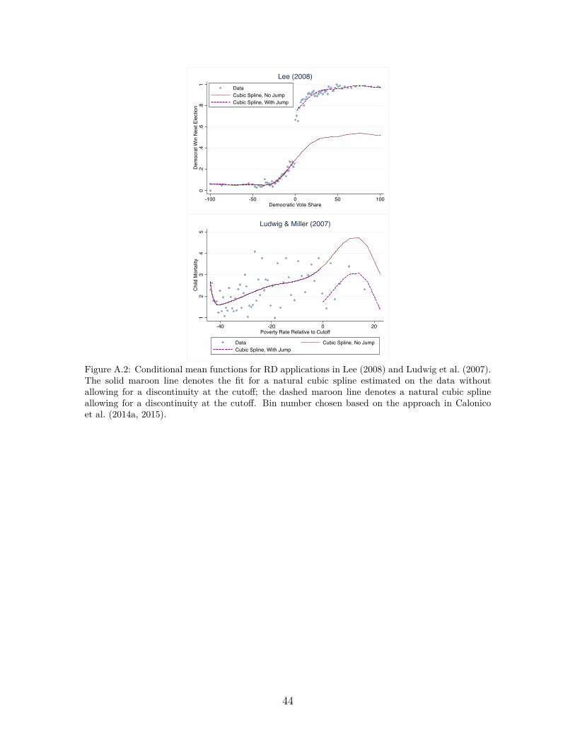
0.2

.4.6

.81

Dem

ocra

t Win

Nex

t Ele

ctio

n-100 -50 0 50 100

Democratic Vote Share

DataCubic Spline, No JumpCubic Spline, With Jump

Lee (2008)

12

34

5C

hild

Mor

talit

y

-40 -20 0 20Poverty Rate Relative to Cutoff

Data Cubic Spline, No JumpCubic Spline, With Jump

Ludwig & Miller (2007)

Figure A.2: Conditional mean functions for RD applications in Lee (2008) and Ludwig et al. (2007).The solid maroon line denotes the fit for a natural cubic spline estimated on the data withoutallowing for a discontinuity at the cuto�; the dashed maroon line denotes a natural cubic splineallowing for a discontinuity at the cuto�. Bin number chosen based on the approach in Calonicoet al. (2014a, 2015).

44

B Appendix: Proof of Finite Sample Size of Per-

mutation Test

Proposition: Under the Null Hypothesis of Policy Irrelevance and the Random KinkLocation assumption, there exists a test function „(v, y, k) for significance level –

that has an exact finite sample level of –.

Proof: Let K denote the number of potential kink points k drawn according to

distribution P . For any data vector (v, y), let

T

(1)(v, y) Æ T

(2)(v, y) Æ ... Æ T

(

¯

K)(v, y)

denote the kink estimates of T (v, y, k) ranked from smallest to largest.

For a given nominal level – œ (0, 1) and a two-sided test, we define the critical

values c and c as

c =5–

2 K

6

and c = K ≠5–

2 K

6

whereË

–

2

K

Èdenotes the largest integer less than or equal to –

2

K.

Let K

+(v, y) and K

≠(v, y) denote the number of values T

(j)(v, y) (j = 1, ... , K)

that are smaller than T

(c)(v, y) and greater than T

(c)(v, y), respectively, and let

K

0(v, y) be the total number of values of T

(j)(v, y) (j = 1, ... , K) equal to T

(c)(v, y)

or T

(c)(v, y).

Define

a(v, y) = –K ≠ (K+(v, y) + K

≠(v, y))K

0(v, y)

as the rejection probability in the case of a tie.

45

We can define a permutation test function „(v, y, k) that determines the proba-

bility of rejecting the null hypothesis given a test statistic T (v, y, k):

„(v, y, k) =

Y________]

________[

1 , T (v, y, k) < T

(c)(v, y) or T (v, y, k) > T

(c)(v, y)

a(v, y) , T (v, y, k) = T

(c)(v, y) or T (v, y, k) = T

(c)(v, y)

0 , T

(c)(v, y) < T (v, y, k) < T

(c)(v, y)

This implies that for any realization of (v, y), we have that:

ÿ

kœK„(v, y, k) = K

+(v, y) + K

≠(v, y) + a(v, y) · K

0(v, y) = –K.

Note that under the Null Hypothesis of Policy Irrelevance, the distribution of

(v, y) is invariant to the realized location of the kink point. This implies that the test

statistic T (v, y, k) is also invariant to the realization of the kink point k

ú, since the

test statistic only depends on the policy variable through its e�ect on the outcome.

Taking expectations of the expressions above over the distribution of the location of

kink points denoted as P , we thus have

–K = E

P

[ÿ

kœK„(v, y, k)] =

ÿ

kœKE

P

[„(v, y, k)] = KE

P

[„(v, y, k)]

Thus, it follows that E

P

[„(v, y, k)] = –, proving that the exact finite sample level

of the permutation test is –. ⌅

46

C Construction of Confidence Intervals Based on

Permutation Test

We construct confidence intervals by inverting the permutation test as described in

Rosenbaum (2002, chap. 2.6.2) and Imbens and Rubin (2015, chap. 5.7). For a set

of hypothetical e�ects, we reconstruct the data by subtracting out the hypothetical

e�ect and apply our permutation test to the transformed data, defining the confidence

interval as the set of hypothetical e�ects that are not rejected. Relative to the exist-

ing literature, which primarily uses a grid of hypothetical e�ects, we implement the

bisection method to find the end points of the confidence interval, which significantly

improves upon the computational cost of a grid search while delivering the same level

of precision.

The algorithm that we implement proceeds as follows:

1. Identify search region. To identify a search region over which a bisection search

is performed, we obtain lower and upper bounds, S and S, for hypothetical

e�ect sizes that lead to a rejection of the null hypothesis with the permutation

test when subtracted from the data. Quantitatively, we start with a search

region 10 times the size of the asymptotic confidence interval and iteratively

increase the search region by a factor of 10 until we have found lower and upper

bounds, S and S, at which the null hypothesis is rejected.

2. Perform bisection search in each half of search region. We split the search region

at the RK point estimate, S, and perform a bisection search in [S, S] and [S, S].

We illustrate the bisection search for the interval [S, S]:

(a) Perform permutation test subtracting out as hypothetical e�ect size the

mid-point, m, of [S, S]: m = 0.5 ú (S + S).

(b) Define new interval depending on result of permutation test at midpoint

47

m:

i. If the permutation test rejects at the midpoint m, continue algorithm

with interval [S, m].

ii. If the permutation test does not reject at midpoint m, continue algo-

rithm with interval [m, S].

(c) Implement step (a) and (b) with new interval calculated in (b) until the

search has converged. We define the search as having converged if two sub-

sequent midpoints are less than one tenth the magnitude of the asymptotic

confidence interval apart from one another.

3. Identify confidence interval. Report the confidence interval as the smallest and

largest non-rejected hypothetical e�ect sizes from step (2) of the algorithm.

48