Embed Size (px)
Citation preview

Department of Computer Science and Engineering CHALMERS UNIVERSITY OF TECHNOLOGY UNIVERSITY OF GOTHENBURG Gothenburg, Sweden 2017
A Petri Nets Semantics for
Privacy-Aware Data Flow Diagrams
Master’s thesis in Computer Science
MUSHFIQUR RAHMAN
MASTER’S THESIS IN COMPUTER SCIENCE
A Petri Nets Semantics
for Privacy-Aware Data Flow Diagrams
MUSHFIQUR RAHMAN
Department of Computer Science and Engineering
CHALMERS UNIVERSITY OF TECHNOLOGY
UNIVERSITY OF GOTHENBURG
Gothenburg, Sweden 2017
A Petri Nets Semantics for Privacy-Aware Data Flow Diagrams
MUSHFIQUR RAHMAN
© Mushfiqur Rahman, 2017
Department of Computer Science and Engineering
Chalmers University of Technology and University of Gothenburg
SE-4112 96 Göteborg
Sweden
Telephone +46 (0)31-772 1000
Supervisors: Raúl Pardo, Gerardo Schneider
Examiner: Wolfgang Ahrendt
Printed at Chalmers
Göteborg, Sweden 2017
iv
A Petri Nets Semantics for Privacy-Aware Data Flow Diagrams
MUSHFIQUR RAHMAN
Department of Computer Science and Engineering
Chalmers University of Technology and University of Gothenburg
Abstract
Privacy of personal data in information systems is gaining importance rapidly. Although data
flow diagrams (DFDs) are commonly used for designing information systems, they do not have
appropriate elements to address privacy of personal data. Privacy-aware data flow diagrams
(PA-DFDs) were introduced recently to tackle this issue. However, they lack the concrete
semantics to be formally verifiable. On the other hand, Petri net is a well-known mathematical
modeling language that has all the necessary supporting elements for formal verification. In
this work, we present appropriate transformations for PA-DFDs to Petri nets and therefore,
provide a Petri nets semantics for them. Firstly, we clearly identify different elements of PA-
DFDs. Then, we take a modular approach where for each element of PA-DFDs we present an
algorithm which transforms that element to a Petri nets representation. Secondly, we
demonstrate the effectiveness of the transformations on a case study, where we transform a
PA-DFD to a corresponding Petri nets model. The case study is quite elaborate and covers most
of the important aspects of PA-DFDs. Finally, we perform verification tasks on the obtained
Petri nets model from the case study where we check privacy properties such as purpose
limitation and accountability of the data controller. The Petri nets semantics along with the rest
of the supporting work constitute a step forward when it comes to privacy of personal data in
an information system.
Keywords: privacy policy, verification, privacy by design, data flow diagrams, privacy-aware
data flow diagrams, Petri nets

v
Acknowledgements
Firstly, I express my sincere gratitude to the Almighty for all the blessings He has been
showering me with throughout my life and pray for the same in future.
I am grateful to my parents, Munsur Ahmed and Kamrun Nahar for their unwavering support
and inspiration in every single step of my life.
I would like to sincerely thank my supervisors Raúl Pardo and Gerardo Schneider as well as
my examiner Wolfgang Ahrendt for their invaluable guidance and ineffable support throughout
the whole thesis work.
I want to mention my best friend, Obonti who has been there for me through thick and thin
while motivating me all the while.
Finally, my cordial appreciation goes to University of Gothenburg and Swedish Council for
Higher Education for awarding me with “The University of Gothenburg Study Scholarship”
without which it would have been quite difficult for me to finish my studies in Sweden.

vi
vii
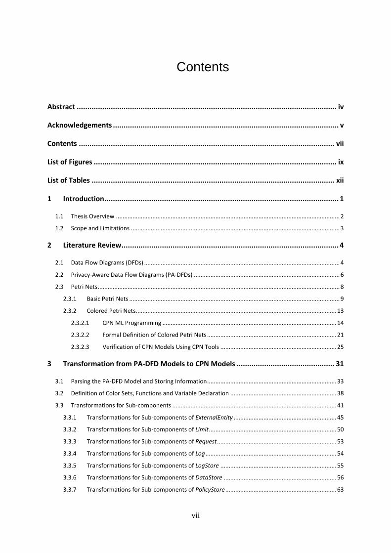
Contents
Abstract .......................................................................................................................... iv
Acknowledgements .......................................................................................................... v
Contents ........................................................................................................................ vii
List of Figures .................................................................................................................. ix
List of Tables .................................................................................................................. xii
1 Introduction .............................................................................................................. 1
1.1 Thesis Overview ....................................................................................................................................... 2
1.2 Scope and Limitations .............................................................................................................................. 3
2 Literature Review ...................................................................................................... 4
2.1 Data Flow Diagrams (DFDs) ...................................................................................................................... 4
2.2 Privacy-Aware Data Flow Diagrams (PA-DFDs) ........................................................................................ 6
2.3 Petri Nets .................................................................................................................................................. 8
2.3.1 Basic Petri Nets ............................................................................................................................... 9
2.3.2 Colored Petri Nets ......................................................................................................................... 13
2.3.2.1 CPN ML Programming ......................................................................................................... 14
2.3.2.2 Formal Definition of Colored Petri Nets .............................................................................. 21
2.3.2.3 Verification of CPN Models Using CPN Tools ...................................................................... 25
3 Transformation from PA-DFD Models to CPN Models .............................................. 31
3.1 Parsing the PA-DFD Model and Storing Information .............................................................................. 33
3.2 Definition of Color Sets, Functions and Variable Declaration ................................................................ 38
3.3 Transformations for Sub-components ................................................................................................... 41
3.3.1 Transformations for Sub-components of ExternalEntity .............................................................. 45
3.3.2 Transformations for Sub-components of Limit ............................................................................. 50
3.3.3 Transformations for Sub-components of Request ........................................................................ 53
3.3.4 Transformations for Sub-components of Log ............................................................................... 54
3.3.5 Transformations for Sub-components of LogStore ...................................................................... 55
3.3.6 Transformations for Sub-components of DataStore .................................................................... 56
3.3.7 Transformations for Sub-components of PolicyStore ................................................................... 63
viii
3.3.8 Transformations for Sub-components of Process and Reason ..................................................... 67
3.3.9 Transformations for Sub-components of Clean ............................................................................ 72
3.4 Transformations for Flows ..................................................................................................................... 72
4 Applying the Transformation on a Case Study .......................................................... 78
4.1 DFD Model for the Case Study ............................................................................................................... 78
4.2 PA-DFD Model for the Case Study .......................................................................................................... 79
4.3 CPN Model for the Case Study ............................................................................................................... 82
5 Verification on the Obtained CPN Model from the Case Study ................................. 91
6 Discussion ............................................................................................................. 101
6.1 Future Work ......................................................................................................................................... 103
7 Conclusion ............................................................................................................ 105
References ................................................................................................................... 107
ix
List of Figures
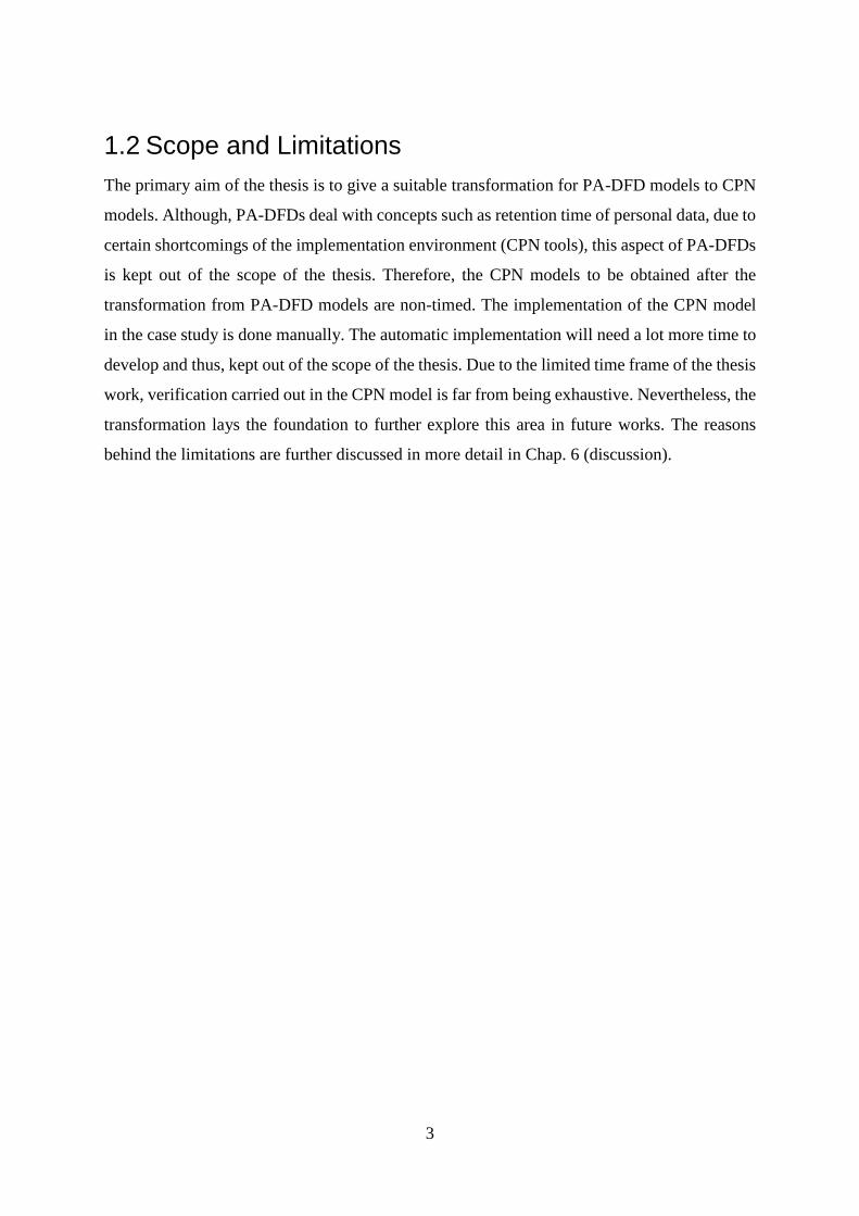
Figure 2.1: Standard symbols of DFD components with the extension ‘data deletion’ .......... 4
Figure 2.2: A simple DFD for an ATM system. ....................................................................... 5
Figure 2.3: Hotspots of a DFD and their corresponding privacy-aware transformations ........ 7
Figure 2.4: Elements of Petri nets ............................................................................................. 9
Figure 2.5: A simple Petri net ................................................................................................. 10
Figure 2.6: Petri net from Fig. 2.5 after firing transition t1 ..................................................... 12
Figure 2.7: Petri net from Fig. 2.5 after firing transition t2 ..................................................... 12
Figure 2.8: Petri net from Fig. 2.5 after firing transition t3 ..................................................... 13
Figure 2.9: Initialization of tokens in places of a CPN model ................................................ 17
Figure 2.10: A simple CPN model for ATM Machine designed in CPN Tools ..................... 19
Figure 2.11: Final marking of the CPN model from Fig. 2.10 ............................................... 20
Figure 2.12: Simple CPN example for integer sum ................................................................ 25
Figure 2.13: State space graph without markings ................................................................... 26
Figure 2.14: State space graph with markings ........................................................................ 26
Figure 2.15: Screenshot of CPN tools and some of its options .............................................. 27
Figure 2.16: Changing some options for calculating state space of a CPN model ................. 29
Figure 3.1: Different components of PA-DFDs ...................................................................... 31
Figure 3.2: Different kinds of flows in PA-DFDs .................................................................. 32
Figure 3.3: Identifying PA-DFD components and flows ........................................................ 34
Figure 3.4: Example of the general concept behind the transformation ................................. 42
Figure 3.5: An example transformation for sub-component "EE" ......................................... 49
Figure 3.6: An example transformation for sub-component "LimG" ..................................... 52
Figure 3.7: An example transformation for sub-component "DSG" ...................................... 59
Figure 3.8: An example transformation for sub-component "DSE" ....................................... 63
Figure 3.9: An example transformation for sub-component "PS" .......................................... 67
Figure 4.1: A DFD model for healthcare information system ................................................ 78
Figure 4.2: DFD and PA-DFD versions of the Process "Provide Symptoms" ...................... 80
Figure 4.3: DFD and PA-DFD versions of the DataStore "Patient History" ....................... 81
Figure 4.4: A Snippet from the CPN model corresponding Process "provide symptoms". ... 89
Figure 4.5: Snippet from the CPN model corresponding DataStore "patient history". ......... 90

x
Figure 5.1: State space queries for the model when it is initialized with token 𝑡1 only. ....... 95
Figure 5.2: State space queries for the model when it is initialized with token 𝑡2 only. ....... 96
Figure 5.3: State space queries for the model when it is initialized with token 𝑡4 only. ....... 97
Figure 5.4: State space queries for the model when it is initialized with token 𝑡5 only. ....... 98
Figure 5.5: State space queries for the model when it is initialized with token 𝑡3 along with
another token for erasure. ........................................................................................................ 99

xi

xii
List of Tables
Table 4.1: Personal data flow classification for the DFD model in Fig. 4.1........................... 80
Table 4.2: ComponentTable for storing information about each uniquely identified
components in the PA-DFD model. ......................................................................................... 82
Table 4.3: FlowTable for storing information about each flow in the PA-DFD model. ....... 84
Table 4.4: TransTable for storing information regarding transitions. ................................... 86
Table 5.1: Privacy properties applied to each hotspot ............................................................ 91

xiii
1
1 Introduction
Human beings consider privacy as an important aspect of their day-to-day life. As new systems
gather more and more information from its users, the importance of privacy of the users’
personal data is also increasing rapidly. Research awareness of privacy engineering has also
improved significantly after 2012 implying its value in modern information systems [34].
Although these research introduced many sophisticated privacy solutions, their integration with
everyday engineering practice has been slow thus far. As a result, recent history shows lots of
concerning reports related to privacy violations of various kinds. For instance, Facebook app
allowing the sharing of users’ friend networks with advertisers, Snapchat’s violation of user
expectation by not deleting users’ messages, and NoScript’s (Firefox extension) defaults
leading to de-anonymization attacks on Tor users are some of the notable examples worth
mentioning [34].
In general practice, privacy was (and still is) more of an afterthought when it came to designing
a system. However, the concept of Privacy by Design (PbD) is gaining importance and needs
to be addressed with utmost gravity. It is an approach to systems engineering which takes
privacy into account from the earliest of stages of designing a system and throughout the whole
engineering process. This will be required by the next coming European General Data
Protection Regulation (GDPR1). However, taking privacy into account while designing
information systems is not a straightforward task for software architects. They are far from
being an expert in this area. It is a common practice while designing software architectures to
use modeling languages which are based on graphical representations of the system such as
graphs or diagrams (e.g., UML) ([26], [13], [9]).
One of the most common approaches to design information systems is using Data Flow
Diagrams (or DFDs). It is an approach to model the flow of data in an information system. Due
to the way DFDs are defined, there is no room to take privacy into account when designing an
information system. A privacy-enhancing transformation ([3], [4]) of DFDs has been proposed
to tackle this issue by introducing some new and useful annotations, which ensures a certain
amount of privacy for personal data.
1 http://eur-lex.europa.eu/legal-content/en/ALL/?uri=CELEX:32016R0679
2
Although Privacy-Aware DFDs (PA-DFDs) are a promising step towards preserving the
privacy of users’ personal data, they lack concrete semantics. This makes it difficult to verify
the intended usefulness of them. Formal verification is an appropriate approach to gain
confidence in a model’s intended behavior. If formal verification is possible for PA-DFDs, it
can be used to formally guarantee and check that no privacy violation occurs.
Unfortunately, the proposed PA-DFDs cannot be used for formal verification or reasoning. A
more precise model is required to be formulated in order to perform verification regarding
privacy-related properties. One such model is Petri nets (PN) ([5], [6]). A number of tools are
also available to perform verification in a PN model. Transforming PA-DFD models into
meaningful and correct PN models in order to perform verification is one step closer to the
right direction when it comes to putting privacy in the forefront of designing information
systems.
1.1 Thesis Overview
Apart from Chap. 1 (introduction), 2 (literature review), 6 (discussion), and 7 (conclusion), the
organization of the thesis is done in three parts.
The main focus of the thesis is to give a suitable transformation from PA-DFD models to PN
models so that verification can be carried out. In order to do that, we needed to decide upon a
variant of Petri nets first. The Colored Petri Nets (CPN) [6] is chosen for this purpose. In Chap.
3, we present the transformation in a detailed manner. For each component of PA-DFDs, a
corresponding CPN transformation is given. CPN are formally introduced in Chap. 2.
Furthermore, it is essential to decide upon a tool where a CPN model can be implemented.
CPN Tools [32] is chosen to carry out this task. In Chap. 4, a case study is conducted. An
example DFD model is presented and according to the transformation proposed in [4], it is
transformed into a PA-DFD model. Afterward, according to the transformation presented in
Chap. 3, the PA-DFD model is transformed into a CPN model, which is implemented manually
in CPN Tools. The transformation for the case study is presented in detail in Chap. 4.
Finally, in Chap. 5, verification is done for the CPN model obtained from the case study by
checking some privacy related properties. The essential know-hows for verification in CPN
Tools such as state space calculation, state space queries and functions, etc. ([6], [32], [33]) are
discussed beforehand in the literature review (Chap. 2).
3
1.2 Scope and Limitations
The primary aim of the thesis is to give a suitable transformation for PA-DFD models to CPN
models. Although, PA-DFDs deal with concepts such as retention time of personal data, due to
certain shortcomings of the implementation environment (CPN tools), this aspect of PA-DFDs
is kept out of the scope of the thesis. Therefore, the CPN models to be obtained after the
transformation from PA-DFD models are non-timed. The implementation of the CPN model
in the case study is done manually. The automatic implementation will need a lot more time to
develop and thus, kept out of the scope of the thesis. Due to the limited time frame of the thesis
work, verification carried out in the CPN model is far from being exhaustive. Nevertheless, the
transformation lays the foundation to further explore this area in future works. The reasons
behind the limitations are further discussed in more detail in Chap. 6 (discussion).
4
2 Literature Review
In order to carry out the thesis work, knowledge in DFDs, PA-DFDs and Petri nets are
essentials. Therefore, we consider these in section 2.1, 2.2 and 2.3. Furthermore, in section 2.3,
we go deeper into the topic of Petri nets, introducing different variants of it, as well as
familiarizing with certain tools and their use in verification.
2.1 Data Flow Diagrams (DFDs)
System development life cycle (SDLC) is a process used for development of software system
starting from planning to the implementation phase. SDLC mainly consists of four phases,
which are analysis, design, implementation, and testing [2]. Data flow diagrams (DFDs) are
usually used during the analysis phase to produce the process model [1]. The process model
plays an important role defining the requirements in a graphical view, which makes its
reliability a key factor for improving the performance of the following phases in SDLC [2].
Figure 2.1: Standard symbols of DFD components with the extension ‘data deletion’ [4].
DFDs are graphical notations used to design how data flows in an information system. DFDs
are simple to understand. There are four basic components in a DFD: external entity (user or
an outside system that sends or receives data), process (it can be any action or computation that
modifies the data), data store (which is a database like entity for storing data) and data flow (a
route that carries data from and to the other components). Complex process is another
component representing a complex functionality or computation that is detailed in an additional
DFD [4]. It can be refined into a sub-process [3]. In [4], an extension to the standard DFDs was
proposed. The extension is another type of flow, which is called data deletion. This acts as an
5
incoming flow to data stores. This incoming flow carries the reference of the data that is stored
in the data store so that the data can be deleted from it using the reference to it. The standard
graphical symbols of DFD components, as well as the extension, are presented in Fig. 2.1.
DFDs are created with the composition of the aforementioned symbols and should obey a set
of rules in order to be well-formed and consistent [35]:
Each process should have no less than one incoming data flow and one outgoing data
flow.
All processes should have unique names.
Each data store should have at least one input data flow and one output data flow.
Two different data stores cannot be directly connected to each other with a data flow.
Two different external entities also cannot be directly connected to each other with a
data flow.
Data cannot directly move from a data store (or external entity) to an external entity (or
data store). There should be a process between the data store (external entity) and the
external entity (data store). The data should flow from the data store (external entity)
through the process to the external entity (data store).
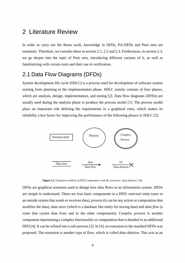
Figure 2.2: A simple DFD for an ATM system.
In Fig. 2.2, a simple DFD of an ATM (Automated Teller Machine) system is presented. It has
one external entity named “User”, three processes named “Log in to system”, “See Account
6
Information”, and “Withdraw Money”, and a data store named “Account Database”. A “User”
can log in to the system by giving his credentials and get confirmation for the login. They can
make a request to the process “See Account Information” and the process will provide the
“User” with the information after getting it from the data store “Account Database”. They can
also withdraw money by means of providing the process “Withdraw Money” with the amount
he wants to withdraw and the process will communicate with the data store to provide the
“User” with the money. Here, credentials, confirmation, request, information, amount, and
money are the flow of data inside the system.
In summary, the user can log in to the ATM system, check account information and withdraw
money from their account.
2.2 Privacy-Aware Data Flow Diagrams (PA-DFDs)
Most of the data flows in DFDs may carry personal data. This is when the privacy of personal
data comes into consideration. However, DFDs do not have necessary elements to tackle issues
regarding privacy of personal data. This is one of the primary reasons for proposing an
extension of the standard DFDs with privacy-aware annotations so that software designers can
take privacy principles into account. A DFD of such kind with privacy-aware annotations is
named Privacy-Aware DFD (PA-DFD), the outline of which was introduced in [3]. In a later
work [4], the approach of designing PA-DFDs was stated in detail.
In order to enrich a standard DFD with privacy-aware annotations, first, the designer of the
DFD needs to provide a classification of the data flows where it mentions whether a data flow
is personal or non-personal. The designer of the model provides the following additional
information for each personal data flow [4]: (i) name of external entity the data belongs to, (ii)
the purpose for the data to flow (which will be checked against the consents of the user), and
(iii) the retention time (or expiration time) for the personal data. This slightest level of
annotation on top of the standard DFD is needed to detect parts in the model (also called
hotspots [4]) which are impacted by privacy principles (in this case the European GDPR). The
next task is to transform these identified hotspots with privacy-aware annotations to obtain a
PA-DFD.
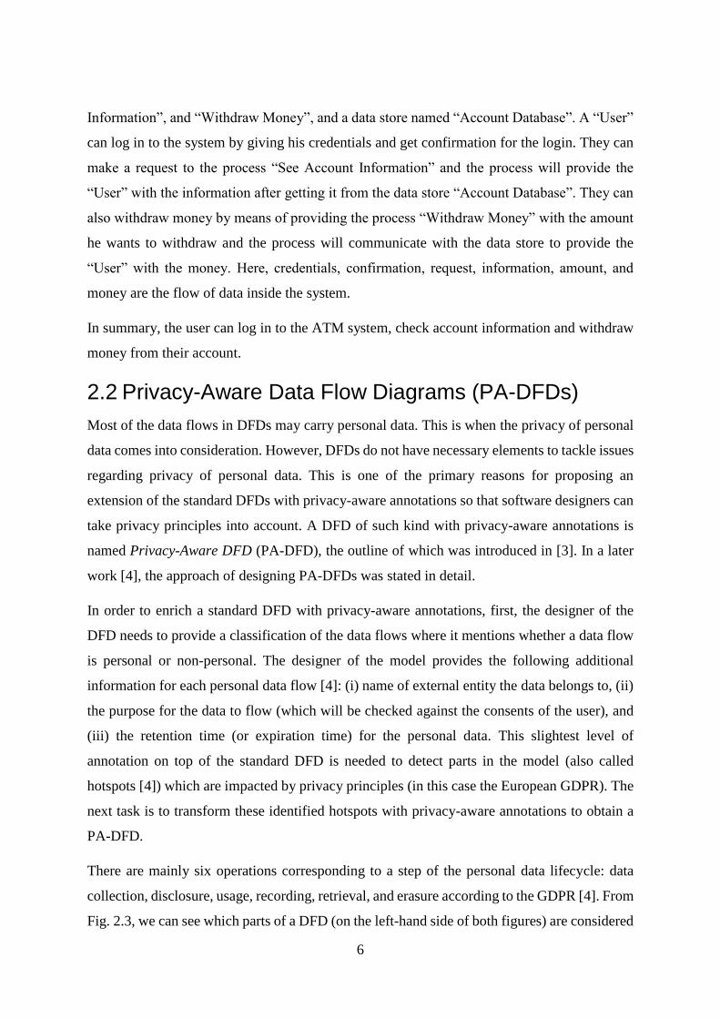
There are mainly six operations corresponding to a step of the personal data lifecycle: data
collection, disclosure, usage, recording, retrieval, and erasure according to the GDPR [4]. From
Fig. 2.3, we can see which parts of a DFD (on the left-hand side of both figures) are considered
7
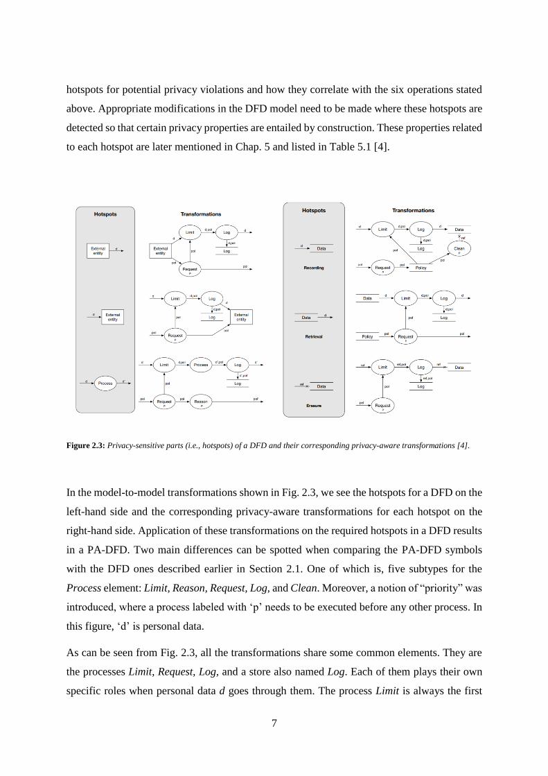
hotspots for potential privacy violations and how they correlate with the six operations stated
above. Appropriate modifications in the DFD model need to be made where these hotspots are
detected so that certain privacy properties are entailed by construction. These properties related
to each hotspot are later mentioned in Chap. 5 and listed in Table 5.1 [4].
Figure 2.3: Privacy-sensitive parts (i.e., hotspots) of a DFD and their corresponding privacy-aware transformations [4].
In the model-to-model transformations shown in Fig. 2.3, we see the hotspots for a DFD on the
left-hand side and the corresponding privacy-aware transformations for each hotspot on the
right-hand side. Application of these transformations on the required hotspots in a DFD results
in a PA-DFD. Two main differences can be spotted when comparing the PA-DFD symbols
with the DFD ones described earlier in Section 2.1. One of which is, five subtypes for the
Process element: Limit, Reason, Request, Log, and Clean. Moreover, a notion of “priority” was
introduced, where a process labeled with ‘p’ needs to be executed before any other process. In
this figure, ‘d’ is personal data.
As can be seen from Fig. 2.3, all the transformations share some common elements. They are
the processes Limit, Request, Log, and a store also named Log. Each of them plays their own
specific roles when personal data d goes through them. The process Limit is always the first
8
step for d to go through. The task of Limit is to restrict the processing of d in accordance with
the consent given for it in a policy pol. This pol needs to be provided earlier by another process
Request in order for the process Limit to perform the restriction on the processing of d later. In
addition to these two processes, Log is another common element of all the transformations. Its
only task is to perform a log operation and store a trace of the data processing on d in
accordance with its pol to a Log store. Then, it just forwards d on a data flow to the rest of the
model [4].
Transformations stated in Fig. 2.3 are different from each other and perform different tasks on
the personal data according to the consent of the external entity. In a collection we see personal
data d and the policy (which includes the consents) pol corresponding to it being received from
an External entity. Then it goes through the common elements and is forwarded to the rest of
the model. A disclosure can be said to be the opposite of a collection, where it takes both
personal data d along with its corresponding policy pol and forwards it to an External entity. A
usage similarly takes personal data d along with its corresponding policy pol and applies the
process named Process on d to get a computed data d’, which is then forwarded to the rest of
the model. On the other hand, the process Reason also forwards a changed policy pol’ which
corresponds to d’ to the rest of the model. Recording takes personal data d and its policy pol
and stores them respectively in a Data store and a Policy store. Moreover, process Clean, which
ensures the erasure of d (which has a reference ref) from the Data store if and when the policy
pol corresponding to it conforms to it. Typically d is erased when its retention time expires or
a consent in its policy pol that indicates to its erasure. A retrieval takes personal data d and its
policy pol respectively from a Data store and a Policy store and forwards them to the rest of
the model after using the common elements on them. Lastly, an erasure takes a reference ref
and the policy pol which is related to the referenced data. It then performs the erasure of said
data from the Data store.
2.3 Petri Nets
Petri nets [5] are considered a powerful modeling formalisms not only in computer science but
also in system engineering and many other disciplines [6]. The theoretical part of Petri nets
makes it possible to do precise modeling and analysis of system behavior. On the other hand,
the graphical representation of Petri nets helps visualize the state changes of a modeled system
[6]. Petri nets have been used to model really complex and dynamic event-driven systems.
9
Important examples of such include, manufacturing plants ([7],[8],[6]), command and control
systems [10], computers networks [11], workflows [12], logistic networks [14], real-time
computing systems ([15], [16]), and communication systems [17].
There exists a number of different variants of Petri nets. There are mainly two kinds of Petri
nets: low-level (basic) and high-level. The Petri nets relevant to this thesis are explained with
their formal definitions in the following sections of this chapter, starting with the low-level or
basic one.
2.3.1 Basic Petri Nets
A Petri net is a bipartite graph and consists of just three types of basic elements. These are
places, transitions, and arcs. This graph has two types of nodes. A place is represented as a
circle; a transition is represented as a bar or box. Arcs can directly connect places to transitions
as well as transitions to places, but not transitions to transitions or places to places. A token is
another primitive concept of a Petri net. Tokens are represented as black dots residing inside
places of a Petri net graph. Tokens can be present or absent in certain places, which, for
instance, can indicate whether conditions associated with those places are true or false [6].
Elements for Petri nets graphical representation can be seen in Fig. 2.4.
Figure 2.4: Elements of Petri nets.
Definition 1. A Petri net is formally defined [6] as a five-tuple 𝑁 = (𝑃, 𝑇, 𝐼, 𝑂,𝑀0)1, where
i. 𝑃 = {𝑝1, 𝑝2, … , 𝑝𝑚} is a finite set of places;
ii. 𝑇 = {𝑡1, 𝑡2, … , 𝑡𝑛} is a finite set of transitions, 𝑃 ∪ 𝑇 ≠ ∅, and 𝑃 ∩ 𝑇 = ∅;
iii. 𝐼: 𝑃 × 𝑇 → 𝑁 is an input function which defines directed arcs connecting places to
transitions. Here, 𝑁 is a set of nonnegative integers;
iv. 𝑂: 𝑇 × 𝑃 → 𝑁 is an output function defining directed arcs from transitions to places;
v. 𝑀0: 𝑃 → 𝑁 is the initial marking.
1 We will be using ′ = ′ for assignment, ′ ≡ ′ for equality, and ′ ≠ ′ for inequality throughout the document.
place transition arc token
10
As stated earlier, arcs directly connect places to transitions or transitions to places. Assume,
there is a place 𝑝𝑗 and a transition 𝑡𝑖. If there is an arc directed from 𝑝𝑗 to 𝑡𝑖, according to Def.
1, 𝑝𝑗 is an input place of 𝑡𝑖, and is denoted by 𝐼(𝑝𝑗, 𝑡𝑖) = 1. On the other hand, if there is an
arc directed from 𝑡𝑖 to 𝑝𝑗, according to Def. 1, 𝑝𝑗 is an output place of 𝑡𝑖, and is denoted by
𝑂(𝑡𝑖, 𝑝𝑗) = 1. If 𝐼(𝑝𝑗 , 𝑡𝑖) = 𝑘 (or 𝑂(𝑡𝑖, 𝑝𝑗) = 𝑘), it means there exist 𝑘 arcs connecting 𝑝𝑗 to
𝑡𝑖 (or 𝑡𝑖 to 𝑝𝑗) in parallel. However, in the graphical representation, parallel arcs connecting a
place (transition) to a transition (place) are usually represented by a single directed arc with the
multiplicity or weight of 𝑘.
A marking of a Petri net is represented by the distribution of tokens over places. A Petri net
has an initial marking which assigns a nonnegative integer to each place. Marking changes
depending on the execution of Petri nets and movement of tokens from one place to another. It
is also referred to as change of state.
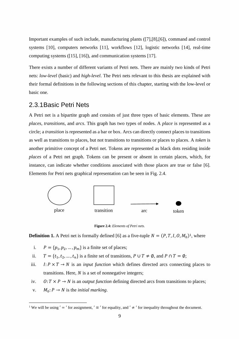
Figure 2.5: A simple Petri net.
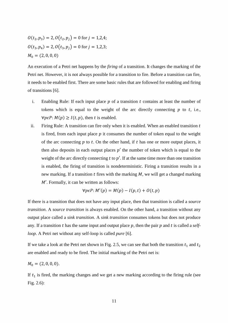
Fig. 2.5 shows an example of a simple Petri net, from where we have the following information:
𝑃 = {𝑝1, 𝑝2, 𝑝3, 𝑝4}
𝑇 = {𝑡1, 𝑡2, 𝑡3}
𝐼(𝑝1, 𝑡1) = 1, 𝐼(𝑝1, 𝑡2) = 1, 𝐼(𝑝1, 𝑡𝑖) = 0 for 𝑖 = 3;
𝐼(𝑝2, 𝑡3) = 1, 𝐼(𝑝2, 𝑡𝑖) = 0 for 𝑖 = 1, 2;
𝐼(𝑝3, 𝑡3) = 1, 𝐼(𝑝3, 𝑡𝑖) = 0 for 𝑖 = 1, 2;
𝑂(𝑡1, 𝑝2) = 2, 𝑂(𝑡1, 𝑝𝑗) = 0 for 𝑗 = 1,3,4;
2
p1
p2
p3
p4
t2
t1
t3
11
𝑂(𝑡2, 𝑝3) = 2, 𝑂(𝑡2, 𝑝𝑗) = 0 for 𝑗 = 1,2,4;
𝑂(𝑡3, 𝑝4) = 2, 𝑂(𝑡3, 𝑝𝑗) = 0 for 𝑗 = 1,2,3;
𝑀0 = (2, 0, 0, 0)
An execution of a Petri net happens by the firing of a transition. It changes the marking of the
Petri net. However, it is not always possible for a transition to fire. Before a transition can fire,
it needs to be enabled first. There are some basic rules that are followed for enabling and firing
of transitions [6].
i. Enabling Rule: If each input place 𝑝 of a transition 𝑡 contains at least the number of
tokens which is equal to the weight of the arc directly connecting 𝑝 to 𝑡, i.e.,
∀𝑝𝜖𝑃: 𝑀(𝑝) ≥ 𝐼(𝑡, 𝑝), then 𝑡 is enabled.
ii. Firing Rule: A transition can fire only when it is enabled. When an enabled transition 𝑡
is fired, from each input place 𝑝 it consumes the number of token equal to the weight
of the arc connecting 𝑝 to 𝑡. On the other hand, if 𝑡 has one or more output places, it
then also deposits in each output places 𝑝′ the number of token which is equal to the
weight of the arc directly connecting 𝑡 to 𝑝′. If at the same time more than one transition
is enabled, the firing of transition is nondeterministic. Firing a transition results in a
new marking. If a transition 𝑡 fires with the marking 𝑀, we will get a changed marking
𝑀′. Formally, it can be written as follows:
∀𝑝𝜖𝑃: 𝑀′(𝑝) = 𝑀(𝑝) − 𝐼(𝑝, 𝑡) + 𝑂(𝑡, 𝑝)
If there is a transition that does not have any input place, then that transition is called a source
transition. A source transition is always enabled. On the other hand, a transition without any
output place called a sink transition. A sink transition consumes tokens but does not produce
any. If a transition 𝑡 has the same input and output place 𝑝, then the pair 𝑝 and 𝑡 is called a self-
loop. A Petri net without any self-loop is called pure [6].
If we take a look at the Petri net shown in Fig. 2.5, we can see that both the transition 𝑡1 and 𝑡2
are enabled and ready to be fired. The initial marking of the Petri net is:
𝑀0 = (2, 0, 0, 0).
If 𝑡1 is fired, the marking changes and we get a new marking according to the firing rule (see
Fig. 2.6):
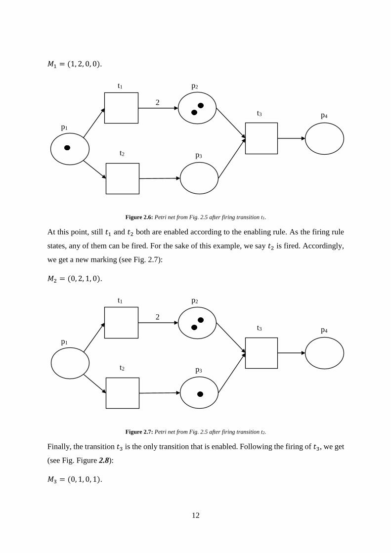
12
𝑀1 = (1, 2, 0, 0).
Figure 2.6: Petri net from Fig. 2.5 after firing transition t1.
At this point, still 𝑡1 and 𝑡2 both are enabled according to the enabling rule. As the firing rule
states, any of them can be fired. For the sake of this example, we say 𝑡2 is fired. Accordingly,
we get a new marking (see Fig. 2.7):
𝑀2 = (0, 2, 1, 0).
Figure 2.7: Petri net from Fig. 2.5 after firing transition t2.
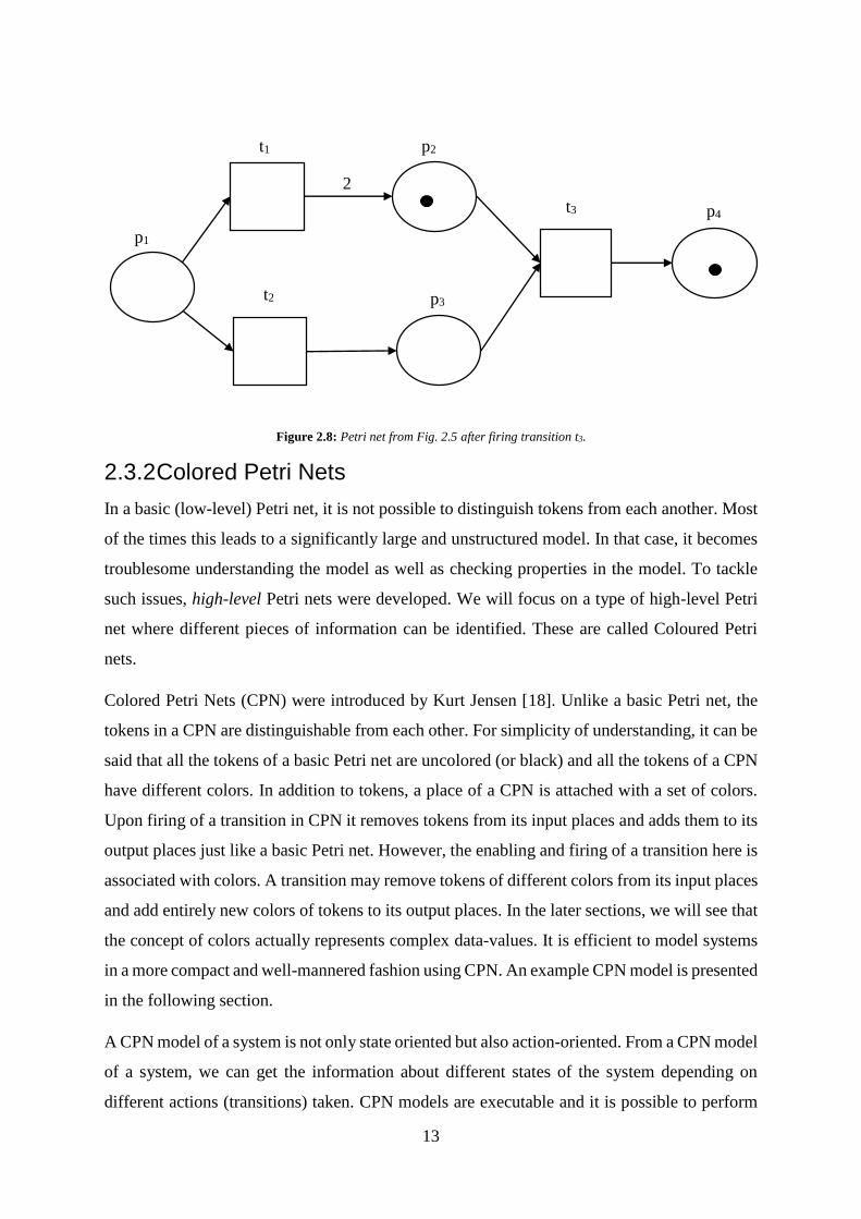
Finally, the transition 𝑡3 is the only transition that is enabled. Following the firing of 𝑡3, we get
(see Fig. Figure 2.8):
𝑀3 = (0, 1, 0, 1).
2
p1
p2
p3
p4
t2
t1
t3
2
p1
p2
p3
p4
t2
t1
t3
13
Figure 2.8: Petri net from Fig. 2.5 after firing transition t3.
2.3.2 Colored Petri Nets
In a basic (low-level) Petri net, it is not possible to distinguish tokens from each another. Most
of the times this leads to a significantly large and unstructured model. In that case, it becomes
troublesome understanding the model as well as checking properties in the model. To tackle
such issues, high-level Petri nets were developed. We will focus on a type of high-level Petri
net where different pieces of information can be identified. These are called Coloured Petri
nets.
Colored Petri Nets (CPN) were introduced by Kurt Jensen [18]. Unlike a basic Petri net, the
tokens in a CPN are distinguishable from each other. For simplicity of understanding, it can be
said that all the tokens of a basic Petri net are uncolored (or black) and all the tokens of a CPN
have different colors. In addition to tokens, a place of a CPN is attached with a set of colors.
Upon firing of a transition in CPN it removes tokens from its input places and adds them to its
output places just like a basic Petri net. However, the enabling and firing of a transition here is
associated with colors. A transition may remove tokens of different colors from its input places
and add entirely new colors of tokens to its output places. In the later sections, we will see that
the concept of colors actually represents complex data-values. It is efficient to model systems
in a more compact and well-mannered fashion using CPN. An example CPN model is presented
in the following section.
A CPN model of a system is not only state oriented but also action-oriented. From a CPN model
of a system, we can get the information about different states of the system depending on
different actions (transitions) taken. CPN models are executable and it is possible to perform
2
p1
p2
p3
p4
t2
t1
t3
14
simulations of the model of a system to learn about different states and behaviors of the system
[21].
CPN is considered a discrete-event modeling language. It has been under development since
1979 by the CPN group at Aarhus University, Denmark. Along with the characteristics of basic
Petri nets, it possesses the power of a high-level programming language. The CPN ML
programming language is based on the functional programming language Standard ML ([19],
[20]). Like functional programming, CPN ML provides primitives for defining data types and
data manipulation, which in turn help models to be compact [21]. There are quite a lot of
modeling languages [22] developed for concurrent and distributed systems and CPN is one of
them. Other notable examples like such include the Calculus of Communicating Systems [23]
as supported by, for example, the Edinburgh Concurrency Workbench [24], Statecharts [25] as
supported by, for example, the VisualState tool [20], Promela [27], as supported by the SPIN
tool [28], and Timed Automata [29] as supported by, for example, the UPPAAL tool [30]. The
CPN group at Aarhus University, Denmark has developed industrial-strength tools like
Design/CPN [31] and CPN Tools [32], which support CPN. In this thesis, we chose to work
with CPN Tools to create and simulate CPN models as well as checking certain properties in
them.
2.3.2.1 CPN ML Programming
Before presenting the formal specification of CPNs in section 2.3.2.2, in this section, we take
an introductory look at how to use CPN ML programming language (to define color sets and
functions, declare variables, and write inscriptions) when creating a CPN model. This will help
understand the formal specification of CPNs, as we will be illustrating that with the help of an
example model where this programming language is used. We will not cover every aspect of
CPN ML in this section as it is an enormous topic to explain. We are only focusing on parts of
CPN ML essential to support the understanding of the thesis work done. The reader is referred
to [21] where the CPN ML programming language is discussed in a more detailed manner.
There are some predefined set of basic types in CPN ML, which are inherited from Standard
ML (SML). The basic types are as follows:
Basic types:
o int (the set of integers)
o string (the set of all text strings)
15
o bool (has two values, true and false)
o real (the set of all real numbers)
o unit (has only one value, written (). It is used to represent uncolored tokens.)
A color set is a type, which is defined using a color set declaration colset …=…. Basic types
are used to define simple color sets. Simple color sets can then be used further to create
structured color sets using a set of color set constructors such as, with, product,
record, list [21]. When a color set is declared, it can later be used to type places in a
CPN model. Furthermore, the color set constructor with can be used to define sub color sets
or entirely new color sets. Some examples:
Defining simple color sets:
o colset I = int;
o colset S = string;
o colset B = bool;
Defining sub color sets using with:
o colset Price = int with 0..1500; (this means Price can only
have integer values from 0 to 1500)
o colset Letter = string with “a”..”z”;
o colset BinaryBool = bool with (zero,one);
Defining new color sets using with:
o colset Sports = with Football | Cricket | Handball;
o colset SmartPhones = with Android | IPhone | Windows;
Defining new color sets using product, record and list:
o colset PhonePrice = product SmartPhones * Price;
Possible values: (Android, 1000),(IPhone, 1300), …
o colset listOfSports = list Sports;
Possible values: [Cricket],[Handfall, Football], …
o colset ItemOffer =
record item:S * regularCost:Price * discount:Price
16
Possible values: {item=”Oil”, regularCost=15, discount=3},
…
There are some basic operations on lists, records, and products. [] denotes an empty list.
Concatenation of lists can be made using the operator ^^, e.g., [5,4,3]^^[7,1,8]
evaluates to [5,4,2,7,1,8]. To add an element in front of a list, the operator :: can be
used, e.g., “n”::[“o”,”i”,”c”,”e”] evaluates to [“n”,”o”,”i”,”c”,”e”]. We
can use the operator # to extract a field of a record, e.g., #n{m=13,n=2} evaluates to 2. The
same operator can be used to extract an element from a product value, e.g.,
#3(“a”,”b”,”c”,”d”) evaluates to “c”.
Furthermore, there are some other basic operators, such as ~ (unary minus), + (addition for
reals and integers), - (subtraction for reals and integers), * (multiplication for reals and
integers), / (division for reals and integers), div (division for integers), mod (modulo for
integers), = (equal to), < (less than), > (greater than), <= (less than or equal to), >= (greater
than or equal to), <> (not equal to) and ^ (string concatenation). There are also some logical
operators available; these include not (negation), andalso (logical AND), orelse (logical
OR) and if then else (if takes a boolean argument; upon its evaluation to true, it
returns the value after then; upon its evaluation to false, it returns the value after else;
values after then and else are of the same type). The use of some of these operators are
presented with the following examples:
not(1>2) andalso (1=1 orelse 2<1)
value: true.
If 2<>2 then “hi” else “hi”^” “^”there”
Value: “hi there”
We also declare variable and constants. To declare a variable, the keyword var is used. On
the other hand, the keyword val is used to declare a constant. Examples of variable and
constant declarations are as follows:
var a:Price;
val b = 1132;
17
Now, we turn our attention to some of the important aspects of CPN ML programming
language which deal with the graphical representation of the CPN model. The first thing that
comes to mind when talking about any kind of Petri net model, is the number of tokens and
their availability in different places in the model. A place can either be empty or non-empty
with one or more tokens. In order to initialize places with multiple tokens, we need multisets
[21]. Multisets in CPN are denoted using this notation: a1`v1++a2`v2++…++an`vn where
v1 represents one of the elements and a1 represents the number of times it occurs in the
multiset. Another important thing to keep in mind while initializing tokens in a place is that the
type or color set of that place needs to be the same as the tokens’. We can look at the examples
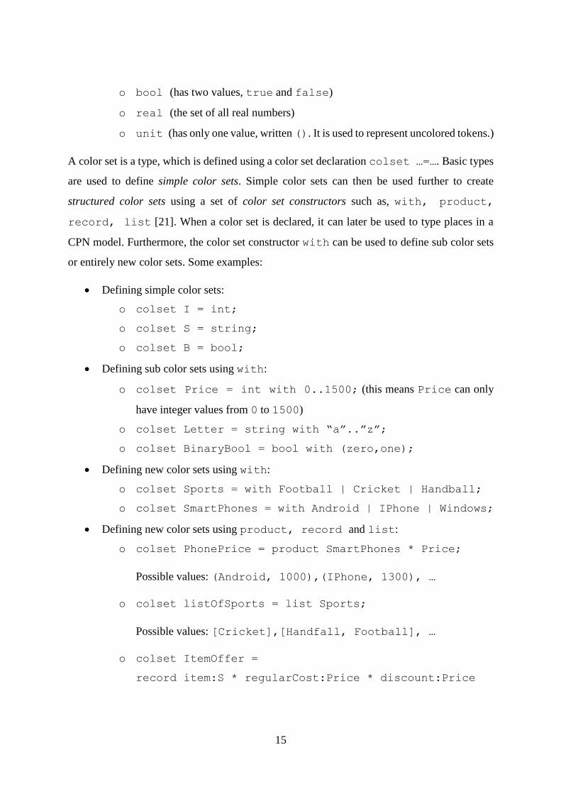
given in Fig. 2.9 to get a clear idea of how tokens are initialized in a place of a CPN model.
The place p1 is empty. On the other hand, the place p2 has only one token with an integer
value of 1 and p3 has 9 tokens. In CPN, multisets are implemented as lists, e.g.,
3`7++2`5++4`1 is equivalent to [7,7,7,5,5,1,1,1,1]. Therefore, it is useful when
using list functions on multisets.
Figure 2.9: Initialization of tokens in places of a CPN model.
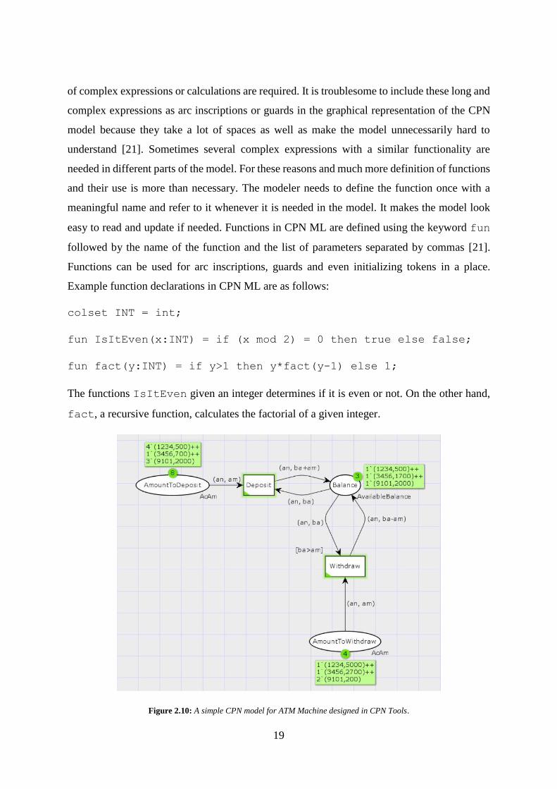
One of the most important elements of any kind of Petri net is the arc or directed arc that
connects a place to a transition and vice versa. An arc inscription plays a major role while
connecting places and transitions to each other. It essentially represents the value of a token
that goes through an arc. An inscription of an arc possesses the ability to change the value of a
token that goes through that arc before being forwarded to a place or a transition. An arc
inscription can be a variable, a constant, a multiset, a function (which we will be talking about
later in this section) or some other expressions. We can see different types of arc inscriptions
in the CPN model given in Fig. 2.10. Later in this section, there is an explanation for the model
which covers the functionalities of the different arcs used in the model.
Another concept that is necessary to get familiarized with to understand enabling and firing of
transitions in CPN, is binding. If there is a transition t and in its input and output arcs have
INT INT INT
1 3`7++2`5++4`1 p1 p2 p3

18
variables a1,a2,…,an, then a binding of t assigns a concrete value v1,v2,…,vn to each
of these variables. The assigned values should be of the same type as the variables they are
assigned to. A binding is enabled when there are tokens whose values match the values of the
variables on the input and output arcs. After necessary bindings are enabled, it can occur, i.e.,
the transition can fire, consuming and producing tokens respectively from the input and to the
output places. If an arc has a variable to which the transition cannot assign any value, then that
variable is considered unbound. The pair (transition, <bindings>) is called a
binding element. Here, for the transition t, the binding element is (t,
<a1=v1,a2=v2,…,an=vn>).
Enabling and firing of a transition also depend on the evaluation of a guard used attached to
that transition. A guard is a Boolean expression, which needs to be evaluated to true in order
for the transition to enable and fire. Only those binding elements are enabled which evaluate
the guard to true. A guard is denoted by square brackets. In the model shown in Fig. 2.10, we
see the transition withdraw has a guard [y<x], which means if the value of y is less than
the value of x, then the transition is enabled and ready to fire.
In addition to binding and guards, a transition can enable and fire depending upon the priority
attached to it. In CPN Tools there are three standard priorities given:
val P_HIGH = 100;
val P_NORMAL = 1000;
val P_LOW = 10000;
As can be seen, they are simply three constants with integer values, where lower value suggests
a higher priority. By default, all transitions in a CPN model are attached with the P_NORMAL
priority. If two transitions t1 and t2, both have all of their bindings enabled and guards
evaluated to true, but t1 is attached with the priority P_NORMAL and t2 is attached with
P_HIGH, then only t2 will be enabled and ready to be fired. Only after t2 is fired, if there are
no necessary bindings enabled for it or no guards evaluated to true, t1 will be enabled and
ready to be fired. We can declare our own priorities in CPN Tools.
Like other programming languages, CPN ML programming language also supports the
definition and use of functions. Most of the times when modeling a complex system, the use
19
of complex expressions or calculations are required. It is troublesome to include these long and
complex expressions as arc inscriptions or guards in the graphical representation of the CPN
model because they take a lot of spaces as well as make the model unnecessarily hard to
understand [21]. Sometimes several complex expressions with a similar functionality are
needed in different parts of the model. For these reasons and much more definition of functions
and their use is more than necessary. The modeler needs to define the function once with a
meaningful name and refer to it whenever it is needed in the model. It makes the model look
easy to read and update if needed. Functions in CPN ML are defined using the keyword fun
followed by the name of the function and the list of parameters separated by commas [21].
Functions can be used for arc inscriptions, guards and even initializing tokens in a place.
Example function declarations in CPN ML are as follows:
colset INT = int;
fun IsItEven(x:INT) = if (x mod 2) = 0 then true else false;
fun fact(y:INT) = if y>1 then y*fact(y-1) else 1;
The functions IsItEven given an integer determines if it is even or not. On the other hand,
fact, a recursive function, calculates the factorial of a given integer.
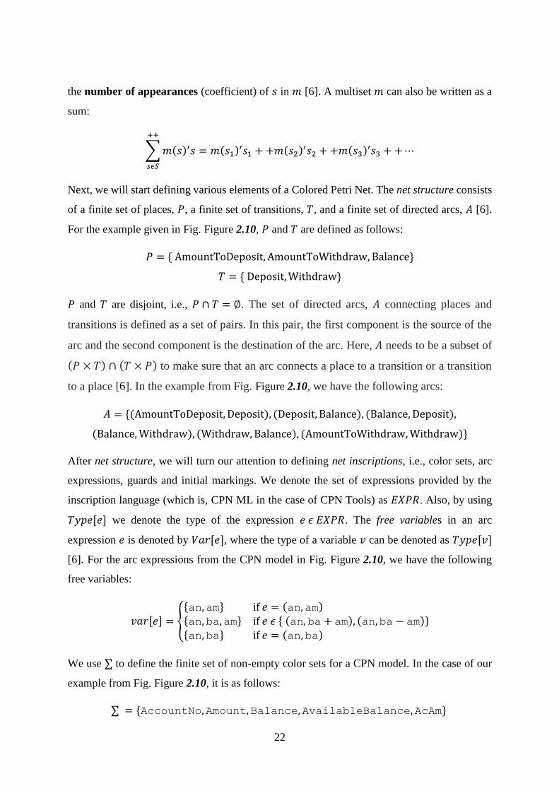
Figure 2.10: A simple CPN model for ATM Machine designed in CPN Tools.
20
We will end this section by giving a simple yet proper example of a CPN model to demonstrate
most of the aspects in CPN ML. In Fig. 2.10, we show a simple CPN model for an ATM
machine, where one can withdraw and deposit money with the identification of their account
number. For this model we need to define the following color sets and variables:
colset AccountNo = int with 1..10000;
colset Amount = int with 1..50000;
colset Balance = int;
colset AvailableBalance = product AccountNo * Balance;
colset AcAm = product AccountNo * Amount;
var an:AccountNo;
var am:Amount;
var ba:Balance;
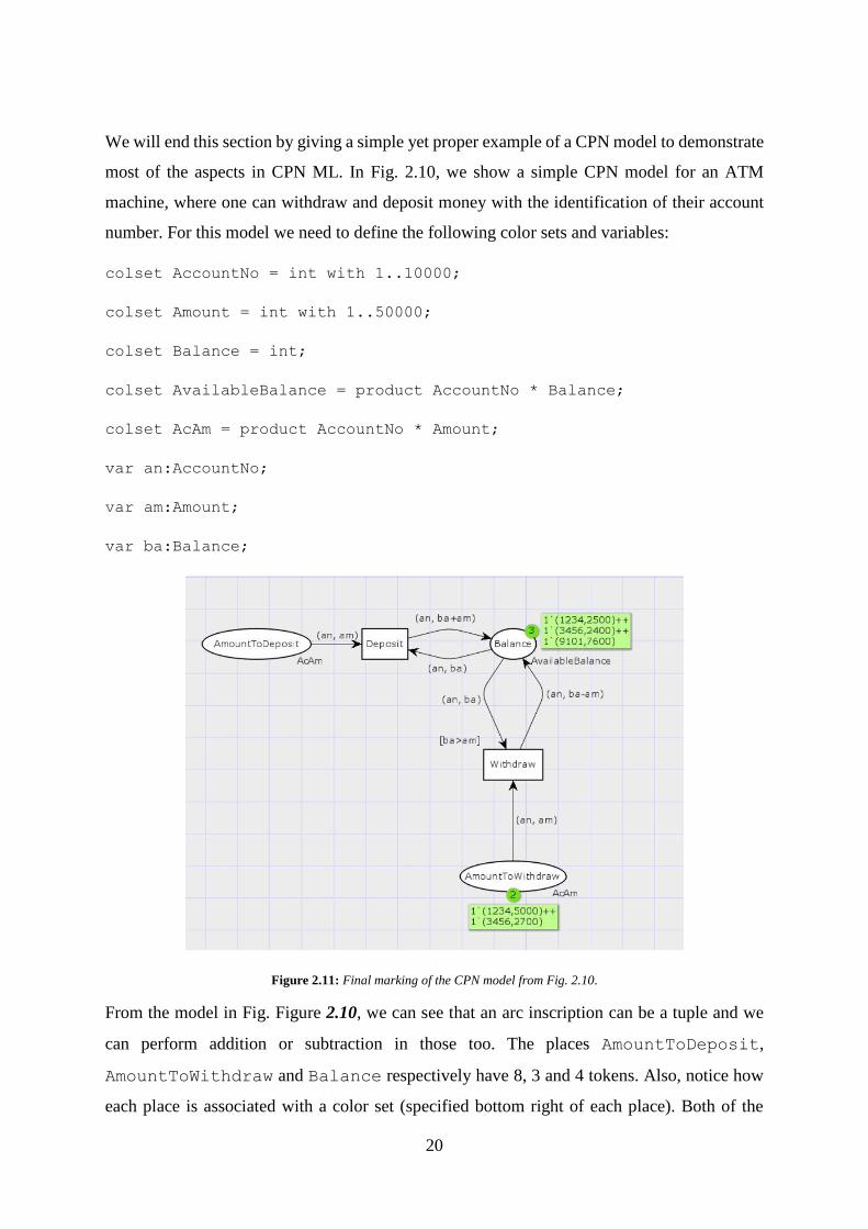
Figure 2.11: Final marking of the CPN model from Fig. 2.10.
From the model in Fig. Figure 2.10, we can see that an arc inscription can be a tuple and we
can perform addition or subtraction in those too. The places AmountToDeposit,
AmountToWithdraw and Balance respectively have 8, 3 and 4 tokens. Also, notice how
each place is associated with a color set (specified bottom right of each place). Both of the

21
transitions are enabled (CPN Tools marks the transition border with green color when it is
enabled). There is no guard attached to the transition Deposit. However, the transition
Withdraw has a guard attached to it, which is [ba>am]. It means, if the available balance
of an account is less than what is asked to be withdrawn from that account, then for that account
money cannot be withdrawn. The final marking of the model (where, no transition is enabled)
is shown in Fig. Figure 2.11.
The reason for the transition Deposit to be disabled is pretty straightforward: its input place
AmountToDeposit does not have any token left in it. On the other hand, the reason for the
transition Withdraw to be disabled is quite different. Although its input place
AmountToWithdraw has more than the necessary amount of tokens for it to be enabled, the
guard [ba>am] does not allow Withdraw to be enabled. The available balance for both the
accounts 1234 and 3456 are less (can be seen in the place Balance) than the amount
requested to be withdrawn (can be seen in the place AmountToWithdraw). Therefore, the
guard [ba>am] evaluates to false and disables the transition Withdraw.
2.3.2.2 Formal Definition of Colored Petri Nets
In section 2.3.1, we have looked at the formal definition of basic Petri nets. In this section, we
will take a look at the formal definition of Colored Petri Nets (non-hierarchical), which we will
be using for this thesis work. When presenting a definition we will use the example in Fig.
Figure 2.10 for illustration. The color sets definition, as well as the variable for the example,
are already given in the previous section.
First, we give the definition [6] of multisets, which is used in the definition for Colored Petri
Nets. Example of multisets can be the following three multisets 𝑚𝐴𝐷 , 𝑚𝐴𝑊, and 𝑚𝐵 over the
color sets AcAm and AvailableBalance corresponding to the markings of
AmountToDeposit, AmountToWithdraw, and Balance are in Fig. Figure 2.10:
𝑚𝐴𝐷 = 4’(1234,500) + +1`(3456,700) + +3`(9101,2000)
𝑚𝐴𝑊 = 1’(1234,5000) + +1`(3456,2700) + +2`(9101,200)
𝑚𝐵 = 1’(1234,500) + +1`(3456,1700) + +1`(9101,2000)
Definition 2. Assume there is a non-empty set 𝑆 = {𝑠1, 𝑠2, 𝑠3…}. A multiset over S is a
function 𝑚 ∶ 𝑆 → 𝑁 that maps each element 𝑠 𝜖 𝑆 into a non-negative integer 𝑚(𝑠) 𝜖 𝑁 called
22
the number of appearances (coefficient) of 𝑠 in 𝑚 [6]. A multiset 𝑚 can also be written as a
sum:
∑𝑚(𝑠)′𝑠 = 𝑚(𝑠1)′𝑠1 ++𝑚(𝑠2)
′𝑠2 ++𝑚(𝑠3)′𝑠3 + +⋯
++
𝑠𝜖𝑆
Next, we will start defining various elements of a Colored Petri Net. The net structure consists
of a finite set of places, 𝑃, a finite set of transitions, 𝑇, and a finite set of directed arcs, 𝐴 [6].
For the example given in Fig. Figure 2.10, 𝑃 and 𝑇 are defined as follows:
𝑃 = { AmountToDeposit, AmountToWithdraw, Balance}
𝑇 = { Deposit,Withdraw}
𝑃 and 𝑇 are disjoint, i.e., 𝑃 ∩ 𝑇 = ∅. The set of directed arcs, 𝐴 connecting places and
transitions is defined as a set of pairs. In this pair, the first component is the source of the
arc and the second component is the destination of the arc. Here, 𝐴 needs to be a subset of
(𝑃 × 𝑇) ∩ (𝑇 × 𝑃) to make sure that an arc connects a place to a transition or a transition
to a place [6]. In the example from Fig. Figure 2.10, we have the following arcs:
𝐴 = {(AmountToDeposit, Deposit), (Deposit, Balance), (Balance, Deposit),
(Balance,Withdraw), (Withdraw, Balance), (AmountToWithdraw,Withdraw)}
After net structure, we will turn our attention to defining net inscriptions, i.e., color sets, arc
expressions, guards and initial markings. We denote the set of expressions provided by the
inscription language (which is, CPN ML in the case of CPN Tools) as 𝐸𝑋𝑃𝑅. Also, by using
𝑇𝑦𝑝𝑒[𝑒] we denote the type of the expression 𝑒 𝜖 𝐸𝑋𝑃𝑅. The free variables in an arc
expression 𝑒 is denoted by 𝑉𝑎𝑟[𝑒], where the type of a variable 𝑣 can be denoted as 𝑇𝑦𝑝𝑒[𝑣]
[6]. For the arc expressions from the CPN model in Fig. Figure 2.10, we have the following
free variables:
𝑣𝑎𝑟[𝑒] = {
{an,am} if 𝑒 = (an,am){an,ba,am} if 𝑒 𝜖 { (an,ba+ am), (an,ba − am)}{an,ba} if 𝑒 = (an,ba)
We use ∑ to define the finite set of non-empty color sets for a CPN model. In the case of our
example from Fig. Figure 2.10, it is as follows:
∑ = {AccountNo,Amount,Balance,AvailableBalance,AcAm}
23
Set of variables can be denoted by 𝑉. Each variable should have a type that is in ∑. For the
CPN model in Fig. Figure 2.10, we have the following variables:
𝑉 = {an:AccountNo,am:Amount,ba:Balance}
The color set function 𝐶 ∶ 𝑃 → ∑ assigns to each place 𝑝 a color set 𝐶(𝑝), which belongs to
the set ∑. For the example model in Fig. Figure 2.10, it is defined as
𝐶(𝑝) = {AcAm if 𝑝 𝜖 {AmountToDeposit, AmountToWithdraw}
AvailableBalance if 𝑝 = Balance
There is also a guard function 𝐺: 𝑇 → 𝐸𝑋𝑃𝑅𝑉, which assigns to each transition 𝑡 𝜖 𝑇 a guard
𝐺(𝑡), which needs to be a boolean expression, i.e., 𝑇𝑦𝑝𝑒[𝐺(𝑡)] = 𝐵𝑜𝑜𝑙. Here, 𝐸𝑋𝑃𝑅𝑉 means
that there exists 𝑒 𝜖 𝐸𝑋𝑃𝑅 such that 𝑉𝑎𝑟[𝑒] ⊆ 𝑉. That means, the set of free variables
appearing in the guard expression 𝑒 is required to form a subset of 𝑉. For that reason,
𝐺(𝑡) 𝜖 𝐸𝑋𝑃𝑅𝑉. For the model in Fig. Figure 2.10, the guard expressions are as follows:
𝐺(𝑡) = {𝑏𝑎 > 𝑎𝑚 if 𝑡 = Withdraw𝑡𝑟𝑢𝑒 for all 𝑡 𝜖 𝑇 𝑤ℎ𝑒𝑟𝑒 𝑡 ≠ Withdraw
In a CPN model, when a transition does not specify a guard explicitly, that means there is an
implicit constant guard true.
There are two more functions, arc expression function and initialization function. First, we take
a look at the former one. It is defined as 𝐸: 𝐴 → 𝐸𝑋𝑃𝑅𝑉, which assigns to each arc 𝑎 𝜖 𝐴 an
expression 𝐸(𝑎). An arc expression is essentially a multiset. For example, in Fig. Figure 2.10,
the arc expression (an,am) of the arc connecting the place AmountToDeposit to the
transition Deposit can be alternatively written as 1`(an,am), which is the same thing. Here,
1` is implicit. However, if it was written as 2`(an,am), that would have meant that the arc
was carrying two identical copies of the same token. Therefore, for an arc (𝑝, 𝑡) 𝜖 𝐴, connecting
a place 𝑝 𝜖 𝑃 to a transition 𝑡 𝜖 𝑇, it should be the case that the type of the arc expression is the
multiset type over the color set 𝐶(𝑝) of the place 𝑝, i.e., 𝑇𝑦𝑝𝑒[𝐸(𝑝, 𝑡)] = 𝐶(𝑝)𝑀𝑆. Similarly,
for an arc connecting a transition 𝑡 𝜖 𝑇 to a place 𝑝 𝜖 𝑃, 𝑇𝑦𝑝𝑒[𝐸(𝑡, 𝑝)] = 𝐶(𝑝)𝑀𝑆. The arc
expression function for the example model in Fig. Figure 2.10 is given as follows:
24
𝐸(𝑎) =
{
1`(an,am )
if 𝑎 𝜖 {(AmountToDeposit, Deposit).(AmountToWithdraw,Withdraw)}
(an,ba) if 𝑎 𝜖 {(Balance, Deposit), (Balance,Withdraw)}
(an,ba+ am) if 𝑎 = (Deposit, Balance)
(an,ba− am) if 𝑎 = (Withdraw, Balance)
Finally, we have the initialization function 𝐼: 𝑃 → 𝐸𝑋𝑃𝑅∅, which assigns to each place 𝑝 𝜖 𝑃
an expression 𝐼(𝑝). Here, 𝐸𝑋𝑃𝑅∅ means that there exists 𝑒 𝜖 𝐸𝑋𝑃𝑅 such that 𝑉𝑎𝑟[𝑒] ⊆ ∅. That
means, there should not be any free variables in the expression 𝑒, i.e., it needs to be a closed
expression. 𝐼(𝑝) must belong to 𝐸𝑋𝑃𝑅∅. Also, 𝑇𝑦𝑝𝑒[𝐼(𝑝)] = 𝐶(𝑝)𝑀𝑆, meaning the type of
𝐼(𝑝) is the multiset type over the color set of the place 𝑝. Initialization function for the example
from Fig. Figure 2.10 is as follows:
𝐼(𝑝) =
{
4’(1234,500) + +1`(3456,700)
+ + 3`(9101,2000)if 𝑝 = AmountToDeposit
1’(1234,5000) + +1`(3456,2700)+ + 2`(9101,200)
if 𝑝 = AmountToWithdraw
1’(1234,500) + +1`(3456,1700)
+ + 1`(9101,2000)if 𝑝 = Balance
Definition 3. A Colored Petri Net (non-hierarchical) can be represented as a nine-tuple 𝐶𝑃𝑁 =
(𝑃, 𝑇, 𝐴, ∑, 𝑉, 𝐶, 𝐺, 𝐸, 𝐼) [6], where:
The finite set of places is denoted by 𝑃.
The finite set of transitions is denoted by 𝑇.
The finite set of directed arcs is denoted by 𝐴 ⊆ (𝑇 × 𝑃) ∪ (𝑃 × 𝑇).
The finite set of color sets is denoted by ∑.
The finite set of typed variables is denoted by 𝑉, where ∀𝑣 𝜖 𝑉. 𝑇𝑦𝑝𝑒[𝑣] 𝜖 ∑.
A color set function which assigns a color set to each place is denoted by 𝐶: 𝑃 → ∑.
A guard function which assigns a guard to each transition 𝑡 is denoted by 𝐺: 𝑇 →
𝐸𝑋𝑃𝑅𝑣 such that 𝑇𝑦𝑝𝑒[𝐺(𝑡)] = 𝐵𝑜𝑜𝑙.
An arc expression function is denoted by 𝐸: 𝐴 → 𝐸𝑋𝑃𝑅𝑣. For each arc 𝑎 𝜖 𝐴, this
function assigns an expression such that 𝑇𝑦𝑝𝑒[𝐸(𝑎)] = 𝐶(𝑝)𝑀𝑆. Here, 𝑝 𝜖 𝑃 is
connected to the arc 𝑎.
An initialization function is denoted by 𝐼: 𝑃 → 𝐸𝑋𝑃𝑅∅. The task of this function is to
assign initialization expression to each 𝑝 𝜖 𝑃, such that 𝑇𝑦𝑝𝑒[𝐼(𝑝)] = 𝐶(𝑝)𝑀𝑆.

25
2.3.2.3 Verification of CPN Models Using CPN Tools
As mentioned earlier, CPN Tools [32] was chosen to verify the CPN model for this thesis work.
CPN Tools provides options to calculate the State space of a CPN model. After the calculation,
the model then becomes ready to be verified. CPN Tools needs to be downloaded1 and installed
in the machine in order to open a CPN model and perform further tasks on it.
Calculation of state space for a CPN model refers to the calculation of all the reachable states
(markings) and state changes (occurring binding elements) of that model. The state space is
represented as a directed graph, where the nodes correspond to set of reachable markings and
the arcs correspond to occurring binding elements [6]. One of the prerequisites for calculating
the state space of a model in CPN Tools is that all the transitions and places in that model need
to be uniquely named. Otherwise, the tool cannot calculate the state space. It is therefore
important to keep in mind to generate unique names for all the transitions and places in the
CPN model obtained after transforming a PA-DFD model.
Figure 2.12: Simple CPN example for integer sum.
Let us consider the simple CPN model2 stated in Fig. 2.12 with the stated initial markings.
Upon firing of the transition T it consumes one token from each of its input place (A and B)
and outputs the summation of those tokens to its output place C. We can reach different
markings from this initial marking.
1 http://cpntools.org/download includes the necessary instructions to install CPN Tools in supported platforms. 2 https://www.dropbox.com/s/z2t0enfvjfp8ce4/IntegerSum.cpn is the CPN model for downloading.
26
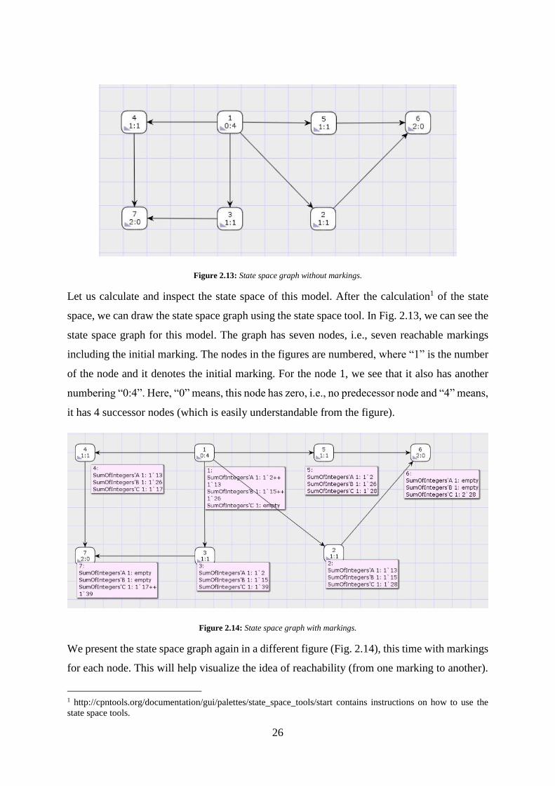
Figure 2.13: State space graph without markings.
Let us calculate and inspect the state space of this model. After the calculation1 of the state
space, we can draw the state space graph using the state space tool. In Fig. 2.13, we can see the
state space graph for this model. The graph has seven nodes, i.e., seven reachable markings
including the initial marking. The nodes in the figures are numbered, where “1” is the number
of the node and it denotes the initial marking. For the node 1, we see that it also has another
numbering “0:4”. Here, “0” means, this node has zero, i.e., no predecessor node and “4” means,
it has 4 successor nodes (which is easily understandable from the figure).
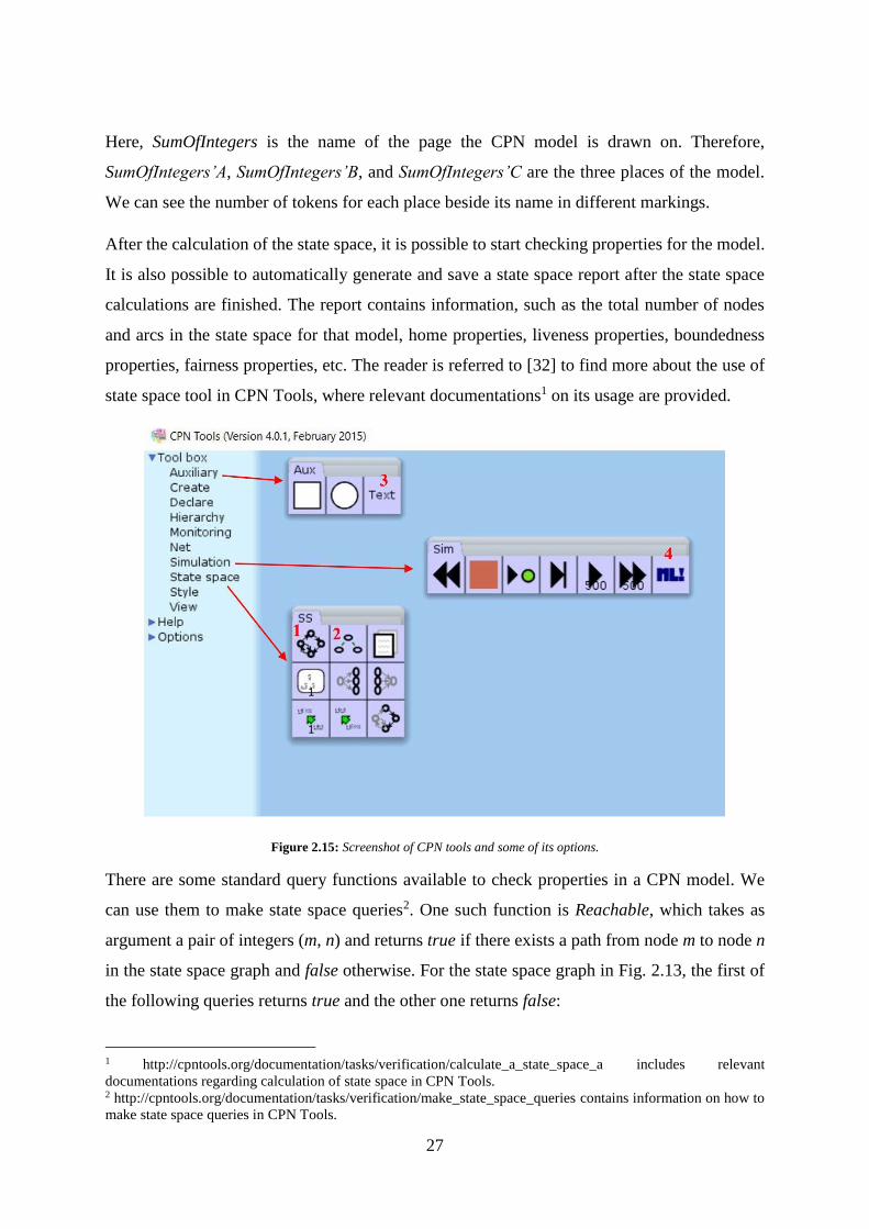
Figure 2.14: State space graph with markings.
We present the state space graph again in a different figure (Fig. 2.14), this time with markings
for each node. This will help visualize the idea of reachability (from one marking to another).
1 http://cpntools.org/documentation/gui/palettes/state_space_tools/start contains instructions on how to use the
state space tools.
27
Here, SumOfIntegers is the name of the page the CPN model is drawn on. Therefore,
SumOfIntegers’A, SumOfIntegers’B, and SumOfIntegers’C are the three places of the model.
We can see the number of tokens for each place beside its name in different markings.
After the calculation of the state space, it is possible to start checking properties for the model.
It is also possible to automatically generate and save a state space report after the state space
calculations are finished. The report contains information, such as the total number of nodes
and arcs in the state space for that model, home properties, liveness properties, boundedness
properties, fairness properties, etc. The reader is referred to [32] to find more about the use of
state space tool in CPN Tools, where relevant documentations1 on its usage are provided.
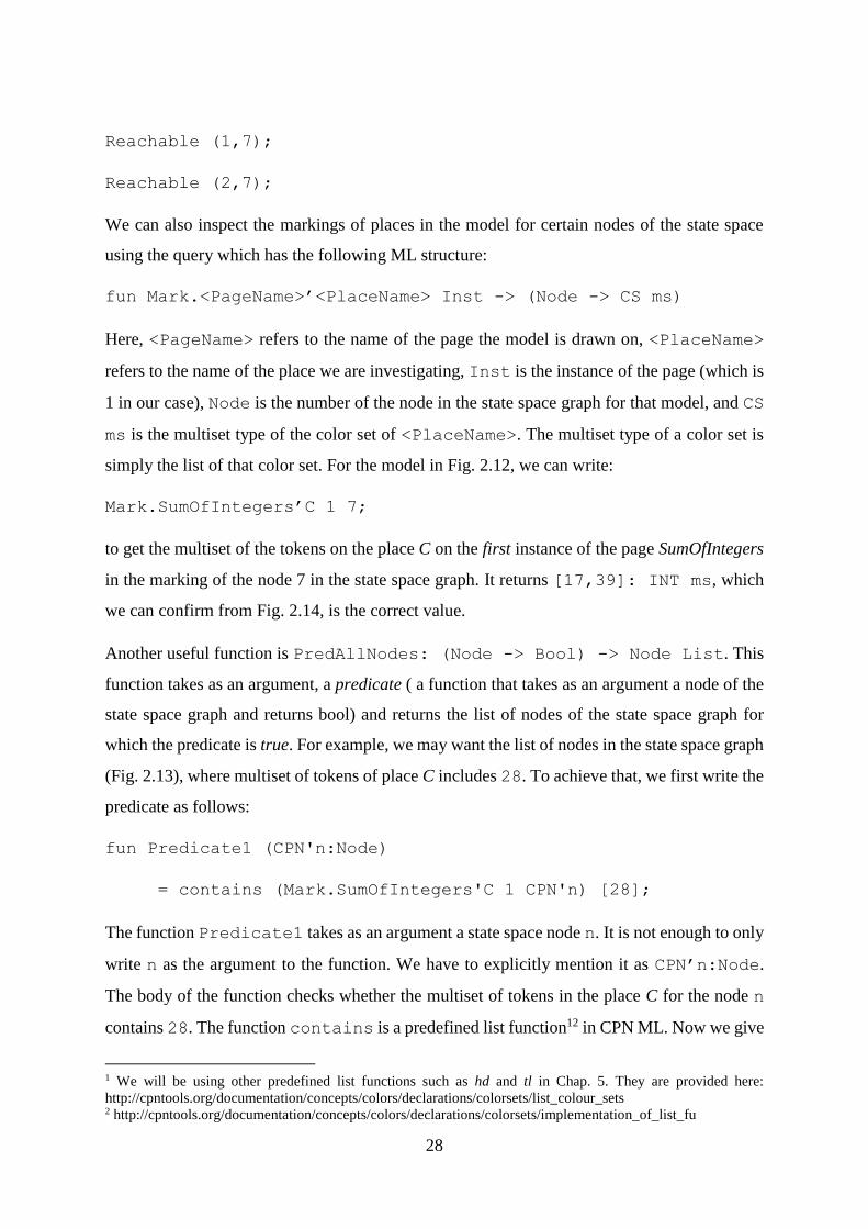
Figure 2.15: Screenshot of CPN tools and some of its options.
There are some standard query functions available to check properties in a CPN model. We
can use them to make state space queries2. One such function is Reachable, which takes as
argument a pair of integers (m, n) and returns true if there exists a path from node m to node n
in the state space graph and false otherwise. For the state space graph in Fig. 2.13, the first of
the following queries returns true and the other one returns false:
1 http://cpntools.org/documentation/tasks/verification/calculate_a_state_space_a includes relevant
documentations regarding calculation of state space in CPN Tools. 2 http://cpntools.org/documentation/tasks/verification/make_state_space_queries contains information on how to
make state space queries in CPN Tools.
28
Reachable (1,7);
Reachable (2,7);
We can also inspect the markings of places in the model for certain nodes of the state space
using the query which has the following ML structure:
fun Mark.<PageName>’<PlaceName> Inst -> (Node -> CS ms)
Here, <PageName> refers to the name of the page the model is drawn on, <PlaceName>
refers to the name of the place we are investigating, Inst is the instance of the page (which is
1 in our case), Node is the number of the node in the state space graph for that model, and CS
ms is the multiset type of the color set of <PlaceName>. The multiset type of a color set is
simply the list of that color set. For the model in Fig. 2.12, we can write:
Mark.SumOfIntegers’C 1 7;
to get the multiset of the tokens on the place C on the first instance of the page SumOfIntegers
in the marking of the node 7 in the state space graph. It returns [17,39]: INT ms, which
we can confirm from Fig. 2.14, is the correct value.
Another useful function is PredAllNodes: (Node -> Bool) -> Node List. This
function takes as an argument, a predicate ( a function that takes as an argument a node of the
state space graph and returns bool) and returns the list of nodes of the state space graph for
which the predicate is true. For example, we may want the list of nodes in the state space graph
(Fig. 2.13), where multiset of tokens of place C includes 28. To achieve that, we first write the
predicate as follows:
fun Predicate1 (CPN'n:Node)
= contains (Mark.SumOfIntegers'C 1 CPN'n) [28];
The function Predicate1 takes as an argument a state space node n. It is not enough to only
write n as the argument to the function. We have to explicitly mention it as CPN’n:Node.
The body of the function checks whether the multiset of tokens in the place C for the node n
contains 28. The function contains is a predefined list function12 in CPN ML. Now we give
1 We will be using other predefined list functions such as hd and tl in Chap. 5. They are provided here:
http://cpntools.org/documentation/concepts/colors/declarations/colorsets/list_colour_sets 2 http://cpntools.org/documentation/concepts/colors/declarations/colorsets/implementation_of_list_fu
29
Predicate1 as an argument to PredAllNodes, which searches the entire state space and
returns a list of nodes for which Predicate1 returns true. In other words, we get a list of
nodes (reachable markings), for which the place C contains a token with the value 28. It is
written as follows:
PredAllNodes Predicate1;
This returns [6,5,2] : Node List, which we can confirm from Fig. 2.14, is correct.
The query can also be written in a different form as follows:
PredAllNodes (fn (CPN'n:Node)
=> contains (Mark.SumOfIntegers'C 1 CPN'n) [28])
In this form, we directly write the body of the function Predicate1 in the query using the
notation (fn arguments => body). This way, we do not have to define separate functions
each time we need to change something in the body of the function.
It is also possible to check properties using non-standard queries, which can be created by
writing CPN ML functions. There is a good amount of predefined state space functions
available in [32] and mostly in [33], which can be used to check properties in CPN models.
Queries are written using the text (marked as “3” in Fig. 2.15) option provided by the Auxiliary
tool palette under the tool box in CPN Tools. After writing the query, it can be evaluated (to
boolean values: true or false) using the Evaluate ML (marked as “4” in Fig. 2.15) option in the
Simulation tool palette under the tool box. However, before making any queries for a CPN
model, the calculation of state space of that model is a prerequisite (using the options marked
as “1” and “2” in Fig. 2.15). A screenshot of the graphical user interface of CPN Tools is
provided along with the aforementioned options and tool palettes in Fig. 2.15.
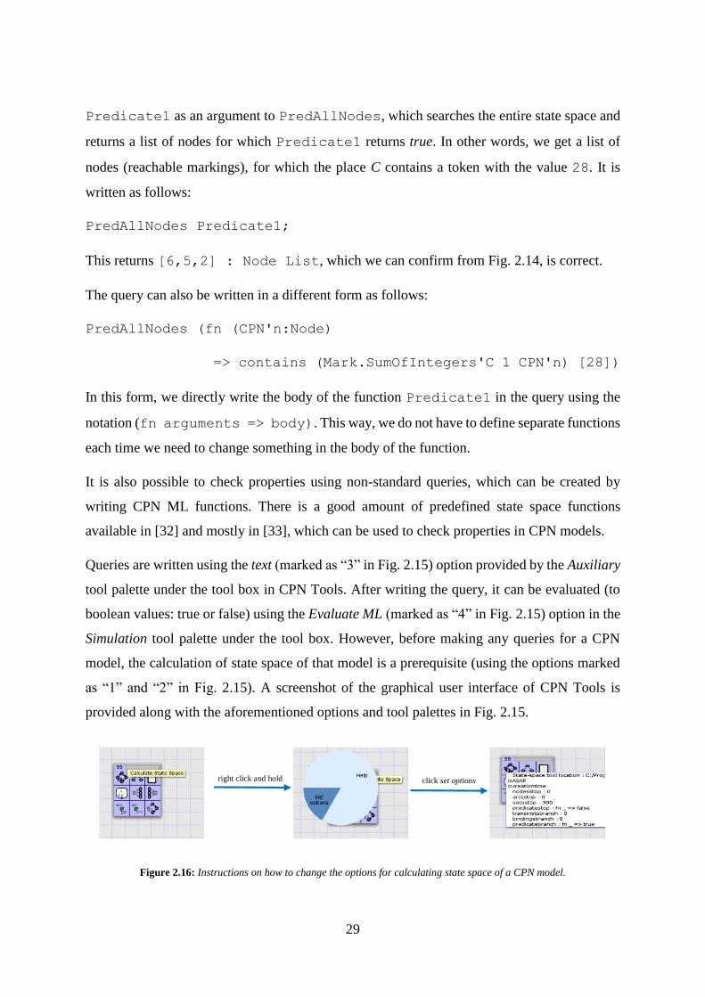
Figure 2.16: Instructions on how to change the options for calculating state space of a CPN model.
right click and hold click set options

30
It is possible to change options for calculating the state space. In Fig. 2.16 we show how to
access those. Sometimes, it is the case that the state space for a model is really big. For such
cases, it is convenient to change some options for calculating the state space. In Fig. 2.16, the
first four options (nodesstop, arcsstop, secsstop, and predicatestop) are called stop options and
the last three options are called branching options. The stop options help decide when a state
space should end. In the figure, we see the default values for these options, where nodesstop :
0 indicates that calculation will not stop until all the nodes are calculated. Similarly, for
arcsstop 0 indicates that calculation will not stop until all arcs are calculated. Any non-zero
positive value given to either nodesstop or arcsstop will result in the stoppage of calculation of
the state space when that number is reached. For secsstop, the value is by default set to 300,
which means the state space calculation will stop after 300 seconds, even if it is partially
calculated (not fully calculated). Therefore, this option is helpful when calculating a really large
state space. If the option is set to zero for secsstop, the calculation will not stop until the state
space is fully calculated [33]. In Chap. 5, when we perform verification on the CPN model
(which has a really large state space), we use this option in order to ensure full calculation of
the state space for the model.
31
3 Transformation from PA-DFD Models to CPN
Models
In this chapter, we describe an algorithm to transform a PA-DFD to a CPN model. The formal
definition of Colored Petri Nets, discussed in section 2.3.2.2, is used for the algorithm. After
the transformation, we will have a CPN represented by the nine-tuple (𝑃, 𝑇, 𝐴, ∑, 𝑉, 𝐶, 𝐺, 𝐸, 𝐼).
The algorithm is presented using pseudo code which uses a syntax similar to that of current
programming languages and thus facilitates its future implementation.
Let us define a set,
Component = {ExternalEntity, Process, DataStore, Limit, Request, Log, LogStore,
Reason, PolicyStore, Clean}
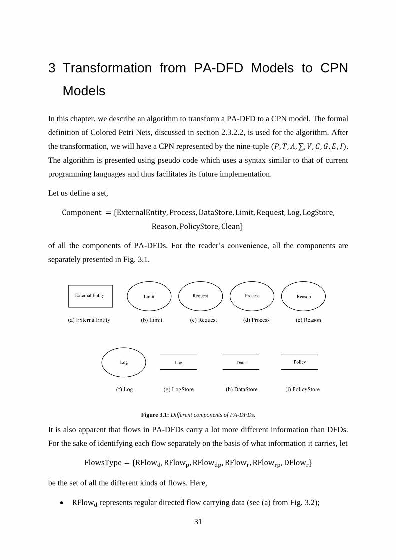
of all the components of PA-DFDs. For the reader’s convenience, all the components are
separately presented in Fig. 3.1.
Figure 3.1: Different components of PA-DFDs.
It is also apparent that flows in PA-DFDs carry a lot more different information than DFDs.
For the sake of identifying each flow separately on the basis of what information it carries, let
FlowsType = {RFlowd, RFlowp, RFlowdp, RFlowr, RFlowrp, DFlowr}
be the set of all the different kinds of flows. Here,
RFlowd represents regular directed flow carrying data (see (a) from Fig. 3.2);
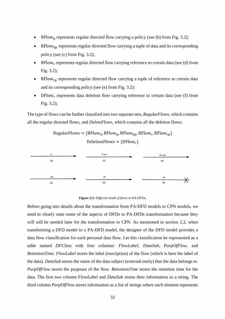
32
RFlowp represents regular directed flow carrying a policy (see (b) from Fig. 3.2);
RFlowdp represents regular directed flow carrying a tuple of data and its corresponding
policy (see (c) from Fig. 3.2);
RFlowr represents regular directed flow carrying reference to certain data (see (d) from
Fig. 3.2);
RFlowrp represents regular directed flow carrying a tuple of reference to certain data
and its corresponding policy (see (e) from Fig. 3.2);
DFlowr represents data deletion flow carrying reference to certain data (see (f) from
Fig. 3.2);
The type of flows can be further classified into two separate sets, RegularFlows, which contains
all the regular directed flows, and DeleteFlows, which contains all the deletion flows:
RegularFlows = {RFlowd, RFlowp, RFlowdp, RFlowr, RFlowrp}
DeletionFlows = {DFlowr}
Figure 3.2: Different kinds of flows in PA-DFDs.
Before going into details about the transformation from PA-DFD models to CPN models, we
need to clearly state some of the aspects of DFDs to PA-DFDs transformation because they
will still be needed later for the transformation to CPN. As mentioned in section 2.2, when
transforming a DFD model to a PA-DFD model, the designer of the DFD model provides a
data flow classification for each personal data flow. Let this classification be represented as a
table named DFClass with four columns: FlowLabel, DataSub, PurpOfFlow, and
RetentionTime. FlowLabel stores the label (inscription) of the flow (which is here the label of
the data). DataSub stores the name of the data subject (external entity) that the data belongs to.
PurpOfFlow stores the purposes of the flow. RetentionTime stores the retention time for the
data. The first two column FlowLabel and DataSub stores their information as a string. The
third column PurpOfFlow stores information as a list of strings where each element represents
33
a single purpose. The stored information in RetentionTime is represented as a non-negative
integer.
Along with the aforementioned four columns, we add a fifth column PolList for the
convenience of PA-DFD to CPN transformation. This column stores the list of labels of all the
flows of type RFlowp that correspond to the personal data in the row. This will help us to
identify which policy flow corresponds to which personal data flow at the time of
transformation. An example row of the table is as follows:
("d", "user", ["research", "advertise"],10, ["p1", "p2"])
From this example, we can say the personal data flow labeled “d” has two corresponding policy
flows (RFlowp) labeled “p1” and “p2”.
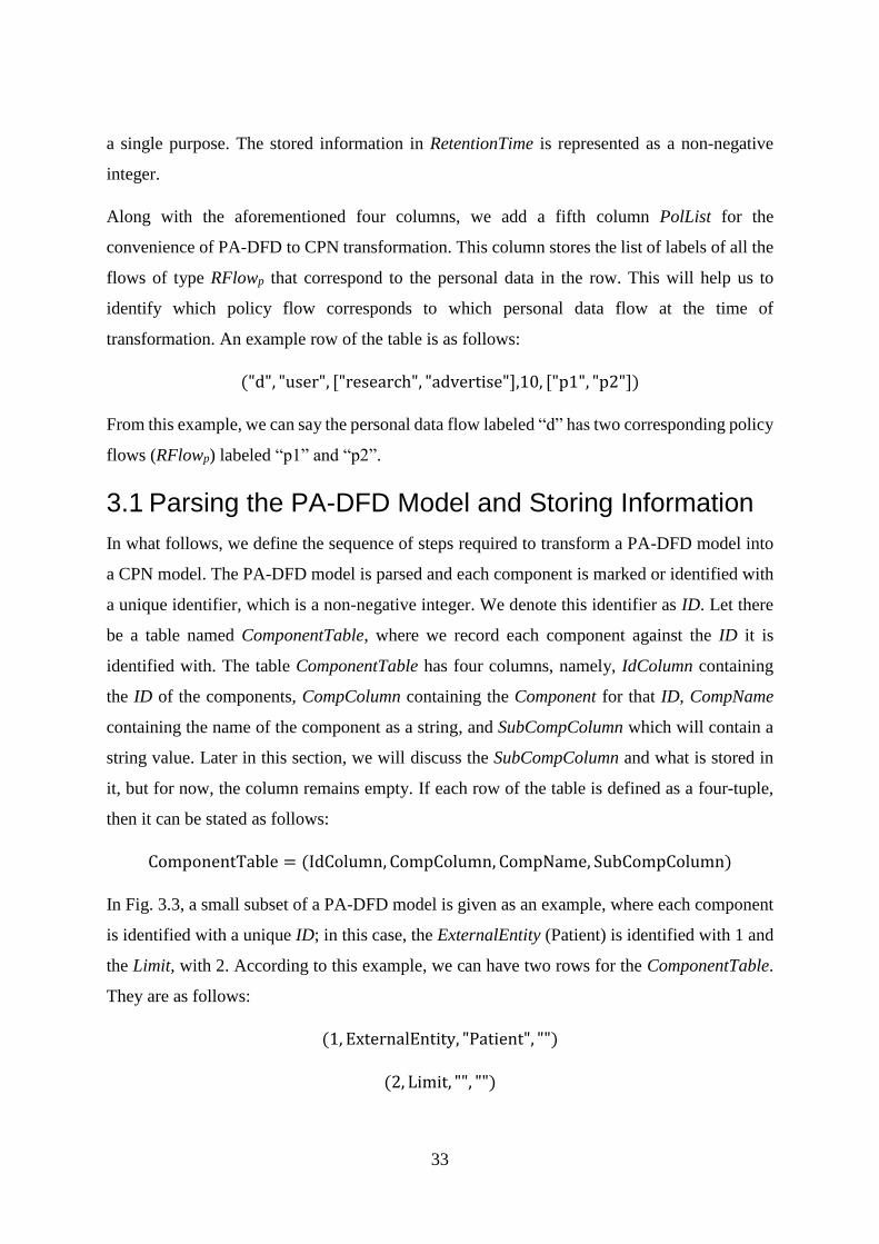
3.1 Parsing the PA-DFD Model and Storing Information
In what follows, we define the sequence of steps required to transform a PA-DFD model into
a CPN model. The PA-DFD model is parsed and each component is marked or identified with
a unique identifier, which is a non-negative integer. We denote this identifier as ID. Let there
be a table named ComponentTable, where we record each component against the ID it is
identified with. The table ComponentTable has four columns, namely, IdColumn containing
the ID of the components, CompColumn containing the Component for that ID, CompName
containing the name of the component as a string, and SubCompColumn which will contain a
string value. Later in this section, we will discuss the SubCompColumn and what is stored in
it, but for now, the column remains empty. If each row of the table is defined as a four-tuple,
then it can be stated as follows:
ComponentTable = (IdColumn, CompColumn, CompName, SubCompColumn)
In Fig. 3.3, a small subset of a PA-DFD model is given as an example, where each component
is identified with a unique ID; in this case, the ExternalEntity (Patient) is identified with 1 and
the Limit, with 2. According to this example, we can have two rows for the ComponentTable.
They are as follows:
(1, ExternalEntity, "Patient", "")
(2, Limit, "", "")
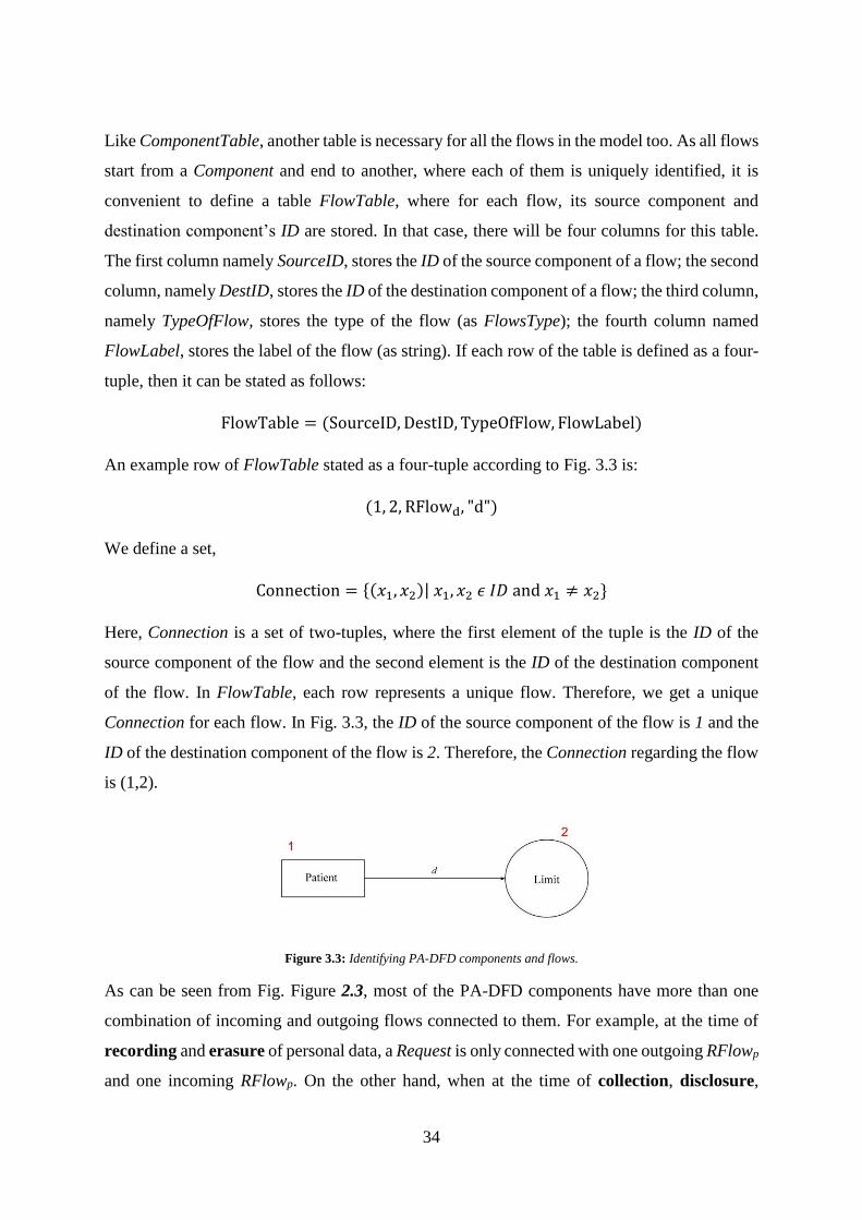
34
Like ComponentTable, another table is necessary for all the flows in the model too. As all flows
start from a Component and end to another, where each of them is uniquely identified, it is
convenient to define a table FlowTable, where for each flow, its source component and
destination component’s ID are stored. In that case, there will be four columns for this table.
The first column namely SourceID, stores the ID of the source component of a flow; the second
column, namely DestID, stores the ID of the destination component of a flow; the third column,
namely TypeOfFlow, stores the type of the flow (as FlowsType); the fourth column named
FlowLabel, stores the label of the flow (as string). If each row of the table is defined as a four-
tuple, then it can be stated as follows:
FlowTable = (SourceID, DestID, TypeOfFlow, FlowLabel)
An example row of FlowTable stated as a four-tuple according to Fig. 3.3 is:
(1, 2, RFlowd, "d")
We define a set,
Connection = {(𝑥1, 𝑥2)| 𝑥1, 𝑥2 𝜖 𝐼𝐷 and 𝑥1 ≠ 𝑥2}
Here, Connection is a set of two-tuples, where the first element of the tuple is the ID of the
source component of the flow and the second element is the ID of the destination component
of the flow. In FlowTable, each row represents a unique flow. Therefore, we get a unique
Connection for each flow. In Fig. 3.3, the ID of the source component of the flow is 1 and the
ID of the destination component of the flow is 2. Therefore, the Connection regarding the flow
is (1,2).
Figure 3.3: Identifying PA-DFD components and flows.
As can be seen from Fig. Figure 2.3, most of the PA-DFD components have more than one
combination of incoming and outgoing flows connected to them. For example, at the time of
recording and erasure of personal data, a Request is only connected with one outgoing RFlowp
and one incoming RFlowp. On the other hand, when at the time of collection, disclosure,
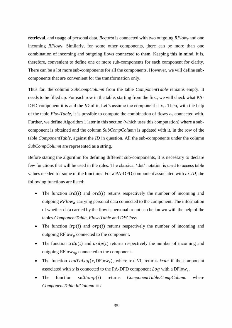
35
retrieval, and usage of personal data, Request is connected with two outgoing RFlowp and one
incoming RFlowp. Similarly, for some other components, there can be more than one
combination of incoming and outgoing flows connected to them. Keeping this in mind, it is,
therefore, convenient to define one or more sub-components for each component for clarity.
There can be a lot more sub-components for all the components. However, we will define sub-
components that are convenient for the transformation only.
Thus far, the column SubCompColumn from the table ComponentTable remains empty. It
needs to be filled up. For each row in the table, starting from the first, we will check what PA-
DFD component it is and the ID of it. Let’s assume the component is 𝑐1. Then, with the help
of the table FlowTable, it is possible to compute the combination of flows 𝑐1 connected with.
Further, we define Algorithm 1 later in this section (which uses this computation) where a sub-
component is obtained and the column SubCompColumn is updated with it, in the row of the
table ComponentTable, against the ID in question. All the sub-components under the column
SubCompColumn are represented as a string.
Before stating the algorithm for defining different sub-components, it is necessary to declare
few functions that will be used in the rules. The classical ‘dot’ notation is used to access table
values needed for some of the functions. For a PA-DFD component associated with 𝑖 𝜖 𝐼𝐷, the
following functions are listed:
The function 𝑖𝑟𝑑(𝑖) and 𝑜𝑟𝑑(𝑖) returns respectively the number of incoming and
outgoing 𝑅𝐹𝑙𝑜𝑤𝑑 carrying personal data connected to the component. The information
of whether data carried by the flow is personal or not can be known with the help of the
tables ComponentTable, FlowsTable and DFClass.
The function 𝑖𝑟𝑝(𝑖) and 𝑜𝑟𝑝(𝑖) returns respectively the number of incoming and
outgoing RFlowp connected to the component.
The function 𝑖𝑟𝑑𝑝(𝑖) and 𝑜𝑟𝑑𝑝(𝑖) returns respectively the number of incoming and
outgoing RFlowdp connected to the component.
The function 𝑐𝑜𝑛𝑇𝑜𝐿𝑜𝑔(𝑥, DFlowr), where 𝑥 𝜖 𝐼𝐷, returns 𝑡𝑟𝑢𝑒 if the component
associated with 𝑥 is connected to the PA-DFD component 𝐿𝑜𝑔 with a DFlowr.
The function 𝑠𝑒𝑙𝐶𝑜𝑚𝑝(𝑖) returns ComponentTable.CompColumn where
ComponentTable.IdColumn ≡ i.
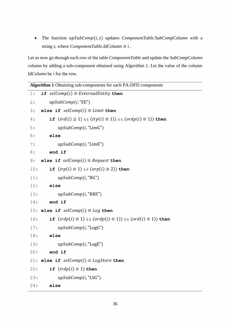
36
The function 𝑢𝑝𝑆𝑢𝑏𝐶𝑜𝑚𝑝(𝑖, 𝑠) updates ComponentTable.SubCompColumn with a
string s, where ComponentTable.IdColumn ≡ i.
Let us now go through each row of the table ComponentTable and update the SubCompColumn
column by adding a sub-component obtained using Algorithm 1. Let the value of the column
IdColumn be i for the row.
Algorithm 1 Obtaining sub-components for each PA-DFD components
1: if 𝑠𝑒𝑙𝐶𝑜𝑚𝑝(𝑖) ≡ 𝐸𝑥𝑡𝑒𝑟𝑛𝑎𝑙𝐸𝑛𝑡𝑖𝑡𝑦 then
2: 𝑢𝑝𝑆𝑢𝑏𝐶𝑜𝑚𝑝(𝑖, "EE")
3: else if 𝑠𝑒𝑙𝐶𝑜𝑚𝑝(𝑖) ≡ 𝐿𝑖𝑚𝑖𝑡 then
4: if (𝑖𝑟𝑑(𝑖) ≥ 1) && (𝑖𝑟𝑝(𝑖) ≡ 1)) && (𝑜𝑟𝑑𝑝(𝑖) ≡ 1)) then
5: 𝑢𝑝𝑆𝑢𝑏𝐶𝑜𝑚𝑝(𝑖, "LimG")
6: else
7: 𝑢𝑝𝑆𝑢𝑏𝐶𝑜𝑚𝑝(𝑖, "LimE")
8: end if
9: else if 𝑠𝑒𝑙𝐶𝑜𝑚𝑝(𝑖) ≡ 𝑅𝑒𝑞𝑢𝑒𝑠𝑡 then
10: if (𝑖𝑟𝑝(𝑖) ≡ 1) && (𝑜𝑟𝑝(𝑖) ≡ 2)) then
11: 𝑢𝑝𝑆𝑢𝑏𝐶𝑜𝑚𝑝(𝑖, "RG")
12: else
13: 𝑢𝑝𝑆𝑢𝑏𝐶𝑜𝑚𝑝(𝑖, "RRE")
14: end if
15: else if 𝑠𝑒𝑙𝐶𝑜𝑚𝑝(𝑖) ≡ 𝐿𝑜𝑔 then
16: if (𝑖𝑟𝑑𝑝(𝑖) ≡ 1) && (𝑜𝑟𝑑𝑝(𝑖) ≡ 1)) && (𝑜𝑟𝑑(𝑖) ≡ 1)) then
17: 𝑢𝑝𝑆𝑢𝑏𝐶𝑜𝑚𝑝(𝑖, "LogG")
18: else
19: 𝑢𝑝𝑆𝑢𝑏𝐶𝑜𝑚𝑝(𝑖, "LogE")
20: end if
21: else if 𝑠𝑒𝑙𝐶𝑜𝑚𝑝(𝑖) ≡ 𝐿𝑜𝑔𝑆𝑡𝑜𝑟𝑒 then
22: if (𝑖𝑟𝑑𝑝(𝑖) ≡ 1) then
23: 𝑢𝑝𝑆𝑢𝑏𝐶𝑜𝑚𝑝(𝑖, "LSG")
24: else
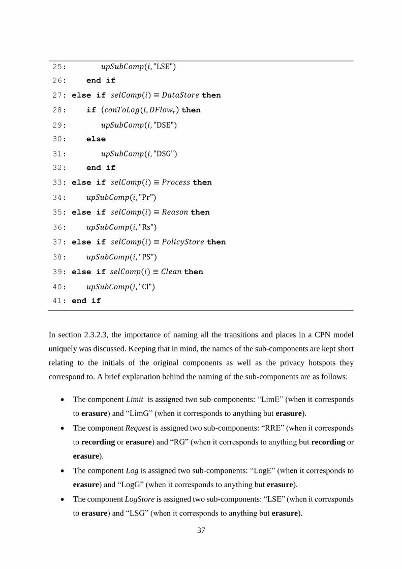
37
25: 𝑢𝑝𝑆𝑢𝑏𝐶𝑜𝑚𝑝(𝑖, "LSE")
26: end if
27: else if 𝑠𝑒𝑙𝐶𝑜𝑚𝑝(𝑖) ≡ 𝐷𝑎𝑡𝑎𝑆𝑡𝑜𝑟𝑒 then
28: if (𝑐𝑜𝑛𝑇𝑜𝐿𝑜𝑔(𝑖, 𝐷𝐹𝑙𝑜𝑤𝑟) then
29: 𝑢𝑝𝑆𝑢𝑏𝐶𝑜𝑚𝑝(𝑖, "DSE")
30: else
31: 𝑢𝑝𝑆𝑢𝑏𝐶𝑜𝑚𝑝(𝑖, "DSG")
32: end if
33: else if 𝑠𝑒𝑙𝐶𝑜𝑚𝑝(𝑖) ≡ 𝑃𝑟𝑜𝑐𝑒𝑠𝑠 then
34: 𝑢𝑝𝑆𝑢𝑏𝐶𝑜𝑚𝑝(𝑖, "Pr")
35: else if 𝑠𝑒𝑙𝐶𝑜𝑚𝑝(𝑖) ≡ 𝑅𝑒𝑎𝑠𝑜𝑛 then
36: 𝑢𝑝𝑆𝑢𝑏𝐶𝑜𝑚𝑝(𝑖, "Rs")
37: else if 𝑠𝑒𝑙𝐶𝑜𝑚𝑝(𝑖) ≡ 𝑃𝑜𝑙𝑖𝑐𝑦𝑆𝑡𝑜𝑟𝑒 then
38: 𝑢𝑝𝑆𝑢𝑏𝐶𝑜𝑚𝑝(𝑖, "PS")
39: else if 𝑠𝑒𝑙𝐶𝑜𝑚𝑝(𝑖) ≡ 𝐶𝑙𝑒𝑎𝑛 then
40: 𝑢𝑝𝑆𝑢𝑏𝐶𝑜𝑚𝑝(𝑖, "Cl")
41: end if
In section 2.3.2.3, the importance of naming all the transitions and places in a CPN model
uniquely was discussed. Keeping that in mind, the names of the sub-components are kept short
relating to the initials of the original components as well as the privacy hotspots they
correspond to. A brief explanation behind the naming of the sub-components are as follows:
The component Limit is assigned two sub-components: “LimE” (when it corresponds
to erasure) and “LimG” (when it corresponds to anything but erasure).
The component Request is assigned two sub-components: “RRE” (when it corresponds
to recording or erasure) and “RG” (when it corresponds to anything but recording or
erasure).
The component Log is assigned two sub-components: “LogE” (when it corresponds to
erasure) and “LogG” (when it corresponds to anything but erasure).
The component LogStore is assigned two sub-components: “LSE” (when it corresponds
to erasure) and “LSG” (when it corresponds to anything but erasure).
38
The component DataStore is assigned two sub-componens: “DSE” (when it
corresponds to erasure) and “DSG” (when it corresponds to anything but erasure).
For each of the components ExternalEntity, Process, Reason, PolicyStore and Clean,
there is no more than a single sub-component. They are respectively named as “EE”,
“Pr”, “Rs”, “PS”, and “Cl”. We assign sub-components to these also in order to be
consistent. As we will be going through the ComponentTable and reading the column
for SubCompColumn for performing the transformation, we want all components to
have a sub-component. We also use the name of the sub-components (because of their
short naming) while naming the places and transition in the CPN model that we obtain
after the transformation.
After applying the Algorithm 1 for each row in ComponentTable, we are ready to start
transforming the given PA-DFD model to a CPN model. However, we need to set up the
environment for the CPN model by defining appropriate color sets, functions and variable
declarations. This is discussed in the next section.
3.2 Definition of Color Sets, Functions and Variable
Declaration
When constructing a CPN model, the prerequisites are to have the necessary color sets,
functions and variables declared. These are the building blocks to express a model effectively.
To get a meaningful CPN model after transforming a PA-DFD model, necessary color sets,
functions and variables need to be defined beforehand too. The color sets for the model are as
follows:
colset REF = INT;
colset EE_NAME = STRING;
colset D_LABEL = STRING;
colset PR_HISTORY = list STRING;
colset DATA = product REF * EE_NAME * D_LABEL * PR_HISTORY;
colset CONS = list STRING;
colset POL = product REF * CONS;
39
colset DATAxPOL = product DATA * POL;
colset REFxPOL = product REF * POL;
colset LOG = product REF * EE_NAME * D_LABEL * PR_HISTORY * CONS;
The very first thing that needs to be decided for the CPN model is how to represent data as well
as the policy as a token. Each token of a CPN model has a color set attached to it. Therefore,
the color set DATA is defined to represent data. It is a four-tuple that includes a unique identifier
REF (reference) for each data, the name of the data subject (external entity) EE_NAME, which
the data belongs to, the label of the data D_LABEL, and PR_HISTORY, which is a list of strings
representing the list of processes the data has been through. On the other hand, the color set
POL is defined to represent a policy. It is a two-tuple consisting of REF, a unique identifier, for
each policy and CONS, a list of user consents, which is represented as a list of strings.
A policy belongs to personal data. When the REF of a policy p and the REF of data d are equal,
we say, p is a policy of d.
Let us also define how to distinguish personal data from non-personal data in the CPN model
obtained after the transformation. We say, when the REF of data is a non-negative integer, it is
considered personal data. Therefore, the policies should also have a REF which is a non-
negative integer. Alternatively, when a REF of data is ~1 (as mentioned in section 2.3.2, ~ is
the unary minus operator in CPN ML), we say it is a non-personal data.
In addition to the color sets DATA and POL, some other color sets are also defined. The color
set DATAxPOL is defined in order to support the places in the CPN model where data and
policy are together. Similarly, REFxPOL is defined for places where the reference of data and
policy are together. On the other hand, the color set LOG is defined to store relevant information
from certain data and its corresponding policy in a place of the CPN model which corresponds
to the 𝐿𝑜𝑔𝑆𝑡𝑜𝑟𝑒 of the PA-DFD model.
As mentioned in section 2.3.2, a Colored Petri Net is represented as a nine-tuple 𝐶𝑃𝑁 =
(𝑃, 𝑇, 𝐴, ∑, 𝐶, 𝐺, 𝐸, 𝐼) (Def. 3). The set of color sets for the model is as follows:
∑ = {REF,EE_NAME,D_LABEL,PR_HISTORY,DATA,CONS,POL,
DATAxPOL,REFxPOL,LOG}
40
Variables in a CPN model are as important as the color sets themselves. They carry the value
of the color sets from one place to another. The following variables are defined for the CPN
model obtained from the transformation:
var id:REF;
var d1, d2:DATA;
var p1, p2:POL;
The set of typed variables in the model is as follows:
𝑉 = {id:REF,d1:DATA,d2:DATA,p1:POL,p2:POL}
In addition to color sets and variables, some functions are defined to carry out necessary tasks
in the model. They are defined as follows:
fun logInfo(d:DATA, p:POL) = (#1d, #2d, #3d, #4d, #2p);
fun dataLab(d:DATA, label:STRING)= (#1d, #2d, label, #4d);
fun processData(d:DATA, PrName:STRING) = (#1d, #2d, #3d,
PrName::(#4d));
Each of the aforementioned functions has different uses on data and policy in the model. The
function logInfo is used when the relevant information regarding a DATA token and its
corresponding POL token are stored in a place which corresponds to LogStore. The place
corresponding LogStore in the CPN model has the color set LOG assigned to it. Therefore the
function logInfo returns a value of color set LOG. On the other hand, the dataLab function
takes a DATA and a STRING value as arguments and replaces the value of the D_LABEL of
the data with the STRING value. Finally, the function processData adds to the existing
PR_HISTORY of a DATA token, the name of the process that it goes through. It is done so to
have the track of the usage of the data in question. Both dataLab and processData are
used when data go through a transition in the CPN model which corresponds to a process in
the PA-DFD model. Both functions return a value of color set DATA. In CPN ML, #nd is used
to extract the nth element of the tuple d.
As mentioned in section 2.3.2, priorities are used to control the enabling and firing of
transitions. The priorities requiring for the transformed CPN model are as follows:
41
val P_EXTRA_HIGH = 10;
val P_HIGH = 100;
val P_NORMAL = 1000;
val P_LOW = 10000;
In addition to the standard priorities available in CPN Tools, we declare a new priority
P_EXTRA_HIGH, which is higher than the already defined ones.
3.3 Transformations for Sub-components
This section explains the details of the transformation for each sub-components, which in turn
ensures the transformation for all the PA-DFD components. We will make use of the various
tables defined earlier that store relevant information of the PA-DFD model. Details regarding
that were already covered in previous sections of this chapter.
The general idea behind the transformation for each component has one thing in common: each
component of the PA-DFD model, when transformed into corresponding parts of a CPN model,
should contain one or more transitions. As we will later see in section 3.4 when a flow of the
PA-DFD model is transformed into the corresponding parts of a CPN model it contains a single
place with an incoming directed arc and an outgoing directed arc. By doing so, it ensures that
sub-components, after being transformed into corresponding parts of a CPN model, will be
connected to each other in ways they are connected in the PA-DFD model.
In order to make the reader visualize the concept of the transformation, a small and general
illustration of such is shown in Fig. 3.4 with an example. On the left-hand side, some PA-DFD
parts are shown and on the right-hand side, their corresponding CPN transformation. Here, we
see two sub-components a and b of a PA-DFD model. We assume the CPN transformation of
a consists of a place ap and a transition at which are connected by a directed arc. On the other
hand, we assume, the CPN transformation of b is slightly different and consists of two
transitions, bt1 and bt2, which are connected to a place bp by two directed arcs. Then, we see
the CPN transformation for the flow labeled d, which consists of a place dp and is connected
to one incoming and one outgoing arc. Finally, at the bottom left of the figure, when sub-
components a and b are connected by the flow labeled d, on the right-hand side it is shown
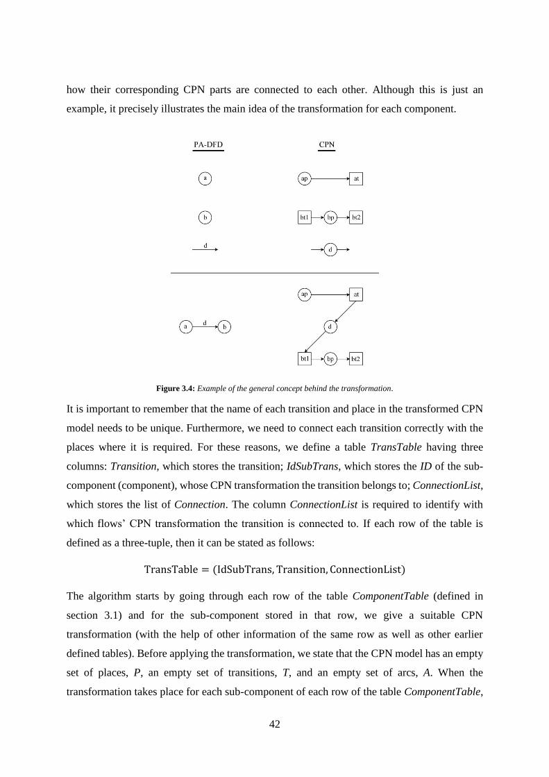
42
how their corresponding CPN parts are connected to each other. Although this is just an
example, it precisely illustrates the main idea of the transformation for each component.
Figure 3.4: Example of the general concept behind the transformation.
It is important to remember that the name of each transition and place in the transformed CPN
model needs to be unique. Furthermore, we need to connect each transition correctly with the
places where it is required. For these reasons, we define a table TransTable having three
columns: Transition, which stores the transition; IdSubTrans, which stores the ID of the sub-
component (component), whose CPN transformation the transition belongs to; ConnectionList,
which stores the list of Connection. The column ConnectionList is required to identify with
which flows’ CPN transformation the transition is connected to. If each row of the table is
defined as a three-tuple, then it can be stated as follows:
TransTable = (IdSubTrans, Transition, ConnectionList)
The algorithm starts by going through each row of the table ComponentTable (defined in
section 3.1) and for the sub-component stored in that row, we give a suitable CPN
transformation (with the help of other information of the same row as well as other earlier
defined tables). Before applying the transformation, we state that the CPN model has an empty
set of places, P, an empty set of transitions, T, and an empty set of arcs, A. When the
transformation takes place for each sub-component of each row of the table ComponentTable,
43
we add suitable elements to these sets. In the transformations, we will also make use of the
color set function 𝐶: 𝑃 → ∑ to assign a color set to a place, the guard function 𝐺: 𝑇 → 𝐸𝑋𝑃𝑅𝑣
to assign a guard to a transition, and the arc expression function 𝐸: 𝐴 → 𝐸𝑋𝑃𝑅𝑣 to assign an
expression to an arc.
In the transformation, a few new functions are used. For a sub-component associated with
𝑖 𝜖 𝐼𝐷, the following functions are listed:
The functions 𝑖𝑟𝑓(𝑖) and 𝑜𝑟𝑓(𝑖) respectively returns the list of Connection for input
and output RegularFlows connected to the sub-component.
The functions 𝑖𝑑𝑓(𝑖) and 𝑜𝑑𝑓(𝑖) respectively returns the list of Connection for input
and output DeletionFlows connected to the sub-component.
The functions 𝑖𝑝𝑓(𝑖) and 𝑜𝑝𝑓(𝑖) respectively returns the list of Connection for input
and output RegularFlows that carry personal data and are connected to the sub-
component.
The functions 𝑖𝑛𝑓𝑙𝑜𝑤(𝑖, 𝑓𝑡) and 𝑜𝑢𝑡𝑓𝑙𝑜𝑤(𝑖, 𝑓𝑡) respectively return the list of
Connection for input flows and list of Connection for output flows that have the type
ft.
The function 𝑝𝑓𝑜𝑟𝑑(𝑑, 𝑙𝑝), given a Connection d of a personal data flow and a list of
Connection lp of flows of type RFlowp (flows that carry policies), returns a single
element from lp whose policy corresponds to the personal data flow of d.
We use the function 𝑙𝑒𝑛𝑔𝑡ℎ(𝑙), which given a list 𝑙, returns the length of the list.
The function 𝑓𝑙((𝑥, 𝑦)), given a Connection as an argument, returns
FlowTable.FlowLabel where FlowTable.SourceID ≡ x and FlowTable.DestID ≡ y.
The function 𝑝𝑙(𝑥), given a label of a flow (which is a string), returns
DFClass.PurpOfFlow where DFClass.FlowName ≡ x.
The function 𝑠𝑒𝑙𝑆𝑢𝑏𝐶𝑜𝑚𝑝(𝑖) returns ComponentTable.SubCompColumn where
ComponentTable.IdColumn ≡ i.
The function 𝑛𝑝(𝑎, 𝑏, 𝑐) is used for generating a place for the CPN model. Here, a is a
string and b & c both are integers. After applying this function on these arguments, the
output is a place, which gets added to the set of places P (if it is already not added
before). The name of the place is the concatenation of all the arguments to the function.
44
For example, 𝑛𝑝("AP", 10,1) should return 𝐴𝑃101 where AP101 𝜖 𝑃. By doing so, it
is ensured that the generated place’s name is unique.
The function 𝑛𝑡(𝑐, 𝑦) is used for generating a transition for the CPN model. Here, x is
a string and y is a list of Connection. After applying this function on these arguments,
the output is a transition, which gets added to the set of transitions T (if it is already not
added before). The name of the transition is the concatenation of all the arguments to
the function. For example, 𝑛𝑡("AT", [(10,1), (20,2)]) should return AT101202 where
AT101202 𝜖 𝑇. By doing so, it is ensured that the generated transition’s name is unique.
If 𝑙 is a non-empty list, the function ℎ𝑑(𝑙) returns the first element of the list. On the
other hand, 𝑡𝑙(𝑙) returns the rest of the list after the first element. For example,
ℎ𝑑([1,2,3]) returns 1, and 𝑡𝑙([1,2,3]) returns [2,3].
The function 𝑟𝑚(𝑙1, 𝑙2) removes all the elements of 𝑙2 which are also members of the
list 𝑙1 and returns the list 𝑙2 with the remaining elements. For example,
𝑟𝑚([1,2], [1,3,4,2,1,4]) returns [3,4,4].
The function 𝑖𝑛𝑠𝑇(𝑥, 𝑦, 𝑧) is used insert a row in the table TransTable, where x
represents the value to be added in column IdSubTrans, y represents the value to be
added in column Transition and z represents the value to be added in column
ConnectionList.
The function 𝑐𝑜𝑛𝑇𝑜(𝑖, 𝑐, 𝑐𝑚𝑝), given i 𝜖 ID, c 𝜖 Connection and cmp 𝜖 Component,
returns the name of cmp. Basically, it returns the name of cmp if it is connected by c to
the component which has the ID i. This can be computed with the help of FlowTable
and ComponentTable.
The function 𝑐𝑜𝑛𝑇𝑜𝑇𝑜(𝑖, 𝑐, 𝑐𝑚𝑝1, 𝑐𝑚𝑝2), given i 𝜖 ID, c 𝜖 Connection and cmp1, cmp2
𝜖 Component, returns the name of cmp2. Basically, it returns the name of cmp2 if it is
connected to cmp1 which is connected by c to another component which has the ID i.
This can be computed with the help of FlowTable and ComponentTable.
The function 𝑐𝑝𝑑(𝑙) given l 𝜖 list of Connection, returns the first occurrence of the
Connection which carries personal data. This can be computed with the help of the
tables FlowTable and DFClass.
The function 𝑒𝑞𝑑𝑙(𝑐, 𝑙𝑐), given c 𝜖 Connection and lc 𝜖 list of Connection, returns a
list of Connection from lc whose flows have the same data label as the data label of the
flow of c.
45
The function 𝑐𝑜𝑛𝑊𝑖𝑡ℎ(𝑙𝑐, 𝑐𝑚𝑝), given lc 𝜖 list of Connection and cmp 𝜖 Component
returns a list of Connection from lc which are connected with cmp.
The function 𝑠𝑒𝑙𝑇𝑟𝑎𝑛𝑠((𝑥, 𝑦), 𝑧), given (𝑥, 𝑦) 𝜖 𝐶𝑜𝑛𝑛𝑒𝑐𝑡𝑖𝑜𝑛 and 𝑧 𝜖 𝐼𝐷, returns
TransTable.Transition where TransTable.IdSubTrans ≡ z and (x,y) is an element of the
list Transtable.ConnectionList.
There is no function available in the formal definition of a Colored Petri Net to assign
a priority to a transition. However, we need to assign certain priorities to different
transitions in the CPN model obtained after the transformation to implement it correctly
in CPN Tools. Therefore, we declare a function 𝑃𝑟𝑖𝑜: 𝑇 → 𝑃𝑟𝑖𝑜𝑟𝑖𝑡𝑦 that assigns a
priority to a transition, where Priority is the set of all the defined priorities. The set with
its elements are as follows:
Priority = {P_EXTRA_HIGH,P_HIGH,P_NORMAL,P_LOW}
We present the algorithms applied for transforming each sub-components of PA-DFDs to
Colored Petri Nets from the sub-section 3.3.1 to the sub-section 3.3.9. Some of the algorithms
may seem too complex. In such cases, we provide example figures. As we will be going through
each row of ComponentTable and apply the appropriate transformation algorithm, let the value
of the column IdColumn be i for that row.
3.3.1 Transformations for Sub-components of ExternalEntity
The PA-DFD component ExternalEntity has a single sub-component, “EE”. For its
transformation, we have to capture several cases where it is connected with only personal data
or only non-personal data or both at the same time. Furthermore, it can be the case where it is
connected with only collection of data or disclosure of data or both at the same time. Keeping
that in mind, the Algorithm 2 is presented capturing all the aforementioned cases.
Algorithm 2 Transformation for sub-component “EE”
1: if 𝑠𝑒𝑙𝑆𝑢𝑏𝐶𝑜𝑚𝑝(𝑖) ≡ "EE" then
2: 𝑙1 = 𝑖𝑝𝑓(𝑖)
3: 𝑙2 = 𝑜𝑝𝑓(𝑖)
4: 𝑙3 = 𝑖𝑛𝑓𝑙𝑜𝑤(𝑖, RFlowp)
5: 𝑙4 = 𝑜𝑢𝑡𝑓𝑙𝑜𝑤(𝑖, RFlowp)
6: 𝑙5 = 𝑖𝑟𝑓(𝑖)

46
7: 𝑙6 = 𝑜𝑟𝑓(𝑖)
8: 𝑙7 = 𝑙1^^𝑙3 /* ”^^” is used to denote concatenation of lists */
9: 𝑙8 = 𝑙2^^𝑙4
10: 𝑙9 = 𝑟𝑚(𝑙7, 𝑙5) /* list of Connection for incoming non-personal data flow */
11: 𝑙10 = 𝑟𝑚(𝑙8, 𝑙6) /* list of Connection for outgoing non-personal data flow */
12: 𝑝1 = 𝑛𝑝("EEP", 𝑖, 1) /* The ‘P’ is added to denote place */
13: 𝐶(𝑝1) = DATAxPOL
14: while (𝑙𝑒𝑛𝑔𝑡ℎ(𝑙1) > 0) do
15: ℎ1 = ℎ𝑑(𝑙1)
16: ℎ𝑝1 = 𝑝𝑓𝑜𝑟𝑑(ℎ1, 𝑙3)
17: ℎℎ𝑝1 = [ℎ1]^^[ℎ𝑝1] /* ”[]” is used to denote list */
18: 𝑡1 = 𝑛𝑡("EET", ℎℎ𝑝1) /* The 'T’ is added to denote transition */
19: 𝑖𝑛𝑠𝑡(𝑖, 𝑡1, ℎℎ𝑝1)
20: {(𝑡1, 𝑝1)} ∪ 𝐴
21: 𝐸((𝑡1, 𝑝1)) =(d1,p1)
22: 𝐺(𝑡2) = ((#1d1)=(#1p1))
23: 𝑙1 = 𝑡𝑙(𝑙1)
24: end while
25: while (𝑙𝑒𝑛𝑔𝑡ℎ(𝑙2) > 0) do
26: ℎ2 = ℎ𝑑(𝑙2)
27: ℎ𝑝2 = 𝑝𝑓𝑜𝑟𝑑(ℎ2, 𝑙4)
28: ℎℎ𝑝2 = [ℎ2]^^[ℎ𝑝2]
29: 𝑡2 = 𝑛𝑡("EET", ℎℎ𝑝2)
30: 𝑖𝑛𝑠𝑡(𝑖, 𝑡2, ℎℎ𝑝2)
31: {(𝑝1, 𝑡2)} ∪ 𝐴
32: 𝐸((𝑝1, 𝑡2)) =(d1,p1)
33: 𝐺(𝑡2) = ((#3d1)=𝑓𝑙(ℎ2))
34: 𝑙2 = 𝑡𝑙(𝑙2)
35: end while
36: while (𝑙𝑒𝑛𝑔𝑡ℎ(𝑙9) > 0) do
47
37: ℎ9 = ℎ𝑑(𝑙9)
38: 𝑡9 = 𝑛𝑡("EET", [ℎ9])
39: 𝑖𝑛𝑠𝑡(𝑖, 𝑡9, [ℎ9])
40: {(𝑡9, 𝑝1)} ∪ 𝐴
41: 𝐸((𝑡9, 𝑝1)) =(d1,(~1,[]))
42: 𝑙9 = 𝑡𝑙(𝑙9)
43: end while
44: while (𝑙𝑒𝑛𝑔𝑡ℎ(𝑙10) > 0) do
45: ℎ10 = ℎ𝑑(𝑙10)
46: 𝑡10 = 𝑛𝑡("EET", [ℎ10])
47: 𝑖𝑛𝑠𝑡(𝑖, 𝑡10, [ℎ10])
48: 𝐺(𝑡10) =(#3d1=𝑓𝑙(ℎ10))
49: {(𝑝1, 𝑡10)} ∪ 𝐴
50: 𝐸((𝑝1, 𝑡10)) =(d1,p1)
51: 𝑙10 = 𝑡𝑙(𝑙10)
52: end while
53: else
54: Apply Algorithm 3
55: end if
The algorithm starts with checking whether the sub-component for that row is “EE”. If it is,
then it proceeds with the rest of the algorithm and transforms it into a CPN representation.
Otherwise, it is some other sub-component and a different algorithm will be applied depending
on which sub-component it is. This is done for all the other algorithms too.
In lines 2-11, necessary lists of Connection for all the different flows that are connected with
the sub-component are stored in different variables separately. An ExternalEntity needs a place
to hold the data and the policies together. In order to facilitate that, a place 𝑝1 is defined in lines
12-13.
In lines 14-24, we work with all the incoming flows carrying personal data to the sub-
component (which corresponds to a disclosure). The variable 𝑙1 stores a list of all the

48
𝐶𝑜𝑛𝑛𝑒𝑐𝑡𝑖𝑜𝑛 of such flows. A Connection ℎ1 from that list is selected in each iteration of the
while loop until the list is empty. We also identify the Connection ℎ𝑝1 of the corresponding
policy flow for the personal data flow that has the Connection ℎ1. A list ℎℎ𝑝1 is created
containing ℎ1 and ℎ𝑝1 as its only elements (line 17). A transition 𝑡1 is created and is recorded
along with the list of Connection ℎℎ𝑝1 and the ID of the sub-component in the table TransTabel
(lines 18-19). This transition will later be identified in order to connect with the CPN
representations of the two flows having the Connection ℎ1 and ℎ2. We create an arc connecting
𝑡1 to 𝑝1 which is added to the set of arcs 𝐴 (line 19) and assign an arc expression to that arc
(line 20). In line 21, we assign a guard to the transition 𝑡1 which specifies in order for a DATA
token and a POL token to go through that transition, they need to have the same reference.
Similarly, In lines 25-35, we work with all the outgoing flows carrying personal data from the
sub-component (which corresponds to a collection). In line 33, the guard on the transition
checks the label of the data d1 in order to make sure that it is indeed the data that is allowed to
go through the transition.
Thus far, in the algorithm, we have been dealing with flows that carry personal data. Flow
carrying non-personal data can also be connected with the sub-component. Let us first take into
consideration the incoming flows carrying non-personal data to the sub-component. The
variable 𝑙9 stores a list of all the 𝐶𝑜𝑛𝑛𝑒𝑐𝑡𝑖𝑜𝑛 of such flows. Then, like before we create a
transition 𝑡9 and an arc connecting that to the place 𝑝1. The arc expression (line 41) is quite
different than the aforementioned two cases regarding personal data flows (lines 21 and 32).
As we are using a place of color set DATAxPOL, we have to make sure the tokens that reside
there also have the same color set. However, non-personal data do not have corresponding
policy that they can make tuple with and form a token of color set DATAxPOL. We have to
take care of that in the arc expression (𝑡9, 𝑝1) by adding an empty policy with the data. This
ensures that everything type-checks.
Similarly, in lines 44-52, we perform the transformation for any outgoing flows carrying non-
personal data from the sub-component. It is quite similar to the transformation for outgoing
flows that carry personal data from the sub-component, except it does not have to deal with
corresponding policy flows because it does not have one.
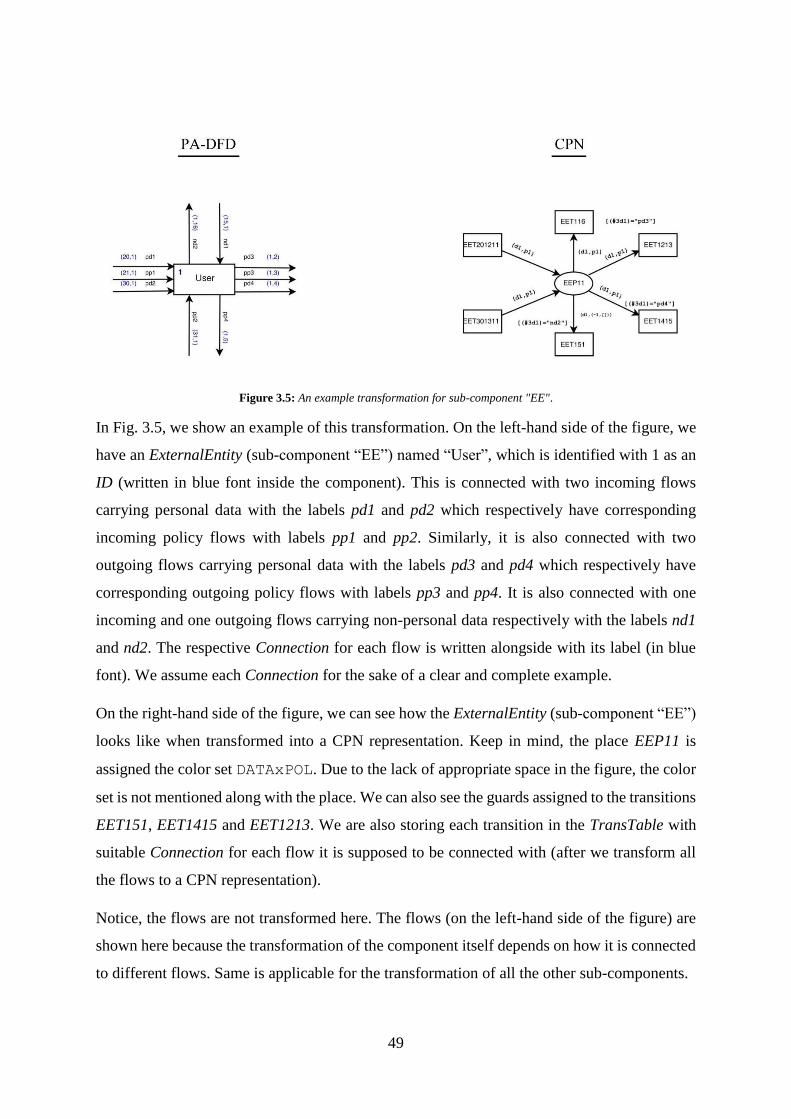
49
Figure 3.5: An example transformation for sub-component "EE".
In Fig. 3.5, we show an example of this transformation. On the left-hand side of the figure, we
have an ExternalEntity (sub-component “EE”) named “User”, which is identified with 1 as an
ID (written in blue font inside the component). This is connected with two incoming flows
carrying personal data with the labels pd1 and pd2 which respectively have corresponding
incoming policy flows with labels pp1 and pp2. Similarly, it is also connected with two
outgoing flows carrying personal data with the labels pd3 and pd4 which respectively have
corresponding outgoing policy flows with labels pp3 and pp4. It is also connected with one
incoming and one outgoing flows carrying non-personal data respectively with the labels nd1
and nd2. The respective Connection for each flow is written alongside with its label (in blue
font). We assume each Connection for the sake of a clear and complete example.
On the right-hand side of the figure, we can see how the ExternalEntity (sub-component “EE”)
looks like when transformed into a CPN representation. Keep in mind, the place EEP11 is
assigned the color set DATAxPOL. Due to the lack of appropriate space in the figure, the color
set is not mentioned along with the place. We can also see the guards assigned to the transitions
EET151, EET1415 and EET1213. We are also storing each transition in the TransTable with
suitable Connection for each flow it is supposed to be connected with (after we transform all
the flows to a CPN representation).
Notice, the flows are not transformed here. The flows (on the left-hand side of the figure) are
shown here because the transformation of the component itself depends on how it is connected
to different flows. Same is applicable for the transformation of all the other sub-components.
50
3.3.2 Transformations for Sub-components of Limit
The PA-DFD component Limit is assigned two sub-components: “LimG” and “LimE”. “LimE”
is present in the model whenever erasure operation takes place. On the other hand, “LimG” is
always present in the model whenever other operations take place.
Algorithm 3 Transformation for sub-component “LimG”
1: if 𝑠𝑒𝑙𝑆𝑢𝑏𝐶𝑜𝑚𝑝(𝑖) ≡ "LimG" then
2: 𝑙1 = 𝑖𝑟𝑓(𝑖)
3: 𝑙2 = 𝑜𝑟𝑓(𝑖)
4: ℎ2 = ℎ𝑑(𝑙2)
5: 𝑙3 = 𝑙1^^𝑙2 /* ”^^” is used to denote concatenation of lists */
6: 𝑝𝑟𝑛 = 𝑐𝑜𝑛𝑇𝑜(𝑖, ℎ2, Process)
7: 𝑒𝑒𝑛 = 𝑐𝑜𝑛𝑇𝑜𝑇𝑜(𝑖, ℎ2, Log, ExternalEntity)
8: 𝑡1 = 𝑛𝑡("LimGT", 𝑙3)
9: 𝑖𝑛𝑠𝑡(𝑖, 𝑡1, 𝑙3)
10: if 𝑝𝑟𝑛 ≠ 𝑛𝑢𝑙𝑙
11: 𝐺(𝑡1) = (((#1d1)=(#1p1))
andalso ((intersect (#2p1) [𝑝𝑟𝑛])<>[]))
12: else if 𝑒𝑒𝑛 ≠ 𝑛𝑢𝑙𝑙
13: 𝐺(𝑡1) = (((#1d1)=(#1p1))
andalso ((intersect (#2p1) [𝑒𝑒𝑛])<>[]))
14: else
15: 𝐺(𝑡1) = (((#1d1)=(#1p1))
andalso ((intersect (#2p1) 𝑝𝑙(𝑓𝑙(𝑐𝑝𝑑(𝑙1))))<>[]))
16: end if
17: else
18: Apply Algorithm 4
19: end if
We present the Algorithm 3 for the transformation of the sub-component “LimG”. Lines 2-5
take care of storing different lists of Connection for different incoming and outgoing flows
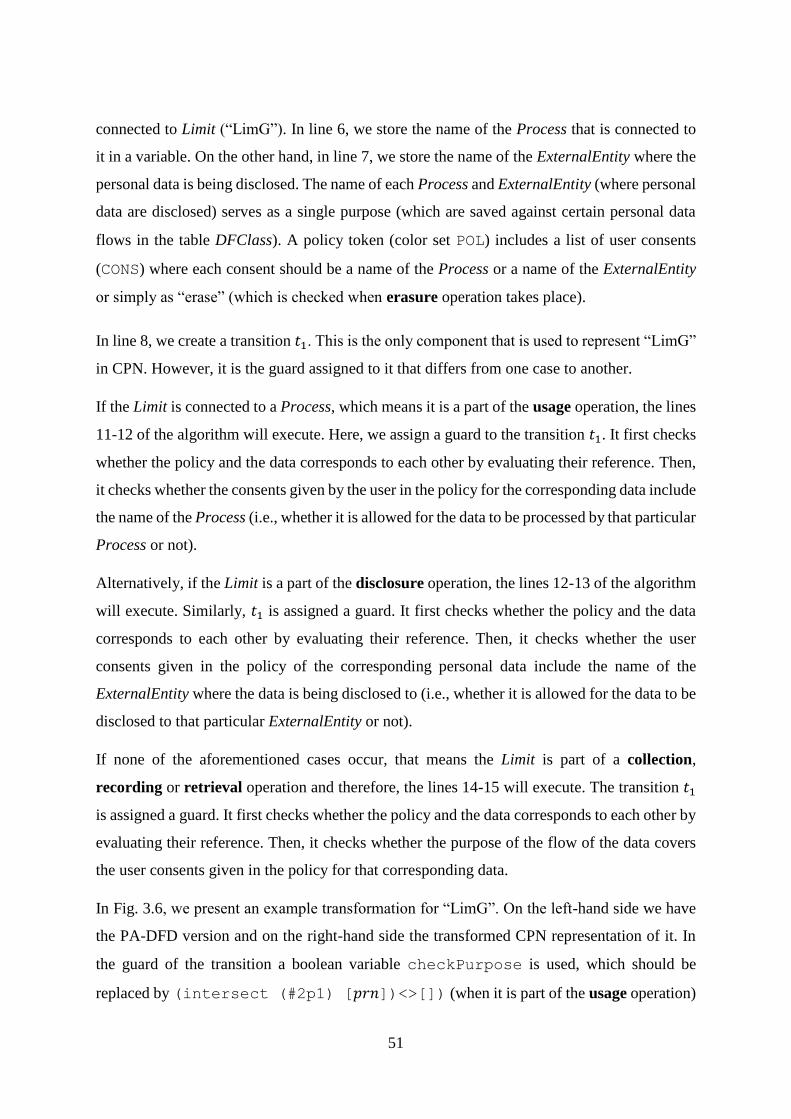
51
connected to Limit (“LimG”). In line 6, we store the name of the Process that is connected to
it in a variable. On the other hand, in line 7, we store the name of the ExternalEntity where the
personal data is being disclosed. The name of each Process and ExternalEntity (where personal
data are disclosed) serves as a single purpose (which are saved against certain personal data
flows in the table DFClass). A policy token (color set POL) includes a list of user consents
(CONS) where each consent should be a name of the Process or a name of the ExternalEntity
or simply as “erase” (which is checked when erasure operation takes place).
In line 8, we create a transition 𝑡1. This is the only component that is used to represent “LimG”
in CPN. However, it is the guard assigned to it that differs from one case to another.
If the Limit is connected to a Process, which means it is a part of the usage operation, the lines
11-12 of the algorithm will execute. Here, we assign a guard to the transition 𝑡1. It first checks
whether the policy and the data corresponds to each other by evaluating their reference. Then,
it checks whether the consents given by the user in the policy for the corresponding data include
the name of the Process (i.e., whether it is allowed for the data to be processed by that particular
Process or not).
Alternatively, if the Limit is a part of the disclosure operation, the lines 12-13 of the algorithm
will execute. Similarly, 𝑡1 is assigned a guard. It first checks whether the policy and the data
corresponds to each other by evaluating their reference. Then, it checks whether the user
consents given in the policy of the corresponding personal data include the name of the
ExternalEntity where the data is being disclosed to (i.e., whether it is allowed for the data to be
disclosed to that particular ExternalEntity or not).
If none of the aforementioned cases occur, that means the Limit is part of a collection,
recording or retrieval operation and therefore, the lines 14-15 will execute. The transition 𝑡1
is assigned a guard. It first checks whether the policy and the data corresponds to each other by
evaluating their reference. Then, it checks whether the purpose of the flow of the data covers
the user consents given in the policy for that corresponding data.
In Fig. 3.6, we present an example transformation for “LimG”. On the left-hand side we have
the PA-DFD version and on the right-hand side the transformed CPN representation of it. In
the guard of the transition a boolean variable checkPurpose is used, which should be
replaced by (intersect (#2p1) [𝑝𝑟𝑛])<>[]) (when it is part of the usage operation)
52
or (intersect (#2p1) [𝑒𝑒𝑛])<>[]) (when it is part of the disclosure operation) or
(intersect (#2p1) 𝑝𝑙(𝑓𝑙(𝑐𝑝𝑑(𝑙1)))<>[]) (when it is part of the collection or
recording or retrieval operation).
Figure 3.6: An example transformation for sub-component "LimG".
Algorithm 4 Transformation for sub-component “LimE”
1: if 𝑠𝑒𝑙𝑆𝑢𝑏𝐶𝑜𝑚𝑝(𝑖) ≡ "LimE" then
2: 𝑙1 = 𝑖𝑟𝑓(𝑖)
3: 𝑙2 = 𝑜𝑟𝑓(𝑖)
4: ℎ2 = ℎ𝑑(𝑙2)
5: 𝑙3 = 𝑙1^^𝑙2 /* ”^^” is used to denote concatenation of lists */
6: 𝑡1 = 𝑛𝑡("LimET", 𝑙3)
7: 𝑖𝑛𝑠𝑡(𝑖, 𝑡1, 𝑙3)
8: 𝐺(𝑡1) = ((id=(#1p1))
andalso ((intersect (#2p1) [“erase”])<>[]))
9: else
10: Apply Algorithm 5
11: end if
53
Algorithm 4 is presented in order to transform the sub-component “LimE”. It is similar in
structure to Algorithm 3, except it is dealing with Limit when it is involved in the erasure
operation. The transformation of “LimE” is represented in CPN by a single transition 𝑡1 and a
guard assigned to it. The guard checks whether the user consents given in the policy for the
corresponding data include the permission for erasing that data. Here, for simplicity check
whether the string “erase” is part of the consents. Due to its close resemblance with the
transformation of “LimG” We do not give an example for “LimE”.
3.3.3 Transformations for Sub-components of Request
The PA-DFD component Limit is assigned two sub-components: “RG” and “RRE”. “RRE” is
present in the model when recording or erasure operation takes place. On the other hand,
“RG” is always present in the model when other operations take place.
Algorithm 5 Transformation for sub-component “RG”
1: if 𝑠𝑒𝑙𝑆𝑢𝑏𝐶𝑜𝑚𝑝(𝑖) ≡ "RG" then
2: 𝑙1 = 𝑖𝑟𝑓(𝑖)
3: 𝑙2 = 𝑜𝑟𝑓(𝑖)
4: 𝑙3 = 𝑙1^^𝑙2 /* ”^^” is used to denote concatenation of lists */
5: 𝑡1 = 𝑛𝑡("RGT", 𝑙3)
6: 𝑖𝑛𝑠𝑡(𝑖, 𝑡1, 𝑙3)
7: 𝑃𝑟𝑖𝑜(𝑡1) = P_HIGH
8: else
9: Apply Algorithm 6
10: end if
Algorithm 5 is presented in order to transform “RG” to CPN representation. It is represented
as a transition 𝑡1 which is created in line 5 of the algorithm. A priority P_HIGH is assigned to
the transition as Request has a priority assigned to it (Fig. Figure 2.3).
Algorithm 6 Transformation for sub-component “RRE”
1: if 𝑠𝑒𝑙𝑆𝑢𝑏𝐶𝑜𝑚𝑝(𝑖) ≡ "RRE" then
2: 𝑙1 = 𝑖𝑟𝑓(𝑖)
3: 𝑙2 = 𝑜𝑟𝑓(𝑖)
54
4: 𝑙3 = 𝑙1^^𝑙2 /* ”^^” is used to denote concatenation of lists */
5: 𝑡1 = 𝑛𝑡("RRET", 𝑙3)
6: 𝑖𝑛𝑠𝑡(𝑖, 𝑡1, 𝑙3)
7: 𝑃𝑟𝑖𝑜(𝑡1) = P_HIGH
8: else
9: Apply Algorithm 7
10: end if
In Algorithm 6, we present the transformation for the sub-component “RRE”. It is almost
identical to Algorithm 5, except the naming of the transition is different.
3.3.4 Transformations for Sub-components of Log
The PA-DFD component Log is assigned two sub-components: “LogG” and “LogE”. “LogE”
is present in the model when erasure operation takes place. On the other hand, “LogG” is
always present in the model when other operations take place.
Algorithm 7 Transformation for sub-component “LogG”
1: if 𝑠𝑒𝑙𝑆𝑢𝑏𝐶𝑜𝑚𝑝(𝑖) ≡ "LogG" then
2: 𝑙1 = 𝑖𝑟𝑓(𝑖)
3: 𝑙2 = 𝑜𝑟𝑓(𝑖)
4: 𝑙3 = 𝑙1^^𝑙2 /* ”^^” is used to denote concatenation of lists */
5: 𝑡1 = 𝑛𝑡("LogGT", 𝑙3)
6: 𝑖𝑛𝑠𝑡(𝑖, 𝑡1, 𝑙3)
7: else
8: Apply Algorithm 8
9: end if
Algorithm 7 is presented in order to transform “LogG” to CPN representation. It is represented
as a transition 𝑡1 which is created in line 5 of the algorithm.
Algorithm 8 Transformation for sub-component “LogE”
1: if 𝑠𝑒𝑙𝑆𝑢𝑏𝐶𝑜𝑚𝑝(𝑖) ≡ "LogE" then
55
2: 𝑙1 = 𝑖𝑟𝑓(𝑖)
3: 𝑙2 = 𝑜𝑟𝑓(𝑖)
4: 𝑙3 = 𝑙1^^𝑙2 /* ”^^” is used to denote concatenation of lists */
5: 𝑡1 = 𝑛𝑡("LogET", 𝑙3)
6: 𝑖𝑛𝑠𝑡(𝑖, 𝑡1, 𝑙3)
7: else
8: Apply Algorithm 9
9: end if
Algorithm 8 is applied when the sub-component is “LogE” and it is similar to Algorithm 7,
except the transition name is different.
3.3.5 Transformations for Sub-components of LogStore
The PA-DFD component LogStore is assigned two sub-components: “LSG” and “LSE”. The
latter is not present in the model unless erasure operation happens and the former is always
present in the model when other operations take place.
Algorithm 9 Transformation for sub-component “LSG”
1: if 𝑠𝑒𝑙𝑆𝑢𝑏𝐶𝑜𝑚𝑝(𝑖) ≡ "LSG" then
2: 𝑡1 = 𝑛𝑡("LSGT", 𝑖𝑟𝑓(𝑖))
3: 𝑖𝑛𝑠𝑡(𝑖, 𝑡1, 𝑖𝑟𝑓(𝑖))
4: 𝑝1 = 𝑛𝑝(”LSGP”, 𝑖, 1)
5: 𝐶(𝑝1) = LOG
6: {(𝑡1, 𝑝1)} ∪ 𝐴
7: 𝐸((𝑡1, 𝑝1)) =logInfo(d1,p1)
8: else
9: Apply Algorithm 10
10: end if
Algorithm 9 is presented in order to transform the sub-component “LSG” to CPN
representation. In line 2 and 4 we create a transition 𝑡1 and a place 𝑝1 respectively. The color
set LOG is assigned to 𝑝1. In line 6, an arc is created and added to the set of all arcs 𝐴. The arc
56
expression for the arc is presented on line 7, where the function logInfo is used in order to
store relevant information in the place 𝑝1.
Algorithm 10 Transformation for sub-component “LSE”
1: if 𝑠𝑒𝑙𝑆𝑢𝑏𝐶𝑜𝑚𝑝(𝑖) ≡ "LSE" then
2: 𝑡1 = 𝑛𝑡("LSET", 𝑖𝑟𝑓(𝑖))
3: 𝑖𝑛𝑠𝑡(𝑖, 𝑡1, 𝑖𝑟𝑓(𝑖))
4: 𝑝1 = 𝑛𝑝(”LSEP”, 𝑖, 1)
5: 𝐶(𝑝1) = REFxPOL
6: {(𝑡1, 𝑝1)} ∪ 𝐴
7: 𝐸((𝑡1, 𝑝1)) = (id,p1)
8: else
9: Apply Algorithm 11
10: end if
Similar to the sub-component “LSG”, we transform “LSE” to CPN transformation using the
Algorithm 10. Algorithms 9 and 10 both are almost similar. However, Algorithm 10 has a place
with a color set of REFxPOL and the arc expression assigned to the arc (at line 7) is different
from Algorithm 9. As “LSE” is connected to an incoming flow of type RFlowrp, it has only
access to the reference of the personal data and the corresponding policy. Therefore, it stores
whatever information it gets from the incoming flow to the place 𝑝1.
3.3.6 Transformations for Sub-components of DataStore
The component DataStore is assigned two sub-components: “DSG” and “DSE”. The former
does not correspond to erasure operation, but the latter does. Due to their names, it gives better
readability for places and transitions while performing verification and is easier to distinguish
between one that deals with erasure operation and one that does not.
Algorithm 11 Transformation for sub-component “DSG”
1: if 𝑠𝑒𝑙𝑆𝑢𝑏𝐶𝑜𝑚𝑝(𝑖) ≡ "DSG" then
2: 𝑙1 = 𝑖𝑟𝑓(𝑖)
3: 𝑙2 = 𝑖𝑑𝑓(𝑖)
57
4: 𝑙3 = 𝑜𝑟𝑓(𝑖)
5: 𝑚1 = 𝑙𝑒𝑛𝑔𝑡ℎ(𝑙1)
6: 𝑚2 = 𝑙𝑒𝑛𝑔𝑡ℎ(𝑙1)
7: 𝑛 = 𝑙𝑒𝑛𝑔𝑡ℎ(𝑙3)
8: 𝑥 = 2
9: 𝑝1 = 𝑛𝑝("DSGP", 𝑖, 1)
10: 𝐶(𝑝1) = DATA
11: 𝑡1 = 𝑛𝑡("DSGT", 𝑙2)
12: 𝑖𝑛𝑠𝑡(𝑖, 𝑡1, 𝑙2)
13: 𝐺(𝑡1) =(id=(#1d1))
14: 𝑃𝑟𝑖𝑜(𝑡1) = P_EXTRA_HIGH
15: {(𝑝1, 𝑡1)} ∪ 𝐴
16: 𝐸((𝑝1, 𝑡1)) = d1
17: while (𝑚1 > 0) do
18: ℎ𝑙1 = ℎ𝑑(𝑙1)
19: 𝑡2 = 𝑛𝑡("DSGT", [ℎ𝑙1]) /* ”[]” is used to denote list */
20: 𝑖𝑛𝑠𝑡(𝑖, 𝑡2, [ℎ𝑙1])
21: {(𝑡2, 𝑝1)} ∪ 𝐴
22: 𝐸((𝑡2, 𝑝1)) = d1
23: 𝑙1 = 𝑡𝑙(𝑙1)
24: 𝑚1 = 𝑚1 − 1
25: end while
26: while (𝑛 > 0) do
27: 𝑙4 = 𝑖𝑟𝑓(𝑖)
28: ℎ𝑙3 = ℎ𝑑(𝑙3)
29: 𝑝2 = 𝑛𝑝(”DSGP”, 𝑖, 𝑥)
30: 𝐶(𝑝2) = DATA
31: 𝑡3 = 𝑛𝑡("DSGT", [ℎ𝑙3])
32: 𝑖𝑛𝑠𝑡(𝑖, 𝑡3, [ℎ𝑙3])
33: 𝐺(𝑡3) =((#1d1)=(#1d2))
58
34: {(𝑡3, 𝑝1), (𝑝1, 𝑡3), (𝑝2, 𝑡3)} ∪ 𝐴
35: 𝐸(𝑎1) = d1 where, 𝑎1 𝜖 {(𝑡3, 𝑝1), (𝑝1, 𝑡3)}
36: 𝐸((𝑝2, 𝑡3)) = d2
37: while (𝑚2 > 0) do
38: ℎ𝑙4 = ℎ𝑑(𝑙4)
39: 𝑡4 = 𝑠𝑒𝑙𝑇𝑟𝑎𝑛𝑠(ℎ𝑙4, 𝑖)
40: {(𝑡4, 𝑝2)} ∪ 𝐴
41: 𝐸((𝑡4, 𝑝2)) = d1
42: 𝑙4 = 𝑡𝑙(𝑙4)
43: 𝑚2 = 𝑚2 − 1
44: end while
45: 𝑙3 = 𝑡𝑙(𝑙3)
46: 𝑛 = 𝑛 − 1
47: 𝑥 = 𝑥 + 1
48: end while
49: else
50: Apply Algorithm 12
51: end if
For the sub-component “DSG”, the Algorithm 11 is applied. Lines 2-7 of the algorithm deals
with storing necessary lists of Connection for each flow (that is connected to the sub-
component) in variables. In line 9 and 10 we create the place 𝑝1 and assign the color set DATA
to it. This place will act as the storage for the DATA token.
The variable 𝑙2 contains the list of Connection for the flow that is connecting the component
Clean to this DataStore (sub-component “DSG”). Lines 11-16 take care of creating the
necessary arc and transition (𝑡1) for the purpose of cleaning data tokens from the place 𝑝1. A
guard is assigned to 𝑡1 in order to check whether the reference sent from the CPN representation
of Clean matches with any of the data token stored in 𝑝1. If so, the data token is sent from 𝑝1
through 𝑡1 for deletion. The priority of 𝑡1 is set to P_EXTRA_HIGH because the cleaning of
the data from a DataStore is of the highest of priorities (as soon as the retention time expires
for certain data, that data is deleted). Although we are not capturing the notion of time in the
59
CPN transformation, we are still presenting a transformation for the component Clean. For that
reason, we need to setup the environment for the CPN transformation of Clean to get connected
with the CPN transformation of “DSG”.
In lines 17-25 we create the necessary amount of transitions and arcs depending on how many
incoming flows are connected with the DataStore.
Figure 3.7: An example transformation for sub-component "DSG".
On the other hand, lines 26-49 deal with setting up the environment (by creating necessary
transitions, places, and arcs) for all the outgoing flows that are connected to the DataStore. For
each outgoing flow, we create a place 𝑝2 with the color set DATA assigned to it and a transition
𝑡3. Then we create three arcs (𝑝2, 𝑡3), (𝑝1, 𝑡3) and (𝑡3, 𝑝1). The place 𝑝1 acts as the storage of
all the data until they are cleaned or erased from it. That is the reason two arcs (𝑝1, 𝑡3) and
(𝑡3, 𝑝1) are created instead of creating only (𝑝1, 𝑡3). This helps the place 𝑝1 store the data
although it forwards it. From lines 37-44, we access all the transitions that was created earlier
in lines 17-25 for all the incoming flows in order to create arcs that connect each of them to the
place 𝑝2.
There is a specific reason for dealing with the outgoing flows connected to the DataStore in
such a way (lines 37-44). It is done to avoid the transition 𝑡3 being always enabled (because of
the arcs (𝑝1, 𝑡3) and (𝑡3, 𝑝1)). If 𝑝1 has a token, then 𝑡3 is always enabled. If that happens, the

60
calculation of state-space does not end as the CPN model then is considered infinite. We avoid
that in lines 37-44 by adding a place 𝑝2. Therefore, when data tokens come, i.e., through the
transitions represented here by 𝑡2, they go to the place 𝑝1 as well as the places represented here
by 𝑝2. Then, when the data are forwarded, they are forwarded from 𝑝1 as well as from all the
places represented here by 𝑝2 through the transitions represented here by 𝑡3 where the guards
on them perform a check. It checks whether the data coming from 𝑝1 and 𝑝2 are equal. If so,
the transitions get enabled and fire the data forward as well as sending them back to the place
𝑝1 as it acts as the storage for data.
In Fig. 3.7, we show an example transformation for “DSG”. We assume the ID of the DataStore
is 5. Also, Connection for each flow is assumed for the sake of the example. One thing to notice
here is the use of double-headed arc between the place DSGP51 and the transition DSGT56.
This arc represents two arcs (one going from the place to the transition and the other going
from the transition to the place) with the same arc expression. CPN Tools supports the use of
such double headed arcs, which increases readability of the model.
The transitions in Fig. 3.7 will be connected by the CPN representation of the PA-DFD flows.
Transitions DSGT35, DSGT45, DSGT25 and DSGT56 will be respectively connected by the
CPN representations of the PA-DFD flows labeled d1, d2, ref1 and d3. We are only presenting
the transformation of the component here, not the flows. That is covered in section 3.4.
The places in Fig. 3.7 have some basic tasks they fulfil. The place DSGP51 acts as the storage
part of DataStore. On the other hand, the place DSGP52 is created in order to only forward the
data token. When data is deleted from DataStore, we need to make sure the data token is deleted
from the place DSGP51. After that, even if DSGP52 contains the data token that was deleted,
it won’t be able to forward the token making it useless.
Algorithm 12 Transformation for sub-component “DSE”
1: if 𝑠𝑒𝑙𝑆𝑢𝑏𝐶𝑜𝑚𝑝(𝑖) ≡ "DSE" then
2: 𝑙1 = 𝑖𝑟𝑓(𝑖)
3: 𝑙2 = 𝐶𝑜𝑛𝑊𝑖𝑡ℎ(𝑖𝑑𝑓(𝑖), Clean)
4: 𝑙3 = 𝑜𝑟𝑓(𝑖)
5: 𝑚1 = 𝑙𝑒𝑛𝑔𝑡ℎ(𝑙1)
6: 𝑚2 = 𝑙𝑒𝑛𝑔𝑡ℎ(𝑙1)
61
7: 𝑛 = 𝑙𝑒𝑛𝑔𝑡ℎ(𝑙3)
8: 𝑥 = 2
9: 𝑝1 = 𝑛𝑝("DSEP", 𝑖, 1)
10: 𝐶(𝑝1) = DATA
11: 𝑡1 = 𝑛𝑡("DSET", 𝑙2)
12: 𝑖𝑛𝑠𝑡(𝑖, 𝑡1, 𝑙2)
13: 𝐺(𝑡1) =(id=(#1d1))
14: 𝑃𝑟𝑖𝑜(𝑡1) = P_EXTRA_HIGH
15: {(𝑝1, 𝑡1)} ∪ 𝐴
16: 𝐸((𝑝1, 𝑡1)) = d1
17: while (𝑚1 > 0) do
18: ℎ𝑙1 = ℎ𝑑(𝑙1)
19: 𝑡2 = 𝑛𝑡("DSET", [ℎ𝑙1]) /* ”[]” is used to denote list */
20: 𝑖𝑛𝑠𝑡(𝑖, 𝑡2, [ℎ𝑙1])
21: {(𝑡2, 𝑝1)} ∪ 𝐴
22: 𝐸((𝑡2, 𝑝1)) = d1
23: 𝑙1 = 𝑡𝑙(𝑙1)
24: 𝑚1 = 𝑚1 − 1
25: end while
26: while (𝑛 > 0) do
27: 𝑙4 = 𝑖𝑟𝑓(𝑖)
28: ℎ𝑙3 = ℎ𝑑(𝑙3)
29: 𝑝2 = 𝑛𝑝(”DSEP”, 𝑖, 𝑥)
30: 𝐶(𝑝2) = DATA
31: 𝑡3 = 𝑛𝑡("DSET", [ℎ𝑙3])
32: 𝑖𝑛𝑠𝑡(𝑖, 𝑡3, [ℎ𝑙3])
33: 𝐺(𝑡3) =((#1d1)=(#1d2))
34: {(𝑡3, 𝑝1), (𝑝1, 𝑡3), (𝑝2, 𝑡3)} ∪ 𝐴
35: 𝐸(𝑎1) = d1 where, 𝑎1 𝜖 {(𝑡3, 𝑝1), (𝑝1, 𝑡3)}
36: 𝐸((𝑝2, 𝑡3)) = d2
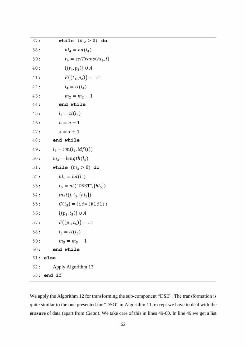
62
37: while (𝑚2 > 0) do
38: ℎ𝑙4 = ℎ𝑑(𝑙4)
39: 𝑡4 = 𝑠𝑒𝑙𝑇𝑟𝑎𝑛𝑠(ℎ𝑙4, 𝑖)
40: {(𝑡4, 𝑝2)} ∪ 𝐴
41: 𝐸((𝑡4, 𝑝2)) = d1
42: 𝑙4 = 𝑡𝑙(𝑙4)
43: 𝑚2 = 𝑚2 − 1
44: end while
45: 𝑙3 = 𝑡𝑙(𝑙3)
46: 𝑛 = 𝑛 − 1
47: 𝑥 = 𝑥 + 1
48: end while
49: 𝑙5 = 𝑟𝑚(𝑙2, 𝑖𝑑𝑓(𝑖))
50: 𝑚3 = 𝑙𝑒𝑛𝑔𝑡ℎ(𝑙5)
51: while (𝑚3 > 0) do
52: ℎ𝑙5 = ℎ𝑑(𝑙5)
53: 𝑡5 = 𝑛𝑡("DSET", [ℎ𝑙5])
54: 𝑖𝑛𝑠𝑡(𝑖, 𝑡5, [ℎ𝑙5])
55: 𝐺(𝑡5) =(id=(#1d1))
56: {(𝑝1, 𝑡5)} ∪ 𝐴
57: 𝐸((𝑝1, 𝑡5)) = d1
58: 𝑙5 = 𝑡𝑙(𝑙5)
59: 𝑚3 = 𝑚3 − 1
60: end while
61: else
62: Apply Algorithm 13
63: end if
We apply the Algorithm 12 for transforming the sub-component “DSE”. The transformation is
quite similar to the one presented for “DSG” in Algorithm 11, except we have to deal with the
erasure of data (apart from Clean). We take care of this in lines 49-60. In line 49 we get a list
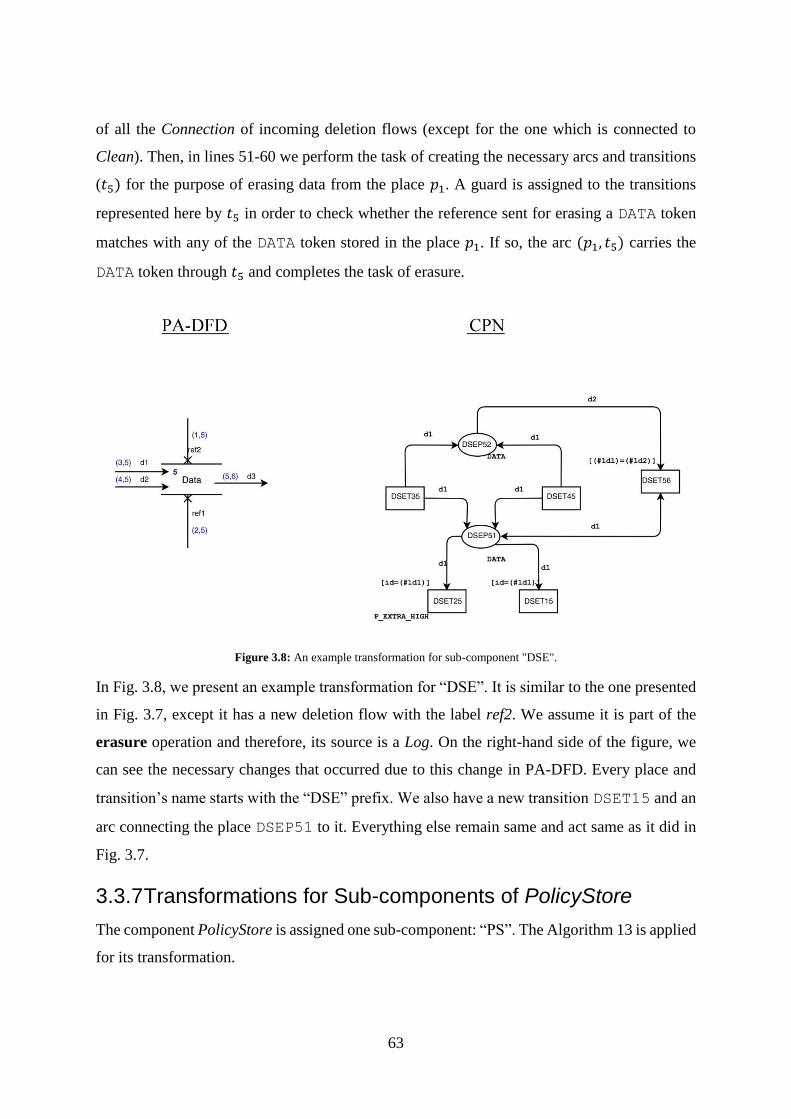
63
of all the Connection of incoming deletion flows (except for the one which is connected to
Clean). Then, in lines 51-60 we perform the task of creating the necessary arcs and transitions
(𝑡5) for the purpose of erasing data from the place 𝑝1. A guard is assigned to the transitions
represented here by 𝑡5 in order to check whether the reference sent for erasing a DATA token
matches with any of the DATA token stored in the place 𝑝1. If so, the arc (𝑝1, 𝑡5) carries the
DATA token through 𝑡5 and completes the task of erasure.
Figure 3.8: An example transformation for sub-component "DSE".
In Fig. 3.8, we present an example transformation for “DSE”. It is similar to the one presented
in Fig. 3.7, except it has a new deletion flow with the label ref2. We assume it is part of the
erasure operation and therefore, its source is a Log. On the right-hand side of the figure, we
can see the necessary changes that occurred due to this change in PA-DFD. Every place and
transition’s name starts with the “DSE” prefix. We also have a new transition DSET15 and an
arc connecting the place DSEP51 to it. Everything else remain same and act same as it did in
Fig. 3.7.
3.3.7 Transformations for Sub-components of PolicyStore
The component PolicyStore is assigned one sub-component: “PS”. The Algorithm 13 is applied
for its transformation.
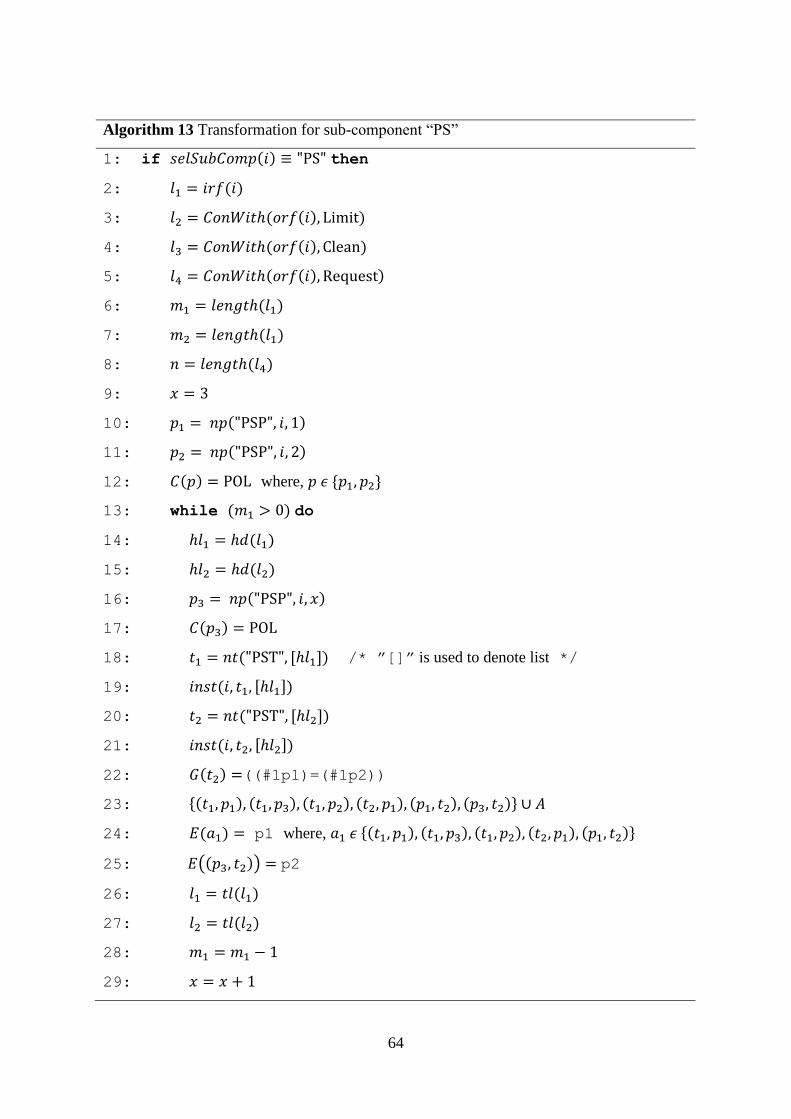
64
Algorithm 13 Transformation for sub-component “PS”
1: if 𝑠𝑒𝑙𝑆𝑢𝑏𝐶𝑜𝑚𝑝(𝑖) ≡ "PS" then
2: 𝑙1 = 𝑖𝑟𝑓(𝑖)
3: 𝑙2 = 𝐶𝑜𝑛𝑊𝑖𝑡ℎ(𝑜𝑟𝑓(𝑖), Limit)
4: 𝑙3 = 𝐶𝑜𝑛𝑊𝑖𝑡ℎ(𝑜𝑟𝑓(𝑖), Clean)
5: 𝑙4 = 𝐶𝑜𝑛𝑊𝑖𝑡ℎ(𝑜𝑟𝑓(𝑖), Request)
6: 𝑚1 = 𝑙𝑒𝑛𝑔𝑡ℎ(𝑙1)
7: 𝑚2 = 𝑙𝑒𝑛𝑔𝑡ℎ(𝑙1)
8: 𝑛 = 𝑙𝑒𝑛𝑔𝑡ℎ(𝑙4)
9: 𝑥 = 3
10: 𝑝1 = 𝑛𝑝("PSP", 𝑖, 1)
11: 𝑝2 = 𝑛𝑝("PSP", 𝑖, 2)
12: 𝐶(𝑝) = POL where, 𝑝 𝜖 {𝑝1, 𝑝2}
13: while (𝑚1 > 0) do
14: ℎ𝑙1 = ℎ𝑑(𝑙1)
15: ℎ𝑙2 = ℎ𝑑(𝑙2)
16: 𝑝3 = 𝑛𝑝("PSP", 𝑖, 𝑥)
17: 𝐶(𝑝3) = POL
18: 𝑡1 = 𝑛𝑡("PST", [ℎ𝑙1]) /* ”[]” is used to denote list */
19: 𝑖𝑛𝑠𝑡(𝑖, 𝑡1, [ℎ𝑙1])
20: 𝑡2 = 𝑛𝑡("PST", [ℎ𝑙2])
21: 𝑖𝑛𝑠𝑡(𝑖, 𝑡2, [ℎ𝑙2])
22: 𝐺(𝑡2) =((#1p1)=(#1p2))
23: {(𝑡1, 𝑝1), (𝑡1, 𝑝3), (𝑡1, 𝑝2), (𝑡2, 𝑝1), (𝑝1, 𝑡2), (𝑝3, 𝑡2)} ∪ 𝐴
24: 𝐸(𝑎1) = p1 where, 𝑎1 𝜖 {(𝑡1, 𝑝1), (𝑡1, 𝑝3), (𝑡1, 𝑝2), (𝑡2, 𝑝1), (𝑝1, 𝑡2)}
25: 𝐸((𝑝3, 𝑡2)) = p2
26: 𝑙1 = 𝑡𝑙(𝑙1)
27: 𝑙2 = 𝑡𝑙(𝑙2)
28: 𝑚1 = 𝑚1 − 1
29: 𝑥 = 𝑥 + 1
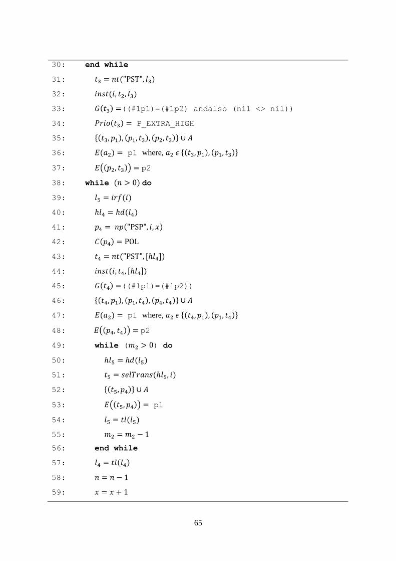
65
30: end while
31: 𝑡3 = 𝑛𝑡("PST", 𝑙3)
32: 𝑖𝑛𝑠𝑡(𝑖, 𝑡2, 𝑙3)
33: 𝐺(𝑡3) =((#1p1)=(#1p2) andalso (nil <> nil))
34: 𝑃𝑟𝑖𝑜(𝑡3) = P_EXTRA_HIGH
35: {(𝑡3, 𝑝1), (𝑝1, 𝑡3), (𝑝2, 𝑡3)} ∪ 𝐴
36: 𝐸(𝑎2) = p1 where, 𝑎2 𝜖 {(𝑡3, 𝑝1), (𝑝1, 𝑡3)}
37: 𝐸((𝑝2, 𝑡3)) = p2
38: while (𝑛 > 0) do
39: 𝑙5 = 𝑖𝑟𝑓(𝑖)
40: ℎ𝑙4 = ℎ𝑑(𝑙4)
41: 𝑝4 = 𝑛𝑝("PSP", 𝑖, 𝑥)
42: 𝐶(𝑝4) = POL
43: 𝑡4 = 𝑛𝑡("PST", [ℎ𝑙4])
44: 𝑖𝑛𝑠𝑡(𝑖, 𝑡4, [ℎ𝑙4])
45: 𝐺(𝑡4) =((#1p1)=(#1p2))
46: {(𝑡4, 𝑝1), (𝑝1, 𝑡4), (𝑝4, 𝑡4)} ∪ 𝐴
47: 𝐸(𝑎2) = p1 where, 𝑎2 𝜖 {(𝑡4, 𝑝1), (𝑝1, 𝑡4)}
48: 𝐸((𝑝4, 𝑡4)) = p2
49: while (𝑚2 > 0) do
50: ℎ𝑙5 = ℎ𝑑(𝑙5)
51: 𝑡5 = 𝑠𝑒𝑙𝑇𝑟𝑎𝑛𝑠(ℎ𝑙5, 𝑖)
52: {(𝑡5, 𝑝4)} ∪ 𝐴
53: 𝐸((𝑡5, 𝑝4)) = p1
54: 𝑙5 = 𝑡𝑙(𝑙5)
55: 𝑚2 = 𝑚2 − 1
56: end while
57: 𝑙4 = 𝑡𝑙(𝑙4)
58: 𝑛 = 𝑛 − 1
59: 𝑥 = 𝑥 + 1
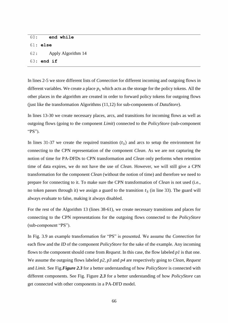
66
60: end while
61: else
62: Apply Algorithm 14
63: end if
In lines 2-5 we store different lists of Connection for different incoming and outgoing flows in
different variables. We create a place 𝑝1 which acts as the storage for the policy tokens. All the
other places in the algorithm are created in order to forward policy tokens for outgoing flows
(just like the transformation Algorithms (11,12) for sub-components of DataStore).
In lines 13-30 we create necessary places, arcs, and transitions for incoming flows as well as
outgoing flows (going to the component Limit) connected to the PolicyStore (sub-component
“PS”).
In lines 31-37 we create the required transition (𝑡3) and arcs to setup the environment for
connecting to the CPN representation of the component Clean. As we are not capturing the
notion of time for PA-DFDs to CPN transformation and Clean only performs when retention
time of data expires, we do not have the use of Clean. However, we will still give a CPN
transformation for the component Clean (without the notion of time) and therefore we need to
prepare for connecting to it. To make sure the CPN transformation of Clean is not used (i.e.,
no token passes through it) we assign a guard to the transition 𝑡3 (in line 33). The guard will
always evaluate to false, making it always disabled.
For the rest of the Algorithm 13 (lines 38-61), we create necessary transitions and places for
connecting to the CPN representations for the outgoing flows connected to the PolicyStore
(sub-component “PS”).
In Fig. 3.9 an example transformation for “PS” is presented. We assume the Connection for
each flow and the ID of the component PolicyStore for the sake of the example. Any incoming
flows to the component should come from Request. In this case, the flow labeled p1 is that one.
We assume the outgoing flows labeled p2, p3 and p4 are respectively going to Clean, Request
and Limit. See Fig.Figure 2.3 for a better understanding of how PolicyStore is connected with
different components. See Fig. Figure 2.3 for a better understanding of how PolicyStore can
get connected with other components in a PA-DFD model.
67
Figure 3.9: An example transformation for sub-component "PS".
The transitions in Fig. 3.9 will be connected by the CPN representation of the PA-DFD flows.
Transitions PSTT35, PST57, PST56 and PST58 will be respectively connected by the CPN
representations of the PA-DFD flows labeled p1, p2, p3 and p4. We are only presenting the
transformation of the component here, not the flows. That is covered in section 3.4.
The places in Fig 3.9 have some basic tasks they fulfil. The place PSP51 acts as the storage
part of PolicyStore. On the other hand, the other places are created in order to only forward the
policy token. When a policy is deleted from PolicyStore, we need to make sure the policy token
is deleted from the place PSP51. After that, even if the other places contain the policy token
that was deleted, they won’t be able to forward the token making it useless.
3.3.8 Transformations for Sub-components of Process and
Reason
The PA-DFD component Process is assigned one sub-component: “Pr”. It can get connected
to different types of incoming and outgoing flows. While dealing with personal data, it can get
connected to one or more incoming and outgoing flows of type RFlowdp. On the other hand,
when it deals with non-personal data, it can get connected to one or more incoming and
outgoing flows of type RFlowd. Apart from these, when the erasure operation takes place, it
68
can get connected with outgoing flows of type RFlowr (that carries the reference of the personal
data to be erased) and RFlowp (that carries the corresponding policy of that personal data). We
assume that, in order to carry out the erasure operation, the Process needs to be provided with
the reference of the personal data as well as the corresponding policy by an incoming flow of
type RFlowrp. It was not strictly mentioned in [4] what type of incoming flow is connected to
the Process for the erasure operation when the author of the thesis was working on this.
Algorithm 14 is applied for transforming the sub-component “Pr”.
Algorithm 14 Transformation for sub-component “Pr”
1: if 𝑠𝑒𝑙𝑆𝑢𝑏𝐶𝑜𝑚𝑝(𝑖) ≡ "Pr" then
2: 𝑙1 = 𝑖𝑛𝑓𝑙𝑜𝑤(𝑖, RFlowdp)
3: 𝑙2 = 𝑜𝑢𝑡𝑓𝑙𝑜𝑤(𝑖, RFlowdp)
4: 𝑙3 = 𝑜𝑢𝑡𝑓𝑙𝑜𝑤(𝑖, RFlowp)
5: 𝑙4 = 𝑜𝑢𝑡𝑓𝑙𝑜𝑤(𝑖, RFlow𝑟)
6: 𝑙5 = 𝑙3^^𝑙4
7: 𝑙6 = 𝑖𝑛𝑓𝑙𝑜𝑤(𝑖, RFlowrp)
8: 𝑙7 = 𝑖𝑛𝑓𝑙𝑜𝑤(𝑖, RFlowd)
9: 𝑙8 = 𝑜𝑢𝑡𝑓𝑙𝑜𝑤(𝑖, RFlowd)
10: if 𝑙𝑒𝑛𝑔𝑡ℎ(𝑙1) > 0 then
11: 𝑡1 = 𝑛𝑡("PrT", 𝑙1)
12: 𝑖𝑛𝑠𝑡(𝑖, 𝑡1, 𝑙1)
13: end if
14: if 𝑙𝑒𝑛𝑔𝑡ℎ(𝑙2) > 0 then
15: 𝑝1 = 𝑛𝑝("PrP", 𝑖, 1)
16: 𝐶(𝑝1) = DATAxPOL
17: if 𝑙𝑒𝑛𝑔𝑡ℎ(𝑙1) > 0 then
18: {(𝑡1, 𝑝1)} ∪ 𝐴
19: 𝐸((𝑡1, 𝑝1)) =(d1,p1)
20: end if
21: 𝑡2 = 𝑛𝑡("PrT", 𝑙2)
22: 𝑖𝑛𝑠𝑡(𝑖, 𝑡2, 𝑙2)
69
23: {(𝑝1, 𝑡2)} ∪ 𝐴
24: 𝐸((𝑝1, 𝑡2)) =(d1,p1)
25: end if
26: if 𝑙𝑒𝑛𝑔𝑡ℎ(𝑙6) > 0 then
27: 𝑡3 = 𝑛𝑡("PrT", 𝑙6)
28: 𝑖𝑛𝑠𝑡(𝑖, 𝑡3, 𝑙6)
29: end if
30: if 𝑙𝑒𝑛𝑔𝑡ℎ(𝑙5) > 0 then
31: 𝑝2 = 𝑛𝑝("PrP", 𝑖, 2)
32: 𝐶(𝑝2) = REFxPOL
33: if 𝑙𝑒𝑛𝑔𝑡ℎ(𝑙1) > 0 then
34: {(𝑡3, 𝑝2)} ∪ 𝐴
35: 𝐸((𝑡3, 𝑝2)) =(id,p1)
36: end if
37: 𝑡4 = 𝑛𝑡("PrT", 𝑙5)
38: 𝑖𝑛𝑠𝑡(𝑖, 𝑡4, 𝑙5)
39: {(𝑝2, 𝑡4)} ∪ 𝐴
40: 𝐸((𝑝2, 𝑡4)) =(id,p1)
41: end if
42: if 𝑙𝑒𝑛𝑔𝑡ℎ(𝑙7) > 0 then
43: while (𝑙𝑒𝑛𝑔𝑡ℎ(𝑙7) > 0) do
44: ℎ𝑙7 = ℎ𝑑(𝑙7)
45: 𝑡5 = 𝑛𝑡("PrT", [ℎ𝑙7])
46: 𝑖𝑛𝑠𝑡(𝑖, 𝑡5, [ℎ𝑙7])
47: 𝑙7 = 𝑡𝑙(𝑙7)
48: end while
49: end if
50: if 𝑙𝑒𝑛𝑔𝑡ℎ(𝑙8) > 0 then
51: 𝑝3 = 𝑛𝑝("PrP", 𝑖, 3)
52: 𝐶(𝑝3) = DATA
53: 𝑙9 = 𝑖𝑛𝑓𝑙𝑜𝑤(𝑖, RFlowd)
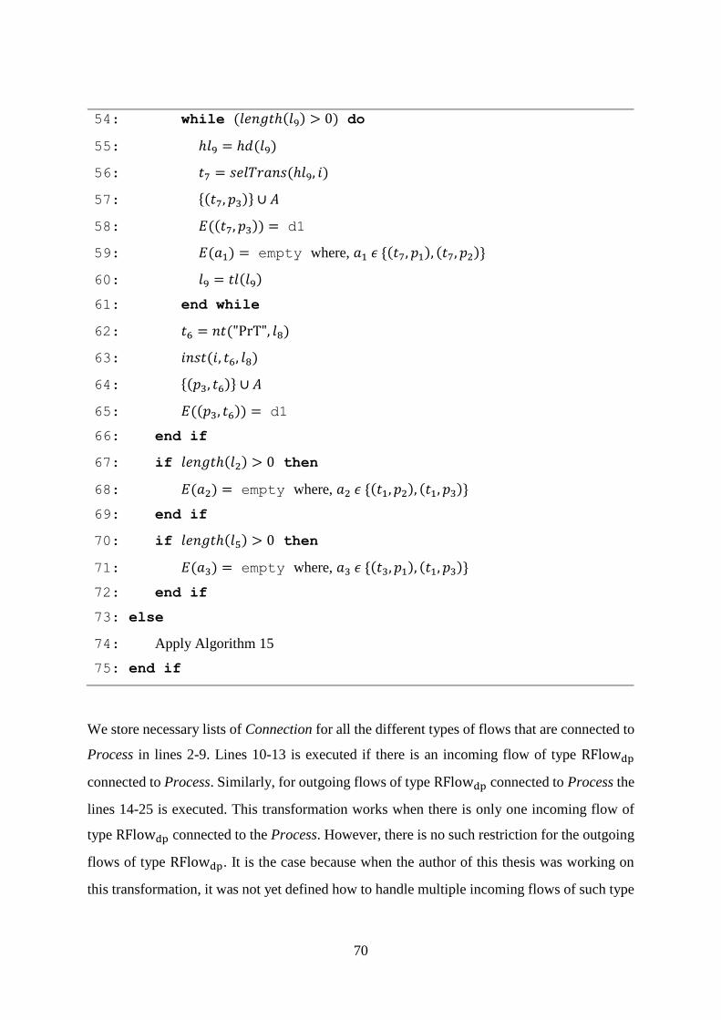
70
54: while (𝑙𝑒𝑛𝑔𝑡ℎ(𝑙9) > 0) do
55: ℎ𝑙9 = ℎ𝑑(𝑙9)
56: 𝑡7 = 𝑠𝑒𝑙𝑇𝑟𝑎𝑛𝑠(ℎ𝑙9, 𝑖)
57: {(𝑡7, 𝑝3)} ∪ 𝐴
58: 𝐸((𝑡7, 𝑝3)) = d1
59: 𝐸(𝑎1) = empty where, 𝑎1 𝜖 {(𝑡7, 𝑝1), (𝑡7, 𝑝2)}
60: 𝑙9 = 𝑡𝑙(𝑙9)
61: end while
62: 𝑡6 = 𝑛𝑡("PrT", 𝑙8)
63: 𝑖𝑛𝑠𝑡(𝑖, 𝑡6, 𝑙8)
64: {(𝑝3, 𝑡6)} ∪ 𝐴
65: 𝐸((𝑝3, 𝑡6)) = d1
66: end if
67: if 𝑙𝑒𝑛𝑔𝑡ℎ(𝑙2) > 0 then
68: 𝐸(𝑎2) = empty where, 𝑎2 𝜖 {(𝑡1, 𝑝2), (𝑡1, 𝑝3)}
69: end if
70: if 𝑙𝑒𝑛𝑔𝑡ℎ(𝑙5) > 0 then
71: 𝐸(𝑎3) = empty where, 𝑎3 𝜖 {(𝑡3, 𝑝1), (𝑡1, 𝑝3)}
72: end if
73: else
74: Apply Algorithm 15
75: end if
We store necessary lists of Connection for all the different types of flows that are connected to
Process in lines 2-9. Lines 10-13 is executed if there is an incoming flow of type RFlowdp
connected to Process. Similarly, for outgoing flows of type RFlowdp connected to Process the
lines 14-25 is executed. This transformation works when there is only one incoming flow of
type RFlowdp connected to the Process. However, there is no such restriction for the outgoing
flows of type RFlowdp. It is the case because when the author of this thesis was working on
this transformation, it was not yet defined how to handle multiple incoming flows of such type
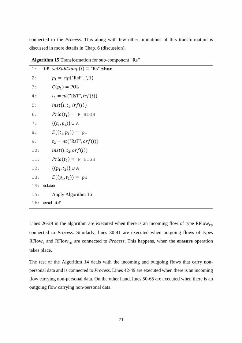
71
connected to the Process. This along with few other limitations of this transformation is
discussed in more details in Chap. 6 (discussion).
Algorithm 15 Transformation for sub-component “Rs”
1: if 𝑠𝑒𝑙𝑆𝑢𝑏𝐶𝑜𝑚𝑝(𝑖) ≡ "Rs" then
2: 𝑝1 = 𝑛𝑝("RsP", 𝑖, 1)
3: 𝐶(𝑝1) = POL
4: 𝑡1 = 𝑛𝑡("RsT", 𝑖𝑟𝑓(𝑖))
5: 𝑖𝑛𝑠𝑡(𝑖, 𝑡1, 𝑖𝑟𝑓(𝑖))
6: 𝑃𝑟𝑖𝑜(𝑡1) = P_HIGH
7: {(𝑡1, 𝑝1)} ∪ 𝐴
8: 𝐸((𝑡1, 𝑝1)) = p1
9: 𝑡2 = 𝑛𝑡("RsT", 𝑜𝑟𝑓(𝑖))
10: 𝑖𝑛𝑠𝑡(𝑖, 𝑡2, 𝑜𝑟𝑓(𝑖))
11: 𝑃𝑟𝑖𝑜(𝑡2) = P_HIGH
12: {(𝑝1, 𝑡2)} ∪ 𝐴
13: 𝐸((𝑝1, 𝑡2)) = p1
14: else
15: Apply Algorithm 16
16: end if
Lines 26-29 in the algorithm are executed when there is an incoming flow of type RFlowrp
connected to Process. Similarly, lines 30-41 are executed when outgoing flows of types
RFlowr and RFlowrp are connected to Process. This happens, when the erasure operation
takes place.
The rest of the Algorithm 14 deals with the incoming and outgoing flows that carry non-
personal data and is connected to Process. Lines 42-49 are executed when there is an incoming
flow carrying non-personal data. On the other hand, lines 50-65 are executed when there is an
outgoing flow carrying non-personal data.
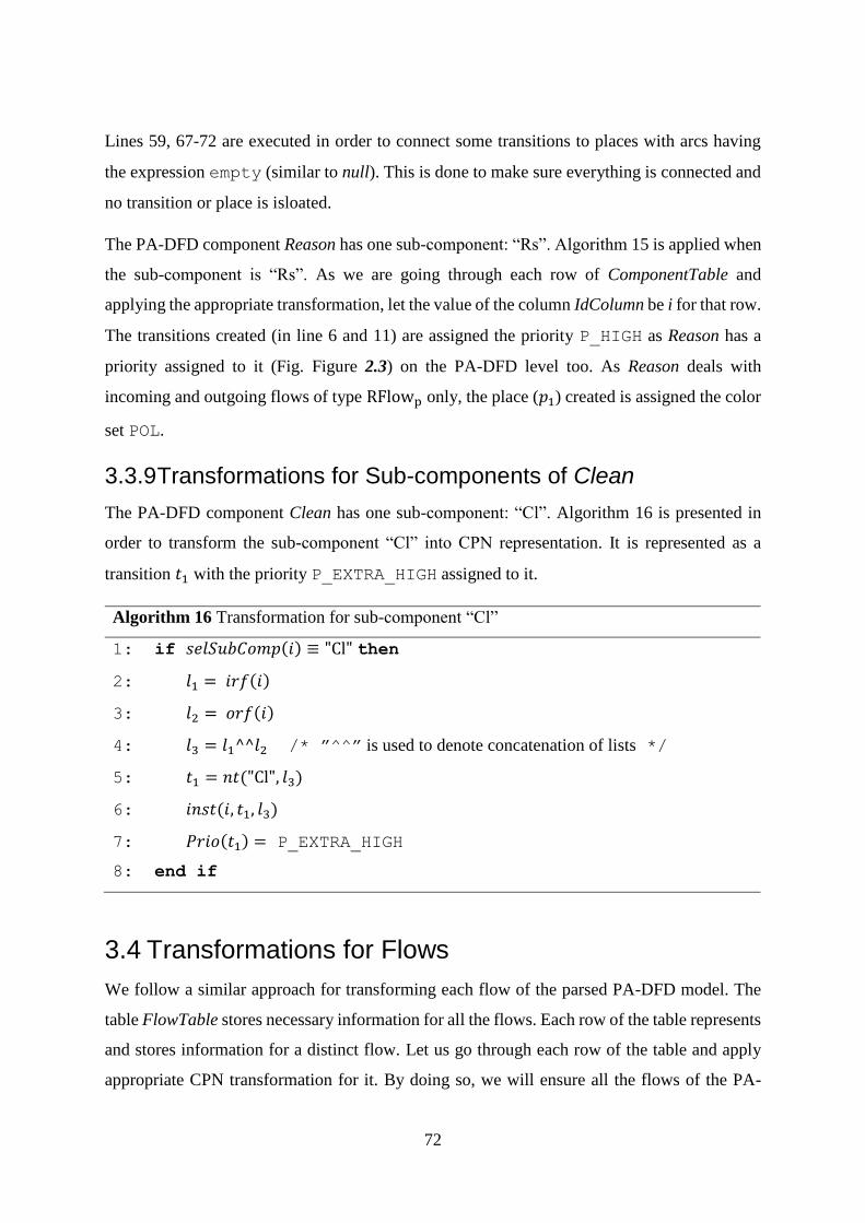
72
Lines 59, 67-72 are executed in order to connect some transitions to places with arcs having
the expression empty (similar to null). This is done to make sure everything is connected and
no transition or place is isloated.
The PA-DFD component Reason has one sub-component: “Rs”. Algorithm 15 is applied when
the sub-component is “Rs”. As we are going through each row of ComponentTable and
applying the appropriate transformation, let the value of the column IdColumn be i for that row.
The transitions created (in line 6 and 11) are assigned the priority P_HIGH as Reason has a
priority assigned to it (Fig. Figure 2.3) on the PA-DFD level too. As Reason deals with
incoming and outgoing flows of type RFlowp only, the place (𝑝1) created is assigned the color
set POL.
3.3.9 Transformations for Sub-components of Clean
The PA-DFD component Clean has one sub-component: “Cl”. Algorithm 16 is presented in
order to transform the sub-component “Cl” into CPN representation. It is represented as a
transition 𝑡1 with the priority P_EXTRA_HIGH assigned to it.
Algorithm 16 Transformation for sub-component “Cl”
1: if 𝑠𝑒𝑙𝑆𝑢𝑏𝐶𝑜𝑚𝑝(𝑖) ≡ "Cl" then
2: 𝑙1 = 𝑖𝑟𝑓(𝑖)
3: 𝑙2 = 𝑜𝑟𝑓(𝑖)
4: 𝑙3 = 𝑙1^^𝑙2 /* ”^^” is used to denote concatenation of lists */
5: 𝑡1 = 𝑛𝑡("Cl", 𝑙3)
6: 𝑖𝑛𝑠𝑡(𝑖, 𝑡1, 𝑙3)
7: 𝑃𝑟𝑖𝑜(𝑡1) = P_EXTRA_HIGH
8: end if
3.4 Transformations for Flows
We follow a similar approach for transforming each flow of the parsed PA-DFD model. The
table FlowTable stores necessary information for all the flows. Each row of the table represents
and stores information for a distinct flow. Let us go through each row of the table and apply
appropriate CPN transformation for it. By doing so, we will ensure all the flows of the PA-
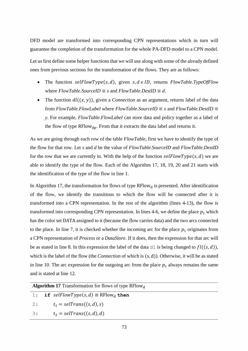
73
DFD model are transformed into corresponding CPN representations which in turn will
guarantee the completion of the transformation for the whole PA-DFD model to a CPN model.
Let us first define some helper functions that we will use along with some of the already defined
ones from previous sections for the transformation of the flows. They are as follows:
The function 𝑠𝑒𝑙𝐹𝑙𝑜𝑤𝑇𝑦𝑝𝑒(𝑠, 𝑑), given 𝑠, 𝑑 𝜖 𝐼𝐷, returns FlowTable.TypeOfFlow
where FlowTable.SourceID ≡ s and FlowTable.DestID ≡ d.
The function 𝑑𝑙((𝑥, 𝑦)), given a Connection as an argument, returns label of the data
from FlowTable.FlowLabel where FlowTable.SourceID ≡ x and FlowTable.DestID ≡
y. For example, FlowTable.FlowLabel can store data and policy together as a label of
the flow of type RFlowdp. From that it extracts the data label and returns it.
As we are going through each row of the table FlowTable, first we have to identify the type of
the flow for that row. Let s and d be the value of FlowTable.SourceID and FlowTable.DestID
for the row that we are currently in. With the help of the function 𝑠𝑒𝑙𝐹𝑙𝑜𝑤𝑇𝑦𝑝𝑒(𝑠, 𝑑) we are
able to identify the type of the flow. Each of the Algorithm 17, 18, 19, 20 and 21 starts with
the identification of the type of the flow in line 1.
In Algorithm 17, the transformation for flows of type RFlowd is presented. After identification
of the flow, we identify the transitions to which the flow will be connected after it is
transformed into a CPN representation. In the rest of the algorithm (lines 4-13), the flow is
transformed into corresponding CPN representation. In lines 4-6, we define the place 𝑝1 which
has the color set DATA assigned to it (because the flow carries data) and the two arcs connected
to the place. In line 7, it is checked whether the incoming arc for the place 𝑝1 originates from
a CPN representation of Process or a DataStore. If it does, then the expression for that arc will
be as stated in line 8. In this expression the label of the data d1 is being changed to 𝑓𝑙((𝑠, 𝑑)),
which is the label of the flow (the Connection of which is (s, d)). Otherwise, it will be as stated
in line 10. The arc expression for the outgoing arc from the place 𝑝1 always remains the same
and is stated at line 12.
Algorithm 17 Transformation for flows of type RFlowd
1: if 𝑠𝑒𝑙𝐹𝑙𝑜𝑤𝑇𝑦𝑝𝑒(𝑠, 𝑑) ≡ RFlowd then
2: 𝑡1 = 𝑠𝑒𝑙𝑇𝑟𝑎𝑛𝑠((𝑠, 𝑑), 𝑠)
3: 𝑡2 = 𝑠𝑒𝑙𝑇𝑟𝑎𝑛𝑠((𝑠, 𝑑), 𝑑)
74
4: 𝑝1 = 𝑛𝑝("DP", 𝑠, 𝑑) /* “DP” for ‘D’ata ‘P’lace. The place for tokens of color
set DATA */
5: 𝐶(𝑝1) = DATA
6: {(𝑡1, 𝑝1), (𝑝1, 𝑡2)} ∪ A
7: if 𝑠𝑒𝑙𝑆𝑢𝑏𝐶𝑜𝑚𝑝(𝑠) ≡ ("Pr" 𝐨𝐫 "DSG" 𝐨𝐫 "DSE") then
8: E((𝑡1, 𝑝1)) =dataLab(d1,𝑓𝑙((𝑠, 𝑑)))
9: else
10: E((𝑡1, 𝑝1)) = d1
11: end if
12: E((𝑝1, 𝑡2)) = d1
13: else
14: Apply Algorithm 18
15: end if
Algorithm 18 states the transformation for flows of type RFlowp. It is almost similar to
Algorithm 17. The only differences are, the color set assigned to the place 𝑝1 is POL (because
the flow carries policy) and both the incoming and outgoing arcs for the place have the same
expression (line 7).
Algorithm 18 Transformation for flows of type RFlowp
1: if 𝑠𝑒𝑙𝐹𝑙𝑜𝑤𝑇𝑦𝑝𝑒(𝑠, 𝑑) ≡ RFlowp then
2: 𝑡1 = 𝑠𝑒𝑙𝑇𝑟𝑎𝑛𝑠((𝑠, 𝑑), 𝑠)
3: 𝑡2 = 𝑠𝑒𝑙𝑇𝑟𝑎𝑛𝑠((𝑠, 𝑑), 𝑑)
4: 𝑝1 = 𝑛𝑝("PP", 𝑠, 𝑑) /* “PP” for ‘P’olicy ‘P’lace. The place for tokens of color
set POL */
5: 𝐶(𝑝1) = POL
6: {(𝑡1, 𝑝1), (𝑝1, 𝑡2)} ∪ A
7: E(𝑎) = p1 where, 𝑎 𝜖 {(𝑡1, 𝑝1), (𝑝1, 𝑡2)}
8: else
9: Apply Algorithm 19
10: end if
75
Algorithm 19 is almost identical to Algorithm 17, except it is for the flows who have type
RFlowdp (i.e., flows that carry personal data and policy together as a tuple). Understandably,
the place 𝑝1, in this case, needs to have the color set DATAxPOL assigned to it in order to
accommodate the tokens of the same color set. The incoming arc to the place can have one of
two different expressions. In line 7 it is checked whether the incoming arc to the place 𝑝1
originates from the CPN representation of a Process. If that is the case, then the expression will
be as it is stated in line 7 (where, after changing the label of the data d1 to the label of the flow,
the function processData is applied, which adds to the PR_HISTORY of d1 the name of
the Process the arc originates from). Otherwise, the expression for the incoming arc to 𝑝1 will
be as stated in line 10. The outgoing arc from 𝑝1 always has the same expression and is stated
in line 12.
Algorithm 19 Transformation for flows of type RFlowdp
1: if 𝑠𝑒𝑙𝐹𝑙𝑜𝑤𝑇𝑦𝑝𝑒(𝑠, 𝑑) ≡ RFlowdp then
2: 𝑡1 = 𝑠𝑒𝑙𝑇𝑟𝑎𝑛𝑠((𝑠, 𝑑), 𝑠)
3: 𝑡2 = 𝑠𝑒𝑙𝑇𝑟𝑎𝑛𝑠((𝑠, 𝑑), 𝑑)
4: 𝑝1 = 𝑛𝑝("DPP", 𝑠, 𝑑) /* “DPP” for ‘D’ata and ‘P’olicy ‘P’lace. The place for
tokens of color set DATAxPOL */
5: 𝐶(𝑝1) = DATAxPOL
6: {(𝑡1, 𝑝1), (𝑝1, 𝑡2)} ∪ A
7: if 𝑠𝑒𝑙𝑆𝑢𝑏𝐶𝑜𝑚𝑝(𝑠) ≡ "Pr" then
8: E((𝑡1, 𝑝1)) = (processData(dataLab(d1,𝑑𝑙((𝑠, 𝑑))),
𝐶𝑜𝑛𝑇𝑜(𝑑, (𝑠, 𝑑), Process)),p1)
9: else
10: E((𝑡1, 𝑝1)) = (d1,p1)
11: end if
12: E((𝑝1, 𝑡2)) = (d1,p1)
13: else
14: Apply Algorithm 20
15: end if
76
Algorithm 20 states the transformation for flows of type RFlowr and DFlowr. It is almost
identical to Algorithm 18. Few differences include, the color set assigned to the place 𝑝1 is REF
(because the flow carries reference to certain data) and both the incoming and outgoing arcs
for the place have the same expression, id (except when the incoming arc’s source is Clean).
Algorithm 20 Transformation for flows of type RFlowr and DFlowr
1: if 𝑠𝑒𝑙𝐹𝑙𝑜𝑤𝑇𝑦𝑝𝑒(𝑠, 𝑑) ≡ (RFlowr 𝐨𝐫 DFlowr) then
2: 𝑡1 = 𝑠𝑒𝑙𝑇𝑟𝑎𝑛𝑠((𝑠, 𝑑), 𝑠)
3: 𝑡2 = 𝑠𝑒𝑙𝑇𝑟𝑎𝑛𝑠((𝑠, 𝑑), 𝑑)
4: 𝑝1 = 𝑛𝑝("RP", 𝑠, 𝑑) /* “RP” for ‘R’eference ‘P’lace. The place for tokens of
color set REF
5: 𝐶(𝑝1) = REF
6: {(𝑡1, 𝑝1), (𝑝1, 𝑡2)} ∪ A
7: if 𝑐𝑜𝑛𝑊𝑖𝑡ℎ([(𝑠, 𝑑)], 𝐶𝑙𝑒𝑎𝑛) ≡ [(𝑠, 𝑑)] then
8: 𝐸(𝑡1, 𝑝1) = #1p1
9: else
10: 𝐸(𝑡1, 𝑝1) = id
11: end if
12: E((𝑝1, 𝑡2)) = id
13: else
14: Apply Algorithm 21
15: end if
In Algorithm 21 we present the transformation for flows of type RFlowrp. Again, it is almost
identical to Algorithm 18. The only differences are, the color set assigned to the place 𝑝1 is
REFxPOL (because the flow carries reference to certain data and a policy together as a tuple)
and both the incoming and outgoing arcs for the place 𝑝1 have the same expression (line 7).
Algorithm 21 Transformation for flows of type RFlowrp
1: if 𝑠𝑒𝑙𝐹𝑙𝑜𝑤𝑇𝑦𝑝𝑒(𝑠, 𝑑) ≡ RFlowrp then
77
2: 𝑡1 = 𝑠𝑒𝑙𝑇𝑟𝑎𝑛𝑠((𝑠, 𝑑), 𝑠)
3: 𝑡2 = 𝑠𝑒𝑙𝑇𝑟𝑎𝑛𝑠((𝑠, 𝑑), 𝑑)
4: 𝑝1 = 𝑛𝑝("RPP", 𝑠, 𝑑) /* “RPP” for ‘R’eference ‘P’olicy ‘P’lace. The place
for tokens of color set REFxPOL
5: 𝐶(𝑝1) = REFxPOL
6: {(𝑡1, 𝑝1), (𝑝1, 𝑡2)} ∪ A
7: E((𝑡1, 𝑝1), (𝑝1, 𝑡2)) = (id,p)
8: end if
After all the components and flows of the PA-DFD model are transformed, we get a Colored
Petri Net represented by the nine-tuple (𝑃, 𝑇, 𝐴, ∑, 𝑉, 𝐶, 𝐺, 𝐸, 𝐼). However, we do not yet use
the initialization function 𝐼 (to initialize places with tokens) in the transformation. As tokens
will be used to represent information, we need to initialize them (in places of the CPN model)
at the time of verification.
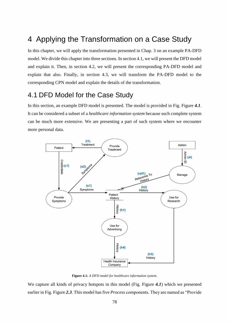
78
4 Applying the Transformation on a Case Study
In this chapter, we will apply the transformation presented in Chap. 3 on an example PA-DFD
model. We divide this chapter into three sections. In section 4.1, we will present the DFD model
and explain it. Then, in section 4.2, we will present the corresponding PA-DFD model and
explain that also. Finally, in section 4.3, we will transform the PA-DFD model to the
corresponding CPN model and explain the details of the transformation.
4.1 DFD Model for the Case Study
In this section, an example DFD model is presented. The model is provided in Fig. Figure 4.1.
It can be considered a subset of a healthcare information system because such complete system
can be much more extensive. We are presenting a part of such system where we encounter
more personal data.
Figure 4.1: A DFD model for healthcare information system.
We capture all kinds of privacy hotspots in this model (Fig. Figure 4.1) which we presented
earlier in Fig. Figure 2.3. This model has five Process components. They are named as “Provide
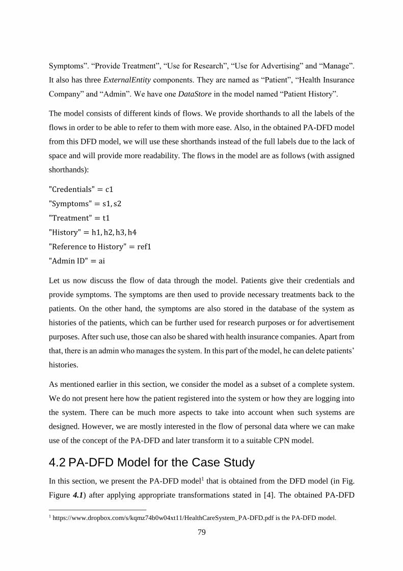
79
Symptoms”. “Provide Treatment”, “Use for Research”, “Use for Advertising” and “Manage”.
It also has three ExternalEntity components. They are named as “Patient”, “Health Insurance
Company” and “Admin”. We have one DataStore in the model named “Patient History”.
The model consists of different kinds of flows. We provide shorthands to all the labels of the
flows in order to be able to refer to them with more ease. Also, in the obtained PA-DFD model
from this DFD model, we will use these shorthands instead of the full labels due to the lack of
space and will provide more readability. The flows in the model are as follows (with assigned
shorthands):
"Credentials" = c1
"Symptoms" = s1, s2
"Treatment" = t1
"History" = h1, h2, h3, h4
"Reference to History" = ref1
"Admin ID" = ai
Let us now discuss the flow of data through the model. Patients give their credentials and
provide symptoms. The symptoms are then used to provide necessary treatments back to the
patients. On the other hand, the symptoms are also stored in the database of the system as
histories of the patients, which can be further used for research purposes or for advertisement
purposes. After such use, those can also be shared with health insurance companies. Apart from
that, there is an admin who manages the system. In this part of the model, he can delete patients’
histories.
As mentioned earlier in this section, we consider the model as a subset of a complete system.
We do not present here how the patient registered into the system or how they are logging into
the system. There can be much more aspects to take into account when such systems are
designed. However, we are mostly interested in the flow of personal data where we can make
use of the concept of the PA-DFD and later transform it to a suitable CPN model.
4.2 PA-DFD Model for the Case Study
In this section, we present the PA-DFD model1 that is obtained from the DFD model (in Fig.
Figure 4.1) after applying appropriate transformations stated in [4]. The obtained PA-DFD
1 https://www.dropbox.com/s/kqmz74b0w04xt11/HealthCareSystem_PA-DFD.pdf is the PA-DFD model.
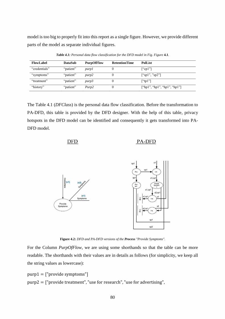
80
model is too big to properly fit into this report as a single figure. However, we provide different
parts of the model as separate individual figures.
Table 4.1: Personal data flow classification for the DFD model in Fig. Figure 4.1.
FlowLabel DataSub PurpOfFlow RetentionTime PolList
“credentials” “patient” purp1 0 [“cp1”]
“symptoms” “patient” purp2 0 [“sp1”, ”sp2”]
“treatment” “patient” purp3 0 [“tp1”]
“history” “patient” Purp2 0 [“hp1”, “hp1”, “hp1”, “hp1”]
The Table 4.1 (DFClass) is the personal data flow classification. Before the transformation to
PA-DFD, this table is provided by the DFD designer. With the help of this table, privacy
hotspots in the DFD model can be identified and consequently it gets transformed into PA-
DFD model.
Figure 4.2: DFD and PA-DFD versions of the Process "Provide Symptoms".
For the Column PurpOfFlow, we are using some shorthands so that the table can be more
readable. The shorthands with their values are in details as follows (for simplicity, we keep all
the string values as lowercase):
purp1 = ["provide symptoms"]
purp2 = ["provide treatment", "use for research", "use for advertising",
81
"health insurance company"]
purp3 = ["patient"]
The column RetentionTime is given the value 0 for all of its rows because we are not
considering the notion of time for the transformation. Here, 0 can be interpreted as infinite
retention time.
The table has another column named PolList. We add this column and its values after the PA-
DFD transformation is made. This column stores the list of labels of the policy flows in the
PA-DFD model for corresponding personal data in the row. This column is particularly
important at the time of the transformation of the PA-DFD model to CPN model.
Figure 4.3: DFD and PA-DFD versions of the DataStore "Patient History".
Two different parts of PA-DFD model are presented as separate figures with their
corresponding DFD parts. In Fig. 4.2, we present the Process “Provide Symptoms”. Here, on
the PA-DFD level, the Limit and Request (written in short as “Lim” and “Req”) receive the
data c1 and its corresponding policy cp1 respectively. The process “provide symptoms” takes
as an input the tuple (c1, cp1). Then, the data s1 and s2 are produced and forwarded to the rest
of the model with their corresponding policies sp1 and sp2 after necessary information
regarding the data c1 is logged.
Similarly, In Fig. 4.3, we present the DataStore “Patient History” (with only the recording
part on the PA-DFD level). Here, Limit and Request receive the data s1 and its corresponding
policy sp1. Then, necessary information about them are logged before being stored in the
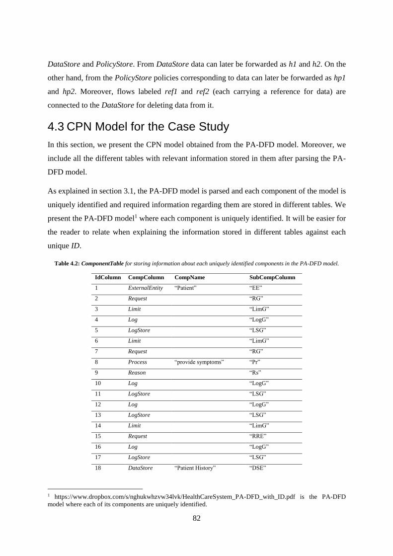
82
DataStore and PolicyStore. From DataStore data can later be forwarded as h1 and h2. On the
other hand, from the PolicyStore policies corresponding to data can later be forwarded as hp1
and hp2. Moreover, flows labeled ref1 and ref2 (each carrying a reference for data) are
connected to the DataStore for deleting data from it.
4.3 CPN Model for the Case Study
In this section, we present the CPN model obtained from the PA-DFD model. Moreover, we
include all the different tables with relevant information stored in them after parsing the PA-
DFD model.
As explained in section 3.1, the PA-DFD model is parsed and each component of the model is
uniquely identified and required information regarding them are stored in different tables. We
present the PA-DFD model1 where each component is uniquely identified. It will be easier for
the reader to relate when explaining the information stored in different tables against each
unique ID.
Table 4.2: ComponentTable for storing information about each uniquely identified components in the PA-DFD model.
IdColumn CompColumn CompName SubCompColumn
1 ExternalEntity “Patient” “EE”
2 Request “RG”
3 Limit “LimG”
4 Log “LogG”
5 LogStore “LSG”
6 Limit “LimG”
7 Request “RG”
8 Process “provide symptoms” “Pr”
9 Reason “Rs”
10 Log “LogG”
11 LogStore “LSG”
12 Log “LogG”
13 LogStore “LSG”
14 Limit “LimG”
15 Request “RRE”
16 Log “LogG”
17 LogStore “LSG”
18 DataStore “Patient History” “DSE”
1 https://www.dropbox.com/s/nghukwhzvw34lvk/HealthCareSystem_PA-DFD_with_ID.pdf is the PA-DFD
model where each of its components are uniquely identified.
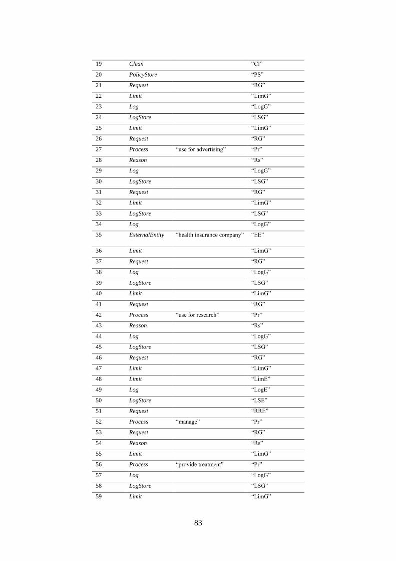
83
19 Clean “Cl”
20 PolicyStore “PS”
21 Request “RG”
22 Limit “LimG”
23 Log “LogG”
24 LogStore “LSG”
25 Limit “LimG”
26 Request “RG”
27 Process “use for advertising” “Pr”
28 Reason “Rs”
29 Log “LogG”
30 LogStore “LSG”
31 Request “RG”
32 Limit “LimG”
33 LogStore “LSG”
34 Log “LogG”
35 ExternalEntity “health insurance company” “EE”
36 Limit “LimG”
37 Request “RG”
38 Log “LogG”
39 LogStore “LSG”
40 Limit “LimG”
41 Request “RG”
42 Process “use for research” “Pr”
43 Reason “Rs”
44 Log “LogG”
45 LogStore “LSG”
46 Request “RG”
47 Limit “LimG”
48 Limit “LimE”
49 Log “LogE”
50 LogStore “LSE”
51 Request “RRE”
52 Process “manage” “Pr”
53 Request “RG”
54 Reason “Rs”
55 Limit “LimG”
56 Process “provide treatment” “Pr”
57 Log “LogG”
58 LogStore “LSG”
59 Limit “LimG”
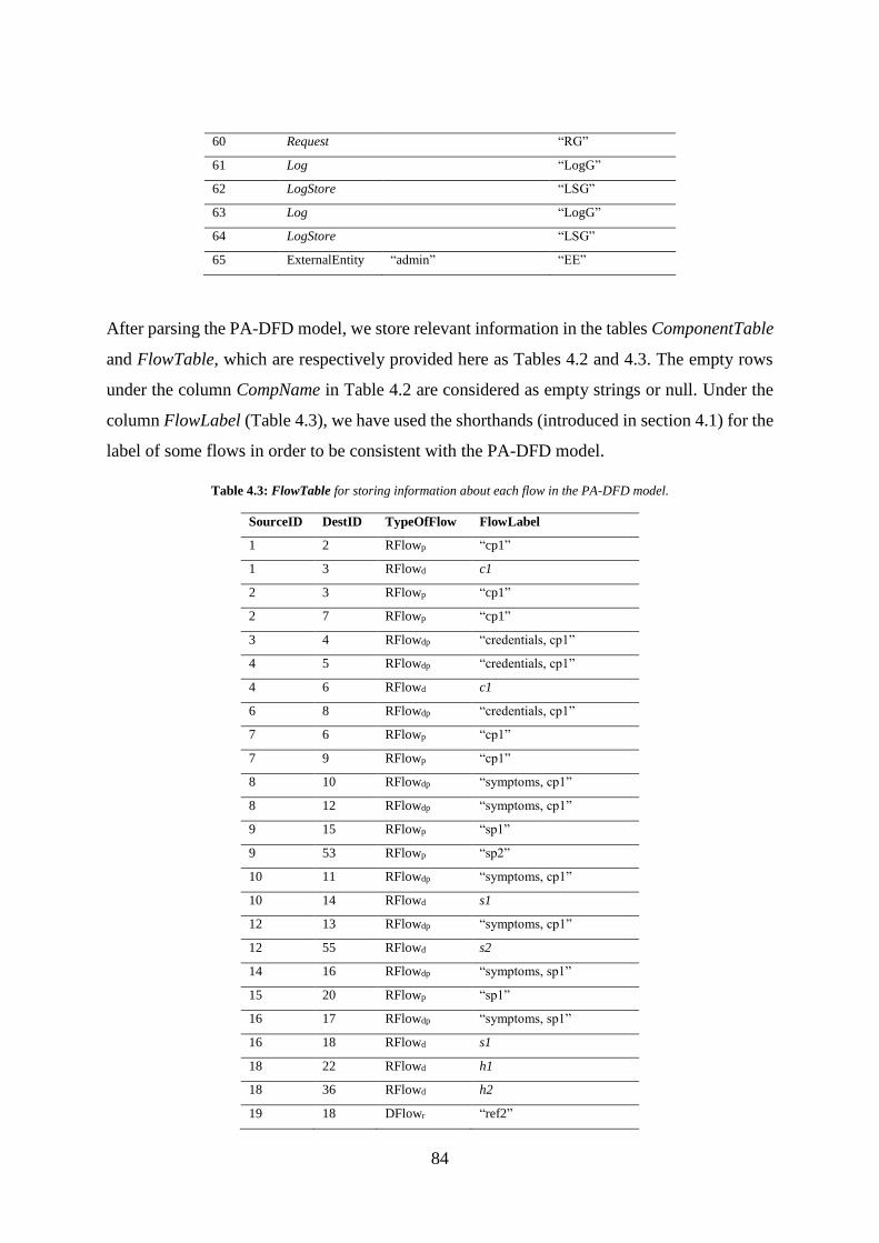
84
60 Request “RG”
61 Log “LogG”
62 LogStore “LSG”
63 Log “LogG”
64 LogStore “LSG”
65 ExternalEntity “admin” “EE”
After parsing the PA-DFD model, we store relevant information in the tables ComponentTable
and FlowTable, which are respectively provided here as Tables 4.2 and 4.3. The empty rows
under the column CompName in Table 4.2 are considered as empty strings or null. Under the
column FlowLabel (Table 4.3), we have used the shorthands (introduced in section 4.1) for the
label of some flows in order to be consistent with the PA-DFD model.
Table 4.3: FlowTable for storing information about each flow in the PA-DFD model.
SourceID DestID TypeOfFlow FlowLabel
1 2 RFlowp “cp1”
1 3 RFlowd c1
2 3 RFlowp “cp1”
2 7 RFlowp “cp1”
3 4 RFlowdp “credentials, cp1”
4 5 RFlowdp “credentials, cp1”
4 6 RFlowd c1
6 8 RFlowdp “credentials, cp1”
7 6 RFlowp “cp1”
7 9 RFlowp “cp1”
8 10 RFlowdp “symptoms, cp1”
8 12 RFlowdp “symptoms, cp1”
9 15 RFlowp “sp1”
9 53 RFlowp “sp2”
10 11 RFlowdp “symptoms, cp1”
10 14 RFlowd s1
12 13 RFlowdp “symptoms, cp1”
12 55 RFlowd s2
14 16 RFlowdp “symptoms, sp1”
15 20 RFlowp “sp1”
16 17 RFlowdp “symptoms, sp1”
16 18 RFlowd s1
18 22 RFlowd h1
18 36 RFlowd h2
19 18 DFlowr “ref2”
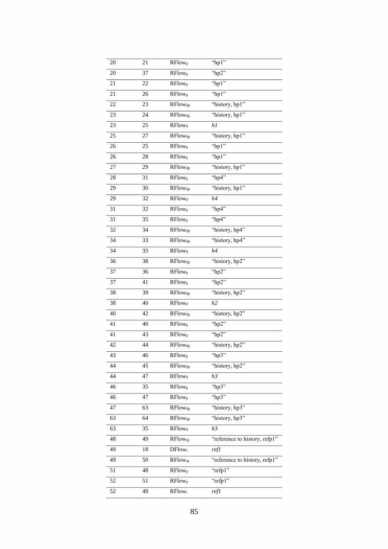
85
20 21 RFlowp “hp1”
20 37 RFlowp “hp2”
21 22 RFlowp “hp1”
21 26 RFlowp “hp1”
22 23 RFlowdp “history, hp1”
23 24 RFlowdp “history, hp1”
23 25 RFlowd h1
25 27 RFlowdp “history, hp1”
26 25 RFlowp “hp1”
26 28 RFlowp “hp1”
27 29 RFlowdp “history, hp1”
28 31 RFlowp “hp4”
29 30 RFlowdp “history, hp1”
29 32 RFlowd h4
31 32 RFlowp “hp4”
31 35 RFlowp “hp4”
32 34 RFlowdp “history, hp4”
34 33 RFlowdp “history, hp4”
34 35 RFlowd h4
36 38 RFlowdp “history, hp2”
37 36 RFlowp “hp2”
37 41 RFlowp “hp2”
38 39 RFlowdp “history, hp2”
38 40 RFlowd h2
40 42 RFlowdp “history, hp2”
41 40 RFlowp “hp2”
41 43 RFlowp “hp2”
42 44 RFlowdp “history, hp2”
43 46 RFlowp “hp3”
44 45 RFlowdp “history, hp2”
44 47 RFlowd h3
46 35 RFlowp “hp3”
46 47 RFlowp “hp3”
47 63 RFlowdp “history, hp3”
63 64 RFlowdp “history, hp3”
63 35 RFlowd h3
48 49 RFlowrp “reference to history, refp1”
49 18 DFlowr ref1
49 50 RFlowrp “reference to history, refp1”
51 48 RFlowp “refp1”
52 51 RFlowp “refp1”
52 48 RFlowr ref1
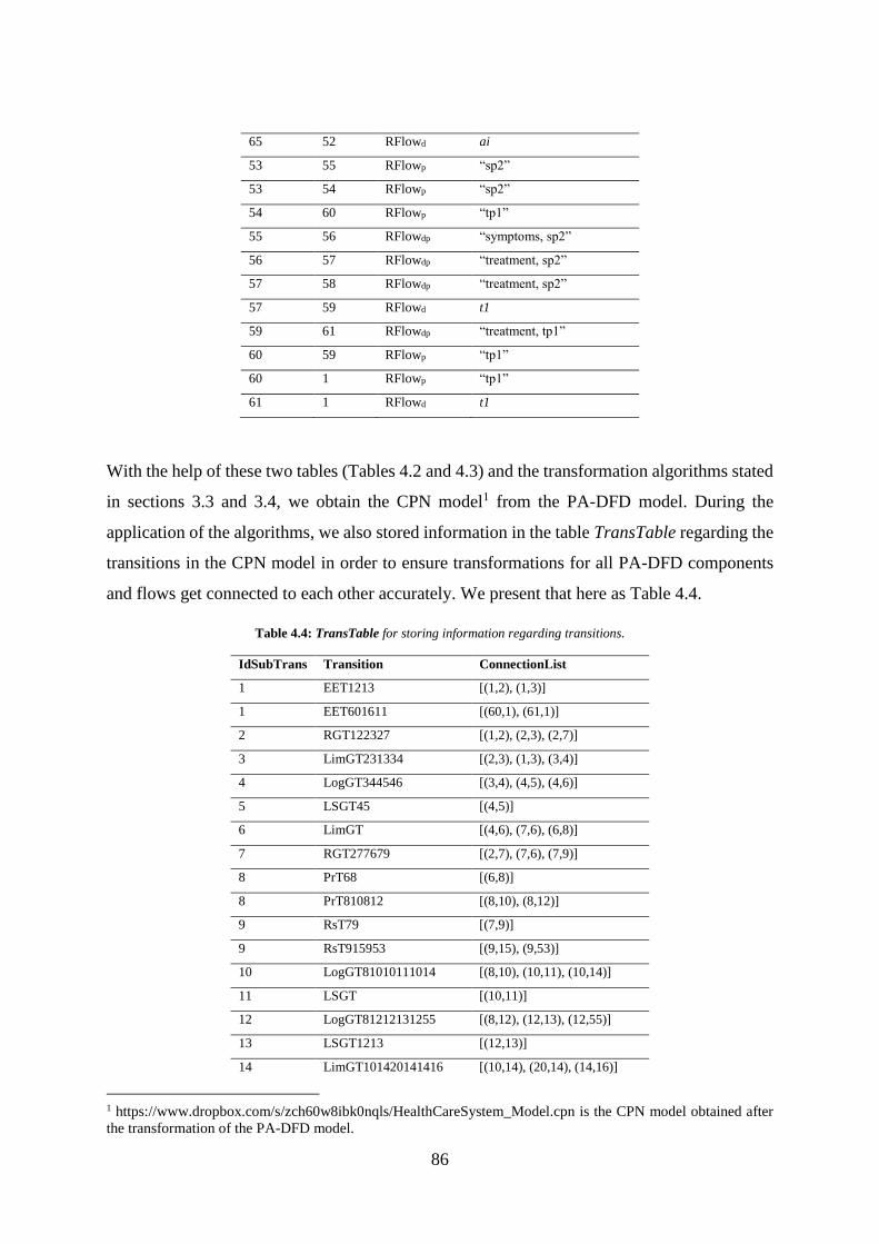
86
65 52 RFlowd ai
53 55 RFlowp “sp2”
53 54 RFlowp “sp2”
54 60 RFlowp “tp1”
55 56 RFlowdp “symptoms, sp2”
56 57 RFlowdp “treatment, sp2”
57 58 RFlowdp “treatment, sp2”
57 59 RFlowd t1
59 61 RFlowdp “treatment, tp1”
60 59 RFlowp “tp1”
60 1 RFlowp “tp1”
61 1 RFlowd t1
With the help of these two tables (Tables 4.2 and 4.3) and the transformation algorithms stated
in sections 3.3 and 3.4, we obtain the CPN model1 from the PA-DFD model. During the
application of the algorithms, we also stored information in the table TransTable regarding the
transitions in the CPN model in order to ensure transformations for all PA-DFD components
and flows get connected to each other accurately. We present that here as Table 4.4.
Table 4.4: TransTable for storing information regarding transitions.
IdSubTrans Transition ConnectionList
1 EET1213 [(1,2), (1,3)]
1 EET601611 [(60,1), (61,1)]
2 RGT122327 [(1,2), (2,3), (2,7)]
3 LimGT231334 [(2,3), (1,3), (3,4)]
4 LogGT344546 [(3,4), (4,5), (4,6)]
5 LSGT45 [(4,5)]
6 LimGT [(4,6), (7,6), (6,8)]
7 RGT277679 [(2,7), (7,6), (7,9)]
8 PrT68 [(6,8)]
8 PrT810812 [(8,10), (8,12)]
9 RsT79 [(7,9)]
9 RsT915953 [(9,15), (9,53)]
10 LogGT81010111014 [(8,10), (10,11), (10,14)]
11 LSGT [(10,11)]
12 LogGT81212131255 [(8,12), (12,13), (12,55)]
13 LSGT1213 [(12,13)]
14 LimGT101420141416 [(10,14), (20,14), (14,16)]
1 https://www.dropbox.com/s/zch60w8ibk0nqls/HealthCareSystem_Model.cpn is the CPN model obtained after
the transformation of the PA-DFD model.

87
15 RRET9151520 [(9,15), (15,20)]
16 LogGT [(14,16), (16,17), (16,18)]
17 LSGT1617 [(16,17)]
18 DSET1618 [(16,18)]
18 DSET1822 [(18,22)]
18 DSET1837 [(18,37)]
18 DSET1918 [(19,18)]
18 DSET4918 [(49,18)]
19 Cl20191918 [(20,19), (19,18)]
20 PST1520 [(15,20)]
20 PST2014 [(20,14)]
20 PST2021 [(20,21)]
20 PST2037 [(20,37)]
20 PST2019 [(20,19)]
21 RGT202121222126 [(20,21). (21,22), (21,26)]
22 LimGT182221222223 [(18,22), (21,22), (22,23)]
23 LogGT222323242325 [(22,23), (23,24), (23,25)]
24 LSGT2324 [(23,24)]
25 LimGT232526252527 [(23,25), (26,25), (25,27)]
26 RGT21262652628 [(21,26), (26,25), (26,28)]
27 PrT2527 [(25,27)]
27 PrT2729 [(27,29)]
28 RsT2628 [(26,28)]
28 RsT2831 [(28,31)]
29 LogGT272929302932 [(27,29), (29,30), (29,32)]
30 LSGT2930 [(29,30)]
31 RGT283131323135 [(28,31), (31,32), (31,35)]
32 LimGT313229323234 [(31,32), (29,32), (32,34)]
33 LSGT3433 [(34,33)]
34 LogGT323434333435 [(32,34), (34,33), (34,35)]
35 EET34353135 [(34,35), (31,35)]
36 LimGT183637363638 [(18,36), (37,36), (36,38)]
37 RGT203737363741 [(20,37), (37,26), (37,41)]
38 LogGT363838393840 [(36,38), (38,39), (38,40)]
39 LSGT3839 [(38,39)]
40 LimGT384041404042 [(38,40), (41,40), (40,42)]
41 RGT374141404143 [(37,41), (41,40), (41,43)]
42 PrT4042 [(40,42)]
42 PrT4244 [(42,44)]
43 RsT4143 [(41,43)]
43 RsT4346 [(43,46)]
44 LogGT [(42,44), (44,45), (44,47)]

88
45 LSGT4445 [(44,45)]
46 RGT434646474635 [(43,46), (46,47), (46,35)]
47 LimGT464744474763 [(46,47), (44,47), (47,63)]
48 LimET514852484849 [(51,48), (52,48), (48,49)]
49 LogET484949504918 [(48,49), (49,50), (49,18)]
50 LSET4950 [(49,50)]
51 RRET52515148 [(52,51), (51,48)]
52 PrT6552 [(65,52)]
52 PrT52485251 [(52,48),(52,51)]
53 RGT95353555354 [(9,53), (53,55), (53,54)]
54 RsT5354 [(53,54)]
54 RsT5460 [(54,60)]
55 LimGT125553555556 [(12,55), (53,55), (55,56)]
56 PrT5556 [(55,56)]
56 PrT5657 [(56,57)]
57 LogGT565757585759 [(56,57), (57,58), (57,59)]
58 LSGT5758 [(57,58)]
59 LimGT575960595961 [(57,59), (60,59), (59,61)]
60 RGT54606059601 [(54,60), (60,59), (60,1)]
61 LogGT59616162611 [(59,61), (61,62), (61,1)]
62 LSGT6162 [(61,62)]
63 LogGT476363646335 [(47,63), (63,64), (63,35)]
64 LSGT6364 [(63,64)]
65 EET6552 [(65,52)]
Due to the size of the CPN model, it is not feasible to include the full model in the report.
However, we give parts of the model for some corresponding parts of the PA-DFD model. In
Fig. 4.2 and 4.3, we presented something similar.
In Fig. 4.2, we presented a snippet of the Process “provide symptoms” from both the DFD and
PA-DFD models. In Fig. 4.4, we show the snippet of the same Process from the CPN model.
Here, the tuple of data (“credentials”) and policy is incoming to the process “provide
symptoms” via the transition PrT68. Then, the data gets processed and changed into
“symptoms” (in the meantime adding the current process name in the process history of the
data) while it is outputted via two arcs (in the DFD and PA-DFD figures outputted s two flows)
from the transition PrT810812. Afterward, they are forwarded to the CPN representations of
Log and LogStore.
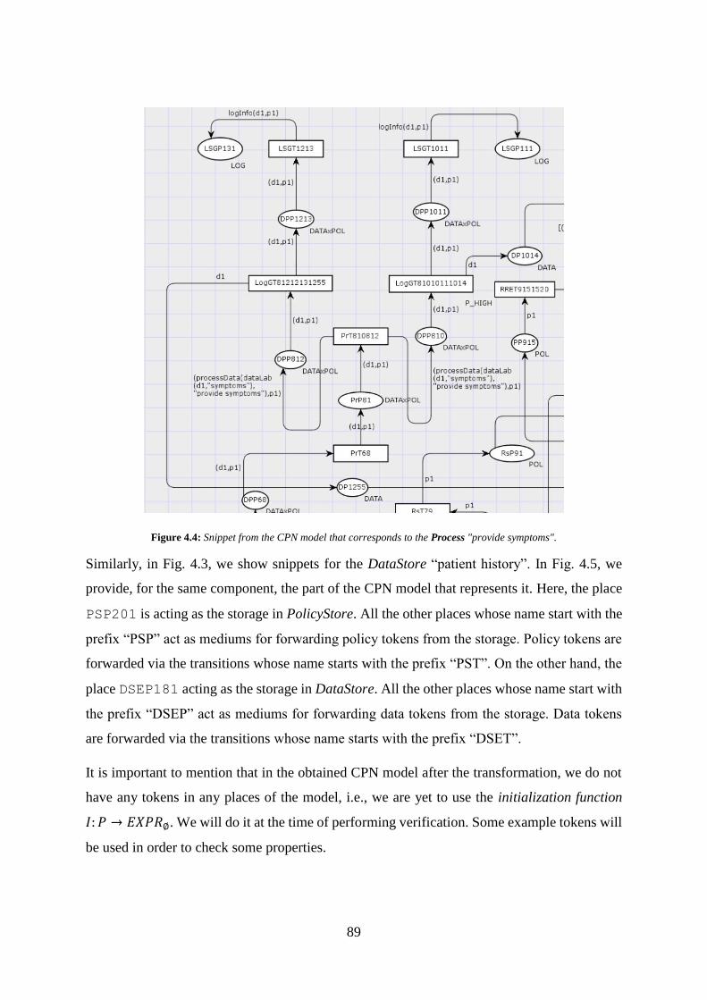
89
Figure 4.4: Snippet from the CPN model that corresponds to the Process "provide symptoms".
Similarly, in Fig. 4.3, we show snippets for the DataStore “patient history”. In Fig. 4.5, we
provide, for the same component, the part of the CPN model that represents it. Here, the place
PSP201 is acting as the storage in PolicyStore. All the other places whose name start with the
prefix “PSP” act as mediums for forwarding policy tokens from the storage. Policy tokens are
forwarded via the transitions whose name starts with the prefix “PST”. On the other hand, the
place DSEP181 acting as the storage in DataStore. All the other places whose name start with
the prefix “DSEP” act as mediums for forwarding data tokens from the storage. Data tokens
are forwarded via the transitions whose name starts with the prefix “DSET”.
It is important to mention that in the obtained CPN model after the transformation, we do not
have any tokens in any places of the model, i.e., we are yet to use the initialization function
𝐼: 𝑃 → 𝐸𝑋𝑃𝑅∅. We will do it at the time of performing verification. Some example tokens will
be used in order to check some properties.
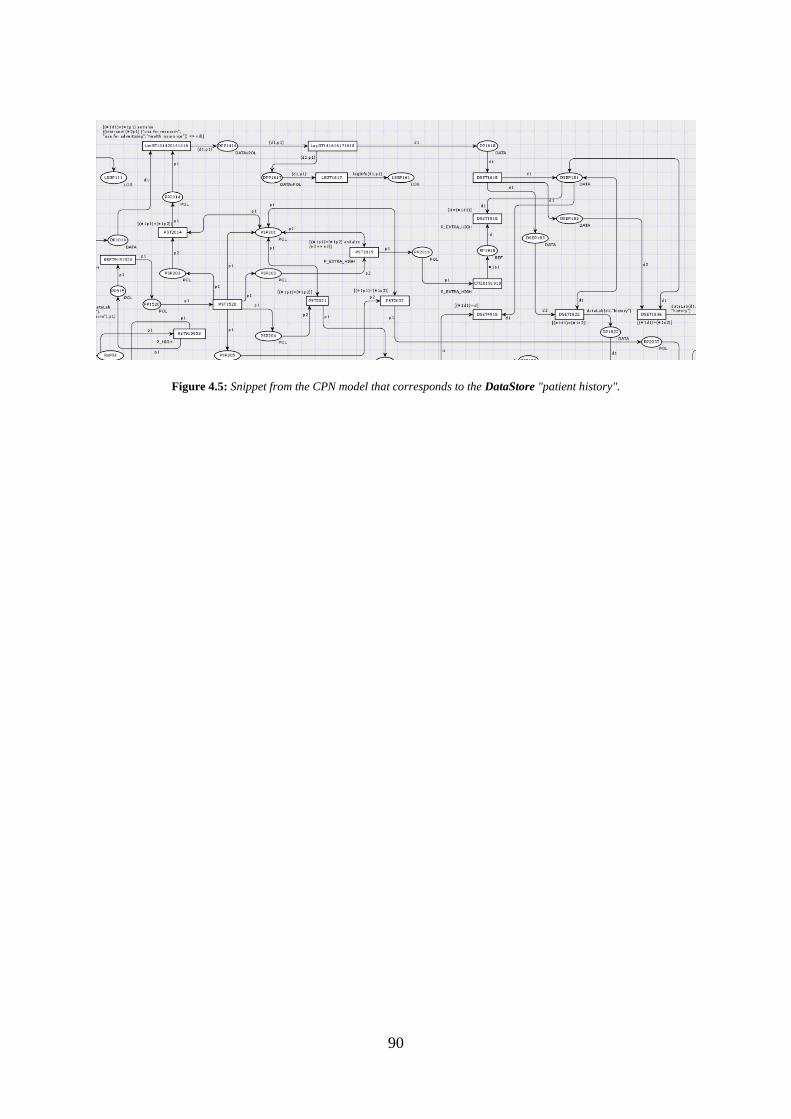
90
Figure 4.5: Snippet from the CPN model that corresponds to the DataStore "patient history".
91
5 Verification on the Obtained CPN Model from the
Case Study
In this chapter, we discuss the verification done in the CPN model from section 4.3. Properties
are checked in the model by means of CPN ML queries and using CPN Tools. Table 5.1
includes the privacy properties enforced at each hotspot (as mentioned in section 2.2) when a
DFD model is transformed to a PA-DFD model [4]. Taking these as a base, we check properties
in the CPN model obtained from the case study.
Table 5.1: Privacy properties applied to each hotspot [4].
Privacy properties
Purpose limitation. The collection of personal data is only allowed if the consent
for that data given by the data subject (external entity) covers the purpose of this
collection.
Accountability. The collection of personal data is allowed only if it the collection
is logged.
Right to change. Request can be made by the data subject at any given time to
change their current consent for what concerns the purpose of collection of their
personal data.
Purpose limitation. The disclosure of personal data is only allowed if the consent
for that data given by the data subject (external entity) covers the purpose of the
disclosure.
Accountability. The disclosure of personal data is allowed only if it this disclosure
is logged.
Policy propagation. Disclosure of personal data can only be made if the purpose
mentioned in the current consent (and retention time if applicable) for collection,
disclosure, usage, recording, retrieval, and erasure is propagated.
Right to change. Request can be made by the data subject at any given time to
change their current consent for what concerns the purpose of disclosure of their
personal data.
Purpose limitation. The usage of personal data is only allowed if the consent for
that data given by the data subject (external entity) covers the purpose of the usage.
Accountability. The usage of personal data is allowed only if it this usage is
logged.
Right to change. Request can be made by the data subject at any given time to
change their current consent for what concerns the purpose of usage of their
personal data.
Purpose limitation. The recording of personal data is only allowed if the consent
for that data given by the data subject (external entity) covers the purpose of the
recording.
Time retention. The recorded personal data can be in the system as long as the
current retention time given by the data subject has not expired.
Coll
ecti
on
D
iscl
osu
re
Usa
ge
Rec
ord
ing
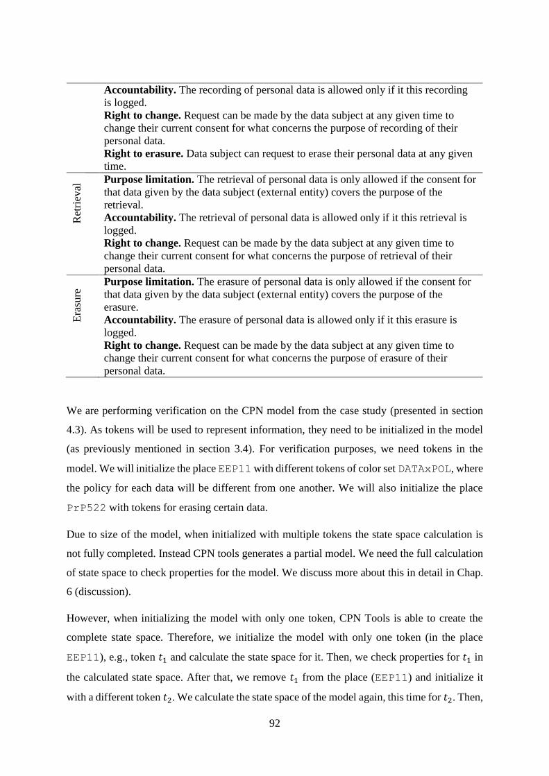
92
Accountability. The recording of personal data is allowed only if it this recording
is logged.
Right to change. Request can be made by the data subject at any given time to
change their current consent for what concerns the purpose of recording of their
personal data.
Right to erasure. Data subject can request to erase their personal data at any given
time.
Purpose limitation. The retrieval of personal data is only allowed if the consent for
that data given by the data subject (external entity) covers the purpose of the
retrieval.
Accountability. The retrieval of personal data is allowed only if it this retrieval is
logged.
Right to change. Request can be made by the data subject at any given time to
change their current consent for what concerns the purpose of retrieval of their
personal data.
Purpose limitation. The erasure of personal data is only allowed if the consent for
that data given by the data subject (external entity) covers the purpose of the
erasure.
Accountability. The erasure of personal data is allowed only if it this erasure is
logged.
Right to change. Request can be made by the data subject at any given time to
change their current consent for what concerns the purpose of erasure of their
personal data.
We are performing verification on the CPN model from the case study (presented in section
4.3). As tokens will be used to represent information, they need to be initialized in the model
(as previously mentioned in section 3.4). For verification purposes, we need tokens in the
model. We will initialize the place EEP11 with different tokens of color set DATAxPOL, where
the policy for each data will be different from one another. We will also initialize the place
PrP522 with tokens for erasing certain data.
Due to size of the model, when initialized with multiple tokens the state space calculation is
not fully completed. Instead CPN tools generates a partial model. We need the full calculation
of state space to check properties for the model. We discuss more about this in detail in Chap.
6 (discussion).
However, when initializing the model with only one token, CPN Tools is able to create the
complete state space. Therefore, we initialize the model with only one token (in the place
EEP11), e.g., token 𝑡1 and calculate the state space for it. Then, we check properties for 𝑡1 in
the calculated state space. After that, we remove 𝑡1 from the place (EEP11) and initialize it
with a different token 𝑡2. We calculate the state space of the model again, this time for 𝑡2. Then,
Ret
riev
al
Era
sure
93
we check properties for 𝑡2 in the calculated state space. We do this for five different tokens
whose policies are different from each other’s (allowing them to travel different parts of the
model). These tokens are listed as follows:
𝑡1 = 1`((1,"patient", "credentials", nil), (1, ["provide
symptoms", "provide treatment", "patient"]))
𝑡2 = 1`((2, "patient", "credentials", nil), (2, ["provide
symptoms", "provide treatment", "patient", "use for research"]))
𝑡3 = 1`((3, "patient", "credentials", nil), (3, ["provide
symptoms", "provide treatment", "patient", "use for research",
"erase"]))
𝑡4 = 1`((4, "patient", "credentials", nil), (4, ["provide
symptoms", "provide treatment", "patient", "use for
advertising"]))
𝑡5 = 1`((5, "patient", "credentials", nil), (5, ["provide
symptoms", "provide treatment", "patient", "use for
advertising", "health insurance company"]))
Logging of events are performed regarding the data that gets collected, disclosed, used,
recorded, retrieved or erased by means of LogStore. The obtained CPN model after the
transformation of the PA-DFD model represents each LogStore as a transition and a place that
are connected by an arc. Tokens in that place are relevant information of the data that are kept
in order to indicate logging of events. Therefore, for the different tokens stated above, places
that correspond to LogStore in the CPN model will store different information. By checking
these information in these places, we can ensure accountability. Furthermore, as logging of
events always takes place after the data had gone through Limit first, we can, therefore, ensure
successful purpose limitation.
For the purpose of checking properties with state space queries, we additionally define a color
set and two helper functions. They are provided as follows:
colset LOGs = list LOG;
fun LoggedOrNot(a1:LOGs, a2:REF)
= if (a1=nil) then false
else (if ((#1(hd a1))=a2) then true
94
else (LoggedOrNot((tl(a1)),a2)));
fun LoggedOk(a1:LOGs, a2:REF, a3:PR_HISTORY)
= if (a1=nil) then false
else (if ((#1(hd a1))=a2) then (contains (#4(hd a1)) a3)
else (LoggedOk((tl(a1)),a2,a3)));
The state space queries will make use of these aforementioned definitions in order to investigate
the state space. The color set LOGs is defined in order to access the multiset of a color set
(tokens in the places that has the color set LOG and correspond to LogStore). The function
LoggedOrNot, given a list of LOG (synonymous to multiset of LOG), and a2:REF, goes
through each element of the list and checks whether information regarding certain data with
the reference a2 was logged or not. The function LoggedOK, given a list of LOG, a2:REF,
and a3:PR_HITORY, goes through each element of the list and checks whether information
regarding certain data with the reference a2 includes the desired process history a3. If it does,
that confirms the data in question was processed by the processes whose names are in a3.
The places in the CPN model that correspond to LogStore are as follows:
LSGP51 corresponds to the LogStore with the ID 5 in the PA-DFD model. This
performs logging when the collection operation takes place.
LSGP621, LSGP331, and LSGP641 correspond to the LogStores with the ID 62, 33
and 64 respectively in the PA-DFD model. The first one performs logging when
disclosure operation happens to the ExternalEntity named “patient” and the last two
perform logging when disclosure operation happens to the ExternalEntity named
“health insurance company”.
LSGP131, LSGP111, LSGP581, LSGP301, and LSGP451 correspond to the
LogStores with the ID 13, 11, 58, 30 and 45 respectively in the PA-DFD model. The
first two perform logging when usage operation happens with the Process named
“provide symptoms”. The last three perform logging when usage operation happens
with the Processes named “provide treatment”, “use for advertising”, and “use for
research” respectively.
95
LSGP161 corresponds to the LogStore with the ID 16 in the PA-DFD model. It
performs logging when recording operation happens with the DataStore named
“patient history”.
LSGP391 and LSGP241 correspond to the LogStores with the ID 39 and 24 in the PA-
DFD model. Both of these perform logging when retrieval operation happens with the
DataStore named “patient history”.
LSGP501 corresponds to the LogStore with the ID 50 in the PA-DFD model. This
performs logging when the erasure operation takes place.
We do not check properties regarding erasure for the token 𝑡1, 𝑡2, 𝑡4 and 𝑡5 because we also
need to initialize a token in the place PrP522 in order to perform erasure operation (if the
policy corresponding the data allows). However, we do check it for the token 𝑡3 because when
we initialize the model with this token in the place EEP11, we will also add a token (which we
present later) to the place PrP522. For now, let us first initialize the model with the token 𝑡1
only, which can be denoted formally as follows:
𝐼(EEP11) = 𝑡1
Figure 5.1: State space queries for the model when it is initialized with token 𝑡1 only.
According to the policy provided in the token, its corresponding data can be collected from the
ExternalEntity “patient”, processed by the Processes “provide symptoms” and “provide
treatment”, and disclosed to the ExternalEntity “patient”. The policy does not cover necessary
consents for its corresponding data to get recorded in the DataStore “patient history” or get
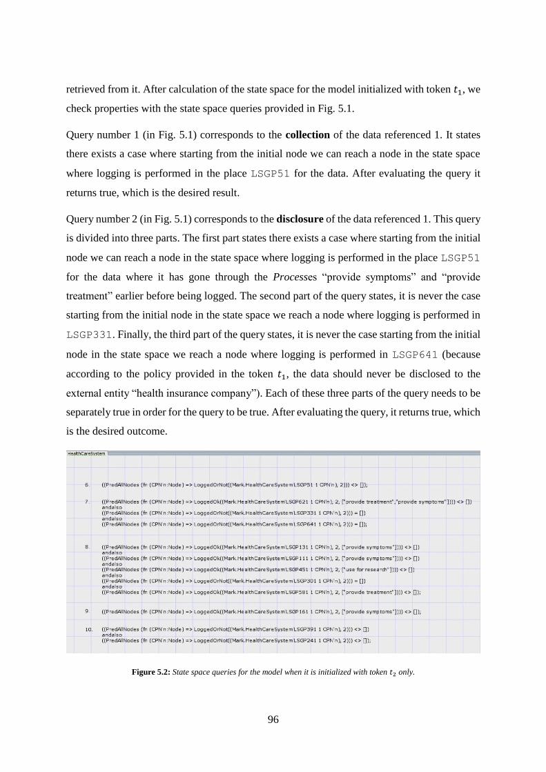
96
retrieved from it. After calculation of the state space for the model initialized with token 𝑡1, we
check properties with the state space queries provided in Fig. 5.1.
Query number 1 (in Fig. 5.1) corresponds to the collection of the data referenced 1. It states
there exists a case where starting from the initial node we can reach a node in the state space
where logging is performed in the place LSGP51 for the data. After evaluating the query it
returns true, which is the desired result.
Query number 2 (in Fig. 5.1) corresponds to the disclosure of the data referenced 1. This query
is divided into three parts. The first part states there exists a case where starting from the initial
node we can reach a node in the state space where logging is performed in the place LSGP51
for the data where it has gone through the Processes “provide symptoms” and “provide
treatment” earlier before being logged. The second part of the query states, it is never the case
starting from the initial node in the state space we reach a node where logging is performed in
LSGP331. Finally, the third part of the query states, it is never the case starting from the initial
node in the state space we reach a node where logging is performed in LSGP641 (because
according to the policy provided in the token 𝑡1, the data should never be disclosed to the
external entity “health insurance company”). Each of these three parts of the query needs to be
separately true in order for the query to be true. After evaluating the query, it returns true, which
is the desired outcome.
Figure 5.2: State space queries for the model when it is initialized with token 𝑡2 only.

97
Query number 3 (in Fig. 5.1) corresponds to the usage of the data referenced 1. The query is
divided into five parts where each of these parts needs to be true in order for the query to return
true. The first part states there exists a case starting from the initial node we can reach a node
in the state space where logging is performed in the place LSGP131 for the data where it has
gone through the Process “provide symptoms” before being logged. The second part is similar
to the first, except the logging happens in the place LSGP111. The third part states there exists
a case starting from the initial node we can reach a node in the state space where logging is
performed in the place LSGP581 for the data where it has gone through the Process “provide
treatment” before being logged. The fourth part of the query states, it is never the case starting
from the initial node in the state space we reach a node where logging is performed in
LSGP301 (because according to the policy provided in the token 𝑡1, the data should never be
used by the process “use for advertising”). Finally, the fifth part of the query states, it is never
the case starting from the initial node in the state space we reach a node where logging is
performed in LSGP451 (because according to the policy provided in the token 𝑡1, the data
should never be used by the process “use for research”). The query returns true when evaluated,
which is the desired outcome.
Figure 5.3: State space queries for the model when it is initialized with token 𝑡4 only.
Query number 4 (in Fig. 5.1) corresponds to the recording of the data referenced 1. The query
states, it is never the case starting from the initial node in the state space we reach a node where
logging is performed in LSGP161. The query returns true when evaluated, which is the desired
result.
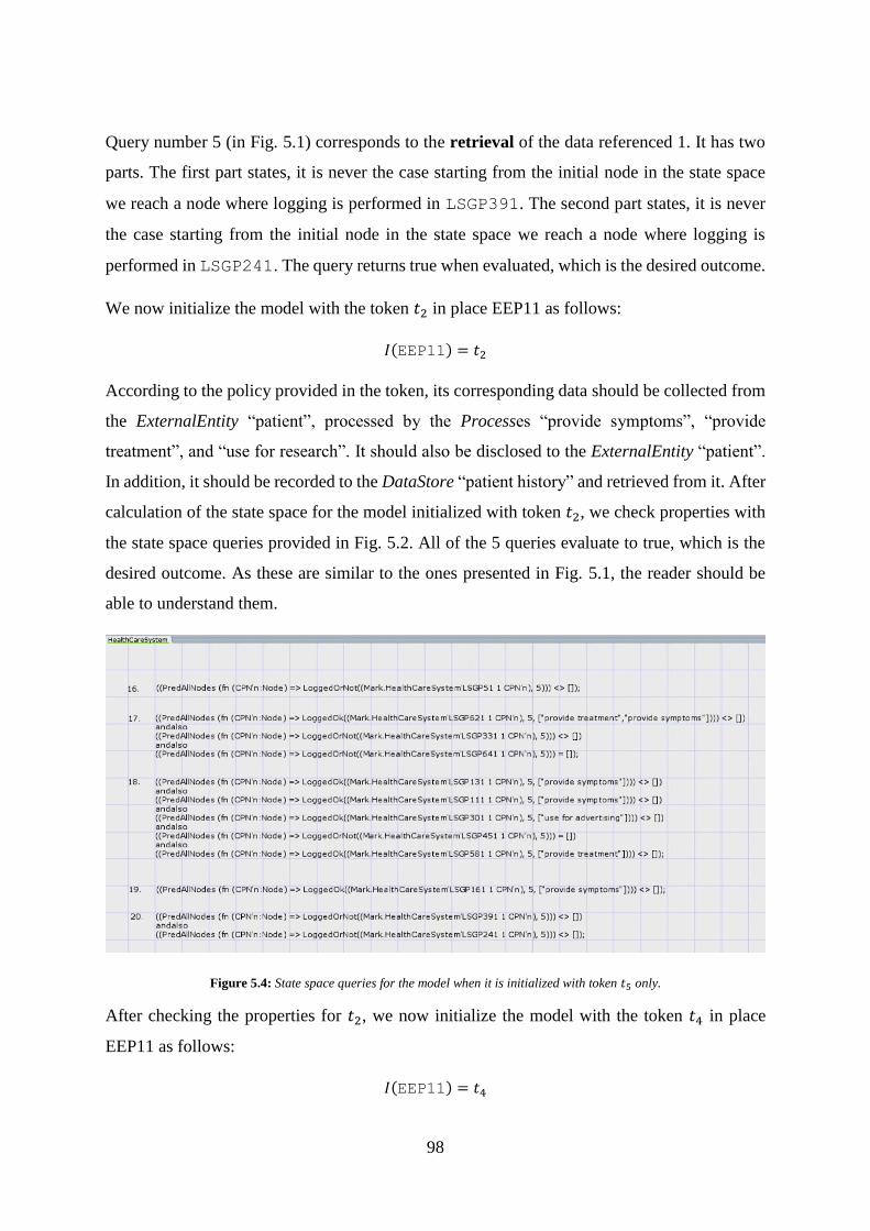
98
Query number 5 (in Fig. 5.1) corresponds to the retrieval of the data referenced 1. It has two
parts. The first part states, it is never the case starting from the initial node in the state space
we reach a node where logging is performed in LSGP391. The second part states, it is never
the case starting from the initial node in the state space we reach a node where logging is
performed in LSGP241. The query returns true when evaluated, which is the desired outcome.
We now initialize the model with the token 𝑡2 in place EEP11 as follows:
𝐼(EEP11) = 𝑡2
According to the policy provided in the token, its corresponding data should be collected from
the ExternalEntity “patient”, processed by the Processes “provide symptoms”, “provide
treatment”, and “use for research”. It should also be disclosed to the ExternalEntity “patient”.
In addition, it should be recorded to the DataStore “patient history” and retrieved from it. After
calculation of the state space for the model initialized with token 𝑡2, we check properties with
the state space queries provided in Fig. 5.2. All of the 5 queries evaluate to true, which is the
desired outcome. As these are similar to the ones presented in Fig. 5.1, the reader should be
able to understand them.
Figure 5.4: State space queries for the model when it is initialized with token 𝑡5 only.
After checking the properties for 𝑡2, we now initialize the model with the token 𝑡4 in place
EEP11 as follows:
𝐼(EEP11) = 𝑡4

99
The only thing different in 𝑡4 from 𝑡2 is the policy for the corresponding data includes the
consent of it to go through the Process “use for advertising” instead of “use for research”.
Therefore, the properties checked for 𝑡4 will be almost similar to the ones checked for 𝑡2 with
slight changes. The state space for the model with this token is calculated and properties are
checked by means of the state space queries. They are presented in Fig. 5.3. All of them return
true as expected.
Thus far, we have checked properties for the tokens 𝑡1, 𝑡2 and 𝑡4. We now initialize the model
with the token 𝑡5 in place EEP11 as follows:
𝐼(EEP11) = 𝑡5
There is a difference between token 𝑡4 and 𝑡5. The latter includes an extra consent in the policy
for the corresponding data: “health insurance company”, which allows the data to be disclosed
to the ExternalEntity of that name. After initializing 𝑡5, we calculate the state space of the
model for it. Then we check the properties for it using the state space queries and they are
presented in Fig. 5.4.
We have checked properties for all of the tokens we intend to, except 𝑡3. The consent given in
the policy for its corresponding data in 𝑡3 includes a consent “erase”. Our aim is to check
whether erasure of personal data from the DataStore happens or not. For that purpose, we need
to initialize another token in the place PrP522, which will include the reference and policy
for the data in 𝑡3. We initialize the model with the token 𝑡3 as follows:
𝐼(EEP11) = 𝑡3
Figure 5.5: State space queries for the model when it is initialized with token 𝑡3 along with another token for erasure.
We mentioned earlier in the previous chapter (when explaining the DFD for the case study),
the model is a subset of a larger model where it can be even more comprehensive and can have
much more components and flows. We assume, the place PrP522 (Process “manage”) was
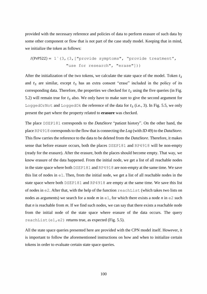
100
provided with the necessary reference and policies of data to perform erasure of such data by
some other component or flow that is not part of the case study model. Keeping that in mind,
we initialize the token as follows:
𝐼(PrP522) = 1`(3,(3,["provide symptoms", “provide treatment”,
"use for research", "erase"]))
After the initialization of the two tokens, we calculate the state space of the model. Token 𝑡2
and 𝑡3 are similar, except 𝑡3 has an extra consent “erase” included in the policy of its
corresponding data. Therefore, the properties we checked for 𝑡2 using the five queries (in Fig.
5.2) will remain true for 𝑡3 also. We only have to make sure to give the second argument for
LoggedOrNot and LoggedOk the reference of the data for 𝑡3 (i.e., 3). In Fig. 5.5, we only
present the part where the property related to erasure was checked.
The place DSEP181 corresponds to the DataStore “patient history”. On the other hand, the
place RP4918 corresponds to the flow that is connecting the Log (with ID 49) to the DataStore.
This flow carries the reference to the data to be deleted from the DataStore. Therefore, it makes
sense that before erasure occurs, both the places DSEP181 and RP4918 will be non-empty
(ready for the erasure). After the erasure, both the places should become empty. That way, we
know erasure of the data happened. From the initial node, we get a list of all reachable nodes
in the state space where both DSEP181 and RP4918 are non-empty at the same time. We save
this list of nodes in e1. Then, from the initial node, we get a list of all reachable nodes in the
state space where both DSEP181 and RP4918 are empty at the same time. We save this list
of nodes in e2. After that, with the help of the function reachList (which takes two lists on
nodes as arguments) we search for a node m in e1, for which there exists a node n in e2 such
that n is reachable from m. If we find such nodes, we can say that there exists a reachable node
from the initial node of the state space where erasure of the data occurs. The query
reachList(e1,e2) returns true, as expected (Fig. 5.5).
All the state space queries presented here are provided with the CPN model itself. However, it
is important to follow the aforementioned instructions on how and when to initialize certain
tokens in order to evaluate certain state space queries.
101
6 Discussion
The Petri nets semantics presented in this thesis captures most of the behaviors of PA-DFDs.
There are also some other behaviors that it fails to capture. PA-DFDs deal with lot more diverse
components and flows than DFDs. Therefore, an appropriate classification of those is made,
which in turn is convenient for the CPN transformation. Using CPN and its modeling language,
the core elements of PA-DFDs (data and policies) are implemented. Manipulating the
connections between transitions and places allows to model different components of PA-DFDs
and their behaviors. Apart from that, verification is performed using CPN Tools on the obtained
CPN model from a given PA-DFD model. The verification done and presented in this thesis,
are far from exhaustive. However, the resources, albeit inconsistent and somewhat outdated,
are there to be exploited further to gain comprehensive knowledge to performing verification
more elegantly.
One behavior of the PA-DFDs that the proposed Petri nets semantics is unable to capture, is
the notion of time. In PA-DFDs, it is called retention time of personal data. Retention time is
included along with the consents given in the policy of a corresponding data. When the
retention time expires for certain personal data, it is deleted from the system by means of Clean.
This can be modeled as a ticking clock or a countdown timer where it is kept in check whether
or not the time has expired for the data. If this approach was taken to model it in CPN, then the
transition representing Clean and the transitions representing the connections between Clean
and other components should have higher priority than any other transitions in the model (as
immediately the retention time expires, Clean should execute the removal of the data). Priority
wise, this is how Clean is represented in the proposed Petri nets semantics. However, there is
no notion of time used in it. Therefore, the use of Clean does not occur in this semantics. In
timed CPN and CPN Tools, the tokens are timed and there is a global clock for the model. It is
possible to add time to the token’s time via the arc expressions or when it goes through a
transition. On the other hand, the global clock neither acts as a ticking clock, nor as a
countdown timer. The time of the global clock passes the amount that is added to the token
while the token goes through a transition. Moreover, time of a token can only be increased, but
not decreased. Also, it is not possible to access time of a token directly in order to compare
with another time or the global clock’s time. For such reasons, implementing the notion of time
in PA-DFDs to CPN models becomes cumbersome.
102
Another notable behavior that the Petri nets semantics presented in this thesis is unable to
capture, is when there are more than one incoming personal data flow to a Process. When a
single incoming personal data goes through a Process, its corresponding policy is forwarded
through Reason beforehand. However, when there are more than one incoming personal data
𝑑1 (having policy 𝑝1) and 𝑑2 (having policy 𝑝2) to a Process and an outgoing data 𝑑3 from it,
it is not defined for Reason how to produce a policy for 𝑑3 from 𝑝1 and 𝑝2. One way to address
this could be to take the most restrictive policy out of the two, but it is still to be decided what
approach will suit best in this case. Taking this into account, the proposed CPN semantics of
Process is kept simple capturing the case when it is given a single personal data as input, rather
than multiple ones.
Other than the uncaptured behaviors from PA-DFDs, verification performed in the CPN model
from the case study was far from exhaustive. Due to some notable shortcomings from CPN
Tools, performing verification task was troublesome. As can be seen from section 4.3, the CPN
model obtained from the case study is extremely large. Therefore, the state space for it becomes
even larger and takes a huge amount of time to generate. The initial idea was to initialize the
place EEP11 with 10 different tokens and the place PrP522 with few more at once. However,
with that amount of tokens, the calculation of state space becomes understandably even larger.
The calculation took a lot of time and eventually did not get finished as CPN Tools randomly
crashed during the process. After several tries, the amount of tokens was lessened by half. Still,
that had no effect on the calculation. Later, it was decided to initialize the place EEP11 with
two tokens at once. Then, calculation of the state space was performed, which surprisingly
enough, did not get finished after half an hour. It is worth mentioning, a university machine
(desktop computer) was used in order to perform these tasks. The author’s personal computer
(laptop) was worse in terms of performance. In order to make sure at least some verification
can be performed, eventually it was decided to use one token at a time and calculate the state
space separately for each of them. This approach also took some time for tokens that covered
the model more. Following this approach, it was possible to check some properties by means
of state space queries and defining some CPN ML functions. It would be convenient if there
was an option to save the calculated state space. With such approach, even if the state space
takes a lot of time to generate, we only have to generate it once and load it every time we
perform verification on it. However, as there is no way to do such thing, with a limited time
103
frame for the thesis work, it is not feasible to work with such a huge state space. Moreover,
when managing models of this size, the tool tend to crash unexpectedly.
6.1 Future Work
There are a number of potential ways future research can improve the Petri nets semantics for
the PA-DFDs presented in this thesis along with the verification performed on it. We list some
significant ones below:
As mentioned earlier, the Petri nets semantics presented in the thesis does not capture
the notion of time from PA-DFDs. Therefore, a next step would be to find an effective
way to extend the semantics with time.
The CPN transformation for the component Process presented in the thesis has some
limitations. One reason for that is the definition for the component Reason is still a
work in progress. After that is resolved, a more efficient transformation is needed for
this component.
In this thesis, we perform the transformation and implement the CPN model manually
in CPN Tools. However, an automatic implementation is the ideal goal for
implementing the model. Therefore, it is a natural candidate to be a future work.
The size of a CPN model for its corresponding PA-DFD model is quite large. We cannot
help but address the redundancy of components in a PA-DFD model. If there is a way
to decrease the size of the PA-DFD model keeping the behavior as well as the
relationship between components same, then the transformation to CPN will also result
in a smaller model.
Verification of the CPN model obtained from a corresponding PA-DFD model can be
improved and done in a more comprehensive manner. As mentioned earlier, due to
some shortcomings of CPN Tools as well as the time frame of the thesis work, it was
harder to perform a comprehensive verification of the model in this thesis. Furthermore,
a good amount of knowledge regarding verification techniques in CPN Tools ([21],
[32], [33]) is also needed, which will take time considering the instructions available
are quite inconsistent. Although we have progressed with CPN Tools for
implementation as well as the verification of the model in this thesis, it is not absolutely
mandatory to use the tool. The transformation provided for the PA-DFDs can also be
implemented in some other better Petri nets tool provided that supports necessary

104
concepts used for the transformation. This area needs further exploring in future
research too.
Finally, due to the lack of formal semantics for PA-DFDs, we leave proving the
correctness of the transformation as future work.
105
7 Conclusion
New information systems are built rapidly making collection of personal data an ever
increasing factor. This raises the importance of privacy of personal data. Privacy by Design
(PbD) is an effective way to address this. Keeping that in focus along with important privacy
principles stated in GDPR, PA-DFDs are proposed to tackle privacy of personal data from the
earliest of stages of information system design. However, it is not possible to perform formal
verification on PA-DFDs because it lacks concrete semantics.
In this thesis, we explored the DFDs, PA-DFDs and different variants of Petri nets. The aim
was to give a Petri nets semantics by defining appropriate transformations for PA-DFDs,
demonstrate the effectiveness of the transformations on a case study, and to perform
verification tasks on the Petri nets model obtained from the case study.
Firstly, we use Colored Petri Nets (CPN) as the suitable Petri nets variant to give a semantics
for PA-DFDs. We do that by giving transformation algorithms (which uses formal definition
of CPN) for different PA-DFD components and flows. In order to do that, we classify various
PA-DFD components and flows beforehand. Then, we follow a modular approach for the
transformations, where for a given PA-DFD, we first transform each component to suitable
CPN representation. When we finish doing that for all the components of the model, we start
transforming the flows to their suitable CPN representations. Upon finishing these
transformations, we obtain a complete CPN model that corresponds to the PA-DFD provided
prior to the transformation.
Secondly, we conduct a case study for a subset of a health care information system design
where we apply the transformations defined earlier. We start with a DFD of the system. The
DFD was designed in such a way, so that all the privacy hotspots are included. After applying
appropriate transformations on the identified hotspots in the DFD, we get a PA-DFD. Finally,
we obtained a CPN model by means of applying the transformations defined in this thesis on
the PA-DFD. We implemented the CPN model manually in CPN Tools. The case study was
helpful in pointing out some of the missing cases in the transformation algorithms (defined in
this thesis), which led to fixing of them so that they can capture such cases.
Finally, we perform verification tasks on the obtained CPN model from the case study. CPN
Tools was used for this purpose. With the use of CPN ML and state space queries, we were
106
able to check some privacy properties such as logging, erasure and purpose limitation for the
model. The properties checked in this thesis is trivial, but with more time and comprehensive
knowledge of the verification techniques in CPN Tools, it is possible to check more interesting
privacy properties. Apart from that, other Petri nets tool can also be used for implementation
and verification purpose.
The Petri nets semantics for PA-DFDs presented in this thesis are concrete, making it possible
for verification tasks to be carried out. It is, however, beckons further research in future for
improvement with the evolution of PA-DFDs.
Above all, the Petri nets semantics presented along with the rest of the supporting work done
in this thesis establish a step forward when it comes to privacy of personal data in information
systems.
107
References
[1] A. Dennis et al., System Anal. and Design, 5th ed. John Wiley & Sons, 2012.
[2] R. Ibrahim and S. Yen, "Formalization of the Data Flow Diagram Rules for Consistency
Check", Int. J. of Software Eng. & Applicat, vol. 1, no. 4, pp. 95-111, 2010.
[3] T. Antignac et al., "A privacy-aware conceptual model for handling personal data", in
Leveraging Applicat. of Formal Methods, Verification and Validation: Foundational
Techniques, Corfu, Greece, 2016, pp. 942-957.
[4] T. Antignac et al., "A Formal Approach to Design Privacy-Aware Software Syst.".
[5] C. A. Petri, “Kommunikation mit Automaten.” Bonn: Institut fur lnstrumentelle
Mathematik, Schriften des IIM Nr. 3, 1962. Also, English translation, “Communication with
Automata.” New York: Griffiss Air Force Base.Tech. Rep. RADC- TR-65-377, vol. 1, SUPPI.
1, 1966.
[6] Handbook of Dynamic System Modeling, Taylor & Francis Group, LLC, 2007.
[7] K. Venkatesh et al., "Comparing ladder logic diagrams and Petri nets for sequence
controller design through a discrete manufacturing system," IEEE Trans. on Ind. Electronics,
vol. 41, no. 6, pp. 611-619, 1994.
[8] M. C. Zhou and F. Dicesare, "Adaptive design of Petri net controllers for error recovery in
automated manufacturing Syst.," IEEE Trans. on Syst., Man, and Cybernetics, vol. 19, no. 5,
pp. 963-973, 1989.
[9] G. Booch, et al., The Unified Modeling Language User Guide. (2nd ed.) Upper Saddle
River, NJ: Addison-Wesley, 2005.
[10] S.K. Andreadakis and A.H. Levis, “Synthesis of distributed command and control for the
outer air battle”, DTIC Document, 1988.
[11] M. Ajmone Marsan et al., Performance evaluation of multiprocessor syst.. Cambridge,
Mass.: MIT Press, 1986.
[12] W. Aalst and K. Hee, Workflow management: models, methods, and syst.. Cambridge,
Mass.: The MIT Press, 2004.
108
[13] F. Tisato et al., "Architectural Reflection Realising Software Architectures via Reflective
Activities", Eng. Distributed Objects, pp. 102-115, 2001.
[14] R. Van Landeghem and C. Bobeanu, "Formal modeling of supply chain: an incremental
approach using Petri nets", in 14th European Simulation Symp., 2002.
[15] D. Mandrioli et al., "A Petri net and logic approach to the specification and verification of
real time syst.", Formal Methods for Real-Time Computing, vol. 5, 1996.
[16] J. Tsai et al., "Timing constraint Petri nets and their application to schedulability anal. of
real-time system specifications", IEEE Trans. on Software Eng., vol. 21, no. 1, pp. 32-49, 1995.
[17] J. Wang, "Charging Inform. Collection Modeling and Anal. of GPRS Networks", IEEE
Trans. on Syst., Man and Cybernetics, Part C (Applicat. and Reviews), vol. 37, no. 4, pp. 473-
481, 2007.
[18] K. Jensen, "Coloured petri nets and the invariant-method", Theoretical Comput. Sci., vol.
14, no. 3, pp. 317-336, 1981.
[19] R. Milner, M. Tofte, R. Harper and D. MacQueen, The definition of standard ML (revised).
London: MIT Press, 1997.
[20] J. Ullman, Elements of ML programming. New Jersey: Prentice-Hall, 1998.
[21] K. Jensen and L. Kristensen, Coloured Petri Nets. Berlin, Heidelberg: Springer Berlin
Heidelberg, 2009.
[22] B. Berard et al., Syst. and Software Verification. Springer, 2001.
[23] R. Milner, Communication and concurrency. London: Prentice Hall, 1989.
[24] “The Edinburgh Concurrency Workbench,” The University of Edinburgh School of
Informatics. [Online] Available: http://homepages.inf.ed.ac.uk/perdita/cwb/index.html.
[25] D. Harel, "Statecharts: a visual formalism for complex syst.", Sci. of Comput.
Programming, vol. 8, no. 3, pp. 231-274, 1987.
[26] R. Hilliard, "Using the UML for Architectural Description", Lecture Notes in Comput.
Sci., pp. 32-48, 1999.
109
[27] G. Holzmann, Spin Model Checker, The: Primer and Reference Manual. Addison-Wesley
Professional, 2003.
[28] “Spin - Formal Verification,” Verifying Multi-threaded Software with Spin. [Online]
Available: http://spinroot.com/.
[29] R. Alur and D. Dill, "A theory of timed automata", Theoretical Comput. Sci., vol. 126, no.
2, pp. 183-235, 1994.
[30] K. Larsen, P. Pettersson and W. Yi, "Uppaal in a nutshell", Int. J. on Software Tools for
Technology Transfer, vol. 1, no. 1-2, pp. 134-152, 1997.
[31] “Design/CPN Online,” Design CPN, Jan. 17, 2006. [Online] Available:
www.daimi.au.dk/designCPN.
[32] “CPN Tools homepage,” CPN Tools. [Online] Available: www.cpntools.org.
[33] “CPN Tools State Space Manual,” CPN Tools, Jan., 2006. [Online] Available:
http://cpntools.org/_media/documentation/manual.pdf.
[34] S. Gurses and J. del Alamo, "Privacy Eng.: Shaping an Emerging Field of Research and
Practice", IEEE Security & Privacy, vol. 14, no. 2, pp. 40-46, 2016.
[35] E. Falkenberg, R. V. D. Pols, and T. V. D. Weide, “Understanding process structure
diagrams,” Inform. Syst., vol. 16, no. 4, pp. 417-428, 1991.
![Automatic Parameterisation of Stochastic Petri Net Models ...2.2 Stochastic Petri nets The theory of Petri nets [25] provides a graphical notation with a formal math-ematical semantics](https://img.pdfslide.net/doc/110x75/5f41a1a7a11fe517204266fd/automatic-parameterisation-of-stochastic-petri-net-models-22-stochastic-petri.jpg)