Embed Size (px)
Citation preview

Michigan Technological UniversityDigital Commons @ Michigan
TechDissertations, Master's Theses and Master's Reports- Open Dissertations, Master's Theses and Master's Reports
2015
A PETROPHYSICAL EVALUATION OF THETRENTON-BLACK RIVER FORMATION OFTHE MICHIGAN BASINLu YangMichigan Technological University
Copyright 2015 Lu Yang
Follow this and additional works at: http://digitalcommons.mtu.edu/etds
Part of the Geology Commons
Recommended CitationYang, Lu, "A PETROPHYSICAL EVALUATION OF THE TRENTON-BLACK RIVER FORMATION OF THE MICHIGANBASIN", Master's Thesis, Michigan Technological University, 2015.http://digitalcommons.mtu.edu/etds/914

A PETROPHYSICAL EVALUATION OF THE
TRENTON-BLACK RIVER FORMATION OF
THE MICHIGAN BASIN
By
Lu Yang
A THESIS
Submitted in partial fulfillment of the requirements for the degree of
MASTER OF SCIENCE
In Geology
MICHIGAN TECHNOLOGICAL UNIVERSITY
2015
© 2015 Lu Yang

This thesis has been approved in partial fulfillment of the requirements for the
Degree of MASTER OF SCIENCE in Geology.
Department of Geological and Mining Engineering and Sciences
Thesis Advisor: Wayne D. Pennington
Committee Member: Mir Sadri
Committee Member: James R. Wood
Department Chair: John S. Gierke

Table of Contents
Acknowledgement .......................................................................................... 4
Abstract........................................................................................................... 5
1. Introduction ............................................................................................. 6
2. Geology of Trenton-Black River Formation......................................... 6
3. Methodology ...........................................................................................10
3.1 Picking Formation Tops .......................................................................................... 10
3.2 Crossplot and Mineral Identification ...................................................................... 13
4. Thomas Stieber Method ........................................................................30
5. Discussion ...............................................................................................38
6. Conclusion ..............................................................................................39
References .....................................................................................................41
Appendix I: Crossplots & Mineral Identification ....................................42
Appendix II: Thomas Stieber (Thomas and Stieber 1975) ......................49
3

Acknowledgement
I would like to express the deepest appreciation to my advisor Dr. Wayne D. Pennington
for his expert guidance and full support. His experience and ability improved my research
skills. My thesis work would not have been possible without his help and incredible
patience.
I would like to thank my committee members, Professor James R. Wood and Professor Mir
Sadri, for helping me during my graduate years and their helpful suggestions and comments
on my research work. I am also thankful to Carol J. Asiala for helping me obtain the data
and guiding me through the Surfer software.
Thanks also go to my fellow graduate students, especially Nayyer Islam; I obtained much
benefit from working with him on the Powerlog software, and he gave me a lot of help and
advice to my research. I also have to express my appreciation to Qiang Guo and Yeliz
Egemen; with your support, I finally overcome the difficulties during the research and
finished it.
I would also like to thank my parents and friends for their support and they always
encourage me to be the best. I am very blessed to have you all in my life.
4

Abstract
This work is conducted to study the geological and petrophysical features of the Trenton-
Black River limestone formation. Log curves, crossplots and mineral identification
methods using well-log data are used to determine the components and analyze changes in
lithology. Thirty-five wells from the Michigan Basin are used to define the mineralogy of
Trenton-Black River limestone. Using the different responses of a few log curves,
especially gamma-ray, resistivity and neutron porosity, the formation tops for the Utica
shale, the Trenton limestone, the Black River limestone and the Prairie du Chien sandstone
are identified to confirm earlier authors’ work and provide a basis for my further work.
From these, an isopach map showing the thickness of Trenton-Black River formation is
created, indicating that its maximum thickness lies in the eastern basin and decreases
gradually to the west. In order to obtain more detailed lithological information about the
limestone formations at the thirty-five wells, (a) neutron-density and neutron-sonic
crossplots, (b) mineral identification methods, including the M-N plot, MID plot, maa vs.
Umaa MID plot, and the PEF plot, and (c) a modified mineral identification technique are
applied to these wells. From this, compositions of the Trenton-Black River formation can
be divided into three different rock types: pure limestone, partially dolomitized limestone,
and shaly limestone. Maps showing the fraction of dolomite and shale indicate their
geographic distribution, with dolomite present more in the western and southwestern basin,
and shale more common in the north-central basin. Mineral identification is an independent
check on the distribution found from other authors, who found similar distributions based
on core descriptions.
The Thomas Stieber method of analysis is best suited to sand-shale sequences, interpreting
three different distributions of shale within sand, including dispersed, laminated and
structural. Since this method is commonly applied in clastic rocks, my work using the
Thomas Stieber method is new, as an attempt to apply this technique, developed for
clastics, to carbonate rocks. Based on the original assumption and equations with a
corresponding change to the Trenton-Black River formation, feasibility of using the
Thomas Stieber method in carbonates is tested. A graphical display of gamma-ray versus 5

density porosity, using the properties of clean carbonate and pure shale, suggests the
presence of laminated shale in fourteen wells in this study. Combined with Wilson’s study
(2001), it is safe to conclude that when shale occurs in the Trenton-Black River formation,
it tends to be laminated shale.
1. Introduction
The Trenton-Black River formation is a Middle Ordovician carbonate present throughout
the Michigan Basin, a sedimentary and structural basin located on the Lower Peninsula.
The basin depocenter is located in near Saginaw Bay. The basin is a simple, undeformed
cratonic basin with a radius of one hundred and fifty km and about five km of depth.
(Howell and van der Pluijm 1990) Several structural elements flank the southern portion
of the Michigan Basin: Kankakee Arch, Cincinnati Arch and Findlay Arch, serving as
boundaries between the Michigan Basin and surrounding Illinois and Appalachian basins.
Many formations in the Michigan Basin are sources of petroleum. The Michigan basin
extends into Ontario, Canada, where operators are making an effort to develop the oil and
gas potential. Much of the increasing drilling activity in the Michigan basin can be
attributed to the exploration and production of the Trenton-Black River formation. In 2013,
the leader of oil exploration was in the Trenton-Black River formation in Jackson, Lenawee
and Washtenaw Counties. During mid-November of 2014, forty-six of one hundred and
twenty-five wells drilled in the state were located in the three counties (Talley 2014).
2. Geology of Trenton-Black River Formation
According to a study by Wylie et al. (2004) more than three thousand and seven hundreds
wells have been drilled in the Ordovician Trenton-Black River formations of the Michigan
basin, and most Trenton well penetrations and Trenton-Black River production wells fell
on southeastern basin. In order to obtain more detailed information of Trenton-Black River
formations, isopach and topographic maps of Trenton-Black River formation are prepared
to map the trend of the thickness and the distribution of dolomitization and shale. The
6

mineral identification is an independent check on the distribution found from Wylie et al.
(2004) and Ives (1960). Logs for thirty-five wells within the Michigan Basin are used in
this work. Figure 2.1 presents the thickness map and the depth contour map of the Trenton-
Black River formation. The background color represents the top depth of Trenton
limestone, which shows that the deepest top is at the center, but the gray contour lines
display that Trenton-Black River formation has its maximum thickness in the eastern basin
and decreases gradually to the western part. The maximum thickness is not at the center
but in the eastern basin, and is also not at the location of the deepest portion of the Trenton
formation. In eastern Michigan, the maximum thickness of the formation is about one
thousand feet. In the western and southwestern Michigan, the formation is less than four
hundred feet thick (Ives 1960).
Figure 2.1 Thickness and depth contour map of Trenton-Black River formation. The gray
contour lines display the thickness in feet with an interval of fifty ft. The background color
displays the tops of Trenton limestone with an interval of five hundred ft. 7

The Trenton-Black River formation is primarily a brown to gray crystalline limestone. Two
geologic maps are created in order to study the geographic distribution of dolomite and
shale within it. For the first map, based on the modified mineral identification (explained
in Chapter 4), the fractions of four minerals, limestone, dolomite, sandstone and shale are
calculated. Not all wells have the PEF log required for this technique, so there are twenty-
six wells used for this calculation. Figure 2.2 displays the average dolomite fraction in the
Trenton-Black River formation based on those twenty-six wells. The higher fraction of
dolomite lies in the western and southwestern portion of the basin and the lower fraction
of dolomite in the southeastern and central basin. These results are consistent with an
earlier study by Ives (1960) that found limestone and dolomite both present in the
southeastern and south central basin, but in the western and southwestern basin, the
dolomite concentration is much higher.
Figure 2.2 Contour map of Trenton-Black River formation indicating dolomite fraction by
color. 8

For the second map, shale content based on twenty-six wells are displaying with modified
mineral identification. The basal unit of Trenton-Black River formation is a very thin unit,
which contains gray to green calcareous shale, lying unconformably over older Ordovician
and Cambrian from the west to east. The entire unit of Trenton limestone is about thirty
feet, and a black dolomitic shale bed is at its base. Figure 2.3 displays the average shale
fraction in the Trenton-Black River formation. The higher shale fraction is in the north
central part of the basin, which is at the deepest point for the top of Trenton limestone
formation.
Figure 2.3 Contour map of Trenton-Black River formation showing the average fraction of
shale.
9

3. Methodology
In order to obtain the detailed lithological features of the Trenton-Black River formation
displayed in the maps shown in Figures 2.2 and 2.3, a determination of mineralogy and
porosity is made, particularly being concerned with the mineral types and their fractions.
Thirty-five wells are used in this analysis from log data available through the Michigan
Department of Environmental Quality. The compensated neutron porosity, sonic log, bulk
density, density porosity, gamma-ray log and PEF log are required for the analyses
presented in this section. The process started with picking tops of the formations from the
logs. Then, I used conventional crossplotting techniques to determine primary lithology at
the wells selected for this study. Using another technique for “modified mineral
determination,” the results shown in Figures 2.2 and 2.3 are obtained; these maps are
compared with the results obtained from the conventional techniques as well.
3.1 Picking Formation Tops
The Trenton limestone in the Michigan basin is overlain by Utica shale, which is a
traditional shale with high quartz and clay content and very little carbonate. The Utica shale
presents higher gamma-ray response than Trenton limestone due to the clay content, as
radioactive elements tend to concentrate in the impermeable shale, and are at lower
concentrations in permeable carbonates and sands. Resistivity of Utica shale is lower than
Trenton limestone because of the organic material and its higher conductivity. These traits
provide good indicators for picking the base of the Utica shale (the top of the Trenton
limestone). Additionally, Utica shale presents greater sonic transit times than Trenton
limestone; this can be attributed to the presence of clay, bound water and higher porosity
in the shale. With the presence of the bound water in clay, Utica shale has a higher neutron
porosity. These four log curves can be very useful for identifying the contact between Utica
shale and Trenton limestone.
10

In general, Trenton-Black River limestone exhibits low gamma-ray response in clean
limestone. But there are some exceptions of high amplitude spikes within it due to clay and
organic material. The resistivity response of the Trenton-Black River limestone is also
variable. Sonic transit time in Trenton-Black River limestone is lower due to the low
porosity, and some degree of dolomitization. On the other hand, the density porosity does
not provide a good indication of the boundary between Utica shale and Trenton-Black
River limestone. Since there is no hydrocarbon effect or bound water in clay, most of the
wells in Trenton-Black River limestone show lower neutron porosity response than Utica
shale (Banas 2011).
The boundary between the Utica shale and the Trenton-Black River limestone is identified
from the available log data, in order to confirm earlier authors’ work and provide a basis
for my other efforts. Two log plots of well BONINE NO 1-22 and BRAND NO 1-34 are
shown in Figure 3.1 as examples. Both of these displays include three formations: Utica
shale, Trenton limestone and Black River limestone. The green line in the first track is the
gamma-ray log; it is much higher in Utica shale than it is in Trenton-Black River formation.
The second track displays the resistivity logs, which are higher in Trenton-Black River
limestone than in Utica shale. The third track displays the porosity logs, including density
porosity, neutron porosity and average porosity (computed by averaging the other two);
Utica shale has higher porosity readings than the two limestone formations. The pink curve
in the fourth track is sonic transit time, which due to the higher porosity is greater in Utica
shale than in Trenton-Black River limestone. (Schlumberger 1991)
11

(a) (b)
12

Figure 3.1 Log plots with Utica shale, Trenton limestone and Black River limestone
formations, dotted lines are the tops of Trenton limestone and Black River limestone
formations. (a) Log plot of well BONINE NO 1-22, the depth of top of the Trenton
limestone is 2328 ft; the depth of top of the Black River limestone is 2590 ft. (b) Log plot
of well BRANDT NO 1-34.
3.2 Crossplot and Mineral Identification
Crossplots provide good tools to compare various log responses to porosity and lithology,
including shale content. In order to identify the presence of shale and recognize lithology
changes in the Trenton-Black River formation, the neutron-density and neutron-sonic
crossplots were used in this work. To further clarify the mineral mixtures, the M-N plot,
the MID plot, the maa vs. Umaa MID plot, the PEF plot and a modified mineral identification
were used.
The neutron-density crossplot with a color indicator is derived from three logs: the bulk
density, neutron porosity and gamma-ray logs. The density log contains a radioactive
source and two detectors, the radioactive source is applied to the borehole wall and emits
gamma-rays into the formation. The bulk density tool responds to the electron density of a
formation by measuring the attenuation of gamma-rays between a source and a detector.
The electron density, in turn, is related to the bulk density. The bulk density depends on
the density of the fluid, the density of the matrix, and the formation porosity. If the density
tool is calibrated in freshwater-filled formations, the apparent bulk density is related to the
electron density index. If the conditions in the borehole and formation match the calibration
conditions, the apparent bulk density is identical to actual bulk density. Neutron logs
measure the hydrogen population in a formation, and the result is related to porosity.
Specifically, the compensated neutron-porosity logging tool measures the size of a neutron
cloud from a neutron source that emits fast neutrons and two neutron detectors. Because
shale contains bound water in its structure, the neutron tool responds to the hydrogen in the
13

bound water, and reads higher neutron porosity values in the shale. Gamma-ray logging
records the natural radioactivity of a formation arising from uranium (U), thorium (Th),
and potassium (K). These three elements tend to be concentrated in shales, so the gamma-
ray log is the most common shale volume indicator. There are three lithological lines
typically overlain in the neutron-density crossplot, showing sandstone, limestone, and
dolomite lines. We generally add color to the points for gamma-ray values as a shale
indicator. From the trend of our data, we can estimate the mineral composition of the
formation under study.
The neutron-sonic crossplot with a color indicator is derived from three logs: the sonic,
neutron porosity and gamma-ray logs. The sonic logs, also known as sonic travel-time logs,
recording a sound pulse as it passes a pair of receivers, usually provided in terms of
s is influenced by physical
properties, including the formation and fluid type. The transmitter emits a sound pulse once
or twice per second, and the first arrival wave is detected by the receivers. The time elapsed
between the arrival of the first arrival wave at two receivers is the travel time. The crossplot
is similar to the neutron-density crossplot, in that lines are commonly overlain indicating
limestone, sandstone, and dolomite. Color is added from gamma-ray logs as a shale
indicator.
The M-N plot is a method of combining the three porosity logs: neutron porosity, density
porosity and sonic porosity to compute the lithology identifiers M and N. We use crossplots
of sonic-density and neutron-density to, in a sense, normalize to density and compare the
normalized values of sonic and neutron, where M is the slope of the individual lithology
lines on the sonic-density crossplot and N is the slope of the individual lithology lines on
the neutron-density crossplot; plotting data on an M-N plot provides one estimate of
lithology. The equations and property values I used are provided in Appendix I
(Schlumberger 1991).
For the MID plot, the apparent total porosity, apparent matrix transit time and apparent
grain density are required. By assuming the fluid density and using the measured bulk
14

density, we can obtain the apparent matrix density. The apparent matrix sonic velocity is
determined through the Wyllie Time-Average equation using the measured sonic velocity
and an assumed fluid velocity. A crossplot of parameters derived from these values is used
in the MID plot to provide another estimate of lithology.
The maa vs. Umaa MID plot is similar to the MID plot, this time identifying lithology with
data from the litho-density (including the photo-electric effect, or PEF) log. It uses the
apparent matrix grain density (RHOMAND) and the apparent matrix volumetric cross
section for the photo-electric effect (UMA). All the equations and parameters for the plots
are in Appendix I (Schlumberger 1991).
I applied all the crossplots and mineral identification methods to the selected 35 wells (26
wells for the techniques requiring PEF). The results can be categorized into three different
types. First, some wells display mostly pure limestone. There are five wells displaying pure
limestone. Figure 3.2 displays the names and locations of these five wells. An example of
pure limestone is shown in Figure 3.3 and Figure 3.4, which display the neutron-density
crossplot, neutron-sonic crossplot, M-N plot and PEF plot of well FERRIS AND ST
ORANGE NO 1 28. In Figure 3.3, in both the neutron-density crossplot and neutron-sonic
crossplot, the data points are almost scattered on the limestone line. Gamma-ray values of
most data points are less than 80 API. With the trend of increasing gamma-ray. There is no
significant change on the neutron porosity, density and sonic. In Figure 3.4, both the M-N
plot and PEF plot display the data points with very low gamma-ray readings, which are
less than 30 API, and obviously focus on a limestone point.
15

Figure 3.2 Names and locations of 5 wells with pure limestone.
16

Figure 3.3 FERRIS AND ST ORANGE NO 1 28 (a) Neutron-density crossplot (b)
Neutron-sonic crossplot. Data points fall on the limestone line, suggesting pure limestone
with porosities ranging up to 5% or more. Color indicates gamma-ray response, showing
mostly clean lithologies. 17

Figure 3.4 FERRIS AND ST ORANGE NO 1 28 (a) M-N plot (b) PEF plot. Data points
mainly fall on the limestone point. Color indicates gamma-ray response, showing mostly
clean lithologies. It indicates the primary mineral is limestone.
18

Another class of results show partially dolomitized limestone. There are three wells
displaying this type. Figure 3.5 displays the names and locations of the three wells. An
example of dolomitized limestone in Figure 3.6 and Figure 3.7, which displays a neutron-
density crossplot, a neutron-sonic crossplot, an M-N plot and a PEF plot of well BONINE
NO 1-22. In Figure 3.6, we see that with the increasing gamma-ray, neutron porosity also
increases, but the sonic and density log barely changes. This can be explained by secondary
porosity. Secondary porosity in carbonates is frequently caused by dolomitization. When
water carrying magnesium passes through limestone, calcite crystals will change to
dolomite, as some calcium (providing the calcite in limestone) is replaced by magnesium
(yielding dolomite). The newly formed dolomite has a smaller volume (higher density)
than the original mineral, so new porosity had to be added to the existing calcite porosity,
which is often present in the form of fractures. Dolomite has a higher matrix sonic velocity
than limestone, but due to the fractures, a higher porosity. As a matrix changes from
limestone to dolomite, the bulk density effects of increased porosity and dolomitization
may cancel each other out. Moreover, sonic logs only respond to primary porosity, ignoring
vuggy porosity and fractures, neutron log responds to the total porosity, whether large or
small, primary or secondary. So the sonic log exhibits little variation while the neutron
porosity increases. In Figure 3.7, most data points with low gamma-ray distribute between
the limestone and dolomite points, indicating varying dolomitization among the clean (non-
shaly) formations.
19

Figure 3.5 Names and locations of 3 wells with partially dolomitized limestone.
20

Figure 3.6 BONINE NO 1-22 (a) Neutron-density crossplot (b) Neutron-sonic crossplot.
With the increasing gamma-ray, neutron porosity increases, but the density and sonic log
change little. The distribution of data points can be due to the effect of the secondary
porosity. Color indicates gamma-ray responses, which are almost less than 30 API.
21

Figure 3.7 BONINE 1-22 (a) M-N plot (b) PEF plot. Data points fall on limestone and
dolomite points. Color indicates gamma-ray responses, which are less than 30 API. The
distribution of data points is affected by the secondary porosity.
22

The last type of lithology encountered in the Trenton-Black River formation is shaly
limestone. There are eighteen wells classified as exhibiting shaly limestone in this study.
Figure 3.8 displays the names and locations of the eighteen wells. An example of shaly
limestone in Figure 3.9 and Figure 3.10, which displays the neutron-density crossplot, the
neutron-sonic crossplot, the M-N plot and the MID plot of well HAROUTUNIAN UNIT
NO 1 4. In Figure 3.9, both the neutron-density crossplot and the neutron-sonic crossplot
show an increase in gamma-ray up to 60 API, and the higher gamma-ray points move
towards the clay points on these plots.
The distribution of data points in the M-N plot and the MID plot may display different
shifts depending on the lithologies involved. The direction of shifts are caused by shaliness,
secondary porosity or the presence of gas. A greater concentration of shale shifts the points
downward outside the (quartz-dolomite-calcite or sandstone-dolomite-limestone) triangle
in the M-N plot, and above or to the right of the anhydrite point in the MID plot. Secondary
porosity shifts the points up in the M-N plot, and decreases the apparent matrix transit time
in the MID plot. Gas tends to shift points upward and to the right on both the M-N plot and
the MID plot. Additional mineral constituents, other than the three primary (quartz,
dolomite, calcite) minerals considered, may cause the data points to plot outside the triangle
in the M-N or MID plots (Schlumberger 1991). In Figure 3.10, the arrow in the M-N plot
shows that data points in this well fall below the triangle in the M-N plot. The gamma-ray
values of the points in this direction are higher than those within the triangle, and one can
conclude that the shift is caused by the presence of clay minerals in shale. In the MID plot,
as the presence of shale can decrease the velocity which increases the transit time, the arrow
shows the direction of shift to the right. With increasing apparent matrix transit time and
gamma-ray, points in this direction are also above the anhydrite point. Both of the shifts in
the two plots can demonstrate the presence of shale in well HAROUTUNIAN UNIT NO
1 4.
23

Figure 3.8 Names and locations of 18 wells with shaly limestone.
24

Figure 3.9 HAROUTUNIAN UNIT NO 1 4 (a) Neutron-density crossplot (b) Neutron-
sonic crossplot. Data points fall on the limestone line. Color indicates gamma-ray
responses, which show the tendency of data points to move towards clay points.
25

Figure 3.10 HAROUTUNIAN UNIT NO 1 4 (a) M-N plot (b) MID plot. Data points
demonstrate the presence of shale.
26

In a summary of the observations made above, Figure 3.11 displays the names and
locations of all the twenty-six wells used for the crossplot evaluations. Blue points are the
five wells with pure limestone, red points are the three wells with partially dolomitized
limestone, and green points are the eighteen wells with shaly limestone. From their
distribution, we can see that most wells with shaly limestone fall on the north central part
of the basin. In general, these results compare favorably with those obtained from the
modified mineral identification technique (described in the following section) which led to
the contour maps of dolomitization in Figure 2.2 and shale fraction in Figure 2.3.
Figure 3.11 Names and locations of twenty-six wells used in crossplots. Blue points are the
five wells with pure limestone, red points are the three wells with partially dolomitized
limestone, and green points are the eighteen wells with shaly limestone.
27

With the combination of gamma-ray, the bulk density log, the PEF log and the neutron
porosity log, a modified mineral identification technique used by Islam (2011) can
determine the four mineral components and each fraction, including quartz, calcite,
dolomite and clay. Conventional three-mineral and four-mineral identification approaches
are modified by first removing the shale effect from all the logs (Islam 2011). In the 3-
mineral identification approach, gamma-ray response is often neglected, as the data
analysis is only on the basis of dry grain density (DGA) and apparent matrix volumetric
cross section (UMA) responses, sometimes limestone and clay may be replaced by
dolomite. In the 4-mineral identification approach, shale volume is changed to balance the
dry grain density (DGA) and apparent matrix volumetric cross section (UMA) responses,
so the mineral calculation would be less accurate. In order to correct the two problems, in
the modified mineral identification approach, the shale volume determined from gamma-
ray response was fixed by removing the shale effect from all the logs in the four-mineral
identification approach, including density log, porosity log and PEF log. Then apply the
corrected value with assuming linear law of volumetric mixing to the three-mineral
identification approach. (Islam 2011). All the equations, parameters and code details are
explained in Appendix I. Because some wells do not have a PEF log, this method was
applied to twenty-six wells.
I obtained a good estimate of each mineral component and displayed the results as a
lithology track in a log plot. I divided the results into three types. Most wells exhibit
limestone with a little amount of dolomite, sandstone and clay. Two wells are identified as
mostly limestone with a large amount of dolomite, and five wells show nearly pure
limestone in this formation. This approach uses DGA and UMA, which are the same
factors involved in maa vs. Umaa MID plot. Through a comparison of the lithology display
with the maa vs. Umaa MID plot, one can conclude that the modified mineral identification
approach yields results very similar to that from the crossplotting techniques. For example,
Figure 3.12(a) displays the maa vs. Umaa MID plot of well VICTORY NO 2 26, indicating
a large amount of limestone and dolomite in Trenton-Black River limestone, while 3.12(b)
displays a lithology track showing the results from the modified mineral identification
method with similar results. The results from the modified mineral identification approach
28

were summarized in Figures 2.2 and 2.3, and are similar to those obtained from the
crossplotting techniques, summarized in Figure 3.11, except three wells: Kelly 1, George
P DORR NO 1, and ENGLE NO 2-32. The three wells tend to be shaly shale and partially
dolomitized limestone, but they show less fractions on contour maps, which can be
explained by that the shale content and limestone content are less in the three wells, but
they do have the tendency to display characteristics of shaly shale and partially dolomitized
limestone.
(a) (b)
Figure 3.12 (a) maa vs. Umaa MID plot of well VICTORY NO 2 26 with Trenton-Black
River limestone, indicating the presence of limestone and dolomite; (b) Lithology display
of well VICTORY NO 2 26 with Trenton-Black River limestone, indicating the presence
of limestone, dolomite, little sandstone and clay. Green is limestone, yellow is sandstone,
purple is dolomite and grey is clay.
29

4. Thomas Stieber Method
One reason for initiating this study was to investigate the possibility of using a technique
commonly applied in clastic rocks for the study of clay distribution to the carbonates of the
Trenton-Black River formation, which is a new attempt. The Thomas Stieber method is
frequently used to distinguish shale types in sandstone using the density and gamma-ray
logs to differentiate three ways that shale can be distributed in sand: dispersed, laminated
and structural. Figure 4.1 graphically depicts these types. Dispersed shale accumulates to
the grains of the sandstone, and can decrease effective porosity, permeability and fluid
mobility, but because of the water content of clays it can increase measured water
saturation. Almost all sandstones contain some dispersed shale. Laminated shale exists as
fine layers in the rock; because the effective porosity and permeability of shale are zero,
laminated shale can decrease the overall porosity and permeability, but has no influence on
these properties within each individual thin sand bed. Structural shale takes the place of
sand grains, and can be considered as part of the rock framework; it has no effect on
porosity and permeability, but it does not occur frequently.
Figure 4.1 Clean sand and three shale types in sandstone. Yellow parts are sand grains,
grey parts are shale. (a) Clean sand; (b) Dispersed shale in sand, accumulates to the grains; 30

(c) Laminated shale in sand, existing as layers; (d) Structural shale in sand replaces the
sand grains.
Before introducing this method, an explanation of the assumptions is necessary. (1) We
assume that shale is the only factor that destroys porosity. (2) We consider the two end-
members of shaly sand to be clean sand and pure shale. (3) Because the gamma-ray log
response is sensitive to mass of radioactive grains, this method works best when the shale
and sand have similar grain density.
When dispersed shale is in the pore space, I imagine that one end-member is clean sand
and that dispersed shale is added into the pore space incrementally. The amount of
dispersed shale that can be added is limited due to the pore volume (because dispersed
shale does not displace sand), so the maximum volume of dispersed shale is the original
porosity of clean sand. After all the pore space is filled with shale, the resulting porosity is
at a minimum. For laminated shale, two end-members are clean sand and pure shale
because laminated shale both occupies pore space and replaces sand grains. The porosity
and gamma-ray values both vary linearly between the two end-members. On the other
hand, structural shale only replaces sand grains. As the porosity of solid sand grains is zero,
replacing it with shale can increase both gamma-ray values and porosity. It is useful to
normalize all the gamma-ray responses by finding gamma-ray values of clean sand and
pure shale.
Figure 4.2 shows an example of a Thomas Stieber template for sandstone with one data
point. That data point represents a shaly sand with normalized gamma-ray log value of 0.38
and density porosity of 0.22. To normalize the values, I used gamma-ray values for clean
sand and pure shale of 15 API and 100 API and density porosities of clean sand and pure
shale of 0.3 and 0.1. Equations and parameters for each type of shale are in Appendix II.
The lines in Figure 4.2, are drawn such that a triangle is formed by the three lines of
dispersed shale, laminated shale and dispersed-to-structural shale. I also created some
additional dispersed-shale lines by increasing the content of laminated shale by 10% for
each line. The location of a data point in this plot can distinguish the associated shale type
31
and its fraction. Take an example of the small yellow triangle in Figure 4.2. The normalized
gamma-ray value is 0.4 and the density porosity is 0.21, and the laminated shale content is
38%.
Figure 4.2 Thomas Stieber plot of sandstone where porosities of clean sand and shale are
0.3 and 0.1, and normalized gamma-ray of clean sand and shale are 0 and 1 respectively.
Blue line represents dispersed shale, red line represents laminated shale, green line
represents structural shale and purple line represents dispersed shale changes to structural
shale. The yellow triangle is identified with normalized gamma-ray at 0.4, density porosity
at 0.21, and laminated shale content at 38%.
The location of the triangle corners in the Thomas Stieber method are dependent on the
gamma-ray and density responses of the sand and shale. In order to apply the method to
carbonates in the Trenton-Black River limestone, I assume that the two end-members are
clean carbonate and pure shale, and obtained the appropriate values from the logs. For
example, Figure 4.3 shows a log plot of well USA ST NORMAN NO 1-29 for the Utica
shale and Trenton limestone, from which we can obtain end-member properties. The clean
carbonate exhibits porosity of 0.07 at depth 6465 feet where the gamma-ray response is 15
API. For the pure shale, I used the density porosity in Utica shale of 0.09, obtained at depth
32

6238 feet where the gamma-ray response is 150 API. These depths are indicated on the log
plot in Figure 4.3, where the gamma-ray values are the minimum and maximum.
33

Figure 4.3 Log plot of well USA ST NORMAN NO 1-29 with Utica Shale and Trenton
limestone. The green line in the first track is the gamma-ray curve, the green line in the
fourth track is the DPHI curve, dotted lines are at depths of clean carbonate and pure shale,
and the circled depths provide the gamma-ray readings and lithology for clean carbonate
(lower point) and pure shale (shallower point).
These values provide the end points for the upper side of the triangle (the laminated shale
line) in the Thomas Stieber method. To determine the lower corner of the triangle, I add
dispersed shale into the pore space of clean carbonate until the maximum amount of
dispersed shale equals the original porosity of clean carbonate.
Following the method used to read values and apply the equations of the Thomas Stieber
method, detailed in Appendix II, I obtained the density porosity of clean carbonate and
pure shale and the minimum porosity of each well independently. Then I created my own
Thomas Stieber plots for these carbonates. Figure 4.4 displays an example for well USA
ST NORMAN NO 1-29. The colored data points in this figure follow a trend along the
laminated shale line. There are fourteen wells displaying this kind of distribution in our
sample. Table 4.1 summarizes the results of Thomas Stieber and those of the crossplot
method for lithology determination.
34

Figure 4.4 Thomas Stieber plot of well USA ST NORMAN NO 1-29 with Trenton-Black
River limestone, between normalized gamma-ray and density porosity. The color bar
shows the shale volume (which also correlates with location on the horizontal axis). Black
lines represent dispersed shale, laminated shale and dispersed to structural shale. Data
points fall on the laminated shale line.
Table 4.1 List of 26 wells and results of crossplots and Thomas Stieber
Well Name Pure Limestone Partially
Dolomitized
Limestone
Shaly
Limestone
Laminated
Shale
ARMSTRONG NO 1-8
FERRIS AND ST ORANGE NO 1 28
JONES UNIT B NO 3-7
Kennedy 1-15
USA ST NORMAN NO 1-29
BONINE NO 1-22
ENGLE NO 2-32
REYNOLDS NO 2-11
BRANDT NO 1-34
BALLENTINE UNIT NO 1 35
35

COATES NO 1 24
CONSUMERS POWER CO NO 1 34
DOORNBOS NO 5-30
GERNAAT ET AL NO 2 19
GEORGE P DORR NO 1
HAROUTUNIAN UNIT NO 14
HUBER NO 1 26
Kelly 1
MARTIN NO 1-15
MAIDENS ET AL NO 5 25
N MICH LAND AND OIL 1-27
PREVOST ET AL NO 1-11
SNOWPLOW NO 9
VICTORY NO 2 26
CAMERON NO 1 10
ST MICHELL NO 1-31
As we can see from the table, most wells with shaly limestone are displayed in laminated
shale, and it may be safe to conclude that when shale occurs in the Trenton-Black River
limestone formation, it tends to be laminated. Wilson’s (2001) study described core from
Hunt Winterfield Deep A-1, and identified these facies in the Trenton-Black River
formations: hardgrounds, laminated shale beds, compacted shale seams, and cross-
laminated bioclastic units. This also suggests that the shale is laminated when it occurs.
In order to obtain more details about the laminated shale beds in Trenton-Black River
formations, I analyzed the logs from one well included in Wilson’s (2001) study: Hunt
Winterfield Deep A-1, Figure 4.5 shows the neutron-sonic crossplot; gamma-ray values,
neutron porosity and sonic transit time all increase in the direction of the arrow. The
gamma-ray increase alone demonstrates the presence of shale, while the change in other
properties can be explained by some sort of systematic variation in lithology, but which
cannot be identified by this plot alone.
36

Figure 4.5 Neutron-sonic crossplot of well Winterfield Deep Unit NO A1 in Trenton-Black
River limestone. Both neutron porosity and sonic transit time increased in the arrow’s
direction, which the gamma-ray values indicate as increasing in shale content.
The Thomas Stieber plot for well Winterfield Deep Unit NO A1 was created, picking the
Trenton-Black River formations. In Figure 4.6, the density porosities of clean carbonate
and pure shale are 0.61 and 0.66, and the minimum density porosity (which is the product
of these values) is 0.40. The normalized gamma-ray value for the minimum porosity point
can be calculated from the equation in Appendix II as 0.74 API. In the direction of the
arrow, with increasing shale volume, the content of laminated shale increases. This
distribution of the data points can be used to support Wilson’s (2001) summary.
37

Figure 4.6 Thomas Stieber plot of well Winterfield Deep Unit NO A1 in Trenton-Black
River limestone. The colored data points distribute in the arrow’s direction on the
laminated shale line, indicating the content of laminated shale increases.
5. Discussion
This work applied petrophysical analysis to the Trenton-Black River limestone formation.
The methods used consisted of conventional crossplot techniques for mineral
identification, a modified mineral identification approach, and an extension of the Thomas
Stieber method for shale distribution.
Neutron-density and neutron-sonic crossplots can indicate lithology changes and the
presence of shale in formation. But there are some limitations in the well log data. The log
curves were measured and run by different companies, so there are different charts used to
determine some parameters, which would affect the accuracy of results.
38
Compared to three-mineral and four-mineral identification, the modified mineral
identification gives reasonable good results by removing the effect of shale. The correction
makes the results more reliable. But the data quality of some wells is poor, which may
cause some uncertainties and errors. There are thirty-five wells used in this work, but nine
of these wells do not have a PEF log, and mineral components cannot be calculated without
the PEF log. Less data would also cause less accurate results of mineral identification.
In order to have more detailed information about the constituent components of carbonate,
the Thomas Stieber method was applied to the Trenton-Black River limestone formation.
The Thomas Stieber method is a combination of a gamma-ray log and a density porosity
log, distinguishing the types of shale. From the distribution of data points on the Thomas
Stieber plot, it is easy to see the presence of laminated shale in this formation.
6. Conclusion
The Trenton-Black River limestone formation is composed primarily of calcite, dolomite,
clay and small amounts of quartz. The greatest depth to the top of this formation is found
in the central basin, which has a higher shale fraction. But the maximum thickness is in the
eastern basin, not at the center, and it decreases gradually to the western part. In the
southeastern and the south central basin, limestone and dolomite are both present, but in
the west and southwest of the basin, the dolomite increases.
In order to obtain the description of the mineral composition and explain the lithology
changes, neutron-density and neutron-sonic crossplots are applied to Trenton-Black River
limestone. Each of the two crossplots gave three quite different results: pure limestone,
partially dolomitized limestone and shaly limestone.
Mineral identification is necessary for detailed lithology interpretation. The M-N plot, MID
plot, maa vs. Umaa MID plot, PEF plot and the modified mineral identification method are
involved in this work. The modified mineral identification of Islam (2011) showed results
39
similar to those of the crossplot techniques, demonstrating the presence of dolomite and
shale in the Trenton-Black River limestone formation.
The Thomas Stieber method is a model for the porosity of sand-shale sequences, which can
be used to parse shaly sand into three different types of shale: dispersed, laminated and
structural. This method is commonly used for clastic rocks, in order to apply its application
in carbonates, the Thomas Stieber approach was applied to the Trenton-Black River
limestone formation. Under the similar assumption that the rocks have two end-members
of clean carbonate and pure shale, my own plot for carbonates was created, displaying the
presence of laminated shale. Combined with Wilson’s (2001) study, his descriptions of
core from the Trenton-Black River formation can support the result from the Thomas
Steiber plot. There is a conclusion that where there is shale in the Trenton-Black River
limestone formation, it tends to be laminated shale.
40

References
Banas, R. M. 2011. Geophysical and geological analysis of the Collingwood Member of the Trenton Formation. In Geological/Mining Engineering & Sciences. Thesis (M.S.) - Michigan Technological University.
Catacosinos, P., P. Daniels Jr & W. Harrison III (1991) Structure, stratigraphy, and petroleum geology of the Michigan Basin. Interior cratonic basins: AAPG Memoir, 51, 561-601.
Coburn, T. C., P. A. Freeman & E. D. Attanasi (2012) Empirical methods for detecting regional trends and other spatial expressions in Antrim Shale gas productivity, with implications for improving resource projections using local nonparametric estimation techniques. Natural resources research, 21, 1-21.
Fara, D. & B. Keith (1984) Depositional Facies and Diagenetic History of Trenton Limestone in Northern Indiana: ABSTRACT. AAPG Bulletin, 68, 1919-1919.
Howell, P. D. & B. A. van der Pluijm (1990) Early history of the Michigan basin: Subsidence and Appalachian tectonics. Geology, 18, 1195-1198.
Islam, N. 2011. Sonic log prediction in carbonates. In Geological/Mining Engineering & Sciences. Thesis (M.S.) - Michigan Technological University.
Ives, R. E. 1960. Trenton-Black River Formation Developments in Michigan. Vol. 2 No.1 pp. 79-86. The Interstate Oil Compact Commission Committee Bulletin.
Minear, J. W. 1982. Clay models and acoustic velocities. In SPE Annual Technical Conference and Exhibition. Society of Petroleum Engineers.
Rancourt, C. 2009. " Collingwood" Strata in South-central Ontario-A Petrophysical Chemostratigraphic Approach to Comparison and Correlation Using Geophysical Borehole Logs.
Rupp, J. 1997. Tectonic features of Indiana. In Indiana Geological Survey, Tectonic Features. Indiana Geological Survey.
Schlumberger. 1991. Log interpretation principles/applications. Schlumberger Educational Services.
Talley, C. J. 2014. Oil & GAS NEWSLETTER. In Michigan State University Extension Farm Management.
41

Thomas, E. & S. Stieber. 1975. The distribution of shale in sandstones and its effect upon porosity. In SPWLA 16th Annual Logging Symposium, 4-7. Society of Petrophysicists and Well-Log Analysts.
Wylie, A. S., Jr, J. R. Wood & W. B. Harrison, III (2004) Michigan Trenton-Black River opportunities identified with sample attribute mapping. Oil & Gas Journal, 2004, ProQuest pg. 29.
Appendix I: Crossplots & Mineral Identification
There are many ways to identify minerals from logs. The methods that are addressed in
the text are summarized here, using conventional approaches found in standard logging
charts and algorithms.
1. Density Porosity and Sonic Porosity
Density porosity is related to matrix density, bulk density, and fluid density. Sonic density
is determined with Wyllie Time-Average equation.
DPHI =
DHPI = Density porosity
RhoM = Matrix
b = Bulk density (logging curve RHOB)
f
SPHI =
SPHI = Sonic density
DT = Reading on the sonic log (logging curve DT)
42

DTMA = Matrix transit time (I used 55
DTF = Fluid transit time (I
2. M-N Plot
The M-N plot is used to identify minerals based on the porosity indicators from sonic and
neutron logs, normalized by the density log.
M = 0.01
N =
tf
t = Interval transit time (logging curve DT)
b = Bulk density (logging curve RHOB)
f
Nf = Fluid neutron porosity (I used 1)
N = Neutron porosity (logging curve NPHI)
Sandstone: M = 0.835 N = 0.667
Limestone: M = 0.854 N = 0.621
Dolominte: M = 0.8 N = 0.528
3. MID Plot
The apparent total porosity, apparent matrix transit time and apparent grain density are
required for this plot. 43

maa =
maa = Apparent grain density
ta = Apparent total porosity (logging curve PHIND)
tmaa =
tmaa = Apparent matrix transit time
4. maa vs. Umaa MID
The maa vs. Umaa MID plot is similar with MID plot, identifying lithology with data from
litho-density log. It uses the apparent matrix grain density (RHOMAND) and the apparent
matrix volumetric cross section (UMA).
UMA =
e = ..
UMA = Apparent matrix volumetric cross section
Pe = Photoelectric absorption cross section (logging curve PEF)
e = Electron density
Uf
5. Modified Mineral Identification(Islam 2011)
This identification is modified by combining both 3-mineral and 4-mineral identification
approach and removing the shale effect from all the logs.
44
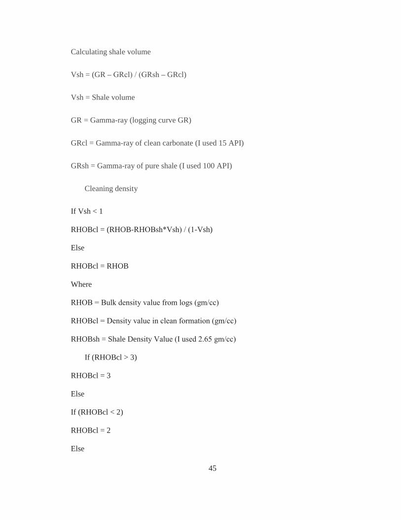
Calculating shale volume
Vsh = (GR – – GRcl)
Vsh = Shale volume
GR = Gamma-ray (logging curve GR)
GRcl = Gamma-ray of clean carbonate (I used 15 API)
GRsh = Gamma-ray of pure shale (I used 100 API)
Cleaning density
If Vsh < 1
RHOBcl = (RHOB- -Vsh)
Else
RHOBcl = RHOB
Where
RHOBsh = Shale Den
If (RHOBcl > 3)
RHOBcl = 3
Else
If (RHOBcl < 2)
RHOBcl = 2
Else
45

RHOBcl = RHOBcl
Cleaning PEF
If Vsh < 1
PEFcl = (PEF- -Vsh)
Else
PEFcl = PEF
Where
PEF = Photoelectric absorption cross section log
Cleaning neutron porosity
If Vsh < 1
NPHIcl = (NPHI-NPHIsh*Vsh)
Else
NPHIcl = NPHI
Where
NPHIcl = Neutron porosity in clean formation
NPHI = Neutron porosity from logging data
NPHIsh = Neutron porosity in shale (I used 0.25)
Cleaning density porosity
PHIDcl = (RhoM - - RhoF)
PHIDcl= Density porosity in clean formation
46
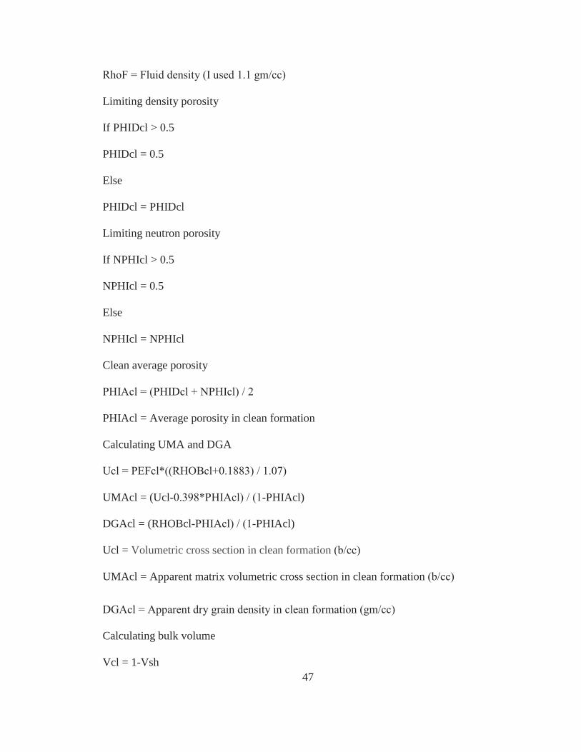
Limiting density porosity
If PHIDcl > 0.5
PHIDcl = 0.5
Else
PHIDcl = PHIDcl
Limiting neutron porosity
If NPHIcl > 0.5
NPHIcl = 0.5
Else
NPHIcl = NPHIcl
Clean average porosity
PHIAcl = Average porosity in clean formation
Calculating UMA and DGA
UMAcl = (Ucl- -PHIAcl)
DGAcl = (RHOBcl- -PHIAcl)
Ucl = Volumetric cross section in clean formation
UMAcl = Apparent matrix volumetric cross section in clean formation
Calculating bulk volume
Vcl = 1-Vsh 47

Vcl = Bulk volume in clean formation
Calculating mineral fractions(Wylie, Wood and Harrison 2004)
P1cl = (-D2*UMAcl+D3*UMAcl+DGAcl*U2-Vcl*D3*U2- -D2*U1+D3*U1+D1*U2-D3*U2-D1*U3+D2*U3)
If P1cl <0
P1cl=0
If P1cl >1
P1cl = 1
P2cl = (-D1*UMAcl+D3*UMAcl+DGAcl*U1-Vcl*D3*U1- -D2*U1+D3*U1+D1*U2-D3*U2-D1*U3+D2*U3)
If P2cl <0
P2cl = 0
If P2cl >1
P2cl = 1
P3cl = (-D1*UMAcl+D2*UMAcl+DGAcl*U1-Vcl*D2*U1- -D2*U1+D3*U1+D1*U2-D3*U2-D1*U3+D2*U3)
If P3cl <0
P3cl = 0
If P3cl >1
P3cl = 1
S = (P1cl+P2cl+P3cl)
P3cl =
48

P4cl = Vsh
U1= Limestone’s volumetric cross section
U2 = Sandstone’s volumetric cross section
U3 = Dolomite’s volumetric cross section
U4 = Clay’s volumetric cross section (I used 10
Display the calculations in the logplot
P1DSP = P1cl
P2DSP = P1cl+P2cl
P3DSP = P1cl+P2cl+P3cl
P4DSP = P1cl+P2cl+P3cl+P4cl
Appendix II: Thomas Stieber (Thomas and Stieber 1975)
Thomas Stieber method uses a combination of density log and gamma-ray log. Equations
and parameters to calculate gamma-ray, shale volume, and porosity for dispersed shale,
laminated shale and structural shale are introduced in this part.
1. Dispersed Shale
Dispersed shale accumulates to the grains of the sandstone, which can decrease effective
porosity, permeability and fluid mobility.
49

d sd + Xsh sh
d = Radioactive count rate of dispersed shale (API units)
sd = Radioactive count rate of clean sand (I used 100 API)
Xsh = Shale volume fraction
sh = Radioactive count rate of shale (I used 15 API)
When Xsh d sd d(min) sd.
When Xsh(max) = sd, d(max) sd + sd sh, d(min) sd sh
sd = Original porosity of clean sand
sh = Shale porosity
2. Laminated Shale
Laminated shale exists as layers in the rock. Since the effective porosity and permeability
of shale are zero, this type of shale can decrease the overall porosity and permeability, but
it has no influence on each individual sand bed.
l sd -Xsh sd + sh
l = Radioactive count rate of laminar shale
l = sd – Xsh sd + Xsh sh
l = Porosity of laminar shale
sh = Porosity of shale
3. Structural Shale
50

Structural shale takes the place of sand grains, it can be considered as part of the rock. It
has no effect on porosity and permeability, but it does not occur frequently.
s sd – Xsh sd + Xsd sh
s = Radioactive count rate of structural shale
s = sd + Xsh sh s = Porosity of structural shale
4. Normalized Gamma-ray
Normalized GR =
51