A PETROV-GALERKIN SPECTRAL METHOD OF LINEAR … · A PETROV-GALERKIN SPECTRAL METHOD OF LINEAR COMPLEXITY FOR FRACTIONAL MULTI-TERM ODES ... The Rodrigues formula for these ... solutions

A PETROV-GALERKIN SPECTRAL METHOD OF LINEARCOMPLEXITY FOR FRACTIONAL MULTI-TERM ODES ON THE

HALF LINE⇤

ANNA LISCHKE† , MOHSEN ZAYERNOURI‡ , AND GEORGE EM KARNIADAKIS§

Abstract. We present a new tunably-accurate Laguerre Petrov-Galerkin spectral method forsolving linear multi-term fractional initial value problems with derivative orders at most one andconstant coe�cients on the half line. Our method results in a matrix equation of special structurewhich can be solved in O(N logN) operations. We also take advantage of recurrence relations forthe generalized associated Laguerre functions (GALFs) in order to derive explicit expressions forthe entries of the sti↵ness and mass matrices, which can be factored into the product of a diagonalmatrix and a lower-triangular Toeplitz matrix. The resulting spectral method is e�cient for solvingmulti-term fractional di↵erential equations with arbitrarily many terms, which we demonstrate bysolving a fifty-term example. We apply this method to a distributed order di↵erential equation,which is approximated by linear multi-term equations through the Gauss-Legendre quadrature rule.We provide numerical examples demonstrating the spectral convergence and linear complexity of themethod.

Key words. spectral accuracy, linear complexity, singular solutions, tunable accuracy, dis-tributed order

AMS subject classifications. 34L10, 58C40, 34K28, 65M70, 65M60

1. Introduction. While numerical methods for fractional di↵erential equationshave been investigated for over two decades [1, 2, 3, 4], the main di�culty in developingthese methods, unlike their integer-order counterparts, is the large computational costdue to the non-local nature of fractional di↵erential operators. For example, in finitedi↵erence [3, 5, 6, 7] or finite element methods [8, 9], data at all grid points or elementsare needed in order to achieve an accurate approximation to the fractional derivativeat a single grid point or element. This results in methods that are significantly morecomplex in both implementation and computational cost than methods for integer-order counterparts.

Recently, spectral methods have been applied to these problems, o↵ering thebenefit of more natural non-local approximations in addition to high accuracy in thecase of smooth solutions. For non-smooth solutions with singularity of type (x� a)↵

(where a is the left endpoint of the approximation interval), we find that using anapproximation of the form (x � a)↵p(x), with p(x) a polynomial approximation tothe smooth part of the solution, will also lead to numerical approximations with ahigh order of accuracy. Zayernouri and Karniadakis derived functions of this typeas eigenfunctions of fractional Sturm-Liouville problems on a compact interval [10,11, 12, 13, 14, 15]. Khosravian-Arab et al. extended this work to fractional Sturm-Liouville problems on the half line and derived the generalized associated Laguerre

⇤Submitted to the editors February 1, 2017.Funding: This work was supported by the OSD/ARO/MURI on “Fractional PDEs for Conser-

vation Laws and Beyond: Theory, Numerics and Applications (W911NF-15-1-0562)”†Division of Applied Mathematics, Brown University, Providence, RI 02912, USA

( anna [email protected]).‡Department of Computational Mathematics, Science, and Engineering, Michigan State Univer-

sity, 428 S. Shaw Lane, East Lansing, MI 48824, USA and Department of Mechanical Engineering,Michigan State University, 428 S. Shaw Lane, East Lansing, MI 48824, USA ([email protected]).

§Corresponding author. Division of Applied Mathematics, Brown University, Providence, RI02912, USA(george [email protected]).

1

mailto:[email protected]

2 ANNA LISCHKE, MOHSEN ZAYERNOURI, AND GEORGE EM KARNIADAKIS

functions (GALFs) [16].Laguerre polynomials have been used for decades as basis functions in spectral

methods for solving integer-order di↵erential equations on the half line [17]. Thesepolynomials are solutions of Laguerre’s equation:

xy

00 + (↵+ 1� x)y0 + ny = 0,(1)

where ↵ 2 R is the parameter for the associated Laguerre polynomials, and y =

L

(↵)n (t). The Rodrigues formula for these polynomials is

L

(↵)n (t) =

t

�↵e

t

n!

d

n

dx

n(e�t

t

n+↵),(2)

and they satisfy the recurrence relation

L

(↵)n (x) =

nX

i=0

✓

↵� � + n� i� 1

n� i

◆

L

(�)i (x),(3)

where � is another associated parameter in R. These polynomials are particularlyuseful in the context of solving equations defined in semi-infinite domains becausethey satisfy an orthogonality relation on the half line:

Z 1

0

L

(↵)n (t)L(↵)

k (t)e�tt

↵dt =

�(n+ ↵+ 1)

�(n+ 1)�nk.(4)

The two types of GALFs used in our work are discussed in Section 2.2 and are definedas

�

↵,1n (t) := t

↵L

(↵)n (t), n = 0, 1, 2, . . . , ↵ > 0,(5)

�

↵,2n (t) := e

�tL

(↵)n (t), n = 0, 1, 2, . . . , ↵ > �1.(6)

These functions were shown to be solutions of fractional Sturm-Liouville problems onthe half line in [16] and are utilized here as basis functions for our Laguerre Petrov-Galerkin method for multi-term fractional initial value problems.

Zhang et al. [18] analyzed spectral methods on the half line for a single-termfractional initial value problem using a generalized version of the GALFs. The authorsof [18] derived both collocation and Petrov-Galerkin methods on bounded intervalsand on the half line, including a Laguerre PG method for single-term fractional ODEs.

Our present work di↵ers from the work by Zhang et al. in the following aspects.• We apply our Laguerre PG method to multi-term equations, which increasesthe complexity of the problem significantly because the sti↵ness matrix be-comes dense and therefore computationally di�cult to assemble and invert.In the single-term case studied in [18], all sti↵ness matrices are diagonal.

• We provide explicit expressions for the sti↵ness matrix entries in the multi-term case, thus avoiding the computational cost of applying quadrature rulesto integrals of singular functions and assembling the sti↵ness and mass ma-trices exactly.

• In our work, we develop a method of factoring the linear system into a productof diagonal and Toeplitz matrices in order to invert the system with linear

complexity. This is done by taking advantage of special recurrence propertiesof the Laguerre basis functions.

PG METHOD FOR MULTI-TERM FRACTIONAL EQUATIONS 3

• The e�ciency of our method is robust for multi-term equations that includea reaction term, which corresponds with a mass matrix in the discretizedsystem. Although mass and sti↵ness matrices typically do not have similarstructures in Petrov-Galerkin spectral methods, our method results in massmatrices which a↵ord the same type of factorization as the sti↵ness matrices.Thus when our method is applied to multi-term equations with reaction terms,the resulting matrix equation can still be solved with linear complexity.

• Further, we have applied our e�cient method to distributed order equations,which were not considered in [18].

Equations similar to those considered in our work have been considered by Baleanu,Bhrawy, and Taha in [19] and by Bhrawy, Baleanu, and Assas in [20], in which theyapply spectral Tau and collocation methods based on Laguerre polynomials to solvemulti-term fractional initial value problems on the half line. In [19] and [20], the au-thors use Newton’s iterative method and an LU decomposition respectively to solvethe resulting discrete system of equations. Both methods require O(N3) operations,where N represents the size of the system of equations. Additionally, the discretesystem resulting from these methods is dense and ill-conditioned. In comparison, ourmethod results in a well-conditioned system, which can be solved with O(N logN) op-erations. This improved e�ciency o↵ers the capability of solving multi-term equationswith many terms at low computational cost, resulting in a computationally feasibleapproximation method for the solution of distributed order equations, as detailedbelow.

There has recently been significant work on multi-term time-fractional di↵erentialequations in bounded domains [21, 22, 23, 24]. In [21], Zheng et al. use a Galerkinspace-time spectral method for a multi-term time-fractional di↵usion equation ona bounded domain. They consider equations with both two- and three-term time-fractional derivatives in one spatial dimension, and Legendre polynomials are usedas the basis functions for their space-time Galerkin method. The resulting temporalsti↵ness matrix is dense and sti↵, requiring O(N3) operations to solve. To the best ofour knowledge, all existing spectral methods for multi-term time-fractional di↵erentialequations require O(N3) operations to compute the numerical solution.

In [22], Zhao et al. consider a two-dimensional multi-term time-fractional di↵usionequation in a bounded, convex, polygonal domain, where the spatial derivative is thestandard integer-order Laplacian. They applied a finite element method in space and aclassical L1 approximation in time, achieving a convergence rate of orderO(h2+⌧

2�↵),where ↵ corresponds to the largest order of the time derivatives. The errors forthis method are evaluated at times less than t = 1, hence the problem of long-timeintegration is still of interest.

In [23], Liu et al. derive numerical methods for multi-term time-fractional wave-di↵usion equations in bounded domains using finite di↵erence methods. Two implicitfinite di↵erence schemes and two predictor-corrector Adams-Bashforth-Moulton meth-ods for the two-term time-fractional wave-di↵usion equation in one dimension areproposed. The authors use a central di↵erence scheme for the second-order spatialderivative and thus achieve second order convergence in space and 1 +min(↵i) orderconvergence in time (where {↵i} are the orders of the time-fractional derivatives).Our present work o↵ers the advantage of high-order, e�cient approximations in thecase where the solutions are smooth.

There has also been recent work on deriving analytical solutions of multi-termtime-fractional di↵erential equations [24, 25]. In [25], Ming et al. consider analyticalsolutions for unsteady flows of non-Newtonian fluids on a moving, infinite plate. The


authors expanded the solution in space using a sine series and found the solutionsof the resulting system of time-fractional ordinary di↵erential equations as a finitesum of multivariate Mittag-Le✏er functions. In [24], a similar technique was used toderive solutions for equations defined in two- and three-dimensional bounded domains.In this case, the authors consider a multi-term time- and space-fractional equations,where the two terms with di↵erent orders of the space-fractional Laplacian appear.

The multi-term equations considered in this work are motivated by the approx-imation of distributed order di↵erential equations using a quadrature rule as in thepaper by Diethelm and Ford [26]. This type of equation arises in many physical andbiological applications: for example, in applications to viscoelastic oscillators [27],distributed order membranes in the ear [28], dielectric induction [29], and anomalousdi↵usion [30, 31]. In their paper, Diethelm and Ford considered distributed orderequations of the form

Z m

0

a(r)0

Drtu(t) dr = f(t),(7)

to which they applied the trapezoid quadrature rule to derive a multi-term fractionaldi↵erential equation on a bounded interval. To improve the quality of the approxima-tion, many terms in the resulting multi-term equation may be needed. The e�ciencyand high order of accuracy of our proposed method o↵ers the capability of accuratelysolving equations with many terms with low computational cost.

The multi-term FIVPs considered in this work have fractional order at most one.There is reason to consider this problem important, as it is possible to reduce anylinear multi-term fractional equation to a system of multi-term fractional equationswith order at most one [4].

In the Petrov-Galerkin method presented in the following sections, we also intro-duce a tuning parameter enabling us to “speed up” the rate of convergence of themethod when the order of the singularity is known. In cases where the optimal valueof the tuning parameter is not known a priori, our numerical results demonstratethat the method exhibits spectral accuracy for any valid choice of the tuning param-eter. Determining the optimal value of the tuning parameter for a given equationand forcing function is the subject of ongoing research. Additionally, our method isvery e�cient, as we are able to solve the resulting matrix equation in O(N logN)operations for any value of the tuning parameter.

One of the key aspects of our method is the choice of approximation basis func-tions, which are the eigenfunctions of a fractional singular Sturm-Liouville problem[16]. We present some analysis that shows how we can use the fractional Sturm-Liouville operator to determine the decay rate of the coe�cients of the Petrov-Galerkinapproximation. We also use recurrence relations for Laguerre polynomials to deriveexplicit expressions for the entries of the sti↵ness matrices in the Petrov-Galerkinmethod. This o↵ers savings in the cost of assembling these matrices since we avoid us-ing quadrature, in addition to avoiding the (potentially large) Gauss-Laguerre quadra-ture error in sti↵ness matrix entries.

Another key aspect of the derivation of the Petrov-Galerkin method is fractionalintegration by parts, which we perform in such a way as to o↵er flexibility in what orderof the derivative is transferred from the trial function to the test function in the vari-ational form. We demonstrate how this flexibility translates into a tunably-accuratemethod through the derivation of the method and with numerical experiments.

The remainder of the paper is organized as follows. In Section 2, we introducethe multi-term fractional initial value problem along with the notation and definitions


used throughout the paper. In Section 3, we introduce our Petrov-Galerkin spectralmethod and discuss its computational cost. In Section 4, we present numerical ex-amples using fabricated solutions as well as a short analysis of the decay rates of thecoe�cients of the Galerkin projection. In Section 5, we introduce distributed orderfractional initial value problems as an application of our PG method for multi-termequations, with numerical examples in Section 6. Finally, Section 7 o↵ers a summaryof our results and directions for future research.

2. Preliminaries.

2.1. Notation and definitions. We are interested in solving the multi-termfractional initial value problem (FIVP) with constant coe�cients {bi}Ki=1

, on the in-terval t 2 (0,+1):

KX

i=1

bi 0

D⌫it u(t) = f(t),

u(0) = 0,

(8)

where0

D⌫it represents the Riemann-Liouville fractional derivative of order ⌫i 2 (0, 1)

for all i = 1, 2, . . . ,K. Notice that if the initial condition u(0) is not equal to zero,then we can simply apply the same method to solving the modified FIVP

KX

i=1

bi 0

D⌫it (u� u

0

)(t) = f(t),

u(0) = u

0

.

(9)

Definition 1. [32] Let ↵ > 0. The left- and right-sided Riemann-Liouville frac-

tional integrals of order ↵ on the semi-infinite interval (0,+1) are defined as

0

I↵t u(t) :=

1

�(↵)

Z t

0

u(s)(t� s)↵�1

ds, t > 0,(10)

tI↵1u(t) :=

1

�(↵)

Z 1

tu(s)(s� t)↵�1

ds, t > 0,(11)

where �(·) denotes the Euler Gamma function.

Note that as the right-sided integral is defined on the interval (t,+1), u must be afunction with suitable decay properties as t ! 1 so that this integral is well-defined.

Definition 2. [32] Let ⌫ 2 R+

be the order of di↵erentiation on the semi-infinite

interval (0,+1), and define m such that m�1 ⌫ m. Then the left- and right-sided

Riemann-Liouville derivatives are given by

0

D⌫t u(t) =

1

�(m� ⌫)

d

m

dt

m

Z t

0

u(s)(t� s)m�⌫�1

ds, t > 0,(12)

tD⌫1u(t) =

1

�(m� ⌫)

(�d)m

dt

m

Z 1

tu(s)(s� t)m�⌫�1

ds, t > 0.(13)

2.2. Fractional Sturm-Liouville problem on the half line. Following [16],we consider the fractional Sturm-Liouville problem of the first kind (FSLP-1) on thehalf line, and we use the following theorem.


Theorem 3. [16] The exact eigenfunctions of the following FSLP-1

L1

↵,� [�] := tD↵1p

1

(t)0

D↵t �(t)� �

1

n!�1

�(t) = 0,(14)

where ↵ 2 (0, 1), and

p

1

(t) = t

↵��e

�t, !

�1

(t) = t

��e

�t(15)

subject to the boundary values

�(0) = 0, tI1�↵1 (p

1

(t)0

D↵t y(t))

�

�

�

�

t=1= 0,(16)

are given as

�

�,1n (t) = t

�L

(�)n (t), n = 0, 1, 2, . . . ,(17)

where � > 0 and the corresponding distinct eigenvalues are

�

1

n =�(n+ � + 1)

�(n+ � � ↵+ 1), n = 0, 1, 2, . . . .(18)

We also have from [16] the solution to the fractional Sturm-Liouville problem ofthe second kind (FSLP-2) on the half line.

Theorem 4. [16] The exact eigenfunctions of the following FSLPs-2

L2

↵,� [�] := 0

D↵t p2(t)tD↵

1�(t)� �

2

n!�2

(t)y(t) = 0,(19)

where ↵ 2 (0, 1) and

p

2

(t) = t

�+↵e

t, !

�2

(t) = t

�e

t,(20)

subject to the boundary values

limt!+1

y(t) = 0,0

I1�↵t (p

2

(t)tD↵1�(t))

�

�

�

�

t=0

= 0,(21)

are given as

�

�,2n (t) = e

�tL

(�)n (t), n = 0, 1, 2, . . . ,(22)

where � > �1 and the corresponding distinct eigenvalues are

�

2

n =�(n+ � + ↵+ 1)

�(n+ � + 1), n = 0, 1, 2, . . . .(23)

We will make use of the fact that our trial basis functions are the eigenfunctions ofthe FSLP-1 in Section 3.4 below, where we discuss the rate of decay of the coe�cientsof our Galerkin expansion.


2.3. Useful properties of Laguerre polynomials. The left- and right-sidedRiemann-Liouville derivatives of the generalized associated Laguerre functions (GALFs)are given by (from [16])

0

D⌫t �

↵1,1m (t) =

�(m+ ↵

1

)

�(m+ ↵

1

� ⌫)t

↵1�⌫L

(↵1�⌫)m�1

(t) =�(m+ ↵

1

)

�(m+ ↵

1

� ⌫)�

↵1�⌫,1m (t),(24)

tD⌫1�

↵2,2k (t) = e

�tL

(⌫+↵2)

k�1

(t) = �

⌫+↵2,2k (t),(25)

where ⌫ > 0 and ↵

1

,↵

2

> �1.

Lemma 5. The GALFs satisfy the following orthogonality property.

Z 1

0

�

�,1n (t)��,2

k (t) dt =

Z 1

0

t

�e

�tL

(�)n�1

(t)L(�)k�1

(t) dt = �

�n�kn,(26)

�

�n :=

�(n+ �)

�(n).(27)

Notice that when � = 0, the resulting matrix is the identity.

2.4. Fractional integration by parts. In order to develop the Petrov-Galerkinmethod, we will need to employ fractional integration by parts on the half line involv-ing the GALFs. We will prove Lemma 6 following the technique presented in [33].

Lemma 6. For real ⌫, 0 < ⌫ < 1, if ⌦ := (0,+1), �↵,1n (t) is the GALF of the

first kind, and �

�,2k (t) is the GALF of the second kind, and ↵,� > �1, then

⇣

0

D⌫t �

↵,1n (t),��,2

k (t)⌘

⌦

=⇣

�

↵,1n (t), tD⌫

1�

�,2k (t)

⌘

⌦

.(28)

Proof. Using integration by parts,

⇣

0

D⌫t �

↵,1n (t),��,2

k (t)⌘

⌦

=

Z 1

0

0

D⌫t

n

t

↵L

(↵)n�1

(t)o

e

�tL

(�)k�1

(t) dt

=

Z 1

0

1

�(1� ⌫)

d

dt

Z t

0

s

↵L

(↵)n�1

(s)

(t� s)⌫ds e

�tL

(�)k�1

(t) dt

=e

�tL

(�)k�1

(t)

�(1� ⌫)

Z t

0

s

↵L

(↵)n�1

(s)

(t� s)⌫ds

�

�

�

�

�

1

0

�

1

�(1� ⌫)

Z 1

0

Z t

0

s

↵L

(↵)n (s)

(t� s)⌫ds

d

dt

n

e

�tL

(�)k�1

(t)o

dt

= � 1

�(1� ⌫)

Z 1

0

Z t

0

s

↵L

(↵)n�1

(s)

(t� s)⌫ds

d

dt

n

e

�tL

(�)k�1

(t)o

dt.

(29)


Now we use integration by parts again.

d

dt

Z 1

t

e

�sL

(�)k�1

(s)

(s� t)⌫ds =

d

dt

"

e

�sL

(�)k�1

(s)(s� t)1�⌫

1� ⌫

�

�

�

�

�

1

t

� 1

1� ⌫

Z 1

t

d

ds

n

e

�sL

(�)k�1

(s)o

(s� t)1�⌫ds

#

= � 1

1� ⌫

d

dt

Z 1

t

d

ds

n

e

�sL

(�)k�1

(s)o

(s� t)1�⌫ds

=

Z 1

t

dds

n

e

�sL

(�)k�1

(s)o

(s� t)⌫ds.

(30)

Using (30), the right hand side of (29) can be written as

� 1

�(1� ⌫)

Z 1

0

Z t

0

s

↵L

(↵)n�1

(s)

(t� s)⌫ds

d

dt

n

e

�tL

(�)k�1

(t)o

dt

= � 1

�(1� ⌫)

Z 1

0

Z 1

t

dds

n

e

�sL

(�)k�1

(s)o

(s� t)⌫ds t

↵L

(↵)n�1

(t) dt

= � 1

�(1� ⌫)

Z 1

0

d

dt

Z 1

t

e

�sL

(�)k�1

(s)

(s� t)⌫ds

!

t

↵L

(↵)n�1

(t) dt (by (30))

=⇣

t

↵L

(↵)n�1

(t), tD⌫1

n

e

�tL

(�)k�1

(t)o⌘

⌦

=⇣

�

↵,1n (t), tD⌫

1�

�,2k (t)

⌘

⌦

.

(31)

The combination of (29) and (31) gives the desired result.

Remark 7. Using the property of Riemann-Liouville fractional derivatives from[3] that if 0 < p < 1, 0 < q < 1, v(0) = 0, and t > 0,

0

Dp+qt v(t) =

0

Dpt 0

Dqt v(t) = 0

Dqt 0

Dpt v(t),(32)

we can infer from Lemma 6 that⇣

0

Dp+qt �

↵,1n (t),��,2

k (t)⌘

⌦

=⇣

0

Dpt �

↵1n (t), tDq

1�

�,2k (t)

⌘

⌦

.(33)

We will use formula (33) in the variational form for the derivation of our Petrov-Galerkin method in the following section.

3. Petrov-Galerkin spectral method. As an example problem, we considerthe case K = 2, with b

1

= b

2

= 1:

0

D⌫1t u(t) +

0

D⌫2t u(t) = f(t), t 2 (0,+1),

u(0) = 0,(34)

where ⌫1

, ⌫

2

2 (0, 1). We use the GALFs of the first kind to approximate the solution:

u(t) ⇡ uN (t) =NX

n=1

an�↵1,1n (t),(35)


with {an}Nn=1

the unknown coe�cients. The trial and test functions are defined asthe eigenfunctions of the singular Sturm-Liouville problems of the first and secondkinds, respectively:

�

↵1,1n (t) = t

↵1L

(↵1)

n�1

(t),(36)

�

↵2,2k (t) = e

�tL

(↵2)

k�1

(t).(37)

Then the variational form for the PG spectral method is

NX

n=1

an

Z 1

0

�

↵2,2k (t)

0

D⌫1t �

↵1,1n (t) dt+

NX

n=1

an

Z 1

0

�

↵2,2k (t)

0

D⌫2t �

↵1,1n (t) dt

=

Z 1

0

f(t)�↵2,2k (t) dt =: fk.

(38)

Next, we apply Lemma 6 to the variational form:

NX

n=1

an

Z 1

0

0

D↵1t �

↵1,1n (t)tD⌫1�↵1

1 �

↵2,2k (t) dt+

+NX

n=1

an

Z 1

0

0

D↵1t �

↵1,1n (t)tD⌫2�↵1

1 �

↵2,2k (t) dt = fk,

(39)

where we keep the left-sided derivative of order ↵1

applied to the trial basis functionsand transfer the rest of the derivative to the test functions. We tune ↵

1

to optimize theconvergence of the spectral method, and ↵

2

is determined by the relation ↵

2

= ↵

1

�⌫

1

.

Using the parameters defined above and Lemma 5, the variational form reducesto:

NX

n=1

an

Z 1

0

0

D↵1t �

↵1,1n (t)tD⌫1�↵1

1 �

↵1�⌫1,2k (t) dt+

+NX

n=1

an

Z 1

0

0

D↵1t �

↵1,1n (t)tD⌫2�↵1

1 �

↵1�⌫1,2k (t) dt

=NX

n=1

an

Z 1

0

�(n+ ↵

1

)

�(n)�

0,1n (t)�0,2

k (t) dt+

+NX

n=1

an

Z 1

0

�(n+ ↵

1

)

�(n)�

0,1n (t)�↵1�⌫1+⌫2�↵1,2

k (t) dt

=NX

n=1

an�(n+ ↵

1

)

�(n)

�kn +

Z 1

0

�

0,1n (t)�⌫2�⌫1,2

k (t) dt

�

=NX

n=1

an�(n+ ↵

1

)

�(n)

�kn +

Z 1

0

e

�tLn�1

(t)L(⌫2�⌫1)

k�1

(t) dt

�

.

(40)

Then it remains to solve the linear system

S~a = ~

f,(41)


where the coe�cient matrix S is defined

Skn =�(n+ ↵

1

)

�(n)

�kn +

Z 1

0

�

0,1n (t)�⌫2�⌫1,2

k (t) dt

�

,(42)

and fk is defined by the integral

fk :=

Z 1

0

f(t)�↵2,2k (t) dt =

Z 1

0

f(t)e�tL

(↵2)

k�1

(t) dt.(43)

We compute this integral using Gauss-Laguerre quadrature.

3.1. Factorization of the linear system. The integral in (42) has the form

Qkn :=

Z 1

0

�

0,1n (t)�⌫2�⌫1,2

k (t) dt =

Z 1

0

e

�tLn�1

(t)L(⌫2�⌫1)

k�1

(t) dt.(44)

The matrix Q is a lower-triangular Toeplitz matrix, i.e.

Q =

2

6

6

6

6

6

4

q

1

0 0 · · · 0q

2

q

1

0 · · · 0q

3

q

2

q

1

· · · 0...

. . .. . .

. . ....

qN qN�1

qN�2

· · · q

1

3

7

7

7

7

7

5

(45)

where the entries are given by the formula

qk�n+1

=k�nY

i=1

⌫

2

� ⌫

1

+ i� 1

i

,(46)

with k as the row index and n as the column index of Q. We can use the formula(46) to assemble the sti↵ness matrix with explicit expressions for each entry insteadof using quadrature, which o↵ers significant savings in the cost of assembling thesti↵ness matrix as well as eliminating any approximation error for these entries. TheToeplitz structure o↵ers additional savings in storage and makes the process of p-refinement e�cient since we can store the values of the sti↵ness matrix from theprevious approximation. Indeed, going from the N th order expansion to the (N+1)th

requires that we add one row and one column to Q (hence S), but as this matrix willalso be Toeplitz and the entries qm of Q only depend on the orders of the fractionalderivatives and the number of their diagonal (m), the only new entry that we willneed to compute is qN+1

.We can derive formula (46) using the recurrence identity

L

(↵)n (t) =

nX

i=0

✓

↵� � + n� i� 1

n� i

◆

L

(�)i (t).(47)

Consider again the matrix entry Qkn:

Qkn =

Z 1

0

e

�tLn�1

(t)L(⌫2�⌫1)

k�1

(t) dt.(48)


We plug in the recurrence identity (47) to expand the Laguerre polynomial L(⌫2�⌫1)

k�1

(t)in terms of standard Laguerre polynomials:

Qkn =

Z 1

0

e

�tLn�1

(t)k�1

X

i=0

✓

⌫

2

� ⌫

1

+ k � i� 2

k � i� 1

◆

Li(t) dt(49)

=k�1

X

i=0

✓

⌫

2

� ⌫

1

+ k � i� 2

k � i� 1

◆

Z 1

0

e

�tLn�1

(t)Li(t) dt(50)

=kX

i=1

✓

⌫

2

� ⌫

1

+ k � i� 1

k � i

◆

Z 1

0

e

�tLn�1

(t)Li�1

(t) dt(51)

=kX

i=1

✓

⌫

2

� ⌫

1

+ k � i� 1

k � i

◆

�ni(52)

=

(

�⌫2�⌫1+k�n�1

k�n

�

, n k

0, n > k.

(53)

This implies that Q is lower triangular. Using the product formula to compute thebinomial coe�cient, we find that

Qkn =

(

1

(k�n)!⇧k�n`=1

(⌫2

� ⌫

1

+ `� 1), k � n,

0, k < n.

(54)

Hence we can construct the coe�cient matrix S exactly, and we will show that S is alower-triangular matrix which can be factored in a way that reduces the complexityof solving the linear system to O(N logN) operations.

To demonstrate how this is done, we define the matrix S by

Skn = �kn +

Z 1

0

e

�tLn�1

(t)L(⌫2�⌫1)

k�1

(t) dt.(55)

Then

Skn =�(n+ ↵

1

)

�(n)Skn,(56)

where n is the column index. If {~sn}Nn=1

are the column vectors of S, and {sn}Nn=1

are the column vectors of S, then for the solution vector a = [a1

a

2

· · · aN ], we have

Sa = ~s

1

a

1

+ ~s

2

a

2

+ · · ·+ ~sNaN

= s

1

�(1 + ↵

1

)

�(1)a

1

+ · · ·+ sN�(N + ↵

1

)

�(N)aN

= s

1

a

1

+ · · ·+ sN aN

= Sa = f ,

(57)

where f is known, S is a lower-triangular Toeplitz matrix, and

ak :=�(k + ↵

1

)

�(k)ak.(58)


This procedure is equivalent to factoring the sti↵ness matrix into a Toeplitz matrixS and a diagonal matrix D, resulting in the linear system with the form

Sa = Sa = SDa = f ,(59)

where

S =

2

6

6

6

6

6

4

q

1

+ 1 0 0 · · · 0q

2

q

1

+ 1 0 · · · 0q

3

q

2

q

1

+ 1 · · · 0...

. . .. . .

. . ....

qN qN�1

qN�2

· · · q

1

+ 1

3

7

7

7

7

7

5

,(60)

a = Da =

2

6

6

6

6

6

6

6

4

�(1+↵1)

�(1)

0 0 · · · 0

0 �(2+↵1)

�(2)

0 · · · 0

0 0 �(3+↵1)

�(3)

· · · 0...

. . .. . .

. . ....

0 0 0 · · · �(N+↵1)

�(N)

3

7

7

7

7

7

7

7

5

2

6

6

6

6

6

4

a

1

a

2

a

3

...aN

3

7

7

7

7

7

5

.(61)

Hence we can solve for a in O(N logN) operations using the algorithm in [34]and compute a from a in another O(N) operations. Since the matrix D only dependson parameter ↵

1

, which comes from the approximation uN itself, the sti↵ness matrixwill have this structure in the case where the number of terms in the FIVP, K, isgreater than 2. In fact, we can solve multi-term FIVPs with any number of termswith O(N logN) operations, as discussed in Section 3.3 below.

It is interesting to note here that mass matrices will have a similar form usingthis approximation method. Mass matrices appear in the approximation when ⌫i = 0for some i K.

3.2. Arbitrary number of terms in the FIVP. In the development of themethod above, we have assumed that K = 2, yielding the two-term equation

KX

i=1

bi 0

D⌫it u(t) = b

10

D⌫1t u(t) + b

20

D⌫2t u(t) = f(t).

The next natural question is whether we achieve a similar structure of the sti↵nessmatrix if the number of terms on the left hand side, K, is greater than 2. If we followthe same derivation of the sti↵ness matrix as above in the case where K = 3 withb

1

= b

2

= b

3

= 1, for example, we find that

Snk =�(n+ ↵

1

)

�(n)

�nk +

Z 1

0

�

0,1n (t)�⌫2�⌫1,2

k (t) dt+

Z 1

0

�

0,1n (t)�⌫3�⌫1,2

k (t) dt

�

(62)


Then we define matrices Q1

and Q

2

as

(Q1

)kn :=

Z 1

0

�

0,1n (t)�⌫2�⌫1,2

k (t) dt =

Z 1

0

e

�tLn�1

(t)L(⌫2�⌫1)

k�1

(t) dt

=

(

1

(k�n)!

Qk�n`=1

(⌫2

� ⌫

1

+ `� 1), k � n

0, k < n,

(Q2

)kn :=

Z 1

0

�

0,1n (t)�⌫3�⌫1,2

k (t) dt =

Z 1

0

e

�tLn�1

(t)L(⌫3�⌫1)

k�1

(t) dt

=

(

1

(k�n)!

Qk�n`=1

(⌫3

� ⌫

1

+ `� 1), k � n

0, k < n.

(63)

If we represent the diagonal entries of Q1

and Q

2

by q

(1)

m and q

(2)

m , respectively, withm = k � n+ 1, the resulting sti↵ness matrix is

Skn =�(n+ ↵

1

)

�(n)Skn,

Skn =

2

6

6

6

6

6

6

4

q

(1)

1

+ q

(2)

1

+ 1 0 0 · · · 0

q

(1)

2

+ q

(2)

2

q

(1)

1

+ q

(2)

1

+ 1 0 · · · 0

q

(1)

3

+ q

(2)

3

q

(1)

2

+ q

(2)

2

q

(1)

1

+ q

(2)

1

+ 1 · · · 0...

. . .. . .

. . ....

q

(1)

N + q

(2)

N q

(1)

N�1

+ q

(2)

N�1

· · · · · · q

(1)

1

+ q

(2)

1

+ 1

3

7

7

7

7

7

7

5

(64)

Hence S can again be factored into SD with D defined as in (61). Then we define

ak := �(k+↵1)

�(k) ak in the same way as before, and follow the same procedure as in the

K = 2 case to invert S and D. We continue in this way for any value of K 2 Nto see that we can solve the resulting linear system for any number of terms usingO(N logN) operations.

3.3. Spectral decay of coe�cients in Galerkin projection. In this section,we are mainly interested in the rate of decay of the coe�cients of the Galerkin expan-sion. Given the weight function w(t) = t

��e

�t, we expand a function u(t) 2 L

2

w(0,1)by

u(t) ⇡ uN (t) :=NX

n=1

ant�L

�n�1

(t).(65)

Then following [35], since t�L�n�1

(t) is an eigenfunction for the FSLP-1, we have from(27) and Lemma 6,

kuk2L2w=

NX

n=1

�

�n |an|2.(66)


Therefore

an =1

�

�n

(u,��,1n )L2

w

=1

�

�n

Z 1

0

u(t)��,1n (t)w(t) dt

=1

�

�n�

1

n

Z 1

0

u(t)L↵,�1

[��,1n (t)] dt

=1

�

�n�

1

n

Z 1

0

(0

D↵t u(t)) e

�tt

↵��0

D↵t �

�,1n (t) dt

=1

�

�n�

1

n

Z 1

0

L↵,�1

[u(t)]��,1n (t) dt

=1

�

�n�

1

n

(u(1)

,�

�,1n )L2

w.

(67)

We have defined u

(m)

as in [36]

u

(m)

(t) =1

w(t)Lu

(m�1)

(t) =

✓ Lw(t)

◆m

u(t).(68)

Then

1

�

�n�

1

n

(u(1)

,�

�,1n )L2

w=

1

�

�n(�1

n)2

(u(2)

,�

�,1n )L2

w

= · · ·=

1

�

�n(�1

n)m(u

(m)

,�

�,1n )L2

w.

(69)

We know from [16] that the eigenvalues have the asymptotic similarity

�n ⇠ n

↵.(70)

So the coe�cients of the approximation decay at the rate:

|an| ' C

1

(�1

n)mku

(m)

kL2w⇠ Cn

�↵mku(m)

kL2w.(71)

If u 2 C

1(0,1), we expect exponential convergence of the approximation.

4. Numerical Results. In this section, we present numerical examples whichdemonstrate the validity of our proposed method. We plot relative errors computedusing Gauss Laguerre quadrature for various values of N, which represents the numberof terms in the Galerkin expansion. The formula for the relative errors, representedby eN , is given by

eN =kuext � uNk!,L2

(0,1)

kuextk!,L2(0,1)

,(72)

where the weight function is !(t) = e

�t.


4.1. Example 1. In this example, we solve the multi-term FIVP

0

D2/3t u(t) +

0

D1/10t u(t) = f(t),

u(0) = 0.(73)

We test the method using the fabricated solution u

ext(t) = t

5+1/2.

In Figure 1, we plot the numerical solutions using six di↵erent values of the tuningparameter ↵

1

. Recall that the basis functions used in the Galerkin expansion for thismethod have the form

�

↵1,1n (t) = t

↵1L

(↵1)n (t),(74)

so adjusting this tunable parameter requires an entirely new approximation. Since thefabricated solution has a fractional singularity of order 1/2, we expect that the methodwill return the exact solution when ↵

1

= 1/2. We can see that this is consistent withFigure 1, where the relative errors corresponding to these values of ↵

1

drop to machineprecision after three and four terms are used in the expansion, respectively.

We achieve algebraic convergence in this example since the solution has finiteregularity. The rates of convergence printed in the legend of Figure 1 are computedby taking the slope in the log-log scale of the line between the last two computedrelative errors. In view of the regularity of the fabricated solution, the results inFigure 1 demonstrate that the method converges optimally for this example.

Further, the tunable accuracy of the method is demonstrated in that the smallestperturbation from the optimal ↵

1

-values results in the fastest rate of convergence(apart from the case where the solution is achieved exactly). We note that findingthe optimal value of the tuning parameter ↵

1

is non-trivial, and we do not proposea method for discovering the optimal value in this work. However, our numericalexamples demonstrate that even when the optimal value of ↵

1

is not known, themethod still converges with the correct rate corresponding to the smoothness of thetrue solution.


Fig. 1: Weighted Relative L

2-error for Example 1 in a log-log scale.

4.2. Example 2. We again solve a two-term FIVP:

0

D1/4t u(t) +

0

D1/5t u(t) = f(t), t 2 (0,+1),

u(0) = 0.(75)

We use the fabricated solution u

ext(t) = t

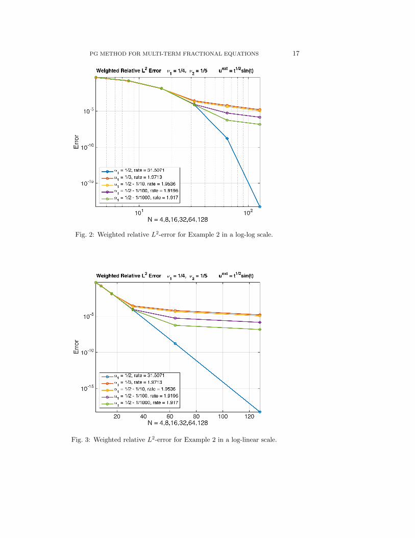
1/2 sin(t), and we observe exponentialconvergence of the method for this example as shown in Figure 3.


Fig. 2: Weighted relative L


Fig. 3: Weighted relative L

2-error for Example 2 in a log-linear scale.


4.3. Example 3. We repeat Example 2 in the case where only the forcing func-tion f(t) is given, and we have chosen f(t) = t

5 so that u satisfies the equation

0

D1/4t u(t) +

0

D1/5t u(t) = t

5

,

u(0) = 0.(76)

The solutions for N = {3, 4, 5, 6} are plotted below in addition to the referencesolution computed with N = 128. We use this reference solution to compute theweighted relative L

2 error in Figure 4.

Fig. 4: Plots of computed solutions with N = {3, 4, 5, 6}, ↵1

= 1/2, and N = 128as the reference solution. In this range, the solution for N = 6 coincides with thereference solution.

4.4. Example 4. In Example 4, we solve the two-term FIVP

0

D4/5t u(t) +

0

D1/2t u(t) = f(t), t 2 (0,+1)

u(0) = 0.(77)


ext(t) = 5t7/2 + 4t2 + t

5/3. We believe this to be an

interesting example because the optimal value of ↵1

is not clear. Using our set ofbasis functions to approximate this solution will not allow us to capture the resultexactly in only a few terms as before, since there are two terms with di↵erent orderfractional singularities at t = 0.

As shown in Figure 6, the approximation using ↵

1

= 1/2 seems to give the bestapproximation to the fabricated solution after the first few values of N , although theasymptotic convergence rate is slower than for the other tested values. The ↵

1

withthe fastest convergence rate of those tested is ↵

1

= 1/6.


Fig. 5: Weighted relative L2-error for Example 3 with respect to the reference solutioncomputed using N = 128 and ↵

1

= 1/2.




4.5. Example 5. To demonstrate that we can also solve equations with a largernumber of terms with high accuracy, we solve the fifty-term FIVP:

50

X

i=1

0

D⌫it u(t) = f(t), t 2 (0,+1)

u(0) = 0,

(78)

where each ⌫i 2 [0,m], with m 1. We choose the parameters as

⌫i =(i� 1)m

K � 1, K = 50, m =

11

12.(79)


ext(t) = t

2+1/4 to plot the weighted relative L

2 errorin Figure 7.



For this example, we also computed the condition numbers of the sti↵ness matricesresulting from the di↵erent values of ↵

1

. In Table 1, we observe that the conditionnumbers in our examples are approximately O(N).


N ↵

1

= 1

4

↵

1

= 1

4

� 1

10

↵

1

= 1

4

� 1

100

↵

1

= 1

2

↵

1

= 2

3

4 2.4325 2.2840 2.4152 2.9990 3.49638 3.9999 3.5478 3.9490 5.6683 7.234916 6.9501 5.7990 6.8199 11.4541 16.145432 12.5912 9.8565 12.2769 24.3153 38.068764 23.5561 17.2719 22.8183 53.5526 93.4535128 45.1956 31.0068 43.4901 121.3111 236.4697

Table 1: Condition numbers of the sti↵ness matrices S in the fifty-term equationfor di↵erent values of the tuning parameter ↵

1

.

In order to compare timings of the method for di↵erent values of K, we timedour PG method solving the equation in Example 5 for K = 2, 10, and 50, where theorders ⌫i are defined using the formula in (79). In Figure 8, we show the timings inactual seconds for N = 1, 2, 3, ..., 30, along with a best-fit line. The timings include

the computation of the load vector ~

f and inverting the linear system to solve forthe coe�cients ~a. As N increases, we also increase the number of quadrature points

used for computing ~

f to maintain the desired level of accuracy. These timings werecollected with Mathematica using a 3 GHz Intel Core i7 processor.

5. Application to distributed order equations. Multi-term fractional dif-ferential equations have been used in combination with a quadrature rule to solvedistributed order di↵erential equations of the form

Z m

0

g(r)0

Drtu(t) dr = f(t),(80)

where the integral on the left hand side is called the distributed order derivative. Thefunction g(r) that appears in the integrand is a distribution where the argument r

corresponds to the order of the fractional derivative. This function must be integrableon [0,m] and satisfy the property g(r) � 0 for all r 2 [0,m].

5.1. Discretized distributed order equation. The idea for solving this equa-tion using multi-term fractional di↵erential equations was proposed by Diethelm andFord [26], where they applied trapezoidal quadrature to the integral in (80) to derive alinear multi-term equation in a bounded interval with constant coe�cients, and thenapplied a finite di↵erence method to solve the distributed order equation. This appli-cation highlights the usefulness of algorithms, which can e�ciently solve multi-termequations with a high number of terms, as may be necessary to decrease the error dueto the quadrature.

For our numerical experiments, we applied the Gauss-Legendre quadrature rule,which has been shown to be spectrally accurate for this setting in the paper byKharazmi et al. [37]. This is demonstrated in Figures 9 and 10.

We are interested in solving the distributed order fractional di↵erential equationon the half line:

Z m

0

g(r)0

Drtu(t) dr = f(t), t 2 (0,+1)

u(0) = 0,

(81)


(a) Two-term equation. (b) Ten-term equation.

(c) Fifty-term equation.

Fig. 8: Timings in actual seconds for the equation from Example 5 with (a) K = 2,(b) K = 10, and (c) K = 50.

where m 2 [0, 1] and0

Drt [·] represents a Riemann-Liouville fractional derivative.

We apply Gauss-Legendre quadrature to the left hand side of (81) side to get themulti-term FIVP:

KX

i=1

wig(⌫i)0D⌫it u(t) ⇡ f(t), t 2 (0,+1)

u(0) = 0,

(82)

where K is the number of quadrature nodes {⌫i} and the weights of the quadraturerule are represented by {wi}Ki=1

. Recall that we approximate the solution to themulti-term equation as

u(t) ⇡ uN (t) =NX

n=1

an�↵1,1n (t),(83)

where

�

↵1,1n (t) := t

↵1L

(↵1)

n�1

(t),(84)


where L

(↵1)

n�1

(t) is the associated Laguerre polynomial of order n� 1.We integrate against the test functions

�

↵2,2k (t) := e

�tL

(↵2)

k�1

(t)(85)

where ↵

2

= ↵

1

� ⌫

1

. Then the variational form for the Petrov-Galerkin method isgiven by

Z 1

0

�

↵2,2k (t)

KX

i=1

wig(⌫i)0D⌫it

NX

n=1

an�↵1,1n (t)

!

drdt =

Z 1

0

f(t)�↵2,2k (t)dt

=: fk.

(86)

Next, we apply fractional integration by parts and the properties of the GALFs asdescribed above:

NX

n=1

an�(n+ ↵

1

)

�(n)

"

w

1

g(⌫1

)�kn +KX

i=2

wig(⌫i)

Z 1

0

e

�tLn�1

(t)L(⌫i�⌫1)

k�1

(t) dt

#

= fk.

(87)

It remains to solve the linear system

S~a = ~

f(88)

for the vector of coe�cients ~a using the factorization methods as described above,where the sti↵ness matrix S is given by

Skn = w

1

g(⌫1

)�kn +KX

i=2

wig(⌫i)

Z 1

0

e

�tLn�1

(t)L(⌫i�⌫1)

k�1

(t) dt.(89)

5.2. Numerical results for distributed order equations. We present con-vergence results of our PG method and Gauss-Legendre quadrature applied to thedistributed order equation (81). The distribution functions g(r) are chosen to besmooth on the interval [0,m] where m < 1.

5.2.1. Example 6. In this example, we choose the fabricated solution to bethe smooth function u

ext(t) = t

3 and the distribution function to be g(r) = �(4 �r) sinh(r). Given these choices, we find that the right hand side function f(t) is

Z m

0

g(r)0

Drtu

ext(t) dr =t

3�m(tm � cosh(m)� log(t) sinh(m))

(log(t))2 � 1=: f(t).(90)

The plateaus in the error in Figure 9 correspond to the error for the Gauss-Legendre rule, and we reach machine precision with (a) K = 10 and (b) K = 6quadrature points, where in (a) we use m = 9/10 and in (b) we use m = 1/10. Wechoose the tuning parameter for the PG method to be ↵

1

= 1. The weighted relativeL

2 error for both quadrature rules is plotted in Figure 9.


(a) m = 9/10 (b) m = 1/10

Fig. 9: (a) Weighted relative L

2-error for Gauss-Legendre quadrature and our PGmethod applied to Example 6 with m = 9/10, where K is the number of quadraturepoints used. (b) Weighted relative L

2-error for Example 6 with m = 1/10.

5.2.2. Example 7. Now we test a non-smooth example, where the fabricatedsolution is u

ext(t) = t

� with � = 2 + 1/3 and the distribution function is g(r) =�(1+��r)�(�+1)

. Then the right hand side function f(t) is

Z m

0

g(r)0

Drtu

ext(t) dr =t

��m(tm � 1)

log(t)=: f(t).(91)

We choose the tuning parameter for the PG method to be ↵

1

= 1/3.The weighted relative L

2 error for m = 9/10, 1/2 and 1/10 is plotted in Figure10.

(a) m = 9/10 (b) m = 1/10

Fig. 10: (a) Weighted relative L

2 error for Example 7 with m = 9/10. (b) Weightedrelative L

2 error for Example 7 with m = 1/10.


6. Summary and Conclusion. We have presented a Laguerre Petrov-Galerkinspectral method for solving multi-term fractional initial value problems on the halfline with linear complexity, which is a significant reduction from the cubic complexityrequired for existing spectral methods.

The key element of this work that resulted in the reduced complexity was ourderivation of a factorization of the discretized system of equations, in which we tookadvantage of the special structure of the generalized associated Laguerre functions.Our method also has the unusual advantage that it is applicable without modificationto multi-term equations that include a reaction term, as the resulting mass matrix hasthe same special structure that allows us to invert the sti↵ness matrices e�ciently. Wehave demonstrated the e↵ectiveness of our method by solving a 50-term equation anddistributed order equations, which were discretized by a Gauss-Legendre quadraturerule. Our numerical results highlight the sensitivity of the convergence rate to thetunable parameter ↵

1

, while we were able to achieve spectral convergence whether ornot the parameter was chosen optimally.

In the future, we will examine methods of analyzing our PG method and deriveerror estimates in the weighted relative L

2-norm to prove the spectral convergence ofthe method demonstrated in the numerical results sections.

REFERENCES

[1] H. Brunner. Collocation methods for Volterra integral and related functional di↵erential equa-tions, volume 15. Cambridge University Press, Cambridge, UK, 11 2004.

[2] L.M. Delves and J.L. Mohamed. Computational methods for integral equations. CambridgeUniversity Press, Cambridge, UK, 12 1985.

[3] I. Podlubny. Fractional di↵erential equations. Academic Press, Inc., San Diego, CA, 1999.[4] J.T. Edwards, N. J. Ford, and A. C. Simpson. The numerical solution of linear multi-term frac-

tional di↵erential equations: Systems of equations. Journal of Computation and AppliedMathematics, 148:401–418, 2002.

[5] C. Celik and M. Duman. Crank-Nicolson method for the fractional di↵usion equation with theRiesz fractional derivative. J. Comput. Phys., 231:1743–1750, 2012.

[6] M. Chen and W. Deng. Fourth order accurate scheme for the space fractional di↵usion equa-tions. SIAM J. Numer. Anal., 52:1418–1438, 2014.

[7] H. Ding, C. Li, and Y. Chen. High-order algorithms for Riesz derivative and their applications.Abstr. Appl. Anal., 2013.

[8] W. Deng. Finite element method for the space and time fractional Fokker-Planck equation.SIAM J. Numer. Anal., 47:204–226, 2008/09.

[9] V.J. Ervin and J.P. Roop. Variational solution of fractional advection dispersion equationson bounded domains in Rd. Numer. Methods Partial Di↵erential Equations, 23:256–281,2007.

[10] M. Zayernouri, M. Ainsworth, and G. E. Karniadakis. A unified Petrov-Galerkin spectralmethod for fractional PDEs. Computer Methods in Applied Mechanics and Engineering,283:1545–1569, 2015.

[11] M. Zayernouri and G. E. Karniadakis. Exponentially accurate spectral and spectral elementmethods for fractional ODEs. Journal of Computational Physics, 257:460–480, 2014.

[12] M. Zayernouri and G. E. Karniadakis. Fractional Sturm–Liouville eigen-problems: Theory andnumerical approximation. Journal of Computational Physics, 252:495–517, 2013.

[13] M. Zayernouri, M. Ainsworth, and G. E. Karniadakis. Tempered fractional Sturm–Liouvilleeigen problems. SIAM Journal on Scientific Computing, 37(4):A1777–A1800, 2015.

[14] M. Zayernouri and G. E. Karniadakis. Fractional spectral collocation method. SIAM Journalon Scientific Computing, 36(1):A40–A62, 2014.

[15] M. Zayernouri and G. E. Karniadakis. Discontinuous spectral element methods for time-andspace-fractional advection equations. SIAM Journal on Scientific Computing, 36(4):B684–B707, 2014.

[16] H. Khosravian-Arab, M. Dehghan, and M.R. Eslahchi. Fractional Sturm-Liouville boundaryvalue problems in unbounded domains: Theory and applications. Journal of ComputationalPhysics, 229:526–560, 2015.


[17] D. Gottlieb and S. A. Orszag. Numerical analysis of spectral methods: Theory and applications,volume 26. SIAM, 1977.

[18] Z. Zhang, F. Zeng, and G. E. Karniadakis. Optimal error estimates of spectral Petrov-Galerkinand collocation methods for initial value problems of fractional di↵erential equations. SIAMJ. Numer. Anal., 53:2074–2096, 2015.

[19] D. Baleanu, A.H. Bhrawy, and T.M. Taha. A modified generalized Laguerre spectral methodfor fractional di↵erential equations on the half line. Abstract and Applied Analysis, 2013.

[20] A.H. Bhrawy, D. Baleanu, and L.M. Assas. E�cient generalized Laguerre spectral methods forsolving multi-term fractional di↵erential equations on the half line. Journal of Vibrationand Control, 2013.

[21] M. Zheng, F. Liu, V. Anh, and I. Turner. A high order spectral method for the multi-termtime-fractional di↵usion equation. Applied Mathematical Modelling, 40, 2016.

[22] Y. Zhao, Y. Zhang, F. Liu, I. Turner, Y. Tang, and V. Anh. Convergence and superconver-gence of a fully-discrete scheme for multi-term time fractional di↵usion equations. AppliedMathematical Modelling, 2016.

[23] F. Liu, M.M. Meerschaert, R. McGough, P. Zhuang, and Q. Liu. Numerical methods for solvingthe multi-term time fractional wave equations. Fractional Calculus and Applied Analysis,16(1):9–25, 2013.

[24] H. Ye, F. Liu, I. Turner, V. Anh, and K. Burrage. Series expansion solutions for the multi-termtime and space fractional partial di↵erential equations in two and three dimensions. Eur.Phys. J., Special Topics, 222:1901–1914, 2013.

[25] C. Ming, F. Liu, L. Zheng, I. Turner, and V. Anh. Analytical solutions of multi-term timefractional di↵erential equations and application to unsteady flows of generalized viscoelasticfluid. Computers and Mathematics with Applications, 2016.

[26] K. Diethelm and N. J. Ford. Numerical analysis for distributed-order di↵erential equations. J.of Comp. and App. Math., 225, 2009.

[27] T. M. Atanackovic, M. Budincevic, and S. Pilipovic. On a fractional distributed-order oscillator.Journal of Physics A: Mathematical and General, 38:6703–6713, 2005.

[28] M. Naghibolhosseini. Estimation of outer-middle ear transmission using DPOAEs andfractional-order modeling of human middle ear. PhD thesis, City University of New York,NY., 2015.

[29] M. Caputo. Distributed order di↵erential equations modelling dielectric induction and di↵usion.Fract. Calc. Appl. Anal., 4:421–442, 2001.

[30] M. Caputo. Di↵usion with space memory modelled with distributed order space fractionaldi↵erential equations. Ann. Geophys., 46:223–234, 2003.

[31] I.M. Sokolov, A.V. Chechkin, and J. Klafter. Distributed order fractional kinetics. Acta Phys.Pol. B, 35:1323–1341, 2004.

[32] S.G. Samko, A.A. Kilbas, and O.I. Marichev. Fractional integrals and derivatives. Gordon andBreach Science Publishers, Yverdon, 1993.

[33] X. Li and C. Xu. A space-time spectral method for the time fractional di↵usion equation.SIAM Journal on Numerical Analysis, 47(3):2108–2131, 2009.

[34] P.G. Martinsson, V. Rokhlin, and M. Tygert. A fast algorithm for the inversion of generalToeplitz matrices. Computers and Mathematics with Applications, 50:741–752, 2005.

[35] J. Shen, T. Tang, and L.-L. Wang. Spectral Methods: Algorithms, Analysis and Applications.Springer, 8 2011.

[36] J. Hesthaven, S. Gottlieb, and D. Gottlieb. Spectral Methods for Time-Dependent Problems.Cambridge University Press, Cambridge, UK, 2007.

[37] E. Kharazmi, M. Zayernouri, and G. E. Karniadakis. Petrov-Galerkin and spectral collocationmethods for distributed order di↵erential equations. arXiv preprint arXiv:1604.08650,2016.

Documents

A PETROV-GALERKIN SPECTRAL METHOD OF LINEAR … · A PETROV-GALERKIN SPECTRAL METHOD OF LINEAR COMPLEXITY FOR FRACTIONAL MULTI-TERM ODES ... The Rodrigues formula for these ... solutions