Embed Size (px)
DESCRIPTION
The paper proposes a post-Keynesian framework to explain Tobin’s q behaviour in the long run. The theoretical basis is informed by the Cambridge corporate model originally proposed by Kaldor (1966), which is reinterpreted here as a theory for q.
Citation preview
A Post-Keynesian Theory for Tobin’s q in a Stock-Flow
Consistent Framework
Javier López Bernardo, Engelbert Stockhammer and Félix López Martínez
July 2015
PKSG
Post Keynesian Economics Study Group
Working Paper 1509
This paper may be downloaded free of charge from www.postkeynesian.net
© Javier López Bernardo, Engelbert Stockhammer and Félix López Martínez
Users may download and/or print one copy to facilitate their private study or for non-commercial research and
may forward the link to others for similar purposes. Users may not engage in further distribution of this material
or use it for any profit-making activities or any other form of commercial gain.
A Post-Keynesian Theory for Tobin’s q in a Stock-Flow
Consistent Framework
Abstract: The paper proposes a post-Keynesian framework to explain Tobin’s q behaviour in
the long run. The theoretical basis is informed by the Cambridge corporate model originally
proposed by Kaldor (1966), which is reinterpreted here as a theory for q. The core of the
‘Kaldorian q theory’ is a negative long-run relation between q and growth rates, a negative
relation between q and propensities to consume, and the fact that q can be different from 1 in
the long-run equilibrium. We generalise this model through a medium-scale Stock-Flow
Consistent (SFC) model, which introduces important post-Keynesian aspects missing in the
Kaldorian model, such as endogenous money, a financial system and inflation. We extend the
model to include a more realistic treatment of firms’ financial structure decisions and allow
the interdependence between these decisions and dividend policy. Numerical simulations
confirm that the original Kaldorian relations between q and growth rates and propensities to
consume hold, but unlike the original model, in our model q is not independent of how firms
finance their investment. We also confirm the possibility of q being different from 1 in the
long-run. Finally, we contrast this ‘post-Keynesian q theory’ with the Miller-Modigliani
dividend irrelevance proposition and the neoclassical investment and financial theory. It is
shown that its validity depends crucially on the value taken by q: for q values different from 1
the proposition will not hold and dividend policy will be relevant for equity valuation.
Therefore, post-Keynesian q theory stands against the main predictions of mainstream
finance and constitutes an alternative for developing a macroeconomic theory for equity
markets.
Keywords: Tobin’s q, post-Keynesian macroeconomic theory, stock-flow consistent models,
Cambridge corporate models, Miller-Modigliani dividend irrelevance proposition
JEL classifications: E12, E22, E44, G10, O42
Acknowledgements. We gratefully acknowledge helpful comments and suggestions by Paul
Auerbach, Malcolm Sawyer, Dimitris Sotiropoulos, Rafael Wildauer and participants of the
12th Conference, Developments in Economics Theory and Policy, held in Bilbao, June 2015.
However, none of them are responsible for the final views expressed here. Javier López also
acknowledges financial support by the Ramón Areces Foundation (Madrid).
Javier López Bernardo, Kingston University London, KT1 2EE, Kingston upon Thames, UK;
email: [email protected]
PKSG A post-Keynesian theory for Tobin’s q
July 2015 Page | 1 Bernardo, Stockhammer and Martínez
1. Introduction
Tobin’s q is defined as the ratio of the ‘going price in the market for exchanging existing assets’
to their ‘replacement or reproduction cost’ (Tobin & Brainard, 1977).1 Since the seminal works
of Brainard and Tobin (Brainard & Tobin, 1968; Tobin, 1969; Tobin & Brainard, 1977), Tobin’s q
has become an important theoretical construct widely used both by financial practitioners to
assess current stock market conditions (Montier, 2014a; Smithers, 2009) and by academics,
who have used q as the main explanatory variable in investment functions (Hayashi, 1982).
However, none of the two groups have offered an explanation of the movements of q through
time: the first group has usually assumed mean-reversion for the q series (with no strong
theoretical justification) while the second has been more interested in the role of q as an
exogenous variable, not as an endogenous one.
The present paper offers an alternative macroeconomic vision of q based on the ‘Cambridge
corporate model’ developed by Kaldor and others in the 1960s and 1970s (Kaldor, 1966;
Marris, 1972; Moore, 1975; Moss, 1978). The Cambridge corporate model was originally
proposed as a solution for the Harrod-Domar knife-edge dilemma, where equity valuation (not
technology, as in the neoclassical framework, nor income distribution, as in the original
Cambridge model) was the adjusting variable that brought overall savings and investment in
equilibrium. This model can be reinterpreted as a macroeconomic theory for the valuation of
equity markets – i.e. as a theory explaining q. This new interpretation offers two important
conclusions: first, it finds a negative long-run relationship at the macroeconomic level between
growth rates and valuation ratios; this is in contrast to firm-level equity valuation models (e.g.
dividend, residual income and free-cash-flow discounted models), which suggest the opposite.2
Second, the causality goes from investment and animal spirits to q, whereas the neoclassical
model (Hayashi, 1982) stresses the importance of q on investment decisions.3 This simple
Kaldorian framework has been able to explain remarkably well the experience of the last
decades in developed countries, where lower growth rates have been associated with higher
valuation ratios. However, the Kaldorian framework has at least two important shortcomings:
first, it is based on a real economy framework without money where equities are the only
financial asset (Davidson, 1968; Kregel, 1985) and, second, the modelling of firms’ financing
decisions is simplistic in that it assumes fixed dividend payout and share issue ratio. In other
words, dividend and financing decisions are made independent of financial market conditions.
This paper generalises and extends the Kaldorian model to address these shortcomings. This
will be done through a medium-scale SFC model, which allows for a more sophisticated
1 In fact, first person to propose this ratio at the macroeconomic level was Kaldor (1966), who called it the ‘valuation ratio’. In this chapter, the words ‘Tobin’s q’ and ‘valuation ratio’ will be used interchangeably. 2 The insight that higher growth rates lead to lower valuation ratios has profound implications both for policy makers and market participants. The importance of market valuations for policy makers have been argued in length in Smithers (2009), who argues that central bankers should pay more attention to financial market valuations and not exclusively price inflation. For market participants, it is useful to have an idea whether markets are ‘expensive’ or not. However, at the macro level, traditional fundamental equity valuation methods applied to the valuation of whole indices will not work if the Kaldorian insight applies – because these discounted cash-flows methods will tell you that higher growth rates should lead to higher valuations. 3 Although Tobin and Brainard did not develop formally this reverse causation issue, they briefly hinted at this dependence of q on investment decisions; ‘We agree that q’s are partly endogenous variables, that investments can influence q’s as well as vice versa, and that the lags between exogenous changes in q and investment could be “long and variable”’ (Tobin & Brainard, 1990, p. 548).
PKSG A post-Keynesian theory for Tobin’s q
July 2015 Page | 2 Bernardo, Stockhammer and Martínez
treatment of the financial aspects of the economy with a richer asset-liability structure. Our
model is a generalisation because it contains Kaldor’s key behavioural function but also
includes some realistic features missing in the original model, such as endogenous money,
financial markets, cost-push inflation, corporate leverage and fiscal and monetary policy. We
thus address the first shortcoming. In terms of behavioural assumptions, the model follows
established post-Keynesian theory, but we deviate in one important aspect. In contrast to the
Kaldorian model and to the standard SFC literature (Godley & Lavoie, 2007; Dos Santos &
Zezza, 2008; Le Heron & Mouakil, 2008; Van Treeck, 2008), we consider financing and dividend
policy decisions as interdependent following Gordon (1992, 1994). We have endogenous
dividend payout and share issuance and thus address the second shortcoming.
The aim of the model is to demonstrate that post-Keynesian theory, using a reasonable set of
assumptions, can offer a robust theoretical explanation for the behaviour of q over the long-
run. While our SFC model features both short-term and long-term dynamics, our focus is, like
Kaldor’s, on long-run steady-state positions. Our modelling of short run dynamics remains
minimalistic; in particular we bypass all the interesting asset price dynamics highlighted by the
Minskyan theory of financial markets and behavioural finance (Thaler, 2005).4 We do so not
because these issues would not be important – indeed they are – but because we argue that
even in steady growth equilibrium without speculation or any other specific behavioural bias,
post-Keynesian theory offers a distinct explanation of q.
The main findings of our post-Keynesian model are as follows. First, the original two long-run
relationships of the Kaldorian model, between q and growth rates and q and propensities to
consume, hold. Second, in contrast to the Kaldorian model, simulations show that the way
investment is financed matters, not only for q, but also for output, employment and prices.
Finally, as in Kaldor’s, the level of q does not tend to 1 even in the long-run, contradicting thus
the neoclassical q theory where the equilibrium level of q is 1. This last finding has far-reaching
consequences for the Miller-Modigliani (M&M) dividend irrelevance proposition (Miller &
Modigliani, 1961), which states that the value of a corporation is independent from its
dividend policy. Although the theory was originally under attack by corporate finance theorists
(Lintner, 1962; Gordon, 1963; Walter, 1963), now it is commonplace in finance and has been
widely used as a micro-foundation for many neoclassical macro models.5 We show that the
M&M dividend proposition will only hold when q is equal to 1, a condition that in our post-
Keynesian model will be only fulfilled by chance.
The structure of the paper is as follows. Section 2 reviews the literature on q, with special
emphasis on the theoretical literature and on the main features of the Cambridge corporate
models. Section 3 presents a post-Keynesian SFC model and the simulations conducted to
study its behaviour. Section 4 explains the implications of the post-Keynesian q theory for the
validity of the M&M dividend proposition. Section 5 concludes.
4 For a discussion of a possible research agenda in common between post-Keynesian economics and behavioural finance, see Jefferson & King (2010). 5 This is the case in most real-business cycle and new-Keynesian models. See, for instance, Christiano et al. (2005) and Smets & Wouters (2007). In these models, the institutional setup is irrelevant (it does not matter who owns what), so that capital structure (and dividend policy) is irrelevant. In addition, no clear picture of the role of financial intermediaries in the system is provided.
PKSG A post-Keynesian theory for Tobin’s q
July 2015 Page | 3 Bernardo, Stockhammer and Martínez
2. Literature review
2.1 Tobin’s q in the neoclassical framework
Keynes (1936, chp. 12) admitted that ‘the daily revaluations of the stock exchange[...]
inevitably exert a decisive influence on the rate of current investment. For there is no sense in
building up a new enterprise at a cost greater than that at which a similar existing enterprise
can be purchased [...] if it can be floated off on the Stock Exchange at an immediate profit’
(1936, chp. 12). Brainard and Tobin (1968) and Tobin (1969) took up Keynes’s idea in a formal
model; the latter was an extension of the original Hicks IS-LM model with an LM curve
depending on a vector of asset prices rather than on a single interest rate, while the former
was one of the first contributions in dealing with macro models embedded in a rigorous
accounting structure and can be regarded as an early forerunner of the SFC methodology.
Another interpretation of Keynes’s idea was offered by Minsky (2008), whose framework is
similar to Tobin’s in that investment depends on the difference between the demand price and
the supply price of capital goods.6
In neoclassical theory, as in Brainard and Tobin’s seminal papers, q plays the main role in
investment decisions, but uses a more restricted microeconomic rational behaviour setting.7
This implementation was developed by Lucas & Prescott (1971), Yoshikawa (1980) and Hayashi
(1982), and since then q has become the ‘preferred theoretical description of investment’
(Fischer & Merton, 1984, p.29) in a neoclassical framework and is featured as such in advanced
textbooks (Carlin & Soskice, 2006; Romer, 2012). One reason for its success is that the model
can be derived from the maximising behaviour of a single representative firm operating in
competitive markets and facing adjustment costs. Such adjustment costs can be either internal
(installation and other costs) or external (new investment induced by a higher level of q bids
up the price of capital goods), but the workings of the theory are the same in both cases
(Romer, 2012, p. 408). The relevant q for the neoclassical theory of investment is marginal q,
that is, the ratio of the market value of a marginal unit of capital to its replacement cost.8 The
equilibrium value for q is 1; if, for whatever reason, the actual value is above that level, wealth-
maximising firms will find profitable investment projects and then will push down the marginal
efficiency of capital (i.e. the rate of profit), given the assumption of a production function with
decreasing marginal factor returns.
There have been several theoretical criticisms to this framework. First, marginal q is an
unobservable variable, so ‘[t]he managerial investment decision-making process cannot
possibly be guided by an unobservable variable’ (Crotty, 1990, p. 538, emphasis in the
original). Second, perfect capital markets are assumed, and shareholders and managers are
6 For a discussion of the differences between Minsky and Brainard and Tobin’s framework, see Crotty (1990) and Palley (2001). 7 However, Brainard and Tobin’s framework is quite different from the neoclassical one. As they admit: ‘We are so far from being thorough-going neoclassicals that we are quite comfortable in believing that corporate managers […] respond to market noise and are in any case sluggish in responding to the arbitrage opportunities of large deviations of “q” from par’ (Tobin & Brainard, 1990, p. 548). Furthermore, Tobin (1984, pp. 6–7) expressed serious reservations about the ‘efficiency of financial markets’, citing approvingly Keynes’s idea of markets driven by non-informed, herding behaviour. 8 Under constant returns on the adjustment costs, it can be shown that marginal and average q coincide (Hayashi, 1982). Moreover, other influences such as monopoly power, downward-sloping product demand curves and a large share of dated capital can produce discrepancies between the marginal and the average q. See Romer (2012, p. 415).
PKSG A post-Keynesian theory for Tobin’s q
July 2015 Page | 4 Bernardo, Stockhammer and Martínez
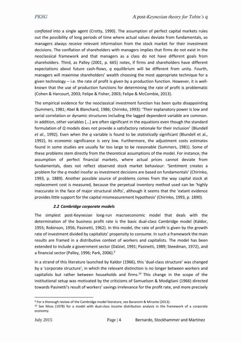
conflated into a single agent (Crotty, 1990). The assumption of perfect capital markets rules
out the possibility of long periods of time where actual values deviate from fundamentals, so
managers always receive relevant information from the stock market for their investment
decisions. The conflation of shareholders with managers implies that firms do not exist in the
neoclassical framework and that managers as a class do not have different goals from
shareholders. Third, as Palley (2001, p. 665) notes, if firms and shareholders have different
expectations about future cash-flows, q equilibrium will be different from unity. Fourth,
managers will maximise shareholders’ wealth choosing the most appropriate technique for a
given technology – i.e. the rate of profit is given by a production function. However, it is well-
known that the use of production functions for determining the rate of profit is problematic
(Cohen & Harcourt, 2003; Felipe & Fisher, 2003; Felipe & McCombie, 2013).
The empirical evidence for the neoclassical investment function has been quite disappointing
(Summers, 1981; Abel & Blanchard, 1986; Chirinko, 1993): ‘Their explanatory power is low and
serial correlation or dynamic structures including the lagged dependent variable are common.
In addition, other variables [...] are often significant in the equations even though the standard
formulation of Q models does not provide a satisfactory rationale for their inclusion’ (Blundell
et al., 1992). Even when the q variable is found to be statistically significant (Blundell et al.,
1992), its economic significance is very low. Furthermore, the adjustment costs estimates
found in some studies are usually far too large to be reasonable (Summers, 1981). Some of
these problems stem directly from the theoretical assumptions of the model. For instance, the
assumption of perfect financial markets, where actual prices cannot deviate from
fundamentals, does not reflect observed stock market behaviour: ‘Sentiment creates a
problem for the q model insofar as investment decisions are based on fundamentals’ (Chirinko,
1993, p. 1889). Another possible source of problems comes from the way capital stock at
replacement cost is measured, because the perpetual inventory method used can be ‘highly
inaccurate in the face of major structural shifts’, although it seems that the ‘extant evidence
provides little support for the capital mismeasurement hypothesis’ (Chirinko, 1993, p. 1890).
2.2 Cambridge corporate models
The simplest post-Keynesian long-run macroeconomic model that deals with the
determination of the business profit rate is the basic dual-class Cambridge model (Kaldor,
1955; Robinson, 1956; Pasinetti, 1962). In this model, the rate of profit is given by the growth
rate of investment divided by capitalists’ propensity to consume. In such a framework the main
results are framed in a distributive context of workers and capitalists. The model has been
extended to include a government sector (Dalziel, 1991; Pasinetti, 1989; Steedman, 1972), and
a financial sector (Palley, 1996; Park, 2006).9
In a strand of this literature launched by Kaldor (1966), this ‘dual-class structure’ was changed
by a ‘corporate structure’, in which the relevant distinction is no longer between workers and
capitalists but rather between households and firms.10 This change in the scope of the
institutional setup was motivated by the criticisms of Samuelson & Modigliani (1966) directed
towards Pasinetti’s result of workers’ savings irrelevance for the profit rate, and more precisely
9 For a thorough review of the Cambridge model literature, see Baranzini & Mirante (2013). 10 See Moss (1978) for a model with dual-class income distribution analysis in the framework of a corporate economy.
PKSG A post-Keynesian theory for Tobin’s q
July 2015 Page | 5 Bernardo, Stockhammer and Martínez
to what they regarded as the assumption of ‘the existence of identifiable classes of capitalists
and workers with “permanent membership” – even as rough first approximation’ (Samuelson
& Modigliani, 1966, p. 271). In his rejoinder, Kaldor (1966, p.310) considered the high
propensity to save out of profits ‘something which attaches to the nature of business income,
and not to the wealth (or other peculiarities) of the individuals who own property.’
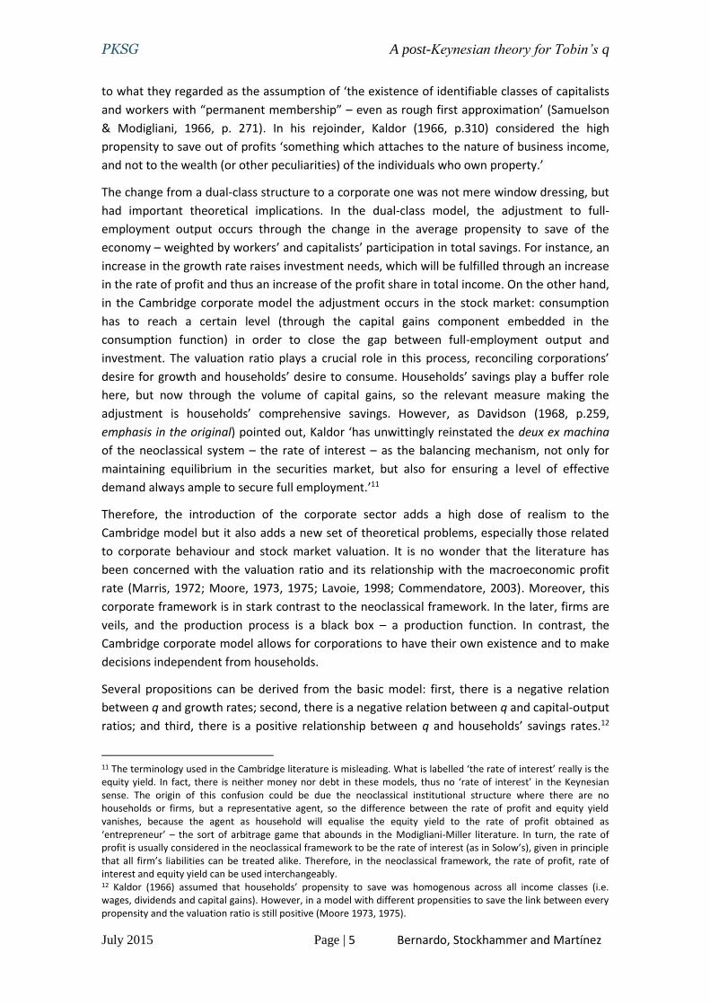
The change from a dual-class structure to a corporate one was not mere window dressing, but
had important theoretical implications. In the dual-class model, the adjustment to full-
employment output occurs through the change in the average propensity to save of the
economy – weighted by workers’ and capitalists’ participation in total savings. For instance, an
increase in the growth rate raises investment needs, which will be fulfilled through an increase
in the rate of profit and thus an increase of the profit share in total income. On the other hand,
in the Cambridge corporate model the adjustment occurs in the stock market: consumption
has to reach a certain level (through the capital gains component embedded in the
consumption function) in order to close the gap between full-employment output and
investment. The valuation ratio plays a crucial role in this process, reconciling corporations’
desire for growth and households’ desire to consume. Households’ savings play a buffer role
here, but now through the volume of capital gains, so the relevant measure making the
adjustment is households’ comprehensive savings. However, as Davidson (1968, p.259,
emphasis in the original) pointed out, Kaldor ‘has unwittingly reinstated the deux ex machina
of the neoclassical system – the rate of interest – as the balancing mechanism, not only for
maintaining equilibrium in the securities market, but also for ensuring a level of effective
demand always ample to secure full employment.’11
Therefore, the introduction of the corporate sector adds a high dose of realism to the
Cambridge model but it also adds a new set of theoretical problems, especially those related
to corporate behaviour and stock market valuation. It is no wonder that the literature has
been concerned with the valuation ratio and its relationship with the macroeconomic profit
rate (Marris, 1972; Moore, 1973, 1975; Lavoie, 1998; Commendatore, 2003). Moreover, this
corporate framework is in stark contrast to the neoclassical framework. In the later, firms are
veils, and the production process is a black box – a production function. In contrast, the
Cambridge corporate model allows for corporations to have their own existence and to make
decisions independent from households.
Several propositions can be derived from the basic model: first, there is a negative relation
between q and growth rates; second, there is a negative relation between q and capital-output
ratios; and third, there is a positive relationship between q and households’ savings rates.12
11 The terminology used in the Cambridge literature is misleading. What is labelled ‘the rate of interest’ really is the equity yield. In fact, there is neither money nor debt in these models, thus no ‘rate of interest’ in the Keynesian sense. The origin of this confusion could be due the neoclassical institutional structure where there are no households or firms, but a representative agent, so the difference between the rate of profit and equity yield vanishes, because the agent as household will equalise the equity yield to the rate of profit obtained as ‘entrepreneur’ – the sort of arbitrage game that abounds in the Modigliani-Miller literature. In turn, the rate of profit is usually considered in the neoclassical framework to be the rate of interest (as in Solow’s), given in principle that all firm’s liabilities can be treated alike. Therefore, in the neoclassical framework, the rate of profit, rate of interest and equity yield can be used interchangeably. 12 Kaldor (1966) assumed that households’ propensity to save was homogenous across all income classes (i.e. wages, dividends and capital gains). However, in a model with different propensities to save the link between every propensity and the valuation ratio is still positive (Moore 1973, 1975).

PKSG A post-Keynesian theory for Tobin’s q
July 2015 Page | 6 Bernardo, Stockhammer and Martínez
Regarding the profit rate, higher growth rates have a positive effect on profit rates, whereas
higher retention ratios and higher new share issues have a detrimental effect on the profit
rate. Finally, higher growth rates have an unequivocal positive effect on the equity yield – both
through higher profit rates and a lower Tobin’s q.
The pair of relationships between q and growth rates, and q and savings rates constitutes the
core of what we call the ‘Kaldorian theory of q’. Despite its simplicity, the model is able to
explain remarkably well the long-run trend of q in, for instance, the US economy and other
developed economies during the last 40 years.13 The evidence shows that the recent higher
level of q (Montier, 2014a; Piketty, 2014, p. 189) has been coupled with lower accumulation
rates and higher propensities to save, the latter due to income redistribution to the top
percentile; these effects, inter alia, are usually associated in the post-Keynesian literature with
the financialisation process (Stockhammer, 2004; Orhangazi, 2008; Van Treeck, 2008).
Moreover, there is nothing in the Kaldorian theory to preclude q from being persistently
different from unity. Admittedly, there have been other factors that have undoubtedly played
a role in the evolution of q, notably the increase in leverage and the change in institutions,
which are not included in the model. But the evidence taken at face value between growth
rates, q and savings rates is in principle favourable to the post-Keynesian theory.
Another remarkable feature of the Kaldorian theory that has gone unnoticed in the post-
Keynesian literature14 is that it reverses the causation compared to neoclassical theory: while
mainstream theory predicts a causal link running from q to investment, the Kaldorian theory
posits a link running from investment to q. While the mainstream theory supports stock
market booms as drivers of corporate investment (q values higher than one), in the Kaldorian
theory such a mechanism is assumed to be irrelevant. The Kaldorian theory features the
Keynesian principle that investment is given by animal spirits, while in the mainstream theory
investment is given by the production function through the law of the one price – the
entrepreneur will carefully equalise the marginal efficiency of capital to the marginal
productivity of capital (rate of profit), the latter given by the production function.
However, there are other, less favourable features in the basic Kaldorian model. There are
problems of omission as well as commission. The problem of omission is that Kaldor offers an
explanation of q based on a model without a proper financial sector. There are not banks,
there is no money and there is only one financial asset. The problem of commission is in the
modelling of firms’ financing decisions and dividend policy. Kaldor assumes that a fixed part of
profits is paid out as dividends and a fixed share of investment is financed by equity issue,
independent of financial market conditions. However, in the real world, the financing decision
and the dividend decision are neither independent nor completely fixed regardless of the state
of capital markets. Moreover, a higher proportion of investment financed through new shares
should lead to lower valuation ratios – given the higher supply of shares. Finally, one would
expect that other factors not included in the model (most notably, corporate leverage,
13 Full disclaimer: all these relationships should be properly understood in a long-run context. 14 See the discussion in the previous section. Post-Keynesians disagree on the neoclassical investment functions (those solely with q as an independent variable), on the grounds that the rationality imposed is absurd (e.g. radical uncertainty and animal spirits) or on the grounds that no quantities (e.g. cash-flows, utilisation) are included. Thus q is not a key determinant of investment. Our point is that investment is a determinant of q.
PKSG A post-Keynesian theory for Tobin’s q
July 2015 Page | 7 Bernardo, Stockhammer and Martínez
inflation, and fiscal and monetary policy) to affect the evolution of q. These issues will be
addressed in the model presented in the next section.
3 A post-Keynesian SFC model for Tobin’s q behaviour
The Cambridge model allows gleaning very general relationships between q and other
macroeconomic variables, but at the cost of simplification. The model presented here depicts a
more sophisticated economic system with post-Keynesian sectoral behaviour. The main post-
Keynesian features are: endogenous money, mark-up pricing, sectors with independent
motivations (especially households, firms and banks) and a theoretical framework that is
demand-led. Because the model presented is too large to be solved analytically, simulations
will be performed to analyse q’s behaviour over time. We are specifically interested in three
sets of shocks that will allow us to evaluate whether the conclusions of the original Kaldorian
model still hold: a change in the growth rate of the economy, a change in households’
propensity to consume and a change in the willingness of corporations to issue new shares.
3.1 The model
The model consists of 56 equations. The three matrices that lay out the full accounting
structure of the model (stocks, flows and price revaluations) can be found in the Appendix.
Except for firms’ financing decisions, no pretension of originality in the behavioural
assumptions is made; rather, the aim is to set up a model based on established aspects of
post-Keynesian theory as far as possible. Given the size of the model, only the main
behavioural equations will be discussed, the full list of equations can be found in the Appendix.
For the sake of convenience, each sector is discussed separately.
Firms’ behaviour
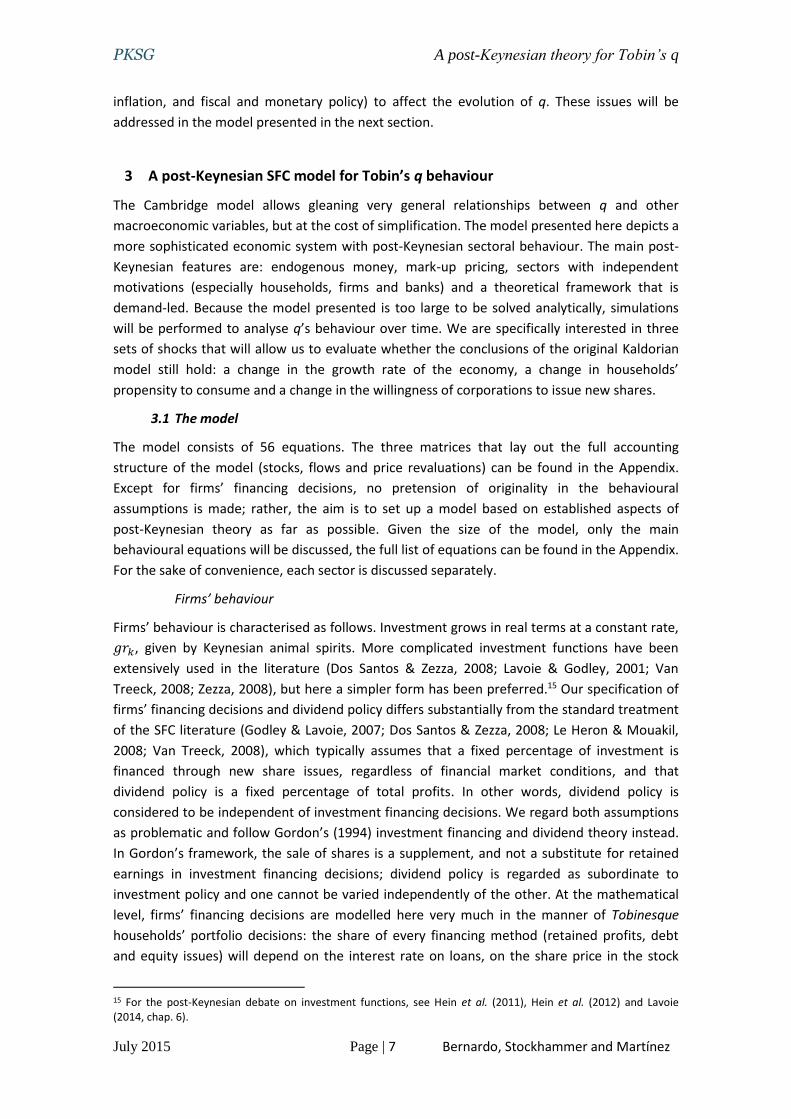
Firms’ behaviour is characterised as follows. Investment grows in real terms at a constant rate,
𝑔𝑟𝑘, given by Keynesian animal spirits. More complicated investment functions have been
extensively used in the literature (Dos Santos & Zezza, 2008; Lavoie & Godley, 2001; Van
Treeck, 2008; Zezza, 2008), but here a simpler form has been preferred.15 Our specification of
firms’ financing decisions and dividend policy differs substantially from the standard treatment
of the SFC literature (Godley & Lavoie, 2007; Dos Santos & Zezza, 2008; Le Heron & Mouakil,
2008; Van Treeck, 2008), which typically assumes that a fixed percentage of investment is
financed through new share issues, regardless of financial market conditions, and that
dividend policy is a fixed percentage of total profits. In other words, dividend policy is
considered to be independent of investment financing decisions. We regard both assumptions
as problematic and follow Gordon’s (1994) investment financing and dividend theory instead.
In Gordon’s framework, the sale of shares is a supplement, and not a substitute for retained
earnings in investment financing decisions; dividend policy is regarded as subordinate to
investment policy and one cannot be varied independently of the other. At the mathematical
level, firms’ financing decisions are modelled here very much in the manner of Tobinesque
households’ portfolio decisions: the share of every financing method (retained profits, debt
and equity issues) will depend on the interest rate on loans, on the share price in the stock
15 For the post-Keynesian debate on investment functions, see Hein et al. (2011), Hein et al. (2012) and Lavoie (2014, chap. 6).
PKSG A post-Keynesian theory for Tobin’s q
July 2015 Page | 8 Bernardo, Stockhammer and Martínez
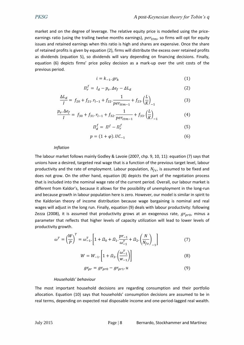
market and on the degree of leverage. The relative equity price is modelled using the price-
earnings ratio (using the trailing twelve months earnings), 𝑝𝑒𝑟𝑡𝑡𝑚, so firms will opt for equity
issues and retained earnings when this ratio is high and shares are expensive. Once the share
of retained profits is given by equation (2), firms will distribute the excess over retained profits
as dividends (equation 5), so dividends will vary depending on financing decisions. Finally,
equation (6) depicts firms’ price policy decision as a mark-up over the unit costs of the
previous period.
𝑖 = 𝑘−1. 𝑔𝑟𝑘 (1)
𝛱𝑟𝑓
= 𝐼𝑑 − 𝑝𝑒 . 𝛥𝑒𝑓 − 𝛥𝐿𝑑 (2)
∆𝐿𝑑
𝐼= 𝑓20 + 𝑓21. 𝑟𝑙−1 + 𝑓22.
1
𝑝𝑒𝑟𝑡𝑡𝑚−1+ 𝑓23. (
𝐿
𝐾)
−1 (3)
𝑝𝑒 . ∆𝑒𝑓
𝐼= 𝑓30 + 𝑓31. 𝑟𝑙−1 + 𝑓32.
1
𝑝𝑒𝑟𝑡𝑡𝑚−1+ 𝑓33. (
𝐿
𝐾)
−1 (4)
𝛱𝑑𝑓
= 𝛱𝑓 − 𝛱𝑟𝑓 (5)
𝑝 = (1 + 𝜑). 𝑈𝐶−1 (6)
Inflation
The labour market follows mainly Godley & Lavoie (2007, chp. 9, 10, 11): equation (7) says that
unions have a desired, targeted real wage that is a function of the previous target level, labour
productivity and the rate of employment. Labour population, 𝑁𝑓𝑒, is assumed to be fixed and
does not grow. On the other hand, equation (8) depicts the part of the negotiation process
that is included into the nominal wage rate of the current period. Overall, our labour market is
different from Kaldor’s, because it allows for the possibility of unemployment in the long-run
and because growth in labour population here is zero. However, our model is similar in spirit to
the Kaldorian theory of income distribution because wage bargaining is nominal and real
wages will adjust in the long run. Finally, equation (9) deals with labour productivity: following
Zezza (2008), it is assumed that productivity grows at an exogenous rate, 𝑔𝑟𝑝𝑟0, minus a
parameter that reflects that higher levels of capacity utilization will lead to lower levels of
productivity growth.
𝜔𝑇 = (𝑊
𝑃)
𝑇
= 𝜔−1𝑇 . [1 + 𝛺0 + 𝛺1.
𝑝𝑟−1
𝜔−1𝑇 + 𝛺2. (
𝑁
𝑁𝑓𝑒)
−1
] (7)
𝑊 = 𝑊−1. [1 + 𝛺3. (𝜔−1
𝑇
𝑤−1)] (8)
𝑔𝑟𝑝𝑟 = 𝑔𝑟𝑝𝑟0 − 𝑔𝑟𝑝𝑟1. 𝑢 (9)
Households’ behaviour
The most important household decisions are regarding consumption and their portfolio
allocation. Equation (10) says that households’ consumption decisions are assumed to be in
real terms, depending on expected real disposable income and one-period-lagged real wealth.
PKSG A post-Keynesian theory for Tobin’s q
July 2015 Page | 9 Bernardo, Stockhammer and Martínez
Equation (11) shows how to calculate the deflated value for disposable income.16 Households’
portfolio decision is a two-step process: in the first round (equation 12), households will decide
how much wealth to allocate as deposits, and in the second round households will decide how
to allocate the rest between equities and bills following Tobinesque principles: households will
have some previous preferences for such allocation (parameters 𝜆10 and 𝜆20), which will be
modulated by the equity yield and the rate of bills of the previous period.
𝑐 = 𝛼1. 𝑦𝑑𝑒 + 𝛼2. 𝑣ℎ−1 (10)
𝑦𝑑 =𝑌𝐷
𝑝−
𝜋. 𝑉ℎ−1
𝑝 (11)
𝐷ℎ = 𝜎. 𝑉ℎ (12)
𝑝𝑒 . 𝑒ℎ
𝑉ℎ − 𝐷ℎ= 𝜆10 + 𝜆11. 𝛾−1 + 𝜆12. 𝑟𝑏−1 (13)
𝐵ℎ = 𝑉ℎ − 𝐷ℎ − 𝑝𝑒 . 𝑒ℎ (14)
Banks, government’s behaviour and financial markets
Turning to banks, government, central bank and financial markets, equation (15) states the
very well-known post-Keynesian principle that in credit-based economies money is
endogenous and largely the result of commercial banks’ decisions. Equations (16) and (17)
determine banks’ profits as the amount of interest payments of the current period and banks’
dividend decisions, which distribute all their profits to households. This decision, together with
that of setting the interest rate on loans (equation 18), are the only decisions that banks in this
model can autonomously take. Equations (18) to (22) depict government and central bank
decisions. Government decides on the growth of government expenditures based on the level
of its debt in real terms as a share of real income and on the level of the unemployment in the
economy. The former depicts the extent to which the government has public debt target while
the latter indicates the strength of anti-cyclical fiscal measures. Equation (21) says that the
central bank is a residual buyer of government’s debt and (22) is central bank’s monetary
policy decision – deciding the level of the interest rate on bills.
Finally, equations (23) to (25) are simply definitions of well-known financial ratios: Tobin’s q,
price-earnings ratio and equity yield, respectively. The price-earnings ratio in equation (24)
anchors on the trailing-twelve-months corporate earnings. Finally, equation (25) is the
common definition of the equity yield.
∆𝐿𝑠 = ∆𝐿𝑑 (15)
𝛱𝑏 = 𝑟𝑙−1. 𝐿𝑠−1 (16)
𝛱𝑑𝑏 = 𝛱𝑏 (17)
𝑟𝑙 = 𝑟�̅� (18)
𝑔 = 𝑔−1. (1 + 𝑔𝑟𝑔𝑜𝑣) (19)
16 Real disposable income is not simply the deflated value of nominal disposable income, but has to be adjusted for the erosion in wealth produced by inflation. For a formal proof, see Godley & Lavoie (2007, pp.293-294).
PKSG A post-Keynesian theory for Tobin’s q
July 2015 Page | 10 Bernardo, Stockhammer and Martínez
𝑔𝑟𝑔𝑜𝑣 = 𝑔𝑟0 − 𝑔𝑟1. (
𝐵𝑝
𝑦)
−1
+ 𝑔𝑟2. (1 −𝑁
𝑁𝑓𝑒)
−1
(20)
𝛥𝐵𝑐𝑏 = 𝛥𝐵 − 𝛥𝐵ℎ (21)
𝑟𝑏 = 𝑟�̅� (22)
𝑞 =𝑝𝑒 . 𝑒ℎ + 𝐿𝑑
𝐾 (23)
𝑝𝑒𝑟𝑡𝑡𝑚 =𝑝𝑒 . 𝑒ℎ
𝛱𝑓 (24)
𝛾 =𝛱𝑑
𝑓+ 𝐶𝐺
𝑝𝑒−1. 𝑒ℎ−1 (25)
As usual in a SFC model, a ‘redundant equation’ is left: an accounting identity is implied in the
set of logical relations with variables already explained in some other equation. This equation
says that Central Bank’s high-powered money is equal to banks’ reserves:
𝐻𝑏 = 𝐻𝑐𝑏
The only price-equilibrating mechanism in the model takes place in the equity market, where
the equity price fluctuates to accommodate the equity supply (given by firms and households
who wish to sell their shares) with the equity demand (given by households who wish to buy
shares).
3.2 Simulations
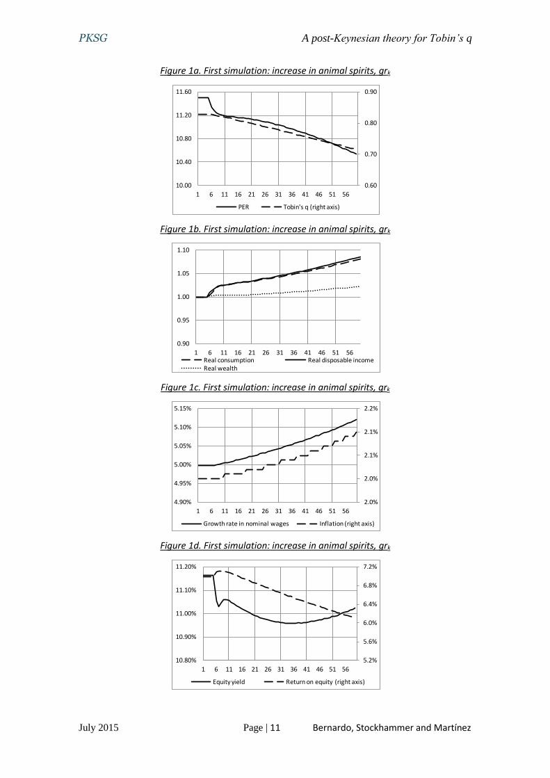
An increase in the growth rate of the economy
The first simulation will deal with an increase in the growth rate of the capital stock, 𝑔𝑟𝑘,
which from a Keynesian point of view can be regarded as an increase in animal spirits. Figures
1 to 4 show the results. The first chart confirms the Kaldorian conclusion that higher growth
rates yield lower valuation ratios. However, not much attention should be placed in this case
to short-term results, given the way financial markets have been introduced in the picture,
because one should expect that financial markets should include higher growth rate
expectations into equity prices in the short-run – the empirical evidence suggests that markets
almost always overreact. In any case, the secular decline in the long-run can be explained by
the increase in the inflation rate, which affects not only financial market indicators but
corporations’ return on equity as well, through higher values of capital at replacement cost.
This result is in contrast to the Cambridge model, where higher growth rates lead to higher
profit rates. Here, although economic activity improves (both in the short-run and in the long-
run), the fact that the return on equity is measured with capital in nominal values (as it should)
leads to a decline of the return on equity over time.
PKSG A post-Keynesian theory for Tobin’s q
July 2015 Page | 11 Bernardo, Stockhammer and Martínez
Figure 1a. First simulation: increase in animal spirits, grk
Figure 1b. First simulation: increase in animal spirits, grk
Figure 1c. First simulation: increase in animal spirits, grk
Figure 1d. First simulation: increase in animal spirits, grk
0.60
0.70
0.80
0.90
10.00
10.40
10.80
11.20
11.60
1 6 11 16 21 26 31 36 41 46 51 56
PER Tobin's q (right axis)
0.90
0.95
1.00
1.05
1.10
1 6 11 16 21 26 31 36 41 46 51 56Real consumption Real disposable incomeReal wealth
2.0%
2.0%
2.1%
2.1%
2.2%
4.90%
4.95%
5.00%
5.05%
5.10%
5.15%
1 6 11 16 21 26 31 36 41 46 51 56
Growth rate in nominal wages Inflation (right axis)
5.2%
5.6%
6.0%
6.4%
6.8%
7.2%
10.80%
10.90%
11.00%
11.10%
11.20%
1 6 11 16 21 26 31 36 41 46 51 56
Equity yield Return on equity (right axis)
PKSG A post-Keynesian theory for Tobin’s q
July 2015 Page | 12 Bernardo, Stockhammer and Martínez
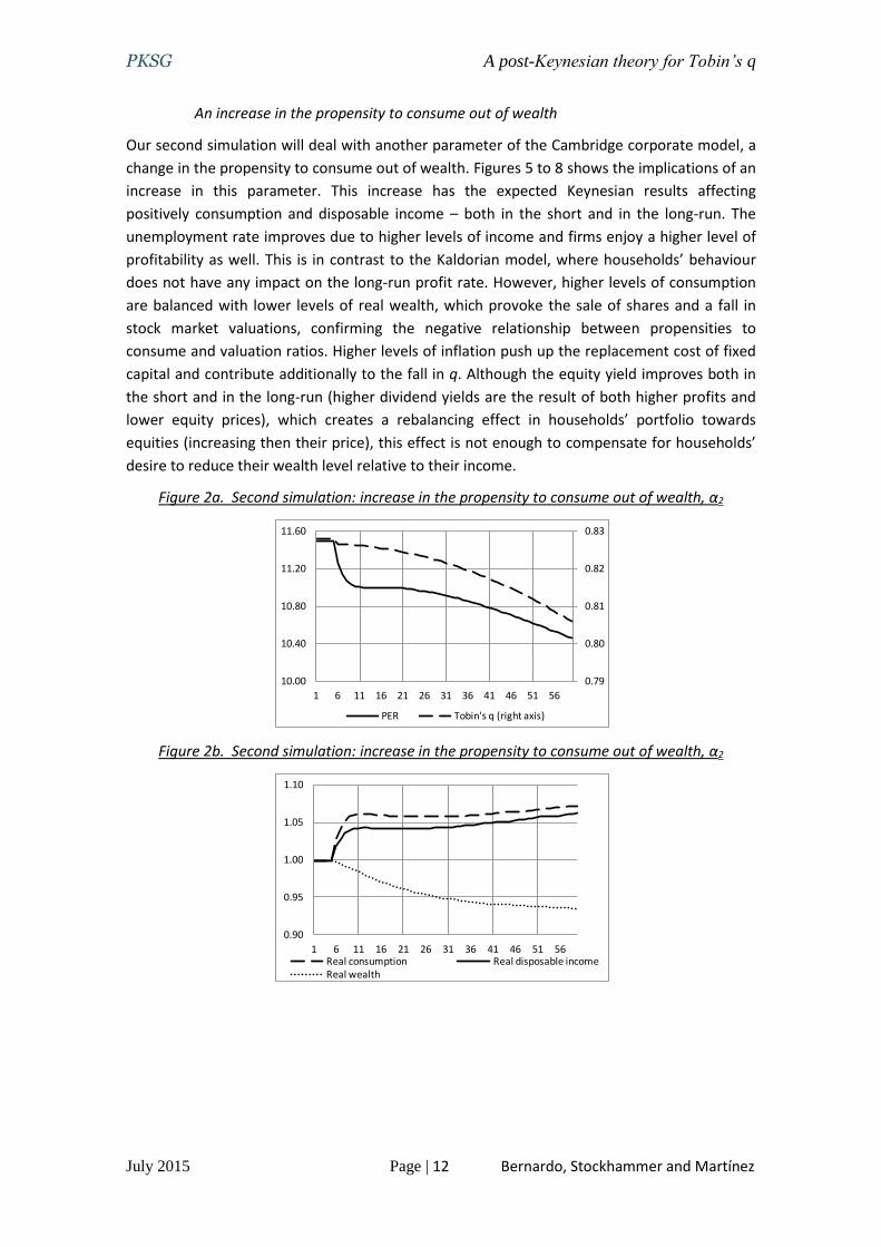
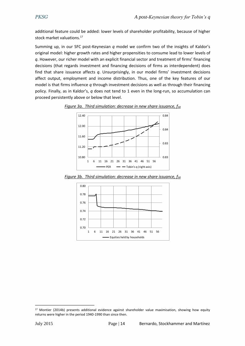
An increase in the propensity to consume out of wealth
Our second simulation will deal with another parameter of the Cambridge corporate model, a
change in the propensity to consume out of wealth. Figures 5 to 8 shows the implications of an
increase in this parameter. This increase has the expected Keynesian results affecting
positively consumption and disposable income – both in the short and in the long-run. The
unemployment rate improves due to higher levels of income and firms enjoy a higher level of
profitability as well. This is in contrast to the Kaldorian model, where households’ behaviour
does not have any impact on the long-run profit rate. However, higher levels of consumption
are balanced with lower levels of real wealth, which provoke the sale of shares and a fall in
stock market valuations, confirming the negative relationship between propensities to
consume and valuation ratios. Higher levels of inflation push up the replacement cost of fixed
capital and contribute additionally to the fall in q. Although the equity yield improves both in
the short and in the long-run (higher dividend yields are the result of both higher profits and
lower equity prices), which creates a rebalancing effect in households’ portfolio towards
equities (increasing then their price), this effect is not enough to compensate for households’
desire to reduce their wealth level relative to their income.
Figure 2a. Second simulation: increase in the propensity to consume out of wealth, α2
Figure 2b. Second simulation: increase in the propensity to consume out of wealth, α2
0.79
0.80
0.81
0.82
0.83
10.00
10.40
10.80
11.20
11.60
1 6 11 16 21 26 31 36 41 46 51 56
PER Tobin's q (right axis)
0.90
0.95
1.00
1.05
1.10
1 6 11 16 21 26 31 36 41 46 51 56Real consumption Real disposable incomeReal wealth
PKSG A post-Keynesian theory for Tobin’s q
July 2015 Page | 13 Bernardo, Stockhammer and Martínez
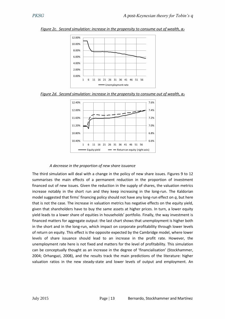
Figure 2c. Second simulation: increase in the propensity to consume out of wealth, α2
Figure 2d. Second simulation: increase in the propensity to consume out of wealth, α2
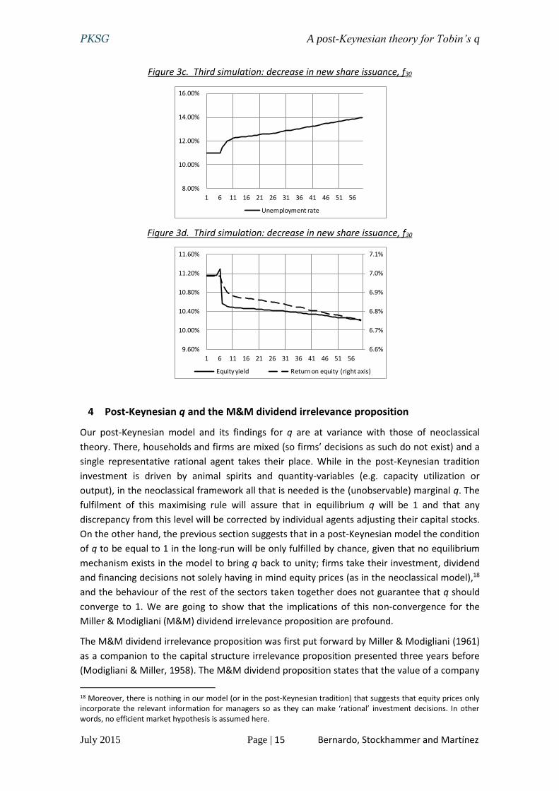
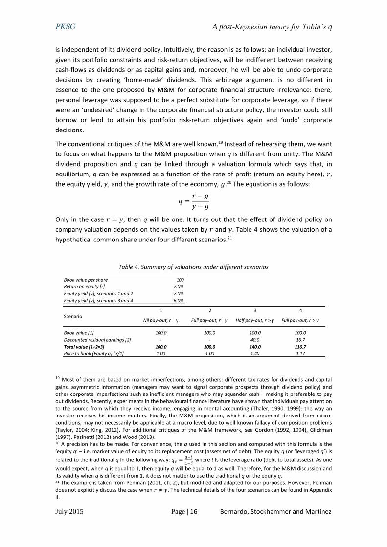
A decrease in the proportion of new share issuance
The third simulation will deal with a change in the policy of new share issues. Figures 9 to 12
summarises the main effects of a permanent reduction in the proportion of investment
financed out of new issues. Given the reduction in the supply of shares, the valuation metrics
increase notably in the short run and they keep increasing in the long-run. The Kaldorian
model suggested that firms’ financing policy should not have any long-run effect on q, but here
that is not the case. The increase in valuation metrics has negative effects on the equity yield,
given that shareholders have to buy the same assets at higher prices. In turn, a lower equity
yield leads to a lower share of equities in households’ portfolio. Finally, the way investment is
financed matters for aggregate output: the last chart shows that unemployment is higher both
in the short and in the long-run, which impact on corporate profitability through lower levels
of return on equity. This effect is the opposite expected by the Cambridge model, where lower
levels of share issuance should lead to an increase in the profit rate. However, the
unemployment rate here is not fixed and matters for the level of profitability. This simulation
can be conceptually thought as an increase in the degree of ‘financialisation’ (Stockhammer,
2004; Orhangazi, 2008), and the results track the main predictions of the literature: higher
valuation ratios in the new steady-state and lower levels of output and employment. An
0.00%
2.00%
4.00%
6.00%
8.00%
10.00%
12.00%
1 6 11 16 21 26 31 36 41 46 51 56
Unemployment rate
6.6%
6.8%
7.0%
7.2%
7.4%
7.6%
10.40%
10.80%
11.20%
11.60%
12.00%
12.40%
1 6 11 16 21 26 31 36 41 46 51 56
Equity yield Return on equity (right axis)
PKSG A post-Keynesian theory for Tobin’s q
July 2015 Page | 14 Bernardo, Stockhammer and Martínez
additional feature could be added: lower levels of shareholder profitability, because of higher
stock market valuations.17
Summing up, in our SFC post-Keynesian q model we confirm two of the insights of Kaldor’s
original model: higher growth rates and higher propensities to consume lead to lower levels of
q. However, our richer model with an explicit financial sector and treatment of firms’ financing
decisions (that regards investment and financing decisions of firms as interdependent) does
find that share issuance affects q. Unsurprisingly, in our model firms’ investment decisions
affect output, employment and income distribution. Thus, one of the key features of our
model is that firms influence q through investment decisions as well as through their financing
policy. Finally, as in Kaldor’s, q does not tend to 1 even in the long-run, so accumulation can
proceed persistently above or below that level.
Figure 3a. Third simulation: decrease in new share issuance, f30
Figure 3b. Third simulation: decrease in new share issuance, f30
17 Montier (2014b) presents additional evidence against shareholder value maximisation, showing how equity returns were higher in the period 1940-1990 than since then.
0.83
0.83
0.84
0.84
10.80
11.20
11.60
12.00
12.40
1 6 11 16 21 26 31 36 41 46 51 56
PER Tobin's q (right axis)
0.70
0.72
0.74
0.76
0.78
0.80
1 6 11 16 21 26 31 36 41 46 51 56
Equities held by households
PKSG A post-Keynesian theory for Tobin’s q
July 2015 Page | 15 Bernardo, Stockhammer and Martínez
Figure 3c. Third simulation: decrease in new share issuance, f30
Figure 3d. Third simulation: decrease in new share issuance, f30
4 Post-Keynesian q and the M&M dividend irrelevance proposition
Our post-Keynesian model and its findings for q are at variance with those of neoclassical
theory. There, households and firms are mixed (so firms’ decisions as such do not exist) and a
single representative rational agent takes their place. While in the post-Keynesian tradition
investment is driven by animal spirits and quantity-variables (e.g. capacity utilization or
output), in the neoclassical framework all that is needed is the (unobservable) marginal q. The
fulfilment of this maximising rule will assure that in equilibrium q will be 1 and that any
discrepancy from this level will be corrected by individual agents adjusting their capital stocks.
On the other hand, the previous section suggests that in a post-Keynesian model the condition
of q to be equal to 1 in the long-run will be only fulfilled by chance, given that no equilibrium
mechanism exists in the model to bring q back to unity; firms take their investment, dividend
and financing decisions not solely having in mind equity prices (as in the neoclassical model),18
and the behaviour of the rest of the sectors taken together does not guarantee that q should
converge to 1. We are going to show that the implications of this non-convergence for the
Miller & Modigliani (M&M) dividend irrelevance proposition are profound.
The M&M dividend irrelevance proposition was first put forward by Miller & Modigliani (1961)
as a companion to the capital structure irrelevance proposition presented three years before
(Modigliani & Miller, 1958). The M&M dividend proposition states that the value of a company
18 Moreover, there is nothing in our model (or in the post-Keynesian tradition) that suggests that equity prices only incorporate the relevant information for managers so as they can make ‘rational’ investment decisions. In other words, no efficient market hypothesis is assumed here.
8.00%
10.00%
12.00%
14.00%
16.00%
1 6 11 16 21 26 31 36 41 46 51 56
Unemployment rate
6.6%
6.7%
6.8%
6.9%
7.0%
7.1%
9.60%
10.00%
10.40%
10.80%
11.20%
11.60%
1 6 11 16 21 26 31 36 41 46 51 56
Equity yield Return on equity (right axis)
PKSG A post-Keynesian theory for Tobin’s q
July 2015 Page | 16 Bernardo, Stockhammer and Martínez
is independent of its dividend policy. Intuitively, the reason is as follows: an individual investor,
given its portfolio constraints and risk-return objectives, will be indifferent between receiving
cash-flows as dividends or as capital gains and, moreover, he will be able to undo corporate
decisions by creating ‘home-made’ dividends. This arbitrage argument is no different in
essence to the one proposed by M&M for corporate financial structure irrelevance: there,
personal leverage was supposed to be a perfect substitute for corporate leverage, so if there
were an ‘undesired’ change in the corporate financial structure policy, the investor could still
borrow or lend to attain his portfolio risk-return objectives again and ‘undo’ corporate
decisions.
The conventional critiques of the M&M are well known.19 Instead of rehearsing them, we want
to focus on what happens to the M&M proposition when q is different from unity. The M&M
dividend proposition and q can be linked through a valuation formula which says that, in
equilibrium, q can be expressed as a function of the rate of profit (return on equity here), 𝑟,
the equity yield, 𝛾, and the growth rate of the economy, 𝑔.20 The equation is as follows:
𝑞 =𝑟 − 𝑔
𝑦 − 𝑔
Only in the case 𝑟 = 𝑦, then q will be one. It turns out that the effect of dividend policy on
company valuation depends on the values taken by 𝑟 and 𝑦. Table 4 shows the valuation of a
hypothetical common share under four different scenarios.21
Table 4. Summary of valuations under different scenarios
19 Most of them are based on market imperfections, among others: different tax rates for dividends and capital
gains, asymmetric information (managers may want to signal corporate prospects through dividend policy) and other corporate imperfections such as inefficient managers who may squander cash – making it preferable to pay out dividends. Recently, experiments in the behavioural finance literature have shown that individuals pay attention to the source from which they receive income, engaging in mental accounting (Thaler, 1990, 1999): the way an investor receives his income matters. Finally, the M&M proposition, which is an argument derived from micro-conditions, may not necessarily be applicable at a macro level, due to well-known fallacy of composition problems (Taylor, 2004; King, 2012). For additional critiques of the M&M framework, see Gordon (1992, 1994), Glickman (1997), Pasinetti (2012) and Wood (2013). 20 A precision has to be made. For convenience, the q used in this section and computed with this formula is the ‘equity q’ – i.e. market value of equity to its replacement cost (assets net of debt). The equity q (or ‘leveraged q’) is
related to the traditional q in the following way: 𝑞𝑒 =𝑞−𝑙
1−𝑙, where 𝑙 is the leverage ratio (debt to total assets). As one
would expect, when q is equal to 1, then equity q will be equal to 1 as well. Therefore, for the M&M discussion and its validity when q is different from 1, it does not matter to use the traditional q or the equity q. 21 The example is taken from Penman (2011, ch. 2), but modified and adapted for our purposes. However, Penman does not explicitly discuss the case when 𝑟 ≠ 𝛾. The technical details of the four scenarios can be found in Appendix II.
Book value per share 100
Return on equity [r] 7.0%
Equity yield [γ], scenarios 1 and 2 7.0%
Equity yield [γ], scenarios 3 and 4 6.0%
1 2 3 4
Nil pay-out, r = γ Full pay-out, r = γ Half pay-out, r > γ Full pay-out, r > γ
Book value [1] 100.0 100.0 100.0 100.0
Discounted residual earnings [2] - - 40.0 16.7
Total value [1+2=3] 100.0 100.0 140.0 116.7
Price to book (Equity q) [3/1] 1.00 1.00 1.40 1.17
Scenario
PKSG A post-Keynesian theory for Tobin’s q
July 2015 Page | 17 Bernardo, Stockhammer and Martínez
Table 4 shows that dividend policy is irrelevant only when the rate of profit (return on equity)
is equal to the equity yield or, in other words, when q is equal to 1: in this case, the pay-out
ratio chosen by the firm does not matter, because the value of the enterprise will remain
constant. However, this is not the case when the previous equality does not hold and q is
different from 1: changes in pay-out ratios will affect the value of the company,22 because the
difference between 𝑟 and 𝛾 makes that dividends and capital gains are not any longer in the
same footing. In the first two scenarios, the value remains the same because it is financially
equivalent to receive dividends and reinvest them at the market rate than to accumulate
unrealised capital gains (through higher equity prices) because of higher retained profits.
However, in the other two cases, the rate of return is higher than the equity yield, so the
investor is better off if the company decides to reinvest the earnings rather than to distribute
them as dividends – i.e. the investor would obtain a lower reinvestment rate in the market in
the latter case.
Therefore, from an empirical standpoint, as long as q is not equal to unity the M&M dividend
irrelevance proposition will not hold, because dividends and unrealised capital gains cannot be
treated as financially alike. An empirical analysis of q is beyond the scope of this paper, but
suffice it to say that the historical evidence in the developed countries since 1950 shows that q
has been persistently different from 1 – and trending up or down for whole decades. This is
crucial empirical evidence for the relevance of corporations’ dividend decisions on equity
valuations.
5 Conclusions
The present essay has proposed a post-Keynesian q theory at the macroeconomic level based
on Kaldor’s (1966) seminal paper. The Kaldorian model provides two important
macroeconomic long-run relationships, between q and the growth rate of the economy and q
and propensities to consume. We claim that these relationships alone can provide new
valuable insights on long-run relationships between financial (equity) markets and
macroeconomics. Our medium-scale SFC post-Keynesian model has improved the simplistic
monetary and financial framework of the Kaldorian model and has shown that in this enriched
setup these two long-run relationships still hold. Our model has also addressed, following
Gordon (1992), the interdependence between firms’ financing decisions and dividend policy,
and aspect often overlooked but crucial for the understanding of financial markets. On the
other hand, our model does find that share issuance (and more generally, firms’ financing
decisions) affects q, whereas in the Kaldorian model q was independent of firms’ financing
policy. Furthermore, the Kaldorian insight that, in general, q will be different from 1 in the long
run, is confirmed by the numerical simulations. Independent sectors with different motivations
make possible that accumulation can proceed with q levels different from unity.
Finally, this non-convergence impinges on the validity of the Miller-Modigliani dividend
irrelevance proposition. As long as q is different from 1, the proposition does not hold,
because in this case capital gains and dividends cannot be considered financially equivalent, so
firms’ dividend policy will affect equity valuation. The empirical evidence is against the M&M
proposition. Economic theory should consider a q different from 1 as part of the financial
22 For brevity’s sake, only the case when 𝑟 > 𝛾 is considered here.
PKSG A post-Keynesian theory for Tobin’s q
July 2015 Page | 18 Bernardo, Stockhammer and Martínez
markets stylized facts. Post-Keynesian macroeconomic theory can explain this, even in the
absence of speculation or other persistent behavioural biases.
References
Abel, A., & Blanchard, O. (1986). The Present Value of Profits and Cyclical Movements in
Investment. Econometrica, 54(2), 249–273.
Araujo, J. T. (1995). Kaldor’s Neo-Pasinetti Theorem and the Cambridge Theory of Distribution.
Manchester School of Social and Economic Studies, September, 311–317.
Baranzini, M., & Mirante, A. (2013). The Cambridge Post-Keynesian School of Income and
Wealth Distribution. In G. C. Harcourt & P. Kriesler (Eds.), The Oxford Handbook of Post-
Keynesian Economics. Volume 1: Theory and Origins (pp. 288–361). Oxford: Oxford
University Press.
Blundell, R., Bond, S., Devereux, M., & Schiantarelli, F. (1992). Investment and Tobin’s Q:
Evidence from Company Panel Data. Journal of Econometrics, 51, 233–257.
Brainard, W., & Tobin, J. (1968). Pitfalls in Financial Model Building. American Economic
Review, 58(2), 99–122.
Carlin, W., & Soskice, D. W. (2006). Macroeconomics: Imperfections, Institutions, and Policies.
Oxford University Press.
Chirinko, R. (1993). Business Fixed Investment Spending: Modeling Strategies, Empirical
Results, and Policy Implications. Journal of Economic Literature, 31(4), 1875–1991.
Christiano, L., Eichenbaum, M., & Evans, C. (2005). Nominal Rigidities and the Dynamic Effects
of a Shock to Monetary Policy. Journal of Political Economy, 113(1), 1–45.
Cohen, A., & Harcourt, G. C. (2003). Whatever Happened to the Cambridge Capital Theory
Controversies. Journal of Economic Perspectives, 17(1), 199–214.
Commendatore, P. (2003). On the Post Keynesian Theory of Growth and “Institutional”
Distribution. Review of Political Economy, 15(2), 193–209.
Crotty, J. (1990). Owner-Manager Conflict and Financial Theories of Investment Instability: A
Critical Assessment of Keynes, Tobin and Minsky. Journal of Post Keynesian Economics,
12(4), 519–542.
Dalziel, P. (1991). A Generalisation and Simplification of the Cambridge Theorem with Budget
Deficits. Cambridge Journal of Economics, 15, 287–300.
Davidson, P. (1968). The Demand and Supply of Securities and Economic Growth and its
Implications for the Kaldor-Pasinetti Versus Samuelson-Modigliani Controversy. The
American Economic Review, 58(2), 252–269.
Dos Santos, C. H., & Zezza, G. (2008). A Simplified, “Benchmark”, Stock-Flow Consistent Post-
Keynesian Growth Model. Metroeconomica, 59(3), 441–478.
PKSG A post-Keynesian theory for Tobin’s q
July 2015 Page | 19 Bernardo, Stockhammer and Martínez
Felipe, J., & Fisher, F. (2003). Aggregation in Production Functions: What Applied Economists
Should Know. Metroeconomica, 54(2), 208–262.
Felipe, J., & McCombie, J. (2013). The Aggregate Production Function and the Measurement of
Technical Change: Not Even Wrong. Cheltenham, UK: Edward Elgar.
Fischer, S., & Merton, R. (1984). Macroeconomics and Finance: The Role of the Stock Market.
NBER Working Paper Series, 1291.
Glickman, M. (1997). A Post-Keynesian Refutation of Modigliani-Miller Capital Structure.
Journal of Post Keynesian Economics, 20(251-274).
Godley, W., & Lavoie, M. (2007). Monetary Economics (1st ed.). Basingstoke: Palgrave
MacMillan.
Gordon, M. J. (1963). Optimal Investment and Financing Policy. The Journal of Finance, 18(2),
264–272.
Gordon, M. J. (1992). The Neoclassical and a Post Keynesian Theory of Investment. Journal of
Post Keynesian Economics, 14(4), 425–443.
Gordon, M. J. (1994). Finance, Investment, and Macroeconomics: The Neoclassical and a Post
Keynesian Solution. Cheltenham: Edward Elgar.
Gordon, M. J., & Shapiro, E. (1956). Capital Equipment Analysis: The Required Rate of Profit.
Management Science, 3(1), 102–110.
Hayashi, F. (1982). Tobin’s Marginal q and Average q: A Neoclassical Interpretation.
Econometrica, 50(1), 213–224.
Hein, E., Lavoie, M., & Van Treeck, T. (2011). Some Instability Puzzles in Kaleckian Models of
Growth and Distribution: A Critical Survey. Cambridge Journal of Economics, 35(3), 587–
612.
Hein, E., Lavoie, M., & Van Treeck, T. (2012). Harrodian Instability and the “Normal Rate” of
Capacity Utilisation in Kaleckian Models of Distribution and Growth - A Survey.
Metroeconomica, 63(1), 139–169.
Jefferson, T., & King, J. (2010). Can Post Keynesians Make Better Use of Behavioral Economics?
Journal of Post Keynesian Economics, 33(2), 211–234.
Kaldor, N. (1955). Alternative Theories of Distribution. The Review of Economic Studies, 23(2),
83–100.
Kaldor, N. (1966). Marginal Productivity and the Macro-Economic Theories of Distribution.
Review of Economic Studies, 33, 309–319.
Keynes, J. M. (1936). The General Theory of Employment, Interest and Money. London:
Macmillan Press.
King, J. (2012). The Microfoundations Delusion. Metaphor and Dogma in the History of
Macroeconomics. Cheltenham, UK: Edward Elgar.
PKSG A post-Keynesian theory for Tobin’s q
July 2015 Page | 20 Bernardo, Stockhammer and Martínez
Kregel, J. (1985). Hamlet without the Prince: Cambridge Macroeconomics without Money. The
American Economic Review, 75(2), 133–139.
Lavoie, M. (1998). The Neo-Pasinetti Theorem in Cambridgian and Kaleckian Models of Growth
and Distribution. Eastern Economic Journal, 24(4), 417–434.
Lavoie, M. (2014). Post-Keynesian Economics: New Foundations. Cheltenham, UK: Edward
Elgar.
Lavoie, M., & Godley, W. (2001). Kaleckian Models of Growth in a Coherent Stock-Flow
Monetary Framework: a Kaldorian View. Journal of Post Keynesian Economics, 24(2),
277–311.
Le Heron, E., & Mouakil, T. (2008). A Post-Keynesian Stock-Flow Consistent Model for Dynamic
Analysis of Monetary Policy Shock on Banking Behaviour. Metroeconomica, 59(3), 405–
440.
Lintner, J. (1962). Dividends, Earnings, Leverage, Stock Prices and the Supply of Capital to
Corporations. The Review of Economics and Statistics, 44(3), 243–269.
Lucas, R., & Prescott, E. (1971). Investment Under Uncertainty. Econometrica, 39(5), 659–681.
Marris, R. (1972). Why Economics Needs a Theory of the Firm. Economic Journal, 82, 321–352.
Miller, M. H., & Modigliani, F. (1961). Dividend Policy, Growth, and the Valuation of Shares.
The Journal of Business, 34(4), 411–433.
Minsky, H. P. (2008). John Maynard Keynes (2nd ed.). New York: McGraw-Hill.
Modigliani, F., & Miller, M. H. (1958). The Cost of Capital, Corporation Finance and the Theory
of Investment. The American Economic Review, 48(3), 261–297.
Montier, J. (2014a). A Cape Crusader - A Defence Against the Dark Arts. GMO - White Paper,
February.
Montier, J. (2014b). The World’s Dumbest Idea. GMO - White Paper, (December).
Moore, B. (1973). Some Macroeconomic Consequences of Corporate Equities. Canadian
Journal of Economics, November, 529–544.
Moore, B. (1975). Equities, Capital Gains, and the Role of Finance in Accumulation. American
Economic Review, December, 872–886.
Moss, S. J. (1978). The Post-Keynesian Theory of Income Distribution in the Corporate
Economy. Australian Economic Papers, (December), 303–322.
Orhangazi, Ö. (2008). Financialisation and Capital Accumulation in the Non-Financial Corporate
Sector: A Theoretical and Empirical Investigation on the US Economy: 1973-2003.
Cambridge Journal of Economics, 32(6), 863–886.
Palley, T. (1996). Inside Debt, Aggregate Demand, and the Cambridge Theory of Distribution.
Cambridge Journal of Economics, 20(4), 465–474.
Palley, T. (2001). The Stock Market and Investment: Another Look at the Micro-Foundations of
q Theory. Cambridge Journal of Economics, 25, 657–667.
PKSG A post-Keynesian theory for Tobin’s q
July 2015 Page | 21 Bernardo, Stockhammer and Martínez
Panico, C. (1997). Government Deficits in post-Keynesian Theories of Growth and Distribution.
Contributions to Political Economy, 16(1), 61–86.
Park, M.-S. (2006). The Financial System and the Pasinetti Theorem. Cambridge Journal of
Economics, 30(2), 201–217.
Pasinetti, L. L. (1962). Rate of Profit and Income Distribution in Relation to the Rate of
Economic Growth. The Review of Economic Studies, 29(4), 267–279.
Pasinetti, L. L. (1989). Ricardian Debt/Taxation Equivalence in the Kaldor Theory of Profits and
Income Distribution. Cambridge Journal of Economics, 13(1), 25–36.
Pasinetti, L. L. (2012). A Few Counter-Factual Hypotheses on the Current Economic Crisis.
Cambridge Journal of Economics, 36(6), 1433–1453.
Penman, S. (2011). Accounting for Value. New York: Columbia University Press.
Piketty, T. (2014). Capital in the Twenty-First Century. Cambridge, Massachusetts: Belknap
Press, Harvard University Press.
Robinson, J. (1956). The Accumulation of Capital. London: Blackwell.
Romer, D. (2012). Advanced Macroeconomics (4th ed.). New York: McGraw-Hill.
Samuelson, P., & Modigliani, F. (1966). The Pasinetti Paradox in Neoclassical and More General
Models. Review of Economic Studies, 33(4), 269–301.
Smets, F., & Wouters, R. (2007). Shocks and Frictions in US Business Cycles: A Bayesian DSGE
Approach. The American Economic Review, 97(3), 586–606.
Smithers, A. (2009). Wall Street Revalued. Imperfect Markets and Inept Central Bankers.
Chichester: Wiley & Sons.
Steedman, I. (1972). The State and the Outcome of the Pasinetti Process. Economic Journal,
82(December), 1387–1395.
Stockhammer, E. (2004). Financialisation and the Slowdown of Accumulation. Cambridge
Journal of Economics, 28(5), 719–741.
Summers, L. H. (1981). Taxation and Corporate Investment: A q-Theory Approach. Brookings
Papers on Economic Activity, 1981(1), 67–127.
Taylor, L. (2004). Reconstructing Macroeconomics. Cambridge, Massachusetts: Harvard
University Press.
Thaler, R. (1990). Anomalies: Saving, Fungibility and Mental Accounts. Journal of Economic
Perspectives, 4(1), 193–205.
Thaler, R. (1999). Mental Accounting Matters. Journal of Behavioral Decision Making, 12, 183–
206.
Thaler, R. H. (Ed.). (2005). Advances in Behavioral Finance (Volume II). New Jersey: Princeton
University Press.
PKSG A post-Keynesian theory for Tobin’s q
July 2015 Page | 22 Bernardo, Stockhammer and Martínez
Tobin, J. (1969). A General Equilibrium Approach to Monetary Theory. Journal of Money,
Credit, and Banking, 1(1), 15–29.
Tobin, J. (1984). On the Efficiency of the Financial System. Lloyds Bank Review, (July), 1–15.
Tobin, J., & Brainard, W. (1977). Asset Markets and the Cost of Capital. In B. Balassa & R.
Nelson (Eds.), Economic Progress, Private Values, and Public Policy: Essays in Honor of
William Fellner (pp. 235–262). New York: North Holland.
Tobin, J., & Brainard, W. (1990). On Crotty’s Critique of q-Theory. Journal of Post Keynesian
Economics, 12(4), 543–549.
Van Treeck, T. (2008). A Synthetic, Stock-Flow Consistent Macroeconomic Model of
“Financialisation.” Cambridge Journal of Economics, 33(3), 467–493.
Walter, J. E. (1963). Dividend Policy: Its Influence on the Value of the Enterprise. The Journal of
Finance, 18(2), 280–291.
Woods, J. E. (2013). Note: Pasinetti’s Counter-Factual Hypotheses. Cambridge Journal of
Economics, 37(6), 1431–1435.
Yoshikawa, H. (1980). On the “q” Theory of Investment. The American Economic Review, 70(4),
739–743.
Zezza, G. (2008). U.S. Growth, the Housing Market, and the Distribution of Income. Journal of
Post Keynesian Economics, 30(3), 375–401.
Appendix I. List of equations of the model, values used in the simulations and
matrices of the model
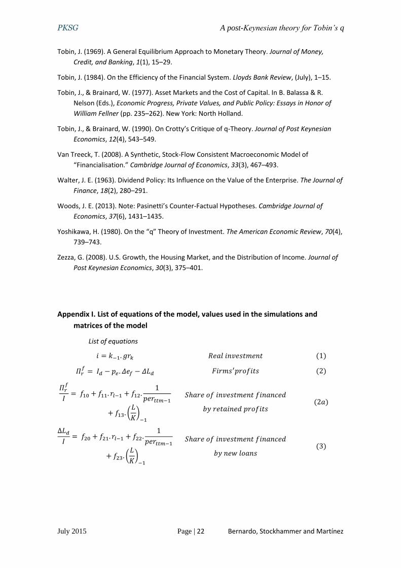
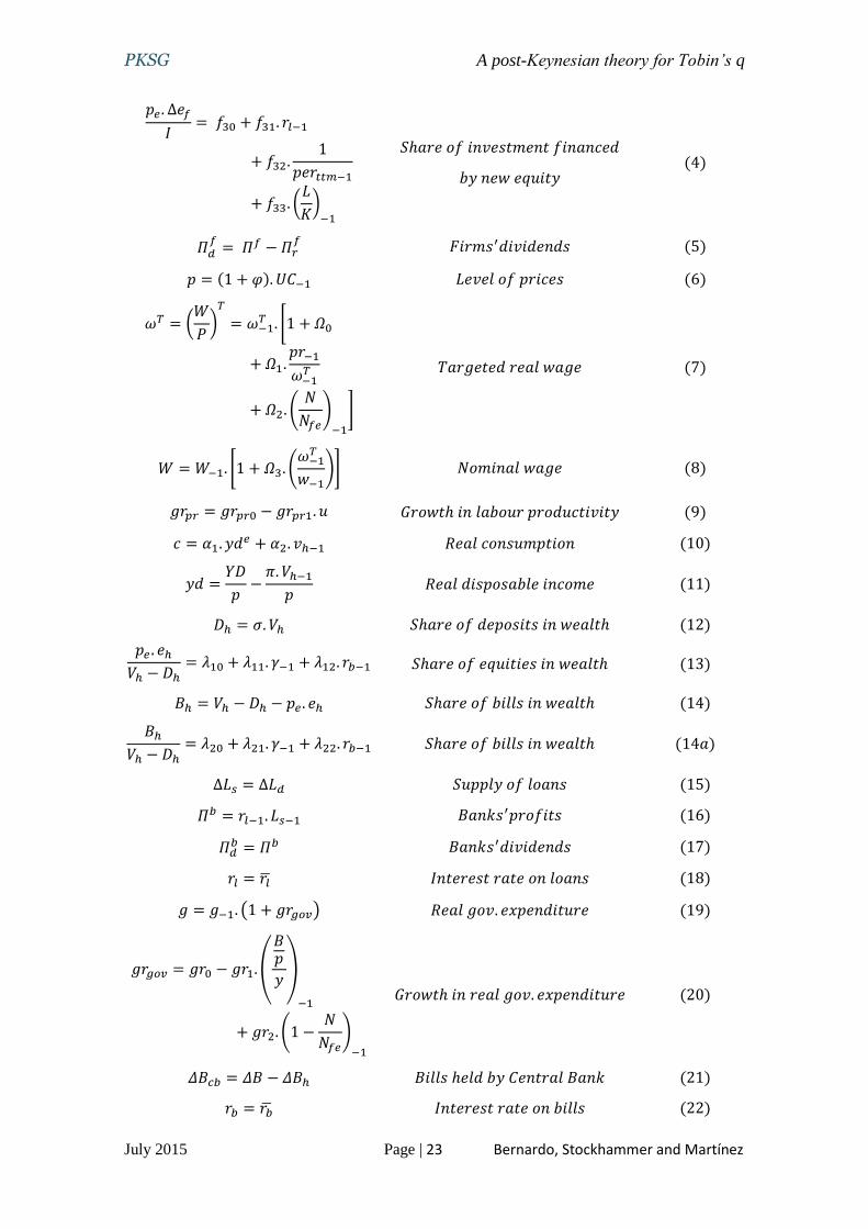
List of equations
𝑖 = 𝑘−1. 𝑔𝑟𝑘 𝑅𝑒𝑎𝑙 𝑖𝑛𝑣𝑒𝑠𝑡𝑚𝑒𝑛𝑡 (1)
𝛱𝑟𝑓
= 𝐼𝑑 − 𝑝𝑒 . 𝛥𝑒𝑓 − 𝛥𝐿𝑑 𝐹𝑖𝑟𝑚𝑠′𝑝𝑟𝑜𝑓𝑖𝑡𝑠 (2)
𝛱𝑟𝑓
𝐼= 𝑓10 + 𝑓11. 𝑟𝑙−1 + 𝑓12.
1
𝑝𝑒𝑟𝑡𝑡𝑚−1
+ 𝑓13. (𝐿
𝐾)
−1
𝑆ℎ𝑎𝑟𝑒 𝑜𝑓 𝑖𝑛𝑣𝑒𝑠𝑡𝑚𝑒𝑛𝑡 𝑓𝑖𝑛𝑎𝑛𝑐𝑒𝑑
𝑏𝑦 𝑟𝑒𝑡𝑎𝑖𝑛𝑒𝑑 𝑝𝑟𝑜𝑓𝑖𝑡𝑠 (2𝑎)
∆𝐿𝑑
𝐼= 𝑓20 + 𝑓21. 𝑟𝑙−1 + 𝑓22.
1
𝑝𝑒𝑟𝑡𝑡𝑚−1
+ 𝑓23. (𝐿
𝐾)
−1
𝑆ℎ𝑎𝑟𝑒 𝑜𝑓 𝑖𝑛𝑣𝑒𝑠𝑡𝑚𝑒𝑛𝑡 𝑓𝑖𝑛𝑎𝑛𝑐𝑒𝑑
𝑏𝑦 𝑛𝑒𝑤 𝑙𝑜𝑎𝑛𝑠 (3)
PKSG A post-Keynesian theory for Tobin’s q
July 2015 Page | 23 Bernardo, Stockhammer and Martínez
𝑝𝑒 . ∆𝑒𝑓
𝐼= 𝑓30 + 𝑓31. 𝑟𝑙−1
+ 𝑓32.1
𝑝𝑒𝑟𝑡𝑡𝑚−1
+ 𝑓33. (𝐿
𝐾)
−1
𝑆ℎ𝑎𝑟𝑒 𝑜𝑓 𝑖𝑛𝑣𝑒𝑠𝑡𝑚𝑒𝑛𝑡 𝑓𝑖𝑛𝑎𝑛𝑐𝑒𝑑
𝑏𝑦 𝑛𝑒𝑤 𝑒𝑞𝑢𝑖𝑡𝑦 (4)
𝛱𝑑𝑓
= 𝛱𝑓 − 𝛱𝑟𝑓 𝐹𝑖𝑟𝑚𝑠′𝑑𝑖𝑣𝑖𝑑𝑒𝑛𝑑𝑠 (5)
𝑝 = (1 + 𝜑). 𝑈𝐶−1 𝐿𝑒𝑣𝑒𝑙 𝑜𝑓 𝑝𝑟𝑖𝑐𝑒𝑠 (6)
𝜔𝑇 = (𝑊
𝑃)
𝑇
= 𝜔−1𝑇 . [1 + 𝛺0
+ 𝛺1.𝑝𝑟−1
𝜔−1𝑇
+ 𝛺2. (𝑁
𝑁𝑓𝑒)
−1
]
𝑇𝑎𝑟𝑔𝑒𝑡𝑒𝑑 𝑟𝑒𝑎𝑙 𝑤𝑎𝑔𝑒 (7)
𝑊 = 𝑊−1. [1 + 𝛺3. (𝜔−1
𝑇
𝑤−1)] 𝑁𝑜𝑚𝑖𝑛𝑎𝑙 𝑤𝑎𝑔𝑒 (8)
𝑔𝑟𝑝𝑟 = 𝑔𝑟𝑝𝑟0 − 𝑔𝑟𝑝𝑟1. 𝑢 𝐺𝑟𝑜𝑤𝑡ℎ 𝑖𝑛 𝑙𝑎𝑏𝑜𝑢𝑟 𝑝𝑟𝑜𝑑𝑢𝑐𝑡𝑖𝑣𝑖𝑡𝑦 (9)
𝑐 = 𝛼1. 𝑦𝑑𝑒 + 𝛼2. 𝑣ℎ−1 𝑅𝑒𝑎𝑙 𝑐𝑜𝑛𝑠𝑢𝑚𝑝𝑡𝑖𝑜𝑛 (10)
𝑦𝑑 =𝑌𝐷
𝑝−
𝜋. 𝑉ℎ−1
𝑝 𝑅𝑒𝑎𝑙 𝑑𝑖𝑠𝑝𝑜𝑠𝑎𝑏𝑙𝑒 𝑖𝑛𝑐𝑜𝑚𝑒 (11)
𝐷ℎ = 𝜎. 𝑉ℎ 𝑆ℎ𝑎𝑟𝑒 𝑜𝑓 𝑑𝑒𝑝𝑜𝑠𝑖𝑡𝑠 𝑖𝑛 𝑤𝑒𝑎𝑙𝑡ℎ (12)
𝑝𝑒 . 𝑒ℎ
𝑉ℎ − 𝐷ℎ= 𝜆10 + 𝜆11. 𝛾−1 + 𝜆12. 𝑟𝑏−1 𝑆ℎ𝑎𝑟𝑒 𝑜𝑓 𝑒𝑞𝑢𝑖𝑡𝑖𝑒𝑠 𝑖𝑛 𝑤𝑒𝑎𝑙𝑡ℎ (13)
𝐵ℎ = 𝑉ℎ − 𝐷ℎ − 𝑝𝑒 . 𝑒ℎ 𝑆ℎ𝑎𝑟𝑒 𝑜𝑓 𝑏𝑖𝑙𝑙𝑠 𝑖𝑛 𝑤𝑒𝑎𝑙𝑡ℎ (14)
𝐵ℎ
𝑉ℎ − 𝐷ℎ= 𝜆20 + 𝜆21. 𝛾−1 + 𝜆22. 𝑟𝑏−1 𝑆ℎ𝑎𝑟𝑒 𝑜𝑓 𝑏𝑖𝑙𝑙𝑠 𝑖𝑛 𝑤𝑒𝑎𝑙𝑡ℎ (14𝑎)
∆𝐿𝑠 = ∆𝐿𝑑 𝑆𝑢𝑝𝑝𝑙𝑦 𝑜𝑓 𝑙𝑜𝑎𝑛𝑠 (15)
𝛱𝑏 = 𝑟𝑙−1. 𝐿𝑠−1 𝐵𝑎𝑛𝑘𝑠′𝑝𝑟𝑜𝑓𝑖𝑡𝑠 (16)
𝛱𝑑𝑏 = 𝛱𝑏 𝐵𝑎𝑛𝑘𝑠′𝑑𝑖𝑣𝑖𝑑𝑒𝑛𝑑𝑠 (17)
𝑟𝑙 = 𝑟�̅� 𝐼𝑛𝑡𝑒𝑟𝑒𝑠𝑡 𝑟𝑎𝑡𝑒 𝑜𝑛 𝑙𝑜𝑎𝑛𝑠 (18)
𝑔 = 𝑔−1. (1 + 𝑔𝑟𝑔𝑜𝑣) 𝑅𝑒𝑎𝑙 𝑔𝑜𝑣. 𝑒𝑥𝑝𝑒𝑛𝑑𝑖𝑡𝑢𝑟𝑒 (19)
𝑔𝑟𝑔𝑜𝑣 = 𝑔𝑟0 − 𝑔𝑟1. (
𝐵𝑝
𝑦)
−1
+ 𝑔𝑟2. (1 −𝑁
𝑁𝑓𝑒)
−1
𝐺𝑟𝑜𝑤𝑡ℎ 𝑖𝑛 𝑟𝑒𝑎𝑙 𝑔𝑜𝑣. 𝑒𝑥𝑝𝑒𝑛𝑑𝑖𝑡𝑢𝑟𝑒 (20)
𝛥𝐵𝑐𝑏 = 𝛥𝐵 − 𝛥𝐵ℎ 𝐵𝑖𝑙𝑙𝑠 ℎ𝑒𝑙𝑑 𝑏𝑦 𝐶𝑒𝑛𝑡𝑟𝑎𝑙 𝐵𝑎𝑛𝑘 (21)
𝑟𝑏 = 𝑟�̅� 𝐼𝑛𝑡𝑒𝑟𝑒𝑠𝑡 𝑟𝑎𝑡𝑒 𝑜𝑛 𝑏𝑖𝑙𝑙𝑠 (22)
PKSG A post-Keynesian theory for Tobin’s q
July 2015 Page | 24 Bernardo, Stockhammer and Martínez
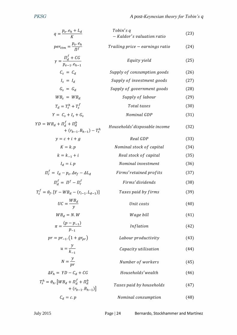
𝑞 =𝑝𝑒 . 𝑒ℎ + 𝐿𝑑
𝐾
𝑇𝑜𝑏𝑖𝑛′𝑠 𝑞
− 𝐾𝑎𝑙𝑑𝑜𝑟′𝑠 𝑣𝑎𝑙𝑢𝑎𝑡𝑖𝑜𝑛 𝑟𝑎𝑡𝑖𝑜 (23)
𝑝𝑒𝑟𝑡𝑡𝑚 =𝑝𝑒 . 𝑒ℎ
𝛱𝑓 𝑇𝑟𝑎𝑖𝑙𝑖𝑛𝑔 𝑝𝑟𝑖𝑐𝑒 − 𝑒𝑎𝑟𝑛𝑖𝑛𝑔𝑠 𝑟𝑎𝑡𝑖𝑜 (24)
𝛾 =𝛱𝑑
𝑓+ 𝐶𝐺
𝑝𝑒−1. 𝑒ℎ−1 𝐸𝑞𝑢𝑖𝑡𝑦 𝑦𝑖𝑒𝑙𝑑 (25)
𝐶𝑠 = 𝐶𝑑 𝑆𝑢𝑝𝑝𝑙𝑦 𝑜𝑓 𝑐𝑜𝑛𝑠𝑢𝑚𝑝𝑡𝑖𝑜𝑛 𝑔𝑜𝑜𝑑𝑠 (26)
𝐼𝑠 = 𝐼𝑑 𝑆𝑢𝑝𝑝𝑙𝑦 𝑜𝑓 𝑖𝑛𝑣𝑒𝑠𝑡𝑚𝑒𝑛𝑡 𝑔𝑜𝑜𝑑𝑠 (27)
𝐺𝑠 = 𝐺𝑑 𝑆𝑢𝑝𝑝𝑙𝑦 𝑜𝑓 𝑔𝑜𝑣𝑒𝑟𝑛𝑚𝑒𝑛𝑡 𝑔𝑜𝑜𝑑𝑠 (28)
𝑊𝐵𝑠 = 𝑊𝐵𝑑 𝑆𝑢𝑝𝑝𝑙𝑦 𝑜𝑓 𝑙𝑎𝑏𝑜𝑢𝑟 (29)
𝑇𝑑 = 𝑇𝑠ℎ + 𝑇𝑠
𝑓 𝑇𝑜𝑡𝑎𝑙 𝑡𝑎𝑥𝑒𝑠 (30)
𝑌 = 𝐶𝑠 + 𝐼𝑠 + 𝐺𝑠 𝑁𝑜𝑚𝑖𝑛𝑎𝑙 𝐺𝐷𝑃 (31)
𝑌𝐷 = 𝑊𝐵𝑑 + 𝛱𝑑𝑓
+ 𝛱𝑑𝑏
+ (𝑟𝑏−1. 𝐵ℎ−1) − 𝑇𝑠ℎ
𝐻𝑜𝑢𝑠𝑒ℎ𝑜𝑙𝑑𝑠′𝑑𝑖𝑠𝑝𝑜𝑠𝑎𝑏𝑙𝑒 𝑖𝑛𝑐𝑜𝑚𝑒 (32)
𝑦 = 𝑐 + 𝑖 + 𝑔 𝑅𝑒𝑎𝑙 𝐺𝐷𝑃 (33)
𝐾 = 𝑘. 𝑝 𝑁𝑜𝑚𝑖𝑛𝑎𝑙 𝑠𝑡𝑜𝑐𝑘 𝑜𝑓 𝑐𝑎𝑝𝑖𝑡𝑎𝑙 (34)
𝑘 = 𝑘−1 + 𝑖 𝑅𝑒𝑎𝑙 𝑠𝑡𝑜𝑐𝑘 𝑜𝑓 𝑐𝑎𝑝𝑖𝑡𝑎𝑙 (35)
𝐼𝑑 = 𝑖. 𝑝 𝑁𝑜𝑚𝑖𝑛𝑎𝑙 𝑖𝑛𝑣𝑒𝑠𝑡𝑚𝑒𝑛𝑡 (36)
𝛱𝑟𝑓
= 𝐼𝑑 − 𝑝𝑒 . 𝛥𝑒𝑓 − 𝛥𝐿𝑑 𝐹𝑖𝑟𝑚𝑠′𝑟𝑒𝑡𝑎𝑖𝑛𝑒𝑑 𝑝𝑟𝑜𝑓𝑖𝑡𝑠 (37)
𝛱𝑑𝑓
= 𝛱𝑓 − 𝛱𝑟𝑓
𝐹𝑖𝑟𝑚𝑠′𝑑𝑖𝑣𝑖𝑑𝑒𝑛𝑑𝑠 (38)
𝑇𝑠𝑓
= 𝜃𝑓 . [𝑌 − 𝑊𝐵𝑑 − (𝑟𝑙−1. 𝐿𝑑−1)] 𝑇𝑎𝑥𝑒𝑠 𝑝𝑎𝑖𝑑 𝑏𝑦 𝑓𝑖𝑟𝑚𝑠 (39)
𝑈𝐶 =𝑊𝐵𝑑
𝑦 𝑈𝑛𝑖𝑡 𝑐𝑜𝑠𝑡𝑠 (40)
𝑊𝐵𝑑 = 𝑁. 𝑊 𝑊𝑎𝑔𝑒 𝑏𝑖𝑙𝑙 (41)
𝜋 =(𝑝 − 𝑝−1)
𝑝−1 𝐼𝑛𝑓𝑙𝑎𝑡𝑖𝑜𝑛 (42)
𝑝𝑟 = 𝑝𝑟−1. (1 + 𝑔𝑟𝑝𝑟) 𝐿𝑎𝑏𝑜𝑢𝑟 𝑝𝑟𝑜𝑑𝑢𝑐𝑡𝑖𝑣𝑖𝑡𝑦 (43)
𝑢 =𝑦
𝑘−1 𝐶𝑎𝑝𝑎𝑐𝑖𝑡𝑦 𝑢𝑡𝑖𝑙𝑖𝑠𝑎𝑡𝑖𝑜𝑛 (44)
𝑁 =𝑦
𝑝𝑟 𝑁𝑢𝑚𝑏𝑒𝑟 𝑜𝑓 𝑤𝑜𝑟𝑘𝑒𝑟𝑠 (45)
∆𝑉ℎ = 𝑌𝐷 − 𝐶𝑑 + 𝐶𝐺 𝐻𝑜𝑢𝑠𝑒ℎ𝑜𝑙𝑑𝑠′𝑤𝑒𝑎𝑙𝑡ℎ (46)
𝑇𝑠ℎ = 𝜃ℎ . [𝑊𝐵𝑑 + 𝛱𝑑
𝑓+ 𝛱𝑑
𝑏
+ (𝑟𝑏−1. 𝐵ℎ−1)] 𝑇𝑎𝑥𝑒𝑠 𝑝𝑎𝑖𝑑 𝑏𝑦 ℎ𝑜𝑢𝑠𝑒ℎ𝑜𝑙𝑑𝑠 (47)
𝐶𝑑 = 𝑐. 𝑝 𝑁𝑜𝑚𝑖𝑛𝑎𝑙 𝑐𝑜𝑛𝑠𝑢𝑚𝑝𝑡𝑖𝑜𝑛 (48)
PKSG A post-Keynesian theory for Tobin’s q
July 2015 Page | 25 Bernardo, Stockhammer and Martínez
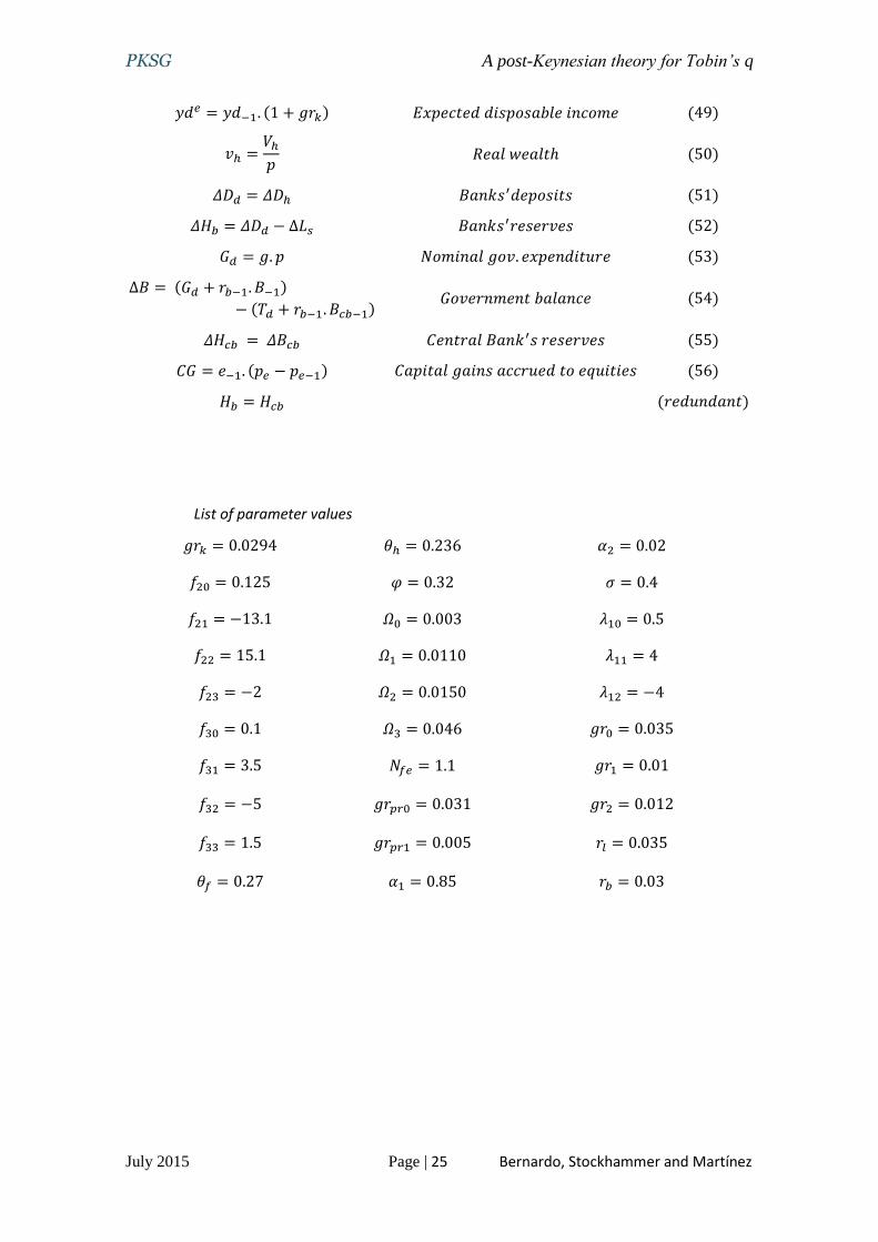
𝑦𝑑𝑒 = 𝑦𝑑−1. (1 + 𝑔𝑟𝑘) 𝐸𝑥𝑝𝑒𝑐𝑡𝑒𝑑 𝑑𝑖𝑠𝑝𝑜𝑠𝑎𝑏𝑙𝑒 𝑖𝑛𝑐𝑜𝑚𝑒 (49)
𝑣ℎ =𝑉ℎ
𝑝 𝑅𝑒𝑎𝑙 𝑤𝑒𝑎𝑙𝑡ℎ (50)
𝛥𝐷𝑑 = 𝛥𝐷ℎ 𝐵𝑎𝑛𝑘𝑠′𝑑𝑒𝑝𝑜𝑠𝑖𝑡𝑠 (51)
𝛥𝐻𝑏 = 𝛥𝐷𝑑 − ∆𝐿𝑠 𝐵𝑎𝑛𝑘𝑠′𝑟𝑒𝑠𝑒𝑟𝑣𝑒𝑠 (52)
𝐺𝑑 = 𝑔. 𝑝 𝑁𝑜𝑚𝑖𝑛𝑎𝑙 𝑔𝑜𝑣. 𝑒𝑥𝑝𝑒𝑛𝑑𝑖𝑡𝑢𝑟𝑒 (53)
∆𝐵 = (𝐺𝑑 + 𝑟𝑏−1. 𝐵−1)
− (𝑇𝑑 + 𝑟𝑏−1. 𝐵𝑐𝑏−1) 𝐺𝑜𝑣𝑒𝑟𝑛𝑚𝑒𝑛𝑡 𝑏𝑎𝑙𝑎𝑛𝑐𝑒 (54)
𝛥𝐻𝑐𝑏 = 𝛥𝐵𝑐𝑏 𝐶𝑒𝑛𝑡𝑟𝑎𝑙 𝐵𝑎𝑛𝑘′𝑠 𝑟𝑒𝑠𝑒𝑟𝑣𝑒𝑠 (55)
𝐶𝐺 = 𝑒−1. (𝑝𝑒 − 𝑝𝑒−1) 𝐶𝑎𝑝𝑖𝑡𝑎𝑙 𝑔𝑎𝑖𝑛𝑠 𝑎𝑐𝑐𝑟𝑢𝑒𝑑 𝑡𝑜 𝑒𝑞𝑢𝑖𝑡𝑖𝑒𝑠 (56)
𝐻𝑏 = 𝐻𝑐𝑏 (𝑟𝑒𝑑𝑢𝑛𝑑𝑎𝑛𝑡)
List of parameter values
𝑔𝑟𝑘 = 0.0294 𝜃ℎ = 0.236 𝛼2 = 0.02
𝑓20 = 0.125 𝜑 = 0.32 𝜎 = 0.4
𝑓21 = −13.1 𝛺0 = 0.003 𝜆10 = 0.5
𝑓22 = 15.1 𝛺1 = 0.0110 𝜆11 = 4
𝑓23 = −2 𝛺2 = 0.0150 𝜆12 = −4
𝑓30 = 0.1 𝛺3 = 0.046 𝑔𝑟0 = 0.035
𝑓31 = 3.5 𝑁𝑓𝑒 = 1.1 𝑔𝑟1 = 0.01
𝑓32 = −5 𝑔𝑟𝑝𝑟0 = 0.031 𝑔𝑟2 = 0.012
𝑓33 = 1.5 𝑔𝑟𝑝𝑟1 = 0.005 𝑟𝑙 = 0.035
𝜃𝑓 = 0.27 𝛼1 = 0.85 𝑟𝑏 = 0.03
PKSG A post-Keynesian theory for Tobin’s q
July 2015 Page | 26 Bernardo, Stockhammer and Martínez
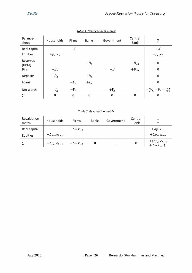
Table 1. Balance-sheet matrix
Balance-sheet
Households Firms Banks Government Central
Bank ∑
Real capital +𝐾 +𝐾
Equities +𝑝𝑒 . 𝑒ℎ +𝑝𝑒 . 𝑒ℎ
Reserves (HPM)
+𝐻𝑏 −𝐻𝑐𝑏 0
Bills +𝐵ℎ −𝐵 +𝐵𝑐𝑏 0
Deposits +𝐷ℎ −𝐷𝑑 0
Loans −𝐿𝑑 +𝐿𝑠 0
Net worth −𝑉ℎ −𝑉𝑓 − +𝑉𝑔 − −(𝑉ℎ + 𝑉𝑓 − 𝑉𝑔)
∑ 0 0 0 0 0 0
Table 2. Revaluation matrix
Revaluation matrix
Households Firms Banks Government Central
Bank ∑
Real capital +∆𝑝. 𝑘−1 +∆𝑝. 𝑘−1
Equities +∆𝑝𝑒 . 𝑒ℎ−1 +∆𝑝𝑒 . 𝑒ℎ−1
∑ +∆𝑝𝑒 . 𝑒ℎ−1 +∆𝑝. 𝑘−1 0 0 0 +(∆𝑝𝑒 . 𝑒ℎ−1
+ ∆𝑝. 𝑘−1)
PKSG A post-Keynesian theory for Tobin’s q
July 2015 Page | 27 Bernardo, Stockhammer and Martínez
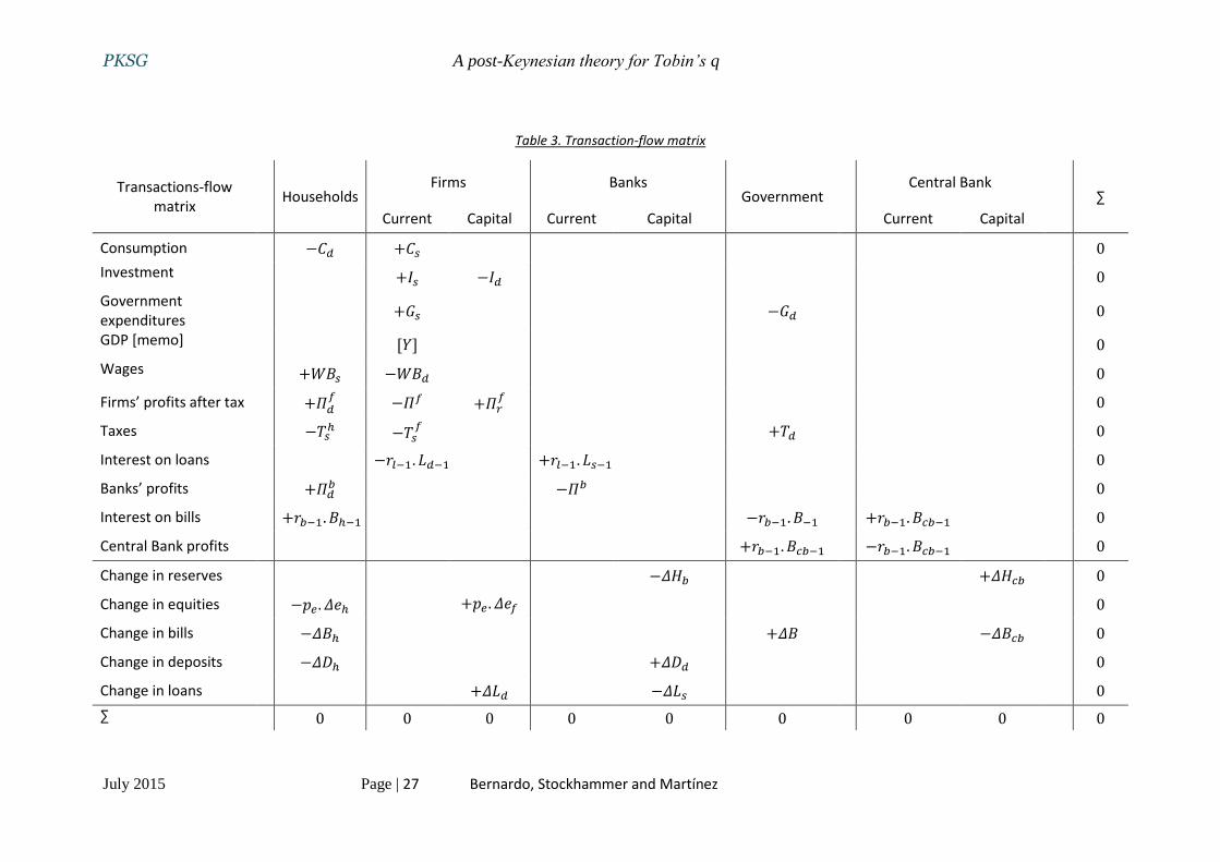
Table 3. Transaction-flow matrix
Transactions-flow matrix
Households Firms Banks
Government Central Bank
∑
Current Capital Current Capital Current Capital
Consumption −𝐶𝑑 +𝐶𝑠 0
Investment +𝐼𝑠 −𝐼𝑑 0
Government expenditures
+𝐺𝑠 −𝐺𝑑 0
GDP [memo] [𝑌] 0
Wages +𝑊𝐵𝑠 −𝑊𝐵𝑑 0
Firms’ profits after tax +𝛱𝑑𝑓
−𝛱𝑓 +𝛱𝑟𝑓
0
Taxes −𝑇𝑠ℎ −𝑇𝑠
𝑓 +𝑇𝑑 0
Interest on loans −𝑟𝑙−1. 𝐿𝑑−1 +𝑟𝑙−1. 𝐿𝑠−1 0
Banks’ profits +𝛱𝑑𝑏 −𝛱𝑏 0
Interest on bills +𝑟𝑏−1. 𝐵ℎ−1 −𝑟𝑏−1. 𝐵−1 +𝑟𝑏−1. 𝐵𝑐𝑏−1 0
Central Bank profits +𝑟𝑏−1. 𝐵𝑐𝑏−1 −𝑟𝑏−1. 𝐵𝑐𝑏−1 0
Change in reserves −𝛥𝐻𝑏 +𝛥𝐻𝑐𝑏 0
Change in equities −𝑝𝑒 . 𝛥𝑒ℎ +𝑝𝑒 . 𝛥𝑒𝑓 0
Change in bills −𝛥𝐵ℎ +𝛥𝐵 −𝛥𝐵𝑐𝑏 0
Change in deposits −𝛥𝐷ℎ +𝛥𝐷𝑑 0
Change in loans +𝛥𝐿𝑑 −𝛥𝐿𝑠 0
∑ 0 0 0 0 0 0 0 0 0
PKSG A post-Keynesian theory for Tobin’s q
July 2015 Page | 28 Bernardo, Stockhammer and Martínez
Appendix II. Equity valuation scenarios for the M&M theorem
The main assumptions for our equity valuation exercise are as follows.
In order to value the stock, a method of residual earnings is used, given that in one scenario
the pay-out is zero, so a Gordon-dividend model (Gordon & Shapiro, 1956) would not perform
the task, given that there are no dividends to discount. In the residual earnings method, the
value of a stock is the sum of current book value plus future discounted residual earnings,
which are defined as the difference between the return on equity, 𝑟, and the equity yield, 𝛾,
times previous period book value (Penman, 2011). Because the firm in question is an ongoing
concern, a terminal value has to be added in order to take into account the part of value
accruing in the distant future; for such terminal value, a formula for continuous compounding
growth is applied. In any case, it is important to note that the residual earnings valuation
model is financially equivalent to the sum of the discounted book value, plus the discount
value of dividends in the projected horizon plus the value of discounted residual earnings
beyond the projected horizon. The tables below show that both methods yield the same
results.
For simplicity, it is assumed that future earnings are known with certainty. It is not implied
whatsoever that in the real world equity analysts face such an easy task, but rather it is a
useful device for assessing a stock’s intrinsic value – the common assumption in the M&M
literature. Book value is equity at historic cost in the balance sheet. The difference between
earnings and dividends in every period cumulates into the book value figure. The return on
equity, the level of current earnings divided by the book value of the previous period, is 7%,
and is equal to the equity yield in the first two scenarios – in the other two scenarios the
equity yield is lower than the return on equity.
Table 5 reports the first two valuation scenarios. The first scenario assumes a valuation with a
nil pay-out ratio. Starting with a book value of 100, this book value will be increased through
retained earnings. Although the book value increases every year, residual earnings are every
year zero (because of the assumption 𝑟 = 𝛾), so that the value of this stock is simply the book
value. On the other hand, the second scenario is assumed that dividends are paid in full. In
such a case, the book value remains flat sine die because dividends flow out of the company. It
can be seen that dividend policy in both scenarios does not matter, because the value of the
company remains unchanged.
Table 6 shows a similar story but now for 𝑟 ≠ 𝛾. It can be seen that in this case dividend policy
matters, because the value of the company is affected by the change in dividend policy – from
a value of 116.7 with a full pay-out ratio to a value of 140 with 50% as a pay-out ratio).
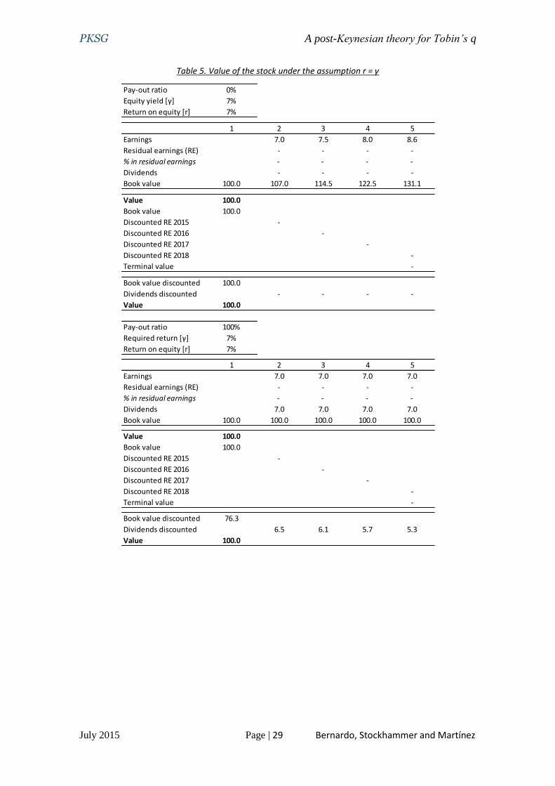
PKSG A post-Keynesian theory for Tobin’s q
July 2015 Page | 29 Bernardo, Stockhammer and Martínez
Table 5. Value of the stock under the assumption r = γ
Pay-out ratio 0%
Equity yield [γ] 7%
Return on equity [r] 7%
1 2 3 4 5
Earnings 7.0 7.5 8.0 8.6
Residual earnings (RE) - - - -
% in residual earnings - - - -
Dividends - - - -
Book value 100.0 107.0 114.5 122.5 131.1
Value 100.0
Book value 100.0
Discounted RE 2015 -
Discounted RE 2016 -
Discounted RE 2017 -
Discounted RE 2018 -
Terminal value -
Book value discounted 100.0
Dividends discounted - - - -
Value 100.0
Pay-out ratio 100%
Required return [γ] 7%
Return on equity [r] 7%
1 2 3 4 5
Earnings 7.0 7.0 7.0 7.0
Residual earnings (RE) - - - -
% in residual earnings - - - -
Dividends 7.0 7.0 7.0 7.0
Book value 100.0 100.0 100.0 100.0 100.0
Value 100.0
Book value 100.0
Discounted RE 2015 -
Discounted RE 2016 -
Discounted RE 2017 -
Discounted RE 2018 -
Terminal value -
Book value discounted 76.3
Dividends discounted 6.5 6.1 5.7 5.3
Value 100.0
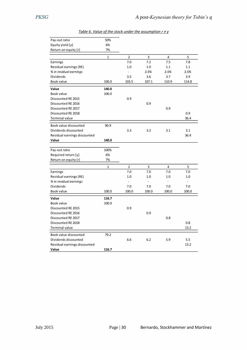
PKSG A post-Keynesian theory for Tobin’s q
July 2015 Page | 30 Bernardo, Stockhammer and Martínez
Table 6. Value of the stock under the assumption r ≠ γ
Pay-out ratio 50%
Equity yield [γ] 6%
Return on equity [r] 7%
1 2 3 4 5
Earnings 7.0 7.2 7.5 7.8
Residual earnings (RE) 1.0 1.0 1.1 1.1
% in residual earnings - 3.5% 3.5% 3.5%
Dividends 3.5 3.6 3.7 3.9
Book value 100.0 103.5 107.1 110.9 114.8
Value 140.0
Book value 100.0
Discounted RE 2015 0.9
Discounted RE 2016 0.9
Discounted RE 2017 0.9
Discounted RE 2018 0.9
Terminal value 36.4
Book value discounted 90.9
Dividends discounted 3.3 3.2 3.1 3.1
Residual earnings discounted 36.4
Value 140.0
Pay-out ratio 100%
Required return [γ] 6%
Return on equity [r] 7%
1 2 3 4 5
Earnings 7.0 7.0 7.0 7.0
Residual earnings (RE) 1.0 1.0 1.0 1.0
% in residual earnings - - - -
Dividends 7.0 7.0 7.0 7.0
Book value 100.0 100.0 100.0 100.0 100.0
Value 116.7
Book value 100.0
Discounted RE 2015 0.9
Discounted RE 2016 0.9
Discounted RE 2017 0.8
Discounted RE 2018 0.8
Terminal value 13.2
Book value discounted 79.2
Dividends discounted 6.6 6.2 5.9 5.5
Residual earnings discounted 13.2
Value 116.7