A Posteriori Error Analysis and Adaptive

Methods for Partial Differential Equations

Zhiming Chen∗

Abstract. The adaptive finite element method based on a posteriori error estimatesprovides a systematic way to refine or coarsen the meshes according to the local a poste-riori error estimator on the elements. One of the remarkable properties of the method isthat for appropriately designed adaptive finite element procedures, the meshes and theassociated numerical complexity are quasi-optimal in the sense that the finite elementdiscretization error is proportional to N−1/2 in terms of the energy norm, where N is thenumber of degrees of freedom of the underlying mesh. The purpose of this paper is toreport some of the recent advances in the a posteriori error analysis and adaptive finiteelement methods for partial differential equations. Emphases will be paid on an adaptiveperfectly matched layer technique for scattering problems and a sharp L1 a posteriorierror analysis for nonlinear convection-diffusion problems.

Mathematics Subject Classification (2000). Primary 65N15; Secondary 65N30.

Keywords. A posteriori error estimates, adaptivity, quasi-optimality

1. Introduction

The aim of the adaptive finite element method (AFEM) for solving partial differ-ential equations is to find the finite element solution and the corresponding meshwith least possible number of elements with respect to discrete errors. The task tofind the mesh with the desired property is highly nontrivial because the solutionis a priori unknown. The basic idea of the seminal work [3] is to find the desiredmesh under the principle of error equidistribution, that is, the discretization errorshould be approximately equal on each element. The error on the elements whichis also unknown can, however, can be estimated by a posteriori error estimates.Today AFEM based on a posteriori error estimates attracts increasing interestsand becomes one of the central themes of scientific computation. The purpose ofthis paper is to report some of the recent advances in the a posteriori error analysisand AFEM for partial differential equations.

A posteriori error estimates are computable quantities in terms of the discretesolution and data, which provide information for adaptive mesh refinement (andcoarsening), error control, and equidistribution of the computational effort. We

∗The author is grateful to the support of China National Basic Research Program under thegrant 2005CB321701 and the China NSF under the grant 1002510 and 10428105.

2 Zhiming Chen

now describe briefly the basic idea of AFEM using the example of solving thePossion equation on a polygonal domain Ω in R2

−Δu = f in Ω, u = 0 on ∂Ω. (1.1)

Here the source function f is assumed to be in L2(Ω). It is well-known that thesolution of the problem (1.1) may be singular due to the reentrant corners of thedomain in which case the standard finite element methods with uniform meshesare not efficient.

Let Mh be a regular triangulation of the domain Ω and Bh be the collectionof all inter-element sides of Mh. Denote by uh the piecewise linear conformingfinite element solution over Mh. For any inter-element side e ∈ Bh, let Ωe be thecollection of two elements sharing e and define the local error indicator ηe as

η2e :=

∑K∈Ωe

‖ hKf ‖2L2(K) + ‖ h1/2

e Je ‖2L2(e),

where hK := diam(K), he := diam(e), and Je := [[∇uh ]]e · ν stands for the jumpof flux across side e which is independent of the orientation of the unit normal νto e. The following a posteriori error estimate is well-known [2]

‖ u − uh ‖2H1(Ω) ≤ C

∑e∈Bh

η2e .

That ηe really indicates the error is explained by the following lower bound [39].

η2e ≤ C

∑K∈Ωe

‖ u − uh ‖2L2(K) + C

∑K∈Ωe

‖ hK(f − fK) ‖2L2(K),

where fK = 1|K|∫

K fdx.Based on the local error indicator, the usual adaptive algorithm solving the

elliptic problem (1.1) reads as follows

Solve → Estimate → Refine.

The important convergence property, which guarantees the iterative loop termi-nates in finite steps starting from an initial coarse mesh, is proved in [23, 30]. It isalso observed (cf. e.g. [30]) that for appropriately designed adaptive finite elementprocedures, the meshes and the associated numerical complexity are quasi-optimalin the sense that

‖∇(u − uh) ‖L2(Ω) ≈ CN−1/2 (1.2)

is valid asymptotically, where N is the number of elements of the underlying finiteelement mesh. Since the nonlinear approximation theory [5] indicates that N−1/2

is the highest attainable convergence order for approximating functions in H1(Ω)in two space dimensions over a mesh with N elements, one concludes that AFEMis an optimal discretization method for solving the elliptic problem (1.1).

Adaptive Finite Element Methods 3

In section 2 we consider to use AFEM to solve the Helmholtz-type scatteringproblems with perfectly conducting boundary

Δu + k2u = 0 in R2\D, (1.3a)∂u

∂n= −g on ΓD, (1.3b)

√r

(∂u

∂r− iku

)→ 0 as r = |x| → ∞. (1.3c)

Here D ⊂ R2 is a bounded domain with Lipschitz boundary ΓD, g ∈ H−1/2(ΓD)is determined by the incoming wave, and n is the unit outer normal to ΓD. We as-sume the wave number k ∈ R is a constant. We study an adaptive perfectly matchedlayer (APML) technique to deal with the Sommerfeld radiation condition (1.3c)in which the PML parameters such as the thickness of the layer and the fictitiousmedium property are determined through sharp a posteriori error estimates. TheAPML technique combined with AFEM provides a complete numerical method forsolving the scattering problem in the framework of finite element which has thenice property that the total computational costs are insensitive to the thicknessof the PML absorbing layers. The quasi-optimality of underlying FEM meshes isalso observed.

Things become much more complicated when applying AFEM to solve time-dependent partial differential equations. One important question is if one shoulduse the adaptive time marching (ATM) method in which variable timestep sizes(but constant at each time step) and variable space meshes at different time stepsare assumed, or one should consider the the space-time adaptive method in whichspace-time domain is considered as a whole and AFEM is used without distinguish-ing the difference of time and space variables. Our recent studies in [9, 10, 11] revealthat with sharp a posteriori error analysis and carefully designed adaptive algo-rithms, the ATM method also produces the very desirable quasi-optimal decay ofthe error with respect to the computational complexity

|||u − U |||Ω×(0,T ) ≤ CM−1/3 (1.4)

for a large class of convection-diffusion parabolic problems in two space dimen-sions using backward Euler scheme in time and conforming piecewise linear finiteelements in space. Here |||u − U |||Ω×(0,T ) is the energy norm of the error betweenthe exact solution u and the discrete solution U , and M is the sum of the num-ber of elements of the space meshes over all time steps. Thus if one takes thequasi-optimality of the computational complexity as the criterion to assess theadaptive methods, then the space-time adaptive method which is less studied inthe literature will not have much advantage over the ATM method.

A posteriori error analysis for parabolic problems in the framework of ATM hasbeen studied intensively in the literature. The main tool in deriving a posteriorierror estimates in [25, 26, 14, 31, 7] is the analysis of linear dual problems of thecorresponding error equations. The derived a posteriori error estimates, however,

4 Zhiming Chen

depend on the H2 regularity assumption on the underlying elliptic operator. With-out using this regularity assumption, energy method is used in [34, 10] to derive ana posteriori error estimate for the total energy error of the approximate solutionfor linear heat equations. A lower bound for the local error is also derived for theassociated a posteriori error indicator in [34, 9]. In [9] an adaptive algorithm isconstructed which at each time step, is able to reduce the error indicators (andthus the error) below any given tolerance within finite number of iteration steps.Moreover, the adaptive algorithm is quasi-optimal in terms of energy norm. In[10] an quasi-optimal ATM method in terms of the energy norm is obtained forthe linear convection-dominated diffusion problems based on L1 a posteriori errorestimates.

In section 3 we study the ATM method for the initial boundary value problemsof nonlinear convection-diffusion equations of the form

∂u

∂t+ divf(u) − ΔA(u) = g.

We derive sharp L∞(L1) a posteriori error estimates under the non-degeneracyassumption A′(s) > 0 for any s ∈ R. The problem displays both parabolic andhyperbolic behavior in a way that depends on the solution itself. It is discretizedimplicitly in time via the method of characteristic and in space via continuouspiecewise linear finite elements. The analysis is based on the Kruzkov “doublingof variables” device and the recently introduced “boundary layer sequence” tech-nique to derive the entropy error inequality on bounded domains. The derived aposteriori error estimate leads to a quasi-optimal adaptive method in terms of thenorm ‖ · ‖L1 in (1.4).

2. The APML technique for scattering problems

In this section we consider the APML technique for the scattering problem (1.3a)-(1.3c). Since [4] proposed a PML technique for solving the time dependent Maxwellequations, various constructions of PML absorbing layers have been proposed andstudied in the literature [38, 37]. Here we introduce the PML technique for (1.3a)-(1.3c) following the method in [19].

Let D be contained in the interior of the circle BR = {x ∈ R2 : |x| < R}. Inthe domain R2\BR, the solution u of (1.3a)-(1.3c) can be written under the polarcoordinates as follows

u(r, θ) =∑n∈Z

H (1)n (kr)

H (1)n (kR)

uneinθ, un =12π

∫ 2π

0

u(R, θ)e−inθdθ. (2.1)

where H (1)n is the Hankel function of the first kind and order n. The series in (2.1)

converges uniformly for r > R [20].The basic idea of PML technique is to surround the fixed domain ΩR = BR\D

with a PML layer of thickness ρ−R and choose the fictitious medium property so

Adaptive Finite Element Methods 5

that either the wave never reaches its external boundary or the amplitude of thereflected wave is so small that it does not essentially contaminate the solution inΩR.

Let α = 1+ iσ be the model medium property satisfying σ ∈ C(R), σ ≥ 0, andσ = 0 for r ≤ R. The most widely used model medium property σ in the literatureis the power function, that is,

σ = σ0

(r − R

ρ − R

)m

, m ≥ 1, σ0 > 0 constant. (2.2)

Denote by r the complex radius defined by

r = r(r) ={

r if r ≤ R,∫ r

0α(t)dt = rβ(r) if r ≥ R.

Since H (1)n (z) ∼

√2

πz ei(z−π2 n−π

4 ) as |z| → ∞, [19] obtained the PML equation by

considering the following extension of u in the exterior domain R2\BR

w(r, θ) =∑n∈Z

H (1)n (kr)

H (1)n (kR)

uneinθ, un =12π

∫ 2π

0

u(R, θ)e−inθdθ. (2.3)

It is easy to check that w satisfies

∇ · (A∇w) + αβk2w = 0 in R2\BR,

where A = A(x) is a matrix which satisfies, in polar coordinates,

∇ · (A∇) =1r

∂

∂r

(βr

α

∂

∂r

)+

α

β

1r2

∂2

∂θ2.

The PML problem then becomes

∇ · (A∇u) + αβk2u = 0 in Bρ\D, (2.4a)∂u

∂n= −g on ΓD, u = 0 on Γρ. (2.4b)

It is proved in [22, 21] that the resultant PML solution converges exponentiallyto the solution of the original scattering problem as the thickness of the PMLlayer tends to infinity. We remark that in practical applications involving PMLtechniques, one cannot afford to use a very thick PML layer if uniform finiteelement meshes are used because it requires excessive grid points and hence morecomputer time and more storage. On the other hand, a thin PML layer requires arapid variation of the artificial material property which deteriorates the accuracyif too coarse mesh is used in the PML layer.

The APML technique was first proposed in [16] for solving scattering by pe-riodic structures (the grating problem) which uses a posteriori error estimates todetermine the PML parameters such as the thickness and the medium property

6 Zhiming Chen

like σ0 in the (2.2). For the scattering problem (1.3a)-(1.3c), the main difficultyof the analysis is that in contrast to the grating problems in which there are onlyfinite number of outgoing modes [16], now there are infinite number of outgoingmodes expressed in terms of Hankel functions. We overcome this difficulty by theby exploiting the following uniform estimate for the Hankel functions H1

ν , ν ∈ R.

Lemma 2.1. For any ν ∈ R, z ∈ C++ = {z ∈ C : (z) ≥ 0,�(z) ≥ 0}, and Θ ∈ Rsuch that 0 < Θ ≤ |z|, we have

|H (1)ν (z)| ≤ e

−�(z)“1− Θ2

|z|2”1/2

|H (1)ν (Θ)|.

The proof of the lemma which depends on the Macdonald formula for themodified Bessel functions can be found in [16]. Lemma 2.1 allows us to provethe exponentially decaying property of the PML solution without resorting to theintegral equation technique in [22] or the representation formula in [21]. As acorollary of Lemma 2.1, we know that the function w in (2.3) satisfies

‖w ‖H1/2(Γρ) ≤ e−k�(ρ)

“1− R2

|ρ|2”1/2

‖ u ‖H1/2(ΓR).

We remark that in [22], [21], it is required that the fictitious absorbing coeffi-cient must be linear after certain distance away from the boundary where the PMLlayer is placed. We also remark that since (2.5) is valid for all real order ν, theresults of [12] can be extended directly to study three dimensional Helmholtz-typescattering problems.

Let Mh be a regular triangulation of Bρ\D and uh be the finite element solutionof the PML problem (2.4a)-(2.4b). Let Bh denote the set of all sides that do notlie on ΓD and Γh

ρ . For any K ∈ Mh, we introduce the residual:

Rh := ∇ · (A∇uh|K) + αβk2uh|K .

For any interior side e ∈ Bh which is the common side of K1 and K2 ∈ Mh, wedefine the jump residual across e:

Je := (A∇uh|K1 − A∇uh|K2) · νe,

using the convention that the unit normal vector νe to e points from K2 to K1. Ife = ΓD ∩ ∂K for some element K ∈ Mh, then we define the jump residual

Je := 2(∇uh|K · n + g)

For any K ∈ Mh, denote by ηK the local error estimator which is defined by

ηK

= maxx∈K

ω(x) ·(‖hKRh‖2

L2(K) +12

∑e⊂∂K

he‖ Je ‖2L2(e)

)1/2

,

where K is the union of all elements having nonempty intersection with K, and

ω(x) =

{1 if x ∈ BR\D,

|α0α|e−k�(r)“1− r2

|r|2”1/2

if x ∈ Bρ\BR,

Adaptive Finite Element Methods 7

Theorem 2.2. There exists a constant C depending only on the minimum angleof the mesh Mh such that the following a posterior error estimate is valid

‖ u − uh ‖H1(ΩR) ≤ CΛ(kR)1/2(1 + kR)

( ∑K∈Mh

η2K

)1/2

+C(1 + kR)2|α0|2e−k�(ρ)“1− R2

|ρ|2”1/2

‖ uh ‖H1/2(ΓR).

Here Λ(kR) = max

(1,

|H(1)0

′(kR)||H(1)

0 (kR)|

).

From Theorem 3.1 we know that the a posteriori error estimate consists of twoparts: the PML error and the finite element discretization error. An adaptivealgorithm is developed in [12] which uses the a posteriori error estimate to deter-mine the PML parameters. We first choose ρ and σ0 such that the exponentiallydecaying factor

ω = e−k�(ρ)(1− R2

|ρ|2 )1/2

≤ 10−8,

which makes the PML error negligible compared with the finite element discretiza-tion errors. Once the PML region and the medium property are fixed, we usethe standard finite element adaptive strategy to modify the mesh according to thea posteriori error estimate. The extensive numerical experiments reported in [12]show the competitive behavior of the proposed adaptive method. In particular, thequasi-optimality of meshes is observed and the adaptive algorithm is robust withrespect to the choice of the thickness of PML layer: the far fields of the scatteringsolutions are insensitive to the choices of the PML parameters.

3. The ATM method for nonlinear convection

diffusion problems

Let Ω is a bounded domain in Rd(d = 1, 2, 3) with Lipschitz boundary and T > 0.We consider the following nonlinear convection-diffusion equation

∂u

∂t+ divf(u) − ΔA(u) = g in Q (3.1)

with the initial and boundary conditions

u|t=0 = u0, u|∂Ω×(0,T ) = 0. (3.2)

Here u = u(x, t) ∈ R, with (x, t) ∈ Q = Ω×(0, T ). We assume that the function f :R → Rd is locally Lipschitz continuous, the function A : R → R is nondecreasingand locally Lipschitz continuous, g ∈ L∞(Q) and u0 ∈ L∞(Ω).

Problems of the type (3.1) model a wide variety of physical phenomena in-cluding porous media flow, flow of glaciers and sedimentation processes, or flow

8 Zhiming Chen

transport through unsaturated porous media which is governed by the so-calledRichards equation. For the Richards equation, the existence of weak solutions isconsidered in [1] and the uniqueness of weak solutions is proved in [33] based onthe Kruzkov “doubling of variables” technique. Entropy solutions for (3.1) arestudied in [6, 29].

The discretization of (3.1) is based on combining continuous piecewise linearfinite elements in space with the characteristic finite difference in time. The methodof characteristic originally proposed in [24, 35] is widely used to solve convection-diffusion problems in finite element community (cf. e.g. [26, 14]). Given Un−1

h

as the finite element approximation of the solution at time tn−1, let τn and V n0 ⊂

H10 (Ω) be the time step and the conforming linear finite element space at the nth

time step, then our discrete scheme reads as following: find Unh ∈ V n

0 such that

⟨Un

h − Un−1h

τn, v

⟩+ 〈∇A(Un

h ),∇v〉 = 〈gn, v〉 ∀v ∈ V n0 , (3.3)

where gn = τ−1n

∫ tn

tn−1 g(x, t)dt, Un−1h (x) = Un−1

h (X(tn−1)), and the approximatecharacteristic X(t) is defined by

dX/dt = f ′(Un−1h (X(t))), X(tn) = x.

The well-known Kruzkov “doubling of variables” technique originally appearedin [28] plays a decisive role in the error estimation (both a posteriori and a priori)for numerical schemes solving the Cauchy problems of nonlinear conservation laws(see e.g. [17, 18, 27] and the reference therein). It is also used recently in [32] forthe implicit vortex centered finite volume discretization of the Cauchy problemsof (3.1) for general non-negative A′(s) ≥ 0 for all s ∈ R. The common feature ofthese studies is that the derived error indicators are of the order

√h in the region

where the solution is smooth, where h is the local mesh size. We remark that inthe region where the diffusion is dominant, the error indicators developed for theparabolic equations (cf. e.g. [34, 9]) are of order h. Thus the degeneration ofthe order of the error indicators used in [32] may cause over-refinements for thesolution of (3.1) in the region where the diffusion is dominant.

The basic assumption in this paper is that the diffusion is positive

A′(s) > 0, ∀s ∈ R.

This assumption includes the Richards equation and the viscosity regularizationof degenerate parabolic equations, for example, the regularized continuous castingproblem which is considered in [14]. The novelty of our analysis with respect tothe analysis for nonlinear conservation laws in [17, 18, 27] or nonlinear degenerateparabolic equations in [32] lies in the following aspects. Firstly, only Cauchyproblems are considered in [17, 18, 27, 32]. The difficulty to include boundarycondition is essential. Here we use the recently introduced technique of “boundarylayer sequence” in [29] to overcome the difficulty. The technique of “boundary layersequence” allows us to truncate the standard Kruzkov test function (see Definition

Adaptive Finite Element Methods 9

3.4 below) to obtain the admissible test function in the entropy error identity.Secondly, the nature of the estimators are different: our estimators emphasize thediffusion effect of the problem which requires the assumption A′(s) > 0 for anys ∈ R; the estimates in [32] are valid for any nonlinear function A such thatA′(s) ≥ 0. The nice consequence of the analysis is that our a posteriori errorestimates are able to recover the standard sharp a posteriori error estimators inthe literature derived for parabolic problem with diffusion coefficients boundeduniformly away from zero.

Now we elaborate the main steps to derive sharp L1 a posteriori error estimatefor the discrete scheme (3.3) based on the Kruzkov “doubling of variables” device.By testing (3.1) with any function ϕ ∈ L2(0, T ; H1

0(Ω)) such that φ(·, 0) = φ(·, T ) =0, we have

∫ T

0

〈∂tu, ϕ〉dt +∫

Q

(−f(u) + ∇A(u)) · ∇ϕdxdt =∫

Q

gϕdxdt. (3.4)

For any ε > 0, let

Hε(z) = sgn(z)min(1, |z|/ε)

be the regularization of the sign function sgn(z). For any k ∈ R, define the entropypair (Uε, Fε) by

Uε(z, k) =∫ z

k

Hε(A(r) − A(k))dr, Fε(z, k) =∫ z

k

Hε(A(r) − A(k))f ′(r)dr.

The following result is well-known (cf. e.g. [6, 29]) by taking ϕ = Hε(A(u)−A(k))φin (3.4).

Lemma 3.1. For any φ ∈ L2(0, T ; H10 (Ω)) such that φ(·, 0) = φ(·, T ) = 0, and

any k ∈ R, we have

−∫

Q

Uε(u, k)∂tφ −∫

Q

Fε(u, k) · ∇φ +∫

Q

Hε(A(u) − A(k))∇A(u) · ∇φ

+∫

Q

H ′ε(A(u) − A(k))|∇A(u)|2φ =

∫Q

gHε(A(u) − A(k))φ. (3.5)

Let (H1(Ω))′ be the dual space of H1(Ω), we define the discrete residual R ∈L2(0, T ; (H1(Ω))′) through the following relation, for any ϕ ∈ H1(Ω),

〈∂tUh, ϕ〉 − 〈f(Uh),∇ϕ〉 + 〈∇A(Uh),∇ϕ〉 = 〈g, ϕ〉 − 〈R, ϕ〉. (3.6)

For any k′ ∈ R, by taking ϕ = Hε(A(Uh) − A(k′))φ in (3.6), we have thefollowing result.

10 Zhiming Chen

Lemma 3.2. For any φ ∈ L2(0, T ; H10 (Ω)) such that φ(·, 0) = φ(·, T ) = 0, and

any k′ ∈ R, we have

−∫

Q

Uε(Uh, k′)∂tφ −∫

Q

Fε(Uh, k′) · ∇φ +∫

Q

Hε(A(Uh) − A(k′))∇A(u) · ∇φ

+∫

Q

H ′ε(A(Uh) − A(k′))|∇A(Uh)|2φ

=∫

Q

gHε(A(Uh) − A(k′))φ −∫ T

0

〈R, Hε(A(Uh) − A(k′))φ〉. (3.7)

Now we are going to apply the Kruzkov “doubling of variables” technique andwill always write u = u(y, s), Uh = Uh(x, t), unless otherwise stated. By takingk = Uh(x, t) in (3.5) and k′ = u(y, s) in (3.7), we have the following entropy erroridentity.

Lemma 3.3. Let φ = φ(x, t; y, s) be non-negative function such that

(x, t) �→ φ(x, t; y, s) ∈ C∞c (Q) for every (y, s) ∈ Q,

(y, s) �→ φ(x, t; y, s) ∈ C∞c (Q) for every (x, t) ∈ Q.

Then we have

−∫

Q×Q

Uε(u, Uh)(∂tφ + ∂sφ) −∫

Q×Q

Fε(u, Uh)(∇xφ + ∇yφ)

+∫

Q×Q

Hε(A(u) − A(Uh))∇yA(u) · (∇xφ + ∇yφ)

+∫

Q×Q

Hε(A(Uh) − A(u))∇xA(Uh) · (∇xφ + ∇yφ)

+∫

Q×Q

H ′ε(A(u) − A(Uh))|∇xA(Uh) −∇yA(u)|2φ

= −∫

Q×Q

∂t[Uε(Uh, u) − Uε(u, Uh))]φ

−∫

Q×Q

∇x[Fε(Uh, u) − Fε(u, Uh))]φ

−∫

Q(y,s)

∫ T

0

〈R, Hε(A(Uh) − A(u))φ〉dt. (3.8)

The next objective is to remove the restriction that the test functions in theentropy error identity (3.8) must have vanishing trace. This is achieved by usingthe technique of boundary layer sequence introduced in [29]. For any δ > 0, theboundary layer sequence ζδ is defined as the solution of the elliptic problem

−δ2Δζδ + ζδ = 1 in Ω, ζδ = 0 on ∂Ω.

We specify now the choice of the test function φ in the entropy error identity(3.8), which is similar to that used in [29].

Adaptive Finite Element Methods 11

Definition 3.4. Let

φ(x, t, y, s) = ζδ(x)ζη(y)ξ(x, t, y, s)θ(t),

where θ ∈ C∞c (0, T ) such that θ ≥ 0, and ξ is defined as follows. Let {ϕj}0≤j≤J be

a partition of unity subordinate to open sets B0, B1, · · · , BJ such that Ω ⊂ ∪Jj=0Bj ,

B0 ⊂⊂ Ω and ∂Ω ⊂ ∪Jj=1Bj . Let ϕj ∈ C∞

c (Rd), 0 ≤ ϕj ≤ 1, such that supp(ϕj) ⊂Bj and ϕj(x) = 1 on the support of ϕj so that ϕj(x)ϕj(x) = ϕj(x). We use ϕj

as a function of y and ϕj as a function of x, and denote ϕj(x)ϕj(y) = ψj(x, y).Define

ξ(x, t, y, s) =J∑

j=0

ωl(t − s)ωm(x′ − y′)ωn(xd − yd)ψj(x, y),

where ωl, ωn are sequences of symmetric mollifiers in R, ωm is a sequence of sym-metric mollifier in Rd−1, and for j = 1, 2, · · · , J , x = (x′, xd), y = (y′, yd) arelocal coordinates induced by ψj(x, y) in Bj , that is, Bj ∩ ∂Ω = {x ∈ Bj : xd =ρj(x′)}, B ∩ Ω = {x ∈ Bj : xd < ρj(x′)} for some Lipschitz continuous functionρj : Rd−1 → R.

By taking limit δ, η → 0 in the entropy error identity (3.8), we obtain thefollowing entropy error inequality.

Theorem 3.5. Let θ and ξ be defined in Definition 3.4. Then we have the followingentropy error inequality

−∫

Q×Q

Uε(u, Uh)ξθt −∫

Q×Q

Kε(u, Uh) · (∇xξ + ∇yξ)θ

+∫

Q×Q

H ′ε(A(u) − A(Uh))|∇xA(Uh) −∇yA(u)|2ξθ

≤ −∫

Q×Q

∂t[Uε(Uh, u) − Uε(u, Uh))]ξθ

−∫

Q×Q

∇x[Fε(u, Uh) − Fε(u, Uh))]ξθ

−∫

Q(y,s)

∫Σ(x,t)

(Fε(u, Uh) − Hε(A(u) − A(Uh))∇yA(u)

)· νxξθ

−∫

Q(x,t)

∫Σ(y,s)

(Fε(u, Uh) − Hε(A(Uh) − A(u))∇xA(Uh)

)· νyξθ

−∫

Q(y,s)

∫ T

0

〈R, Hε(A(Uh) − A(u))ξθ〉dt, (3.9)

where Kε(u, Uh) = Fε(u, Uh)−Hε(A(u)−A(Uh))(∇yA(u)−∇xA(Uh)), Σ = ∂Ω×(0, T ), and Σ(x,t) or Σ(y,s) are the domain of integration of Σ with respect to (x, t)or (y, s) respectively.

12 Zhiming Chen

For any ε > 0 and z ∈ R, define

ν(ε, z) = min{A′(s) : |A(s) − A(z)| ≤ ε}.

Assume A′ ◦ A−1 is Lipschitz, then we have the following elementary estimatewhich extends the result in [18, Corollary 6.4]

|∂z[Uε(z, k) − Uε(k, z)]| ≤ ε

ν(ε, z)K1, |∂z[Fε(z, k) − Fε(k, z)]| ≤ ε

ν(ε, z)K2,(3.10)

where k, z ∈ R, K1 = L(A′ ◦ A−1), K2 = K1‖ f ′ ‖L∞(R) + L(f ′) with L(A′ ◦ A−1)and L(f ′) being the Lipschitz constant of A′ ◦ A−1 and f ′ respectively.

To complete the Kruzkov “doubling of variables” technique, we let first l, m →∞ then n → ∞ in the entropy error inequality (3.9). The first two terms on theright-hand side of (3.9) can be treated by using (3.10) and the third and fourthterms can be shown to tend to zero. Thus we have

−∫

Q

Uε(u, Uh)θt +∫

Q

H ′ε(A(u) − A(Uh))|∇(A(Uh) − A(u))|2θ

≤ Kε

∫Q

1ν(ε, Uh)

(|∂tUh| + |∇xUh|)θ −∫ T

0

〈R, Hε(A(Uh) − A(u))θ〉dt.

where K = max(K1,K2).To proceed, we introduce the interior residual

Rn := gn − Unh − Un−1

h

τn+ ΔA(Un

h ) on any K ∈ Mn,

where we recall that gn = τ−1n

∫ tn

tn−1 g(x, t)dt.

Theorem 3.6. Let ε0 =∑3

i=1 Ei, where E1, E2, E3 are the error indicators definedbelow. For any m ≥ 1, let Qm = Ω × (0, tm), and define

Λm = max(

1,

∫Qm

1ν(ε0, Uh)

(|∂tUh| + |∇Uh|) +∫

Ω

1ν(ε0, Um

h )

), (3.11)

where for any z ∈ R, ν(ε0, z) = min{A′(s) : |A(s) − A(z)| ≤ ε0}. Then thereexists a constant C depending only on the minimum angles of the meshes Mn,n = 1, · · · , m, such that the following a posteriori error estimate is valid

‖ um − Umh ‖L1(Ω) ≤ E0 + E4 + E5 + CΛ1/2

m

(3∑

i=1

Ei

),

Adaptive Finite Element Methods 13

where the error indicators Ei, i = 0, · · · , 5, are defined by

E0 = ‖ u0 − U0h ‖L1(Ω) initial error

E1 =

(m∑

n=1

τn|||h1/2n [[∇A(Un

h )]]|||2L2(Ω)

)1/2

jump residual

E2 =

(m∑

n=1

τn‖ hnRn ‖2L2(Ω)

)1/2

interior residual

E3 =

(m∑

n=1

τn‖∇(A(Unh ) − A(Un−1

h )) ‖2L2(Ω)

)1/2

time residual

E4 =m∑

n=1

∫ tn

tn−1

∥∥∥∥Unh − Un−1

h

τn− (∂tUh + divf(Uh))

∥∥∥∥L1(Ω)

dt characteristic

and coarsening

E5 =m∑

n=1

∫ tn

tn−1‖ g − gn ‖L1(Ω)dt source.

In the case of strong diffusion A′(s) ≥ β > 0 for any s ∈ R and A′ is uniformlyLipschitz continuous, then Λn is bounded by β−1‖Uh ‖BV (Qn) which is expected tobe bounded in practical computations. The a posteriori error estimator in Theorem3.6 then recovers the standard a posteriori error estimator derived in the literaturefor parabolic problems [34, 9]. In particular, the space error indicators En

1 , En2 ,

which control the adaptation of finite element meshes at each time step, are sharpin the sense that a local lower bound for the error can be established by extendingthe argument in [9, Theorem 2.2] for linear parabolic equations.

We also remark that the method of the a posteriori error analysis here is differ-ent from those for nonlinear conservation laws in [17, 18, 27] or nonlinear degenerateparabolic equations in [32]. Recall that there are several parameters introduced inthe analysis

• The regularizing parameter ε in Hε(z);• The boundary layer sequence parameters δ, η and the mollifier parameters

l, m, n.

The analysis for Cauchy problems in [17, 18, 27] is based on letting ε → 0and taking finite mollifier parameters l, m, n. The analysis in [32] takes both finiteε and finite mollifier parameters l, m, n. Note that there are no boundary layersequence parameters δ, η for the analysis for Cauchy problems. The analysis inthis paper is based on letting δ, η → 0 and l, m, n → ∞ but taking a finite ε. Weare not able to use the same technique as that in [17, 18, 27, 32] by choosing finitemollifier parameters l, m, n to treat the problem with boundary conditions.

Based on the a posteriori error estimate in Theorem 3.6, an adaptive algorithmis proposed and implemented in [11]. In particular, the numerical experiments in[11] indicate that the total estimated error is roughly proportional to M−1/3, i.e.

14 Zhiming Chen

η ≈ CM−1/3 for some constant C > 0. This implies the quasi-optimal decay ofthe error

‖ u − Uh ‖L∞(0,T ;L1(Ω)) +∫

Q

H ′ε(A(u) − A(Uh))|∇(A(Uh) − A(u))|2 ≤ CM−1/3

is valid asymptotically. Here M is the sume of the number of elements of the spacemeshes over all time steps.

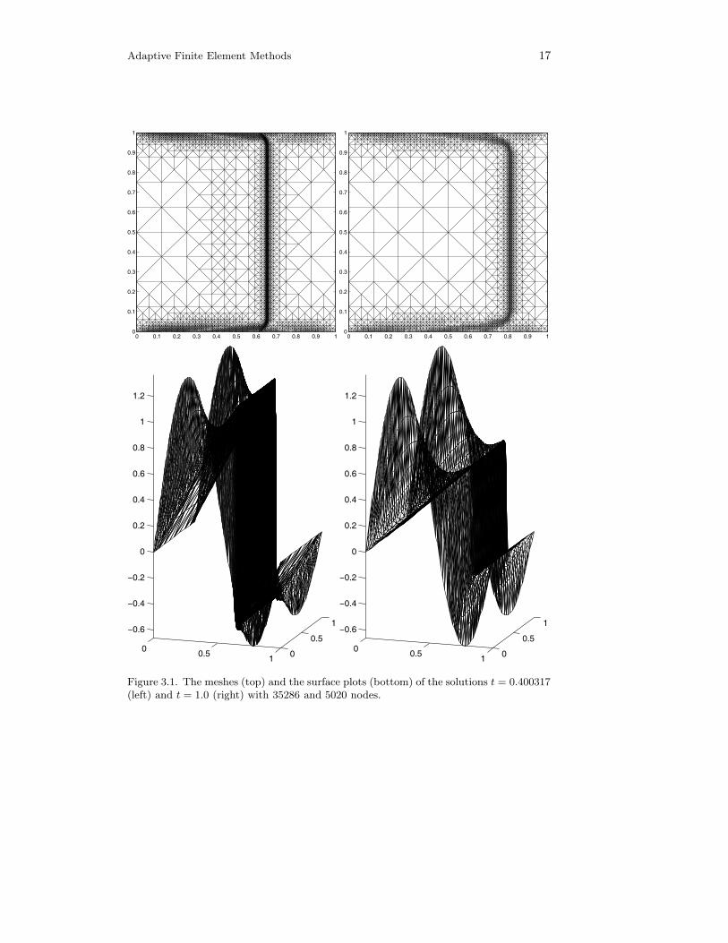
Figure 3.1 shows the meshes and the surface plots of the solutions at timet = 0.251278 and t = 0.500878 for the Burger’s equation with small viscosity

∂u

∂t+ u∂xu − εΔu = 0 in Q,

where Ω = (0, 1)2, T = 1.0, ε = 10−3, and the initial condition and boundarycondition

u(x, y, t)|∂Ω = u0(x, y) = 0.5 sin(πx) + sin(2πx).

The adaptive algorithm is based on the a posteriori error estimate in Theorem 3.6and is described in [11]. We observe from Figure 3.1 that the method captures theinternal and boundary layers of the solution.

Acknowledgment. The author would like to thank Shibin Dai, Guanghua Ji,Feng Jia, Xuezhe Liu, Ricardo H. Nochetto, Alfred Schmidt, and Haijun Wu forthe joint work through the years.

References

[1] Alt, H.W. and Luckhaus, S., Quasilinear elliptic-parabolic differential equations,Math. Z. 183 (1983), 311-341.

[2] Babuska, I. and Miller, A., A feedback finite element method with a posteriori errorestimation: Part I. The finite element method and some basic properties of the aposteriori error estimator, Comput. Meth. Appl. Mech. Engrg. 61 (1987), 1-40.

[3] Babuska, I. and Rheinboldt, C., Error estimates for adaptive finite element compu-tations, SIAM J. Numer. Anal. 15 (1978), 736-754.

[4] Berenger, J.-P., A perfectly matched layer for the absorption of electromagneticwaves. J. Comput. Physics 114 (1994), 185-200.

[5] Binev, P., Dahmen, W. and DeVore, R., Adaptive finite element methods with con-vergence rates, Numer. Math. 97 (2004), 219-268.

[6] Carrillo, J., Entropy solutions for nonlinear degenerate problems, Arch. RationalMech. Anal. 147 (1999), 269-361.

[7] Chen, Z. and Dai, S., Adaptive Galerkin methods with error control for a dynamicalGinzburg-Landau model in superconductivity, SIAM J. Numer. Anal. 38 (2001),1961-1985.

[8] Chen, Z. and Dai, S., On the efficiency of adaptive finite element methods for ellipticproblems with discontinuous coefficients. SIAM J. Sci. Comput. 24 (2002), 443-462.

Adaptive Finite Element Methods 15

[9] Chen, Z. and Jia, F., An adaptive finite element method with reliable and efficienterror control for linear parabolic problems, Math. Comp. 73 (2004), 1163-1197.

[10] Chen, Z. and Ji, G., Adaptive computation for convection dominated diffusion prob-lems, Science in China, 47 Supplement (2004), 22-31.

[11] Chen, Z. and Ji, G., Sharp L1 a posteriori error analysis for nonlinear convection-diffusion problems, Math. Comp. (to appear).

[12] Chen, Z. and Liu, X., An Adaptive Perfectly Matched Layer Technique for Time-harmonic Scattering Problems, SIAM J. Numer. Anal. (to appear).

[13] Chen, Z. and Nochetto, R.H., Residual type a posteriori error estimates for ellipticobstacke problems, Numer. Math. 84 (2000), 527-548.

[14] Chen, Z., Nochetto, R.H., and Schmidt, A., A characteristic Galerkin method withadaptive error control for continuous casting problem, Comput. Methods Appl. Mech.Engrg. 189 (2000), 249-276.

[15] Chen, Z., Nochetto, R.H., and Schmidt, A., Error control and adaptivity for a phaserelaxation model, Math. Model. Numer. Anal. 34 (2000), 775-797.

[16] Chen, Z. and Wu, H., An adaptive finite element method with perfectly matchedabsorbing layers for the wave scattering by periodic structures. SIAM J. Numer.Anal. 41, (2003), 799-826.

[17] Cockburn, B., Coquel, B.F. and Lefloch, P.G., An error estimate for finite volumemethods for multidimensional conservation laws, Math. Comp. 63 (1994), 77-103.

[18] Cockburn, B. and Gremaud, P.-A., Error estimates for finite element methods forscalar conservation laws, SIAM J. Numer. Anal. 33 (1996), 522-554.

[19] Collino, F. and Monk, P.B., The perfectly matched layer in curvilinear coordinates.SIAM J. Sci. Comput. 19 (1998), 2061-2090.

[20] Colton D. and Kress R., Integral Equation Methods in Scattering Theory. John Wiley& Sons, New York, 1983.

[21] Hohage, T., Schmidt, F. and Zschiedrich, L., Solving time-harmonic scattering prob-lems based on the pole condition. II: Convergence of the PML method. SIAM J.Math. Anal., (to appear).

[22] Lassas, M. and Somersalo, E., On the existence and convergence of the solution ofPML equations. Computing 60 (1998), 229-241.

[23] Dorfler, W., A convergent adaptive algorithm for Possion’s equations, SIAM J. Nu-mer. Anal. 33 (1996), 1106-1124.

[24] Douglas Jr., J. and Russell, T.F., Numerical methods for convection-dominated dif-fusion problem based on combining the method of characteristic with finite elementor finite difference procedures, SIAM J. Numer. Anal. 19 (1982), pp. 871-885.

[25] Eriksson, K. and Johnson, C., Adaptive finite element methods for parabolic prob-lems I: A linear model problem, SIAM J. Numer. Anal. 28 (1991), 43-77.

[26] Houston, P. and Suli, E., Adaptive Lagrange-Galerkin methods for unsteadyconvection-diffusion problems, Math. Comp. 70 (2000), 77-106.

[27] Kroner, D. and Ohlberger, M., A posteriori error estimates for upwind finite volumeschemes for nonlinear conservation laws in multi-dimensions, Math. Comp. 69 (2000),25-39.

16 Zhiming Chen

[28] Kruzkov, N.N., First order quasi-linear equations in several independent variables,Math. USSR Sbornik 10 (1970), 217-243.

[29] Mascia, C., Porretta, A. and Terracina, A., Nonhomogeneous Dirichlet problems fordegenerate parabolic-hyperbolic equations, Arch. Rational Mech. Anal. 163 (2002),87-124.

[30] Morin, P., Nochetto. R.H. and Siebert, K.G., Data oscillation and convergence ofadaptive FEM, SIAM J. Numer. Anal. 38 (2000), 466-488.

[31] Nochetto, R.H., Schmidt, A. and Verdi, C., A posteriori error estimation and adap-tivity for degenerate parabolic problems, Math. Comp. 69 (2000), 1-24.

[32] Ohlberger, M., A posteriori error estimates for vertex centered finite volume approx-imations of convection-diffusion-reaction equations, Math. Model. Numer. Anal. 35(2001), 355-387.

[33] Otto, F., L1-contraction and uniqueness for quasilinear elliptic-parabolic equations,J. Diff. Equations 131 (1996), 20-38.

[34] Picasso, M., Adaptive finite elements for a linear parabolic problem, Comput. Meth-ods Appl. Mech. Engrg. 167 (1998), 223-237.

[35] Pironneau, O., On the transport-diffusion algorithm and its application to theNavier-Stokes equations, Numer. Math. 38 (1982), pp. 309-332.

[36] Schmidt, A. and Siebert, K.G., ALBERT: An adaptive hierarchical finite ele-ment toolbox, IAM, University of Freiburg, 2000. http://www.mathematik.uni-freiburg.de/IAM/Research/projectsdz/albert.

[37] Teixeira, F.L. and Chew, W.C., Advances in the theory of perfectly matched layers.In Fast and Efficient Algorithms in Computational Electromagnetics (ed. by W.C.Chew) Artech House, Boston, 2001, 283-346.

[38] Turkel, E. and Yefet, A., Absorbing PML boundary layers for wave-like equations.Appl. Numer. Math. 27 (1998), 533-557.

[39] Verfurth, R., A Review of A Posteriori Error Estimation and adaptive Mesh Refine-ment Techniques, Teubner (1996).

LSEC, Institute of Computational Mathematics, Academy of Mathematics and Sys-tems Science, Chinese Academy of Sciences, Beijing 100080, China.

E-mail: zmchen@lsec.cc.ac.cn

Adaptive Finite Element Methods 17

0 0.1 0.2 0.3 0.4 0.5 0.6 0.7 0.8 0.9 10

0.1

0.2

0.3

0.4

0.5

0.6

0.7

0.8

0.9

1

0 0.1 0.2 0.3 0.4 0.5 0.6 0.7 0.8 0.9 10

0.1

0.2

0.3

0.4

0.5

0.6

0.7

0.8

0.9

1

0 0.51 0

0.5

1−0.6

−0.4

−0.2

0

0.2

0.4

0.6

0.8

1

1.2

0 0.51 0

0.5

1−0.6

−0.4

−0.2

0

0.2

0.4

0.6

0.8

1

1.2

Figure 3.1. The meshes (top) and the surface plots (bottom) of the solutions t = 0.400317(left) and t = 1.0 (right) with 35286 and 5020 nodes.