A posteriori error estimation for standard finite element analysis

EUEWIER

Computer methods in applied

mechanics and engineering

Comput. Methods Appl. Mech. Engrg. 163 (1998) 141-157

A posteriori error estimation for standard finite element analysis

Pedro Departamento de Matetitica Aplicada

Diez, Juan JosC Egozcue, Antonio Huerta* III, E.T.S. de Ingenieros de Caminos, Universitat Politknica de Catalunya, Campus Nord C-2,

E-08034 Barcelona, Spain

Received 10 November 1995

Abstract

A new residual type estimator based on projections of the error on subspaces of locally-supported functions is presented. The estimator is

defined by a standard element-by-element refinement. First, an approximation of the energy norm of the error is obtained solving local

problems with homogeneous Dirichlet boundary conditions. A later emichment of the estimation is performed by adding the contributions of projections on a new family of subspaces. This estimate is a lower bound of the measure of the actual error. The estimator does not need to

approximate local boundary conditions for the error equation. Therefore, computation of flux jumps is not necessary. Moreover, the

estimator can be. applied in mixed meshes containing elements of different shapes and its implementation in a standard finite element code is

straightforward. The presented results show the effectiveness of the estimator approximating both the distribution and the global measure of

the error, as well as its usefulness in adaptive procedures. 0 1998 Elsevier Science S.A. All rights reserved.

1. Introduction

It is now widely accepted that adaptive procedures are necessary for any practical Finite-Element (FE) computations [l]. Error estimation is a key feature of an adaptive procedure. An error estimator provides

information about the global quality of the solution and the distribution of the error in the domain. The global estimate assesses admissibility of the approximate solution. If it is not admissible, a new mesh must be created

following a remeshing criterion based on the error distribution. Elements are concentrated where the approximate solution is less accurate. The goal is a new solution with a uniform error distribution and a

specified global error. A priori error estimates are the main tool for the theoretical study of the FE Method but they cannot provide

practical results [2]. In order to obtain numerical approximations of the actual error, it is necessary to use a posteriori error estimators. These estimators may be classified into two families: flux projection and residual type estimators.

Flux projection estimators are derived from the original Zienkiewicz-Zhu estimator [3]. A modified version

of this estimator, based on the superconvergent patch recovery, has been introduced in [4]. The main idea of such estimators is to approximate the actual error by the difference of a smooth recovered solution and the FE solution. These estimators have a good performance if the recovered solution improves the FE approximation.

The recovery techniques are based on superconvergence results. The points where the solution has an order of convergence higher than expected are taken as sample points. Usually, superconvergence is concerned with the values of the fluxes: superconvergent points do not hold more accurate values of the main variable but only of its derivatives. Therefore, flux projection estimators can only be employed if the error is measured using norms that can be expressed in terms of the flux. This applies in the elastic mechanical model using the energy norm.

* Corresponding author. E-mail: [email protected]

0045-7825/98/$19.00 0 1998 Elsevier Science S.A. All rights reserved.

PII: SOO45-7825(98)00009-7

142 P. Diez et al. I Comput. Methods Appl. Mech. Engrg. 163 (1998) 141-157

Although these estimators have been found to be robust, see [2] and [5], the superconvergence properties are only proved in very few cases [6]. Actually, the choice of the sample points used in the recovery technique does not alter the performance of the estimator [2]. Superconvergence is not observed in meshes mixing different

element types, therefore flux projection estimates should not be used with such meshes. Moreover, the recovered

solution usually shows a poor quality near the boundaries. Nevertheless, flux projection estimators are the most

popular and they have been implemented in many commercial FE codes because of their easy implementation

and practical efficiency. Flux projection estimates can be computed using only the existing framework of any

classical FE code. Residual type estimators were first introduced by Babu’ska and Rheinboldt in [7]. The residual of the FE

solution is used as a source term in local boundary value problems associated with the error. These estimators

are defined by two factors: the selection of the local interpolation space (usually a bubble space for a p-refined reference solution) and the approximation of the boundary conditions by splitting the flux jump across the edges

of the elements. Indeed, flux jump can be thought as a weak residual. These kind of estimators have a solid

theoretical background but their results have been found to be less robust than flux-projection estimates [2]. The

biggest part of the computational cost of these estimators is taken by the flux jump computation and the flux

splitting procedure. The implementation of these estimators is not widespread. This is probably because they

need computation of specific values which are useless for the general FE analysis.

Some estimators are difficult to classify into one of these groups. The estimators introduced by Lade&e in

[8] and Ohtsubo and Kitamura in [9] build a regularized flux field and therefore they can be put into the first

class but they solve local problems associated with the residual and, consequently, they can also be seen as

residual type estimators (see [2]). These estimators present the usual disadvantages of the second family.

The estimators defined by Erikkson and Johnson in [lo] cannot be classified into one of the above groups.

They are known as extrapolation type estimators. These estimators are based on the approximation of constants

appearing in the a priori error bounds. But they are rarely implemented in commercial codes. This is probably due to the same reasons applying for residual type estimators.

A new approach to residual type estimators is introduced here. The estimates are seen as projections on

subspaces of locally-supported functions, these projections are computed by solving local problems. The

computation of flux jumps across the edges is precluded, therefore the main disadvantages of residual type

estimators do not hold. Moreover, the estimator can be applied in any kind of meshes, even if different element

types are mixed. The obtained estimate is a lower bound of the actual error. In addition, since inputs for local

problems are the same as those for the standard problem, the definition and the computation of the estimator are

easily integrated in a finite element code. The remainder of the paper is organized as follows: Section 2 presents the model problem and notation.

Section 3 is devoted to error projection computation and some local properties of projections. In Section 4 an

interior elementwise estimator is defined. Section 5 deals with the problem of improving the estimation by

defining new projection spaces in a convenient way. In Section 6 we show some examples and demonstrate the

effectiveness of the estimator.

2. Model problem

Let us consider an elliptic problem over a bounded domain 0 C Iw2 with a piecewise smooth boundary r divided into two parts f, and r,. The boundary value problem is defined in strong form as

-V*(AVu)+bu=f in 0, (la)

u =0 on r, (lb)

and

(Ah). n = g, on 4 , (lc)

where u is defined on 0 and needs to be approximated. The Dirichlet boundary condition (lb) is taken homogeneous, but, due to the linearity of (la) this is not a loss of generality, the examples will present non-homogeneous Dirichlet boundary conditions. In order to simplify the presentation, a scalar case is

P. Dkz et al. I Comput. Methods Appl. Mech. Engrg. 16.3 (1998) 141-157 143

considered in the theoretical development of the estimator. However, the extension to vectorial problems is

straightforward and plane mechanical examples with two degrees of freedom are shown in Section 6.

In order to study the weak form of the problem, equivalent to the strong form (l), several definitions are

needed. Let H’(0) denote the usual Sobolev space of functions with square-integrable derivatives and let

HLd(0) be such that Hr,(fl) = {w E H’(a) 1 w = 0 on r,}. The solution u of (1) is also the weak solution of the

following integral problem: find u in H;,(R) such that

a(u, u) = l(u)

for all u in H:d(0), where a(., *) and 1(.) are given by

(2)

a@, u) : = (Vu . AVu + buu) d0 (3)

and

The Galerkin FE solution uh belongs to a finite dimensional subspace WJ of H f,(a) and verifies (2) for all u

in Y*. The goal of error estimation is to approximate a measure of the error e, defined as e := u - u,,.

If A is a symmetric positive definite matrix and b is non-negative, see Eq. (la), then the bilinear form a(*, *) is

also symmetric positive definite and, therefore, it is a scalar product. The norm 11*/1 induced by a(*, .) is called the

energy norm; for any u, [lull := a(u, u)"'. If Eq. (1) models a physical problem, llull represents the energy

associated to the state of the system described by u. The energy norm will be used to measure the error e.

The FE solution uh is the projection of the exact solution u on ‘& according to the scalar product a(., .), in

that sense Galerkin method is said to be optimal.

In order to have information about the distribution of error over 0, local restrictions of (I.(( will be used. For a

given subdomain fik of 0 the associated local norm of the error e is

1 l/2

lle& := [a,(e,e)]"2 := (Ve.AVe+be2)dfi . (5)

In the following sections, subdomains fik are chosen as the elements of the mesh which defines the

approximating space W;, (computational mesh).

3. Error projections

An error estimate should provide local information of the error in order to describe its spatial distribution. The

computation of an error estimate must also be local; that is the computation of a local restriction of the error in a

subdomain Q only uses information in it and, eventually, in its neighborhood. Otherwise, error estimation

becomes too expensive and it could be cheaper to use a refined mesh in order to obtain a more accurate solution.

The local estimator presented in the following section is made independent of the neighbor elements by forcing

the approximation to e to vanish on the boundary. Then, in Section 5 the estimator is improved, precluding the imposition of this artificial condition. before entering in the detailed definition of a local estimator, we discuss

error projections which are the rationale of the proposed estimator. Since the weak equation (2) is well posed and the form a(*, *) is assumed to be linear on the first argument,

the error e is the only element of Hid(R) verifying

a(e,u) = f(u):= l(u)- u(uh,u) (6)

for all u in Hhd(0). Eq. (6) is the weak global equation for the error. Thus, although the error is not known, its scalar product with any given function u may be computed. That is, the projection of e on any subspace of Hid(a) can be evaluated.


Let V, be a subspace of H:,(0) of functions having their support in L$: they vanish elsewhere and,

consequently, on the boundary of ok (V, is included in HA(Q)). The subspace V, is generated by a basis of

interpolation functions S3 = {N, , . . . , N,}. Reference to index k in the notation of the elements of 23 is omitted

when it is not necessary. The projection of e on V, is denoted by ck, the element ck of V, is represented by the

column vector [E] 3 of its components on S3, the scalar product a(*, *) is represented by matrix K with generic

term K, = a(N,, Nj) (i, j = 1, . . . , n) and the linear form &a) is represented by vector [r] with generic term

[flj = Z(Nj). Finally, the projection gk is obtained by solving the linear system of equations

K[.Y]~ = $1. (7)

Then, the energy norm of ck can be computed in a straightforward manner by the expression

ll~k112 = L4T&[4~ = kl;[fl . (8)

The set of subspaces V, is orthogonal with respect to a(*, .) because all subdomains 4 (the finite elements)

have intersection with measure zero. Bessel’s inequality applies and the norms of projections ck verify

(9)

where m stands for the number of elements in the mesh.

The bound given by (9) holds even locally. Indeed, as .sk is the projection of e on V, according to the global

form a(*, *), the difference e - .sk is orthogonal to Ed, i.e. u(e - ck, ck) = 0. Moreover, this orthogonality condition also stands for the local form a,(*, *), i.e. u,(e - .+ Q) = 0, because the support of ck is included in

L&n,. Thus,

a&, e> = uk([e - 91 + ck, [e - ~~1 + qJ

= ~&,, .Q + a& - sk, e - qJ

and a lower bound for the local measure of the error is recovered

II-A = ll-dlk c II4 . (10) Accordingly, we deduce that a family of subspaces V, of HLd(0), defined over disjoint subdomains LZk (or

with null intersection), allows us to compute local projections &k such that:

l the norm of each 9 is a lower bound of the local norm of the true error, see Eq. (lo), and can be taken as a

local error estimator,

l defining E as the sum of the ek,

&:= 2 &k k=l

(11)

the global norm of E is easily computed from the local projections and gets a lower bound of the global

measure of the error ]]e]]

Ml2 = j?, IhO c 11412 T (12)

l both global and local approximations, E and the E~‘s, would be more accurate as the space V, generated by

theV,‘s,V:=V,@V.@** * @V,, is closer to Hk (iI) (asymptotic behavior of Bessel inequality (9) is given

by Parseval’s equality). The global approximatfon E is the projection of e on V. The functions of each subspace V, vanish on the boundary of J&. Then, the global approximation E associated

with a family of Vk’s, defined from a partition of 0 into subdomains ok, takes zero values at the points lying on the boundary of the J&‘s. Those are called hidden points of the global approximation. In fact, we are artificially forcing E to be zero at these points. The space V will never approximate enough Hkd(L?) if many points of the domain are hidden. In the following sections we define new families of subspaces related to other partitions of 0 in order to reduce these hidden points.

P. Diez et al. I Comput. Methods Appl. Mech. Engrg. 163 (1998) 141-157 145

4. Definition of a local estimator. Interior residuals

The definition of the local subspaces V, characterizes the family of functions Ed. The E~‘S are taken as

approximations of the local error. That is, approximations to the error inside each element 4 where the

subspace V, is defined. Local subspaces for residual type estimators have been typically defined following a p-refinement [ 1 l- 131 or an h-refinement strategy [ 141. The present estimator can follow both approaches. For the sake of simplicity we only show an h-refinement approach.

The interpolation functions Ni generating V, are defined by a discretization of the element Q. We call these

meshes elementary submeshes. In order to make computations systematic and to have a simple implementation,

we describe an elementary submesh over a reference element. Generic elementary submeshes are built applying

the isoparametric transformation to this reference elementary submesh, see Fig. 1. Then, the interpolation

functions N, are associated with the nodes of the elementary submesh discretizing Q The nodes of the

elementary submesh lying on the boundary of 4 are not introduced in the definition of V, because the functions

of V, must vanish on the boundary.

The assembly of all the elementary submesh builds up a refined mesh discretizing the whole domain 0. The

refined mesh could be used in the computation of a more accurate reference solution u,. However, the

computation of the reference solution as a global refined problem must be avoided because of the large amount

of degrees of freedom involved.

The reference solution U, is associated with a reference error, e, := U, - uh. The reference error e,. can be seen

as the projection of the actual error e on the interpolation space W generated by the global refined mesh. The

space W includes the space V (V : = V, @3 V, $. . .$ V,) because W contains the functions Ni generating each V,,

associated with the interior nodes, but also the interpolation functions associated with the nodes lying on the

boundary of each element ok. Therefore, the projection E of e on V is also the projection of e, on V and the

estimate given by E also undervaluates the norm of e,. The goal of the presented error estimator is to

approximate the global and local norms of e, without solving the global problem. In fact, E (the projection of e,

on V) is already an initial estimate of e,. The global projection E is the assembly of the local projections Ed on

each subspace V,. Each projection .Y~ is computed solving a linear system with a few degrees of freedom, thus,

with a low computational cost.

Once the subspace V, is defined by the basis B of interpolation functions N;, Eqs. (7) and (8) are used in

order to compute /l~~ll. Th e computation of the residual term [[I, defined in Eq. (6), is straightforward once uh

belongs to the reference space W. Then, uh can be expressed by the column vector [uh]% of its nodal values in

Fig. I. Reference elementary submesh (a) and induced elementary submeshes over regular (b) and arbitrary (c) meshes.

146 P. Di’ez et al. I Comput. Methods Appl. Mech. Engrg. 163 (1998) 141-157

the elementary submesh discretizing Q. Thus, a@,, Nj), see right-hand side of Eq. (6), is easily computed from the product of K and [uh]%. Finally, we get

[tl = [Zl - K[q,l s . (13)

This expression determines the right-hand side of Eq. (7) as a function of the terms appearing in the usual FE

approach of a problem. The residual, i.e. the right-hand side of Eq. (7), does not need integration of the

approximate solution, because integrals have been carried out when K was generated.

The residual term [r] associated with a subspace V, with functions defined over an element flk is called

interior residual, The estimator given by Eq. (7) with this definition of the V, is called interior estimator. The

interior estimator is characterized by the choice of the elementary submeshes.

It is very simple to define elementary submeshes for quadrilateral elements using a structured regular mesh of

the reference square, see Fig. 1. It is important to notice that although the elementary submesh is chosen

structured, the original computational mesh can be unstructured. These kind of submeshes verify that:

(a) they are simply defined on the reference element,

(b) they can represent the restriction of u,, to fik and

(c) they can be uniformly refined as far as the user wishes.

Computing the projection Ed as described in Eq. (7) is equivalent to solving a local problem in Q, with Ok

discretized by the elementary submesh and where homogeneous Diruchlet boundary conditions are imposed on

the boundary of Q.

The norm of F~ increases with the ‘size’ of the associated subspace V, and the number of degrees of freedom

of the elementary submesh. A sequence of approximations based on refined submeshes has monotonic growth

on norms and it is bounded by the norm of the exact and the reference error. Therefore, as the submesh is

refined, the norm of the projections (local and global) converges to a value which is an underestimation of the error. This underestimation could be relatively far from ]lel]i, and even from IlerJ:, due to the fact that we are forcing the approximate function to take zero values at the hidden points.

Many authors [ 1 l- 131 solve similar local problems approximating the boundary conditions. The main idea of

those estimators is to use the discontinuity (jump) of flux across the element edges to approximate flux

(Neumann) boundary conditions for the error equation, on the boundary of each Q. Different authors use

different criteria to deduce such approximations. These approximations can be expensive because they need to

compute the solution and its derivatives in points lying on the boundary of the elements. From the point of view

of the present projection approach, it is possible to take into account the information of flux jumps across edges

by computing projections on subspaces of functions defined on subdomains including the edges. In the next

section we introduce a new family of projections based on a new partition of a. Finally, we compute a new

error estimate combining the projections on the two families. Some compatibility conditions are imposed in

order to make this combination possible and to still get a lower bound.

5. Enrichment of the estimation. Overlapped meshing

Up to now, we have computed local projections 9 of the error e on subspaces V,. We have used a partition of

fl in subdomains Q (k = 1, . . . , m, namely the elements). Each subspace V, was defined by a submesh over the

subdomain Q. The norms of Ed were taken as approximations of local measures of the true error e. Local and global approximations, 9 and E, given by (S), (11) and (12), are lower bounds of the exact and reference error norms. We realized that this approximation could be poor. We would like to add new terms to the error estimation (9), in order to get closer to the exact error norm and still keep the lower bounding.

Since E is the projection of the reference error e, on the space V, e can be uniquely expressed as the sum of 6

and a function et, orthogonal to E, such that e, = 6 + e). Using the Pythagoras theorem we can write

1].# = l]eJ2 - lle:\1*, therefore th e norm of e: is the underestimation of the global reference error by the global interior estimate. The goal of the enrichment of the estimation is to approximate the forgotten part of the reference error e,’ and to add it to the first (interior) estimates. The function et belongs to VI, the orthogonal spaceofV,V:=V,@V,@.. .Ci? V,, in the reference interpolation space W. As we want to approximate e,’ by a projection, we would like to project on a subspace included in VI.


Let us consider a new partition of 0 into subdomains Al (I = 1, . . , m’). In order to make clear the difference

between the two partitions, subdomains denoted by A, are called patches, while Ok are the actual elements.

Every patch Al is discretized by a patch-submesh generating a subspace U, in H&l,). The subspaces U, are

generated in the same way as the spaces V, associated with the elements. In order to approximate the reference

error, the elements of each patch-submesh are chosen to be elements of elementary submeshes and, then also elements of the refined global mesh generating W. Patch-submeshes and elementary-submeshes share nodes and

elements.

Since subdomains A, have zero measure intersections, subspaces U, are mutually orthogonal. The projections of e, (or e) on the U,‘s can be thought of as a new family of local approximations to e, over different domains.

Let l?, be the part of U, orthogonal to the interior global estimate E. Since fi, is a restriction of U, subject to

one linear constraint, the dimension of the subspace fil is, at least, the dimension of U, minus one. Let 7, denote

the projection of the reference error e, on ol.

Since F and each v[ are orthogonal Bessel’s inequality applies again,

(14)

The orthogonality to E does not impose 0, to be included in VI. Actually, a restriction of U, ensuring

orthogonality to the space V would reduce it to the null subspace. This is due to the fact that, in general, the

dimension of the subspace U, is less than the total number of nodes which are in the elements intersecting the

corresponding A,. Since we are obtaining a lower bound of the error, we prefer to impose the minimal restriction

allowing to add the new contributions to the interior estimates as is done in Eq. (14).

We have determined a new global estimate. Now, the only hidden points are the intersections of the edges of

the two families of subdomains, that is the intersections of the boundaries of the elements and the patches,

which is obviously a smaller set than all the edges of the elements.

Nevertheless, as noted previously, we also desire to compute a local estimate to determine the spatial

variation of the error. This local estimate is an approximation of Ile,ll:, see Eq. (5). Therefore, the contribution of

all the patches Al overlapping element Ok must be taken into account. This contribution is not the complete ~~~~~~*

but the local norm restricted to Ok, namely a,(qr, v~) = Il~J~. Recall that q! has support on Al, therefore it is zero

in 0, outside its intersection with A,. Thus, an approximation of the squared local norm of the error 11e/, can be

evaluated using

ll~kll: + c IlrllllZ

where index 1 in the summation takes the values such that the

Notice that the local norm of v, (restricted to Al) is easily

patch Al overlaps the element Q.

computed using an expression similar to (8). I. However, the computation of its contribution to element Q, i.e. IlvJk, needs to identify the elements of the patch-submeshes belonging to Ok. This can be cumbersome. Therefore, in order to further simplify the

computations another approximation is performed. We refer to equally distribute the squared norm of Q /~,112,

over all the elements overlapping the patch A,. That means we are approximating the quantities defined in (15)

by

(15)

(16)

where m, is the number of elements overlapping the patch Al and index 1 has the same range of variation as in Eq. (15). This approximation looses the lower bound property, in particular when elements with small error are next to elements with large error. However, the computational benefits are important and the examples in the next section show that the lower bound property is only lost in a negligible number of elements.

It is important to notice that the orthogonality condition to the interior global approximation E can be easily implemented if the nodes of the patch-submeshes (discretization of A,) and the nodes of the elementary- submeshes (discretization Q) are the same. Then, the selection of the subdomains Al is induced by the

discretization of 4. We must choose at the same time the geometry and the meshing of A( conditioned to the

148 P. Diez et al. / Comput. Methods Appl. Mech. Engrg. I63 (1998) 141-151

Fig. 2. Node-patch submesh (shaded) associated with the regular

elementary submeshes. Fig. 3. Edge-patch submesh (shaded) and elementary submeshes

defined through a quadrilateral meshing of a triangle.

meshing of 0. The orthogonality condition becomes a linear restriction on the local solution over each patch and

it can be easily imposed by a Lagrange multiplier technique.

Finally, in order to completely define the estimator, a description of the new partition and the corresponding

patch-submeshes is needed. If we consider an interior estimator as defined in Section 4, see Fig. 1, a set of

patches centered at the nodes of the original mesh can be defined as is shown in Fig. 2. Every node has an

associated A, with vertices at the centers of adjacent elements and the middle points of the edges. The

discretization of the patches is induced by the discretization of the elements. The hidden points of the total

estimation are only the centers of the interior edges of elements. The estimator induced by this geometric

definition is denoted by nodal-patch estimator.

It is possible to create an elementary-submesh and a patch definition ensuring that the hidden points of the

total estimation are a priori chosen points, for instance the nodes of the original mesh. Fig. 3 shows how such

submeshes and patches are defined. It is worth remarking that with this geometric definition, projection v[

includes the effect of flux jump across the edge covered by the patch AI. This estimator is denoted by edge-patch

estimator.

In the definition of the estimator we have followed a particular projection strategy. In fact, we first obtain an interior projection gk over each V, and then we use the global interior approximation E to impose a restriction for

each U,. The sum of the projections &k and rlr is only a lower bound of the full projection on a global space generated by both the two families Vk’s and Ul’s. The projection strategy could theoretically fail, depending both on the definition of the submeshes and the patches, see [I51 for details. Nevertheless, in the numerical examples this pathology has never been noticed.

In the following sections we show some examples and we compare the difference of the nodal-patch estimates

and the edge-patch estimates in a simple problem.

6. Examples

The practical analysis of an error estimator is based on the study of the effectivity index. The effectivity index is defined as the ratio of the measures of the actual and the estimated error. It can be defined either globally or


locally. If the exact analytical solution of the problem is known, the effectivity index can be computed. If not, in

order to study the performance of the estimator, the reference error e, can replace the exact error e in the

computation of the effectivity index. The lower bound property of the estimator is equivalent to have effectivity

indexes lower than 1. The global effectivity index is lower than 1 even if it is computed using the reference

solution (the estimate undervaluates the reference error). Therefore, local effectivity indexes are expected to be also lower than 1.

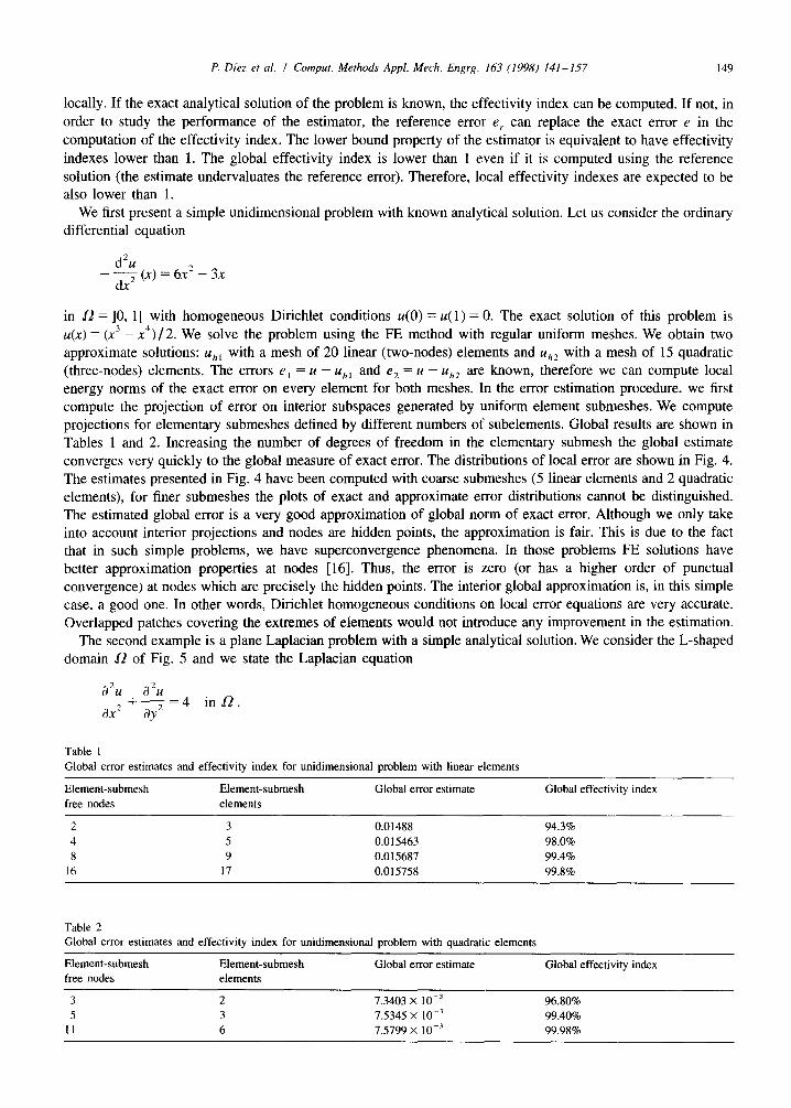
We first present a simple unidimensional problem with known analytical solution. Let us consider the ordinary

differential equation

- 2 (x) = 6~’ - 3x

in 0 = IO, 1[ with homogeneous Dirichlet conditions u(0) = u( 1) = 0. The exact solution of this problem is

u(x) = (x3 - x4) /2. We solve the problem using the FE method with regular uniform meshes. We obtain two

approximate solutions: uhl with a mesh of 20 linear (two-nodes) elements and u,,* with a mesh of 15 quadratic

(three-nodes) elements. The errors e, = u - uh, and e2 = u - uh2 are known, therefore we can compute local

energy norms of the exact error on every element for both meshes. In the error estimation procedure, we first

compute the projection of error on interior subspaces generated by uniform element submeshes. We compute

projections for elementary submeshes defined by different numbers of subelements. Global results are shown in

Tables 1 and 2. Increasing the number of degrees of freedom in the elementary submesh the global estimate

converges very quickly to the global measure of exact error. The distributions of local error are shown in Fig. 4.

The estimates presented in Fig. 4 have been computed with coarse submeshes (5 linear elements and 2 quadratic

elements), for finer submeshes the plots of exact and approximate error distributions cannot be distinguished.

The estimated global error is a very good approximation of global norm of exact error. Although we only take

into account interior projections and nodes are hidden points, the approximation is fair. This is due to the fact that in such simple problems, we have superconvergence phenomena. In those problems FE solutions have

better approximation properties at nodes [16]. Thus, the error is zero (or has a higher order of punctual

convergence) at nodes which are precisely the hidden points. The interior global approximation is, in this simple

case, a good one. In other words, Dirichlet homogeneous conditions on local error equations are very accurate.

Overlapped patches covering the extremes of elements would not introduce any improvement in the estimation.

The second example is a plane Laplacian problem with a simple analytical solution. We consider the L-shaped

domain R of Fig. 5 and we state the Laplacian equation

2 2

$+$=4 in R.

Table 1

Global error estimates and effectivity index for unidimensional problem with linear elements

Element-submesh

free nodes

Element-submesh

elements

Global error estimate Global effectivity index

2 3 0.01488 94.3%

4 5 0.015463 98.0%

8 9 0.015687 99.4%

16 17 0.015758 99.8%

Table 2

Global error estimates and effectivity index for unidimensional problem with quadratic elements

Element-submesh Element-submesh Global error estimate Global effectivity index free nodes elements

3 2 7.3403 x 1o-3 96.80%

5 3 7.5345 x lo-3 99.40%

11 6 7.5799 x lo-’ 99.98%

P. Diez et al. / Comput. Methods Appl. Mech. Engrg. 163 (1998) 141-157

__

#-

I __J

0.0 0.1 0.2 0.3 0.4 0.5 0.6 0.7 0.8 0.9 1.0 - 0.0 0.1 0.2 0.3 0.4 0.5 0.6 0.7 0.8 0.9 1.0

X X

Fig. 4. Distribution of error measures, exact error (solid line) and estimated error (dashed line) for linear elements (left) and quadratic

elements (right).

We give Dirichlet boundary conditions on the whole boundary of L2 such that we get the analytical exact

solution u(x, y) = x2 + y*. The approximate solution uh is computed using the unstructured quadrilateral mesh

shown in Fig. 5.

For this problem, error estimation is performed using both nodal and edge-patch approaches. Tables 3 and 4

show the evolution of global effectivity index with the number of elements in the element submesh for both

0.80 1.1 1.4 1.7 2.0 2.3 2.6 2.9 3.2 3.5 3.8 4.1 4.4 4.7

Fig. 5. Distribution of the exact error.


Table 3

Global error estimates and effectivity index for bidimensional Laplacian problem with four-noded quadrilateral elements and nodal patch

submeshes

Element-submesh

free nodes

Element-submesh

elements


9 16 0.24759 91.9%

2.5 36 0.25435 ‘34.4%

49 64 0.25670 95.3%

81 100 0.25780 95.7%

361 400 0.25934 97.5%

Table 4

Global error estimates and effectivity index for bidimensional Laplacian problem with four-noded quadrilateral elements and side patch

submeshes

Element-submesh

free nodes

Element-submesh

elements


Y 12 0.2338 1 86.8%

41 48 0.24315 90.2%

177 92 0.24691 91.6%

node-patch and edge-patch approaches. As we can see in Tables 3 and 4, in this case, the nodal-patch approach

presents slightly better results. Anyway, in both cases the estimation fits the shape of the distribution of the local

error. In fact, Fig. 5 shows the exact error distribution over the domain. Notice the similarity with Fig. 6 where

the estimated error is presented. The represented estimation corresponds to a nodal-patch approach with

elementary submeshes of 16 elements. As a measure of the quality of the estimator we also look at local

0.80 1.1 1.4 1.7 2.0 2.3 2.6 2.9 3.2 3.5 3.8 4.1 4.4 4.7

Fig. 6. Distribution of the estimated error.

1.52 P. Diez et al. I Comput. Methods Appl. Mech. Engrg. 163 (1998) 141-157

Effectivity index histogram

5(z

tw

effectivity index

Fig. 7. Histogram representing the occurrences of the values of local effectivity index for the Laplacian problem (represented for the

nodal-patch estimator and the elementary submesh of 16 elements).

effectivity indexes. The histogram representing the occurrences of the values of local effectivity index (Fig, 7)

shows the distribution of local underestimation and demonstrates that the spatial distribution of the local

effectivity index is quite uniform (the values are concentrated between 0.83 and 0.95). So, the equality of the estimation is roughly the same in the whole domain. This is very important if the estimator is used in an

82.

83.

84.

85.

86.

87.

88.

89.

90.

91.

92.

93.

94.

95.

Fig. 8. Distribution of the local effectivity index.


0.0

3.0

6.0

9.0

12.

15.

18.

21.

24.

27.

30.

33.

36.

39.

adaptive procedure because the mesh optimality criteria are based on the uniform spatial distribution of the

error. Fig. 8 shows the spatial distribution of the effectivity index. Notice that, although the estimation is more

accurate in the interior of the domain, on the boundary the effectivity index is over 0.92.

This example shows that the estimator has a good behavior even in the elements near the Dirichlet boundary.

Usually, standard error estimators present problems near the boundaries [2].

The third example is a plane elastic mechanical problem (in plane strain hypothesis). Displacements of a

gravity dam under water pressure and concrete and rock weight loads are computed using FE. We prescribe

displacements along the boundary representing the edge of the concerned ground domain. Reference error distribution and estimated error distribution are shown in Figs. 9 and 10. The error

0.0

3 *O :&?,,

:B 6.0

9.0

12.

15.

18.

I 21.

I 24.

I 27.

I 30.

I 33.

1 36.

I 39.

Fig. 10. Distribution of the estimated error.

154 P. Diez et al. I Comput. Methods Appl. Mech. Engrg. I63 (1998) 141-157

0.0

3.0

6.0 _., FL @: P.i 9.0

12.0

15.0

18.0

II 21.0

I 24.0

1 27.0

I 30.0

1 33.0

I 36.0

I 39.0

Fig. 11. Distribution of the Zienkiewicz-Zhu estimated error.

distribution obtained with the Zienkiewicz-Zhu estimator described in [3] is shown in Fig. 11. Fig. 12 shows

histograms of local values of effectivity index for the presented estimator and for the Zienkiewicz-Zhu

estimator described in [3]. The values of the effectivity index associated with the presented estimator are

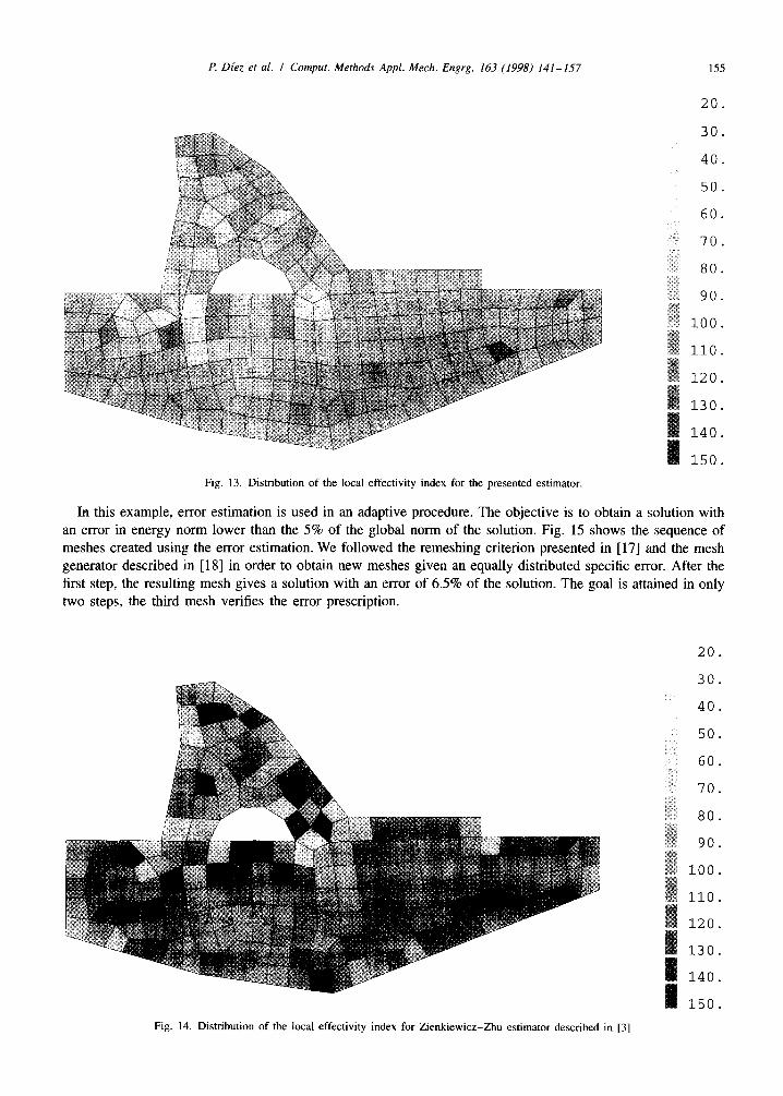
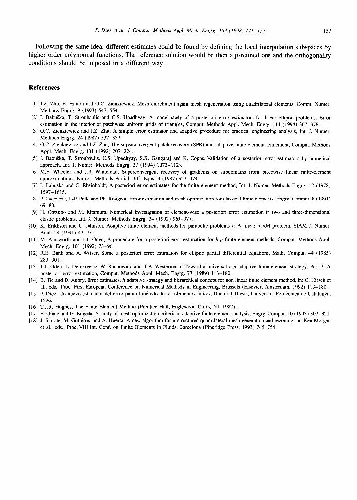
concentrated in a narrower band. A uniform bias and a little dispersion in this histogram means that the quality of the estimation is uniform and, therefore, the estimator is well suited to an adaptive procedure. Figs. 13 and 14

represent the distributions of the local effectivity index for the presented estimator and the Zienkiewicz-Zhu

estimator, respectively. Notice that spatial distribution of the local effectivity index for the presented estimator is

more uniform.

Effectivity index histogram

Fig. 12. Histogram representing the occurrences of the values of local effectivity index for the mechanical problem for both the presented

estimator (solid line) and the Zienkiewicz-Zhu estimator described in [3] (dashed line).

P. Diez et al. I Comput. Methods Appl. Mech. Emgrg. 163 (1998) 141-157 15.5

20.

30.

40.

50.

60.

70.

80.

90. :?C; $1. 1OO*

110.

120.

130.

140.

150.

Fig. 13. Distribution of the local effectivity index for the presented estimator.

In this example, error estimation is used in an adaptive procedure. The objective is to obtain a solution with

an error in energy norm lower than the 5% of the global norm of the solution. Fig. 15 shows the sequence of

meshes created using the error estimation. We followed the remeshing criterion presented in [17] and the mesh

generator described in [ 181 in order to obtain new meshes given an equally distributed specific error. After the

first step, the resulting mesh gives a solution with an error of 6.5% of the solution. The goal is attained in only

two steps, the third mesh verifies the error prescription.

20.

30.

40.

50.

60.

70.

80. &; ‘@

:$ 90.

6% 100.

110.

120.

130.

140.

150.

Fig. 14. Distribution of the local effectivity index for Zienkiewicz-Zhu estimator described in [3]


Fig. IS. Sequence of refined meshes leading to the optimal mesh giving 5% of relative error.

7. Conclusions

The methodology introduced in this paper provides a new approach to error estimation in FE analysis.

The presented lower bound estimator has a good performance approximating both the global value and the

shape of the error. Although it is a residual estimator, it does not need to approximate boundary conditions for

local problems. Therefore it is not necessary to compute flux jump cross the edges of each element and the error introduced by flux splitting techniques is avoided. One of the main disadvantages of the residual estimators is

then precluded. Moreover, the estimator is defined elementwise and it can be applied in meshes combining elements of

different shapes. The reference solution is approximated by solving local problems subject to homogeneous Dirichlet boundary conditions. Therefore standard routines of FE codes can be used to build up each local

problem. Consequently, the estimator is easily integrated in existing codes. Adaptive procedures using this estimator present fast convergence to optimal meshes given a specified

relative error. Further studies about the quality and the robustness of the estimator under strong regularity conditions can be

performed following the method described in [2] and [S].


Following the same idea, different estimates could be found by defining the local interpolation subspaces by higher order polynomial functions. The reference solution would be then a p-refined one and the orthogonality conditions should be imposed in a different way.

References

[l] J.Z. Zhu, E. Hinton and O.C. Zienkiewicz, Mesh enrichment again mesh regeneration using quadrilateral elements, Comm. Numer.

Methods Engrg. 9 (1993) 547-554.

[2] I. BabuSka, T. Strouboulis and C.S. Upadhyay, A model study of a posteriori error estimators for linear elliptic problems. Error

estimation in the interior of patchwise uniform grids of triangles, Comput. Methods Appl. Mech. Engrg. 114 (1994) 307-378.

[3] O.C. Zienkiewicz and J.Z. Zhu, A simple error estimator and adaptive procedure for practical engineering analysis, Int. J. Numer.

Methods Engrg. 24 (1987) 337-357.

[4] O.C. Zienkiewicz and J.Z. Zhu, The superconvergent patch recovery (SPR) and adaptive finite element refinement, Comput. Methods

Appl. Mech. Engrg. 101 (1992) 207-224.

[5] I. BabuBka, T. Strouboulis, C.S. Upadhyay, S.K. Gangaraj and K. Copps, Validation of a posteriori error estimators by numerical

approach, Int. J. Numer. Methods Engrg. 37 (1994) 1073-1123.

[6] M.F. Wheeler and J.R. Whiteman, Superconvergent recovery of gradients on subdomains from piecewise linear finite-element

approximations, Numer. Methods Partial Diff. Eqns. 3 (1987) 357-374.

[7] I. BabuSka and C. Rheinboldt, A-posteriori error estimates for the finite element method, Int. J. Numer. Methods Engrg. 12 (1978)

1597-1615.

[8] P. Lade&e, J.-P Pelle and Ph. Rougeot, Error estimation and mesh optimization for classical finite elements, Engrg. Comput. 8 (1991)

69-80.

[9] H. Ohtsubo and M. Kitamura, Numerical investigation of element-wise a posteriori error estimation in two and three-dimensional

elastic problems, Int. J. Numer. Methods Engrg. 34 (1992) 969-977.

[lo] K. Erikkson and C. Johnson, Adaptive finite element methods for parabolic problems I: A linear model problem, SIAM J. Numer.

Anal. 28 (1991) 43-77.

[ 1 l] M. Ainsworth and J.T. Oden, A procedure for a posteriori error estimation for h-p finite element methods, Comput. Methods Appl.

Mech. Engrg. 101 (1992) 73-96.

[12] R.E. Bank and A. Weiser, Some a postetiori error estimators for elliptic partial differential equations, Math. Comput. 44 (1985)

283-301.

[13] J.T. Oden, L. Demkowicz, W. Rachowicz and T.A. Westermann, Toward a universal h-p adaptive finite element strategy, Part 2. A

posteriori error estimation, Comput. Methods Appl. Mech. Engrg. 77 (1989) 113-180.

[14] B. Tie and D. Aubry, Error estimates, h adaptive strategy and hierarchical concept for non linear finite element method, in: C. Hirsch et

al., eds., Proc. First European Conference on Numerical Methods in Engineering, Brussels (Elsevier, Amsterdam, 1992) 113-180.

[ 151 P. Diez, Un nuevo estimador de1 error para el metodo de 10s elementos finitos, Doctoral Thesis, Universitat Politecnica de Catalunya,

1996.

[16] T.J.R. Hughes, The Finite Element Method (Prentice Hall, Englewood Cliffs, NJ, 1987).

[ 171 E. Oiiate and G. Bugeda, A study of mesh optimization criteria in adaptive finite element analysis, Engrg. Comput. 10 (1993) 307-321.

[ 181 J. Sat-rate, M. Gutiirrez and A. Huerta, A new algorithm for unstructured quadrilateral mesh generation and rezoning, in: Ken Morgan

et al., eds., Proc. VIII Int. Conf. on Finite Elements in Fluids, Barcelona (Pineridge Press, 1993) 745-754.

Documents

A posteriori error estimation for standard finite element analysis