A Power System Reliability Evaluation Technique and Education Tool for Wind

Energy Integration

by

Anubhav Sinha

A Thesis Presented in Partial Fulfillment

of the Requirements for the Degree

Master of Science

Approved February 2012 by the

Graduate Supervisory Committee:

Gerald Heydt, Co-Chair

Vijay Vittal, Co-Chair

Raja Ayyanar

George Karady

ARIZONA STATE UNIVERSITY

May 2012

All rights reserved

INFORMATION TO ALL USERSThe quality of this reproduction is dependent on the quality of the copy submitted.

In the unlikely event that the author did not send a complete manuscriptand there are missing pages, these will be noted. Also, if material had to be removed,

a note will indicate the deletion.

All rights reserved. This edition of the work is protected againstunauthorized copying under Title 17, United States Code.

ProQuest LLC.789 East Eisenhower Parkway

P.O. Box 1346Ann Arbor, MI 48106 - 1346

UMI 1508104Copyright 2012 by ProQuest LLC.

UMI Number: 1508104

i

ABSTRACT

This thesis is focused on the study of wind energy integration and is divid-

ed into two segments. The first part of the thesis deals with developing a reliabil-

ity evaluation technique for a wind integrated power system. A multiple-partial

outage model is utilized to accurately calculate the wind generation availability. A

methodology is presented to estimate the outage probability of wind generators

while incorporating their reduced power output levels at low wind speeds. Subse-

quently, power system reliability is assessed by calculating the loss of load proba-

bility (LOLP) and the effect of wind integration on the overall system is analyzed.

Actual generation and load data of the Texas power system in 2008 are

used to construct a test case. To demonstrate the robustness of the method, relia-

bility studies have been conducted for a fairly constant as well as for a largely

varying wind generation profile. Further, the case of increased wind generation

penetration level has been simulated and comments made about the usability of

the proposed method to aid in power system planning in scenarios of future ex-

pansion of wind energy infrastructure.

The second part of this thesis explains the development of a graphic user

interface (GUI) to demonstrate the operation of a grid connected doubly fed in-

duction generator (DFIG). The theory of DFIG and its back-to-back power con-

verter is described. The GUI illustrates the power flow, behavior of the electrical

circuit and the maximum power point tracking of the machine for a variable wind

speed input provided by the user. The tool, although developed on MATLAB

software platform, has been constructed to work as a standalone application on

ii

Windows operating system based computer and enables even the non-engineering

students to access it.

Results of both the segments of the thesis are discussed. Remarks are pre-

sented about the validity of the reliability technique and GUI interface for variable

wind speed conditions. Improvements have been suggested to enable the use of

the reliability technique for a more elaborate system. Recommendations have

been made about expanding the features of the GUI tool and to use it to promote

educational interest about renewable power engineering.

iii

ACKNOWLEDGEMENT

I would like to thank Arizona State University and the US Department of

Energy (grant award number: DE-EE0000535) for their support for this project. I

owe a deep gratitude to Dr. Gerald Heydt, Dr. Vijay Vittal and Dr. Raja Ayyanar

for their precious guidance and motivation in course of research and also while

finalizing this thesis. Their recommendations and suggestions have been extreme-

ly helpful and would serve as invaluable learning for me even beyond this project.

I would like to thank my committee, Dr. Gerald Heydt, Dr. Vijay Vittal, Dr.

George Karady and Dr. Raja Ayyanar for their time and assistance.

Special thanks to my family, friends and colleagues for providing support

and appreciation of my work and for rendering advice whenever it was needed the

most.

iv

TABLE OF CONTENTS

Page

LIST OF TABLES.……………………………………………………………..viii

LIST OF FIGURES……………………………………………………………....ix

NOMENCLATURE……………………………………………………………..xii

CHAPTER

1 INTRODUCTION TO WIND ENERGY RELIABILITY AND WIND GEN-

ERATION CONFIGURATIONS…………………………………..…………1

1.1 Objectives………………………………………………………………....1

1.2 Motivation…………………………………………………………………2

1.2.1 Reliability studies for wind integrated power systems……………...2

1.2.2 A “hands on” educational tool for DFIG wind energy systems……..3

1.3 Literature survey: partial outage representation in conventional generation

system…..…………………………………………………………...…….4

1.4 Literature survey: impact of wind generation on LOLP…………………..6

1.5 Literature survey: wind generation configurations for wind turbines.........8

1.6 Organization of thesis…………………………………………………....10

2 THEORY AND ANALYSIS OF POWER SYSTEM RELIABILITY STUD-

IES…………………………………………………………………...….........12

2.1 System reliability and its measurement…………………………….........12

v

CHAPTER Page

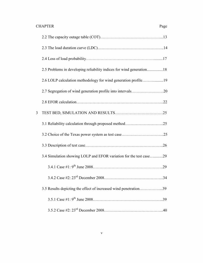
2.2 The capacity outage table (COT)………………………………………...13

2.3 The load duration curve (LDC)…………………………………………..14

2.4 Loss of load probability…………………………………………….........17

2.5 Problems in developing reliability indices for wind generation................18

2.6 LOLP calculation methodology for wind generation profile……….........19

2.7 Segregation of wind generation profile into intervals……………………20

2.8 EFOR calculation………………………………………………………...22

3 TEST BED, SIMULATION AND RESULTS………………………………25

3.1 Reliability calculation through proposed method………………………..25

3.2 Choice of the Texas power system as test case…………………………..25

3.3 Description of test case…………………………………………………..26

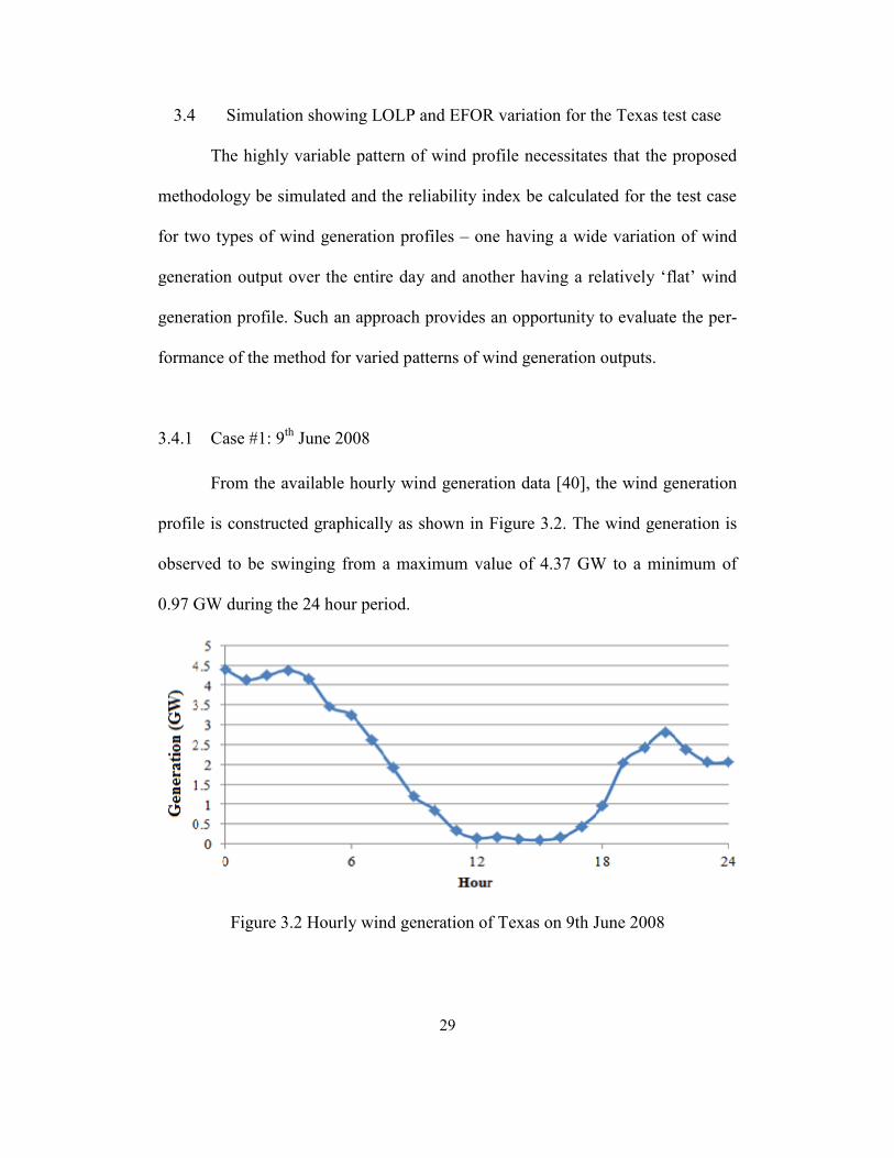
3.4 Simulation showing LOLP and EFOR variation for the test case….........29

3.4.1 Case #1: 9th

June 2008……………………………………………..29

3.4.2 Case #2: 23rd

December 2008……………………………………...34

3.5 Results depicting the effect of increased wind penetration……………...39

3.5.1 Case #1: 9th

June 2008……………………………………………..39

3.5.2 Case #2: 23rd

December 2008……………………………………...40

vi

CHAPTER Page

4 THEORY OF WIND GENERATION TECHNOLOGIES AND THE DFIG

POWER CONVERTER TOPOLOGY……………………………………....42

4.1 Overview: wind turbine configurations…………………………….........42

4.2 The doubly fed induction generators……………………………….........45

4.2.1 Power flow in a DFIG machine……………………………………45

4.2.2 The rotor side converter……………………………………………49

4.2.3 The grid side converter…………………………………………….51

4.2.4 Equivalent circuit for a DFIG……………………………………...51

4.2.5 Phasor diagram of a DFIG machine………………………………..53

5 CONSTRUCTION OF A GRAPHICAL USER INTERFACE FOR THE

DFIG GENERATION SYSTEM……………………………………….........55

5.1 Choice of MATLAB for GUI construction……………………………...55

5.2 Features of the GUI for simulation of a DFIG system…………………...56

5.2.1 The power flow interface…………………………………………..57

5.2.2 The equivalent circuit interface……………………………………59

5.2.3 The phasor diagram interface………………………………………60

5.2.4 Maximum power point tracking interface………………………….62

vii

CHAPTER Page

6 CONCLUSIONS AND RECOMMENDATIONS…………………………..65

6.1 Reliability assessment technique………………………………………...65

6.2 GUI construction for a DFIG system……………………………….........66

REFERENCES…………………………………………………………………..67

APPENDIX

A MATLAB CODE FOR RELIABILITY STUDY IMPLEMENTATION ON

TEXAS POWER SYSTEM…………………………….…………................72

B MATLAB CODE FOR THE DFIG OPERATION GUI……………..……...93

C INSTALLATION INSTRUCTIONS FOR STAND ALONE GUI………...129

viii

LIST OF TABLES

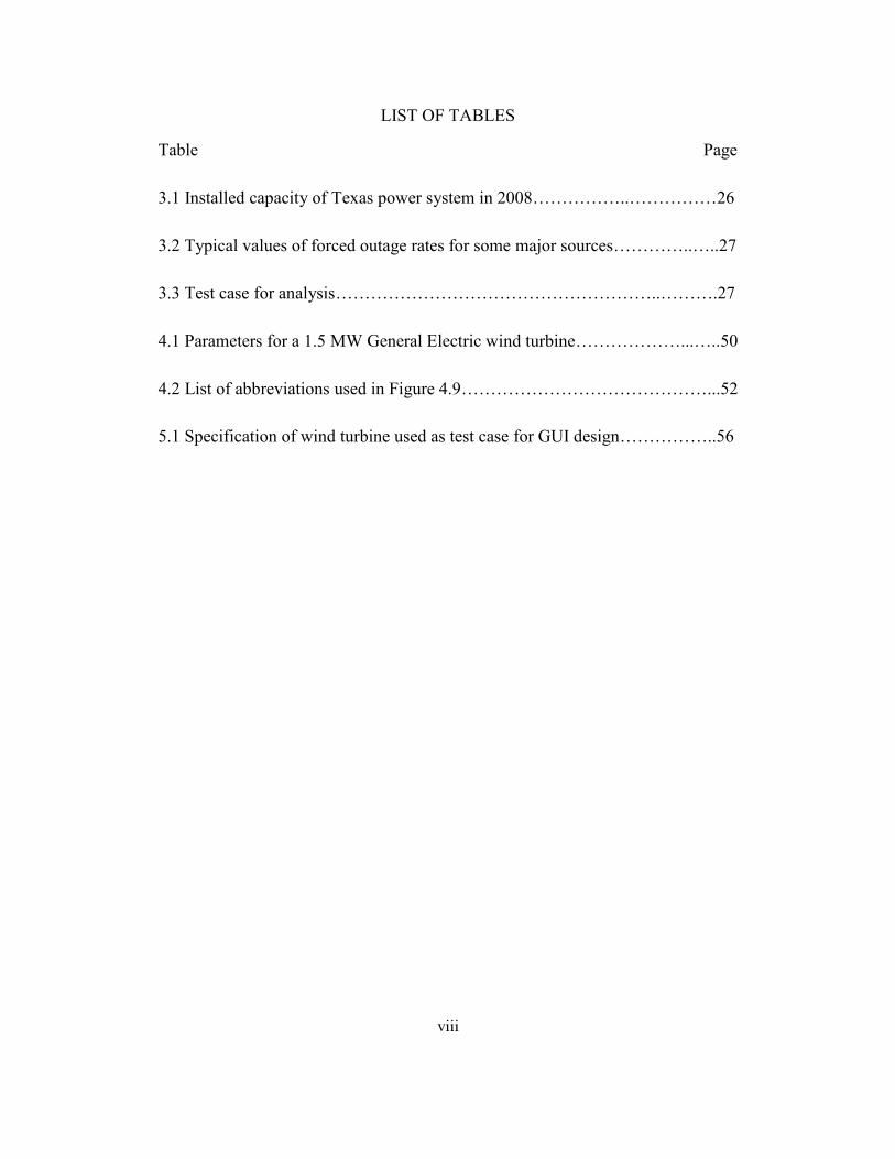
Table Page

3.1 Installed capacity of Texas power system in 2008……………..……………26

3.2 Typical values of forced outage rates for some major sources…………..…..27

3.3 Test case for analysis………………………………………………..……….27

4.1 Parameters for a 1.5 MW General Electric wind turbine………………...…..50

4.2 List of abbreviations used in Figure 4.9……………………………………...52

5.1 Specification of wind turbine used as test case for GUI design……………..56

ix

LIST OF FIGURES

Figure Page

1.1 Motivation and approach for the thesis………………………………………..2

2.1 Typical capacity outage table………………………………………………...14

2.2 Example of a load curve……………………………………………………..15

2.3 Load duration curve derived from Figure 2.2………………………………..15

2.4 Load duration curve for a high load factor…………………………………..16

2.5 Load duration curve for a low load factor…………………………………...16

2.6 Wind generation profile of Texas in June 2008……………………………...20

2.7 Derivation of additional data points by using cubic splines…………………22

2.8 Flowchart depicting proposed methodology of LOLP calculation…………..24

3.1 Load duration curve for load in Texas in year 2008…………………………27

3.2 Hourly wind generation of Texas on 9th

June 2008………………………….29

3.3 Individual generation profile of wind generators in test case………………..30

3.4 Derivation of additional data points by implementing cubic spline for 72 inte-

vals……………………..…………………………………………...………..31

3.5 Variation of LOLP with change in number of intervals……………………..33

3.6 Variation of EFOR with change in number of intervals……………………..33

3.7 Hourly wind generation of Texas on 23rd

December 2008…………………..35

x

Figure Page

3.8 Individual generation profile of wind generators in test case #2…………….35

3.9 Derivation of additional data points by implementing cubic spline for 72 inte-

vals..……………………………………………………………………...…..36

3.10 Variation of LOLP with change in number of intervals for case #2………..37

3.11 Variation of EFOR with change in number of intervals for case #2……….38

3.12 LOLP variation with change in wind penetration level for case #1………..39

3.13 EFOR variation with change in wind penetration level for case #1………..40

3.14 LOLP variation with change in wind penetration level for case #2………..40

3.15 EFOR variation with change in wind penetration level for case #2………..41

4.1 Type 1 wind turbine configuration…………………………………………..43

4.2 Type 2 wind turbine configuration…………………………………………..43

4.3 Type 3 wind turbine configuration…………………………………………..44

4.4 Type 4 wind turbine configuration…………………………………………..44

4.5 Power flow in a DFIG based configuration (Type 3)………………………..45

4.6 Power flow in a DFIG machine in subsynchronous mode…………………..48

4.7 Power flow in a DFIG machine in supersynchronous mode………………...48

4.8 Turbine tracking characteristics……………………………………………...51

4.9 Equivalent circuit of a DFIG machine……………………………………….52

xi

Figure Page

4.10 Phasor diagram of a DFIG machine for a unity power factor………………54

4.11 Phasor diagram of a DFIG machine for a lagging power factor……………54

5.1 Power flow GUI showing subsynchronous operation……………………….58

5.2 Power flow GUI showing supersynchronous operation……………………..58

5.3 DFIG equivalent circuit GUI interface for unity power factor operation at

wind speed 7 m/s……………………..………………………………………59

5.4 DFIG equivalent circuit GUI interface for unity power factor operation at

wind speed 10 m/s………………..…………………………………………..60

5.5 Wind speed 14 m/s and unity power factor………………………………….61

5.6 Wind speed 14 m/s and power factor angle -35 degrees…………………….61

5.7 Wind speed 14 m/s and power factor angle 35 degrees……………………...62

5.8 Maximum power point tracking GUI at wind speed 6 m/s…………………..63

5.9 Maximum power point tracking GUI at wind speed 9 m/s………………......63

5.10 Maximum power point tracking GUI at wind speed 12.5 m/s……………...64

xii

NOMENCLATURE

A Area swept by wind turbine blades

ARMA Autoregressive moving average

ci Constants used to calculate wind turbine power coefficient

Cp Wind turbine power coefficient

CDF Cumulative probability density

COT Capacity outage table

DF Derating factor

DFIG Doubly fed induction generator

E Generator internal EMF

EFOR Equivalent forced outage rate

EFORd Equivalent demand forced outage rate

EMF Electro motive force

ERCOT Electric Reliability Council of Texas

f0 Probability of full capacity outage

FOH Forced outage hours

FOR Forced outage rate

GE General Electric Co.

GUI Graphic user interface

Im DFIG magnetizing current

Ir’ DFIG rotor current reflected to primary

Is DFIG stator current

Llr Rotor leakage inductance

Lls Stator leakage inductance

Lm Magnetizing inductance

LDC Load duration curve

LOLE Loss of load expectation

LOLP Loss of load probability

Pgap Power transferred trough air gap

Ploss_rotor Power loss in the rotor circuit

Ploss_stator Power loss in the stator circuit

Pm Power input into rotor from wind turbine

Pm_pu Per unit power input into rotor from turbine

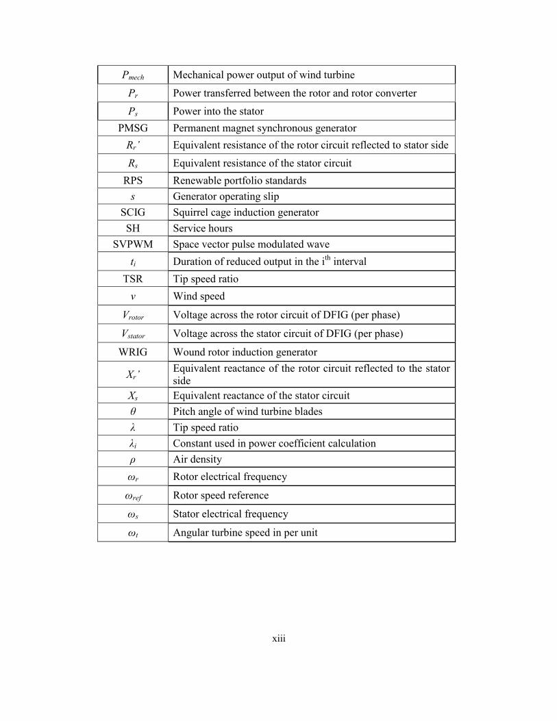
xiii

Pmech Mechanical power output of wind turbine

Pr Power transferred between the rotor and rotor converter

Ps Power into the stator

PMSG Permanent magnet synchronous generator

Rr’ Equivalent resistance of the rotor circuit reflected to stator side

Rs Equivalent resistance of the stator circuit

RPS Renewable portfolio standards

s Generator operating slip

SCIG Squirrel cage induction generator

SH Service hours

SVPWM Space vector pulse modulated wave

ti Duration of reduced output in the ith

interval

TSR Tip speed ratio

ν Wind speed

Vrotor Voltage across the rotor circuit of DFIG (per phase)

Vstator Voltage across the stator circuit of DFIG (per phase)

WRIG Wound rotor induction generator

Xr’ Equivalent reactance of the rotor circuit reflected to the stator

side

Xs Equivalent reactance of the stator circuit

θ Pitch angle of wind turbine blades

λ Tip speed ratio

λi Constant used in power coefficient calculation

ρ Air density

ωr Rotor electrical frequency

ωref Rotor speed reference

ωs Stator electrical frequency

ωt Angular turbine speed in per unit

1

CHAPTER 1

INTRODUCTION TO WIND ENERGY RELIABILITY AND WIND GENER-

ATION CONFIGURATIONS

1.1 Objectives

Reliability analysis in power system planning and power electronics is the

key driving force to enable an enhanced wind generation penetration in the future.

To realistically visualize the effect of increased wind penetration and to estimate

the extent of penetration possible, accurate power system reliability analysis tech-

niques are necessary. Additionally, to realize a targeted level of wind energy pen-

etration, efficient power electronics technology is instrumental for large scale

wind integration. A further objective of this thesis is to provide an educational

tool as a framework and motivating element for students who might make their

careers in the electric energy area. The main objectives of this thesis are to evalu-

ate the role of reliability analysis and power electronics and to provide an educa-

tional tool relating to wind energy by:

Developing an accurate reliability representation for wind integrated pow-

er systems and to enable power systems planning.

Developing an educational tool to promote an understanding of contempo-

rary wind generator technology including power electronics.

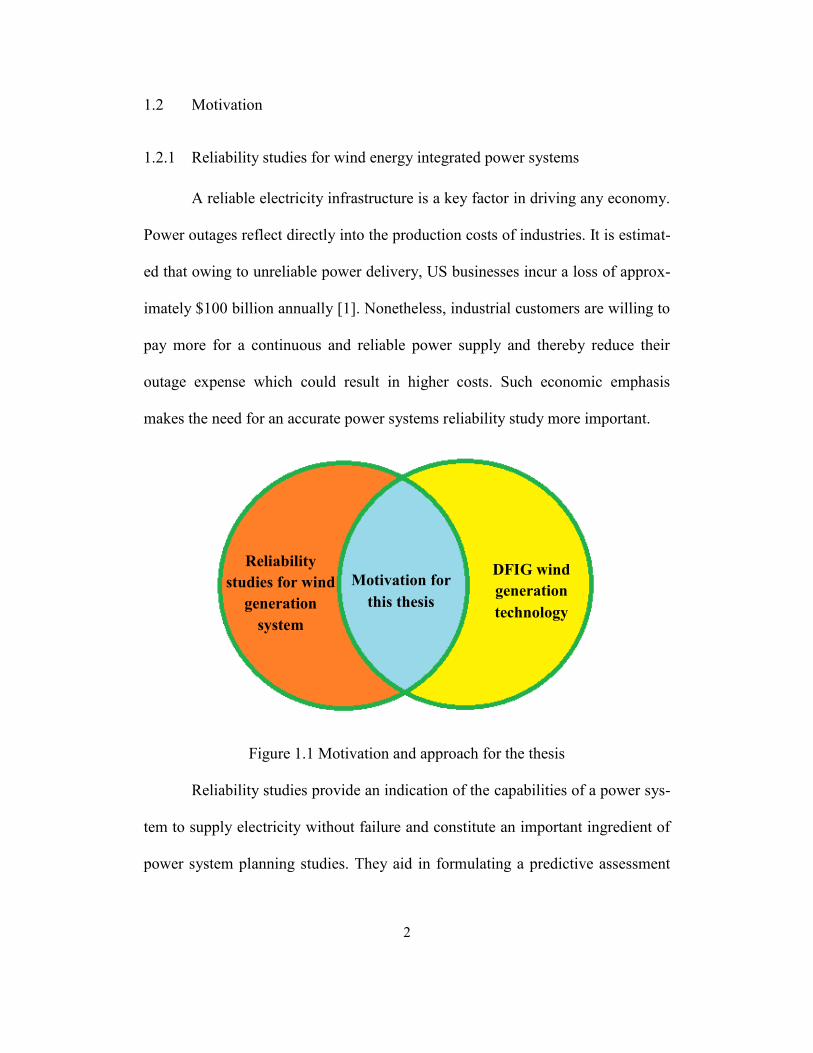
Figure 1.1 pictorially describes the motivation and approach of this thesis.

2

1.2 Motivation

1.2.1 Reliability studies for wind energy integrated power systems

A reliable electricity infrastructure is a key factor in driving any economy.

Power outages reflect directly into the production costs of industries. It is estimat-

ed that owing to unreliable power delivery, US businesses incur a loss of approx-

imately $100 billion annually [1]. Nonetheless, industrial customers are willing to

pay more for a continuous and reliable power supply and thereby reduce their

outage expense which could result in higher costs. Such economic emphasis

makes the need for an accurate power systems reliability study more important.

Figure 1.1 Motivation and approach for the thesis

Reliability studies provide an indication of the capabilities of a power sys-

tem to supply electricity without failure and constitute an important ingredient of

power system planning studies. They aid in formulating a predictive assessment

Motivation for

this thesis

DFIG wind

generation

technology

Reliability

studies for wind

generation

system

3

of customer outage cost and thus help towards designing a ‘fail-safe’ infrastruc-

ture that meets the desired level of expectancy of power delivery [2].

While conducting reliability studies for any typical power system, calcula-

tion of an index such as the loss of load probability (LOLP) requires three ingre-

dients:

An accurate model of the generating unit availability,

An estimate of the generating unit outages and

Information about the behavior of the load.

Although all of these quantities are subject to variation, they are fairly predictable

for analysis of conventional generation systems. However, such calculations be-

come inaccurate if there is a significant share of variable sources such as wind

generators.

In recent decades, there has been an increased penetration of renewable

energy (especially wind energy) into the electrical power system. For instance, in

the US, the installed wind generation capacity rose from 6456 MW (0.67% of to-

tal installed generation) in 2004 [3] to 43461 MW (4.18% of installed generation)

in 2011 [4], [5]. Further, with US states establishing renewable portfolio standards

(RPS) goals for the decade, steep increase in wind generation installation is ex-

pected [6].

This thesis discusses the challenges of using the existing reliability study

model (applicable to conventional generation) for the wind energy systems and

proposes a methodology to include the effect of partial power outputs of wind

4

generators (e.g., during low wind conditions) while still using the existing reliabil-

ity indices to measure system reliability. The performance of the proposed meth-

odology is further analyzed by implementing it on the Texas power system and

observing its response to a rise in the wind generation penetration level from 5 to

10 % of the total installed generation capacity.

1.2.2 A “hands on” educational tool for DFIG wind energy systems

A significant integration of wind energy in the future would require a ded-

icated power engineering workforce having an in-depth knowledge of wind gen-

eration technology. Planning for the future, a focused approach has been devised

in this project which was funded by the U.S Department of Energy [7]. This pro-

ject aims to educate high school and undergraduate electrical engineering students

and motivate them to pursue a career in the field of wind power engineering.

This thesis, which is a part of the above mentioned project, contributes to

the initiative by developing a simplified graphic user interface (GUI) that demon-

strates the operation of a doubly fed induction generator (DFIG) based wind gen-

eration systems. The GUI is constructed using the MATLAB software.

1.3 Literature survey: partial outage representation for conventional generation

For a conventional generation system having a static capacity, a binary

representation may be employed to denote the availability of a generating unit

where the random failures of generating units is expressed in terms of forced out-

age rate (FOR). However, in such a representation, neglecting partial outages or

5

defining them as full outages leads to inaccurate results for reliability study calcu-

lations - especially for generating units with large size or having a variable pattern

of generation.

Extensive literature is available that propose techniques of representing

the availability of a partially loaded generation unit as well as its outage probabil-

ity. By utilizing the Markov approach, reference [8] develops a single partial out-

age model to calculate transient outage probability. In this context, the Markov

approach relies on the analysis of system states and transitions between system

states with the assumption that transition probabilities are fixed. The author cate-

gorizes the service of a generator into three states of operation namely, a fully op-

erational state, a derated state and a complete outage state and discusses the

treatment of derating in probability calculations. The paper proceeds to evaluate

the effect of the method on LOLP calculations.

In reference [9], a multiple-partial outage model is used for static capacity

planning studies. Partial outages over a time interval create a number of capacity

levels. The derated levels are grouped into some selected capacity levels which

are defined on the basis of the probability of occurrence of the outage event. The

paper expresses the outage probability in terms of an equivalent forced outage rate

(EFOR). The effect of EFOR representation on calculation accuracy and econom-

ic benefits is analyzed for a selected test case.

Reference [10] discusses the improvement in reliability study calculation

by using a multi-state representation of generation unit availability (for cases of

partial outages) as compared to modeling the outage probability as an EFOR.

6

Reference [11] evaluates system reliability by calculating LOLP for a

power system with partially loaded machines governed by economic dispatch al-

gorithms. A multi-state model is used to represent the partial commitment of gen-

erating units. The effect of load variation on partial loading of machines is incor-

porated by using a convolution technique to derive an equivalent load curve for

each committed unit on the basis of the available hourly load data.

1.4 Literature survey: impact of wind generation on LOLP

LOLP is an index used to measure power system reliability. An elaborate

description of the classical LOLP calculation methodology for conventional gen-

eration system is discussed in reference [12]. Reference [13] demonstrates LOLP

calculation for a chosen power system test case and proceeds to compare its per-

formance as compared to the load-loss frequency and duration index.

Wind generation is variable and its higher penetration into power systems

leads to a fluctuating and inaccurate estimation of generation availability and out-

age probability formulation. Hence, LOLP calculation for wind energy integrated

power systems by use of methods described in references [12] and [13] would

lead to unreliable results.

Studies in recent times have proposed numerous models to derive genera-

tion availability for wind integrated systems. Reference [14] uses a Monte Carlo

method to simulate wind conditions and appropriately represent the generation

availability. The author takes into account the wind speed dynamics and imple-

ments an autoregressive moving average (ARMA) wind model [15] for analysis.

7

The use of a time series wind model is discussed in reference [16] which

computes the wind generator power output based on the hourly wind speeds. Such

analysis includes the chronological characteristics of the generated wind energy.

However, the method requires exhaustive wind data for the site under analysis.

Reference [17] employs a multi-state model of wind speed to calculate the

wind generation with the aid of power curves at various output states. This refer-

ence proceeds to construct the cumulative probability density function (CDF) of

each of the wind generators. The paper formulates an equivalent CDF of a wind

farm total output which is derived from the characteristics of the individual wind

generators on in the farm. Subsequently, LOLP is calculated for the system under

study and the effect of increased wind penetration is investigated. In a similar

study, the short-term impact of wind generation on LOLP is presented in refer-

ence [18]. It constructs an instantaneous multi-state model to characterize the

wind generation output.

Although there has been an intensive research for deriving a generation

availability model for wind integrated power systems, industry and academia

seem divided over an exact approach for estimating the probability of total out-

age. Reference [16] simulates reliability studies for a selected test bed by using

time series model. The author, however, does not derive any definite model for

calculating outage probability for the wind integrated system and simply uses a

fixed value of 0.05 for FOR and assumes that the units operate in binary states.

Reference [19] provides a list of the average values of equivalent demand forced

outage rate (EFORd) used by ISO New England for reliability analysis. The doc-

8

ument also illustrates the use of the values of EFORd of hydro generating units

for analysis of wind generating systems.

A more pragmatic approach is followed by reference [20] which models

the entire wind park as a single unit and devises an equivalent FOR to account for

wind uncertainty. The FOR is defined in terms of ‘interval numbers’ which indi-

cate a range of possible values the wind generators under study may assume. The

authors also propose the scope to expand the work by the use of fuzzy logic to

formulate outage uncertainty. This approach is taken in order to aid in a more in-

tuitive approach for decision making in the expansion planning process.

1.5 Literature survey: wind generation configurations for wind turbines

Before the advent of efficient power electronics technologies, the wind

turbine driven induction generators were directly connected to the electrical grid

through a mechanical gearbox. Popularly known as the ‘Danish Concept’ of inter-

connection [21] such a topology is a fixed speed turbine system. Although it is an

inexpensive technology, such turbines are incapable of accurately controlling the

power quality of injected power [22] or delivering optimum power transfer unless

the wind blows near its designed operational speed [23]. On the other hand, a var-

iable speed turbine uses power electronics converters to overcome most of such

issues. However, they are costlier in comparison to the fixed speed systems.

A variety of literature exists that aims at improving the performance of

fixed and variable speed turbines. Reference [24] discusses the influence of me-

chanical characteristics of turbine (such as the inertial constant) and grid parame-

9

ters (like the short circuit power) on the transient voltage stability of a fixed speed

wind turbine. The paper evaluates the response of the turbine for a simulated fault

condition. An application of power electronics to fixed speed systems is demon-

strated in reference [25] which discusses a method to improve the transient volt-

age stability of fixed speed turbines by installing a power converter next to the

induction generators. Reference [26] proposes a novel design for equipment that

improves the power quality of fixed speed generators by utilizing power electron-

ics converters to cancel harmonic content in the power output.

For variable speed systems, a number of configurations have been pro-

posed and implemented. The performance of a variable speed turbine topology is

evaluated in reference [27] where a cascaded rectifier and inverter combination is

connected between the grid and the wind generator. The paper implements a

unique algorithm to eliminate voltage and frequency fluctuation in the output. In

a different approach, reference [28] illustrates the implementation of a cascaded

multilevel converter for variable speed turbines by using multiple permanent

magnet synchronous generator (PMSG) drive configuration and highlights its

benefits.

Power quality enhancement of variable speed generator output by the use

of an AC-AC matrix converter is demonstrated in reference [29]. The author high-

lights the benefit of the configuration to attain a smoother speed control and an

increased efficiency as compared to the DC-link voltage source converter.

The dynamic response of a DFIG based turbine technology and its ability

to control the active and reactive power injection into grid by the use of a space

10

vector pulse wave modulated (SVPWM) converter is discussed in reference [30].

Reference [31] proposes a fault detection scheme for back-to-back converters in

DFIG-based wind generation system.

1.6 Organization of thesis

This thesis has been organized into six chapters. Chapter 1 discusses the

objective and motivation of the thesis. It also details a literature summary on top-

ics of partial outage representation of generation systems, wind integration impact

on power system reliability and different wind turbine configurations prevalent.

Chapter 2 outlines the theory and calculation methodology to evaluate

power system reliability. It explains the demerits of using the conventional relia-

bility technique for wind integrated power systems. It proceeds to propose a

methodology for computing the outage probability of the wind generators and the

overall reliability of wind connected systems.

The proposed technique is simulated on a realistic test case in Chapter 3.

The values of LOLP and outage probabilities of wind generators are calculated

and remarks are made to demonstrate an increase in reliability study accuracy by

using the new methodology. The case of an increased wind generation penetration

is also simulated and its effect on overall power system reliability is discussed.

Chapter 4 explains the theory of the prevalent wind turbine technologies.

The working of the grid connected DFIG machine is outlined and the operation

mechanism of the power converters is elaborated in detail. Equations related to

11

power flow equation and maximum power point tracking mechanism are also

elaborated upon.

Chapter 5 focuses on describing the construction of the GUI for the DFIG

system. It discusses the basis of choosing MATLAB as the software to construct

the GUI. It also illustrates the different components of the GUI and explains its

features.

Conclusions, recommendations and future scope of the presented work are

provided in Chapter 6. The appendices A and B contain the MATLAB code used

to develop the reliability model calculation for the test case and the GUI tool. Ap-

pendix C describes the instructions to install the standalone version of the GUI on

a Windows operating system based computer.

12

CHAPTER 2

THEORY AND ANALYSIS OF POWER SYSTEM RELIABILITY STUDIES

2.1 System reliability and its measurement

The ability of a device or system to perform a required function under

stated conditions for the desired period of time is termed as reliability [32]. A

myriad of system abnormalities such as protection component failures, control or

communication failures, accidents or operational errors make the power system

vulnerable. Loss of service of generating units has a significant effect on the per-

formance of utility systems as well as on the consumer and result in revenue loss-

es amounting to tens of millions of dollars [33]. This amount increases apprecia-

bly if partial outages are also accounted for in the cost analysis and accurately

represented. Therefore, to perceive the cost of unreliable operation of a power

system, indices have been formulated to accurately represent the service availabil-

ity.

Mathematically, reliability is the probability that a device would perform

its required function for a specified period of time under the stated operational

conditions. For conventional generators, the FOR serves as its reliability indicator

and is defined as,

)( FOHSH

FOHFOR

(2.1)

where, SH: service hours, FOH: forced outage hours. Neglecting partial outages

altogether or representing them as a full outage leads to an incorrect forced outage

13

rate. Therefore, a multistate derated model is used where the partial outage proba-

bility is weighted by the fraction of the capacity lost and added to the probability

of total outage [9]. The ‘weighted’ forced outage rate thus obtained is defined as

an EFOR.

On the basis of service availability data of each individual generating unit,

their outage probability (expressed in terms of FOR or EFOR) and the load profile

data, the overall reliability of the entire power system is usually assessed in terms

of the following reliability indicators [34]:

LOLP: It is the probability that generation will be insufficient to meet the

demand at some point over a specific time window.

Loss of load expectation (LOLE): It is a measure of how long the availa-

ble capacity is likely to fall short of demand. It is obtained by calculating

the probability of daily peak demand exceeding the available capacity for

each day and adding these probabilities for all days in a year.

LOLP, unlike LOLE, quantifies the extent to which supply fails to meet

demand. Of course, LOLE refers to the energy not served whereas LOLP is the

probability of failure to meet the load. This thesis uses LOLP to evaluate the sys-

tem reliability.

2.2 The capacity outage table (COT)

For a fixed capacity level, the COT is used to compute the probability for

which the total generation capacity is unavailable due to forced outages exceeding

a particular threshold [35]. Figure 2.1 depicts the layout of a COT. The first col-

14

umn of the table contains all the capacity states in ascending order of outage mag-

nitude. If the system contains identical units then binomial distribution can be

used to calculate the COT. The second column lists the corresponding probability

of outages for a particular capacity state.

Available generation capacity Probability of outage

Lists the combination of

possible capacity states

Lists the corresponding probabil-

ity for the capacity state to have

outage

Figure 2.1 Typical capacity outage table

For a system having a large number of machines, the COT is generated by

interpolation. With the aid of the load duration curve, the COT is used to calculate

the LOLP. Also the COT indicates the expected generation margin which is de-

fined as the difference between the available generation and the load.

2.3 The load duration curve (LDC)

The LDC depicts the relation between capacity utilization and the duration

for which a load is served. It is a load curve in which the demand data is arranged

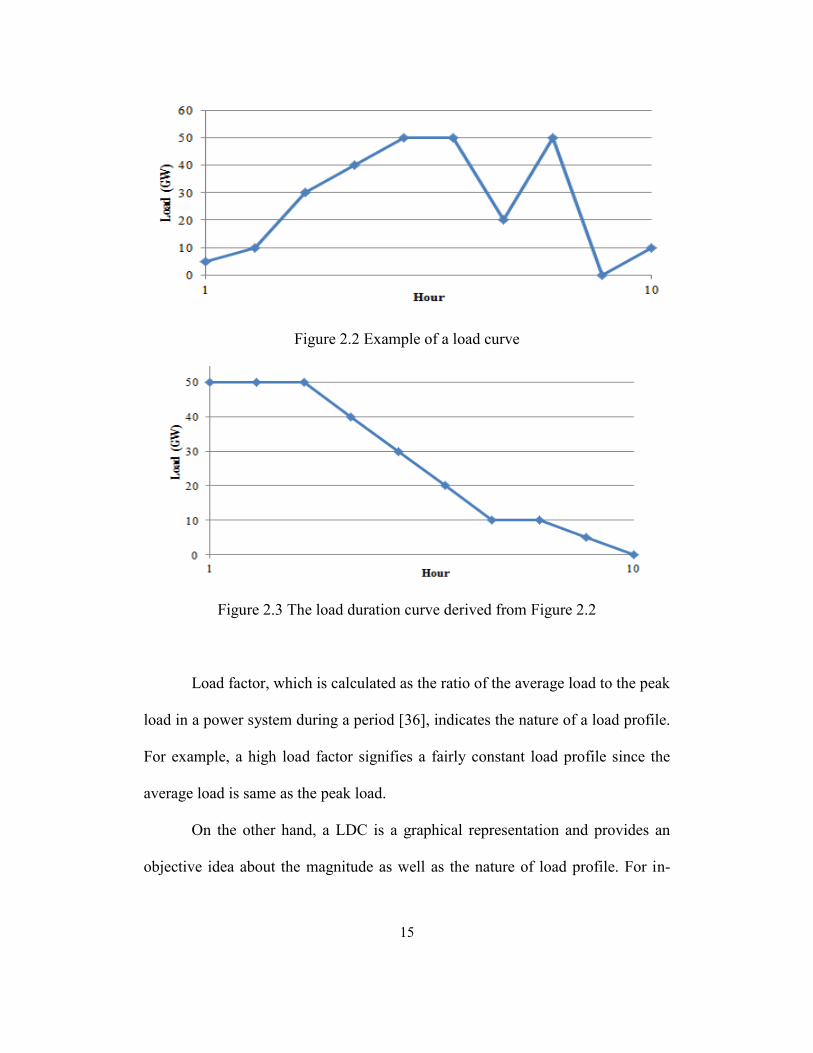
in descending order of magnitude. Figure 2.2 shows a load curve versus time

(showing load variation for 10 hours) and the LDC derived from it is shown in

Figure 2.3. Note that some LDCs as depicted in Fig. 2.3 are represented with the

abscissa and ordinate reversed.

15

Figure 2.2 Example of a load curve

Figure 2.3 The load duration curve derived from Figure 2.2

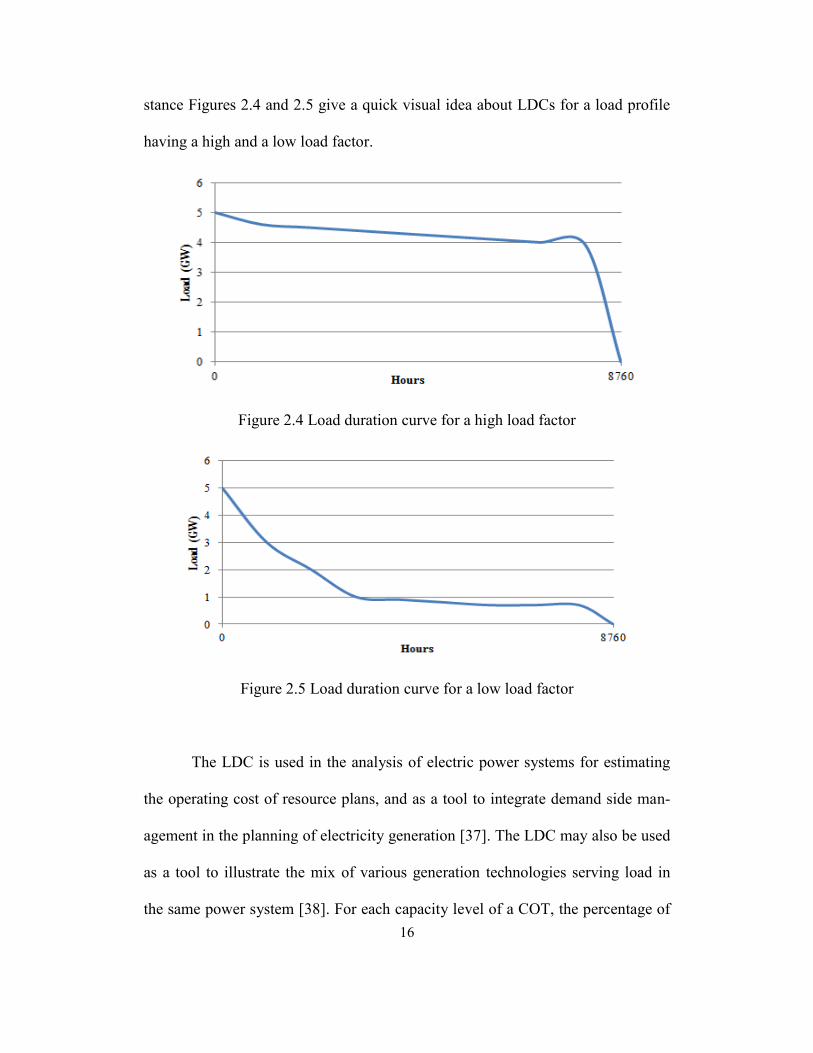
Load factor, which is calculated as the ratio of the average load to the peak

load in a power system during a period [36], indicates the nature of a load profile.

For example, a high load factor signifies a fairly constant load profile since the

average load is same as the peak load.

On the other hand, a LDC is a graphical representation and provides an

objective idea about the magnitude as well as the nature of load profile. For in-

16

stance Figures 2.4 and 2.5 give a quick visual idea about LDCs for a load profile

having a high and a low load factor.

Figure 2.4 Load duration curve for a high load factor

Figure 2.5 Load duration curve for a low load factor

The LDC is used in the analysis of electric power systems for estimating

the operating cost of resource plans, and as a tool to integrate demand side man-

agement in the planning of electricity generation [37]. The LDC may also be used

as a tool to illustrate the mix of various generation technologies serving load in

the same power system [38]. For each capacity level of a COT, the percentage of

17

time for each demand level is inferred from the LDC and subsequently used to

calculate the LOLP of the power system under study.

2.4 Loss of load probability

The LOLP is a probabilistic measure of load unavailability within a speci-

fied period of time. Based on the size of the system under evaluation and the ex-

tent of input data (generation availability model, outage probability and load data)

available, any of the following approaches can be employed to calculate LOLP:

Instead of building an equivalent generation distribution model first, the

load probability distribution may be convolved with the individual genera-

tion distribution one at a time and the resultant be convolved with the load

curve [20].

An equivalent generation capacity table can be constructed and the LOLP

can be deduced with the aid of the LDC.

The first method is suited for a system having a large number of generators. On

the other hand, the second method may involve extensive calculation for a system

having a large number of generators or multiple operating states.

As explained in the later sections, the LOLP calculation methodology pro-

posed in this thesis is accurately calculated using the second method since a fewer

number of generators is incorporated while constructing the test case and a differ-

ent approach has been undertaken to handle the existence of multiple operating

18

states of generating units. Hence to calculate the LOLP, the following simplistic

procedure is followed:

a) On the basis of the available generation data and the FOR of individual

generators connected to the power system under study, the capacity outage table

is constructed as depicted in Section 2.2.

b) The first column of the COT tabulates the combination of the generation

states possible. For each of the available generation states, the LDC is used to find

the amount of ‘time’ for which the load exceeds the available generation. This

adds a third column to the COT.

c) The probability of generation availability (column 2) is multiplied with the

corresponding values of time for which load exceeds generation (column 3). The

cumulative sum of all such products yields the LOLP. The unit of LOLP depends

on the unit of time used in the LDC.

2.5 Problems in developing reliability indices for wind generation

Wind is a variable form of energy and is continuously changing in an un-

predictable manner. Using the conventional LOLP calculation method for wind

generation systems would result in inaccurate results. This is primarily due to the

following approximations for wind systems which result in large deviations:

a) Inaccurate representation of wind generation availability data

Wind varies with the time of day (blows harder in night than in day) and is

influenced by seasonal variations. For example, in many parts of Texas, the aver-

19

age wind speed in March is around 14 m/s while it reduces to around 10 m/s in

September [39]. Hence the actual output of any wind farm is lower than its in-

stalled capacity and may never generate continuously up to its nameplate rating.

As illustrated in Section 2.4, for conventional generation systems the

LOLP is calculated by utilizing the available generation states from the COT

along with the LDC. Assuming the most ideal case where no partial loading of

generating units exists (except for wind generators), the generation states are in

turn derived from the values of installed generation capacity of individual ma-

chines. For wind generation the output is below its installed capacity most of the

time; therefore the LOLP calculation methodology requires a different approach

and is discussed in the subsequent sections.

b) Inaccurate FOR representation

Due to the variable non availability of the wind generator output, a binary

representation of forced outage rates for each wind generator would lead to erro-

neous results in LOLP calculation. Also neglecting the reduced output of wind

generators altogether would result in large errors too. In such a scenario, the cases

of reduced output of the wind generators must be visualized as cases of partial

outage and a model is needed to be developed accordingly. This thesis uses the

EFOR over a time interval to accurately denote the FOR.

20

2.6 LOLP calculation methodology for wind generation profile

LOLP calculation requires accurate data of the available generation and

the FOR of each generating unit. This section proposes a method to calculate

LOLP for wind integrated systems.

The approach followed is based on calculating the LOLP based on genera-

tion data available for a 24 hour period (other desired time spans may also be

suitably chosen). Within a day, the available generation changes enormously and

creates uncertainty regarding which precise value of generation should be chosen

to construct the COT. To tackle this problem, it is proposed to segregate the anal-

ysis period (24 hours used here) into multiple time intervals. Depending upon the

length of each time interval chosen, the available generation and the equivalent

forced outage rate is approximated as described in subsequent sections.

2.7 Segregation of wind generation profile into intervals

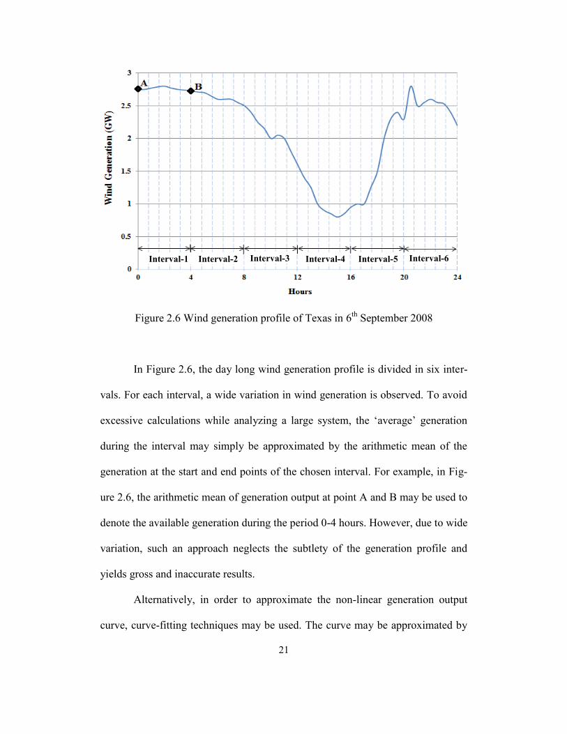
Figure 2.6 shows the wind generation profile of entire state of Texas for

6th

September 2008 [40]. It is noteworthy to observe the large variation in wind

generation data in daytime as compared to the night.

21

Figure 2.6 Wind generation profile of Texas in 6th

September 2008

In Figure 2.6, the day long wind generation profile is divided in six inter-

vals. For each interval, a wide variation in wind generation is observed. To avoid

excessive calculations while analyzing a large system, the ‘average’ generation

during the interval may simply be approximated by the arithmetic mean of the

generation at the start and end points of the chosen interval. For example, in Fig-

ure 2.6, the arithmetic mean of generation output at point A and B may be used to

denote the available generation during the period 0-4 hours. However, due to wide

variation, such an approach neglects the subtlety of the generation profile and

yields gross and inaccurate results.

Alternatively, in order to approximate the non-linear generation output

curve, curve-fitting techniques may be used. The curve may be approximated by

Interval-1 Interval-2 Interval-3 Interval-4 Interval-5 Interval-6

22

using a piece-wise cubic spline. A cubic spline is preferred since they are twice

differentiable polynomial curves and do not exhibit the oscillatory behavior ob-

served for higher order curves [41]. Further, being a lower order curve, splines are

easier to compute.

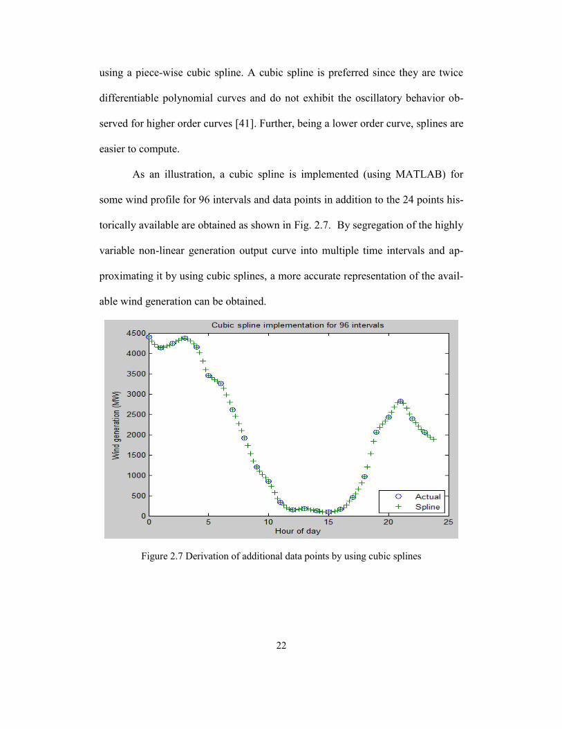
As an illustration, a cubic spline is implemented (using MATLAB) for

some wind profile for 96 intervals and data points in addition to the 24 points his-

torically available are obtained as shown in Fig. 2.7. By segregation of the highly

variable non-linear generation output curve into multiple time intervals and ap-

proximating it by using cubic splines, a more accurate representation of the avail-

able wind generation can be obtained.

Figure 2.7 Derivation of additional data points by using cubic splines

23

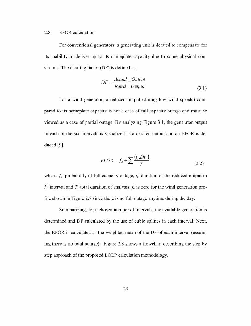
2.8 EFOR calculation

For conventional generators, a generating unit is derated to compensate for

its inability to deliver up to its nameplate capacity due to some physical con-

straints. The derating factor (DF) is defined as,

OutputRated

OutputActualDF

_

_

(3.1)

For a wind generator, a reduced output (during low wind speeds) com-

pared to its nameplate capacity is not a case of full capacity outage and must be

viewed as a case of partial outage. By analyzing Figure 3.1, the generator output

in each of the six intervals is visualized as a derated output and an EFOR is de-

duced [9],

T

DFtfEFOR i .

0 (3.2)

where, fo: probability of full capacity outage, ti: duration of the reduced output in

ith

interval and T: total duration of analysis. fo is zero for the wind generation pro-

file shown in Figure 2.7 since there is no full outage anytime during the day.

Summarizing, for a chosen number of intervals, the available generation is

determined and DF calculated by the use of cubic splines in each interval. Next,

the EFOR is calculated as the weighted mean of the DF of each interval (assum-

ing there is no total outage). Figure 2.8 shows a flowchart describing the step by

step approach of the proposed LOLP calculation methodology.

24

Start

Divide

generation

profile into

desired

intervals

Hourly

generation data

of each wind

generator

Desired

intervals

Use cubic splines to obtain

the available generation for

each interval

Calculate DF of each

interval. Calculate

EFOR of entire unit.

Construct

COT

Obtain time for

which load exceed

generation

Calculate

LOLP= ∑(p)(t)

Load

duration

curve

End

Figure 2.8 Flowchart depicting the proposed methodology of LOLP calculation

25

CHAPTER 3

TEST BED, SIMULATION AND RESULTS

3.1 Reliability calculation through proposed method

In this chapter, the reliability calculation methodology, which was dis-

cussed in the preceding section, is implemented on an existing power system test

case to illustrate the following:

Application and efficiency of the method to calculate the EFOR and sub-

sequently obtaining the LOLP for the system under study

The effect on LOLP due to increase in the installed capacity of wind ener-

gy generation

The variation of the EFOR and LOLP due to the change in the number of

intervals while implementing the algorithm

Dependency of LOLP on the type of wind generation profile

To successfully demonstrate the performance of the proposed method, a

test case having a fairly large size, a sufficiently high level of wind penetration

and a diverse variation of wind generation profile over the day is chosen to pro-

vide realistic results. Incorporating all such features, the Texas power system has

been used as a test case.

3.2 Choice of the Texas power system as test case

Texas is blessed with a plentiful of wind energy resource. With a high av-

erage wind speed ranging from 10 to 14 m/s in most parts of the state throughout

26

the year [42], one of the largest wind energy installations in the US is located in

Texas. The installed capacity of the Texas power system was around 105 GW in

2008 of which the installed wind generation capacity was nearly 7.5 GW [43] - a

wind penetration level of 6.8%. Further, according to the RPS goals, Texas has an

aggressive target of increasing wind energy installation in coming years [44]. This

factor makes Texas a better fit for conducting a realistic experiment to analyze the

effect of increased wind penetration on reliability of the expanded system.

For conducting LOLP calculations on the Texas power system, actual

hourly wind generation data [40] and hourly load profile [45] for the year 2008

have been procured from Electrical Reliability Council of Texas (ERCOT).

3.3 Description of test case

While constructing the test bed, an attempt has been made to simulate a

case most identical with the actual data of the Texas power system. Table 3.1 de-

picts the installed capacity of the chief energy sources serving Texas in 2008 [46]

and Table 3.2 lists the typical values of FORs [47] for those energy sources.

Table 3.1 Installed capacity of Texas power system in 2008

Energy source name Installed capacity (GW)

Nuclear 4.927

Coal 20.189

Natural gas 70.856

Wind 7.427

Total= 103.4

27

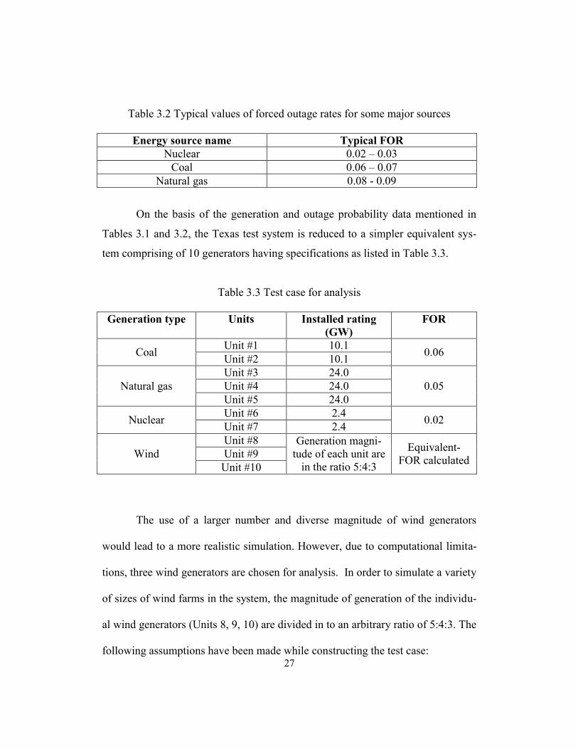
Table 3.2 Typical values of forced outage rates for some major sources

Energy source name Typical FOR

Nuclear 0.02 – 0.03

Coal 0.06 – 0.07

Natural gas 0.08 - 0.09

On the basis of the generation and outage probability data mentioned in

Tables 3.1 and 3.2, the Texas test system is reduced to a simpler equivalent sys-

tem comprising of 10 generators having specifications as listed in Table 3.3.

Table 3.3 Test case for analysis

Generation type Units Installed rating

(GW)

FOR

Coal Unit #1 10.1

0.06 Unit #2 10.1

Natural gas

Unit #3 24.0

0.05 Unit #4 24.0

Unit #5 24.0

Nuclear Unit #6 2.4

0.02 Unit #7 2.4

Wind

Unit #8 Generation magni-

tude of each unit are

in the ratio 5:4:3

Equivalent-

FOR calculated Unit #9

Unit #10

The use of a larger number and diverse magnitude of wind generators

would lead to a more realistic simulation. However, due to computational limita-

tions, three wind generators are chosen for analysis. In order to simulate a variety

of sizes of wind farms in the system, the magnitude of generation of the individu-

al wind generators (Units 8, 9, 10) are divided in to an arbitrary ratio of 5:4:3. The

following assumptions have been made while constructing the test case:

28

In order to simplify the test case for analysis, only the major energy

sources have been accounted for. Such an approximation has very little

effect on the accuracy of results since in the above test case around 103.4

GW of generation out of the actual installed 105 GW is already included.

For all units except for wind generators, derated or partially loaded opera-

tion has been neglected. Hence, while serving the power system, Units #1-

7 operate either in a state of being fully committed or having a full outage.

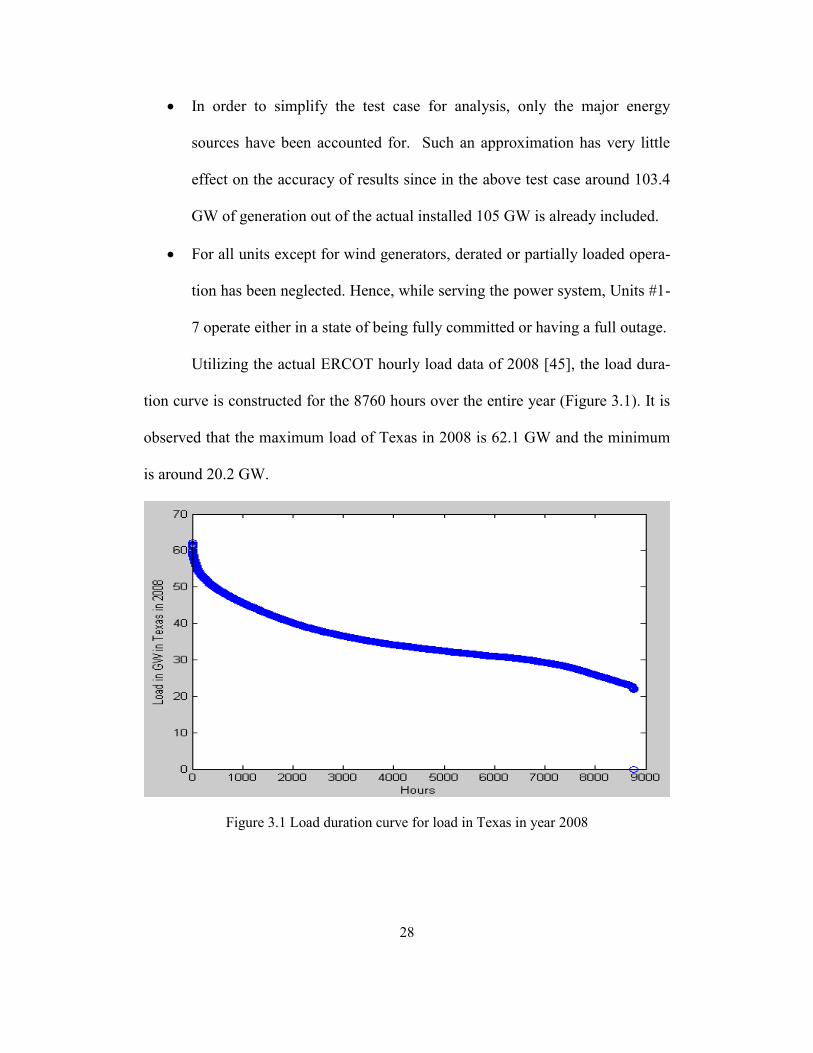
Utilizing the actual ERCOT hourly load data of 2008 [45], the load dura-

tion curve is constructed for the 8760 hours over the entire year (Figure 3.1). It is

observed that the maximum load of Texas in 2008 is 62.1 GW and the minimum

is around 20.2 GW.

Figure 3.1 Load duration curve for load in Texas in year 2008

29

3.4 Simulation showing LOLP and EFOR variation for the Texas test case

The highly variable pattern of wind profile necessitates that the proposed

methodology be simulated and the reliability index be calculated for the test case

for two types of wind generation profiles – one having a wide variation of wind

generation output over the entire day and another having a relatively ‘flat’ wind

generation profile. Such an approach provides an opportunity to evaluate the per-

formance of the method for varied patterns of wind generation outputs.

3.4.1 Case #1: 9th

June 2008

From the available hourly wind generation data [40], the wind generation

profile is constructed graphically as shown in Figure 3.2. The wind generation is

observed to be swinging from a maximum value of 4.37 GW to a minimum of

0.97 GW during the 24 hour period.

Figure 3.2 Hourly wind generation of Texas on 9th June 2008

30

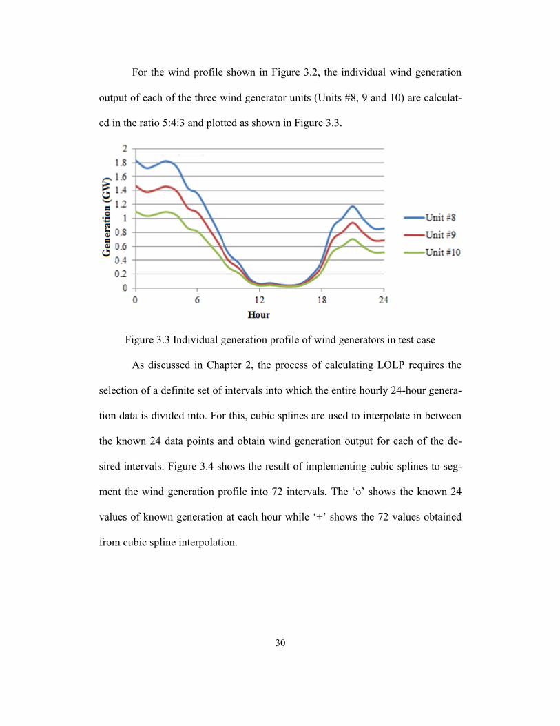
For the wind profile shown in Figure 3.2, the individual wind generation

output of each of the three wind generator units (Units #8, 9 and 10) are calculat-

ed in the ratio 5:4:3 and plotted as shown in Figure 3.3.

Figure 3.3 Individual generation profile of wind generators in test case

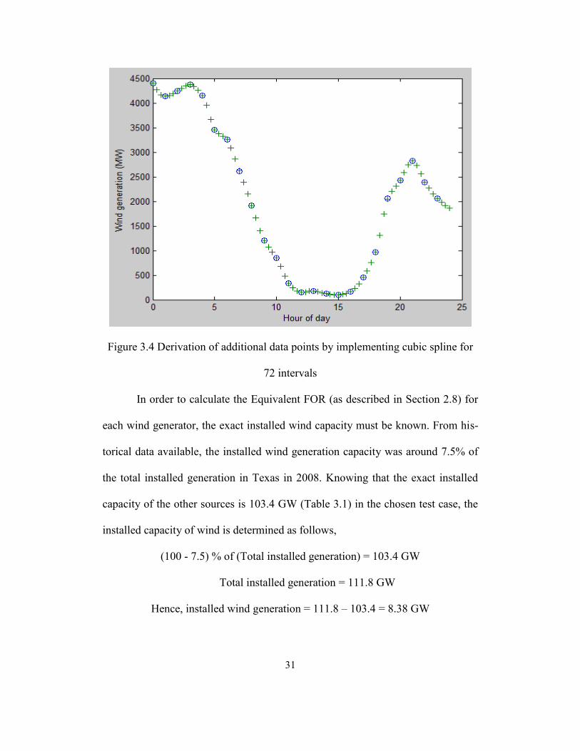
As discussed in Chapter 2, the process of calculating LOLP requires the

selection of a definite set of intervals into which the entire hourly 24-hour genera-

tion data is divided into. For this, cubic splines are used to interpolate in between

the known 24 data points and obtain wind generation output for each of the de-

sired intervals. Figure 3.4 shows the result of implementing cubic splines to seg-

ment the wind generation profile into 72 intervals. The ‘o’ shows the known 24

values of known generation at each hour while ‘+’ shows the 72 values obtained

from cubic spline interpolation.

31

Figure 3.4 Derivation of additional data points by implementing cubic spline for

72 intervals

In order to calculate the Equivalent FOR (as described in Section 2.8) for

each wind generator, the exact installed wind capacity must be known. From his-

torical data available, the installed wind generation capacity was around 7.5% of

the total installed generation in Texas in 2008. Knowing that the exact installed

capacity of the other sources is 103.4 GW (Table 3.1) in the chosen test case, the

installed capacity of wind is determined as follows,

(100 - 7.5) % of (Total installed generation) = 103.4 GW

Total installed generation = 111.8 GW

Hence, installed wind generation = 111.8 – 103.4 = 8.38 GW

32

Next, for each of the 72 intervals (for example), the DF and the EFOR is

calculated using (3.1) and (3.2),

capacityInstalled

generationActualDF

_

_

(3.1)

T

DFtfEFOR i .

0

(3.2)

where, ti is the duration of the derated hours. For 72 intervals, the value of ti is =

(24/72) hours. The forced outage rate f0 is zero since for the wind generation pro-

file under study, the wind generators are continuously operating and never have a

complete outage.

On calculating for the case of 72 intervals, the EFOR for the wind genera-

tor Unit #8 is obtained as 0.253708. It must be noted that this value is very high as

compared to the FOR of conventional generation units which typically ranges

around 0.02-0.07. Such a high outage probability for wind generator clearly indi-

cates that calculating LOLP (for a wind generation integrated system) through

conventional methods would result in extremely high error in reliability studies

and incorrectly yield an ‘optimistic’ picture of power system performance.

The data derived up to this point are sufficient to construct the COT for

the 10 generators under study and subsequently calculate the LOLP. The above

procedure is repeated for a varied number of intervals (4, 6, 12, 24, 32, 48, 72 and

96), and the following variation of LOLP and EFOR is observed as depicted in

Figure 3.5 and 3.6.

33

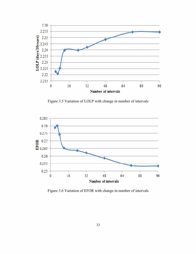
Figure 3.5 Variation of LOLP with change in number of intervals

Figure 3.6 Variation of EFOR with change in number of intervals

34

The results depicted in Figures 3.5 and 3.6 are for a fixed penetration level

of 7.5%. The following points must be noted:

The EFOR values are much higher than the typical values of FOR of con-

ventional generators.

The LOLP value for this test case is observed to be around 2.25 days/10yr

which is indeed quite high compared to typical values of LOLP for a pow-

er system in US. The reason may be attributed to a lesser number of gen-

erators used in the test case.

For a given penetration level, the LOLP increases and EFOR decreases as

number of intervals is increased. This may be seen as an indication that the

accuracy of calculation improves with an increase in the number of inter-

vals and leads to a higher LOLP (hence more unreliable) due to addition

of the variable wind energy.

After 72 intervals, the values of LOLP and EFOR are observed to stabilize

and seem to be the ‘optimal’ number of intervals for this case.

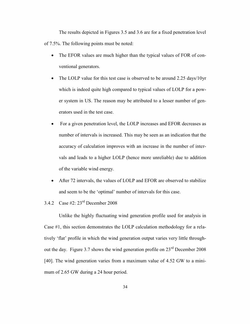
3.4.2 Case #2: 23rd

December 2008

Unlike the highly fluctuating wind generation profile used for analysis in

Case #1, this section demonstrates the LOLP calculation methodology for a rela-

tively ‘flat’ profile in which the wind generation output varies very little through-

out the day. Figure 3.7 shows the wind generation profile on 23rd

December 2008

[40]. The wind generation varies from a maximum value of 4.52 GW to a mini-

mum of 2.65 GW during a 24 hour period.

35

Figure 3.7 Hourly wind generation of Texas on 23rd

December 2008

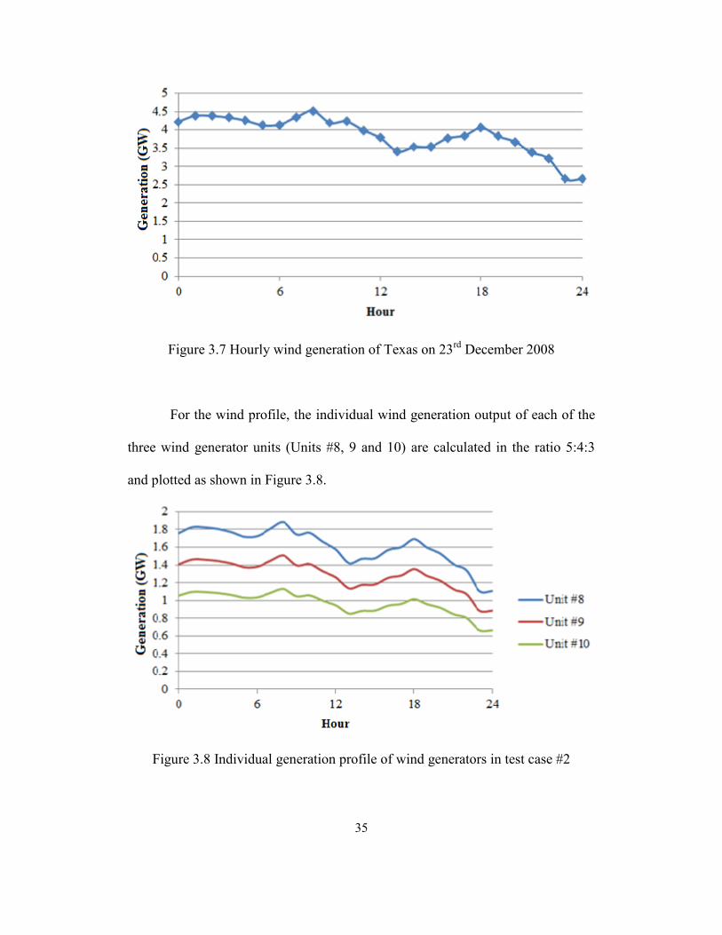
For the wind profile, the individual wind generation output of each of the

three wind generator units (Units #8, 9 and 10) are calculated in the ratio 5:4:3

and plotted as shown in Figure 3.8.

Figure 3.8 Individual generation profile of wind generators in test case #2

36

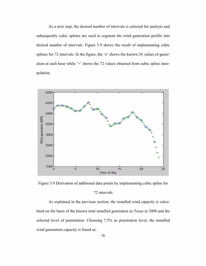
As a next step, the desired number of intervals is selected for analysis and

subsequently cubic splines are used to segment the wind generation profile into

desired number of intervals. Figure 3.9 shows the result of implementing cubic

splines for 72 intervals. In the figure, the ‘o’ shows the known 24 values of gener-

ation at each hour while ‘+’ shows the 72 values obtained from cubic spline inter-

polation.

Figure 3.9 Derivation of additional data points by implementing cubic spline for

72 intervals

As explained in the previous section, the installed wind capacity is calcu-

lated on the basis of the known total installed generation in Texas in 2008 and the

selected level of penetration. Choosing 7.5% as penetration level, the installed

wind generation capacity is found as:

37

(100 - 7.5) % of (Total installed generation) = 103.4 GW

Total installed generation = 111.8 GW

Hence, installed wind generation = 111.8 – 103.4 = 8.38 GW

Next, knowing the installed wind generation, the DF is calculated using

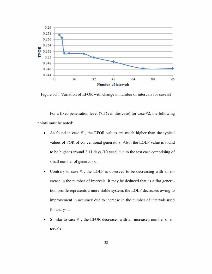
(3.1) for each of the 72 intervals (say). Subsequently the EFOR is evaluated using

(3.2). For the case of 72 intervals, the EFOR for wind generator Unit #8 is ob-

tained as 0.246. Similar to Case #1, the EFOR value is found to be much higher

than the FOR of conventional generation units which typically ranges around

0.02-0.07.

From the data derived up to this point, the COT is constructed for the 10

generator test system and the LOLP is subsequently calculated. Repeating the

above procedure for a varied number of intervals (4, 6, 12, 24, 32, 48, 72 and 96),

the following variation of LOLP and EFOR is observed as depicted in Figures

3.10 and 3.11 respectively.

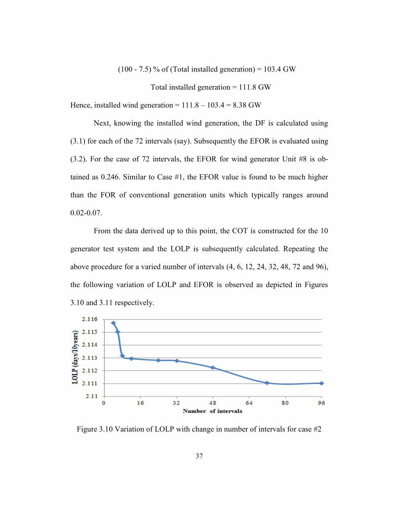
Figure 3.10 Variation of LOLP with change in number of intervals for case #2

38

Figure 3.11 Variation of EFOR with change in number of intervals for case #2

For a fixed penetration level (7.5% in this case) for case #2, the following

points must be noted:

As found in case #1, the EFOR values are much higher than the typical

values of FOR of conventional generators. Also, the LOLP value is found

to be higher (around 2.11 days /10 year) due to the test case comprising of

small number of generators.

Contrary to case #1, the LOLP is observed to be decreasing with an in-

crease in the number of intervals. It may be deduced that as a flat genera-

tion profile represents a more stable system, the LOLP decreases owing to

improvement in accuracy due to increase in the number of intervals used

for analysis.

Similar to case #1, the EFOR decreases with an increased number of in-

tervals.

39

Like case #1, the values of LOLP and EFOR are observed to stabilize after

72 intervals and thus seem to be the ‘optimal’ number of intervals for this

test case.

3.5 Results depicting the effect of increased wind penetration

The penetration of wind is expected to increases aggressively in Texas in

the coming years. In the event of such an expansion, it is necessary to evaluate the

generation adequacy of the existing power system infrastructure. This section pre-

sents the results of the pattern of change in LOLP with an increase in wind ca-

pacity penetration from 5% to 10% for different wind generation profiles.

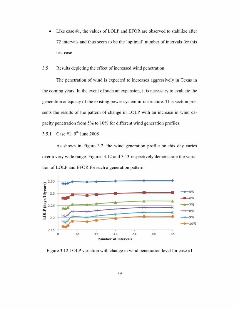
3.5.1 Case #1: 9th

June 2008

As shown in Figure 3.2, the wind generation profile on this day varies

over a very wide range. Figures 3.12 and 3.13 respectively demonstrate the varia-

tion of LOLP and EFOR for such a generation pattern.

Figure 3.12 LOLP variation with change in wind penetration level for case #1

40

Figure 3.13 EFOR variation with change in wind penetration level for case #1

3.5.2 Case #2: 23rd

December 2008

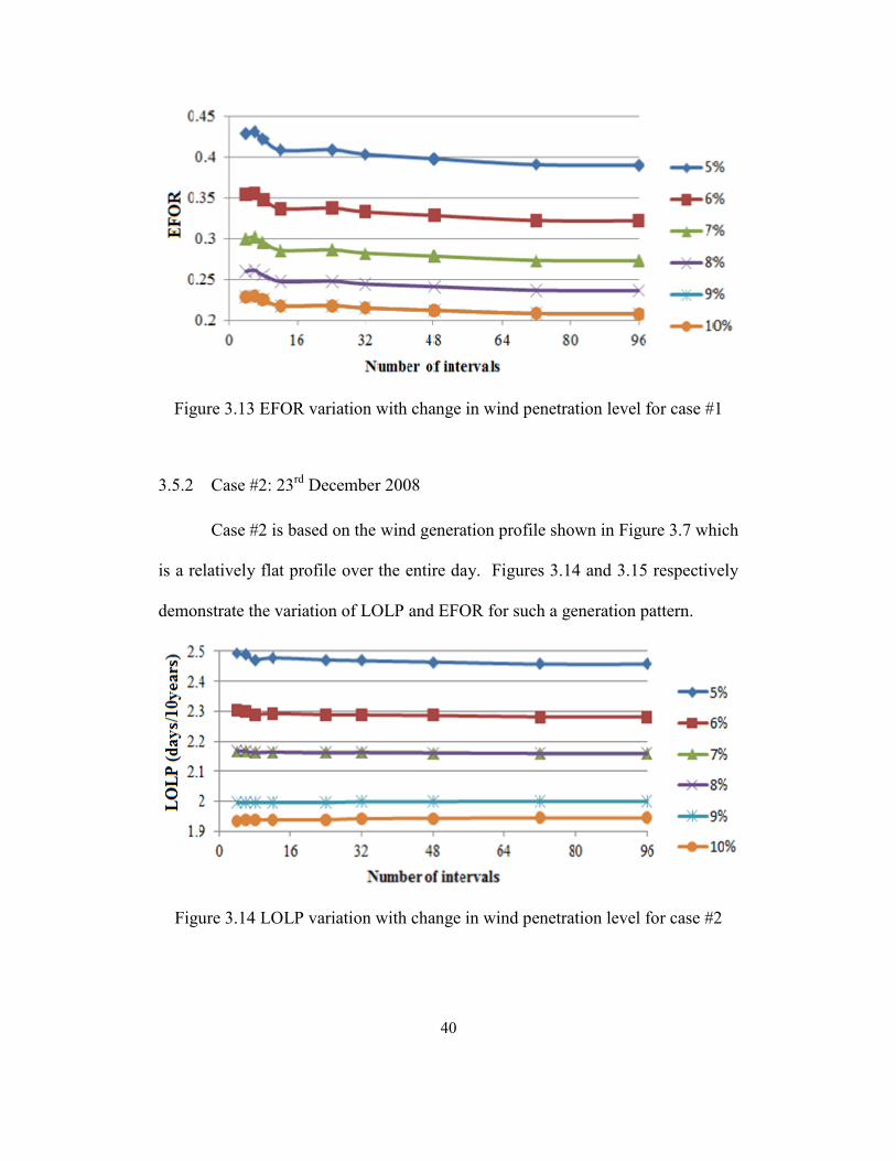
Case #2 is based on the wind generation profile shown in Figure 3.7 which

is a relatively flat profile over the entire day. Figures 3.14 and 3.15 respectively

demonstrate the variation of LOLP and EFOR for such a generation pattern.

Figure 3.14 LOLP variation with change in wind penetration level for case #2

41

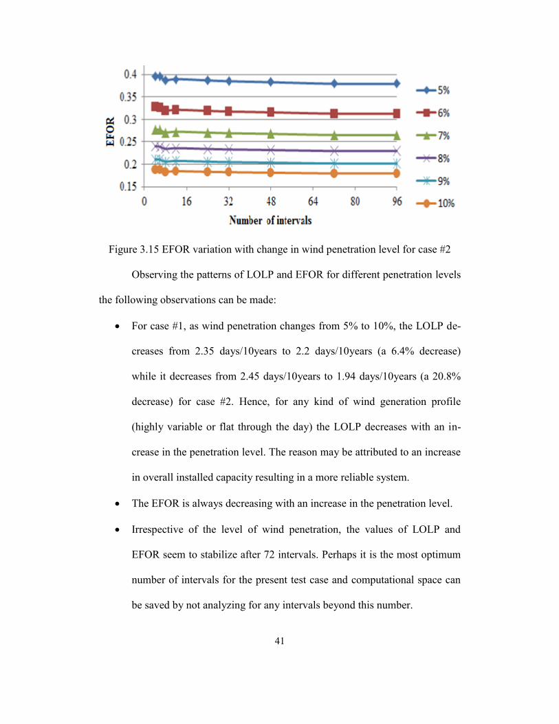
Figure 3.15 EFOR variation with change in wind penetration level for case #2

Observing the patterns of LOLP and EFOR for different penetration levels

the following observations can be made:

For case #1, as wind penetration changes from 5% to 10%, the LOLP de-

creases from 2.35 days/10years to 2.2 days/10years (a 6.4% decrease)

while it decreases from 2.45 days/10years to 1.94 days/10years (a 20.8%

decrease) for case #2. Hence, for any kind of wind generation profile

(highly variable or flat through the day) the LOLP decreases with an in-

crease in the penetration level. The reason may be attributed to an increase

in overall installed capacity resulting in a more reliable system.

The EFOR is always decreasing with an increase in the penetration level.

Irrespective of the level of wind penetration, the values of LOLP and

EFOR seem to stabilize after 72 intervals. Perhaps it is the most optimum

number of intervals for the present test case and computational space can

be saved by not analyzing for any intervals beyond this number.

42

CHAPTER 4

THEORY OF WIND GENERATION TECHNOLOGIES AND THE DFIG

POWER CONVERTER TOPOLOGY

4.1 Overview: wind turbine configurations

A wind generator may be broadly classified as a fixed speed or a variable

speed type. A fixed speed turbine is simple in construction and does not have a

power electronics converter for its control [29]. This design makes a cheaper con-

figuration than the variable speed systems. The fixed speed may also have some

advantages in lower losses. However, fixed speed machines extract the maximum

power only at a particular wind speed [23]. Hence, for a site where wind speeds

are highly variable, such a configuration does not deliver the optimal perfor-

mance. On the other hand, variable speed turbines use power electronics convert-

ers to control the electrical energy injected into the grid. Unlike the fixed speed

topologies, these systems can specifically control the voltage, frequency, active

power and reactive power output and easily enable smooth integration of even

large sized wind farms into the grid. Such turbine systems are costlier and inject

high harmonics into the power system. Broadly, wind turbine configurations [48],

[49] can be categorized as:

a) Type 1 turbine configuration

This topology typically consists of an asynchronous squirrel cage induc-

tion generator (SCIG) connected to a fixed speed wind turbine. With an active

stall control, these turbines have the ability to stop and start faster than the other

configurations. The major drawback of Type 1 turbines is that they operate at a

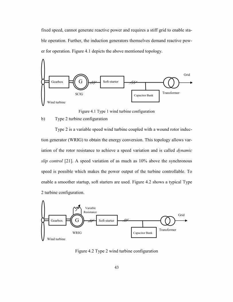
43

fixed speed, cannot generate reactive power and requires a stiff grid to enable sta-

ble operation. Further, the induction generators themselves demand reactive pow-

er for operation. Figure 4.1 depicts the above mentioned topology.

Figure 4.1 Type 1 wind turbine configuration

b) Type 2 turbine configuration

Type 2 is a variable speed wind turbine coupled with a wound rotor induc-

tion generator (WRIG) to obtain the energy conversion. This topology allows var-

iation of the rotor resistance to achieve a speed variation and is called dynamic

slip control [21]. A speed variation of as much as 10% above the synchronous

speed is possible which makes the power output of the turbine controllable. To

enable a smoother startup, soft starters are used. Figure 4.2 shows a typical Type

2 turbine configuration.

Figure 4.2 Type 2 wind turbine configuration

G

Variable

Resistance Grid

Wind turbine

WRIG Transformer

Gearbox Soft-starter

Capacitor Bank

Gearbox Soft-starter

Capacitor Bank

G

SCIG

Grid

Transformer

Wind turbine

44

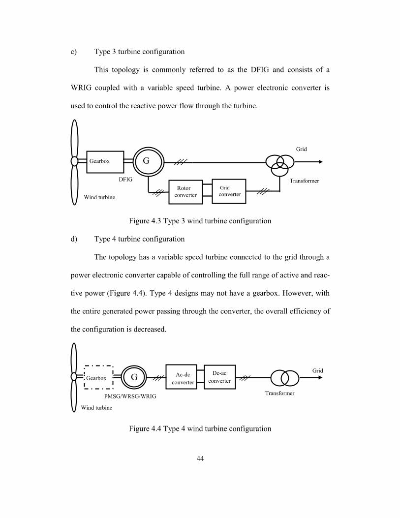
c) Type 3 turbine configuration

This topology is commonly referred to as the DFIG and consists of a

WRIG coupled with a variable speed turbine. A power electronic converter is

used to control the reactive power flow through the turbine.

Figure 4.3 Type 3 wind turbine configuration

d) Type 4 turbine configuration

The topology has a variable speed turbine connected to the grid through a

power electronic converter capable of controlling the full range of active and reac-

tive power (Figure 4.4). Type 4 designs may not have a gearbox. However, with

the entire generated power passing through the converter, the overall efficiency of

the configuration is decreased.

Figure 4.4 Type 4 wind turbine configuration

G Grid

PMSG/WRSG/WRIG

Wind turbine

Ac-dc

converter

Transformer

Gearbox

DFIG

Grid

G

Wind turbine

Rotor

converter

Transformer

Gearbox

Grid converter

Dc-ac

converter

45

4.2 The doubly fed induction generators

The DFIG based configuration (Type 3) enables an active tracking of the

wind speed to operate the rotor near its optimum tip speed ratio (TSR) and there-

by extract the maximum power. Depending on the site location and turbine aero-

dynamics, such a configuration can, on an average, collect around 10% more an-

nual energy [23]. Hence, of all the wind turbine configurations discussed in Sec-

tion 4.1, the Type 3 turbines (Figure 4.3) are the most economical and popular

form of topology in use [48] and are discussed in detail in this section.

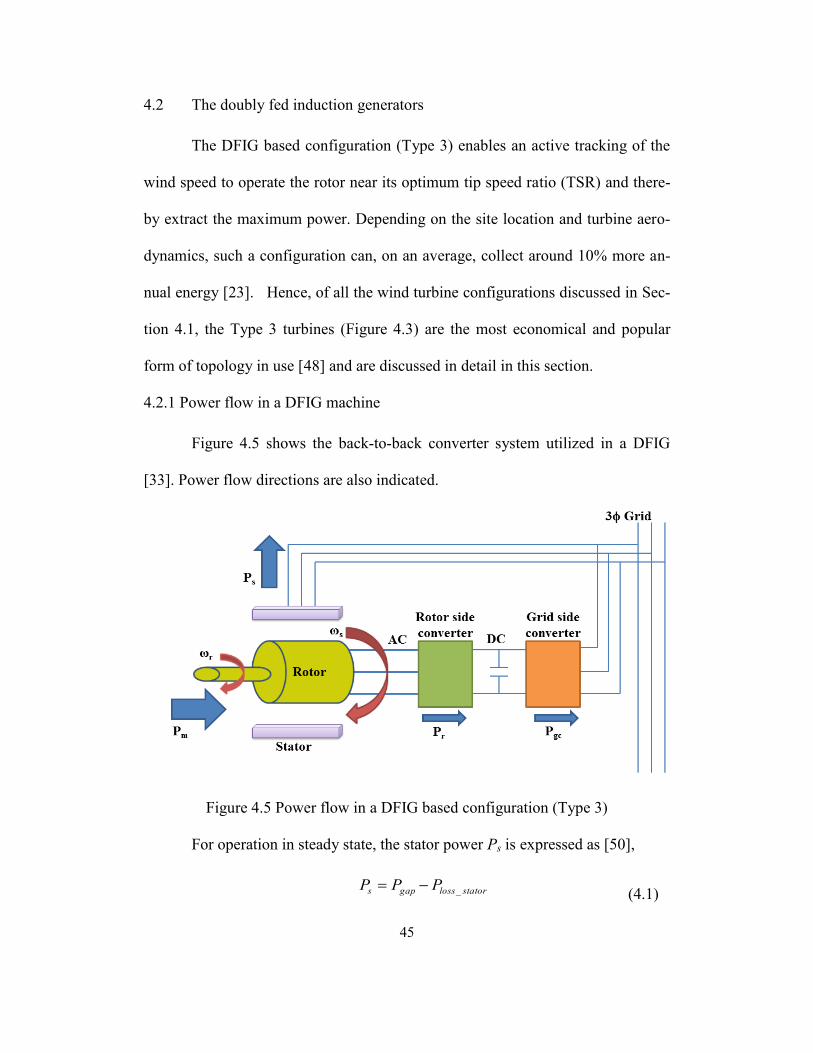
4.2.1 Power flow in a DFIG machine

Figure 4.5 shows the back-to-back converter system utilized in a DFIG

[33]. Power flow directions are also indicated.

Figure 4.5 Power flow in a DFIG based configuration (Type 3)

For operation in steady state, the stator power Ps is expressed as [50],

statorlossgaps PPP _ (4.1)

46

where, Pgap is the power transferred through the air gap and Ploss_stator is the copper

losses in the rotor circuit. The air gap power is defined in terms of the mechanical

power input from the wind turbine (Pm) and the power through the rotor (Pr) as,

rmgap PPP (4.2)

From (4.1) and (4.2) for negligible rotor losses the stator power is defined as,

rms PPP (4.3)

Defining the quantities in terms of the generator torque T, Ps and Pm are expressed

as,

ss TP (4.4)

rm TP (4.5)

where, ωs is the stator electrical frequency and ωr is the rotor electrical frequency.

Subtracting (4.4) and (4.5) and rearranging,

srsr sTTP )( (4.6)

where, s is the slip and is defined as,

s

rss

)(

(4.7)

From (4.3) and (4.6), (4.8) is obtained,

sr sPP

(4.8)

Combining (4.3) and (4.8), Pm can be expressed as,

srsm PsPPP )1(

(4.9)

47

As illustrated by (4.9), in a DFIG the electrical power output can be varied

by the control of the slip. Using (4.7), theoretically a rotor speed up to twice the

synchronous speed can be obtained by varying the slip from -1 to +1 (i.e., 7,200

rpm for 60 Hz electrical for one pole-pair). Such operation enables the rotor to

absorb as well as deliver power. On the basis of rotational speed of generator rela-

tive to the synchronous speed, the DFIG operation can be generalized as [51]:

At synchronous speed, the rotor current is dc as in a synchronous machine.

If losses are neglected, all of the mechanical power inputted by the turbine

to the rotor gets transferred to the grid via the stator. No power is ex-

changed directly between the rotor and the grid through the back-to-back

converters.

If the machine operates below the synchronous speed, it is known as the

subsynchronous operation. The stator generates power to feed the grid but

part of it is fed back to the rotor through the converters.

In the supersynchronous mode of operation (operating above synchronous

speed), both the rotor and the stator feed power to the grid.

Due to mechanical and economic reasons, there are restrictions on the

maximum slip achievable and the practical speed range of a DFIG varies typically

between -40% to 30% of the synchronous speed [48]. On the basis of (4.1)-(4.9),

Figures 4.6 and 4.7 depict the power flow in a DFIG for the subsynchronous and

supersynchronous operations.

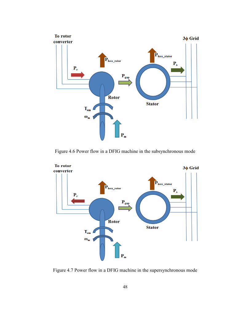
48

Figure 4.6 Power flow in a DFIG machine in the subsynchronous mode

Figure 4.7 Power flow in a DFIG machine in the supersynchronous mode

49

It must be noted that as derived in (4.9), Pr is dependent on the slip. Thus,

for subsynchronous speeds when the slip is positive, Pr is taken out of the rotor-

side converter and fed to the rotor. For supersynchronous speeds, Pr is transmitted

from the rotor to the dc bus.

4.2.2 The rotor side converter

The rotor side converter utilizes pre-defined power speed characteristics

(tracking characteristics) to derive the maximum power at any wind speed within

the operation range. For a wind turbine, the power output is related to the wind

speed as [52],

),(

2

1 3 Pmech CAvP (4.10)

where, Pmech is the turbine output power, is the density of air, A area covered

by the span of the turbine blades, v is the speed of the wind, CP is the power coef-

ficient, is the tip speed ratio and is the pitch angle of the blades.

It must be noted that while Pmech is the turbine power output, Pm is the net

power inputted into the generator rotor. For a lossless mechanical power transmis-

sion between the turbine and the generator rotor, Pmech is equal to Pm.

The power coefficient is expressed as [52],

i

c

i

P eccc

cC

5

432

1),(

(4.11)

where, the constants c1 =0.22, c2 =116, c3 =0.4, c4 =5 and c5 =12.5 and i is de-

fined as,

50

1

035.0

08.0

113

i (4.12)

The parameters for a General Electric (GE) 1.5MW wind turbine are available

from [53]. The values are listed in Table 4.1.

Table 4.1 Parameters for a 1.5 MW General Electric wind turbine

Parameter Value

A5.0 0.00159 kg/m

56.6 ωt /ν (m/s)-1

where, ωt is the angular turbine speed in per unit

On basis of above details, the turbine tracking characteristics the wind tur-

bine is constructed and is shown in Figure 4.8. Its operation is illustrated by defin-

ing four points A, B, C and D. The actual speed of rotor (ωr) is measured and the

corresponding optimal mechanical power from the tracking characteristics is used

as the reference power. When the power level is above 75% of the rated turbine

power, the speed reference is kept at 1.2 p.u. (region C to D). For operation in be-

tween 15% to 75%, the speed reference (region B to C) is [53],

51.042.167.0 _

2

_ pumpumref PP (4.13)

where, Pm_pu is the p.u. mechanical power inputted from the turbine into the rotor

and ωref is the generator speed reference in per unit.

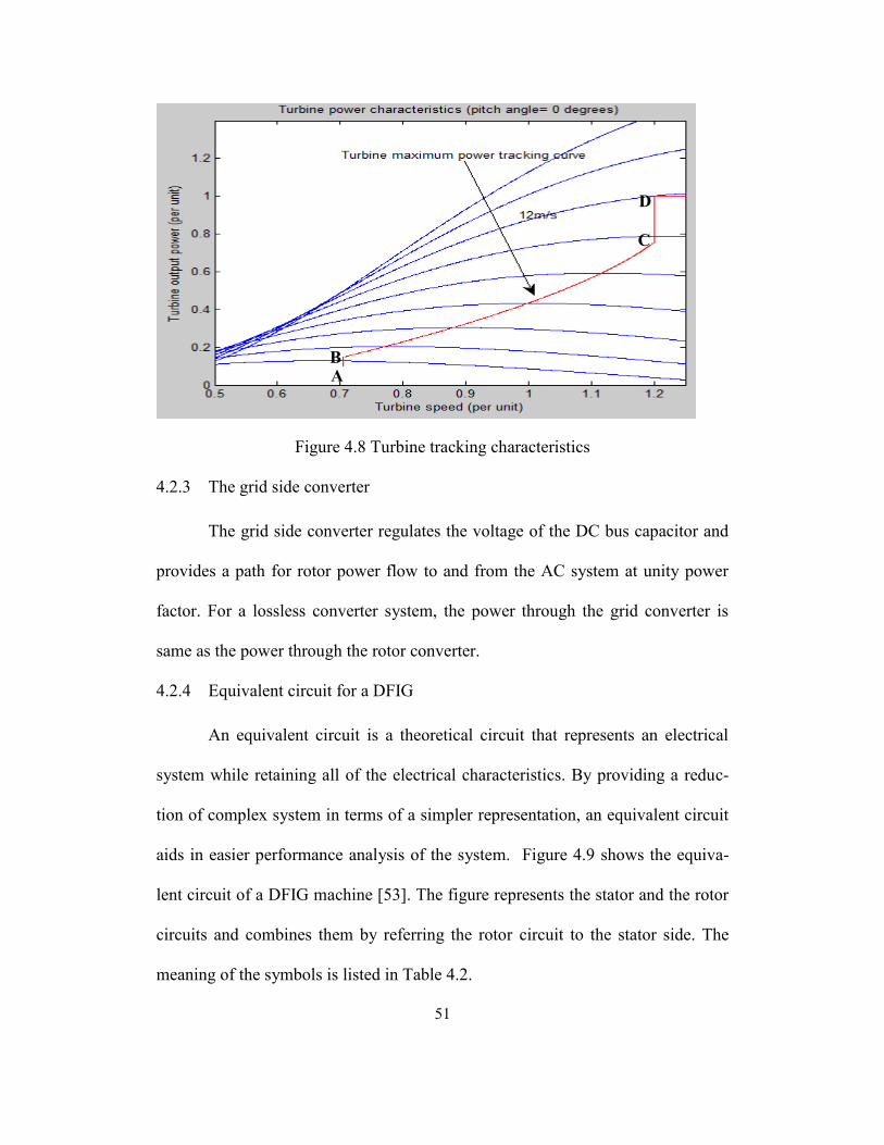
51

Figure 4.8 Turbine tracking characteristics

4.2.3 The grid side converter

The grid side converter regulates the voltage of the DC bus capacitor and

provides a path for rotor power flow to and from the AC system at unity power

factor. For a lossless converter system, the power through the grid converter is

same as the power through the rotor converter.

4.2.4 Equivalent circuit for a DFIG

An equivalent circuit is a theoretical circuit that represents an electrical

system while retaining all of the electrical characteristics. By providing a reduc-

tion of complex system in terms of a simpler representation, an equivalent circuit

aids in easier performance analysis of the system. Figure 4.9 shows the equiva-

lent circuit of a DFIG machine [53]. The figure represents the stator and the rotor

circuits and combines them by referring the rotor circuit to the stator side. The

meaning of the symbols is listed in Table 4.2.

A B

C

D

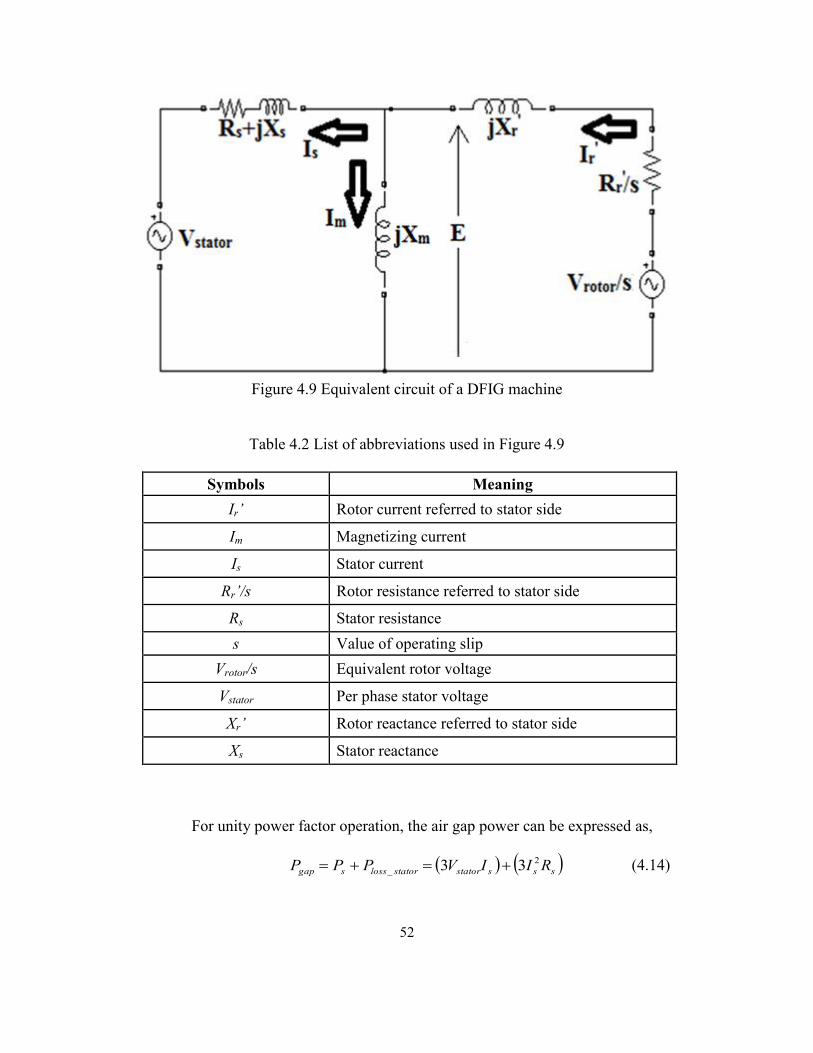
52

Figure 4.9 Equivalent circuit of a DFIG machine

Table 4.2 List of abbreviations used in Figure 4.9

Symbols Meaning

Ir’ Rotor current referred to stator side

Im Magnetizing current

Is Stator current

Rr’/s Rotor resistance referred to stator side

Rs Stator resistance

s Value of operating slip

Vrotor/s Equivalent rotor voltage

Vstator Per phase stator voltage

Xr’ Rotor reactance referred to stator side

Xs Stator reactance

For unity power factor operation, the air gap power can be expressed as,

sssstatorstatorlosssgap RIIVPPP 2

_ 33 (4.14)

53

The value of Is can be determined by solving the quadratic equation (4.14). The

voltage across the rotor circuit can be calculated as in (4.15),

sssstator IjXRVE )( (4.15)

The magnetizing current Im is calculated as,

m

mjX

EI (4.16)

As seen in Figure 4.9, for the chosen direction of power flow, the rotor current is

the addition of the magnetizing and the stator current,

msr III ' (4.17)

The slip dependent rotor voltage of the DFIG machine is calculated as,

''

'

)(/ rrr

rotor IjXs

REsV (4.18)

4.2.5 Phasor diagram of a DFIG machine

The phasor diagram for a DFIG machine can be constructed by utilizing

the derived equations in Section 4.2.4. For a DFIG delivering power to grid at

unity power factor, the stator current, Is, is aligned in the direction of the stator

voltage Vstator (which is the grid voltage). Using (4.15), the voltage drop across

stator impedance is added to Vstator to obtain the phasor corresponding to internal

electro motive force (EMF). The magnetizing current (Im) is calculated by using

(4.16) and its phasor is drawn 900

lagging to the magnetizing EMF (E). The rotor

current is found using (4.17). Lastly, as defined by (4.18), by incorporating the

voltage drops across the rotor impedances, the phasor corresponding to rotor volt-

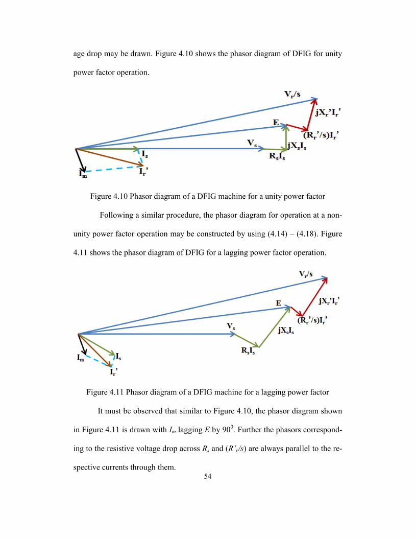
54

age drop may be drawn. Figure 4.10 shows the phasor diagram of DFIG for unity

power factor operation.

Figure 4.10 Phasor diagram of a DFIG machine for a unity power factor

Following a similar procedure, the phasor diagram for operation at a non-

unity power factor operation may be constructed by using (4.14) – (4.18). Figure

4.11 shows the phasor diagram of DFIG for a lagging power factor operation.

Figure 4.11 Phasor diagram of a DFIG machine for a lagging power factor

It must be observed that similar to Figure 4.10, the phasor diagram shown

in Figure 4.11 is drawn with Im lagging E by 900. Further the phasors correspond-

ing to the resistive voltage drop across Rs and (R’r/s) are always parallel to the re-

spective currents through them.

55

CHAPTER 5

CONSTRUCTION OF A GUI FOR THE DFIG GENERATION SYSTEM

5.1 Choice of MATLAB for GUI construction

This chapter explains the construction of a GUI to demonstrate the work-

ing of the DFIG machine, display its power flow and depict its maximum power

point tracking mechanism.

For developing a GUI, numerous programming languages are available.

Microsoft Visual Basic is the most preferred choice by advanced programmers.

Being a Microsoft product, Visual Basic is easily compatible with the Windows

operating system. Similarly JAVA based GUI are inherently implementable on

any operating system. However, both of these languages require an advanced skill

level to understand, develop or edit programs.

Focusing on choosing a simpler language to demonstrate engineering sys-

tems, this thesis uses the dedicated GUI toolbox of MATLAB for illustrating the

DFIG system. Due to the nature of the technical content desired to be simulated in

this thesis and the kind of end users expected to benefit from it, MATLAB offers

the following advantages:

MATLAB is easily available in universities and electrical engineering stu-

dents learn it as part of their course work. Hence, the drag-and-drop fea-

ture of the MATLAB GUI construction tool eliminates the need to learn

any new GUI language to understand or edit the program.

56

By using its powerful mathematical and engineering toolbox, MATLAB

offers scope for extending this GUI to simulate more complicated aspects

of the DFIG in the future.

MATLAB has the functionality of converting its GUI into standalone exe-

cutable files. This eliminates the necessity to install MATLAB on user

computer and makes the GUI accessible to users belonging to non-

engineering background also.

5.2 Features of the GUI for simulation of a DFIG system

The GUI is intended to aid the end user to visualize the electrical working

of a DFIG machine and understand its change in operational behavior for a varia-

ble range of wind speed inputs. Thus, the GUI has been constructed with four in-

terconnected program interfaces which dynamically modify their display for the

entered wind speeds. The GUI is constructed by choosing a wind turbine similar

to the GE wind turbine model 1.5sle. The specifications of the turbine are listed in

Table 5.1 [54].

Table 5.1 Specification of wind turbine used as test case for GUI design

Specifications Detail

Rated capacity 1.5 MW

Rated wind speed 12 m/s

57

5.2.1 The power flow interface

The interface shows the change in power transfer within the wind turbine

for a change in wind speed. The interface allows the user to vary the wind speed

from 6 to 14 m/s with the aid of a slider interface. Accordingly, the program cal-

culates the optimum slip to extract maximum power from the turbine by using the

theory explained in Section 4.2. The interface displays the following parameters

on the screen:

The optimum slip

The corresponding turbine speed in rad/s

The mechanical power inputted into generator rotor (Pm) for a given wind

speed (calculated using (4.10))

The air gap power (Pgap) as per the maximum power point tracking

The magnitude and direction of power transferred between the rotor and

the rotor converter (Pr)

Figures 5.1 and 5.2 show the snapshot of the constructed GUI and depict

the change in the direction of the Pr as the wind speed changes from 7 m/s to 10

m/s. The directions of the power flow are programmed to change as per the wind

speed variation. It must be noted that in Figure 5.1, the DFIG is operating in sub-

subsynchronous operation and power is directed from rotor converter to the rotor.

However, in Figure 5.2 when the machine is operating in a supersynchronous op-

eration, the rotor supplies power to the rotor converter. Consequently, in both the

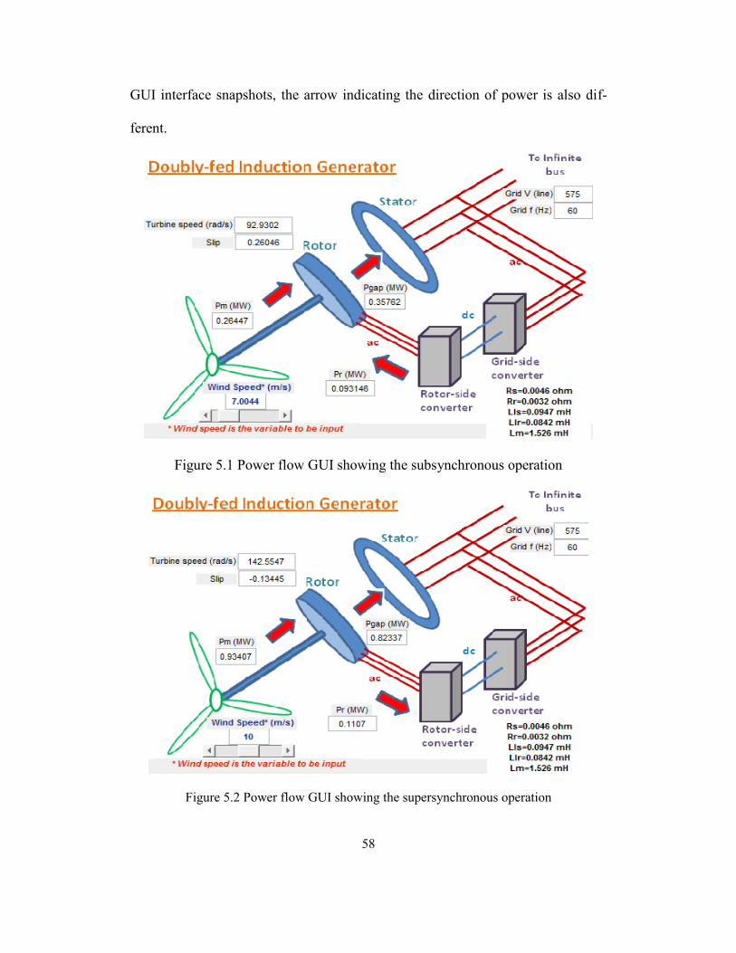
58

GUI interface snapshots, the arrow indicating the direction of power is also dif-

ferent.

Figure 5.1 Power flow GUI showing the subsynchronous operation

Figure 5.2 Power flow GUI showing the supersynchronous operation

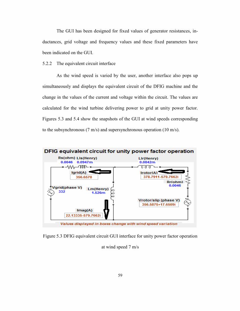
59

The GUI has been designed for fixed values of generator resistances, in-

ductances, grid voltage and frequency values and these fixed parameters have

been indicated on the GUI.

5.2.2 The equivalent circuit interface

As the wind speed is varied by the user, another interface also pops up

simultaneously and displays the equivalent circuit of the DFIG machine and the

change in the values of the current and voltage within the circuit. The values are

calculated for the wind turbine delivering power to grid at unity power factor.

Figures 5.3 and 5.4 show the snapshots of the GUI at wind speeds corresponding

to the subsynchronous (7 m/s) and supersynchronous operation (10 m/s).

Figure 5.3 DFIG equivalent circuit GUI interface for unity power factor operation

at wind speed 7 m/s

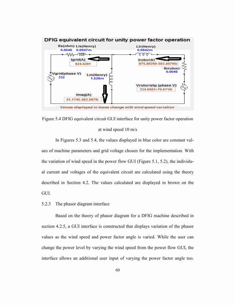
60

Figure 5.4 DFIG equivalent circuit GUI interface for unity power factor operation

at wind speed 10 m/s

In Figures 5.3 and 5.4, the values displayed in blue color are constant val-

ues of machine parameters and grid voltage chosen for the implementation. With

the variation of wind speed in the power flow GUI (Figure 5.1, 5.2), the individu-

al current and voltages of the equivalent circuit are calculated using the theory

described in Section 4.2. The values calculated are displayed in brown on the

GUI.

5.2.3 The phasor diagram interface

Based on the theory of phasor diagram for a DFIG machine described in

section 4.2.5, a GUI interface is constructed that displays variation of the phasor

values as the wind speed and power factor angle is varied. While the user can

change the power level by varying the wind speed from the power flow GUI, the

interface allows an additional user input of varying the power factor angle too.

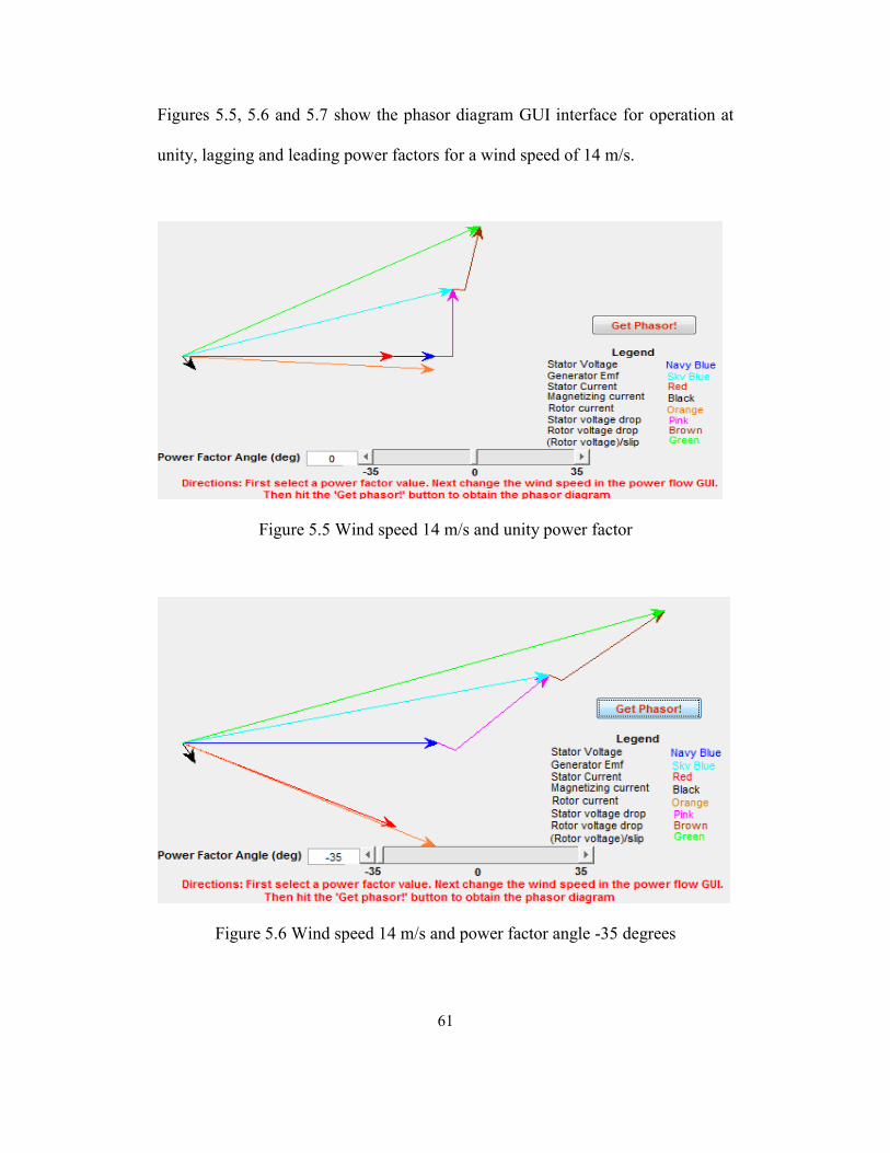
61

Figures 5.5, 5.6 and 5.7 show the phasor diagram GUI interface for operation at

unity, lagging and leading power factors for a wind speed of 14 m/s.

Figure 5.5 Wind speed 14 m/s and unity power factor

Figure 5.6 Wind speed 14 m/s and power factor angle -35 degrees

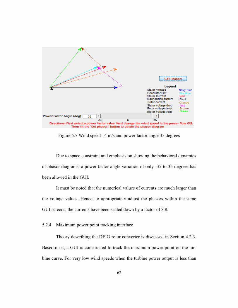
62

Figure 5.7 Wind speed 14 m/s and power factor angle 35 degrees

Due to space constraint and emphasis on showing the behavioral dynamics

of phasor diagrams, a power factor angle variation of only -35 to 35 degrees has

been allowed in the GUI.

It must be noted that the numerical values of currents are much larger than

the voltage values. Hence, to appropriately adjust the phasors within the same

GUI screens, the currents have been scaled down by a factor of 8.8.

5.2.4 Maximum power point tracking interface

Theory describing the DFIG rotor converter is discussed in Section 4.2.3.

Based on it, a GUI is constructed to track the maximum power point on the tur-

bine curve. For very low wind speeds when the turbine power output is less than

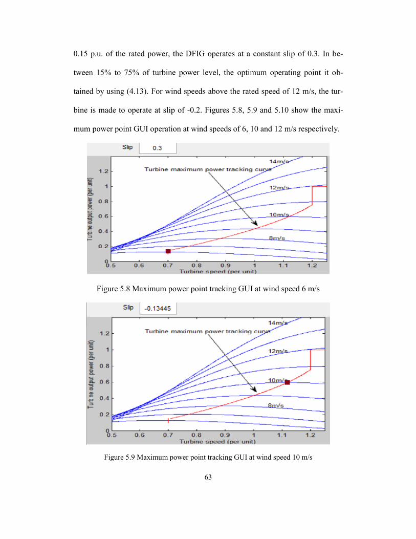
63

0.15 p.u. of the rated power, the DFIG operates at a constant slip of 0.3. In be-

tween 15% to 75% of turbine power level, the optimum operating point it ob-

tained by using (4.13). For wind speeds above the rated speed of 12 m/s, the tur-

bine is made to operate at slip of -0.2. Figures 5.8, 5.9 and 5.10 show the maxi-

mum power point GUI operation at wind speeds of 6, 10 and 12 m/s respectively.

Figure 5.8 Maximum power point tracking GUI at wind speed 6 m/s

Figure 5.9 Maximum power point tracking GUI at wind speed 10 m/s

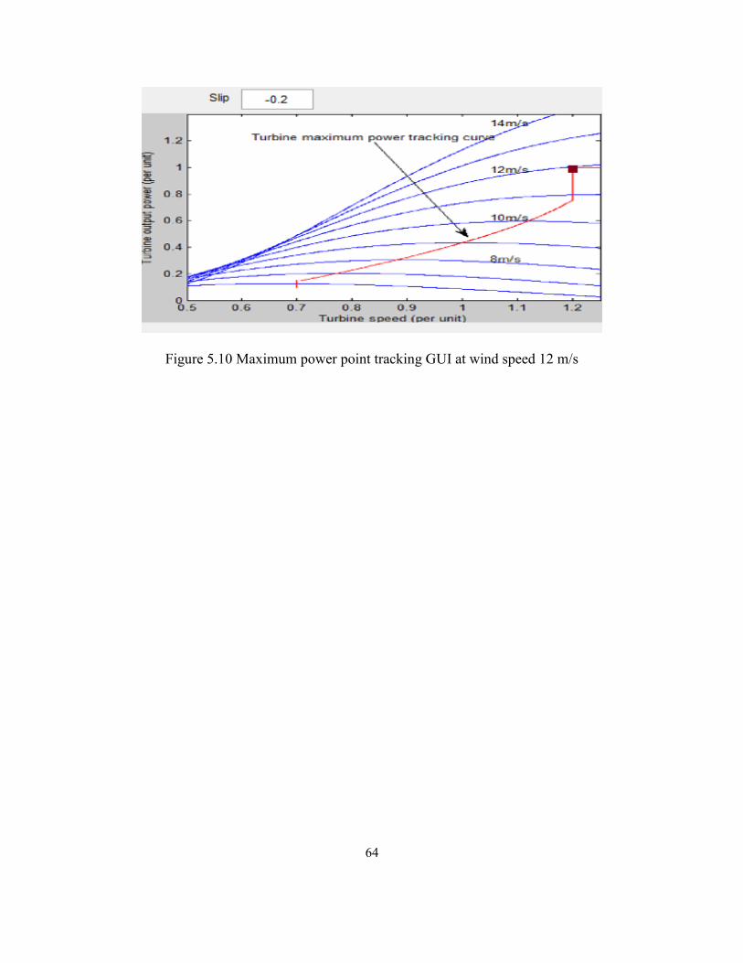
64

Figure 5.10 Maximum power point tracking GUI at wind speed 12 m/s

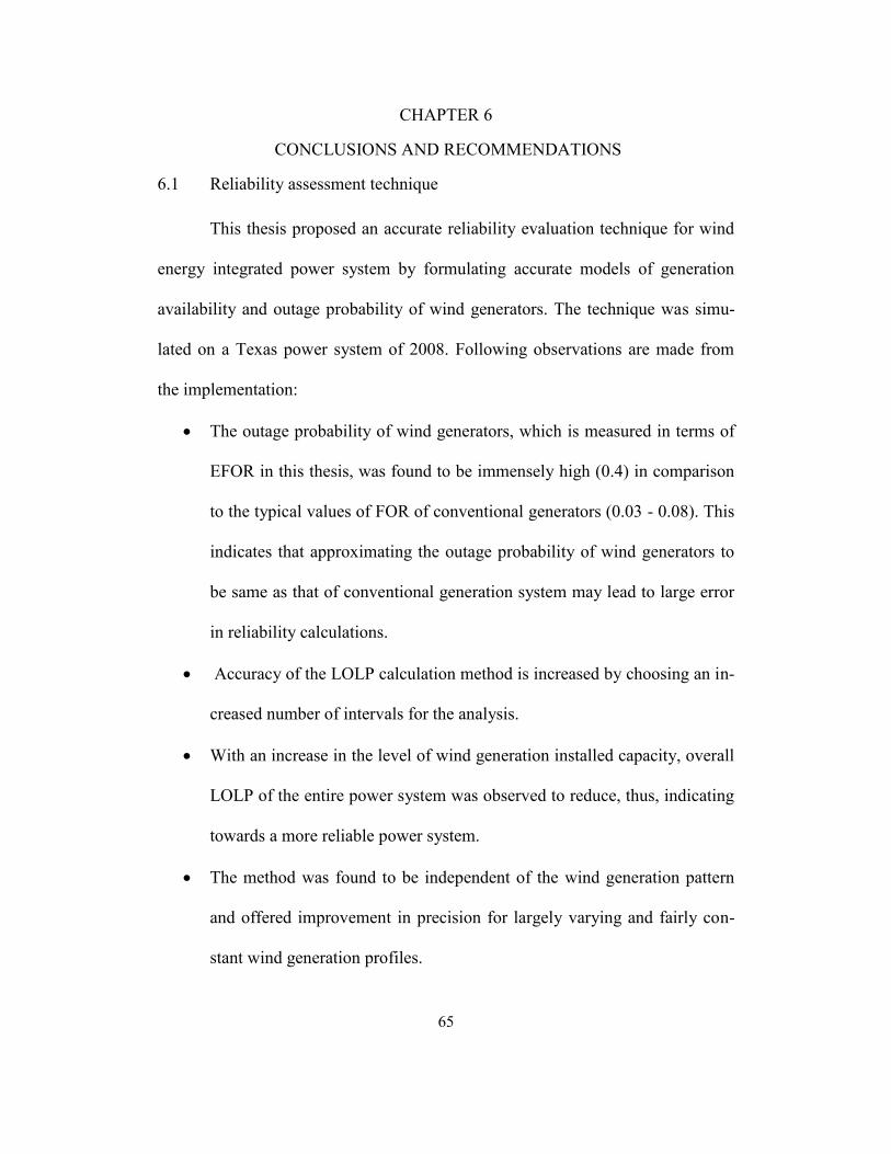
65

CHAPTER 6

CONCLUSIONS AND RECOMMENDATIONS

6.1 Reliability assessment technique

This thesis proposed an accurate reliability evaluation technique for wind

energy integrated power system by formulating accurate models of generation

availability and outage probability of wind generators. The technique was simu-

lated on a Texas power system of 2008. Following observations are made from

the implementation:

The outage probability of wind generators, which is measured in terms of

EFOR in this thesis, was found to be immensely high (0.4) in comparison

to the typical values of FOR of conventional generators (0.03 - 0.08). This

indicates that approximating the outage probability of wind generators to

be same as that of conventional generation system may lead to large error

in reliability calculations.

Accuracy of the LOLP calculation method is increased by choosing an in-

creased number of intervals for the analysis.

With an increase in the level of wind generation installed capacity, overall

LOLP of the entire power system was observed to reduce, thus, indicating

towards a more reliable power system.

The method was found to be independent of the wind generation pattern

and offered improvement in precision for largely varying and fairly con-

stant wind generation profiles.

66

It is recommended that while using the technique for a larger system, the

‘optimum’ number of intervals must be determined by iteration beyond which the

proposed LOLP calculation methodology offers no appreciable accuracy benefit.

Thus, computational space may be saved and system be simulated faster.

Lastly, with appropriate modifications, the method can be extended to

conduct reliability analysis of power system having a large amount of generation

contributed by varying sources of energy such as the solar generation.

6.2 GUI construction for a DFIG system

A GUI has been constructed to animatedly depict the operation of the

DFIG based wind generation system. The interface shows the behavior of power

flow, equivalent circuit, phasor diagram and maximum power point tracking

mechanism of the DFIG for the wind speed inputted by the user. The module has

been designed to work as a stand-alone software program without dependency on

MATLAB.

In addition to being accessible on any Windows based computer, the GUI

is a simplified representation of an extremely complicated wind generation tech-

nology. The tool could be used to educate as well as invoke interest among sci-

ence students about the promising potential of renewable power engineering.

In the future, the GUI may be made more versatile by adding features to

simulate the dynamic response of the machine and display the change in the elec-

trical waveforms with variation in operation conditions.

67

REFERENCES

[1] Ernest Orlando Lawrence Berkley National Laboratory, document available

on the topic “Understanding the cost of power interruptions to U.S. electricity

consumers,” available at:

http://certs.lbl.gov/pdf/55718.pdf

[2] S. Panya, T. Detmote, “Economic impact of power outage in Thailand: indus-

try perspectives,” International Conference on Energy and Sustainable Develop-

ment: Issues and Strategies, June 2010, pp. 1-7

[3] U.S. Energy Information Administration, document available on the topic

“U.S. electric net summer capacity, 2004 – 2008,” available at:

http://205.254.135.7/cneaf/solar.renewables/page/trends/table1_12.pdf

[4] American Wind Energy Association, article appearing on the topic “Industrial

statistics,” available at:

http://www.awea.org/learnabout/industry_stats/index.cfm

[5] U.S. Energy Information Administration, document available on the topic

“State electricity profiles,” available at:

http://205.254.135.7/electricity/

[6] U.S. Environmental Protection Agency, article appearing on the topic “Re-

newable portfolio standards fact sheet,” available at:

http://www.epa.gov/chp/state-policy/renewable_fs.html

[7] G.T. Heydt, V. Vittal, R. Ayyanar, “Power system operation and planning for

enhanced wind generation penetration – collaborative work force development,”

US Department of Energy grant award number: DE-EE0000535, October 2011

[8] R. Billinton, A.V. Jain, “Unit derating levels in spinning reserve studies,”

IEEE Transactions on Power Apparatus and Systems, July 1971, vol. PAS-90,

No. 4, pp. 1677-1687

[9] R. Billinton, A.V. Jain, C. MacGowan, “Effect of partial outage representation

in generation system planning studies,” IEEE Transactions on Power Apparatus

and Systems, September 1974, vol. PAS-93, No. 5, pp. 1252-1259

[10] R. Billinton, Y. Li, “Incorporating multi-state unit models in composite sys-

tem adequacy assessment,” International Conference on Probabilistic Methods

Applied to Power Systems, September 2004, pp. 70-75

[11] K.F. Schenk, R.B. Misra, S. Vassos, W. Wen, “A new method for the evalua-

tion of expected energy generation and loss of load probability,” IEEE Transac-

68

tions on Power Apparatus and Systems, February 1984, vol. PAS-103, No. 2, pp.

294-303

[12] G. Calabrese, “Generating reserve capacity determined by probability meth-

od,” Transactions of the American Institute of Electrical Engineers, January 1947,

vol. 66, No. 1, pp. 1439-1450

[13] A.K. Ayoub, J.D. Guy, A.D. Patton, “Evaluation and comparison of some

methods for calculating generating system reliability,” IEEE Transactions on

Power Apparatus and Systems, April 1970, vol. PAS-89, No. 4, pp. 537-544

[14] R. Karki, R. Billinton, “Cost-effective wind energy utilization for reliable

power supply,” IEEE Transactions on Energy Conversion, June 2004, vol. 19, No.

2, pp. 435-440

[15] R. Billinton and R. Karki, “Cost effective wind energy utilization for reliable

power supply,” IEEE Transactions on Energy Conversion, June 2004, vol. 19, No.

2, pp. 435–440

[16] R. Billinton, Y.C. Bagen, Y. Cui, “Reliability evaluation of small stand-alone

wind energy conversion systems using a time series simulation model,” IEEE

Proceedings on Generation, Transmission and Distribution, January 2003,

vol.150, No. 1, pp. 96-100

[17] P. Giorsetto, K.F. Utsurogi, “Development of a new procedure for reliability

modeling of wind turbine generators,” IEEE Transactions on Power Apparatus

and Systems, January 1983, vol. PAS-102, No. 1, pp. 134-143

[18] J.N. Jiang, C. Lin, T. Runolfsson, “A study of short-term impact of wind

generation on LOLP,” IEEE PES Conference on Transmission and Distribution,

April 2010, pp. 1-10

[19] ISO New England, article available on the topic “GADS/GADS equivalent

data,” available at:

http://www.iso-ne.com/genrtion_resrcs/gads/index.html

[20] A. Dimitrovski, K. Tomsovic, “Impact of wind generation uncertainty on

generating capacity adequacy,” International Conference on Probabilistic Meth-

ods Applied to Power Systems, June 2006, pp. 1-6

[21] Frede Blaabjerg, Zhe Chen, “Power electronics for modern wind turbines,”

First Edition, United States, Morgan and Claypool Publishers, 2007

[22] D. McSwiggan, T. Littler, D.J. Morrow, J. Kennedy, “A study of tower shad-

ow effect on fixed-speed wind turbines,” 43rd

International Universities Power

Engineering Conference, September 2008, pp. 1-5

69

[23] National Renewable Energy Laboratory, document available on the topic

“The history and state of the art of variable-speed wind turbine technolo-

gy,” available at:

www.nrel.gov/docs/fy01osti/28607.pdf

[24] L. Dusonchet, F. Massaro, E. Telaretti, “Wind turbine mechanical character-

istics and grid parameters influence on the transient voltage stability of a fixed

speed wind turbine,” 43rd

International Universities Power Engineering Confer-

ence, September 2008, pp. 1-5

[25] Y. Ashkhane, “A new approach to improve voltage stability in a network

with fixed speed wind turbines,” 19th

Iranian Conference on Electrical Engineer-

ing, May 2011, pp. 1-6

[26] G. Jinxia, X. Da, Z. Yanchi, “A new excitation regulating and harmonic

eliminating equipment for fixed speed fixed pitch wind turbines,” International

Conference on Electrical Machines and Systems, October 2008, pp. 2556 – 2560

[27] A. Sinha, D. Kumar, D. Kumar, P. Samuel, R. Gupta, “A two-stage converter

based controller for a stand alone wind energy system used for remote applica-

tions,” 30th

IEEE International Conference on Telecommunication Energy, Sep-

tember 2008, pp. 1-5

[28] D. Fujin, C. Zhe, “A new structure based on cascaded multilevel converter

for variable speed wind turbine,” 36th

Annual Conference on IEEE Industrial

Electronics Society, November 2010, pp. 3167 - 3172

[29] H. Nikkhajoei, R.H. Lasseter, “Power quality enhancement of a wind-turbine

generator under variable wind speeds using matrix converter,” Power Electronics

Specialist Conference, June 2008, pp. 1755 - 1761

[30] H. Karimi-Davijani, A. Sheikholeslami, R. Ahmadi, H. Livani, “Active and

reactive power control of DFIG using SVPWM converter,” 43rd

International

Universities Power Engineering Conference, September 2008, pp. 1-5

[31] O. Duan, L. Zhang, L. Zhang, “A fault detection and tolerant scheme for

back-to-back converters in DFIG-based wind power generation systems,” 3rd

In-

ternational Conference on Advanced Computer Theory and Engineering, August

2010, vol. 3, pp. 95 - 99

[32] Wikipedia, article appearing on the topic “Reliability engineering,” available

at:

http://en.wikipedia.org/wiki/Reliability_engineering

70

[33] Virginia Polytechnic Institute, document available on the topic “Power sys-

tem reliability analysis with distributed generators,” available at:

http://scholar.lib.vt.edu/theses/available/etd-05162003-

090532/unrestricted/Power_System.pdf

[34] Massachusetts Institute of Technology, document available on the topic “The

value of reliability on power systems- pricing operating reserves,” available at:

http://web.mit.edu/energylab/www/pubs/el99-005wp.pdf

[35] G. T. Heydt, “Lecture notes on Power Systems Operation and Planning,” Ar-

izona State University, Fall 2010

[36] K. Malmedal, P.K. Sen, “A better understanding of load and loss factors,”

Industry Applications Society Annual Meeting, October 2008, pp. 1-6

[37] M. O. M Mahmoud, M. Jaidane-Saidane, J. Souissi, N. Hizaoui, “Modeling

of the load duration curve using the asymmetric generalized Gaussian distribu-

tion: case of the Tunisian power system,” Power and Energy Society General

Meeting on Conversion and Delivery of Electrical Energy in the 21st century, July

2008, pp.1-7

[38] M. O. M Mahmoud, M. Jaidane-Saidane, J. Souissi, N. Hizaoui, “The mix-

ture of generalized Gaussian model for modeling of the load duration curve: case

of the Tunisian power system,” 14th

IEEE Mediterranean Electrotechnical Con-

ference (MELECON), May 2008, pp. 774 – 779

[39] National Climatic Data Center, document available on the topic “Wind-

average wind speed (MPH)” available at:

http://lwf.ncdc.noaa.gov/oa/climate/online/ccd/avgwind.html

[40] Dr. Yih-huei Wan, National Renewable Electric Laboratory, private commu-

nication, April 27, 2011

[41] S. Tehrani, T. E. Weymouth, B. Schunck, “Interpolating cubic spline con-

tours by minimizing second derivative discontinuity,” 3rd

International Confer-

ence on Computer Vision, December 1990, pp. 713 – 716

[42] National Oceanic and Atmospheric Association, article available on the topic

“NOAA recorded average wind speed data through 2001,” available at:

http://www.berner.com/sales/energy_windspeed.html

[43] U.S Energy Information Administration, article available on the topic

“Electricity generating capacity,” available at:

http://www.eia.gov/electricity/capacity

71

[44] Wikipedia, article available on the topic “Renewable portfolio standard,”

available at:

http://en.wikipedia.org/wiki/Renewable_portfolio_standard

[45] Electric Reliability Council of Texas, document available on topic “Load,”

available at:

http://www.ercot.com/gridinfo/load/

[46] U.S. Energy Information Administration, document available on topic “State

total electric power industry net summer capacity, by Energy Source, 2004 –

2008,” available at:

http://www.google.com/url?sa=t&rct=j&q=rspt02tx&source=web&cd=1&ved=0

CCAQFjAA&url=http%3A%2F%2Fwww.eia.gov%2Fcneaf%2Fsolar.renewables

%2Fpage%2Fstate_profiles%2Frspt02tx.xls&ei=kyQST9vCNemriQLV4vm_DQ

&usg=AFQjCNFriHZhlbA8k9flIPDg_kqUGSDwgA

[47] ISO New England, article available on the topic “ISO New England EFORd

class averages from NERC brochure,” available at:

http://www.iso-ne.com/genrtion_resrcs/gads/class_avg_2009.pdf

[48] Thomas Ackerman, “Wind power in power systems,” First Edition, Sweden,

John Wiley and Sons Limited, 2005

[49] Siemens Corporation, article available on the topic “Introduction to generic

wind turbine generator models,” available at:

https://www.pti-us.com/pti/company/enewsletter/2011may/pdfs/Introduction

%20to%20Generic%20Wind%20Models.pdf

[50] Brendan Fox, Damian Flynn, et al., “Wind power integration connection and

system operational aspects,” First Edition, United Kingdom, The Institution of

Engineering and Technology, 2007

[51] Wikipedia, article appearing on the topic “Doubly fed electric machine,”

available at:

http://en.wikipedia.org/wiki/Doubly_fed_electric_machine

[52] User-Defined Model Manual for DSA Tools available at the Electrical Power

Engineering Department at Arizona State University

[53] R. Ayyanar, “Lecture notes on Electrical Machines,” Arizona State Universi-

ty, Fall 2011

[54] eWashtenaw, document available on the topic “Wind turbine brochures,”

available at:

http://www.ewashtenaw.org/government/departments/planning_environment/plan

ning/wind_power/Monthly%20Data_Reports/Attachment_1.pdf

72

APPENDIX A

MATLAB CODE FOR RELIABILITY STUDY IMPLEMENTATION ON

TEXAS POWER SYSTEM

73

%%%%%%%%%%%%%%%%%%%%%%%%%%%%%%%%%%%%%%%%%%%%%%%%%%%%%%%%%%%%%%%%%

%Author: Anubhav Sinha, Arizona State University

%Faculty Advisor: Dr. Gerald T. Heydt, Dr. Vijay Vittal, Dr. Raja

Ayyanar, Arizona State University

%2011-2012

%%%%%%%%%%%%%%%%%%%%%%%%%%%%%%%%%%%%%%%%%%%%%%%%%%%%%%%%%%%%%%%%%

Master_Dec23_08.m

% This is the central file that loads the LDC data and calls the

COT function

total_rows=8760;

global Load L1

L1=< 8760x1 matrix of actual hourly load data of Texas in 2008>’

global Marker

Marker(1,1)=0;

Marker(1,2)=0;

cou=2;

cou_2=1;

watch_1=0;

for(i=1:1:10)

i;

G=i*(max(L)/10);

watch_1=0;

cou=2;

while (watch_1==0)

e1=G-L(cou);

e2=G-(L(cou-1));

cou=cou+1;

if (((e1>0)&&(e2<=0))||((e1>=0)&&(e2<0)))

watch_1=1;

end

74

end

Marker(i,1)=G;

Marker(i,2)=cou-1;

end

Marker; %Complete Marker matrix

COT_Dec23_08() %Calling function to generate COT

COT_Dec23_08.m

% This is the function that constructs the COT for the test case

10-generator system

function COT_Dec23_08()

states=12;

%%%%%%%%%%%%%%%%%%%%%%%%%%%%%%%%%%%%%%%%%%%%%%%%%%%%%%%%%%%%%%%%%

x=10; % x indicates the total number of MW entries allowed in

the input

Coal1=[5.19 0.0718]; % Two Coal generators.

Coal2=[15 0.0621];

NG1=[15.86 0.0747]; % Three NG generators

NG2=[25 0.0633];

NG3=[30 0.0548];

Nuclear1=[2.36 0.0273]; % Two Nuclear-reactor based generation

Nuclear2=[2.5 0.0273];

Total_load = [4217.3 4383.3 4377.9 4333.2 4251.1 4122.9 4139.7

4340.5 4520.3 4185.7 4232.3 3986.1 3783 3407.2 3527.6 3538.9

3767.5 3841.4 4062 3825.4 3672.2 3378.9 3216 2656.5];

test_case=[4 6 8 12 24 32 48 72 96];

%%%%%%%%%%%%%%%%%%%%%%%%%%%%%%%%%%%%%%%%%%%%%%%%%%%%%%%%%%%%%%%%%

if(states==4) %Number of states

dataspaces = linspace(0,23,24);

75

samples = 0:6:23;

p_4 = pchip(dataspaces,Total_load,samples);

G(1).Hours=[6 6 6 6];

G(2).Hours=[6 6 6 6];

G(3).Hours=[6 6 6 6];

G(1).Ld=(5/12)*p_4;

G(2).Ld=(4/12)*p_4;

G(3).Ld=(3/12)*p_4;

G(1).FOR=p_4/7.43/1000;

G(2).FOR=p_4/7.43/1000;

G(3).FOR=p_4/7.43/1000;

end

%%%%%%%%%%%%%%%%%%%%%%%%%%%%%%%%%%%%%%%%%%%%%%%%%%%%%%%%%%%%%%%%%

if(states==6) %Number of states EQUAL SPACED

dataspaces = linspace(0,23,24);

samples = 0:4:23;

p_6 = pchip(dataspaces,Total_load,samples);

G(1).Hours=[4 4 4 4 4 4];

G(2).Hours=[4 4 4 4 4 4];

G(3).Hours=[4 4 4 4 4 4];

G(1).Ld=(5/12)*p_6;

G(2).Ld=(4/12)*p_6;

G(3).Ld=(3/12)*p_6;

G(1).FOR=p_6/7.43/1000;

G(2).FOR=p_6/7.43/1000;

G(3).FOR=p_6/7.43/1000;

end

%%%%%%%%%%%%%%%%%%%%%%%%%%%%%%%%%%%%%%%%%%%%%%%%%%%%%%%%%%%%%%%%%

76

if(states==8) %Number of states

dataspaces = linspace(0,23,24);

samples = 0:3:24;

p_8 = pchip(dataspaces,Total_load,samples);

plot(dataspaces,Total_load,'o ',samples,p_8,'+')

G(1).Hours=[3 3 3 3 3 3 3 3];

G(2).Hours=[3 3 3 3 3 3 3 3];

G(3).Hours=[3 3 3 3 3 3 3 3];

G(1).Ld=(5/12)*p_8;

G(2).Ld=(4/12)*p_8;

G(3).Ld=(3/12)*p_8;

G(1).FOR=p_8/7.43/1000;

G(2).FOR=p_8/7.43/1000;

G(3).FOR=p_8/7.43/1000;

end

%%%%%%%%%%%%%%%%%%%%%%%%%%%%%%%%%%%%%%%%%%%%%%%%%%%%%%%%%%%%%%%%%

if(states==12) %Number of states

dataspaces = linspace(0,23,24);

samples = 0:2:24;

p_12 = pchip(dataspaces,Total_load,samples);

plot(dataspaces,Total_load,'o ',samples,p_12,'+')

G(1).Hours=[2 2 2 2 2 2 2 2 2 2 2 2];

G(2).Hours=[2 2 2 2 2 2 2 2 2 2 2 2];

G(3).Hours=[2 2 2 2 2 2 2 2 2 2 2 2];

G(1).Ld=(5/12)*p_12;

G(2).Ld=(4/12)*p_12;

G(3).Ld=(3/12)*p_12;

G(1).FOR=p_12/7.43/1000;

G(2).FOR=p_12/7.43/1000;

77

G(3).FOR=p_12/7.43/1000;

end

%%%%%%%%%%%%%%%%%%%%%%%%%%%%%%%%%%%%%%%%%%%%%%%%%%%%%%%%%%%%%%%%%

if(states==18) %Number of states

G(1).Hours=[1 1 1 1 1 1 1 1 1 1 1 1 1 1 6 1 1 1];

G(2).Hours=[1 1 1 1 1 1 1 1 1 1 1 1 1 1 6 1 1 1];

G(3).Hours=[1 1 1 1 1 1 1 1 1 1 1 1 1 1 6 1 1 1];

G(1).Ld=[1.145 1.167 1.146 1.146 1.125 1.104 1.0833 1.042 0.9375

0.833 0.833 0.667 0.521 0.375 0.7083 1.0833 1.0833 0.9167];

G(2).Ld=[0.9167 0.933 0.9166 0.9166 0.9 0.8833 0.866 0.833 0.75

0.667 0.667 0.533 0.4167 0.3 0.5667 0.866 0.866 0.733];

G(3).Ld=[0.6875 0.7 0.6875 0.6875 0.675 0.6625 0.65 0.625 0.5625

0.5 0.5 0.4 0.3125 0.225 0.425 0.65 0.65 0.55];

G(1).FOR=[0.6395 0.6512 0.6395 0.6395 0.6279 0.6163 0.6046 0.5814

0.5233 0.4651 0.4651 0.3721 0.2907 0.2093 0.3953 0.6046 0.6046

0.5116];

G(2).FOR=[0.6395 0.6512 0.6395 0.6395 0.6279 0.6163 0.6046 0.5814

0.5233 0.4651 0.4651 0.3721 0.2907 0.2093 0.3953 0.6046 0.6046

0.5116];

G(3).FOR=[0.6395 0.6512 0.6395 0.6395 0.6279 0.6163 0.6046 0.5814

0.5233 0.4651 0.4651 0.3721 0.2907 0.2093 0.3953 0.6046 0.6046

0.5116];

end

%%%%%%%%%%%%%%%%%%%%%%%%%%%%%%%%%%%%%%%%%%%%%%%%%%%%%%%%%%%%%%%%%

if(states==24) %Number of states

dataspaces = linspace(0,23,24);

samples = 0:1:24;

p_24 = pchip(dataspaces,Total_load,samples);

p_24(24)=0.5*(p_24(23)+p_24(1));

78

G(1).Hours=[1 1 1 1 1 1 1 1 1 1 1 1 1 1 1 1 1 1 1 1 1 1 1 1];

G(2).Hours=[1 1 1 1 1 1 1 1 1 1 1 1 1 1 1 1 1 1 1 1 1 1 1 1];

G(3).Hours=[1 1 1 1 1 1 1 1 1 1 1 1 1 1 1 1 1 1 1 1 1 1 1 1];

G(1).Ld=(5/12)*p_24;

G(2).Ld=(4/12)*p_24;

G(3).Ld=(3/12)*p_24;

G(1).FOR=p_24/7.43/1000;

G(2).FOR=p_24/7.43/1000;

G(3).FOR=p_24/7.43/1000;

end

%%%%%%%%%%%%%%%%%%%%%%%%%%%%%%%%%%%%%%%%%%%%%%%%%%%%%%%%%%%%%%%%%

if(states==32) %Number of states

dataspaces = linspace(0,23,24);

samples = 0:.75:23.25;

p_32 = pchip(dataspaces,Total_load,samples);

p_32(32)=0.5*(p_32(31)+p_32(1));

G(1).Hours=[0.75 0.75 0.75 0.75 0.75 0.75 0.75 0.75 0.75 0.75

0.75 0.75 0.75 0.75 0.75 0.75 0.75 0.75 0.75 0.75 0.75 0.75 0.75

0.75 0.75 0.75 0.75 0.75 0.75 0.75 0.75 0.75];

G(2).Hours=[0.75 0.75 0.75 0.75 0.75 0.75 0.75 0.75 0.75 0.75

0.75 0.75 0.75 0.75 0.75 0.75 0.75 0.75 0.75 0.75 0.75 0.75 0.75

0.75 0.75 0.75 0.75 0.75 0.75 0.75 0.75 0.75];

G(3).Hours=[0.75 0.75 0.75 0.75 0.75 0.75 0.75 0.75 0.75 0.75

0.75 0.75 0.75 0.75 0.75 0.75 0.75 0.75 0.75 0.75 0.75 0.75 0.75

0.75 0.75 0.75 0.75 0.75 0.75 0.75 0.75 0.75];

G(1).Ld=(5/12)*p_32;

G(2).Ld=(4/12)*p_32;

G(3).Ld=(3/12)*p_32;

G(1).FOR=p_32/7.43/1000;

79

G(2).FOR=p_32/7.43/1000;

G(3).FOR=p_32/7.43/1000;

end

%%%%%%%%%%%%%%%%%%%%%%%%%%%%%%%%%%%%%%%%%%%%%%%%%%%%%%%%%%%%%%%%%

if(states==48) %Number of states

dataspaces = linspace(0,23,24);

samples = 0:.5:23.5;

p_48 = pchip(dataspaces,Total_load,samples);

p_48(48)=0.5*(p_48(47)+p_48(1));

%s = spline(x,y,t);

%plot(dataspaces,Total_load,'o ',samples,p_48,'+')

%legend('data','pchip','spline',4)

G(1).Hours=[0.5 0.5 0.5 0.5 0.5 0.5 0.5 0.5 0.5 0.5 0.5 0.5 0.5

0.5 0.5 0.5 0.5 0.5 0.5 0.5 0.5 0.5 0.5 0.5 0.5 0.5 0.5 0.5 0.5

0.5 0.5 0.5 0.5 0.5 0.5 0.5 0.5 0.5 0.5 0.5 0.5 0.5 0.5 0.5 0.5

0.5 0.5 0.5];

G(2).Hours=[0.5 0.5 0.5 0.5 0.5 0.5 0.5 0.5 0.5 0.5 0.5 0.5 0.5

0.5 0.5 0.5 0.5 0.5 0.5 0.5 0.5 0.5 0.5 0.5 0.5 0.5 0.5 0.5 0.5

0.5 0.5 0.5 0.5 0.5 0.5 0.5 0.5 0.5 0.5 0.5 0.5 0.5 0.5 0.5 0.5

0.5 0.5 0.5];

G(3).Hours=[0.5 0.5 0.5 0.5 0.5 0.5 0.5 0.5 0.5 0.5 0.5 0.5 0.5

0.5 0.5 0.5 0.5 0.5 0.5 0.5 0.5 0.5 0.5 0.5 0.5 0.5 0.5 0.5 0.5

0.5 0.5 0.5 0.5 0.5 0.5 0.5 0.5 0.5 0.5 0.5 0.5 0.5 0.5 0.5 0.5

0.5 0.5 0.5];

G(1).Ld=(5/12)*p_48;

G(2).Ld=(4/12)*p_48;

G(3).Ld=(3/12)*p_48;

G(1).FOR=p_48/7.43/1000;

G(2).FOR=p_48/7.43/1000;

G(3).FOR=p_48/7.43/1000;

80

end

%%%%%%%%%%%%%%%%%%%%%%%%%%%%%%%%%%%%%%%%%%%%%%%%%%%%%%%%%%%%%%%%%

if(states==72) %Number of states

dataspaces = linspace(0,23,24);

samples = 0:0.3333:23.999;

p_72 = pchip(dataspaces,Total_load,samples);

%p_72(72)=0.5*(p_72(71)+p_72(1));

%s = spline(x,y,t);

%plot(dataspaces,Total_load,'o ',samples,p_72,'+')

%legend('data','pchip','spline',4)

G(1).Hours=[0.333 0.333 0.333 0.333 0.333 0.333 0.333 0.333 0.333

0.333 0.333 0.333 0.333 0.333 0.333 0.333 0.333 0.333 0.333 0.333

0.333 0.333 0.333 0.333 0.333 0.333 0.333 0.333 0.333 0.333 0.333

0.333 0.333 0.333 0.333 0.333 0.333 0.333 0.333 0.333 0.333 0.333

0.333 0.333 0.333 0.333 0.333 0.333 0.333 0.333 0.333 0.333 0.333

0.333 0.333 0.333 0.333 0.333 0.333 0.333 0.333 0.333 0.333 0.333

0.333 0.333 0.333 0.333 0.333 0.333 0.333 0.333];

G(2).Hours=G(1).Hours;

G(3).Hours=G(2).Hours;

G(1).Ld=(5/12)*p_72;

G(2).Ld=(4/12)*p_72;

G(3).Ld=(3/12)*p_72;

G(1).FOR=p_72/7.43/1000;

G(2).FOR=p_72/7.43/1000;

G(3).FOR=p_72/7.43/1000;

end

%%%%%%%%%%%%%%%%%%%%%%%%%%%%%%%%%%%%%%%%%%%%%%%%%%%%%%%%%%%%%%%%%

if(states==96) %Number of states

dataspaces = linspace(0,23,24);

samples = 0:0.25:23.999;

p_96 = pchip(dataspaces,Total_load,samples);

81

plot(dataspaces,Total_load,'o ',samples,p_96,'+')

G(1).Hours=[0.25 0.25 0.25 0.25 0.25 0.25 0.25 0.25 0.25 0.25

0.25 0.25 0.25 0.25 0.25 0.25 0.25 0.25 0.25 0.25 0.25 0.25 0.25

0.25 0.25 0.25 0.25 0.25 0.25 0.25 0.25 0.25 0.25 0.25 0.25 0.25

0.25 0.25 0.25 0.25 0.25 0.25 0.25 0.25 0.25 0.25 0.25 0.25 0.25

0.25 0.25 0.25 0.25 0.25 0.25 0.25 0.25 0.25 0.25 0.25 0.25 0.25

0.25 0.25 0.25 0.25 0.25 0.25 0.25 0.25 0.25 0.25 0.25 0.25 0.25

0.25 0.25 0.25 0.25 0.25 0.25 0.25 0.25 0.25 0.25 0.25 0.25 0.25

0.25 0.25 0.25 0.25 0.25 0.25 0.25 0.25];

G(2).Hours=G(1).Hours;

G(3).Hours=G(2).Hours;

G(1).Ld=(5/12)*p_96;

G(2).Ld=(4/12)*p_96;

G(3).Ld=(3/12)*p_96;

G(1).FOR=p_96/7.43/1000;

G(2).FOR=p_96/7.43/1000;

G(3).FOR=p_96/7.43/1000;

end

%%%%%%%%%%%%%%%%%%%%%%%%%%%%%%%%%%%%%%%%%%%%%%%%%%%%%%%%%%%%%%%%%

if(states==144) %Number of states

dataspaces = linspace(0,23,24);

samples = 0:0.16667:23.999;

p_144 = pchip(dataspaces,Total_load,samples);

G(1).Hours=[0.16667 0.16667 0.16667 0.16667 0.16667 0.16667

0.16667 0.16667 0.16667 0.16667 0.16667 0.16667 0.16667 0.16667

0.16667 0.16667 0.16667 0.16667 0.16667 0.16667 0.16667 0.16667

0.16667 0.16667 0.16667 0.16667 0.16667 0.16667 0.16667 0.16667

0.16667 0.16667 0.16667 0.16667 0.16667 0.16667 0.16667 0.16667

0.16667 0.16667 0.16667 0.16667 0.16667 0.16667 0.16667 0.16667

82

0.16667 0.16667 0.16667 0.16667 0.16667 0.16667 0.16667 0.16667

0.16667 0.16667 0.16667 0.16667 0.16667 0.16667 0.16667 0.16667

0.16667 0.16667 0.16667 0.16667 0.16667 0.16667 0.16667 0.16667

0.16667 0.16667 0.16667 0.16667 0.16667 0.16667 0.16667 0.16667

0.16667 0.16667 0.16667 0.16667 0.16667 0.16667 0.16667 0.16667

0.16667 0.16667 0.16667 0.16667 0.16667 0.16667 0.16667 0.16667

0.16667 0.16667 0.16667 0.16667 0.16667 0.16667 0.16667 0.16667

0.16667 0.16667 0.16667 0.16667 0.16667 0.16667 0.16667 0.16667

0.16667 0.16667 0.16667 0.16667 0.16667 0.16667 0.16667 0.16667

0.16667 0.16667 0.16667 0.16667 0.16667 0.16667 0.16667 0.16667

0.16667 0.16667 0.16667 0.16667 0.16667 0.16667 0.16667 0.16667

0.16667 0.16667 0.16667 0.16667 0.16667 0.16667 0.16667 0.16667

0.16667 0.16667];

G(2).Hours=G(1).Hours;

G(3).Hours=G(2).Hours;

G(1).Ld=(5/12)*p_144;

G(2).Ld=(4/12)*p_144;

G(3).Ld=(3/12)*p_144;

G(1).FOR=p_144/7.43/1000;

G(2).FOR=p_144/7.43/1000;

G(3).FOR=p_144/7.43/1000;

end

%%%%%%%%%%%%%%%%%%%%%%%%%%%%%%%%%%%%%%%%%%%%%%%%%%%%%%%%%%%%%%%%%

G4=Coal1;

G5=Coal2;

%%%%%%%%%%%%%%%%%%

G6=NG1;

G7=NG2;

83

G8=NG3;

%%%%%%%%%%%%%%%%%%

G9=Nuclear1;

G10=Nuclear2;

%%%%%%%%%%%%%%%%%%%%%%%%%%%%%%%%%%%%%%%%%%%%%%%%%%%%%%%%%%%%%%%%%

%%%%%%%

for (d=1:1:3) %Calculating Equivalent load

Sum=0;

for(c=1:1:states)

Sum=Sum+(G(d).Hours(c))*(G(d).Ld(c));

end

M(d)= Sum/24*0.001;

end

for (d=1:1:3) %Calculating Equivalent load

Sum=0;

for(c=1:1:states)

Sum=Sum+(G(d).Hours(c))*(G(d).FOR(c));

end

P(d)= Sum/24;

end

%%%%%%%%%%%%%%%%%%%%%%%%%%%%%%%%%%%%%%%%%%%%%%%%%%%%

M(4)=G4(1,1); %Tabulating generation data

M(5)=G5(1,1);

M(6)=G6(1,1);

M(7)=G7(1,1);

M(8)=G8(1,1);

M(9)=G9(1,1);

M(10)=G10(1,1);

M;

84

P(4)=G4(1,2); % Tabulating the outage probability

P(5)=G5(1,2);

P(6)=G6(1,2);

P(7)=G7(1,2);

P(8)=G8(1,2);

P(9)=G9(1,2);

P(10)=G10(1,2);

P;

%%%%%%%%%%%%%%%%%%%%%%%%%%%%%%%%%%%%%

%Eliminating zero values in 'm' array

%%%%%%%%%%%%%%%%%%%%%%%%%%%%%%%%%%%%%%

c=1;

for i=1:1:x

if (M(i)~=0)

m(c)=M(i); %Transfer the non-zero entries to 'm' array

p(c)=P(i); %Save the corresponding FOR in 'p' array

c=c+1; %c calculates the number of non-zero MW values

end

end

c=c-1;

m;

p;

%%%%%%%%%%%%%%%%%%%%%%%%%%%%%%%

%Generating Binary Table g

%%%%%%%%%%%%%%%%%%%%%%%%%%%%%%%

i=0;

j=c;

for i=0:1:((2^c)-1)

for k=1:1:c

g((i+1),k)=bitget(i,j);

j=j-1;

end

i=i+1;

j=c;

85

end

g;

%%%%%%%%%%%%%%%%%%%%%%%%%%%%%%%%%%%%

%Bitwise multipication of m and g

%%%%%%%%%%%%%%%%%%%%%%%%%%%%%%%%%%%%

for j=1:1:(2^c)

for i=1:1:c

k(j,i)=m(i)*g(j,i);

end

end

k;

%%%%%%%%%%%%%%%%%%%%%%%%%%%%%%%%%

%Obtain 'Load' column of COT

%%%%%%%%%%%%%%%%%%%%%%%%%%%%%%%%%

for i=1:1:(2^c)

r(i,1)=0;

end

for j=1:1:(2^c)

for i=1:1:c

r(j,1)=k(j,i)+r(j,1);

end

end

r;

%%%%%%%%%%%%%%%%%%%%%%%%%%%%%%%%%%%%%

%Generate table of FOR multiplication

%%%%%%%%%%%%%%%%%%%%%%%%%%%%%%%%%%%%%

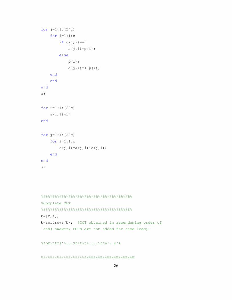
86

for j=1:1:(2^c)

for i=1:1:c

if g(j,i)==0

a(j,i)=p(i);

else

p(i);

a(j,i)=1-p(i);

end

end

end

a;

for i=1:1:(2^c)

s(i,1)=1;

end

for j=1:1:(2^c)

for i=1:1:c

s(j,1)=a(j,i)*s(j,1);

end

end

s;

%%%%%%%%%%%%%%%%%%%%%%%%%%%%%%%%%%%%%%%%

%Complete COT

%%%%%%%%%%%%%%%%%%%%%%%%%%%%%%%%%%%%%%%%

b=[r,s];

b=sortrows(b); %COT obtained in ascendening order of

load(However, FORs are not added for same load).

%fprintf('%13.9f\t\t%13.15f\n', b')

%%%%%%%%%%%%%%%%%%%%%%%%%%%%%%%%%%%%%%%%%

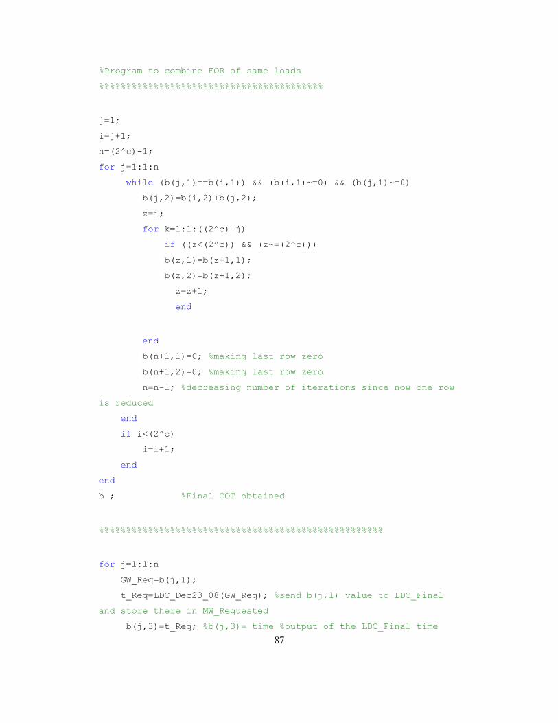
87

%Program to combine FOR of same loads

%%%%%%%%%%%%%%%%%%%%%%%%%%%%%%%%%%%%%%%%%

j=1;

i=j+1;

n=(2^c)-1;

for j=1:1:n

while (b(j,1)==b(i,1)) && (b(i,1)~=0) && (b(j,1)~=0)

b(j,2)=b(i,2)+b(j,2);

z=i;

for k=1:1:((2^c)-j)

if ((z<(2^c)) && (z~=(2^c)))

b(z,1)=b(z+1,1);

b(z,2)=b(z+1,2);

z=z+1;

end

end

b(n+1,1)=0; %making last row zero

b(n+1,2)=0; %making last row zero

n=n-1; %decreasing number of iterations since now one row

is reduced

end

if i<(2^c)

i=i+1;

end

end

b ; %Final COT obtained

%%%%%%%%%%%%%%%%%%%%%%%%%%%%%%%%%%%%%%%%%%%%%%%%%%%%

for j=1:1:n

GW_Req=b(j,1);

t_Req=LDC_Dec23_08(GW_Req); %send b(j,1) value to LDC_Final

and store there in MW_Requested

b(j,3)=t_Req; %b(j,3)= time %output of the LDC_Final time

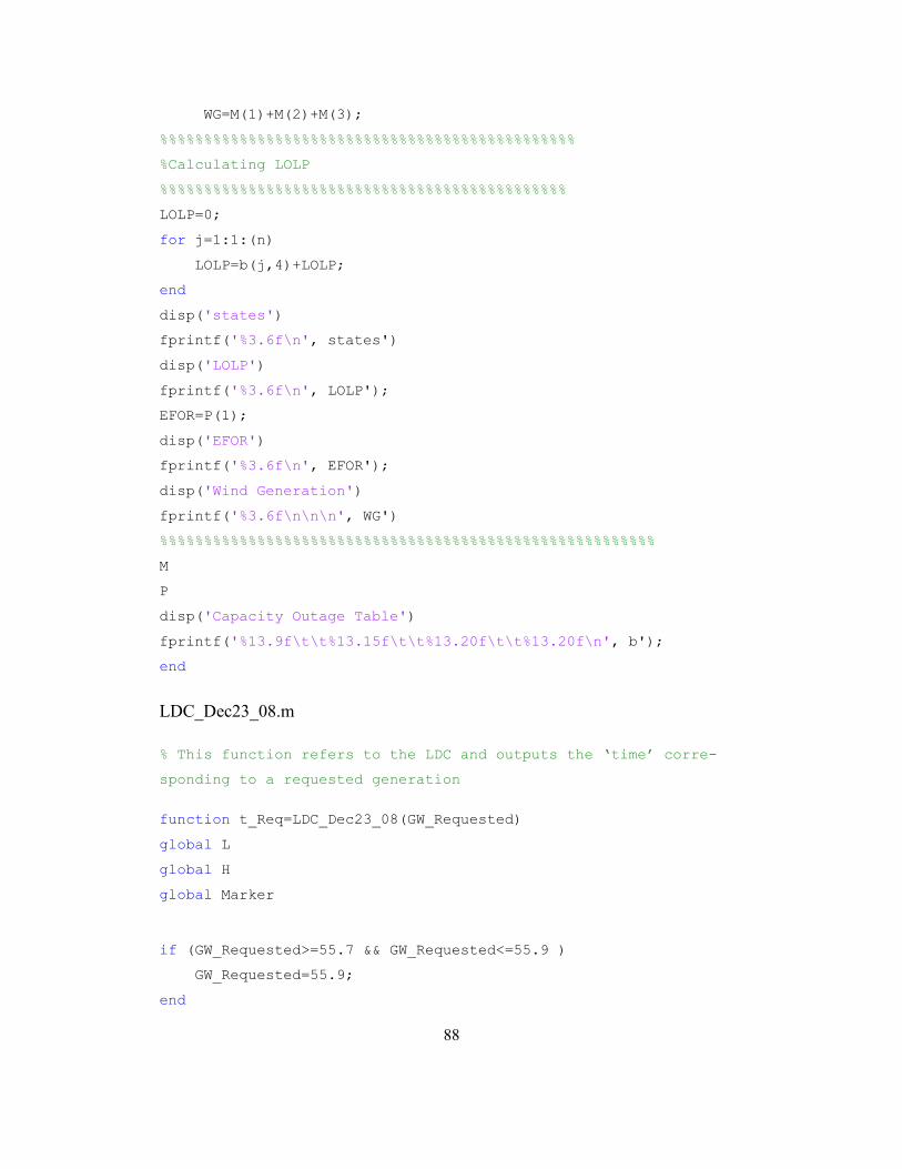
88

WG=M(1)+M(2)+M(3);

%%%%%%%%%%%%%%%%%%%%%%%%%%%%%%%%%%%%%%%%%%%%%%%

%Calculating LOLP

%%%%%%%%%%%%%%%%%%%%%%%%%%%%%%%%%%%%%%%%%%%%%%

LOLP=0;

for j=1:1:(n)

LOLP=b(j,4)+LOLP;

end

disp('states')

fprintf('%3.6f\n', states')

disp('LOLP')

fprintf('%3.6f\n', LOLP');

EFOR=P(1);

disp('EFOR')

fprintf('%3.6f\n', EFOR');

disp('Wind Generation')

fprintf('%3.6f\n\n\n', WG')

%%%%%%%%%%%%%%%%%%%%%%%%%%%%%%%%%%%%%%%%%%%%%%%%%%%%%%%%

M

P

disp('Capacity Outage Table')

fprintf('%13.9f\t\t%13.15f\t\t%13.20f\t\t%13.20f\n', b');

end

LDC_Dec23_08.m

% This function refers to the LDC and outputs the ‘time’ corre-

sponding to a requested generation

function t_Req=LDC_Dec23_08(GW_Requested)

global L

global H

global Marker

if (GW_Requested>=55.7 && GW_Requested<=55.9 )

GW_Requested=55.9;

end

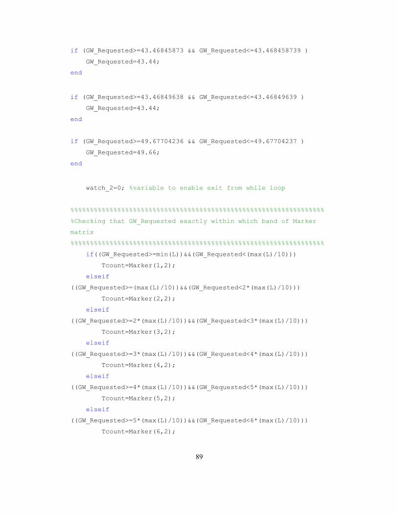
89

if (GW_Requested>=43.46845873 && GW_Requested<=43.468458739 )

GW_Requested=43.44;

end

if (GW_Requested>=43.46849638 && GW_Requested<=43.46849639 )

GW_Requested=43.44;

end

if (GW_Requested>=49.67704236 && GW_Requested<=49.67704237 )

GW_Requested=49.66;

end

watch_2=0; %variable to enable exit from while loop

%%%%%%%%%%%%%%%%%%%%%%%%%%%%%%%%%%%%%%%%%%%%%%%%%%%%%%%%%%%%%%%%%

%Checking that GW_Requested exactly within which band of Marker

matrix

%%%%%%%%%%%%%%%%%%%%%%%%%%%%%%%%%%%%%%%%%%%%%%%%%%%%%%%%%%%%%%%%%

if((GW_Requested>=min(L))&&(GW_Requested<(max(L)/10)))

Tcount=Marker(1,2);

elseif

((GW_Requested>=(max(L)/10))&&(GW_Requested<2*(max(L)/10)))

Tcount=Marker(2,2);

elseif

((GW_Requested>=2*(max(L)/10))&&(GW_Requested<3*(max(L)/10)))

Tcount=Marker(3,2);

elseif

((GW_Requested>=3*(max(L)/10))&&(GW_Requested<4*(max(L)/10)))

Tcount=Marker(4,2);

elseif

((GW_Requested>=4*(max(L)/10))&&(GW_Requested<5*(max(L)/10)))

Tcount=Marker(5,2);

elseif

((GW_Requested>=5*(max(L)/10))&&(GW_Requested<6*(max(L)/10)))

Tcount=Marker(6,2);

90

elseif

((GW_Requested>=6*(max(L)/10))&&(GW_Requested<7*(max(L)/10)))

Tcount=Marker(7,2);

elseif

((GW_Requested>=7*(max(L)/10))&&(GW_Requested<8*(max(L)/10)))

Tcount=Marker(8,2);

elseif

((GW_Requested>=8*(max(L)/10))&&(GW_Requested<9*(max(L)/10)))

Tcount=Marker(9,2);

elseif ((GW_Requested>=9*(max(L)/10))&&(GW_Requested<max(L)))

Tcount=1;

elseif (GW_Requested>(max(L)))

Tcount=0; %Taking care of case when GW_Requested exceeds

maximum L

end

%%%%%%%%%%%%%%%%%%%%%%%%%%%%%%%%%%%%%%%%%%%%%%%%%%%%%%%%%%%%%%%%%

bias1=0; %Both variables initialized to take care of special cas-

es

bias2=0;

%%%%%%%%%%%%%%%%%%%%%%%%%%%%%%%%%%%%%%%%%%%%%%%%%%%%%%%%%%%%%%%%%

while (watch_2==0)

if(Tcount==8760) %Case if GW_Requested is too low

watch_2=1;

bias1=1;

end

if(Tcount==0)%Case if GW_Requested is beyond maximum Load

watch_2=1;

bias2=1;

end

if(watch_2~=1)

e1=(GW_Requested)-L(Tcount);

e2=(GW_Requested)-L(Tcount+1);

if ((e1<0)&&(e2>=0))

watch_2=1;

end

91

Tcount=Tcount+1;

GW_Requested;

end

end

N=Tcount-1; %N is value of the element number corresponding to

the lower value of the two number between which M lies

count_3=0;

watch_3=0;

count_4=0;

%%%%%%%%%%%%%%%%%%%%%%%%%%%%%%%%%%%%%%%%%%%%%%%%%%%%%%%%%%%%%%%%%

if((bias1~=1)&&(bias2~=1))

while (watch_3~=1)

if (N~=1) %Taking care that M doesnt lies beyond the LDC

curve maximum GW. If so then t=0

if(L(N)==L(N-1))

count_3=(count_3)+ 1;

N=N-1;

else

watch_3=1; %exit out of loop if no equal terms

found anymore in the GW data

end

else

time=0; %Taking care that M doesnt lies beyond the LDC

curve maximum GW. If so then t=0

watch_3=1; %exit out of loop if M lies beyond mximum GW

end

end

end

%%%%%%%%%%%%%%%%%%%%%%%%%%%%%%%%%%%%%%%%%%%%%%%%%%%%%%%%%%%%%%%%%

if((bias1~=1)&&(bias2~=1))

time=H(N+(count_3)) + e2*((count_3)+1); %Determine t value

by approximately linearizing assuming it as straight line

elseif(bias1==1)

time=8760;

elseif(bias2==1)

92

time=0;

end

%%%%%%%%%%%%%%%%%%%%%%%%%%%%%%%%%%%%%%%%%%%%%%%%%%%%%%%%%%%%%%%%%

if(time>=8760)

time=8760;

end

t_Req=time; %Sending time data back to the calling function

end

93

APPENDIX B

MATLAB CODE FOR THE DFIG GUI

94

%%%%%%%%%%%%%%%%%%%%%%%%%%%%%%%%%%%%%%%%%%%%%%%%%%%%%%%%%%%%%%%%%

%Author: Anubhav Sinha, Arizona State University

%Faculty Advisor: Dr. Gerald T. Heydt, Dr. Vijay Vittal, Dr. Raja

Ayyanar, Arizona State University

%2011-2012

%%%%%%%%%%%%%%%%%%%%%%%%%%%%%%%%%%%%%%%%%%%%%%%%%%%%%%%%%%%%%%%%%

Total_model.m

function varargout = Total_model(varargin) % TOTAL_MODEL MATLAB code for Total_model.fig % TOTAL_MODEL, by itself, creates a new TOTAL_MODEL or rais-

es the existing % singleton*. % % H = TOTAL_MODEL returns the handle to a new TOTAL_MODEL or

the handle to % the existing singleton*. % % TOTAL_MODEL('CALLBACK',hObject,eventData,handles,...)

calls the local % function named CALLBACK in TOTAL_MODEL.M with the given

input arguments. % % TOTAL_MODEL('Property','Value',...) creates a new TO-

TAL_MODEL or raises the % existing singleton*. Starting from the left, property

value pairs are % applied to the GUI before Total_model_OpeningFcn gets

called. An % unrecognized property name or invalid value makes property

application % stop. All inputs are passed to Total_model_OpeningFcn via

varargin. % % *See GUI Options on GUIDE's Tools menu. Choose "GUI al-

lows only one % instance to run (singleton)". % % See also: GUIDE, GUIDATA, GUIHANDLES

% Edit the above text to modify the response to help Total_model

% Last Modified by GUIDE v2.5 29-Jan-2012 15:19:02

% Begin initialization code - DO NOT EDIT gui_Singleton = 1; gui_State = struct('gui_Name', mfilename, ... 'gui_Singleton', gui_Singleton, ... 'gui_OpeningFcn', @Total_model_OpeningFcn, ...

95

'gui_OutputFcn', @Total_model_OutputFcn, ... 'gui_LayoutFcn', [] , ... 'gui_Callback', []); if nargin && ischar(varargin{1}) gui_State.gui_Callback = str2func(varargin{1}); end

if nargout [varargout{1:nargout}] = gui_mainfcn(gui_State, varargin{:}); else gui_mainfcn(gui_State, varargin{:}); end % End initialization code - DO NOT EDIT

%%%%%%%%%%%%%%%%%%%%%%%%%%%%%%%%%%%%%%%%%%%%%%%%%%%%%%%%%%%%%%%%% % --- Executes just before Total_model is made visible. function Total_model_OpeningFcn(hObject, eventdata, handles,

varargin) % This function has no output args, see OutputFcn. % hObject handle to figure % eventdata reserved - to be defined in a future version of

MATLAB % handles structure with handles and user data (see GUIDATA) % varargin command line arguments to Total_model (see VARARGIN)

% Choose default command line output for Total_model axes(handles.Background_photo); load('DFIG_Background'); imshow(myimage3); handles.output = hObject;

global arrow_fixer if arrow_fixer==45 axes(handles.axes_Pr); load('Left_Arrow'); imshow(myimage2); handles.output = hObject; elseif arrow_fixer==46 axes(handles.axes_Pr); load('Right_Arrow'); imshow(myimage4); handles.output = hObject;

else axes(handles.axes_Pr); load('Right_Arrow'); imshow(myimage4); handles.output = hObject; end

axes(handles.axes_Pm); load('Up_Arrow');

96

imshow(myimage5); handles.output = hObject;

axes(handles.axes_Pgap); load('Up_Arrow'); imshow(myimage5); handles.output = hObject;

global wmref_pu

wmref_pu=1;

guidata(hObject, handles);

% UIWAIT makes Total_model wait for user response (see UIRESUME) % uiwait(handles.figure1);

% --- Outputs from this function are returned to the command

line. function varargout = Total_model_OutputFcn(hObject, eventdata,

handles) % varargout cell array for returning output args (see

VARARGOUT); % hObject handle to figure % eventdata reserved - to be defined in a future version of

MATLAB % handles structure with handles and user data (see GUIDATA)

% Get default command line output from handles structure varargout{1} = handles.output;

function eWind_speed_Callback(hObject, eventdata, handles) % hObject handle to eWind_speed (see GCBO) % eventdata reserved - to be defined in a future version of

MATLAB % handles structure with handles and user data (see GUIDATA)

% Hints: get(hObject,'String') returns contents of eWind_speed as

text % str2double(get(hObject,'String')) returns contents of

eWind_speed as a double

%get the string for the editText component SliderWindValue = get(handles.eWind_speed,'String');

%convert from string to number if possible, otherwise returns

empty

97

set(handles.Slider_wind,'Value', str2num(SliderWindValue));

% --- Executes during object creation, after setting all proper-

ties. function eWind_speed_CreateFcn(hObject, eventdata, handles) % hObject handle to eWind_speed (see GCBO) % eventdata reserved - to be defined in a future version of

MATLAB % handles empty - handles not created until after all Cre-

ateFcns called

% Hint: edit controls usually have a white background on Windows. % See ISPC and COMPUTER. if ispc && isequal(get(hObject,'BackgroundColor'),

get(0,'defaultUicontrolBackgroundColor')) set(hObject,'BackgroundColor','white'); end

function ePm_MW_Callback(hObject, eventdata, handles) % hObject handle to ePm_MW (see GCBO) % eventdata reserved - to be defined in a future version of

MATLAB % handles structure with handles and user data (see GUIDATA)

guidata(hObject, handles);

% --- Executes during object creation, after setting all proper-

ties. function ePm_MW_CreateFcn(hObject, eventdata, handles) % hObject handle to ePm_MW (see GCBO) % eventdata reserved - to be defined in a future version of

MATLAB % handles empty - handles not created until after all Cre-

ateFcns called

% Hint: edit controls usually have a white background on Windows. % See ISPC and COMPUTER. if ispc && isequal(get(hObject,'BackgroundColor'),

get(0,'defaultUicontrolBackgroundColor')) set(hObject,'BackgroundColor','white'); end

function ePr_Callback(hObject, eventdata, handles) % hObject handle to ePr (see GCBO) % eventdata reserved - to be defined in a future version of

MATLAB

98

% handles structure with handles and user data (see GUIDATA)

% Hints: get(hObject,'String') returns contents of ePr as text % str2double(get(hObject,'String')) returns contents of

ePr as a double

% --- Executes during object creation, after setting all proper-

ties. function ePr_CreateFcn(hObject, eventdata, handles) % hObject handle to ePr (see GCBO) % eventdata reserved - to be defined in a future version of

MATLAB % handles empty - handles not created until after all Cre-

ateFcns called

% Hint: edit controls usually have a white background on Windows. % See ISPC and COMPUTER. if ispc && isequal(get(hObject,'BackgroundColor'),

get(0,'defaultUicontrolBackgroundColor')) set(hObject,'BackgroundColor','white'); end

function ePgap_Callback(hObject, eventdata, handles) % hObject handle to ePgap (see GCBO) % eventdata reserved - to be defined in a future version of

MATLAB % handles structure with handles and user data (see GUIDATA)

% Hints: get(hObject,'String') returns contents of ePgap as text % str2double(get(hObject,'String')) returns contents of

ePgap as a double

% --- Executes during object creation, after setting all proper-

ties. function ePgap_CreateFcn(hObject, eventdata, handles) % hObject handle to ePgap (see GCBO) % eventdata reserved - to be defined in a future version of

MATLAB % handles empty - handles not created until after all Cre-

ateFcns called

% Hint: edit controls usually have a white background on Windows. % See ISPC and COMPUTER. if ispc && isequal(get(hObject,'BackgroundColor'),

get(0,'defaultUicontrolBackgroundColor')) set(hObject,'BackgroundColor','white'); end

99

function ePs_Callback(hObject, eventdata, handles) % hObject handle to ePs (see GCBO) % eventdata reserved - to be defined in a future version of

MATLAB % handles structure with handles and user data (see GUIDATA)

% Hints: get(hObject,'String') returns contents of ePs as text % str2double(get(hObject,'String')) returns contents of

ePs as a double

% --- Executes during object creation, after setting all proper-

ties. function ePs_CreateFcn(hObject, eventdata, handles) % hObject handle to ePs (see GCBO) % eventdata reserved - to be defined in a future version of

MATLAB % handles empty - handles not created until after all Cre-

ateFcns called

% Hint: edit controls usually have a white background on Windows. % See ISPC and COMPUTER. if ispc && isequal(get(hObject,'BackgroundColor'),

get(0,'defaultUicontrolBackgroundColor')) set(hObject,'BackgroundColor','white'); end

function eSlip_Callback(hObject, eventdata, handles) % hObject handle to eSlip (see GCBO) % eventdata reserved - to be defined in a future version of

MATLAB % handles structure with handles and user data (see GUIDATA)

% Hints: get(hObject,'String') returns contents of eSlip as text % str2double(get(hObject,'String')) returns contents of

eSlip as a double

% --- Executes during object creation, after setting all proper-

ties. function eSlip_CreateFcn(hObject, eventdata, handles) % hObject handle to eSlip (see GCBO) % eventdata reserved - to be defined in a future version of

MATLAB % handles empty - handles not created until after all Cre-

ateFcns called

% Hint: edit controls usually have a white background on Windows.

100

% See ISPC and COMPUTER. if ispc && isequal(get(hObject,'BackgroundColor'),

get(0,'defaultUicontrolBackgroundColor')) set(hObject,'BackgroundColor','white'); end

function ePm_pu_Callback(hObject, eventdata, handles) % hObject handle to ePm_pu (see GCBO) % eventdata reserved - to be defined in a future version of

MATLAB % handles structure with handles and user data (see GUIDATA)

% Hints: get(hObject,'String') returns contents of ePm_pu as text % str2double(get(hObject,'String')) returns contents of

ePm_pu as a double

% --- Executes during object creation, after setting all proper-

ties. function ePm_pu_CreateFcn(hObject, eventdata, handles) % hObject handle to ePm_pu (see GCBO) % eventdata reserved - to be defined in a future version of

MATLAB % handles empty - handles not created until after all Cre-

ateFcns called

% Hint: edit controls usually have a white background on Windows. % See ISPC and COMPUTER. if ispc && isequal(get(hObject,'BackgroundColor'),

get(0,'defaultUicontrolBackgroundColor')) set(hObject,'BackgroundColor','white'); end

function ewref_Callback(hObject, eventdata, handles) % hObject handle to ewref (see GCBO) % eventdata reserved - to be defined in a future version of

MATLAB % handles structure with handles and user data (see GUIDATA)

% Hints: get(hObject,'String') returns contents of ewref as text % str2double(get(hObject,'String')) returns contents of

ewref as a double

101

% --- Executes during object creation, after setting all proper-

ties. function ewref_CreateFcn(hObject, eventdata, handles) % hObject handle to ewref (see GCBO) % eventdata reserved - to be defined in a future version of

MATLAB % handles empty - handles not created until after all Cre-

ateFcns called

% Hint: edit controls usually have a white background on Windows. % See ISPC and COMPUTER. if ispc && isequal(get(hObject,'BackgroundColor'),

get(0,'defaultUicontrolBackgroundColor')) set(hObject,'BackgroundColor','white'); end

function ePloss_Callback(hObject, eventdata, handles) % hObject handle to ePloss (see GCBO) % eventdata reserved - to be defined in a future version of

MATLAB % handles structure with handles and user data (see GUIDATA)

% Hints: get(hObject,'String') returns contents of ePloss as text % str2double(get(hObject,'String')) returns contents of

ePloss as a double

% --- Executes during object creation, after setting all proper-

ties. function ePloss_CreateFcn(hObject, eventdata, handles) % hObject handle to ePloss (see GCBO) % eventdata reserved - to be defined in a future version of

MATLAB % handles empty - handles not created until after all Cre-

ateFcns called

% Hint: edit controls usually have a white background on Windows. % See ISPC and COMPUTER. if ispc && isequal(get(hObject,'BackgroundColor'),

get(0,'defaultUicontrolBackgroundColor')) set(hObject,'BackgroundColor','white'); end

% --- Executes on slider movement. function Slider_wind_Callback(hObject, eventdata, handles) % hObject handle to Slider_wind (see GCBO) % eventdata reserved - to be defined in a future version of

MATLAB % handles structure with handles and user data (see GUIDATA) SliderWindValue = get(handles.Slider_wind,'Value'); Wind_speed = SliderWindValue

102

set(handles.eWind_speed,'String', num2str(SliderWindValue)); % Hints: get(hObject,'Value') returns position of slider % get(hObject,'Min') and get(hObject,'Max') to determine

range of slider

global wmref_pu; global wmref_pu_send; global fixer

% if fixer==51 % wmref_pu=wmref_pu_send % end

%%%%%%%%%%%%%%%%%%%%%%%%%%%%%%%%%%%%%%%%%%%%%%%%%%%%%%%%%%%%%%%%%

%%%%%%%%%%%%%%%%%%%%%%%%%%%%%%%%%%%%%%%%%%%%%%%%%%%%%%%%%%%%%%%%% %Maximum Power Point Tracking

[Pm_pu, Tem_pu]=Turbine_Power(Wind_speed,wmref_pu)

wmref_pu=-0.67*(Pm_pu)^2+1.42*(Pm_pu)+0.51; if(Pm_pu>0.75 && Pm_pu<2) wmref_pu=1.2; end if(Pm_pu<0.15) wmref_pu=0.7; end

wmref_pu_send=wmref_pu wmref_pu; wm=(wmref_pu)*125.66; slip=(125.66-wm)/125.66; Pm_actual=Pm_pu*1.5; Pgap=(Pm_pu*1)*1.5/(1-slip); %Pgap in MW Protor=(-slip)*Pgap; %In MW

set(handles.ePm_MW,'String',num2str(Pm_actual)); set(handles.ePm_pu,'String',num2str(Pm_pu)); set(handles.ePr,'String',num2str(abs(Protor))); set(handles.ePgap,'String',num2str(Pgap)); set(handles.ewref,'String',num2str(wm)); set(handles.eSlip,'String',num2str(slip)); %set(handles.ePloss,'String',num2str(Ploss)) global arrow_fixer if(slip<0) axes(handles.axes_Pr); load('Right_Arrow'); imshow(myimage4); arrow_fixer=46; handles.output = hObject; % else if (slip==0) % axes(handles.axes_Pr);

103

%

imshow('C:\Users\asinha14\Documents\MATLAB\DFIG\Cross.PNG') % handles.output = hObject; else axes(handles.axes_Pr); load('Left_Arrow'); imshow(myimage2); arrow_fixer=45; handles.output = hObject; end

%%%%%%%%%%%%%%%%%%%%%%%%%%%%%%%%%%%%%%%%%%%%%%%%%%%%%%%%%%%%%%%%% %Equivalent circuit calculation Va=331.9;%Grid voltage rms per phase (575V l-l) Rs=0.0046; Rr=0.0032; Lls=0.0947e-3; Llr=0.0842e-3; Lm=1.526e-3;

pol=[Rs Va -(Pgap*1e6)/3]; roots(pol); Ia_complex=max(roots(pol)); E_complex=Va+(Rs+i*(377*Lls))*Ia_complex; Ima_complex=E_complex/(i*(377*Lm)); Ira_complex=Ia_complex+Ima_complex; Vr_slip_complex=(E_complex+Ira_complex*((Rr/slip)+(i*377*Llr)));

Vr_slip=abs(Vr_slip_complex)*slip; powerfactoran-

gle=(180/pi)*atan(imag(Ira_complex)/real(Ira_complex));

set(handles.eIa,'String',num2str(Ia_complex)) set(handles.eIra,'String',num2str((Ira_complex))) set(handles.eIma,'String',num2str((Ima_complex))) set(handles.eVrotor_s,'String',num2str(Vr_slip)) set(handles.ePF_angle,'String',num2str(powerfactorangle)) Phasor_Diagram() Equivalent_circuit() Curve_tracking()

guidata(hObject, handles);

% --- Executes during object creation, after setting all proper-

ties. function Slider_wind_CreateFcn(hObject, eventdata, handles)

104

% hObject handle to Slider_wind (see GCBO) % eventdata reserved - to be defined in a future version of

MATLAB % handles empty - handles not created until after all Cre-

ateFcns called

% Hint: slider controls usually have a light gray background. if isequal(get(hObject,'BackgroundColor'),

get(0,'defaultUicontrolBackgroundColor')) set(hObject,'BackgroundColor',[.9 .9 .9]); end

function eIa_Callback(hObject, eventdata, handles) % hObject handle to eIa (see GCBO) % eventdata reserved - to be defined in a future version of

MATLAB % handles structure with handles and user data (see GUIDATA)

% Hints: get(hObject,'String') returns contents of eIa as text % str2double(get(hObject,'String')) returns contents of

eIa as a double

% --- Executes during object creation, after setting all proper-

ties. function eIa_CreateFcn(hObject, eventdata, handles) % hObject handle to eIa (see GCBO) % eventdata reserved - to be defined in a future version of

MATLAB % handles empty - handles not created until after all Cre-

ateFcns called

% Hint: edit controls usually have a white background on Windows. % See ISPC and COMPUTER. if ispc && isequal(get(hObject,'BackgroundColor'),

get(0,'defaultUicontrolBackgroundColor')) set(hObject,'BackgroundColor','white'); end

function eIma_Callback(hObject, eventdata, handles) % hObject handle to eIma (see GCBO) % eventdata reserved - to be defined in a future version of

MATLAB % handles structure with handles and user data (see GUIDATA)

% Hints: get(hObject,'String') returns contents of eIma as text % str2double(get(hObject,'String')) returns contents of

eIma as a double

105

% --- Executes during object creation, after setting all proper-

ties. function eIma_CreateFcn(hObject, eventdata, handles) % hObject handle to eIma (see GCBO) % eventdata reserved - to be defined in a future version of

MATLAB % handles empty - handles not created until after all Cre-

ateFcns called

% Hint: edit controls usually have a white background on Windows. % See ISPC and COMPUTER. if ispc && isequal(get(hObject,'BackgroundColor'),

get(0,'defaultUicontrolBackgroundColor')) set(hObject,'BackgroundColor','white'); end

function eIra_Callback(hObject, eventdata, handles) % hObject handle to eIra (see GCBO) % eventdata reserved - to be defined in a future version of

MATLAB % handles structure with handles and user data (see GUIDATA)

% Hints: get(hObject,'String') returns contents of eIra as text % str2double(get(hObject,'String')) returns contents of

eIra as a double

% --- Executes during object creation, after setting all proper-

ties. function eIra_CreateFcn(hObject, eventdata, handles) % hObject handle to eIra (see GCBO) % eventdata reserved - to be defined in a future version of

MATLAB % handles empty - handles not created until after all Cre-

ateFcns called

% Hint: edit controls usually have a white background on Windows. % See ISPC and COMPUTER. if ispc && isequal(get(hObject,'BackgroundColor'),

get(0,'defaultUicontrolBackgroundColor')) set(hObject,'BackgroundColor','white'); end

function eVrotor_s_Callback(hObject, eventdata, handles) % hObject handle to eVrotor_s (see GCBO)

106

% eventdata reserved - to be defined in a future version of

MATLAB % handles structure with handles and user data (see GUIDATA)

% Hints: get(hObject,'String') returns contents of eVrotor_s as

text % str2double(get(hObject,'String')) returns contents of

eVrotor_s as a double

% --- Executes during object creation, after setting all proper-

ties. function eVrotor_s_CreateFcn(hObject, eventdata, handles) % hObject handle to eVrotor_s (see GCBO) % eventdata reserved - to be defined in a future version of

MATLAB % handles empty - handles not created until after all Cre-

ateFcns called

% Hint: edit controls usually have a white background on Windows. % See ISPC and COMPUTER. if ispc && isequal(get(hObject,'BackgroundColor'),

get(0,'defaultUicontrolBackgroundColor')) set(hObject,'BackgroundColor','white'); end

function ePF_angle_Callback(hObject, eventdata, handles) % hObject handle to ePF_angle (see GCBO) % eventdata reserved - to be defined in a future version of

MATLAB % handles structure with handles and user data (see GUIDATA)

% Hints: get(hObject,'String') returns contents of ePF_angle as

text % str2double(get(hObject,'String')) returns contents of

ePF_angle as a double

% --- Executes during object creation, after setting all proper-

ties. function ePF_angle_CreateFcn(hObject, eventdata, handles) % hObject handle to ePF_angle (see GCBO) % eventdata reserved - to be defined in a future version of

MATLAB % handles empty - handles not created until after all Cre-

ateFcns called

% Hint: edit controls usually have a white background on Windows. % See ISPC and COMPUTER.

107

if ispc && isequal(get(hObject,'BackgroundColor'),

get(0,'defaultUicontrolBackgroundColor')) set(hObject,'BackgroundColor','white'); end

function edit18_Callback(hObject, eventdata, handles) % hObject handle to edit18 (see GCBO) % eventdata reserved - to be defined in a future version of

MATLAB % handles structure with handles and user data (see GUIDATA)

% Hints: get(hObject,'String') returns contents of edit18 as text % str2double(get(hObject,'String')) returns contents of

edit18 as a double

% --- Executes during object creation, after setting all proper-

ties. function edit18_CreateFcn(hObject, eventdata, handles) % hObject handle to edit18 (see GCBO) % eventdata reserved - to be defined in a future version of

MATLAB % handles empty - handles not created until after all Cre-

ateFcns called

% Hint: edit controls usually have a white background on Windows. % See ISPC and COMPUTER. if ispc && isequal(get(hObject,'BackgroundColor'),

get(0,'defaultUicontrolBackgroundColor')) set(hObject,'BackgroundColor','white'); end

function edit19_Callback(hObject, eventdata, handles) % hObject handle to edit19 (see GCBO) % eventdata reserved - to be defined in a future version of

MATLAB % handles structure with handles and user data (see GUIDATA)

% Hints: get(hObject,'String') returns contents of edit19 as text % str2double(get(hObject,'String')) returns contents of

edit19 as a double

% --- Executes during object creation, after setting all proper-

ties. function edit19_CreateFcn(hObject, eventdata, handles) % hObject handle to edit19 (see GCBO)

108

% eventdata reserved - to be defined in a future version of

MATLAB % handles empty - handles not created until after all Cre-

ateFcns called

% Hint: edit controls usually have a white background on Windows. % See ISPC and COMPUTER. if ispc && isequal(get(hObject,'BackgroundColor'),

get(0,'defaultUicontrolBackgroundColor')) set(hObject,'BackgroundColor','white'); end

% --- Executes on selection change in listbox1. function listbox1_Callback(hObject, eventdata, handles) % hObject handle to listbox1 (see GCBO) % eventdata reserved - to be defined in a future version of

MATLAB % handles structure with handles and user data (see GUIDATA)

% Hints: contents = cellstr(get(hObject,'String')) returns

listbox1 contents as cell array % contents{get(hObject,'Value')} returns selected item

from listbox1

% --- Executes during object creation, after setting all proper-

ties. function listbox1_CreateFcn(hObject, eventdata, handles) % hObject handle to listbox1 (see GCBO) % eventdata reserved - to be defined in a future version of

MATLAB % handles empty - handles not created until after all Cre-

ateFcns called

% Hint: listbox controls usually have a white background on Win-

dows. % See ISPC and COMPUTER. if ispc && isequal(get(hObject,'BackgroundColor'),

get(0,'defaultUicontrolBackgroundColor')) set(hObject,'BackgroundColor','white'); end

Equivalent_circuit.m

function varargout = Equivalent_circuit(varargin) % EQUIVALENT_CIRCUIT MATLAB code for Equivalent_circuit.fig % EQUIVALENT_CIRCUIT, by itself, creates a new EQUIVA-

LENT_CIRCUIT or raises the existing % singleton*.

109

% % H = EQUIVALENT_CIRCUIT returns the handle to a new EQUIVA-

LENT_CIRCUIT or the handle to % the existing singleton*. % % EQUIVA-

LENT_CIRCUIT('CALLBACK',hObject,eventData,handles,...) calls the

local % function named CALLBACK in EQUIVALENT_CIRCUIT.M with the

given input arguments. % % EQUIVALENT_CIRCUIT('Property','Value',...) creates a new

EQUIVALENT_CIRCUIT or raises the % existing singleton*. Starting from the left, property

value pairs are % applied to the GUI before Equivalent_circuit_OpeningFcn

gets called. An % unrecognized property name or invalid value makes property

application % stop. All inputs are passed to Equiva-

lent_circuit_OpeningFcn via varargin. % % *See GUI Options on GUIDE's Tools menu. Choose "GUI al-

lows only one % instance to run (singleton)". % % See also: GUIDE, GUIDATA, GUIHANDLES

% Edit the above text to modify the response to help Equiva-

lent_circuit

% Last Modified by GUIDE v2.5 27-Nov-2011 18:16:41

% Begin initialization code - DO NOT EDIT gui_Singleton = 1; gui_State = struct('gui_Name', mfilename, ... 'gui_Singleton', gui_Singleton, ... 'gui_OpeningFcn',

@Equivalent_circuit_OpeningFcn, ... 'gui_OutputFcn',

@Equivalent_circuit_OutputFcn, ... 'gui_LayoutFcn', [] , ... 'gui_Callback', []); if nargin && ischar(varargin{1}) gui_State.gui_Callback = str2func(varargin{1}); end

if nargout [varargout{1:nargout}] = gui_mainfcn(gui_State, varargin{:}); else gui_mainfcn(gui_State, varargin{:}); end % End initialization code - DO NOT EDIT

110

% --- Executes just before Equivalent_circuit is made visible. function Equivalent_circuit_OpeningFcn(hObject, eventdata, han-

dles, varargin) % This function has no output args, see OutputFcn. % hObject handle to figure % eventdata reserved - to be defined in a future version of

MATLAB % handles structure with handles and user data (see GUIDATA) % varargin command line arguments to Equivalent_circuit (see

VARARGIN)

% Choose default command line output for Equivalent_circuit handles.output = hObject;

axes(handles.axes1); load('Equivalent_circuit'); imshow(myimage6); handles.output = hObject;

Total_modelFigureHandle = Total_model; %stores the figure handle

of Daniel's GUI here

%stores the GUI data from Daniel's GUI here %now we can access any of the data from Daniel's GUI!!!! EqData = guidata(Total_modelFigureHandle);

%store the input text from Daniel's GUI %into the variable daniel_input RotorV_slip = get(EqData.eVrotor_s,'String'); Ia = get(EqData.eIa,'String'); Im = get(EqData.eIma,'String'); Ir = get(EqData.eIra,'String');

%set the static text on Quan's GUI to match the %input text from Daniel's GUI set(handles.eVrotor,'String',num2str(RotorV_slip)); set(handles.eIgrid,'String',num2str(Ia)); set(handles.eIm,'String',num2str(Im)); set(handles.eIrotor,'String',num2str(Ir));

% Update handles structure guidata(hObject, handles);

111

% UIWAIT makes Equivalent_circuit wait for user response (see

UIRESUME) % uiwait(handles.figure1);

% --- Outputs from this function are returned to the command

line. function varargout = Equivalent_circuit_OutputFcn(hObject, event-

data, handles) % varargout cell array for returning output args (see

VARARGOUT); % hObject handle to figure % eventdata reserved - to be defined in a future version of

MATLAB % handles structure with handles and user data (see GUIDATA)

% Get default command line output from handles structure varargout{1} = handles.output;

function edit3_Callback(hObject, eventdata, handles) % hObject handle to edit3 (see GCBO) % eventdata reserved - to be defined in a future version of

MATLAB % handles structure with handles and user data (see GUIDATA)

% Hints: get(hObject,'String') returns contents of edit3 as text % str2double(get(hObject,'String')) returns contents of

edit3 as a double

% --- Executes during object creation, after setting all proper-

ties. function edit3_CreateFcn(hObject, eventdata, handles) % hObject handle to edit3 (see GCBO) % eventdata reserved - to be defined in a future version of

MATLAB % handles empty - handles not created until after all Cre-

ateFcns called

% Hint: edit controls usually have a white background on Windows. % See ISPC and COMPUTER. if ispc && isequal(get(hObject,'BackgroundColor'),

get(0,'defaultUicontrolBackgroundColor')) set(hObject,'BackgroundColor','white'); end

function eIgrid_Callback(hObject, eventdata, handles) % hObject handle to eIgrid (see GCBO)

112

% eventdata reserved - to be defined in a future version of

MATLAB % handles structure with handles and user data (see GUIDATA)

% Hints: get(hObject,'String') returns contents of eIgrid as text % str2double(get(hObject,'String')) returns contents of

eIgrid as a double

% --- Executes during object creation, after setting all proper-

ties. function eIgrid_CreateFcn(hObject, eventdata, handles) % hObject handle to eIgrid (see GCBO) % eventdata reserved - to be defined in a future version of

MATLAB % handles empty - handles not created until after all Cre-

ateFcns called

% Hint: edit controls usually have a white background on Windows. % See ISPC and COMPUTER. if ispc && isequal(get(hObject,'BackgroundColor'),

get(0,'defaultUicontrolBackgroundColor')) set(hObject,'BackgroundColor','white'); end

function edit6_Callback(hObject, eventdata, handles) % hObject handle to edit6 (see GCBO) % eventdata reserved - to be defined in a future version of

MATLAB % handles structure with handles and user data (see GUIDATA)

% Hints: get(hObject,'String') returns contents of edit6 as text % str2double(get(hObject,'String')) returns contents of

edit6 as a double

% --- Executes during object creation, after setting all proper-

ties. function edit6_CreateFcn(hObject, eventdata, handles) % hObject handle to edit6 (see GCBO) % eventdata reserved - to be defined in a future version of

MATLAB % handles empty - handles not created until after all Cre-

ateFcns called

% Hint: edit controls usually have a white background on Windows. % See ISPC and COMPUTER. if ispc && isequal(get(hObject,'BackgroundColor'),

get(0,'defaultUicontrolBackgroundColor')) set(hObject,'BackgroundColor','white');

113

end

function edit7_Callback(hObject, eventdata, handles) % hObject handle to edit7 (see GCBO) % eventdata reserved - to be defined in a future version of

MATLAB % handles structure with handles and user data (see GUIDATA)

% Hints: get(hObject,'String') returns contents of edit7 as text % str2double(get(hObject,'String')) returns contents of

edit7 as a double

% --- Executes during object creation, after setting all proper-

ties. function edit7_CreateFcn(hObject, eventdata, handles) % hObject handle to edit7 (see GCBO) % eventdata reserved - to be defined in a future version of

MATLAB % handles empty - handles not created until after all Cre-

ateFcns called

% Hint: edit controls usually have a white background on Windows. % See ISPC and COMPUTER. if ispc && isequal(get(hObject,'BackgroundColor'),

get(0,'defaultUicontrolBackgroundColor')) set(hObject,'BackgroundColor','white'); end

function edit8_Callback(hObject, eventdata, handles) % hObject handle to edit8 (see GCBO) % eventdata reserved - to be defined in a future version of

MATLAB % handles structure with handles and user data (see GUIDATA)

% Hints: get(hObject,'String') returns contents of edit8 as text % str2double(get(hObject,'String')) returns contents of

edit8 as a double

% --- Executes during object creation, after setting all proper-

ties. function edit8_CreateFcn(hObject, eventdata, handles) % hObject handle to edit8 (see GCBO) % eventdata reserved - to be defined in a future version of

MATLAB % handles empty - handles not created until after all Cre-

ateFcns called

114

% Hint: edit controls usually have a white background on Windows. % See ISPC and COMPUTER. if ispc && isequal(get(hObject,'BackgroundColor'),

get(0,'defaultUicontrolBackgroundColor')) set(hObject,'BackgroundColor','white'); end

function edit9_Callback(hObject, eventdata, handles) % hObject handle to edit9 (see GCBO) % eventdata reserved - to be defined in a future version of

MATLAB % handles structure with handles and user data (see GUIDATA)

% Hints: get(hObject,'String') returns contents of edit9 as text % str2double(get(hObject,'String')) returns contents of

edit9 as a double

% --- Executes during object creation, after setting all proper-

ties. function edit9_CreateFcn(hObject, eventdata, handles) % hObject handle to edit9 (see GCBO) % eventdata reserved - to be defined in a future version of

MATLAB % handles empty - handles not created until after all Cre-

ateFcns called

% Hint: edit controls usually have a white background on Windows. % See ISPC and COMPUTER. if ispc && isequal(get(hObject,'BackgroundColor'),

get(0,'defaultUicontrolBackgroundColor')) set(hObject,'BackgroundColor','white'); end

function edit10_Callback(hObject, eventdata, handles) % hObject handle to edit10 (see GCBO) % eventdata reserved - to be defined in a future version of

MATLAB % handles structure with handles and user data (see GUIDATA)

% Hints: get(hObject,'String') returns contents of edit10 as text % str2double(get(hObject,'String')) returns contents of

edit10 as a double

% --- Executes during object creation, after setting all proper-

ties.

115

function edit10_CreateFcn(hObject, eventdata, handles) % hObject handle to edit10 (see GCBO) % eventdata reserved - to be defined in a future version of

MATLAB % handles empty - handles not created until after all Cre-

ateFcns called

% Hint: edit controls usually have a white background on Windows. % See ISPC and COMPUTER. if ispc && isequal(get(hObject,'BackgroundColor'),

get(0,'defaultUicontrolBackgroundColor')) set(hObject,'BackgroundColor','white'); end

function eVrotor_Callback(hObject, eventdata, handles) % hObject handle to eVrotor (see GCBO) % eventdata reserved - to be defined in a future version of

MATLAB % handles structure with handles and user data (see GUIDATA)

% Hints: get(hObject,'String') returns contents of eVrotor as

text % str2double(get(hObject,'String')) returns contents of

eVrotor as a double

% --- Executes during object creation, after setting all proper-

ties. function eVrotor_CreateFcn(hObject, eventdata, handles) % hObject handle to eVrotor (see GCBO) % eventdata reserved - to be defined in a future version of

MATLAB % handles empty - handles not created until after all Cre-

ateFcns called

% Hint: edit controls usually have a white background on Windows. % See ISPC and COMPUTER. if ispc && isequal(get(hObject,'BackgroundColor'),

get(0,'defaultUicontrolBackgroundColor')) set(hObject,'BackgroundColor','white'); end

function eIm_Callback(hObject, eventdata, handles) % hObject handle to eIm (see GCBO) % eventdata reserved - to be defined in a future version of

MATLAB % handles structure with handles and user data (see GUIDATA)

116

% Hints: get(hObject,'String') returns contents of eIm as text % str2double(get(hObject,'String')) returns contents of

eIm as a double

% --- Executes during object creation, after setting all proper-

ties. function eIm_CreateFcn(hObject, eventdata, handles) % hObject handle to eIm (see GCBO) % eventdata reserved - to be defined in a future version of

MATLAB % handles empty - handles not created until after all Cre-

ateFcns called

% Hint: edit controls usually have a white background on Windows. % See ISPC and COMPUTER. if ispc && isequal(get(hObject,'BackgroundColor'),

get(0,'defaultUicontrolBackgroundColor')) set(hObject,'BackgroundColor','white'); end

function eIrotor_Callback(hObject, eventdata, handles) % hObject handle to Irotor (see GCBO) % eventdata reserved - to be defined in a future version of

MATLAB % handles structure with handles and user data (see GUIDATA)

% Hints: get(hObject,'String') returns contents of Irotor as text % str2double(get(hObject,'String')) returns contents of

Irotor as a double

% --- Executes during object creation, after setting all proper-

ties. function Irotor_CreateFcn(hObject, eventdata, handles) % hObject handle to Irotor (see GCBO) % eventdata reserved - to be defined in a future version of

MATLAB % handles empty - handles not created until after all Cre-

ateFcns called

% Hint: edit controls usually have a white background on Windows. % See ISPC and COMPUTER. if ispc && isequal(get(hObject,'BackgroundColor'),

get(0,'defaultUicontrolBackgroundColor')) set(hObject,'BackgroundColor','white'); end

117

Phasor_Diagram.m

function varargout = Phasor_Diagram(varargin) % PHASOR_DIAGRAM MATLAB code for Phasor_Diagram.fig % PHASOR_DIAGRAM, by itself, creates a new PHASOR_DIAGRAM or

raises the existing % singleton*. % % H = PHASOR_DIAGRAM returns the handle to a new PHAS-

OR_DIAGRAM or the handle to % the existing singleton*. % % PHASOR_DIAGRAM('CALLBACK',hObject,eventData,handles,...)

calls the local % function named CALLBACK in PHASOR_DIAGRAM.M with the given

input arguments. % % PHASOR_DIAGRAM('Property','Value',...) creates a new PHAS-

OR_DIAGRAM or raises the % existing singleton*. Starting from the left, property

value pairs are % applied to the GUI before Phasor_Diagram_OpeningFcn gets

called. An % unrecognized property name or invalid value makes property

application % stop. All inputs are passed to Phasor_Diagram_OpeningFcn

via varargin. % % *See GUI Options on GUIDE's Tools menu. Choose "GUI al-

lows only one % instance to run (singleton)". % % See also: GUIDE, GUIDATA, GUIHANDLES

% Edit the above text to modify the response to help Phas-

or_Diagram

% Last Modified by GUIDE v2.5 10-Feb-2012 18:33:18

% Begin initialization code - DO NOT EDIT gui_Singleton = 1; gui_State = struct('gui_Name', mfilename, ... 'gui_Singleton', gui_Singleton, ... 'gui_OpeningFcn', @Phasor_Diagram_OpeningFcn,

... 'gui_OutputFcn', @Phasor_Diagram_OutputFcn,

... 'gui_LayoutFcn', [] , ... 'gui_Callback', []); if nargin && ischar(varargin{1}) gui_State.gui_Callback = str2func(varargin{1}); end

118

if nargout [varargout{1:nargout}] = gui_mainfcn(gui_State, varargin{:}); else gui_mainfcn(gui_State, varargin{:}); end % End initialization code - DO NOT EDIT

% --- Executes just before Phasor_Diagram is made visible. function Phasor_Diagram_OpeningFcn(hObject, eventdata, handles,

varargin) % This function has no output args, see OutputFcn. % hObject handle to figure % eventdata reserved - to be defined in a future version of

MATLAB % handles structure with handles and user data (see GUIDATA) % varargin command line arguments to Phasor_Diagram (see

VARARGIN) handles.output = hObject; Total_modelHandle = Total_model; %stores the figure handle of

Daniel's GUI here

%stores the GUI data from Daniel's GUI here %now we can access any of the data from Daniel's GUI!!!! ArrowData = guidata(Total_modelHandle);

%store the input text from Daniel's GUI %into the variable daniel_input global Pgap_color slip_color Pgap_color = get(ArrowData.ePgap,'String') slip_color = get(ArrowData.eSlip,'String')

%% User Declaration 1

% End of User Declaration 1

%% --- Outputs from this function are returned to the command

line. function varargout = Phasor_Diagram_OutputFcn(hObject, eventdata,

handles) % varargout cell array for returning output args (see

VARARGOUT); % hObject handle to figure % eventdata reserved - to be defined in a future version of

MATLAB % handles structure with handles and user data (see GUIDATA)

% Get default command line output from handles structure varargout{1} = handles.output;

119

% --- Executes on slider movement. function slider1_Callback(hObject, eventdata, handles)

handles.output = hObject;

%% --- Executes during object creation, after setting all proper-

ties. function slider1_CreateFcn(hObject, eventdata, handles) % hObject handle to slider1 (see GCBO) % eventdata reserved - to be defined in a future version of

MATLAB % handles empty - handles not created until after all Cre-

ateFcns called

% Hint: slider controls usually have a light gray background. if isequal(get(hObject,'BackgroundColor'),

get(0,'defaultUicontrolBackgroundColor')) set(hObject,'BackgroundColor',[.9 .9 .9]); end

function edit1_Callback(hObject, eventdata, handles) % hObject handle to edit1 (see GCBO) % eventdata reserved - to be defined in a future version of

MATLAB % handles structure with handles and user data (see GUIDATA)

% Hints: get(hObject,'String') returns contents of edit1 as text % str2double(get(hObject,'String')) returns contents of

edit1 as a double

% --- Executes during object creation, after setting all proper-

ties. function edit1_CreateFcn(hObject, eventdata, handles) % hObject handle to edit1 (see GCBO) % eventdata reserved - to be defined in a future version of

MATLAB % handles empty - handles not created until after all Cre-

ateFcns called

% Hint: edit controls usually have a white background on Windows. % See ISPC and COMPUTER. if ispc && isequal(get(hObject,'BackgroundColor'),

get(0,'defaultUicontrolBackgroundColor')) set(hObject,'BackgroundColor','white'); end

120

% --- Executes on button press in pushbutton1. function pushbutton1_Callback(hObject, eventdata, handles) % hObject handle to pushbutton1 (see GCBO) % eventdata reserved - to be defined in a future version of

MATLAB % handles structure with handles and user data (see GUIDATA) global handle_Va x_init_Va y_init_Va handle_Ia x_init_Ia

y_init_Ia handle_IRs x_init_IRs y_init_IRs handle_IXs x_init_IXs

y_init_IXs... handle_E x_init_E y_init_E handle_Imag x_init_Imag

y_init_Imag handle_Ira x_init_Ira y_init_Ira handle_IRr

x_init_IRr y_init_IRr ... handle_IXr x_init_IXr y_init_IXr handle_Vr_s x_init_Vr_s

y_init_Vr_s scaling_Ia scaling_Va scaling_IRs scaling_IXs scal-

ing_Imag ... scaling_Ira scaling_IRr scaling_IXr scaling_Vr_s k1=2 scaling_Va=1.5*1000/k1; scaling_IRs=1.5*1000/k1; scaling_IXs=1.5*1000/k1; scaling_IRr=1.5*1000/k1; scaling_IXr=1.5*1000/k1;

k2=3; scaling_Ia=(1.5*1000)*8.792; % 100/4/3 scaling_Imag=(1.5*1000)*8.792;%2*10/k2); % 2*10/3 scaling_Ira=(1.5*1000)*8.792; % 2*100/3

clf %SliderValue = get(handles.PowerFactorSlider,'Value') global Pgap_color slip_color %Pgap_color=1.5/3; %MW %slip_color=-0.2;

Va=332; Rs=0.0046; Rr=0.0032; Lls=0.0947e-3; Xs=377*Lls; Llr=0.0842e-3; Xr=377*Llr; Lm=1.526e-3; Xm=377*Lm;

global SliderValue SliderValue = get(handles.slider1,'Value') pf_angle=SliderValue set(handles.edit1,'String',num2str(pf_angle))

pf=cosd(pf_angle)

121

Pgap_color=str2num(Pgap_color) slip_color=str2num(slip_color) Va Iax=(Pgap_color)*1000000/Va S=Pgap_color/pf Q=S*sind(pf_angle) Iay=Q*1e6/Va Ia=Iax+j*Iay abs(Ia) angle_Ia=angle(Ia)*180/pi

E=Va+(Rs+j*(377*Lls))*Ia; angle_E=angle(E)*180/pi;

Ima=E/(i*(377*Lm)) abs(Ima) angle_Ima=angle(Ima)*180/pi

Ira=Ia+Ima abs(Ira) angle_Ira=angle(Ira)*180/pi

Vr_s=E+Ira*((Rr/slip_color)+1j*(377*Llr)); angle_Vr_s=angle(Vr_s)*180/pi;

x_init_Va = [0.05 0.4]; x_init_Va(2)=x_init_Va(1)+(Va/scaling_Va); y_init_Va = [0.5 0.5]; handle_Va = annotation('textarrow',x_init_Va,y_init_Va);

x_init_Ia = [0.05 0.4]; x_init_Ia(2)=x_init_Ia(1)+(abs(Ia)*abs(cosd(angle_Ia))/scaling_Ia

); y_init_Ia = [0.5 0.5]; y_init_Ia(2)=y_init_Ia(1)+(abs(Ia)*sind(angle_Ia)/scaling_Ia); handle_Ia = annotation('arrow',x_init_Ia,y_init_Ia);

x_init_IRs = [x_init_Va(2) 0.4]; x_init_IRs(2)=x_init_IRs(1)+(Rs*abs(Ia)*abs(cosd(angle_Ia))/scali

ng_IRs); y_init_IRs = [y_init_Va(2) 0.4]; y_init_IRs(2)=y_init_IRs(1)+(Rs*abs(Ia)*sind(angle_Ia)/scaling_IR

s); handle_IRs = annota-

tion('line',x_init_IRs,y_init_IRs)%,'String','Va','FontSize',14);

x_init_IXs = [x_init_IRs(2) 0.4];

122

x_init_IXs(2)=x_init_IXs(1)-

(Xs*abs(Ia)*(sind(angle_Ia))/scaling_IXs); y_init_IXs = [y_init_IRs(2) 0.4]; y_init_IXs(2)=y_init_IXs(1)+(Xs*abs(Ia)*abs(cosd(angle_Ia))/scali

ng_IXs); handle_IXs = annotation('arrow',x_init_IXs,y_init_IXs);

x_init_E = [x_init_Va(1) 0.4]; x_init_E(2)=x_init_IXs(2); y_init_E = [y_init_Va(2) 0.4]; y_init_E(2)=y_init_IXs(2); handle_E = annotation('arrow',x_init_E,y_init_E);

x_init_Imag = [x_init_Va(1) 0.4]; x_init_Imag(2)=x_init_E(1)+(abs(E/Xm)*abs(cosd(angle_Ima))/scalin

g_Imag); y_init_Imag = [y_init_Va(2) 0.4]; y_init_Imag(2)=y_init_E(1)-

(abs(E/Xm)*abs(sind(angle_Ima))/scaling_Imag); handle_Imag = annotation('arrow',x_init_Imag,y_init_Imag);

% x_init_Ira = [x_init_Va(1) 0.4]; %

x_init_Ira(2)=x_init_Ira(1)+(abs(Ira)*abs(cosd(angle_Ira))/scalin

g_Ira); % y_init_Ira = [y_init_Va(2) 0.4]; %

y_init_Ira(2)=y_init_Ira(1)+(abs(Ira)*sind(angle_Ira)/scaling_Ira

); % handle_Ira = annotation('arrow',x_init_Ira,y_init_Ira); y_init_Va(1) y_init_Ia(2) Fixer_y_a=y_init_Ia(2)-y_init_Va(1) y_init_Imag(2) Fixer_y_b=y_init_Imag(2)-y_init_Va(1)

x_init_Ira =[x_init_Va(1) 0.4] x_init_Ira(2)=x_init_Ia(2)+x_init_Imag(2) y_init_Ira = [y_init_Va(2) 0.4]; y_init_Ira(2)=y_init_Va(1)+Fixer_y_a+Fixer_y_b %-

y_init_Ia(2)+y_init_Imag(2)% (y_init_Va(1)-)+(y_init_Va(1)-

y_init_Imag(2)) handle_Ira = annotation('arrow',x_init_Ira,y_init_Ira);

angle_Ira; x_init_IRr = [x_init_E(2) 0.4]; x_init_IRr(2)=x_init_IRr(1)+(Rr*abs(Ira)*abs(cosd(angle_Ira))/sca

ling_IRr); y_init_IRr = [y_init_E(2) 0.4]; y_init_IRr(2)=y_init_IRr(1)+(Rr*abs(Ira)*sind(angle_Ira)/scaling_

IRr);

123

handle_IRr = annotation('line',x_init_IRr,y_init_IRr);

x_init_IXr = [x_init_IRr(2) 0.4]; x_init_IXr(2)=x_init_IXr(1)-

(Xr*abs(Ira)*(sind(angle_Ira))/scaling_IXr); y_init_IXr = [y_init_IRr(2) 0.4]; y_init_IXr(2)=y_init_IXr(1)+(Xr*abs(Ira)*abs(cosd(angle_Ira))/sca

ling_IXr); handle_IXr = annotation('arrow',x_init_IXr,y_init_IXr);

x_init_Vr_s = [x_init_Va(1) 0.4]; x_init_Vr_s(2)=x_init_IXr(2); y_init_Vr_s = [y_init_Va(2) 0.4]; y_init_Vr_s(2)=y_init_IXr(2); handle_Vr_s = annotation('arrow',x_init_Vr_s,y_init_Vr_s); set(handle_IRs,'Color',[1,0,1]); set(handle_IXs,'Color',[1,0,1]); set(handle_IRr,'Color',[0.6,0.2,0]); set(handle_IXr,'Color',[0.6,0.2,0]); set(handle_Vr_s,'Color',[0,1,0]); set(handle_Ia,'Color',[1,0,0]); set(handle_Va,'Color',[0,0,1]); set(handle_E,'Color',[0,1,1]); set(handle_Ira,'Color',[1,0.5,0.2]);

Curve_tracking.m

function varargout = Curve_tracking(varargin) % CURVE_TRACKING MATLAB code for Curve_tracking.fig % CURVE_TRACKING, by itself, creates a new CURVE_TRACKING or

raises the existing % singleton*. % % H = CURVE_TRACKING returns the handle to a new

CURVE_TRACKING or the handle to % the existing singleton*. % % CURVE_TRACKING('CALLBACK',hObject,eventData,handles,...)

calls the local % function named CALLBACK in CURVE_TRACKING.M with the given

input arguments. % % CURVE_TRACKING('Property','Value',...) creates a new

CURVE_TRACKING or raises the % existing singleton*. Starting from the left, property

value pairs are % applied to the GUI before Curve_tracking_OpeningFcn gets

called. An % unrecognized property name or invalid value makes property

application

124

% stop. All inputs are passed to Curve_tracking_OpeningFcn

via varargin. % % *See GUI Options on GUIDE's Tools menu. Choose "GUI al-

lows only one % instance to run (singleton)". % % See also: GUIDE, GUIDATA, GUIHANDLES

% Edit the above text to modify the response to help

Curve_tracking

% Last Modified by GUIDE v2.5 31-Jan-2012 19:45:36

% Begin initialization code - DO NOT EDIT gui_Singleton = 1; gui_State = struct('gui_Name', mfilename, ... 'gui_Singleton', gui_Singleton, ... 'gui_OpeningFcn', @Curve_tracking_OpeningFcn,

... 'gui_OutputFcn', @Curve_tracking_OutputFcn,

... 'gui_LayoutFcn', [] , ... 'gui_Callback', []); if nargin && ischar(varargin{1}) gui_State.gui_Callback = str2func(varargin{1}); end

if nargout [varargout{1:nargout}] = gui_mainfcn(gui_State, varargin{:}); else gui_mainfcn(gui_State, varargin{:}); end % End initialization code - DO NOT EDIT

% --- Executes just before Curve_tracking is made visible. function Curve_tracking_OpeningFcn(hObject, eventdata, handles,

varargin) % This function has no output args, see OutputFcn. % hObject handle to figure % eventdata reserved - to be defined in a future version of

MATLAB % handles structure with handles and user data (see GUIDATA) % varargin command line arguments to Curve_tracking (see

VARARGIN)

axes(handles.MPPT_Background);

load('MPPT_VVHigh'); imshow(myimage777);

handles.output = hObject;

125

Total_Handle = Total_model; %stores the figure handle of Dan-

iel's GUI here

%stores the GUI data from Daniel's GUI here %now we can access any of the data from Daniel's GUI!!!! Tracking = guidata(Total_Handle);

%store the input text from Daniel's GUI %into the variable daniel_input

Slip_tracking = get(Tracking.eSlip,'String'); Pm_tracking = get(Tracking.ePm_pu,'String'); % Choose default command line output for Curve_tracking

set(handles.edit_slip,'String',num2str(Slip_tracking)); set(handles.edit_Pm,'String',num2str(Pm_tracking));

axes(handles.Dot) load('Dot_Brown'); imshow(myimage300);

set(handles.Dot,'Position',[46.8, 12, 1.6, 0.615])

if(str2num(Slip_tracking)==0.3) set(handles.Dot,'Position',[25.8, 5.623, 1.6, 0.615])

end if(str2num(Slip_tracking)<0.3 && str2num(Slip_tracking)>0.275) set(handles.Dot,'Position',[28, 5.931, 1.6, 0.615]) end if(str2num(Slip_tracking)<=0.275 && str2num(Slip_tracking)>0.25) set(handles.Dot,'Position',[30.2, 6.231, 1.6, 0.615]) end if(str2num(Slip_tracking)<=0.25 && str2num(Slip_tracking)>0.225) set(handles.Dot,'Position',[32.4, 6.438, 1.6, 0.615]) end if(str2num(Slip_tracking)<=0.225 && str2num(Slip_tracking)>0.2) set(handles.Dot,'Position',[34.8, 6.623, 1.6, 0.615]) end if(str2num(Slip_tracking)<=0.2 && str2num(Slip_tracking)>0.175) set(handles.Dot,'Position',[37.2, 6.854, 1.6, 0.615]) end if(str2num(Slip_tracking)<=0.175 && str2num(Slip_tracking)>0.15) set(handles.Dot,'Position',[39.8, 7.185, 1.6, 0.615]) end if(str2num(Slip_tracking)<=0.15 && str2num(Slip_tracking)>0.125) set(handles.Dot,'Position',[41.4, 7.3, 1.6, 0.615]) end if(str2num(Slip_tracking)<=0.125 && str2num(Slip_tracking)>0.1) set(handles.Dot,'Position',[43.8, 7.7, 1.6, 0.615]) end if(str2num(Slip_tracking)<=0.1 && str2num(Slip_tracking)>0.075)

126

set(handles.Dot,'Position',[46, 8, 1.6, 0.615]) end if(str2num(Slip_tracking)<=0.075 && str2num(Slip_tracking)>0.05) set(handles.Dot,'Position',[48.2, 8.2, 1.6, 0.615]) end if(str2num(Slip_tracking)<=0.05 && str2num(Slip_tracking)>0.025) set(handles.Dot,'Position',[50.6, 8.5, 1.6, 0.615]) end if(str2num(Slip_tracking)<=0.025 && str2num(Slip_tracking)>0) set(handles.Dot,'Position',[53.1, 8.9, 1.6, 0.615]) end if(str2num(Slip_tracking)<=0 && str2num(Slip_tracking)>-0.025) set(handles.Dot,'Position',[55.3, 9.2, 1.6, 0.615]) end if(str2num(Slip_tracking)<=-0.025 && str2num(Slip_tracking)>-

0.05) set(handles.Dot,'Position',[57.6, 9.6, 1.6, 0.615]) end if(str2num(Slip_tracking)<=-0.05 && str2num(Slip_tracking)>-

0.075) set(handles.Dot,'Position',[60, 9.9, 1.6, 0.615]) end if(str2num(Slip_tracking)<=-0.075 && str2num(Slip_tracking)>-0.1) set(handles.Dot,'Position',[62.7, 10.3, 1.6, 0.615]) end if(str2num(Slip_tracking)<=-0.1 && str2num(Slip_tracking)>-0.125) set(handles.Dot,'Position',[62.8, 10.3, 1.6, 0.615]) end if(str2num(Slip_tracking)<=-0.125 && str2num(Slip_tracking)>-

0.15) set(handles.Dot,'Position',[64.6, 10.7, 1.6, 0.615]) end if(str2num(Slip_tracking)<=-0.15 && str2num(Slip_tracking)>-

0.175) set(handles.Dot,'Position',[66.9, 11.2, 1.6, 0.615]) end if(str2num(Slip_tracking)<=-0.175 && str2num(Slip_tracking)>-0.2) set(handles.Dot,'Position',[69.9, 11.8, 1.6, 0.615]) end if(str2num(Slip_tracking)==(-0.2)) set(handles.Dot,'Position',[72.1, 12.5, 1.6, 0.615]) end if(str2num(Pm_tracking)<0.765 && str2num(Pm_tracking)>0.75) set(handles.Dot,'Position',[72.1, 12.7, 1.6, 0.615]) end % if(str2num(Pm_tracking)<0.77 && str2num(Pm_tracking)>0.75) % set(handles.Dot,'Position',[48.4, 13.25, 1.6, 0.615]) % end if(str2num(Pm_tracking)<=0.84 && str2num(Pm_tracking)>0.765) set(handles.Dot,'Position',[72.1, 12.9, 1.6, 0.615]) end

if(str2num(Pm_tracking)<=0.88 && str2num(Pm_tracking)>0.84) set(handles.Dot,'Position',[72.1, 13.3, 1.6, 0.615])

127

end if(str2num(Pm_tracking)<=0.92 && str2num(Pm_tracking)>0.88) set(handles.Dot,'Position',[72.1, 13.9, 1.6, 0.615]) end if(str2num(Pm_tracking)<=0.96 && str2num(Pm_tracking)>0.92) set(handles.Dot,'Position',[72.1, 14.4, 1.6, 0.615]) end if(str2num(Pm_tracking)<=1&& str2num(Pm_tracking)>0.96) set(handles.Dot,'Position',[72.1, 15, 1.6, 0.615]) end if(str2num(Pm_tracking)>1) set(handles.Dot,'Position',[72.1, 15, 1.6, 0.615]) end

% Update handles structure guidata(hObject, handles);

% UIWAIT makes Curve_tracking wait for user response (see

UIRESUME) % uiwait(handles.figure1);

% --- Outputs from this function are returned to the command

line. function varargout = Curve_tracking_OutputFcn(hObject, eventdata,

handles) % varargout cell array for returning output args (see

VARARGOUT); % hObject handle to figure % eventdata reserved - to be defined in a future version of

MATLAB % handles structure with handles and user data (see GUIDATA)

% Get default command line output from handles structure varargout{1} = handles.output;

function edit_slip_Callback(hObject, eventdata, handles) % hObject handle to edit_slip (see GCBO) % eventdata reserved - to be defined in a future version of

MATLAB % handles structure with handles and user data (see GUIDATA)

% Hints: get(hObject,'String') returns contents of edit_slip as

text % str2double(get(hObject,'String')) returns contents of

edit_slip as a double

128

% --- Executes during object creation, after setting all proper-

ties. function edit_slip_CreateFcn(hObject, eventdata, handles) % hObject handle to edit_slip (see GCBO) % eventdata reserved - to be defined in a future version of

MATLAB % handles empty - handles not created until after all Cre-

ateFcns called

% Hint: edit controls usually have a white background on Windows. % See ISPC and COMPUTER. if ispc && isequal(get(hObject,'BackgroundColor'),

get(0,'defaultUicontrolBackgroundColor')) set(hObject,'BackgroundColor','white'); end

function edit_Pm_Callback(hObject, eventdata, handles) % hObject handle to edit_Pm (see GCBO) % eventdata reserved - to be defined in a future version of

MATLAB % handles structure with handles and user data (see GUIDATA)

% Hints: get(hObject,'String') returns contents of edit_Pm as

text % str2double(get(hObject,'String')) returns contents of

edit_Pm as a double

% --- Executes during object creation, after setting all proper-

ties. function edit_Pm_CreateFcn(hObject, eventdata, handles) % hObject handle to edit_Pm (see GCBO) % eventdata reserved - to be defined in a future version of

MATLAB % handles empty - handles not created until after all Cre-

ateFcns called

% Hint: edit controls usually have a white background on Windows. % See ISPC and COMPUTER. if ispc && isequal(get(hObject,'BackgroundColor'),

get(0,'defaultUicontrolBackgroundColor')) set(hObject,'BackgroundColor','white'); end

129

APPENDIX C

INSTALLATION INSTRUCTIONS FOR STAND ALONE GUI

130

File: ‘Installation instructions.txt’

This file is provided to the user along with the stand alone executable file of the

DFIG GUI. It enlists the step by step procedure to install the software and use the

interface on any Windows based operating system without the need of MATLAB.

Its content is quoted as follows:

Please follow steps 1 and 2 to access the GUI on Windows based com-puter systems. For systems having MATLAB and its toolbox 'MATLAB Compiler' installed on them, skip directly to step 5 after step 2. Else follow all the steps: Step 1: Download the file 'DFIG_GUI' in a new folder. Step 2: Double click on the file and click 'Run'. The file would get decompressed and following files get extracted: - DFIG_GUI_pkg.exe - MCRInstaller.exe - Windows batch file 'install.bat' (Do not worry if this file is not visible. This may happen if computer settings are in hidden view mode.) - A 'readme' file. (User is requested to ignore the file at this moment.) Step 3: After the extraction of the files (listed in step 2) is over, MCRInstaller exe-cution would automatically commence. Else, double click on 'MCRInstall-er.exe'. Window screen pops up to select language. Next click 'Install'. Next allow the permission to install. Step 4: a) 'MATLAB Compiler Runtime 7.15- InstallShield Wizard' screen appears. Click Next. b) 'Customer Information' screen appears. Enter user information and click Next. c) 'Destination Folder' screen appears. Choose any desired folder location and click Next. It is recommended to let MATLAB choose and install at the location of its choice.

131

d) Click 'Install'. Installation of MATLAB MCR begins. Allow permission to install. The installation would take some time. e) When MATLAB MCR installs, click 'Finish'. If the error "This installation package is not supported by this processor type. Contact product vendor." appears, the GUI cannot be accessed on the computer. Step 5: Double click on the file 'DFIG_GUI_pkg.exe' that was extracted in step 2. If any error related to some missing ‘.dll’ file is displayed, refer to step 6. Else the GUI screen titled 'Total_model' must appear. For best screen alignment, set the screen display to 100% and screen resolution to the maximum value. Step 6: If the error similar to "mclcmcr.dll not found" appears, follow the steps 6(a)-6(e): 6(a): Right click on 'Computer'. Go to 'Properties'>>Advanced system set-tings>>Environment variables 6(b): Scroll on 'System variables' and look for 'path' 6(c): Select 'path' and click 'edit'. 'Edit system variable' dialogue box ap-pears 6(d): In the 'Variable value field', scroll towards the end. Place a semicolon and paste the folder path (example... 'C:\Users\Computer_name\Desktop') of the folder into which the original file was downloaded in step 1. 6(e): Press OK. Repeat step 5. The file 'DFIG_GUI_pkg.exe' must run and the screen titled 'Total_model' would appear.