Paper ID #8403

A Practical Educational Fatigue Testing Machine

Prof. Bijan Sepahpour, The College of New Jersey

Bijan Sepahpour is a registered Professional Engineer and Professor of Mechanical Engineering. He iscurrently serving as the chairman of the ME department at TCNJ. He is actively involved in the generationof design-oriented exercises and development of laboratory apparatus and experiments in the areas ofmechanics of materials and dynamics of machinery for undergraduate engineering programs. ProfessorSepahpour did his undergraduate studies at TCNJ and has advanced degrees from New Jersey Institute ofTechnology (NJIT). He has served as the Chair of ASEE Divisions of Mechanical Engineering (ME) andExperimentation and Laboratory Oriented Studies (DELOS). Professor Sepahpour is an active member ofASME and ASEE.

c©American Society for Engineering Education, 2014

Page 24.90.1

A PRACTICAL EDUCATIONAL

FATIGUE TESTING MACHINE (EFTM)

Abstract

An experiment and its associated apparatus are proposed to better instill the significance of the

Fatigue Failure Phenomenon in undergraduate engineering education. The benchmark for

establishing the behavior of engineering materials under dynamic/fatigue loading is the “S-N”

diagram. Here, “S” corresponds to the stress level and “N” to the number of cycles. Due to the

uncertainties involved in materials’ behavior and characteristics, a large number of specimens

are tested at different stress levels for generating the “S - log N” diagram. Ideally, the main

objective in such tests is two-fold. First, to establish (for a given material), up to what stress

levels the material will enjoy an infinite life (Endurance Limit); and second, to correlate the

number of cycles at different stress levels that a material will be able to go through before

coming to failure. The range of cost for a typical educational fatigue testing apparatus is from

$10,500 to $32,500. These units are essentially adaptations of the R. R. Moore Industrial Fatigue

Testing Machines which cost in excess of $150,000. The goal is to produce an affordable and a

fully functional version of the apparatus that produces dependable results. The time factor for

conducting fatigue testing in an educational environment has been incorporated in the design

process. The process for the design of the apparatus, its subsystems, and the features of

components are discussed. The results of two sets of tests conducted on two different materials

are presented. Summary of an assessment reflecting on the positive educational outcomes due to

the use of the EFTM is shared with the engineering community.

I- Introduction

Laboratory experimentation is a critical final link for a thorough understanding and appreciation

of scientific and engineering theories. Every possible effort should be made not to deprive the

future engineers or educators from this vital component of their education 1. It is therefore

necessary to continue development of effective and efficient pedagogical methods and

techniques for the engineering laboratory experience 2.

High quality and dependable Laboratory apparatus is generally expensive due to low production

levels, specialized features and significantly higher Design Costs built into the final cost. For

example, the range of cost for a typical educational fatigue testing apparatus is from $10,500 to

$35,500. These units are generally adaptations or variations of the R. R. Moore Industrial Fatigue

testing devices which may cost in excess of $150,000.

Such high costs may lead to lack of vital laboratory apparatus and in turn deprive the engineering

students from being sufficiently exposed to important concepts such as verification of the theory

through experimentation, interpretation and analysis of data and gaining sufficient background

for designing experiments. However, if blueprints of the designs of a (desired) apparatus are

available, and on site machining capabilities exist, a major cut may be expected in the final cost.

Such designs and blueprints may be generated in-house in collaboration with undergraduate

engineering students 3. This team hopes that the colleagues and students in other engineering

programs would find this effort worthy of replication and potential adaptation in their programs.

Page 24.90.2

II- Background

Roark and Young define Fatigue as “the fracture of a material under many repetitions of a stress

at a level considerably less than the ultimate strength of the material” 4. In a fatigue test, the

specimen may be exposed to equal or unequal alternating stresses. When equal positive and

negative stresses are applied, it is said that the loading is fully reversed. In this situation, a

critical location of the specimen will experience equal levels of both tensile and compressive

stresses in one full cycle.

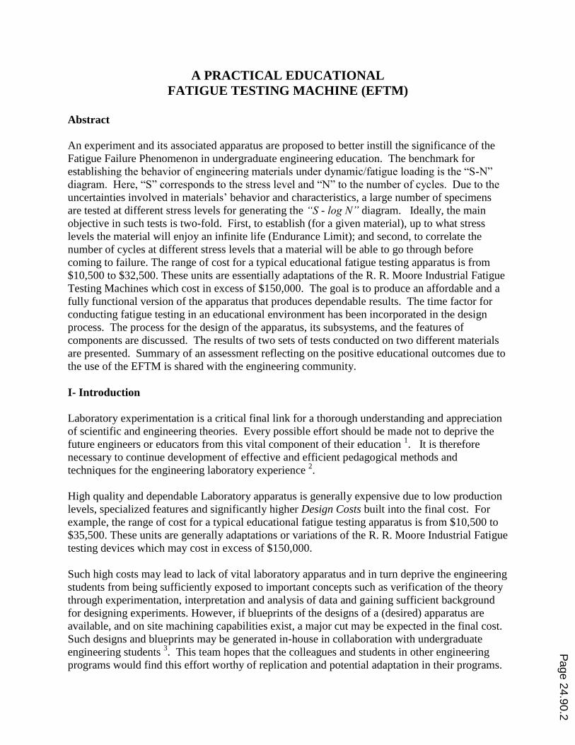
The benchmark for establishing the behavior of engineering materials under dynamic/fatigue

loading is the “S-N” diagram. Here, “S” corresponds to the stress level and “N” to the number of

cycles. Due to the uncertainties involved in the materials’ behavior and characteristics, a large

number of specimens are tested at different stress levels for generating the “S - log N” diagram.

Ideally, the main objective in such tests is two-fold. First, to establish (for a given material),

up to what stress levels the material will enjoy an infinite life (Endurance Limit); and second, to

correlate the number of cycles at different stress levels that a material will be able to go through

before failure.

Figure 1. S-N Diagram for Typical Behavior of Steel and Aluminum Alloys

Page 24.90.3

The S-N diagrams for several engineering materials have been established as a result of

comprehensive and highly time consuming tests. Generally, the results are more reliable for

steel alloys as compared with aluminum alloys. Low-cycle fatigue is defined on an S-N diagram

as being approximately between zero and 1000 cycles. High-cycle fatigue is generally greater

than 103 cycles. Finite life is assumed to be below 10

7 cycles

5. A typical S-N diagram is

shown in Figure (1).

Ferrous materials usually show a definite breaking point on the S-N diagram around 106 cycles,

whereas nonferrous metals show no such point. As shown in Figure (1), for nonferrous metals, a

value of 5x108 cycles is usually assigned as the fatigue limit. There are several theories available

for prediction of failure due to cyclic loading 6. Depending on the situation at hand, the designer

must apply the suitable theory as no one theory may optimally address all of the design

requirements. However, all of them converge on the fact that this type of failure is not yet

completely understood and extra care must be taken when dealing with fatigue phenomenon.

Shigley and Mischke present a rather comprehensive view of the issues involved with the

variations of behavior of different materials in the fatigue analysis process 7. The goal in the

current experiment is to create and simulate the conditions that allow students to test the

reliability of such (S-N) diagrams and gain a better understanding of the statistical and

probabilistic nature of the Fatigue Failure Theories.

III– Design of the Experiment and its Associated Apparatus

The following criteria have been incorporated in the design of the experiment and the associated

apparatus:

Safety

Simplicity and Practicality in Fabrication (at other institutions)

Affordability/Control of Cost

Use of Reliable Sources for Components

Durability

Use of Non-Corrosive & Aesthetically Pleasing Materials

Simplicity of Operation

NO use of Discontinued Parts/Components

Time Factor in Conducting the Experiment

The requirement of having a modular design and stopping the motor (when the specimen fails)

presented some interesting challenges. Additionally, the size, weight, and other physical

characteristics of the experiment were not defined at the inception of the project. Initially, this

lack of constraints may have been a blessing (for the students) since it did free the design process

to vary these factors. However, later, it became clear that the price for such a freedom is dealing

with the lack of starting points/values in the process. Table (1) provides a synopsis of the steps

and the parameters involved in the implementation of the project.

Page 24.90.4

Table 1. Steps and the Parameters involved in the successful implementation of the project.

#

TYPE OF ACTIVITY

1 Brainstorming for Design of the Experiment and the Apparatus

2 Meeting Minutes and Progress Reports

3 Prototyping

4 Generation of Technical Drawings for all (Home Made) Components

5 Selection of (commercial) Components and Identification of Suitable Sources

6 Fabrication and Compilation of Notes on Best Approach for Machining

7 Electro-mechanical control system

8 Testing, Calibration, Generation of Data and Measure of Precision and Accuracy

9 Generation of the Laboratory Manual for the Experiment

10 Loading of All Necessary Information and Helpful Links on a CD

IV- Theories of Fatigue Failure

To better appreciate the complexity of the fatigue phenomenon, Theories of Fatigue Failure

were comprehensively reviewed (by the collaborating students). These were further examined

and used as a visual platform to decide on the degree of sensitivity of the apparatus. Further,

they serve as indicators by which a laboratory coordinator/instructor may make more informed

decisions about the time required for conducting the experiment/ demonstration. A summary of

these models are presented in Appendix (A) 8.

V- Design of the Components and the Subsystems of the Apparatus

A simple schematic of the proposed Educational Fatigue Testing Machine (EFTM) is shown in

Figure (2). The first completed (full scale) prototype of the EFTM is shown in Figure (3).

We note that [as compared with the schematic shown in Figure (2),] the final design of the

apparatus eliminates the need for use of gears for reduction/control of the RPM. This was

achieved by employing a motor with the desired RPM (of 1725) allowing for a Direct-Drive

system.

EFTM is comprised of the following major components and subsystems. The role and design

characteristics of each of these components are briefly discussed.

1. The Base

In order to construct the apparatus, a suitable base needed to be acquired. A 0.5 inch thick by

6.75”x23” plate of 6061-T6 anodized aluminum proved to be strong enough to provide room for

installation of all of the components.

Page 24.90.5

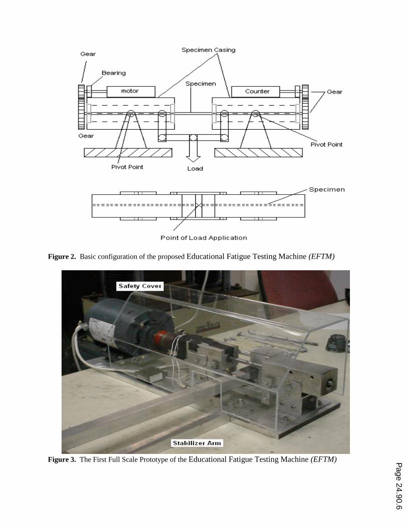
Figure 2. Basic configuration of the proposed Educational Fatigue Testing Machine (EFTM)

Figure 3. The First Full Scale Prototype of the Educational Fatigue Testing Machine (EFTM)

Page 24.90.6

2. The Motor

The choice of the most reliable and safe motor was critical. The research led to the selection of

an AC powered ¼ hp motor that included thermal protection and bearings.

3. The Gears and the Drive System

The importance of the gear system is much more than simply to rotate the specimen. The gears

also function as clamps to secure the specimen from translating inside the specimen holders

during testing. Since the specimen needs to be easily removed and replaced, the selection of the

clamping style of the gears, and the way that they mesh is important. However, in the current

design, the selection of the motor enabled the team to take advantage of a “direct drive” system

resulting in the elimination of a good number of components and significant reduction in cost.

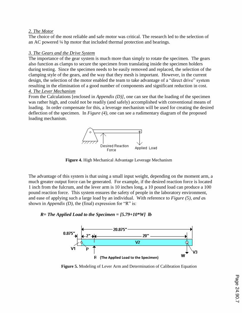
4. The Lever Mechanism

From the Calculations [enclosed in Appendix (D)], one can see that the loading of the specimen

was rather high, and could not be readily (and safely) accomplished with conventional means of

loading. In order compensate for this, a leverage mechanism will be used for creating the desired

deflection of the specimen. In Figure (4), one can see a rudimentary diagram of the proposed

loading mechanism.

Figure 4. High Mechanical Advantage Leverage Mechanism

The advantage of this system is that using a small input weight, depending on the moment arm, a

much greater output force can be generated. For example, if the desired reaction force is located

1 inch from the fulcrum, and the lever arm is 10 inches long, a 10 pound load can produce a 100

pound reaction force. This system ensures the safety of people in the laboratory environment,

and ease of applying such a large load by an individual. With reference to Figure (5), and as

shown in Appendix (D), the (final) expression for “R” is:

R= The Applied Load to the Specimen = [5.79+10*W] lb

Figure 5. Modeling of Lever Arm and Determination of Calibration Equation

(The Applied Load to the Specimen)

Page 24.90.7

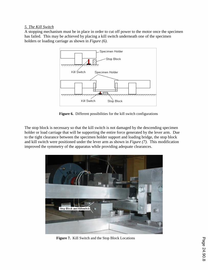
5. The Kill Switch

A stopping mechanism must be in place in order to cut off power to the motor once the specimen

has failed. This may be achieved by placing a kill switch underneath one of the specimen

holders or loading carriage as shown in Figure (6).

Figure 6. Different possibilities for the kill switch configurations

The stop block is necessary so that the kill switch is not damaged by the descending specimen

holder or load carriage that will be supporting the entire force generated by the lever arm. Due

to the tight clearance between the specimen holder support and loading bridge, the stop block

and kill switch were positioned under the lever arm as shown in Figure (7). This modification

improved the symmetry of the apparatus while providing adequate clearances.

Figure 7. Kill Switch and the Stop Block Locations

Page 24.90.8

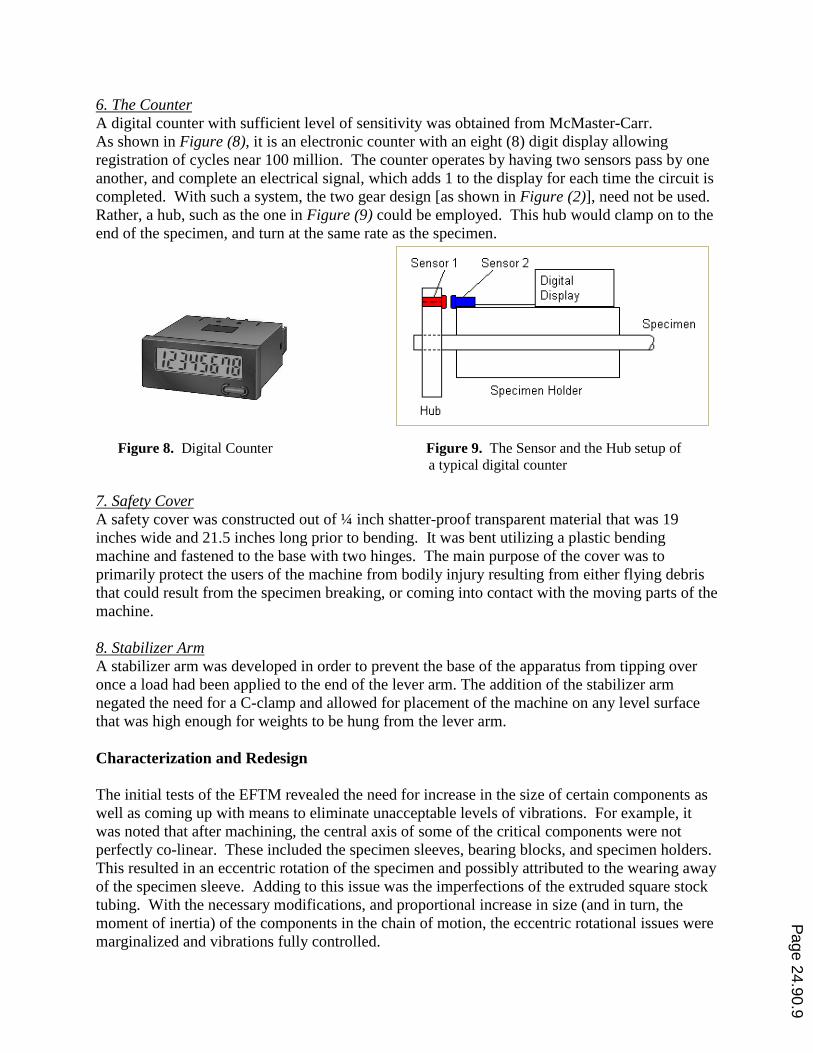
6. The Counter

A digital counter with sufficient level of sensitivity was obtained from McMaster-Carr.

As shown in Figure (8), it is an electronic counter with an eight (8) digit display allowing

registration of cycles near 100 million. The counter operates by having two sensors pass by one

another, and complete an electrical signal, which adds 1 to the display for each time the circuit is

completed. With such a system, the two gear design [as shown in Figure (2)], need not be used.

Rather, a hub, such as the one in Figure (9) could be employed. This hub would clamp on to the

end of the specimen, and turn at the same rate as the specimen.

Figure 8. Digital Counter Figure 9. The Sensor and the Hub setup of

a typical digital counter

7. Safety Cover

A safety cover was constructed out of ¼ inch shatter-proof transparent material that was 19

inches wide and 21.5 inches long prior to bending. It was bent utilizing a plastic bending

machine and fastened to the base with two hinges. The main purpose of the cover was to

primarily protect the users of the machine from bodily injury resulting from either flying debris

that could result from the specimen breaking, or coming into contact with the moving parts of the

machine.

8. Stabilizer Arm

A stabilizer arm was developed in order to prevent the base of the apparatus from tipping over

once a load had been applied to the end of the lever arm. The addition of the stabilizer arm

negated the need for a C-clamp and allowed for placement of the machine on any level surface

that was high enough for weights to be hung from the lever arm.

Characterization and Redesign

The initial tests of the EFTM revealed the need for increase in the size of certain components as

well as coming up with means to eliminate unacceptable levels of vibrations. For example, it

was noted that after machining, the central axis of some of the critical components were not

perfectly co-linear. These included the specimen sleeves, bearing blocks, and specimen holders.

This resulted in an eccentric rotation of the specimen and possibly attributed to the wearing away

of the specimen sleeve. Adding to this issue was the imperfections of the extruded square stock

tubing. With the necessary modifications, and proportional increase in size (and in turn, the

moment of inertia) of the components in the chain of motion, the eccentric rotational issues were

marginalized and vibrations fully controlled.

Page 24.90.9

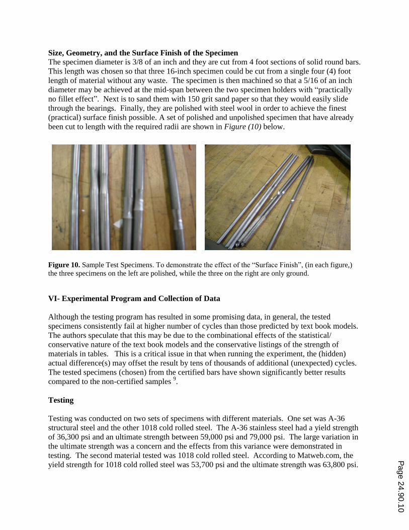
Size, Geometry, and the Surface Finish of the Specimen

The specimen diameter is 3/8 of an inch and they are cut from 4 foot sections of solid round bars.

This length was chosen so that three 16-inch specimen could be cut from a single four (4) foot

length of material without any waste. The specimen is then machined so that a 5/16 of an inch

diameter may be achieved at the mid-span between the two specimen holders with “practically

no fillet effect”. Next is to sand them with 150 grit sand paper so that they would easily slide

through the bearings. Finally, they are polished with steel wool in order to achieve the finest

(practical) surface finish possible. A set of polished and unpolished specimen that have already

been cut to length with the required radii are shown in Figure (10) below.

Figure 10. Sample Test Specimens. To demonstrate the effect of the “Surface Finish”, (in each figure,)

the three specimens on the left are polished, while the three on the right are only ground.

VI- Experimental Program and Collection of Data

Although the testing program has resulted in some promising data, in general, the tested

specimens consistently fail at higher number of cycles than those predicted by text book models.

The authors speculate that this may be due to the combinational effects of the statistical/

conservative nature of the text book models and the conservative listings of the strength of

materials in tables. This is a critical issue in that when running the experiment, the (hidden)

actual difference(s) may offset the result by tens of thousands of additional (unexpected) cycles.

The tested specimens (chosen) from the certified bars have shown significantly better results

compared to the non-certified samples 9.

Testing

Testing was conducted on two sets of specimens with different materials. One set was A-36

structural steel and the other 1018 cold rolled steel. The A-36 stainless steel had a yield strength

of 36,300 psi and an ultimate strength between 59,000 psi and 79,000 psi. The large variation in

the ultimate strength was a concern and the effects from this variance were demonstrated in

testing. The second material tested was 1018 cold rolled steel. According to Matweb.com, the

yield strength for 1018 cold rolled steel was 53,700 psi and the ultimate strength was 63,800 psi.

Page 24.90.10

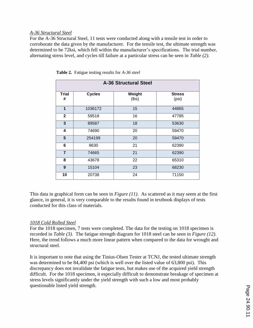
A-36 Structural Steel

For the A-36 Structural Steel, 11 tests were conducted along with a tensile test in order to

corroborate the data given by the manufacturer. For the tensile test, the ultimate strength was

determined to be 72ksi, which fell within the manufacturer’s specifications. The trial number,

alternating stress level, and cycles till failure at a particular stress can be seen in Table (2).

Table 2. Fatigue testing results for A-36 steel

A-36 Structural Steel

Trial #

Cycles

Weight (lbs)

Stress (psi)

1 1036172 15 44865

2 59518 16 47785

3 89587 18 53630

4 74690 20 59470

5 254199 20 59470

6 9630 21 62390

7 74665 21 62390

8 43678 22 65310

9 15104 23 68230

10 20738 24 71150

This data in graphical form can be seen in Figure (11). As scattered as it may seem at the first

glance, in general, it is very comparable to the results found in textbook displays of tests

conducted for this class of materials.

1018 Cold Rolled Steel

For the 1018 specimen, 7 tests were completed. The data for the testing on 1018 specimen is

recorded in Table (3). The fatigue strength diagram for 1018 steel can be seen in Figure (12).

Here, the trend follows a much more linear pattern when compared to the data for wrought and

structural steel.

It is important to note that using the Tinius-Olsen Tester at TCNJ, the tested ultimate strength

was determined to be 84,400 psi (which is well over the listed value of 63,800 psi). This

discrepancy does not invalidate the fatigue tests, but makes use of the acquired yield strength

difficult. For the 1018 specimen, it especially difficult to demonstrate breakage of specimen at

stress levels significantly under the yield strength with such a low and most probably

questionable listed yield strength. Page 24.90.11

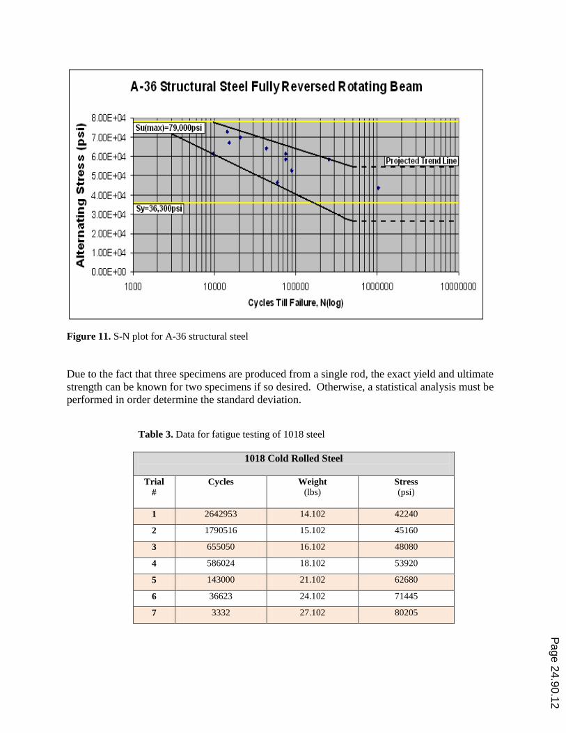
Figure 11. S-N plot for A-36 structural steel

Due to the fact that three specimens are produced from a single rod, the exact yield and ultimate

strength can be known for two specimens if so desired. Otherwise, a statistical analysis must be

performed in order determine the standard deviation.

Table 3. Data for fatigue testing of 1018 steel

1018 Cold Rolled Steel

Trial

#

Cycles

Weight

(lbs)

Stress

(psi)

1 2642953 14.102 42240

2 1790516 15.102 45160

3 655050 16.102 48080

4 586024 18.102 53920

5 143000 21.102 62680

6 36623 24.102 71445

7 3332 27.102 80205

Page 24.90.12

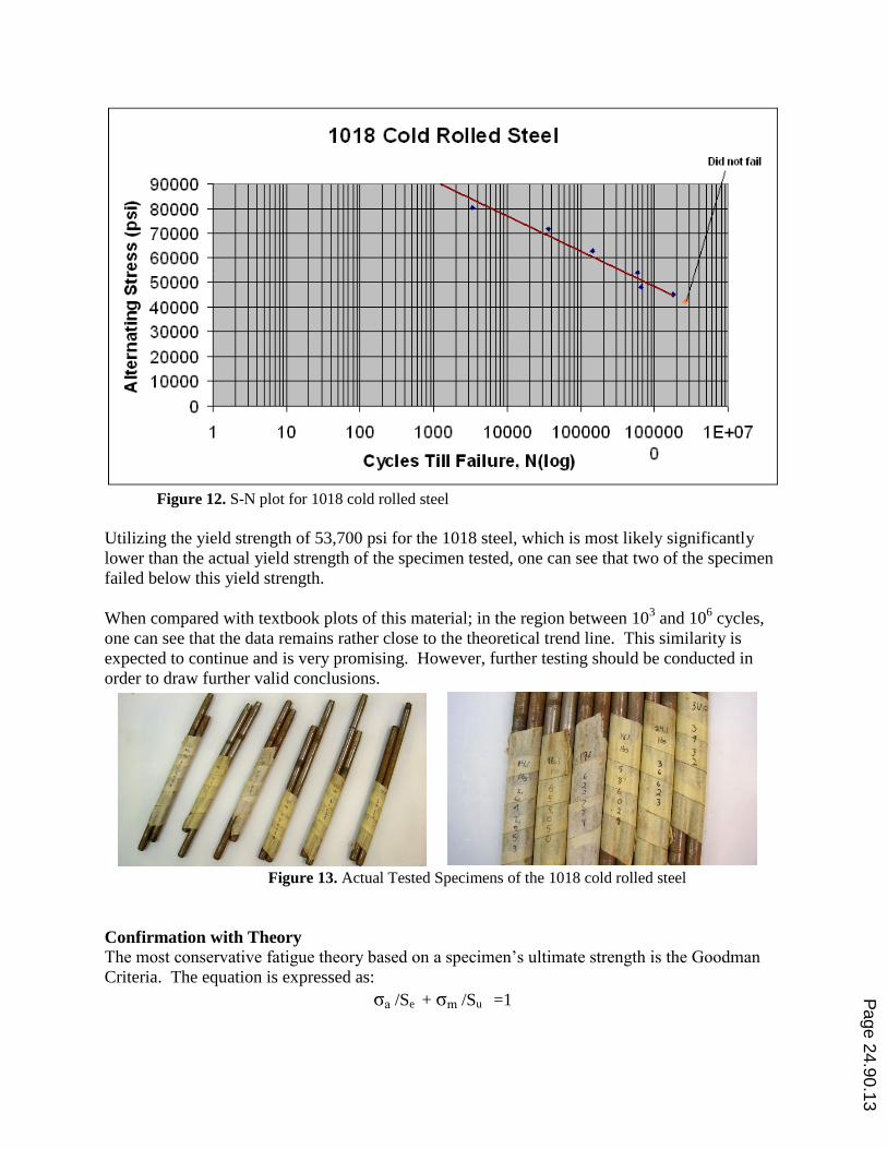
Figure 12. S-N plot for 1018 cold rolled steel

Utilizing the yield strength of 53,700 psi for the 1018 steel, which is most likely significantly

lower than the actual yield strength of the specimen tested, one can see that two of the specimen

failed below this yield strength.

When compared with textbook plots of this material; in the region between 103 and 10

6 cycles,

one can see that the data remains rather close to the theoretical trend line. This similarity is

expected to continue and is very promising. However, further testing should be conducted in

order to draw further valid conclusions.

Figure 13. Actual Tested Specimens of the 1018 cold rolled steel

Confirmation with Theory The most conservative fatigue theory based on a specimen’s ultimate strength is the Goodman

Criteria. The equation is expressed as:

σa /Se + σm /Su =1

Page 24.90.13

Where Se is the endurance strength, Su is the ultimate strength, and σa and σm are the alternating

and average stress, respectively. The average stress is zero due to nature of rotating beam fatigue

testing, and the equation simplifies to:

σa/ Se = 1

Taking an approximate endurance stress/strength of 42,200 psi for 1018 cold rolled steel, which

is the stress level for the specimen that has yet to fail, any stress level above 42,200 psi will

result in a value larger than 1 for σa/ Se. This means that any alternating stress level above

42,200 psi will result in failure of the 1018 specimen. This is exactly what can be seen for every

value test for the 1018 specimen.

VII– Observations

The following is a listing of the interesting observations made up to this point in the process:

1. All solid specimens with reduced diameter (at center) failed at the Mid-Span,

2. All specimens with discontinuities (near the Mid-Span) failed at the discontinuity,

3. All specimens failed at higher (more conservative) values than expected/listed,

4. Certified specimens fail at values closer to the predicted ones than the non-certified ones,

5. Steel specimens fail at values closer to the predicted ones than the Aluminum samples,

6. Failure of all specimens was abrupt-no warning,

7. The test results may be considered as Precise but certainly not perfectly Accurate.

VIII– Recommendations

The following recommendations may be made at this stage of the task:

1. Avoid the use of small diameter sections as the variation in results may become quite

troublesome-[do not use sections with a (effective) diameter of less than 1/8” for Steel

and less than 1/4” for Aluminum],

2. Work with specimens that have a Length to Diameter Ratio of: 12 L / DEffective 25,

3. In reduction of the diameter of the specimen in the mid-span; to avoid Stress

Concentration, do not use “fillets”(even with maximum possible radius),

4. Select motors that provide a reasonable combination of power and RPM,

5. If you choose to work with aluminum, don’t set it as the base metal for the experiment,

6. Try to obtain materials with certification as this may save you a great deal of time,

7. If possible, run a complete tensile test on a sample of the bars used for the specimens,

8. If possible, cut “all” of the specimen (in one set of tests) from the “same” bar,

9. To examine potential variations (perhaps due to set-up), double/triple the number of tests

for a “single” level of stress,

10. Exercise the safety precautions in this experiment to the full extent,

11. Obtain the most updated results and recommended procedures from the authors,

12. Share your findings and Alternative Solutions with the authors so that they may share

them with other interested parties.

Page 24.90.14

IX – Total Cost of EFTM

A complete list of the materials and the components for construction of the proposed EFTM is

presented in Appendix (E). In addition, we have taken extra care in recording the machining and

assembly times for the creation of the apparatus. The total (conservatively) estimated cost of

$2,500 is certainly an attractive figure. It goes without saying that several hundreds of hours

have been dedicated by the collaborating students in the design and fabrication of the tester.

X – A Short Assessment

The authors used the audience in two of the sections of the Mechanical Design and Analysis

course at TCNJ for their short assessment. The object for this exercise was to measure if the

observations and the running of the tests on the 1018 CR Steel specimens made a noticeable

difference in the better understanding of the fatigue phenomenon. A Laboratory handout has

been created for running the experiment. Please see Appendix (F).

Ordinarily, a Rating and Assessment form is handed out for this type of activity at TCNJ. This

form is included in Appendix (G). Tables (H-1) through ( H-3) [placed in Appendix (H)] provide

detailed summaries of the results for three of the (more measurable) questions on the project’s

assessment form.

Nearly all participants state that they would incorporate an activity of this nature should they get

the opportunity to teach a similar course. The assessment results clearly reflect on the fact that

there is (nearly perfect) consensus that the project is a balanced activity that is highly valued by

the members of the fifteen (15) groups. They also shared their thoughts on how their exposure to

the testing process and completion of the exercise has influenced their much better understanding

and appreciation of these important criteria in “failure prevention”.

XI – Summary and Conclusions

An affordable and a fully functional educational version of the R. R. Moore Fatigue Testing

apparatus that produces dependable results is proposed for national adaptation. Junior and senior

Engineering students have collaborated in the design and fabrication of the apparatus. The time

factor for conducting fatigue testing in an educational environment has been incorporated in the

design process. The process for the design of the apparatus, its subsystems, and the features of

components are disclosed in details. A complete list of the materials and the components for

construction of the proposed Educational Fatigue Testing Machine (EFTM) is provided. Full

details of two sets of tests conducted on two different materials are presented. A sample

Laboratory Handout is enclosed for examining the potential of the unit for conducting

meaningful experiments. Summary of a short/preliminary assessment reflecting on the positive

educational outcomes due to the use of this apparatus is shared with the engineering community.

It is believed that in comparison with the commercially available counterparts of the EFTM, an

alternative solution is offered that may prove feasible for implementation. This approach is

beneficial for all parties involved including; the researching/collaborating student(s),

underclassmen who would benefit from such experiments, and the enthusiastic instructors/

Page 24.90.15

laboratory coordinators who may be fighting with budgetary issues. The only remaining obstacle

is the better understanding of why the experimentally obtained number of cycles are

conservatively higher than the (theoretically) predicted ones. So, further examination of the text

book models/equations and search for ascertaining materials that do not suffer from a large

standard deviation (from the expected mean) should continue. However, although we have not

yet achieved an impressive level of “accuracy”, we can clearly conclude that the results are

certainly “precise”.

Acknowledgements

The authors express special thanks to Alexander Michalchuk (former department senior

technician and machinist) and Joseph Zanetti (current Machine Shop Supervisor) for their

continuous support and dedication to the project.

References

1. Sepahpour, B., “Design of an Affordable Model Laboratory for Mechanical and Civil Engineering

Programs”, Proceedings of ASEE 2003 National Conference, Nashville, TN, June 2003.

2. Sepahpour, B., Clark, E. and Limberis, L. “Modular Lumped Mass Experiment”, Proceedings of

ASEE 2004 National Conference, Salt Lake City, Utah, June 2004.

3. Sepahpour, B., “Involving Undergraduate Students in Design of Experiments”, Proceedings of ASEE

2002 National Conference, Montreal, Canada, June 2002.

4. Young, W. C. and Budynas G. Roark’s Formulas for Stress and Strain, Seventh Edition.

McGraw Hill, 2002.

5. Ugural, Ansel C. Mechanical Design: An Integrated Approach. International Edition. McGraw Hill

Higher Education, 2004.

6. Juvinal, R. C., and Marshek, K. M. Fundamentals of Machine Component Design. Third Edition.

John Wiley & Sons, 2000.

7. Shigley, J. E. and Mischke, C. R. Standard Handbook of Machine Design. McGraw Hill, 1986.

8. Shigley, Joseph E. Mechanical Engineering Design, Third Edition, McGraw Hill, 1980.

9. Sepahpour, B., and Chang, S.R. “Low Cycle and Finite Life Fatigue Experiment”, Proceedings of

ASEE 2005 National Conference, Portland, OR, June 2005, June 2005.

Page 24.90.16

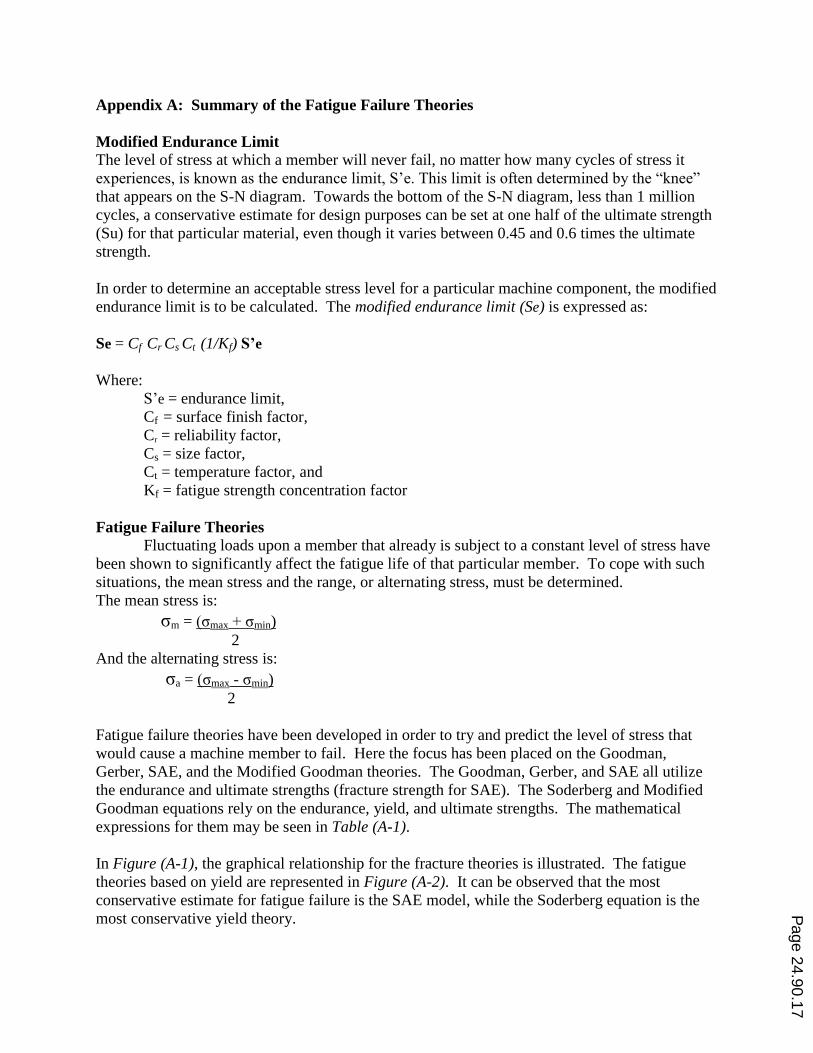
Appendix A: Summary of the Fatigue Failure Theories

Modified Endurance Limit

The level of stress at which a member will never fail, no matter how many cycles of stress it

experiences, is known as the endurance limit, S’e. This limit is often determined by the “knee”

that appears on the S-N diagram. Towards the bottom of the S-N diagram, less than 1 million

cycles, a conservative estimate for design purposes can be set at one half of the ultimate strength

(Su) for that particular material, even though it varies between 0.45 and 0.6 times the ultimate

strength.

In order to determine an acceptable stress level for a particular machine component, the modified

endurance limit is to be calculated. The modified endurance limit (Se) is expressed as:

Se = Cf Cr Cs Ct (1/Kf) S’e

Where:

S’e = endurance limit,

Cf = surface finish factor,

Cr = reliability factor,

Cs = size factor,

Ct = temperature factor, and

Kf = fatigue strength concentration factor

Fatigue Failure Theories

Fluctuating loads upon a member that already is subject to a constant level of stress have

been shown to significantly affect the fatigue life of that particular member. To cope with such

situations, the mean stress and the range, or alternating stress, must be determined.

The mean stress is:

σm = (σmax + σmin)

2

And the alternating stress is:

σa = (σmax - σmin)

2

Fatigue failure theories have been developed in order to try and predict the level of stress that

would cause a machine member to fail. Here the focus has been placed on the Goodman,

Gerber, SAE, and the Modified Goodman theories. The Goodman, Gerber, and SAE all utilize

the endurance and ultimate strengths (fracture strength for SAE). The Soderberg and Modified

Goodman equations rely on the endurance, yield, and ultimate strengths. The mathematical

expressions for them may be seen in Table (A-1).

In Figure (A-1), the graphical relationship for the fracture theories is illustrated. The fatigue

theories based on yield are represented in Figure (A-2). It can be observed that the most

conservative estimate for fatigue failure is the SAE model, while the Soderberg equation is the

most conservative yield theory.

Page 24.90.17

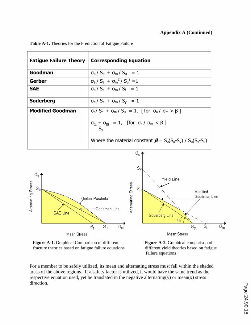
Appendix A (Continued) Table A-1. Theories for the Prediction of Fatigue Failure

Fatigue Failure Theory

Corresponding Equation

Goodman σa / Se + σm / Su = 1

Gerber σa / Se + σm2 / Su

2 =1

SAE σa / Se + σm / Sf = 1

Soderberg σa / Se + σm / Sy = 1

Modified Goodman σa/ Se + σm / Su = 1, [ for σa / σm > β ]

σa + σm = 1, [for σa / σm < β ]

Sy

Where the material constant β = Se(Su-Sy) / Su(Sy-Se)

Figure A-1. Graphical Comparison of different Figure A-2. Graphical comparison of

fracture theories based on fatigue failure equations different yield theories based on fatigue

failure equations

For a member to be safely utilized, its mean and alternating stress must fall within the shaded

areas of the above regions. If a safety factor is utilized, it would have the same trend as the

respective equation used, yet be translated in the negative alternating(y) or mean(x) stress

direction.

Yield Line

Page 24.90.18

Appendix B: Summary of the Stress calculations

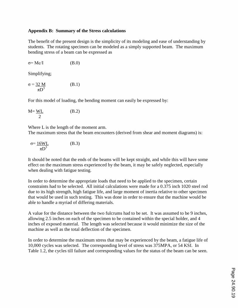
The benefit of the present design is the simplicity of its modeling and ease of understanding by

students. The rotating specimen can be modeled as a simply supported beam. The maximum

bending stress of a beam can be expressed as

σ= Mc/I (B.0)

Simplifying;

σ = 32 M (B.1)

πD3

For this model of loading, the bending moment can easily be expressed by:

M= WL (B.2)

2

Where L is the length of the moment arm.

The maximum stress that the beam encounters (derived from shear and moment diagrams) is:

σ= 16WL (B.3)

πD3

It should be noted that the ends of the beams will be kept straight, and while this will have some

effect on the maximum stress experienced by the beam, it may be safely neglected, especially

when dealing with fatigue testing.

In order to determine the appropriate loads that need to be applied to the specimen, certain

constraints had to be selected. All initial calculations were made for a 0.375 inch 1020 steel rod

due to its high strength, high fatigue life, and large moment of inertia relative to other specimen

that would be used in such testing. This was done in order to ensure that the machine would be

able to handle a myriad of differing materials.

A value for the distance between the two fulcrums had to be set. It was assumed to be 9 inches,

allowing 2.5 inches on each of the specimen to be contained within the special holder, and 4

inches of exposed material. The length was selected because it would minimize the size of the

machine as well as the total deflection of the specimen.

In order to determine the maximum stress that may be experienced by the beam, a fatigue life of

10,000 cycles was selected. The corresponding level of stress was 375MPA, or 54 KSI. In

Table 1.2, the cycles till failure and corresponding values for the status of the beam can be seen.

Page 24.90.19

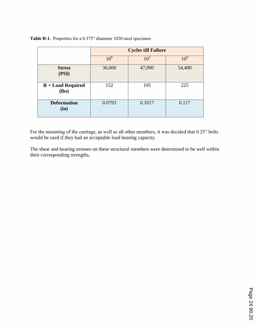
Table B-1. Properties for a 0.375” diameter 1020 steel specimen

Cycles till Failure

106 10

5 10

4

Stress

(PSI)

36,600 47,000 54,400

R = Load Required

(lbs)

152 195 225

Deformation

(in)

0.0793 0.1017 0.117

For the mounting of the carriage, as well as all other members, it was decided that 0.25” bolts

would be used if they had an acceptable load bearing capacity.

The shear and bearing stresses on these structural members were determined to be well within

their corresponding strengths.

Page 24.90.20

Appendix C: Critical Speed of the Shaft

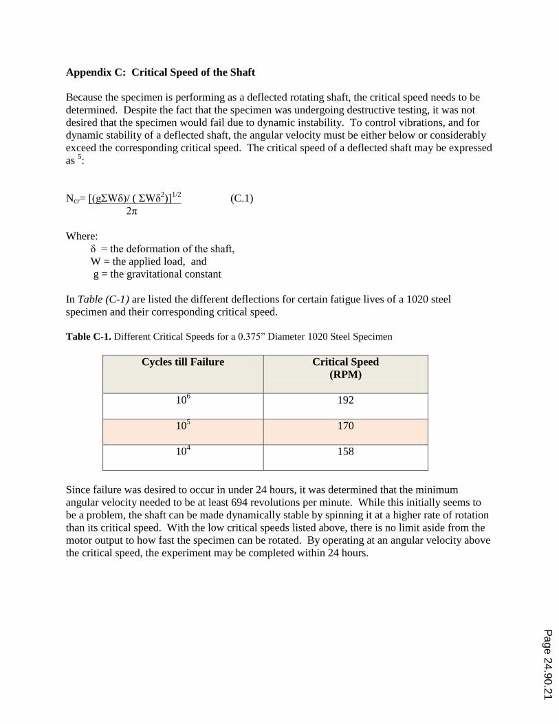
Because the specimen is performing as a deflected rotating shaft, the critical speed needs to be

determined. Despite the fact that the specimen was undergoing destructive testing, it was not

desired that the specimen would fail due to dynamic instability. To control vibrations, and for

dynamic stability of a deflected shaft, the angular velocity must be either below or considerably

exceed the corresponding critical speed. The critical speed of a deflected shaft may be expressed

as 5:

Ncr= [(gΣWδ)/ ( ΣWδ2)]

1/2 (C.1)

2π

Where:

δ = the deformation of the shaft,

W = the applied load, and

g = the gravitational constant

In Table (C-1) are listed the different deflections for certain fatigue lives of a 1020 steel

specimen and their corresponding critical speed.

Table C-1. Different Critical Speeds for a 0.375” Diameter 1020 Steel Specimen

Cycles till Failure Critical Speed

(RPM)

106 192

105 170

104 158

Since failure was desired to occur in under 24 hours, it was determined that the minimum

angular velocity needed to be at least 694 revolutions per minute. While this initially seems to

be a problem, the shaft can be made dynamically stable by spinning it at a higher rate of rotation

than its critical speed. With the low critical speeds listed above, there is no limit aside from the

motor output to how fast the specimen can be rotated. By operating at an angular velocity above

the critical speed, the experiment may be completed within 24 hours.

Page 24.90.21

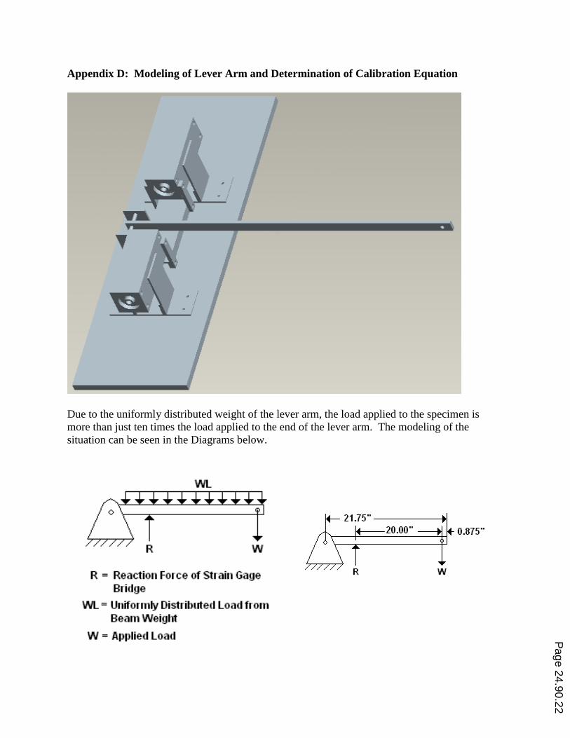
Appendix D: Modeling of Lever Arm and Determination of Calibration Equation

Due to the uniformly distributed weight of the lever arm, the load applied to the specimen is

more than just ten times the load applied to the end of the lever arm. The modeling of the

situation can be seen in the Diagrams below.

Page 24.90.22

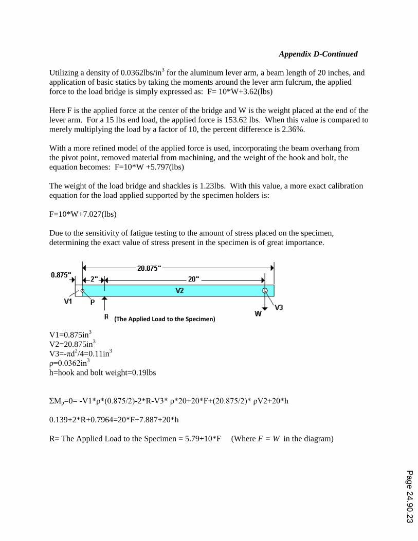
Appendix D-Continued

Utilizing a density of 0.0362lbs/in3 for the aluminum lever arm, a beam length of 20 inches, and

application of basic statics by taking the moments around the lever arm fulcrum, the applied

force to the load bridge is simply expressed as: F= 10*W+3.62(lbs)

Here F is the applied force at the center of the bridge and W is the weight placed at the end of the

lever arm. For a 15 lbs end load, the applied force is 153.62 lbs. When this value is compared to

merely multiplying the load by a factor of 10, the percent difference is 2.36%.

With a more refined model of the applied force is used, incorporating the beam overhang from

the pivot point, removed material from machining, and the weight of the hook and bolt, the

equation becomes: F=10*W +5.797(lbs)

The weight of the load bridge and shackles is 1.23lbs. With this value, a more exact calibration

equation for the load applied supported by the specimen holders is:

F=10*W+7.027(lbs)

Due to the sensitivity of fatigue testing to the amount of stress placed on the specimen,

determining the exact value of stress present in the specimen is of great importance.

V1=0.875in3

V2=20.875in3

V3=-πd2/4=0.11in

3

ρ=0.0362in3

h=hook and bolt weight=0.19lbs

ΣMp=0= -V1*ρ*(0.875/2)-2*R-V3* ρ*20+20*F+(20.875/2)* ρV2+20*h

0.139+2*R+0.7964=20*F+7.887+20*h

R= The Applied Load to the Specimen = 5.79+10*F (Where F = W in the diagram)

(The Applied Load to the Specimen)

Page 24.90.23

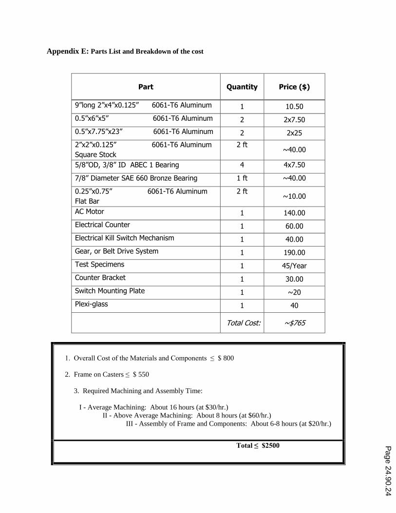
Appendix E: Parts List and Breakdown of the cost

Part Quantity

Price ($)

9”long 2”x4”x0.125” 6061-T6 Aluminum 1 10.50

0.5”x6”x5” 6061-T6 Aluminum 2 2x7.50

0.5”x7.75”x23” 6061-T6 Aluminum 2 2x25

2”x2”x0.125” 6061-T6 Aluminum

Square Stock

2 ft ~40.00

5/8”OD, 3/8” ID ABEC 1 Bearing 4 4x7.50

7/8” Diameter SAE 660 Bronze Bearing 1 ft ~40.00

0.25”x0.75” 6061-T6 Aluminum

Flat Bar

2 ft ~10.00

AC Motor 1 140.00

Electrical Counter 1 60.00

Electrical Kill Switch Mechanism 1 40.00

Gear, or Belt Drive System 1 190.00

Test Specimens 1 45/Year

Counter Bracket 1 30.00

Switch Mounting Plate 1 ~20

Plexi-glass 1 40

Total Cost: ~$765

1. Overall Cost of the Materials and Components ≤ $ 800

2. Frame on Casters ≤ $ 550

3. Required Machining and Assembly Time:

I - Average Machining: About 16 hours (at $30/hr.)

II - Above Average Machining: About 8 hours (at $60/hr.)

III - Assembly of Frame and Components: About 6-8 hours (at $20/hr.)

Total ≤ $2500 Page 24.90.24

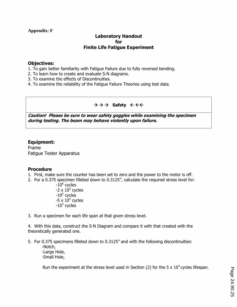
Appendix: F

Laboratory Handout for

Finite Life Fatigue Experiment

Objectives: 1. To gain better familiarity with Fatigue Failure due to fully reversed bending. 2. To learn how to create and evaluate S-N diagrams. 3. To examine the effects of Discontinuities. 4. To examine the reliability of the Fatigue Failure Theories using test data.

Safety

Caution! Please be sure to wear safety goggles while examining the specimen during testing. The beam may behave violently upon failure.

Equipment: Frame Fatigue Tester Apparatus

Procedure 1. First, make sure the counter has been set to zero and the power to the motor is off. 2. For a 0.375 specimen filleted down to 0.3125”, calculate the required stress level for: -106 cycles -2 x 105 cycles -105 cycles -5 x 104 cycles -104 cycles 3. Run a specimen for each life span at that given stress level. 4. With this data, construct the S-N Diagram and compare it with that created with the theoretically generated one. 5. For 0.375 specimens filleted down to 0.3125” and with the following discontinuities: -Notch, -Large Hole, -Small Hole, Run the experiment at the stress level used in Section (2) for the 5 x 104 cycles lifespan.

Page 24.90.25

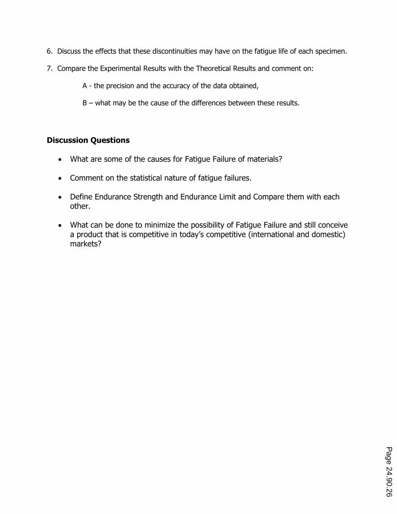
6. Discuss the effects that these discontinuities may have on the fatigue life of each specimen. 7. Compare the Experimental Results with the Theoretical Results and comment on: A - the precision and the accuracy of the data obtained, B – what may be the cause of the differences between these results.

Discussion Questions

What are some of the causes for Fatigue Failure of materials?

Comment on the statistical nature of fatigue failures.

Define Endurance Strength and Endurance Limit and Compare them with each other.

What can be done to minimize the possibility of Fatigue Failure and still conceive

a product that is competitive in today’s competitive (international and domestic) markets?

Page 24.90.26

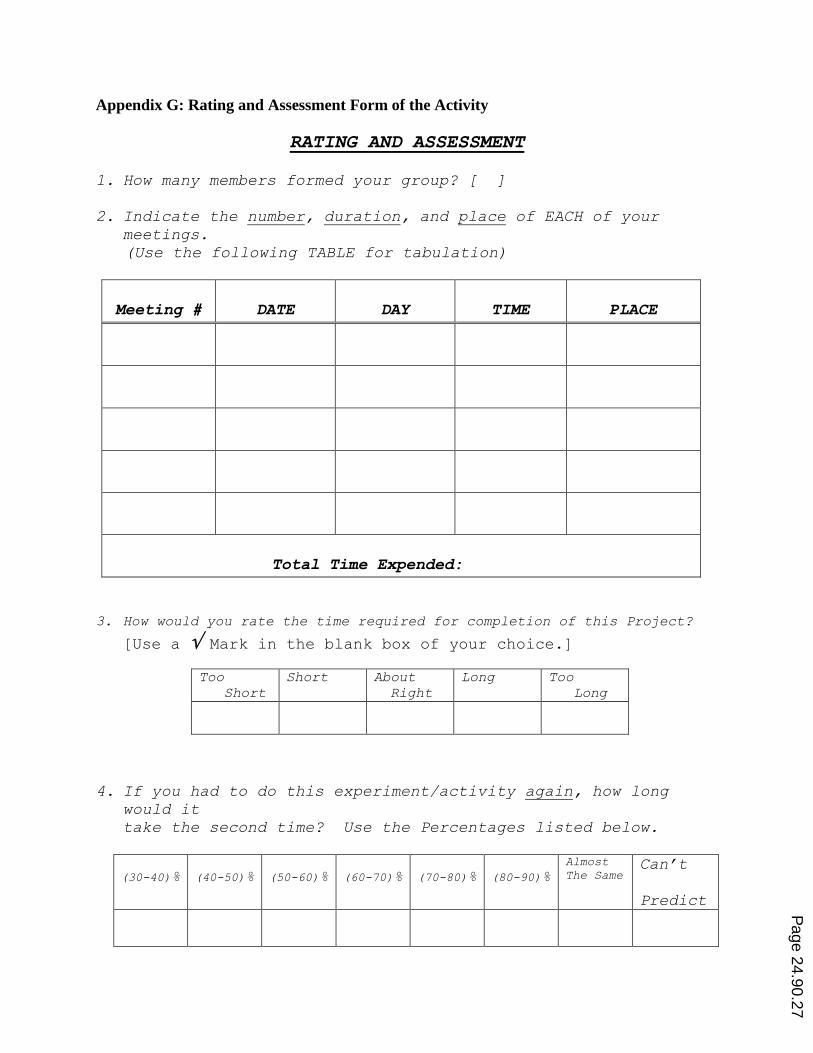
Appendix G: Rating and Assessment Form of the Activity

RATING AND ASSESSMENT

1. How many members formed your group? [ ]

2. Indicate the number, duration, and place of EACH of your meetings.

(Use the following TABLE for tabulation)

Meeting #

DATE

DAY

TIME

PLACE

Total Time Expended:

3. How would you rate the time required for completion of this Project?

[Use a Mark in the blank box of your choice.]

Too

Short

Short About

Right

Long Too

Long

4. If you had to do this experiment/activity again, how long would it

take the second time? Use the Percentages listed below.

(30-40)%

(40-50)%

(50-60)%

(60-70)%

(70-80)%

(80-90)% Almost

The Same Can’t

Predict

Page 24.90.27

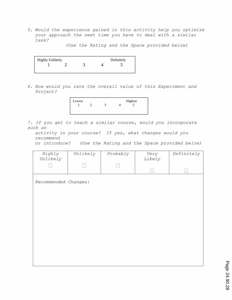
5. Would the experience gained in this activity help you optimize your approach the next time you have to deal with a similar

task?

(Use the Rating and the Space provided below)

6. How would you rate the overall value of this Experiment and Project?

7. If you get to teach a similar course, would you incorporate

such an

activity in your course? If yes, what changes would you

recommend

or introduce? (Use the Rating and the Space provided below)

Highly

Unlikely

Unlikely

Probably

Very

Likely

Definitely

Recommended Changes:

Lowest Highest

1 2 3 4 5

Highly Unlikely Definitely

1 2 3 4 5

Page 24.90.28

Appendix H: Tables for the Assessment

Table H-1. Summary of the Results for the First Measurable (and relevant) Question on the

Project Assessment Form

Question # 1: How would you rate the time required for completion of this Project?

xxxxxxxxxx Rating Section # # of Groups Too

Short

Short About

Right

Long Too

Long

01 7 - - 5 1 1

02 8 - - 6 2 -

Total N = 15 - - 11 3 1

Table H-2. Summary of the Results for the Second Measurable (and relevant) Question on the

Project Assessment Form

Question # 2: Would the experience gained in this activity help you optimize your approach the next time you have to deal with a similar task?

xxxxxxxxxx Rating Section # # of Groups Highly

Unlikely

Unlikely Probably Very

Likely

Definitely

01 7 - - - 4 3

02 8 - - 1 3 4

Total N = 15 - - 1 7 7

Table H-3. Summary of the Results for the Third Measurable (and relevant) Question on the

Project Assessment Form

Question # 3: How would you rate the overall Value of this Experiment and Project?

xxxxxxxxxx Rating

Section # # of Groups Very

Low

Low Medium High Very High

01 7 - - 1 4 2

02 8 - - - 6 2

Total N = 15 - - 1 10 4

Page 24.90.29