A practical grid-based method for tracking multiple ...rses.anu.edu.au/~malcolm/papers/pdf/dekool06.pdf · A practical grid-based method for tracking multiple refraction and reﬂection

$Page 1: A practical grid-based method for tracking multiple ...rses.anu.edu.au/~malcolm/papers/pdf/dekool06.pdf · A practical grid-based method for tracking multiple refraction and reﬂection$
Geophys. J. Int. (2006) 167, 253–270 doi: 10.1111/j.1365-246X.2006.03078.x

GJI

Sei

smol

ogy

A practical grid-based method for tracking multiple refractionand reflection phases in three-dimensional heterogeneous media

M. de Kool,∗ N. Rawlinson and M. SambridgeResearch School of Earth Sciences, Australian National University, Canberra, ACT 0200, Australia. E-mail: [email protected]

Accepted 2006 May 23. Received 2006 May 8; in original form 2005 August 21

S U M M A R YWe present a practical grid-based method in 3-D spherical coordinates for computing multiplephases comprising any number of reflection and transmission branches in heterogeneous lay-ered media. The new scheme is based on a multistage approach which treats each layer that thewave front enters as a separate computational domain. A finite-difference eikonal solver knownas the fast-marching method (FMM) is reinitialized at each interface to track the evolving wavefront as either a reflection back into the incident layer or a transmission through to the adjacentlayer. Unlike the standard FMM, which only finds first arrivals, this multistage approach cantrack those later arriving phases explicitly caused by the presence of discontinuities. Notably,the method does not require an irregular mesh to be constructed in order to connect interfacenodes to neighbouring velocity nodes which lie on a regular grid. To improve accuracy, localgrid refinement is used in the neighbourhood of a source point where wave front curvature ishigh. The method also provides a way to trace reflections from an interface that are not thefirst arrival (e.g. the global PP phase). These are computed by initializing the multistage FMMfrom both the source and receiver, propagating the two wave fronts to the reflecting interface,and finding stationary points of the sum of the two traveltime fields on the reflecting interface.

A series of examples are presented to test the efficiency, accuracy and robustness of thenew scheme. As well as efficiently computing various global phases to an acceptable accuracythrough the ak135 model, we also demonstrate the ability of the scheme to track complex crustalphases that may be encountered in coincident reflection, wide-angle reflection/refraction orlocal earthquake surveys. In one example, a variety of phases are computed in the presence ofa realistic subduction zone, which includes several layer pinch-outs and a subducting slab. Ournumerical tests show that the new scheme is a practical and robust alternative to conventionalray tracing for finding various phases in layered media at a variety of scales.

Key words: fast-marching method, finite-difference methods, ray tracing, seismic phases,seismic wave propagation, traveltime.

1 I N T RO D U C T I O N

Grid based (or ‘Eulerian’) traveltime prediction schemes are nowfirmly established as viable, if not preferable, alternatives to con-ventional ray-tracing (or ‘Lagrangian’) methods for computing firstarrival seismic traveltimes in the presence of heterogeneous 2-D or3-D media. One of the first practical grid-based schemes was devel-oped by Vidale (1988), who used finite-difference solutions of theeikonal equation to compute traveltimes throughout a gridded ve-locity field. Since this seminal paper, numerous schemes for solvingthe eikonal equation with finite differences have appeared (Podvin& Lecomte 1991; van Trier & Symes 1991; Qin et al. 1992; Cao

∗Now at: Geoscience Australia, Symonston ACT 2609, Australia.

& Greenhalgh 1994; Kim & Cook 1999; Afnimar & Koketsu 2000;Qian & Symes 2002).

An alternative grid-based scheme for computing seismic trav-eltimes, which is less widely used than finite-difference eikonalsolvers, is Shortest Path Raytracing or SPR. This approach appealsdirectly to Fermat’s principle of stationary time by using Dijkstra-like algorithms to locate minimum traveltime paths through a net-work or graph which connects the nodes of a gridded velocity field(Nakanishi & Yamaguchi 1986; Moser 1991; Fischer & Lees 1993;Cheng & House 1996). Finite-difference eikonal solvers and, toa lesser extent, SPR are now commonly used in several classes ofseismic imaging; for example, in refraction tomography (Hole 1992;Toomey et al. 1994; Zelt & Barton 1998; Day et al. 2001; Zelt et al.2001), and in the migration of coincident reflection sections (Gray& May 1994; Bevc 1997; Zhao et al. 1998; Buske 1999; Popovici& Sethian 2002).

C© 2006 The Authors 253Journal compilation C© 2006 RAS

254 M. de Kool, N. Rawlinson and M. Sambridge

Compared to conventional shooting and bending methods of ray-tracing (e.g. Julian & Gubbins 1977; Cassell 1982; Um & Thurber1987; Sambridge 1990; Koketsu & Sekine 1998) grid-based trav-eltime solvers have several distinct advantages. First, most are ca-pable of computing traveltimes to all points of a velocity medium,and will correctly find diffractions in ray shadow zones (Vidale1988). Secondly, while shooting and bending schemes may fail toconverge to the true two point path, even in mildly heterogeneousmedia, many grid-based schemes are highly stable and will con-verge to the correct solution. Thirdly, grid-based schemes can bevery efficient in computing traveltimes to the level of accuracy thatis required in practical problems, particularly when there is a largenumber of sources or receivers. Often due to the difficulty of lo-cating two point paths, ray tracing can be quite inefficient. Finally,finite-difference eikonal solvers and SPR are designed to consis-tently find the first-arrival traveltime in a continuous medium. Ray-tracing schemes also tend to only find single arrivals, but there is usu-ally no guarantee as to whether the selected arrival is a first or laterarrival.

First-arrival traveltimes are frequently used in seismic studies,but it is often the case that later arrivals carry most of the seismicenergy and hence dominate the recorded signal. One of the currentchallenges in seismic imaging is to exploit such arrivals in orderto produce more detailed and robust earth models. For this to hap-pen, efficient numerical schemes are required to predict all arrivalsof significant amplitude. The most practical and well developed ofsuch schemes to date is wave front construction (Vinje et al. 1993;Lambare et al. 1996; Vinje et al. 1999; Xu & Lambare 2004), whichpropagates a wave front in a series of time steps using local ray trac-ing and interpolation. However, complex data structures are requiredto keep track of the wave front, and parts of the wave front with highcurvature can be poorly resolved.

A number of grid-based schemes have been proposed for track-ing later arrivals. One approach is to partition the multivalued so-lution into a series of single-valued solutions and apply first-arrivalsolvers in each of the segregated regions (Benamou 1996; Symes& Qian 2003). Although computationally efficient, it is hard to seehow such a method can successfully locate all multipaths in complexmedia. Recently, several schemes based on the level set method havebeen proposed for tracking wave fronts in phase space (e.g. Fomel& Sethian 2002; Osher et al. 2002). While their potential for ro-bustly computing all arrivals has been demonstrated, further devel-opment is required, in particular to make them more computationallyefficient.

Although a practical Eulerian scheme for computing all multiplearrivals is yet to emerge, it should be possible to construct efficientand robust grid-based schemes to track a limited but useful classof later arriving phases associated with the presence of interfaces,which separate media of different wavespeed. So far, relatively fewstudies have attempted this, and ray tracing still appears to be themethod of choice in layered media, for example, when global phases(pP, PcP, PP etc.) or crustal reflections, refractions and multiples arerequired. One approach for computing reflections with a grid-basedtechnique is to track first-arrival traveltime fields from both sourceand receiver to the entire interface, and then use Fermat’s princi-ple of stationary time to locate reflection points along the interface(Podvin & Lecomte 1991; Riahi & Juhlin 1994). Using the 3-Dfinite-difference scheme of Vidale (1990), Hole & Zelt (1995) as-sumed that the impinging wave front and interface are sufficientlysmooth to validate a local planar approximation, which allows re-flected traveltimes to nodes adjacent to the interface to be computedusing Snell’s law. SPR can also be used to find reflections by requir-

ing that the shortest path visit a specified set of nodes that lie on theinterface (Moser 1991).

In an attempt to find a more robust and general approach to track-ing later arrivals caused by the presence of interfaces, Rawlinson &Sambridge (2004a,b) developed a multistage fast-marching method(FMM) for complex layered media in 2-D Cartesian coordinates.FMM tracks the evolution of first-arrival wave fronts via finite-difference solution of the eikonal equation (Sethian 1996; Sethian& Popovici 1999), and distinguishes itself by combining computa-tional efficiency with a high degree of stability (unconditional forfirst-order accurate traveltimes). The multistage FMM treats eachlayer that the wave front enters as a separate computational do-main. A wave front is propagated through a layer until all pointsof a bounding interface are intersected. A reflected wave front canthen be tracked by reinitializing FMM from the narrow band of in-terface traveltimes back into the incident layer; a transmitted wavefront can be tracked by reinitializing FMM into the adjacent layer.Phases composed of any number of reflection and refraction eventscan therefore be built up by this multistage approach, although se-quential reflections from the same interface cannot be tracked. Tofacilitate the tracking of wave fronts to and from an interface, a tri-angulation routine is used to locally suture interface nodes to neigh-bouring velocity nodes. Local grid refinement about the source isalso implemented to improve accuracy.

In this paper, we build on the ideas of Rawlinson & Sambridge(2004a,b) to develop a practical grid-based scheme for tracking mul-tiple reflection and refraction phases in complex 3-D layered mediain spherical coordinates. A multistage FMM approach is used totrack wave fronts from one interface to the next, but the new methodavoids the need to construct a local grid about the interface to sutureinterface nodes to neighbouring velocity nodes. The use of sphericalcoordinates means that traveltime prediction problems at a varietyof scales can be solved. Reflections from an interface that are not thefirst ones to arrive can be found by initiating the multistage FMMfrom both the source and receiver and using Fermat’s principle ofstationary time to find the reflection point. This involves locating thestationary points on a potentially convoluted traveltime surface, andallows, for example, global phases such as pP and PP to be tracked.In addition to describing the method, several numerical experimentsare carried out to demonstrate the viability of the new scheme at avariety of scales. We aim to show that ray-tracing schemes shouldnot be considered the default approach for computing traveltimesin layered media, even at global scales, as Eulerian schemes aregenerally more robust, and can be at least as flexible and efficient.

2 I N T RO D U C T I O N T O T H EFA S T - M A RC H I N G M E T H O D

2.1 FMM in continuous media

We begin by giving a brief description of FMM in continuous mediaon a regular grid. For more details, refer to Sethian (1996), Sethian& Popovici (1999), Sethian (1999) and Popovici & Sethian (2002).The eikonal equation states that the magnitude of the traveltimegradient at any point along a wave front is equal to the inverse ofthe wavespeed at that point and may be written as

|∇xT | = s(x), (1)

where ∇ x is the gradient operator, T is traveltime and s(x) isslowness.

A significant obstacle for finite-difference methods that seek tosolve the eikonal equation for the first-arrival traveltime field is that

C© 2006 The Authors, GJI, 167, 253–270

Journal compilation C© 2006 RAS

Complex phases in 3-D media 255

self-intersections of the wave front that arise in heterogeneous mediacause discontinuities in the gradient. The eikonal equation cannotbe easily solved in the presence of gradient discontinuities becausethe equation itself requires ∇ x T to be defined.

This problem can be overcome by taking into account the direc-tion of flow of information when evaluating the gradient in eq. (1).Only upwind finite differences are used, that is, only nodes overwhich the wave front has already passed are used to compute thearrival time of the front at a given node. The upwind scheme that isusually employed (Sethian & Popovici 1999; Chopp 2001; Popovici& Sethian 2002) may be expressed as

max(D−x

a T, −D+xb T, 0

)2 +max

(D−y

c T, −D+yd T, 0

)2 +max

(D−z

e T, −D+zf T, 0

)2

1/2

i jk

= si, j,k (2)

where T is traveltime, (i, j, k) are grid increment variables in anyorthogonal coordinate system (x, y, z), and the integer variables a, b,c, d, e, f define the order of accuracy of the upwind finite-differenceoperator used in each of the six cases. For example, in a Cartesiancoordinate system the first two upwind operators for D−x T i are

D−x1 Ti, j,k = Ti, j,k − Ti−1, j,k

δx

D−x2 Ti, j,k = 3Ti, j,k − 4Ti−1, j,k + Ti−2, j,k

2δx, (3)

where δx is the grid spacing in x. These operators are easily derivedby appropriate summation of the Taylor series expansions for T i−1

and T i−2. Which operator is used in eq. (2) depends on the avail-ability of upwind traveltimes and the maximum order allowed. First-order accurate schemes only use D1 operators and second-order ac-curate schemes preferentially use D2 operators. Strictly speaking,the second-order method is really mixed order because it will usefirst-order approximations when causality does not permit the use ofthe required operator. For example, if we implement a second-ordermethod and T i−1 > T i−2, then the operator used would be D−x

2 T i ;while if T i−1 < T i−2 we would have to resort to D−x

1 T i . This typi-cally only occurs when the wave front is highly curved compared tothe resolution of the grid. Another case where D1 operators are usedis close to the boundary of the grid, when the nodes that would berequired to construct the second-order operator lie outside the grid.For the remainder of this paper, a ‘second-order scheme’ impliesthat the second-order operator is used when allowed, and the firstorder otherwise.

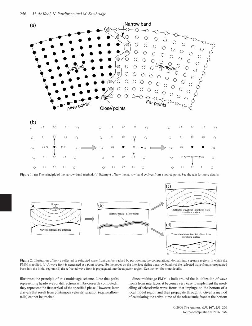
The upwind scheme given by eq. (2) describes how to calculatenew traveltimes using known traveltimes from adjacent grid points.Successful implementation of this scheme requires that the order inwhich nodes are updated be consistent with the direction of flowof information, that is, from smaller values of T to larger valuesof T . To achieve this, FMM systematically constructs traveltimes Tin a downwind fashion from known values upwind by employing anarrow-band approach. The narrow-band concept is illustrated inFig. 1(a), which for simplicity is restricted to a 2-D propagationgrid rather than the full 3-D case which is harder to visualize. Alivepoints have their values correctly calculated, close points lie withinthe narrow band and have trial values, and far points have no valuescalculated. Trial values are calculated using eq. (2) with alive pointsonly, which by definition lie upwind of the close points. The shapeof the narrow band approximates the shape of the first-arrival wavefront, and the idea is to propagate the band through the grid until allpoints become alive.

The narrow band is evolved by identifying the close point withminimum traveltime and tagging it as an alive point. All neigh-

bours of this point that are not alive are tagged as close and havetheir traveltimes computed (or recomputed) using eq. (2). Repe-tition of this process allows the traveltime to all grid points to becalculated. Fig. 1(b) illustrates several evolution steps of the narrow-band method from a source point. Choosing the close points withminimum traveltime guarantees that alive points are not evaluatedwith partial information. In general, adjacent close points must lieupwind or downwind of each other; the close point with minimumtraveltime will always lie upwind of adjacent close points.

2.2 Multistage FMM in layered media

Rawlinson & Sambridge (2004a,b) adapted the FMM scheme de-scribed above to allow phases other than the absolute first-arrivalto be tracked in layered 2-D media, with emphasis on reflectionsfrom the layer boundaries. The two principal difficulties involvedin the introduction of reflections are as follows. (i) The solution ofthe eikonal equation using the FMM yields the absolute first arrivaltime of the wave front to all points in the computational domain.To model reflected waves, the wave front has to pass through thecomputational domain at least twice. (ii) Layer boundaries that varywith depth generally do not conform to the regular velocity grid,and can thus not be accurately represented.

The problem of the representation of layer boundaries was solvedby the introduction of a set of irregularly positioned nodes that lieexactly on the interface that is the layer boundary. A connectivitybetween the irregular interface nodes and the regular grid nodeswas established with a local triangulation in the neighbourhood ofthe interface, and a special update procedure was used to calculatearrival times at the interface nodes from the nodes connected tothem. This procedure yields the first arrival times at all the interfacenodes.

By using a multistage FMM approach, the limitation of yieldingonly absolute first arrival times can be overcome for those laterarriving phases that are caused by the presence of discontinuities.After the first stage of propagating the wave front to the reflectinginterface, a copy of the region already traversed by the wave frontis created. This copy is treated as a part of space not yet traversedby the wave front, that is, the nodes in the copy start with a nodestatus far, except the ones on the reflecting interface that retaintheir arrival times from the first stage and start with a node statusclose, thus forming a new narrow band. In the second stage, thereflected phase is obtained by applying the FMM to the copy of theregion. The narrow band at the start of the second stage ‘surrounds’the interface and not the wave front, but causality is not breachedbecause the first-arrival reflection wave front only impinges on theinterface once at every point.

Although it is not strictly required by the causal nature of FMM,the same principle can also be applied to phases that refract at alayer boundary. In this case the arrival times of the wave front at theinterface are calculated in a first stage just as in the reflection case,but instead of propagating the wave front back into a copy of theregion from which it came, it is propagated into the region of spacethat lies on the other side of the interface. There are advantages tothis method in terms of accuracy (avoiding very large local wavefront curvature close to the interface), memory usage and programlogic.

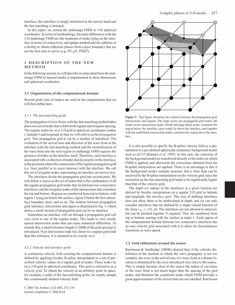
The method of reinitialization of the wave front at an interfaceoutlined above can be repeated several times to obtain the first arrivaltime of a seismic phase that is characterized by a specific sequence ofinteractions (reflections or refractions) with layer boundaries. Fig. 2

C© 2006 The Authors, GJI, 167, 253–270



Close points

Narrow band

Alive points Far points

Upwind Downwind

(b)

(a)

Figure 1. (a) The principle of the narrow-band method. (b) Example of how the narrow band evolves from a source point. See the text for more details.

Narrow band of Close points traveltime surfaceReflected wavefront initialized from

traveltime surfaceTransmitted wavefront initialized from

Wavefront tracked to interface

Source )b()a(

(c)

(d)

Figure 2. Illustration of how a reflected or refracted wave front can be tracked by partitioning the computational domain into separate regions in which theFMM is applied. (a) A wave front is generated at a point source; (b) the nodes on the interface define a narrow band; (c) the reflected wave front is propagatedback into the initial region; (d) the refracted wave front is propagated into the adjacent region. See the text for more details.

illustrates the principle of this multistage scheme. Note that pathsrepresenting headwaves or diffractions will be correctly computed ifthey represent the first arrival of the specified phase. However, laterarrivals that result from continuous velocity variation (e.g. swallow-tails) cannot be tracked.

Since multistage FMM is built around the initialization of wavefronts from interfaces, it becomes very easy to implement the mod-elling of teleseismic wave fronts that impinge on the bottom of alocal model region and then propagate through it. Given a methodof calculating the arrival time of the teleseismic front at the bottom

C© 2006 The Authors, GJI, 167, 253–270



interface, this interface is simply initialized as the narrow band andthe fast marching is initiated.

In this paper, we extend the multistage FMM to 3-D sphericalcoordinates. In terms of methodology, the main differences with the2-D multistage FMM are the treatment of nodes lying on the inter-face in terms of connectivity and update method and the addition ofa facility to obtain reflection phases from a layer boundary that arenot the first ones to arrive (e.g. PP, pP, PKKP).

3 D E S C R I P T I O N O F T H E N E WM E T H O D

In the following section we will describe in some detail how the mul-tistage FMM in layered media is implemented in three dimensionsand spherical coordinates.

3.1 Organization of the computational domain

Several grids (sets of nodes) are used in the computations that wewill first define here.

3.1.1 The fast-marching grids

The propagation of wave fronts with the fast-marching method takesplace on a set of nodes that exhibit both regular and irregular spacing.The regular nodes lie on a 3-D grid in spherical coordinates (radiusr, latitude θ and longitude φ) that we will refer to as the propagationgrid. This propagation grid is cut by a number of interfaces. Theevaluation of the arrival time and direction of the wave front at theinterface with the fast-marching method and the reinitialization ofthe wave front into the next region in multistage FMM requires thepresence of nodes on the interface itself. Therefore, each interface isassociated with a collection of nodes that lie exactly on the interface,at the positions where the connections of the regular propagation grid(i.e. lines parallel to its axes) intersect with the interface. We callthis set of irregular nodes representing an interface an intersection.

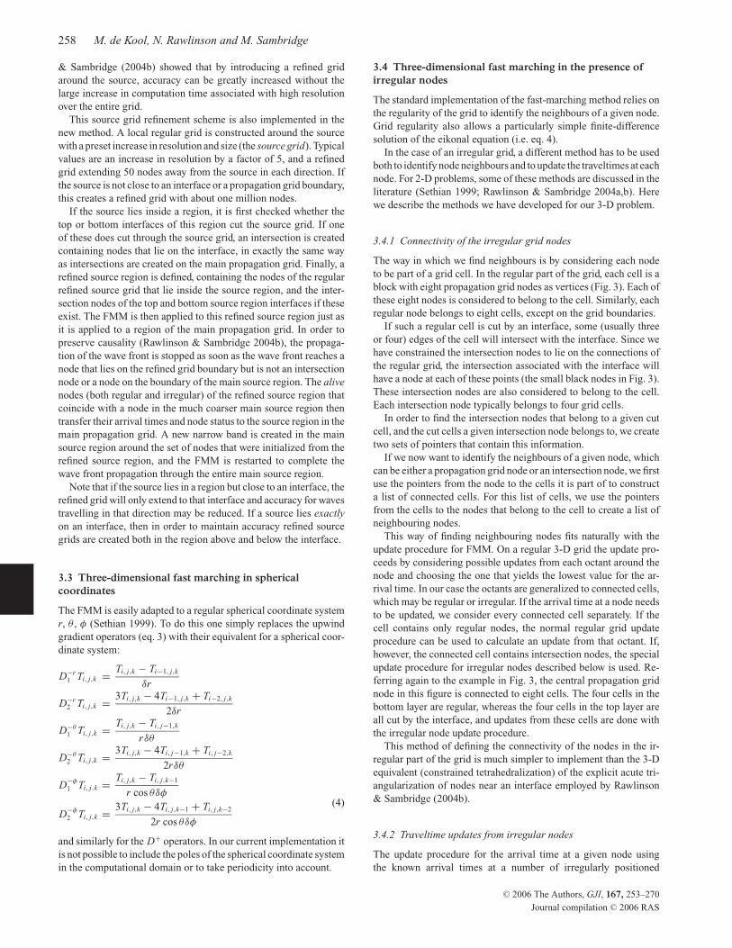
The interfaces divide the propagation grid into several parts. Wewill define a region as the set of nodes that is the combination of allthe regular propagation grid nodes that lie between two consecutiveinterfaces, and the irregular nodes of the intersections that constitutethe top and bottom. Regions are numbered from top to bottom, withregion 1 lying just below the surface, region 2 below the first subsur-face boundary layer, and so on. The relation between propagationgrid, interface, intersection and region is illustrated in Fig. 3, whichshows a small section of propagation grid cut by an interface.

Sometimes an interface will cut through a propagation grid cellvery close to one of the regular nodes. This leads to very closelyspaced intersection nodes that can cause numerical difficulties. Toremedy this, a small tolerance length (1/200th of the grid spacing) isintroduced. If an intersection node lies closer to a regular grid nodethan this tolerance, it is assumed to lie exactly on it.

3.1.2 Velocity and interface grids

A continuous velocity field covering the computational domain isdefined by applying tricubic B-spline interpolation to a set of pre-scribed velocity values on a regular grid of nodes. These nodes lieon a 3-D grid in spherical coordinates. This grid is referred to as avelocity grid. To obtain the velocity at an arbitrary point in space,for example, a node of the fast-marching grids, we simply samplethis continuously defined velocity field.

Figure 3. This figure illustrates the relation between the propagation grid,intersections and regions. The large circles are propagation grid nodes, thesmall circles intersection nodes. Small and large black nodes constitute theregion below the interface; grey nodes lie above the interface, and togetherwith the small black intersection nodes constitute the region above the inter-face.

It is also possible to specify the B-spline velocity field as a per-turbation to a pre-defined spherically symmetric background modelsuch as ak135 (Kennett et al. 1995). In this case, the velocities ofthe background model are transferred directly to the nodes on whichFMM is applied, and afterwards the corrections obtained from theB-spline interpolation are applied. There is an advantage to this ifthe background model contains structure that is finer than can beresolved by the B-spline interpolation on the velocity grid, since theresolution on the fast-marching grid tends to be significantly higherthan that of the velocity grid.

The depth (or radius) of the interfaces at a given location arederived by bicubic interpolation on a regular 2-D grid in latitudeand longitude, the interface grid. This way of defining interfacesdoes not allow them to be multivalued in depth, and we can onlyconsider interfaces that are defined by a single-valued function ofthe form r int = f (θ , φ). The interfaces are not allowed to intersect,but can be pinched together if required. They are numbered fromtop to bottom starting with the surface at index 1. Each region ofthe computational domain between two consecutive interfaces hasits own velocity grid associated with it to allow for discontinuoustransitions in wave speed.

3.2 Grid refinement around the source

Rawlinson & Sambridge (2004b) showed that, if the velocity dis-tribution in the medium in which the wave propagates is not toocomplex, the error in the arrival time of a wave front at a distant lo-cation is dominated by the error introduced very close to the source.This is simply because close to the source the radius of curvatureof the wave front is not much larger than the spacing of the gridnodes, and therefore the conditions under which FMM provides agood approximation of the arrival time are not satisfied. Rawlinson

C© 2006 The Authors, GJI, 167, 253–270



& Sambridge (2004b) showed that by introducing a refined gridaround the source, accuracy can be greatly increased without thelarge increase in computation time associated with high resolutionover the entire grid.

This source grid refinement scheme is also implemented in thenew method. A local regular grid is constructed around the sourcewith a preset increase in resolution and size (the source grid). Typicalvalues are an increase in resolution by a factor of 5, and a refinedgrid extending 50 nodes away from the source in each direction. Ifthe source is not close to an interface or a propagation grid boundary,this creates a refined grid with about one million nodes.

If the source lies inside a region, it is first checked whether thetop or bottom interfaces of this region cut the source grid. If oneof these does cut through the source grid, an intersection is createdcontaining nodes that lie on the interface, in exactly the same wayas intersections are created on the main propagation grid. Finally, arefined source region is defined, containing the nodes of the regularrefined source grid that lie inside the source region, and the inter-section nodes of the top and bottom source region interfaces if theseexist. The FMM is then applied to this refined source region just asit is applied to a region of the main propagation grid. In order topreserve causality (Rawlinson & Sambridge 2004b), the propaga-tion of the wave front is stopped as soon as the wave front reaches anode that lies on the refined grid boundary but is not an intersectionnode or a node on the boundary of the main source region. The alivenodes (both regular and irregular) of the refined source region thatcoincide with a node in the much coarser main source region thentransfer their arrival times and node status to the source region in themain propagation grid. A new narrow band is created in the mainsource region around the set of nodes that were initialized from therefined source region, and the FMM is restarted to complete thewave front propagation through the entire main source region.

Note that if the source lies in a region but close to an interface, therefined grid will only extend to that interface and accuracy for wavestravelling in that direction may be reduced. If a source lies exactlyon an interface, then in order to maintain accuracy refined sourcegrids are created both in the region above and below the interface.

3.3 Three-dimensional fast marching in sphericalcoordinates

The FMM is easily adapted to a regular spherical coordinate systemr, θ , φ (Sethian 1999). To do this one simply replaces the upwindgradient operators (eq. 3) with their equivalent for a spherical coor-dinate system:

D−r1 Ti, j,k = Ti, j,k − Ti−1, j,k

δr

D−r2 Ti, j,k = 3Ti, j,k − 4Ti−1, j,k + Ti−2, j,k

2δr

D−θ1 Ti, j,k = Ti, j,k − Ti, j−1,k

rδθ

D−θ2 Ti, j,k = 3Ti, j,k − 4Ti, j−1,k + Ti, j−2,k

2rδθ

D−φ

1 Ti, j,k = Ti, j,k − Ti, j,k−1

r cos θδφ

D−φ

2 Ti, j,k = 3Ti, j,k − 4Ti, j,k−1 + Ti, j,k−2

2r cos θδφ

(4)

and similarly for the D+ operators. In our current implementation itis not possible to include the poles of the spherical coordinate systemin the computational domain or to take periodicity into account.

3.4 Three-dimensional fast marching in the presence ofirregular nodes

The standard implementation of the fast-marching method relies onthe regularity of the grid to identify the neighbours of a given node.Grid regularity also allows a particularly simple finite-differencesolution of the eikonal equation (i.e. eq. 4).

In the case of an irregular grid, a different method has to be usedboth to identify node neighbours and to update the traveltimes at eachnode. For 2-D problems, some of these methods are discussed in theliterature (Sethian 1999; Rawlinson & Sambridge 2004a,b). Herewe describe the methods we have developed for our 3-D problem.

3.4.1 Connectivity of the irregular grid nodes

The way in which we find neighbours is by considering each nodeto be part of a grid cell. In the regular part of the grid, each cell is ablock with eight propagation grid nodes as vertices (Fig. 3). Each ofthese eight nodes is considered to belong to the cell. Similarly, eachregular node belongs to eight cells, except on the grid boundaries.

If such a regular cell is cut by an interface, some (usually threeor four) edges of the cell will intersect with the interface. Since wehave constrained the intersection nodes to lie on the connections ofthe regular grid, the intersection associated with the interface willhave a node at each of these points (the small black nodes in Fig. 3).These intersection nodes are also considered to belong to the cell.Each intersection node typically belongs to four grid cells.

In order to find the intersection nodes that belong to a given cutcell, and the cut cells a given intersection node belongs to, we createtwo sets of pointers that contain this information.

If we now want to identify the neighbours of a given node, whichcan be either a propagation grid node or an intersection node, we firstuse the pointers from the node to the cells it is part of to constructa list of connected cells. For this list of cells, we use the pointersfrom the cells to the nodes that belong to the cell to create a list ofneighbouring nodes.

This way of finding neighbouring nodes fits naturally with theupdate procedure for FMM. On a regular 3-D grid the update pro-ceeds by considering possible updates from each octant around thenode and choosing the one that yields the lowest value for the ar-rival time. In our case the octants are generalized to connected cells,which may be regular or irregular. If the arrival time at a node needsto be updated, we consider every connected cell separately. If thecell contains only regular nodes, the normal regular grid updateprocedure can be used to calculate an update from that octant. If,however, the connected cell contains intersection nodes, the specialupdate procedure for irregular nodes described below is used. Re-ferring again to the example in Fig. 3, the central propagation gridnode in this figure is connected to eight cells. The four cells in thebottom layer are regular, whereas the four cells in the top layer areall cut by the interface, and updates from these cells are done withthe irregular node update procedure.

This method of defining the connectivity of the nodes in the ir-regular part of the grid is much simpler to implement than the 3-Dequivalent (constrained tetrahedralization) of the explicit acute tri-angularization of nodes near an interface employed by Rawlinson& Sambridge (2004b).

3.4.2 Traveltime updates from irregular nodes

The update procedure for the arrival time at a given node usingthe known arrival times at a number of irregularly positioned

C© 2006 The Authors, GJI, 167, 253–270



neighbouring nodes is based on making the assumption that thewave front can be approximated locally as planar, and using the val-ues of the arrival times at the neighbours to obtain the best possibleestimate of the wave front normal that is certain not to underestimatethe arrival time T u at the updated node. The assumption of a planewave front means that this method is of first order, and hence isgenerally not as accurate as the second-order schemes that are eas-ily applied to regular grids. This does not have a significant impacton the overall accuracy of the results, however, since the irregularupdate method is only used in the direct vicinity of the interfacesthat are described by irregular nodes. Since a plane wave approx-imation is much more easily applied in Cartesian coordinates, wefirst convert the positions of the nodes used for an irregular updateto a local Cartesian coordinate system. A second-order method isused for the updates from regular connected cells.

To first order, the difference in arrival times δT between twopoints with relative position δx is given by

δT = ∇T · δx. (5)

By definition, ∇T ≡ sn, where n is the wave front normal. Thearrival time update procedure for irregular cells essentially consistsof solving the finite-difference form of eq. (5). When updating ar-rival times using information from the alive nodes that are part of anirregular connected cell, the number of alive nodes in that cell canbe either 1, 2, 3 or >3. If the arrival times are known at exactly threeneighbouring nodes, these times define a unique plane wave thatcan be calculated and then used to find the arrival time at the updatenode. When only one or two nodes are available, extra constraintshave to be added to find a solution for the plane wave, and whenmore than three nodes are available there is redundant information.We consider these four cases separately.

To calculate the update to the arrival time at a node where thearrival times are known at three neighbouring nodes, say, T 1, T 2,T 3 at positions x1, x2, x3, the updated time is found by solving theset of equations

T2 − T1 = s12n · (x2 − x1)

T3 − T1 = s13n · (x3 − x1)

|n| = 1 (6)

for the wave front normal n. Here s12 and s13 represent the aver-age slowness between points 1 and 2 and 1 and 3, respectively. Thefirst equation constrains the wave front to have a certain angle withrespect to the line connecting points 1 and 2; the second gives a con-straint on the angle between the wave front and the line connectingpoints 1 and 3. Once n is known, the updated arrival time T u at xu

can be found from

Tu = T1 + s1un · (xu − x1). (7)

An additional constraint has to be applied to the solution (Sethian1999) to ensure the causality of the update method: the update musttake place from a direction that is contained within the solid anglesubtended by the triangle formed by the three nodes with knownarrival time as seen from the node that is updated. If the vector −n,where n is the solution of eq. (6), lies outside this solid angle theestimated arrival time calculated is rejected. Note that the enforce-ment of acute triangulation of nodes in the interface neighbourhoodemployed by Rawlinson & Sambridge (2004a) is a way of ensuringthis causality, and obviates the need for an explicit causality test.

If only two neighbouring nodes have known arrival times, thewave front normal is not uniquely defined by the known nodes. Anextra constraint on the wave front normal is added, ensuring that

the updated arrival time is an upper limit, which is geometricallyequivalent to the constraint that the wave front normal lies in theplane that contains the two known nodes and the node to be updated.The set of equations for n in this case is

T2 − T1 = s12n · (x2 − x1)

0 = n · [(x2 − xu) × (x1 − xu)]

|n| = 1. (8)

Again a causality test has to be applied to the solution: in the planethat contains the two known nodes and the node to be updated, −nmust lie within the angle subtended by the two known nodes as seenfrom the update point.

If only a single known node neighbours an update node, the upperlimit on the arrival time at the update node is simply derived bymultiplying the distance with the slowness:

Tu = T1 + s1u |(xu − x1)|. (9)

No causality check is required when updating from a single knownneighbouring node.

Because of the partial regularity of the set of nodes on which thewave front propagation is calculated, it frequently occurs that for athree-node update the three known nodes and the update node arecoplanar. In this case, the three-node update procedure will fail, anda two-node update has to be applied instead.

If a connected cell contains more than three nodes with knownarrival times, we simply consider all possible combinations of knownnodes in single node, two-node and three-node update mode. It isnot possible to consider only three-node combinations since thecausality test may reject all such solutions, and the best (and onlyallowable) solution may be a single-node one. Potentially the numberof combinations can be very large: m + 2C m + 3C m where i C j isthe number of different combinations of i objects that can be formedout of a set of j objects, and m is the number of alive nodes in theconnected cell. It is, however, significantly reduced to m + 2C m−1

if one makes use of the causal nature of the fast-marching method,which ensures that any update from a combination of nodes that doesnot contain the node that most recently became alive has alreadybeen performed and does not have to be repeated.

3.5 Path sequences in multistage FMM

As outlined above, the multistage fast-marching method consistsof finding fast-marching solutions to the traveltime field for a se-quence of regions between interfaces. The first step in the sequencecalculates the traveltime field in the region in which the source islocated, or in the regions above and below it if the source is exactlylocated on an interface. Each consecutive step in the sequence takesthe nodes and associated arrival times of either the top or bottomintersections of the region from the previous step in the sequence asthe initial narrow band for the fast-marching wave front propagationinto the next region. If the front is propagated back into the sameregion as the previous step in the sequence, it represents a reflectionfrom the interface. If the front propagates into a region adjacent tothe region of the previous step, it represents a refraction. This isillustrated schematically in Fig. 4.

A specific later arriving phase or path (we use these terms inter-changeably) to be computed is defined as a sequence of interfacesand propagation directions. We can represent each step in such asequence with a naming convention of the form P nm, where n is thestarting interface and m is the region in which the propagation takesplace. For example, propagation of the wave front from interface

C© 2006 The Authors, GJI, 167, 253–270



region 1

region 2

path 2

path 3

path 1

interface 2

interface 1

interface 3

Path sequences

01

01

22

22

01 22 32 21

21

32 22 2132

path 1: P P P P

path 2: P P P

path 3: P P P P P P

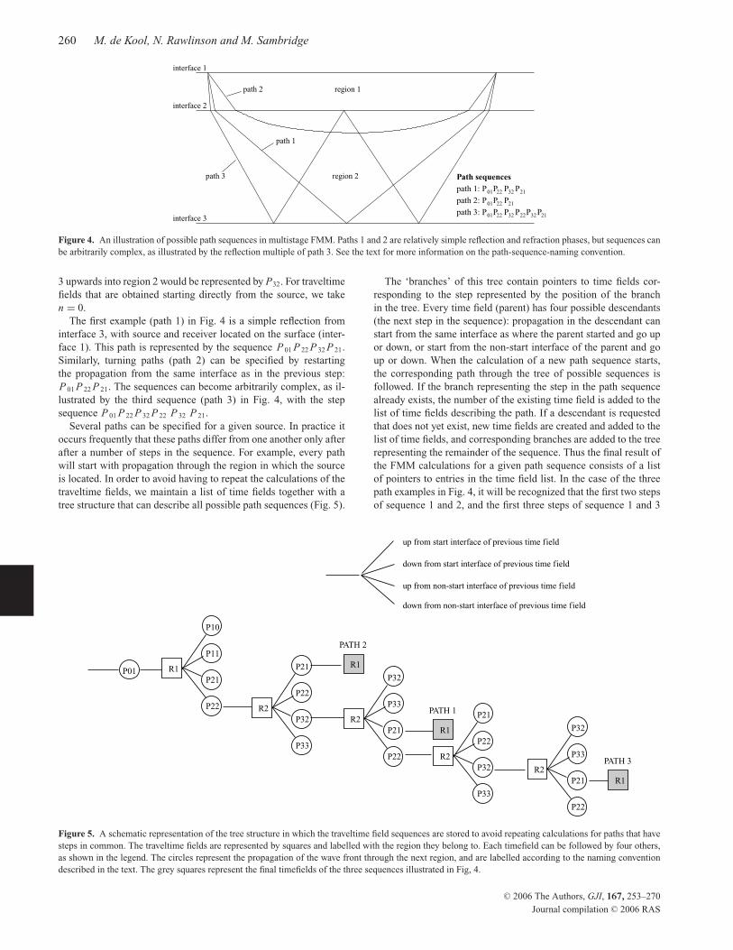
Figure 4. An illustration of possible path sequences in multistage FMM. Paths 1 and 2 are relatively simple reflection and refraction phases, but sequences canbe arbitrarily complex, as illustrated by the reflection multiple of path 3. See the text for more information on the path-sequence-naming convention.

3 upwards into region 2 would be represented by P32. For traveltimefields that are obtained starting directly from the source, we taken = 0.

The first example (path 1) in Fig. 4 is a simple reflection frominterface 3, with source and receiver located on the surface (inter-face 1). This path is represented by the sequence P 01 P 22 P 32 P 21.Similarly, turning paths (path 2) can be specified by restartingthe propagation from the same interface as in the previous step:P 01 P 22 P 21. The sequences can become arbitrarily complex, as il-lustrated by the third sequence (path 3) in Fig. 4, with the stepsequence P 01 P 22 P 32 P 22 P 32 P 21.

Several paths can be specified for a given source. In practice itoccurs frequently that these paths differ from one another only afterafter a number of steps in the sequence. For example, every pathwill start with propagation through the region in which the sourceis located. In order to avoid having to repeat the calculations of thetraveltime fields, we maintain a list of time fields together with atree structure that can describe all possible path sequences (Fig. 5).

PATH 1

PATH 3

PATH 2

P01

P22

P10

P32

P22

P32

P33

P21

P22P32

down from non-start interface of previous time field

up from start interface of previous time field

P11

up from non-start interface of previous time field

down from start interface of previous time field

R1P21

P33

P21

P22

R1

R1

R2

R2

R2R2

P22

P21

P33

P32

P33

P21

R1

Figure 5. A schematic representation of the tree structure in which the traveltime field sequences are stored to avoid repeating calculations for paths that havesteps in common. The traveltime fields are represented by squares and labelled with the region they belong to. Each timefield can be followed by four others,as shown in the legend. The circles represent the propagation of the wave front through the next region, and are labelled according to the naming conventiondescribed in the text. The grey squares represent the final timefields of the three sequences illustrated in Fig, 4.

The ‘branches’ of this tree contain pointers to time fields cor-responding to the step represented by the position of the branchin the tree. Every time field (parent) has four possible descendants(the next step in the sequence): propagation in the descendant canstart from the same interface as where the parent started and go upor down, or start from the non-start interface of the parent and goup or down. When the calculation of a new path sequence starts,the corresponding path through the tree of possible sequences isfollowed. If the branch representing the step in the path sequencealready exists, the number of the existing time field is added to thelist of time fields describing the path. If a descendant is requestedthat does not yet exist, new time fields are created and added to thelist of time fields, and corresponding branches are added to the treerepresenting the remainder of the sequence. Thus the final result ofthe FMM calculations for a given path sequence consists of a listof pointers to entries in the time field list. In the case of the threepath examples in Fig. 4, it will be recognized that the first two stepsof sequence 1 and 2, and the first three steps of sequence 1 and 3

C© 2006 The Authors, GJI, 167, 253–270



P

pP PP

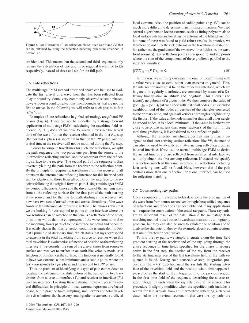
Figure 6. An illustration of late reflection phases such as pP and PP thatcan be obtained by using the reflection matching procedure described inSection 3.6.

are identical. This means that the second and third sequences onlyrequire the calculation of one and three regional traveltime fieldsrespectively, instead of three and six for the full path.

3.6 Late reflections

The multistage FMM method described above can be used to eval-uate the first arrival of a wave front that has been reflected froma layer boundary. Some very commonly observed seismic phases,however, correspond to reflections from boundaries that are not thefirst to arrive. In the following we will refer to such phases as latereflections.

Examples of late reflections in global seismology are pP and PPphases (Fig. 6). These can not be modelled by a straightforwardapplication of multistage FMM: calculating the traveltime field se-quence P 01 P 11 does not yield the PP arrival time since the arrivaltime of the wave front at the receiver obtained in the first P01 step(the normal P phase) is shorter than that of the PP phase, and thearrival time at the receiver will not be modified during the P11 step.

In order to compute traveltimes for such late reflections, we splitthe path sequence into two parts: one part from the source to theintermediate reflecting surface, and the other part from the reflect-ing surface to the receiver. The second part of the sequence is theninverted, yielding the path from the receiver to the reflection point.By the principle of reciprocity, traveltimes from the receiver to allpoints on the intermediate reflecting interface for this inverted pathwill be identical to those from all points on the interface to the re-ceiver following the original forward path. Using (multistage) FMMwe compute the arrival times and the directions of the arriving wavefront at the reflecting surface for the first part of the path startingat the source, and for the inverted path starting at the receiver. Wenow have two sets of arrival times and arrival directions of the wavefronts at the intermediate reflecting surface. The phases (rays) thatwe are looking for correspond to points on the interface where thetwo solutions can be matched so that one is a reflection of the other,or in other words that the components of the wave front normal tothe incoming fronts parallel to the interface are equal and opposite.It is easily shown that this reflection condition is equivalent to Fer-mat’s principle of stationary time, which states that rays correspondto extrema in the total traveltime from source to receiver when thistotal traveltime is evaluated as a function of position on the reflectinginterface. If we consider the sum of the arrival times from source tosurface and receiver to surface in an earth-like velocity model as afunction of position on the surface, this function is generally foundto have two extrema, a local minimum and a saddle point, where thefirst corresponds to a pP phase and the second to a PP phase.

Thus the problem of identifying this type of path comes down tolocating the extrema in the distribution of the sum of the two trav-eltimes from source to interface (T s) and receiver to interface (T r)over an interface. Locating these extrema, however, presents sev-eral difficulties. In principle all local extrema represent a reflectedphase, but in practice finite sampling, small errors and total travel-time distributions that have very small gradients can create artificial

local extrema. Also, the position of saddle points (e.g. PP) can bemuch more difficult to determine than minima or maxima. We triedseveral algorithms to locate extrema, such as fitting polynomials tolocal surface patches and locating the extrema of the fitting function,but none of these was found to yield robust results. In practice, wetherefore do not directly seek extrema in the traveltime distribution,but rather use the gradients of the two traveltime fields (i.e. the wavefront normals). The reflection points correspond to surface pointswhere the sum of the components of these gradients parallel to theinterface vanishes:∣∣(∇Ts)|| + (∇Tr)||

∣∣ = 0. (10)

In this way, we simplify our search to one for local minima witha value very close to zero, rather than extrema in general. First,the intersection nodes that lie on the reflecting interface, which arein general irregularly distributed, are connected by means of a De-launay triangulation in latitude and longitude. This allows us toidentify neighbours of a given node. We then compare the value of|(∇T s)|| + (∇T r)||| at each node with that of all nodes in an extendedneighbourhood of the node: all vertices of the triangles connectedto the primary node, and again all vertices of triangles neighbouringthe first set. If the value at the node is smaller than at all other neigh-bourhood nodes, it is a local minimum. If the value is furthermoreclose to zero, that is, less than some fraction ε of the norm of thetotal time gradient s, it is considered to be a reflection point.

Although the reflection matching algorithm was primarily de-signed to find later arriving surface reflections like PP, the methodcan also be used to identify any later arriving reflection from aninternal interface. If we use the normal multistage FMM to derivethe arrival time of a phase reflected from an internal interface wewill only obtain the first arriving reflection. If instead we specifya reflection match at the same interface, all reflections includinglater arriving ones will be found. Note, however, that if the pathcontains more than one reflection, only one interface can be usedfor reflection matching.

3.7 Constructing ray paths

Once a sequence of traveltime fields describing the propagation ofthe wave front from source to receiver through the specified sequenceof refractions and reflections has been obtained, many applicationswill require the construction of the actual ray paths. These ray pathsare an important result of the calculation if the multistage fast-marching method is used as the forward step in a seismic tomographyproblem, but they can also be used to validate the solution and toanalyse the character of the ray, for example, does it contain sectionsthat are diffracted or head waves.

To find the ray paths, we simply integrate along the time fieldgradient starting at the receiver end of the ray, going through theentire sequence of time fields specified for the phase in reverseorder. In the first step, the section of the ray from the receiverto the starting interface of the last traveltime field in the path se-quence is found. During each consecutive step, integration pro-ceeds in the −∇T direction until the ray hits the starting inter-face of the traveltime field, and the position where this happens ispassed on as the start of the integration into the previous region.In the first time field of the sequence, describing the source re-gion, integration ends when the ray gets close to the source. Thisprocedure is slightly modified when the specified path includes asearch for late arrivals from an intermediate reflecting surface asdescribed in the previous section: in that case the ray paths are

C© 2006 The Authors, GJI, 167, 253–270



determined by starting at each reflection point found, and integrat-ing down the time field gradient both towards the source and thereceiver.

To integrate along the gradient of a traveltime field, the first stepis the evaluation of the gradient itself. The normal FMM only yieldsthe arrival time at each node of the grid, and for the integrationwe need the gradient of this field. On internal nodes of the regu-lar grid (i.e. nodes that have neighbours in all six principal direc-tions), the gradient can be easily derived by finite differencing. Onthe boundaries of the grid, however, we encounter two problems.The first is that we can only take one-sided differences in the di-rections crossing the interface, which can lead to quite significanterrors in the gradient at the nodes on the interface. The second isthat the intersection nodes are irregularly positioned. We have there-fore taken the approach of storing the traveltime gradient at eachnode explicitly during the fast-marching calculations. The travel-time gradient at a node is given by a vector with a direction equal tothe normal to the wave front used for the final update of the arrivaltime at the node, and a norm that is the local slowness. This ap-proach significantly improves the accuracy of the ray paths near theinterfaces.

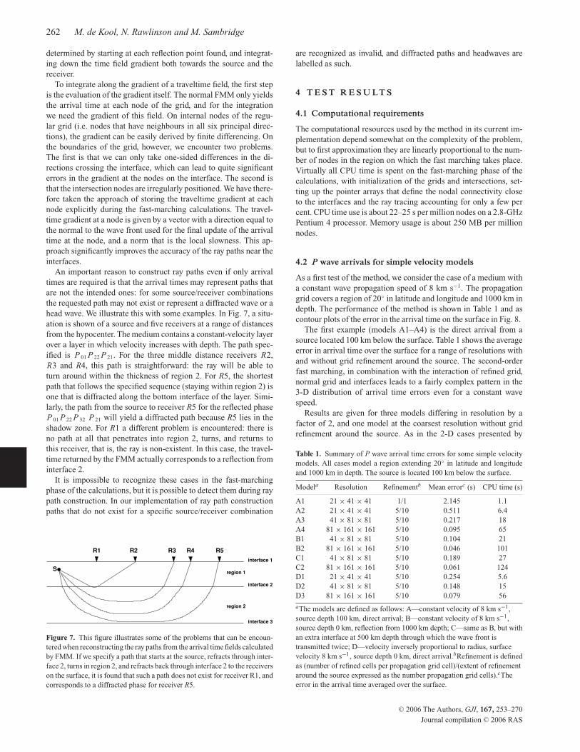
An important reason to construct ray paths even if only arrivaltimes are required is that the arrival times may represent paths thatare not the intended ones: for some source/receiver combinationsthe requested path may not exist or represent a diffracted wave or ahead wave. We illustrate this with some examples. In Fig. 7, a situ-ation is shown of a source and five receivers at a range of distancesfrom the hypocenter. The medium contains a constant-velocity layerover a layer in which velocity increases with depth. The path spec-ified is P 01 P 22 P 21. For the three middle distance receivers R2,R3 and R4, this path is straightforward: the ray will be able toturn around within the thickness of region 2. For R5, the shortestpath that follows the specified sequence (staying within region 2) isone that is diffracted along the bottom interface of the layer. Simi-larly, the path from the source to receiver R5 for the reflected phaseP 01 P 22 P 32 P 21 will yield a diffracted path because R5 lies in theshadow zone. For R1 a different problem is encountered: there isno path at all that penetrates into region 2, turns, and returns tothis receiver, that is, the ray is non-existent. In this case, the travel-time returned by the FMM actually corresponds to a reflection frominterface 2.

It is impossible to recognize these cases in the fast-marchingphase of the calculations, but it is possible to detect them during raypath construction. In our implementation of ray path constructionpaths that do not exist for a specific source/receiver combination

region 2

region 1

interface 3

interface 1

interface 2

R3

S

R2 R4 R5R1

Figure 7. This figure illustrates some of the problems that can be encoun-tered when reconstructing the ray paths from the arrival time fields calculatedby FMM. If we specify a path that starts at the source, refracts through inter-face 2, turns in region 2, and refracts back through interface 2 to the receiverson the surface, it is found that such a path does not exist for receiver R1, andcorresponds to a diffracted phase for receiver R5.

are recognized as invalid, and diffracted paths and headwaves arelabelled as such.

4 T E S T R E S U LT S

4.1 Computational requirements

The computational resources used by the method in its current im-plementation depend somewhat on the complexity of the problem,but to first approximation they are linearly proportional to the num-ber of nodes in the region on which the fast marching takes place.Virtually all CPU time is spent on the fast-marching phase of thecalculations, with initialization of the grids and intersections, set-ting up the pointer arrays that define the nodal connectivity closeto the interfaces and the ray tracing accounting for only a few percent. CPU time use is about 22–25 s per million nodes on a 2.8-GHzPentium 4 processor. Memory usage is about 250 MB per millionnodes.

4.2 P wave arrivals for simple velocity models

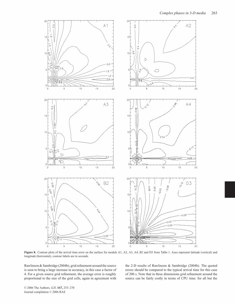
As a first test of the method, we consider the case of a medium witha constant wave propagation speed of 8 km s−1. The propagationgrid covers a region of 20◦ in latitude and longitude and 1000 km indepth. The performance of the method is shown in Table 1 and ascontour plots of the error in the arrival time on the surface in Fig. 8.

The first example (models A1–A4) is the direct arrival from asource located 100 km below the surface. Table 1 shows the averageerror in arrival time over the surface for a range of resolutions withand without grid refinement around the source. The second-orderfast marching, in combination with the interaction of refined grid,normal grid and interfaces leads to a fairly complex pattern in the3-D distribution of arrival time errors even for a constant wavespeed.

Results are given for three models differing in resolution by afactor of 2, and one model at the coarsest resolution without gridrefinement around the source. As in the 2-D cases presented by

Table 1. Summary of P wave arrival time errors for some simple velocitymodels. All cases model a region extending 20◦ in latitude and longitudeand 1000 km in depth. The source is located 100 km below the surface.

Modela Resolution Refinementb Mean errorc (s) CPU time (s)

A1 21 × 41 × 41 1/1 2.145 1.1A2 21 × 41 × 41 5/10 0.511 6.4A3 41 × 81 × 81 5/10 0.217 18A4 81 × 161 × 161 5/10 0.095 65B1 41 × 81 × 81 5/10 0.104 21B2 81 × 161 × 161 5/10 0.046 101C1 41 × 81 × 81 5/10 0.189 27C2 81 × 161 × 161 5/10 0.061 124D1 21 × 41 × 41 5/10 0.254 5.6D2 41 × 81 × 81 5/10 0.148 15D3 81 × 161 × 161 5/10 0.079 56

aThe models are defined as follows: A—constant velocity of 8 km s−1,source depth 100 km, direct arrival; B—constant velocity of 8 km s−1,source depth 0 km, reflection from 1000 km depth; C—same as B, but withan extra interface at 500 km depth through which the wave front istransmitted twice; D—velocity inversely proportional to radius, surfacevelocity 8 km s−1, source depth 0 km, direct arrival.bRefinement is definedas (number of refined cells per propagation grid cell)/(extent of refinementaround the source expressed as the number propagation grid cells).cTheerror in the arrival time averaged over the surface.

C© 2006 The Authors, GJI, 167, 253–270



Figure 8. Contour plots of the arrival time error on the surface for models A1, A2, A3, A4, B2 and D3 from Table 1. Axes represent latitude (vertical) andlongitude (horizontal), contour labels are in seconds.

Rawlinson & Sambridge (2004b), grid refinement around the sourceis seen to bring a large increase in accuracy, in this case a factor of4. For a given source grid refinement, the average error is roughlyproportional to the size of the grid cells, again in agreement with

the 2-D results of Rawlinson & Sambridge (2004b). The quotederrors should be compared to the typical arrival time for this caseof 200 s. Note that in three dimensions grid refinement around thesource can be fairly costly in terms of CPU time: for all but the

C© 2006 The Authors, GJI, 167, 253–270



highest resolution model (81 × 161 × 161) the refined grid aroundthe source contains many more nodes than the main propagationgrid, which accounts for the CPU times listed for each model inTable 1.

The second example (models B1–B2) calculates the arrival timeof the reflection from a layer at 1000 km depth from a source ly-ing on the surface. This involves first propagating the wave frontthrough the grid to the bottom interface, re-initializing the fastmarching from the bottom interface and propagating back to thesurface. The errors for this case are about half those in the directarrival from a 100 km deep source. We attribute the smaller error tothe fact that the wave front hits the interfaces at a much steeperangle and with less curvature. Thereby the effect of the lower-accuracy (first-order) layer directly adjacent to the interfaces isreduced.

In the third example (models C1–C2) we investigate the effect onaccuracy of traversing an interface (refraction). We keep the velocityconstant, but introduce an extra interface at 500 km depth. Thisshould give the same result as the previous example, but stoppingand restarting from the intermediate interface both on the way downand on the way up will obviously introduce additional errors. Forthe 41 × 81 × 81 grid, the error increases by 80 per cent, for thefiner resolution of 81 × 161 × 161 by 30 per cent.

The next three models (D1–D3) address the slightly more com-plex case of velocity increasing with depth. We choose the casev = v0 R0/r where v0 is the velocity at the surface and R0 the ra-dius of the earth. The traveltime between two points on the surfacein this model is given by t = R0 sin �/v0, with � the angular dis-tance between the two points. In order to use this simple analyticalresult, the source is positioned at the surface.

The average arrival time errors at the surface are smaller thanin the constant-velocity case. Again we attribute this to the factthat a smaller fraction of each ray path lies in the first-order layeradjacent to the surface because the velocity gradient bends the raypath inward.

4.3 P wave traveltimes in the ak135 reference model

The next model we consider is considerably more complex than theprevious cases for which analytical solutions are available. The ve-locity structure is assumed to be given by the ak135 reference model(Kennett et al. 1995). Accurate tables of arrival times in this 1-Dmodel are available to compare with our solutions. P wave veloc-ity discontinuities at 20, 35, 410 and 660 km depth are explicitlyrepresented by interfaces as described in the previous section, andbetween these interfaces the velocity at the nodes is derived by lin-ear interpolation from the ak135 velocity tables. In order to avoidthe errors being dominated by the sampling of the velocity grids,the spacing of the velocity grid nodes was reduced from the usualcase of four times the propagation grid node spacing to two timesthe propagation grid node spacing. The region modelled is the samesize as in the previous examples, that is, 20◦ in latitude and 20◦ inlongitude.

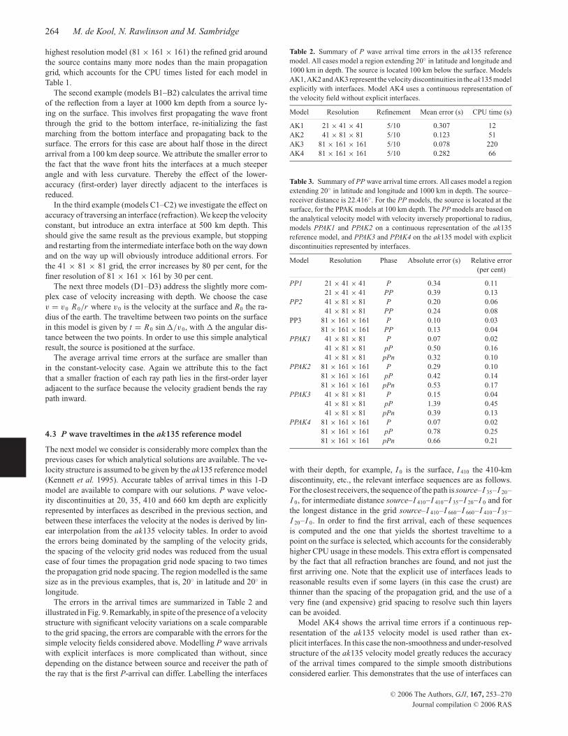
The errors in the arrival times are summarized in Table 2 andillustrated in Fig. 9. Remarkably, in spite of the presence of a velocitystructure with significant velocity variations on a scale comparableto the grid spacing, the errors are comparable with the errors for thesimple velocity fields considered above. Modelling P wave arrivalswith explicit interfaces is more complicated than without, sincedepending on the distance between source and receiver the path ofthe ray that is the first P-arrival can differ. Labelling the interfaces

Table 2. Summary of P wave arrival time errors in the ak135 referencemodel. All cases model a region extending 20◦ in latitude and longitude and1000 km in depth. The source is located 100 km below the surface. ModelsAK1, AK2 and AK3 represent the velocity discontinuities in the ak135 modelexplicitly with interfaces. Model AK4 uses a continuous representation ofthe velocity field without explicit interfaces.

Model Resolution Refinement Mean error (s) CPU time (s)

AK1 21 × 41 × 41 5/10 0.307 12AK2 41 × 81 × 81 5/10 0.123 51AK3 81 × 161 × 161 5/10 0.078 220AK4 81 × 161 × 161 5/10 0.282 66

Table 3. Summary of PP wave arrival time errors. All cases model a regionextending 20◦ in latitude and longitude and 1000 km in depth. The source–receiver distance is 22.416◦. For the PP models, the source is located at thesurface, for the PPAK models at 100 km depth. The PP models are based onthe analytical velocity model with velocity inversely proportional to radius,models PPAK1 and PPAK2 on a continuous representation of the ak135reference model, and PPAK3 and PPAK4 on the ak135 model with explicitdiscontinuities represented by interfaces.

Model Resolution Phase Absolute error (s) Relative error(per cent)

PP1 21 × 41 × 41 P 0.34 0.1121 × 41 × 41 PP 0.39 0.13

PP2 41 × 81 × 81 P 0.20 0.0641 × 81 × 81 PP 0.24 0.08

PP3 81 × 161 × 161 P 0.10 0.0381 × 161 × 161 PP 0.13 0.04

PPAK1 41 × 81 × 81 P 0.07 0.0241 × 81 × 81 pP 0.50 0.1641 × 81 × 81 pPn 0.32 0.10

PPAK2 81 × 161 × 161 P 0.29 0.1081 × 161 × 161 pP 0.42 0.1481 × 161 × 161 pPn 0.53 0.17

PPAK3 41 × 81 × 81 P 0.15 0.0441 × 81 × 81 pP 1.39 0.4541 × 81 × 81 pPn 0.39 0.13

PPAK4 81 × 161 × 161 P 0.07 0.0281 × 161 × 161 pP 0.78 0.2581 × 161 × 161 pPn 0.66 0.21

with their depth, for example, I 0 is the surface, I 410 the 410-kmdiscontinuity, etc., the relevant interface sequences are as follows.For the closest receivers, the sequence of the path is source–I 35–I 20–I 0, for intermediate distance source–I 410–I 410–I 35–I 20–I 0 and forthe longest distance in the grid source–I 410–I 660–I 660–I 410–I 35–I 20–I 0. In order to find the first arrival, each of these sequencesis computed and the one that yields the shortest traveltime to apoint on the surface is selected, which accounts for the considerablyhigher CPU usage in these models. This extra effort is compensatedby the fact that all refraction branches are found, and not just thefirst arriving one. Note that the explicit use of interfaces leads toreasonable results even if some layers (in this case the crust) arethinner than the spacing of the propagation grid, and the use of avery fine (and expensive) grid spacing to resolve such thin layerscan be avoided.

Model AK4 shows the arrival time errors if a continuous rep-resentation of the ak135 velocity model is used rather than ex-plicit interfaces. In this case the non-smoothness and under-resolvedstructure of the ak135 velocity model greatly reduces the accuracyof the arrival times compared to the simple smooth distributionsconsidered earlier. This demonstrates that the use of interfaces can

C© 2006 The Authors, GJI, 167, 253–270



Figure 9. Contour plots of P wave arrival time error on the surface for models AK1–AK4 from Table 2. Axes represent latitude (vertical) and longitude(horizontal), contour labels are in seconds.

greatly reduce the error for a given propagation grid spacing com-pared to the case when the same velocity distribution is representedas a continuous velocity field. The reduction in error can be at-tributed to two effects. The first is the accurate representation ofthe position of the interface. The second is that because the wavefront propagation by fast marching proceeds on a region-by-regionbasis, the wave front never passes over the abrupt changes in thevelocity distribution. Propagating a wave front over such abruptchanges in velocity with fast marching can lead to the introductionof errors that are significantly larger than those for smooth velocitydistributions.

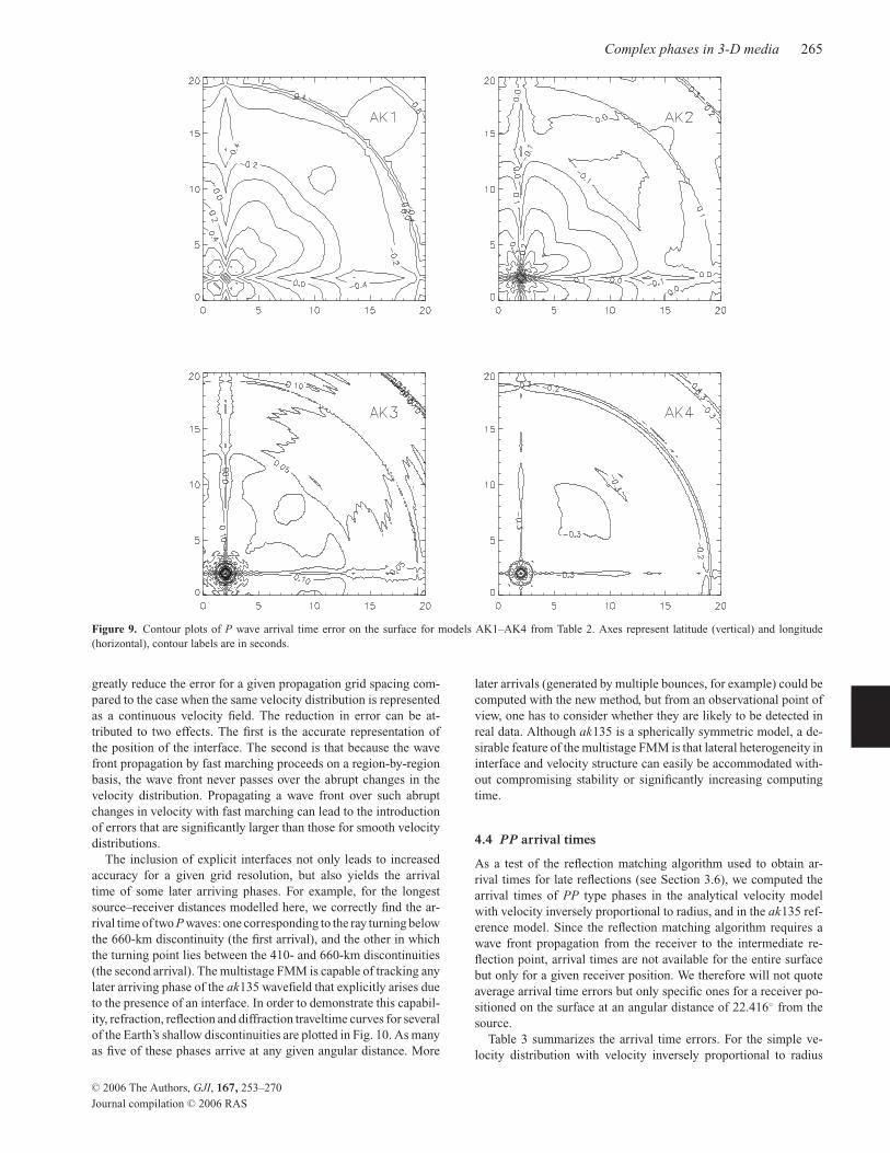
The inclusion of explicit interfaces not only leads to increasedaccuracy for a given grid resolution, but also yields the arrivaltime of some later arriving phases. For example, for the longestsource–receiver distances modelled here, we correctly find the ar-rival time of two P waves: one corresponding to the ray turning belowthe 660-km discontinuity (the first arrival), and the other in whichthe turning point lies between the 410- and 660-km discontinuities(the second arrival). The multistage FMM is capable of tracking anylater arriving phase of the ak135 wavefield that explicitly arises dueto the presence of an interface. In order to demonstrate this capabil-ity, refraction, reflection and diffraction traveltime curves for severalof the Earth’s shallow discontinuities are plotted in Fig. 10. As manyas five of these phases arrive at any given angular distance. More

later arrivals (generated by multiple bounces, for example) could becomputed with the new method, but from an observational point ofview, one has to consider whether they are likely to be detected inreal data. Although ak135 is a spherically symmetric model, a de-sirable feature of the multistage FMM is that lateral heterogeneity ininterface and velocity structure can easily be accommodated with-out compromising stability or significantly increasing computingtime.

4.4 PP arrival times

As a test of the reflection matching algorithm used to obtain ar-rival times for late reflections (see Section 3.6), we computed thearrival times of PP type phases in the analytical velocity modelwith velocity inversely proportional to radius, and in the ak135 ref-erence model. Since the reflection matching algorithm requires awave front propagation from the receiver to the intermediate re-flection point, arrival times are not available for the entire surfacebut only for a given receiver position. We therefore will not quoteaverage arrival time errors but only specific ones for a receiver po-sitioned on the surface at an angular distance of 22.416◦ from thesource.

Table 3 summarizes the arrival time errors. For the simple ve-locity distribution with velocity inversely proportional to radius

C© 2006 The Authors, GJI, 167, 253–270



0 5 10 15 20 25 30 3510

15

20

25

30

35

40

45

50

55

60

Pn

P

P

Pdiff(410)

Pdiff(660)

P(410)P

P(660)P

∆ (angular distance) [degrees]

∆ [s

eco

nd

s]

Figure 10. Traveltime curves computed by the multistage FMM for various phases that occur as a result of several of the Earth’s shallow discontinuities (theMoho and 410 and 660 discontinuities), as defined by the global reference model ak135. Dashed lines represent reflections from the 410 and 660 discontinuities;these become diffractions at larger angular distances. The source is located on the surface of the Earth.

(PP1–PP3), the errors are only slightly larger than the directP-arrivals, which is quite good considering the fact that it involvesfinding the reflection point and performing two independent wavefront propagations whose errors will be superimposed.

For the models based on the ak135 reference model (PPAK1–PPAK4), the errors are quite variable, but can be understood asfollows. Consider first only the errors in the direct P-arrivals. Inthe models with continuous velocity representation, the total errorin arrival time is both due to a poor representation of the model(unavoidable because of the coarse grid spacing compared to thestructure in the ak135 model near the surface), and due to errorsinduced by second-order FMM when the velocity distribution isvery non-smooth on the scale of the grid resolution. By coincidence,these errors tend to cancel each other out (for the specific geometryconsidered) at a grid resolution of 25 km in the radial direction (41× 81 × 81), leading to quite small errors in the direct P-arrival. Thatthis is the case can be seen from the result of the model with twicethe resolution, for which the direct P-arrival error is much largerinstead of smaller. By contrast, in the velocity model representing thediscontuities with explicit interfaces the errors converge as expectedwith an increase in grid resolution.

The ray paths of the pP and pPn phases are more complex andlie closer to the surface. In the continuous velocity models, thisleads to an increase in error by a factor of about 2. The large errorsfor the pP and pPn phases in the discontinuous velocity model aredue to a limitation in our current implementation of the method:the grid refinement around the source is limited to the region inwhich the source lies. In the layered ak135 model, the propagation

of the wave front from the receiver to the intermediate reflectionpoint starts at the surface, and the source region is the very thin (20km) upper crust layer. This means that there is virtually no spacefor source grid refinement during the computation of the wave frontpropagation from the receiver to the reflection point, leading to largeerrors in that section of the path.

We also note here that the poor representation of the ak135 modelwhen a continuous velocity distribution is used leads to the appear-ance of additional reflection components with traveltimes close tothat of the pPn phase in the reflection point search.

Overall, we conclude from these tests that the algorithm used tofind late reflection phases does not introduce errors that are signifi-cantly larger than those inherent in the fast-marching method.

4.5 Complex geometry

All of the examples shown above consider problems in which ve-locity distributions and interfaces are spherically symmetric. Thereason is that for these cases we know the correct arrival timesand we can perform a detailed study of the arrival time errors. Assoon as the geometry becomes both radially and laterally inhomoge-neous, it becomes very difficult to assess the accuracy of our results.Rawlinson & Sambridge (2004a) estimated the accuracy of their 2-Dimplementation of the multistage fast-marching method for mediawith strongly deformed interfaces separating regions with linear ve-locity gradients, by comparing with the results of an accurate 2-DCartesian ray-tracing method. They concluded that although accu-racy (but not stability) deteriorates as the complexity of medium

C© 2006 The Authors, GJI, 167, 253–270



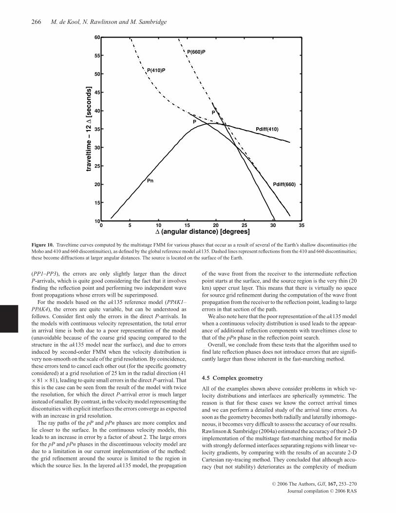
Figure 11. Ray paths representing late reflections from a highly deformed (‘egg carton’ shaped) interface. The reflection off the top of the interface bumproughly halfway between source and receiver is the shortest path, the other eight rays are late reflections.

increases, the errors were still comparable with those for simplecases with known solutions. This is consistent with our results, forexample, when comparing constant-velocity medium direct arrivalswith P-arrivals in the layered ak135 model. In the following, weexamine some results for fully 3-D problems.

As a first example, we calculate the ray paths for late reflec-tions from a highly deformed interface. The velocity is assumedto be constant and the resolution of the propagation grid is 51 ×101 × 101. In Fig. 11, a source and a receiver lie on the surface,exactly on the diagonal of the surface grid so that it is easier tounderstand the resulting ray paths. We are looking for phases thatare reflections from the strongly deformed interface below them,whose deformations (the product of two sine functions in latitudeand longitude) are also symmetric around the diagonal plane of thegrid. The shortest path, which is the path found when the standardmultistage fast-marching method is applied, is the reflection off thetop of the interface bump roughly halfway between source and re-ceiver. Because of the symmetry, five reflections lie exactly in thediagonal plane: two reflections off the bump below the source, oneoff the bump between source and receiver, and two off the bumpjust below the receiver. In addition, four ray paths are found that lieoutside the diagonal plane, and reflect off the sides of the interfacedeformations. The late reflections off the bump below the receiverand from the sides are likely to have higher amplitudes than the firstarrival.

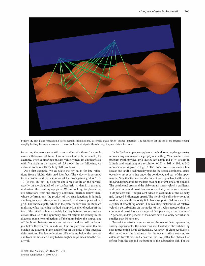
In the final example, we apply our method to a complex geometryrepresenting a more realistic geophysical setting. We consider a localproblem (with physical grid size 50 km depth and 1◦ ≈ 110 km inlatitude and longitude) at a resolution of 51 × 101 × 101. A 3-Drepresentation is given in Fig. 12. The model consists of a coast line(ocean and land), a sediment layer under the ocean, continental crust,oceanic crust subducting under the continent, and part of the uppermantle. Note that the water and sediment layers pinch out at the coastline and disappear under the land area on the right side of the image.The continental crust and the slab contain linear velocity gradients,and the continental crust has random velocity variations between+20 per cent and −20 per cent added to each node of the velocitygrid (spaced 4 kilometers apart). The tricubic B-spline interpolationused to evaluate the velocity field has a support of 64 nodes so thatsignificant smoothing occurs. The resulting distribution of relativevelocity perturbations on the nodes of the region representing thecontinental crust has an average of 3.6 per cent, a maximum of15 per cent, and 98 per cent of the nodes have a velocity perturbationsmaller than 10 per cent.

Two of the seismic sources are on the sea surface representingsurvey experiments, the other two are located in the subductingslab representing local earthquakes. An array of eight receivers isdistributed over the land area. For the ocean surface sources, wecalculate traveltimes and construct the ray paths for phases thatreflect from the top and the bottom of the subducting slab. For the

C© 2006 The Authors, GJI, 167, 253–270



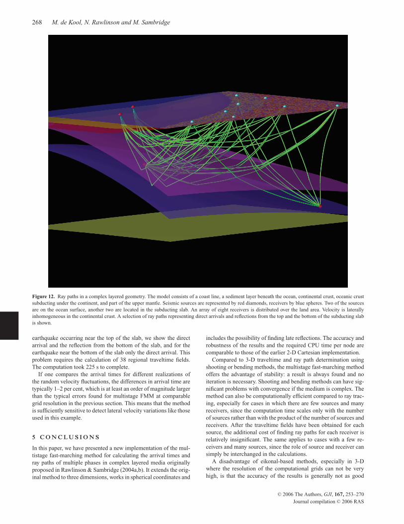
Figure 12. Ray paths in a complex layered geometry. The model consists of a coast line, a sediment layer beneath the ocean, continental crust, oceanic crustsubducting under the continent, and part of the upper mantle. Seismic sources are represented by red diamonds, receivers by blue spheres. Two of the sourcesare on the ocean surface, another two are located in the subducting slab. An array of eight receivers is distributed over the land area. Velocity is laterallyinhomogeneous in the continental crust. A selection of ray paths representing direct arrivals and reflections from the top and the bottom of the subducting slabis shown.

earthquake occurring near the top of the slab, we show the directarrival and the reflection from the bottom of the slab, and for theearthquake near the bottom of the slab only the direct arrival. Thisproblem requires the calculation of 38 regional traveltime fields.The computation took 225 s to complete.

If one compares the arrival times for different realizations ofthe random velocity fluctuations, the differences in arrival time aretypically 1–2 per cent, which is at least an order of magnitude largerthan the typical errors found for multistage FMM at comparablegrid resolution in the previous section. This means that the methodis sufficiently sensitive to detect lateral velocity variations like thoseused in this example.

5 C O N C L U S I O N S

In this paper, we have presented a new implementation of the mul-tistage fast-marching method for calculating the arrival times andray paths of multiple phases in complex layered media originallyproposed in Rawlinson & Sambridge (2004a,b). It extends the orig-inal method to three dimensions, works in spherical coordinates and

includes the possibility of finding late reflections. The accuracy androbustness of the results and the required CPU time per node arecomparable to those of the earlier 2-D Cartesian implementation.

Compared to 3-D traveltime and ray path determination usingshooting or bending methods, the multistage fast-marching methodoffers the advantage of stability: a result is always found and noiteration is necessary. Shooting and bending methods can have sig-nificant problems with convergence if the medium is complex. Themethod can also be computationally efficient compared to ray trac-ing, especially for cases in which there are few sources and manyreceivers, since the computation time scales only with the numberof sources rather than with the product of the number of sources andreceivers. After the traveltime fields have been obtained for eachsource, the additional cost of finding ray paths for each receiver isrelatively insignificant. The same applies to cases with a few re-ceivers and many sources, since the role of source and receiver cansimply be interchanged in the calculations.

A disadvantage of eikonal-based methods, especially in 3-Dwhere the resolution of the computational grids can not be veryhigh, is that the accuracy of the results is generally not as good

C© 2006 The Authors, GJI, 167, 253–270



as can be obtained with a properly converged iterative ray-tracingmethod. The accuracy that can be easily obtained with current com-putational resources (i.e. using grids with millions to tens of millionsof nodes) is, however, sufficient for many applications, including arange of 3-D tomographic imaging problems, for example, teleseis-mic tomography, wide-angle reflection/refraction tomography, localearthquake tomography and regional (continental scale) tomogra-phy. Because of the flexible parametrisation of the velocity fieldsand the interface positions in terms of nodal values on a grid andspline interpolation, it is in principle straightforward to treat thevelocities in each region and the position of each interface sepa-rately as either fixed or parameters to be inverted for. In the case ofteleseismic tomography, one could include interfaces that representcrustal structure that is constrained by other data; explicit repre-sentation of a dipping slab in local earthquake tomography may beadvantageous. The new scheme offers the possibility of combiningdifferent classes of data sets (e.g. local earthquake, refraction andteleseismic). The ability to include potentially complex interfaceand velocity structure, yet retain computational stability and effi-ciency makes the new scheme practical for large seismic imagingproblems.

We have shown that the multistage fast-marching method canprovide arrival times with relative errors between 0.1 and 0.01 percent for a range of synthetic examples, and that it performs robustlyfor very heterogeneous media approximating a realistic geophysicalsetting. Ultimately, the practicability of the method will be estab-lished by its application to real problems. The source code of ourimplementation is available for general use through a website athttp://rses.anu.edu.au/seismology/fmmcode/.

A C K N O W L E D G M E N T S

This work was supported by Australian Research Council DiscoveryProject DP0451133.

R E F E R E N C E S

Afnimar & Koketsu, K., 2000. Finite difference traveltime calculation forhead waves travelling along an irregular interface, Geophys. J. Int., 143,729–734.

Benamou, J.D., 1996. Big ray tracing: Multivalued traveltime field compu-tation using viscosity solutions of the Eikonal equation, J. Comp. Phys.,128, 463–474.

Bevc, D., 1997. Imaging complex structures with semirecursive Kirchhoffmigration, Geophysics, 62, 577–588.

Buske, S., 1999. 3-D prestack Kirchhoff migration of the ISO89-3D dataset, Pure appl. Geophys., 156, 157–171.

Cao, S. & Greenhalgh, S., 1994. Finite-difference solution of the eikonalequation using an efficient, first-arrival, wavefront tracking scheme, Geo-physics, 59, 632–643.

Cassell, B.R., 1982. A method for calculating synthetic seismograms inlaterally varying media, Geophys. J. R. astr. Soc., 69, 339–354.

Cheng, N. & House, L., 1996. Minimum traveltime calculations in 3-D graphtheory, Geophysics, 61, 1895–1898.

Chopp, D.L., 2001. Some improvements of the fast marching method, SIAMJ. Sci. Comput., 23, 230–244.

Day, A.J., Peirce, C. & Sinha, M.C., 2001. Three-dimensional crustal struc-ture and magma chamber geometry at the intermediate-spreading, back-arc Valu Fa Ridge, Lau Basin—results of a wide-angle seismic tomo-graphic inversion, Geophys. J. Int., 146, 31–52.

Fischer, R. & Lees, J.M., 1993. Shortest path ray tracing with sparse graphs,Geophysics, 58, 987–996.

Fomel, S. & Sethian, J.A., 2002. Fast-phase space computation of multiplearrivals, Proc. Nat. Acad. Sci., 99, 7329–7334.

Gray, S.H. & May, W.P., 1994. Kirchhoff migration using eikonal equa-tion traveltimes, Geophysics, 59, 810–817.

Hole, J.A., 1992. Nonlinear high-resolution three-dimensional travel-timetomography, J. geophys. Res., 97, 6553–6562.

Hole, J.A. & Zelt, B.C., 1995. 3-D finite-difference reflection travel times,Geophys. J. Int., 121, 427–434.

Julian, B.R. & Gubbins, D., 1977. Three-dimensional seismic ray tracing, J.Geophys., 43, 95–113.

Kennett, B.L.N., Engdahl, E.R. & Buland, R., 1995. Constraints on seis-mic velocities in the earth from traveltimes, Geophys. J. Int., 122, 108–124.

Kim, S. & Cook, R., 1999. 3-D traveltime computation using second-orderENO scheme, Geophysics, 64, 1867–1876.

Koketsu, K. & Sekine, S., 1998. Pseudo-bending method for three-dimensional seismic ray tracing in a spherical earth with discontinuities,Geophys. J. Int., 132, 339–346.

Lambare, G., Lucio, P.S. & Hanyga, A., 1996. Two-dimensional multival-ued traveltime and amplitude maps by uniform sampling of a ray field,Geophys. J. Int., 125, 584–598.

Moser, T.J., 1991. Shortest path calculation of seismic rays, Geophysics, 56,59–67.

Nakanishi, I. & Yamaguchi, K., 1986. A numerical experiment on nonlinearimage reconstruction from first-arrival times for two-dimensional islandarc structure, J. Phys. Earth, 34, 195–201.

Osher, S., Cheng, L.-T., Kang, M., Shim, H. & Tsai, Y.-H., 2002. Geometricoptics in a phase-space-based level set and Eulerian framework, J. Comp.Phys., 179, 622–648.

Podvin, P. & Lecomte, I., 1991. Finite difference computation of traveltimesin very contrasted velocity models: a massively parallel approach and itsassociated tools, Geophys. J. Int., 105, 271–284.

Popovici, A.M. & Sethian, J.A., 2002. 3-D imaging using higher order fastmarching traveltimes, Geophysics, 67, 604–609.

Qian, J. & Symes, W.W., 2002. An adaptive finite-difference method fortraveltimes and amplitudes, Geophysics, 67, 167–176.

Qin, F., Luo, Y., Olsen, K.B., Cai, W. & Schuster, G.T., 1992. Finite-difference solution of the eikonal equation along expanding wavefronts,Geophysics, 57, 478–487.

Rawlinson, N. & Sambridge, M., 2004a. Wavefront evolution in stronglyheterogeneous layered media using the Fast Marching Method, Geophys.J. Int., 156, 631–647.

Rawlinson, N. & Sambridge, M., 2004b. Multiple reflection and transmis-sion phases in complex layered media using a multistage fast marchingmethod, Geophysics, 69, 1338–1350.

Riahi, M.A. & Juhlin, C., 1994. 3-D interpretation of reflected arrival timesby finite-difference techniques, Geophysics, 59, 844–849.

Sambridge, M.S., 1990. Non-linear arrival time inversion: Constraining ve-locity anomalies by seeking smooth models in 3-D, Geophys. J. Int., 102,653–677.

Sethian, J.A., 1996. A fast marching level set method for monotonicallyadvancing fronts, Proc. Nat. Acad. Sci., 93, 1591–1595.

Sethian, J.A., 1999. Level Set Methods and Fast Marching Methods, Cam-bridge University Press, Cambridge.

Sethian, J.A. & Popovici, A.M., 1999. 3-D traveltime computation using thefast marching method, Geophysics, 64, 516–523.

Symes, W.W. & Qian, J., 2003. A slowness matching eulerian method formultivalued solutions of eikonal equaions, SIAM J. Sci. Comput., 19, 501–526.

Toomey, D.R., Solomon, S.C. & Purdy, G.M., 1994. Tomographic imagingof the shallow crustal structure of the East Pacific Rise at 9◦30′N, J.geophys. Res., 99, 24 135–24 157.

Um, J. & Thurber, C., 1987. A fast algorithm for two-point seismic raytracing, Bull. seism. Soc. Am., 77, 972–986.

van Trier, J. & Symes, W.W., 1991. Upwind finite-difference calculation oftraveltimes, Geophysics, 56, 812–821.

Vidale, J.E., 1988. Finite-difference calculations of traveltimes, Bull. seism.Soc. Am., 78, 2062–2076.

C© 2006 The Authors, GJI, 167, 253–270



Vidale, J.E., 1990. Finite-difference calculations of traveltimes in three di-mensions, Geophysics, 55, 521–526.

Vinje, V., Iversen, E. & Gjøystdal, H., 1993. Traveltime and amplitude esti-mation using wavefront construction, Geophysics, 58, 1157–1166.

Vinje, V., Åstebøl, K., Iversen, E. & Gjøystdal, H., 1999. 3-D ray modellingby wavefront construction in open models, Geophys. Prospect., 64, 1912–1919.

Xu, S. & Lambare, G., 2004. Fast migration/inversion with multivaluedrayfields: Part 1—Method, validation test, and application in 2-D to Mar-mousi, Geophysics, 69, 1311–1319.

Zelt, C.A. & Barton, P.J., 1998. Three-dimensional seismic refraction to-mography: A comparison of two methods applied to data from the FaeroeBasin, J. geophys. Res., 103, 7187–7210.

Zelt, B.C., Ellis, R.M., Zelt, C.A., Hyndman, R.D., Lowe, C., Spence, G.D.& Fisher, M.A., 2001. Three-dimensional crustal velocity structure be-neath the Strait of Georgia, British Columbia, Geophys. J. Int., 144, 695–712.

Zhao, P., Uren, N.F., Wenzel, F., Hatherly, P.J. & McDonald, J.A., 1998.Kirchhoff diffraction mapping in media with large velocity contrasts, Geo-physics, 63, 2072–2081.

C© 2006 The Authors, GJI, 167, 253–270


Documents

A practical grid-based method for tracking multiple ...rses.anu.edu.au/~malcolm/papers/pdf/dekool06.pdf · A practical grid-based method for tracking multiple refraction and reﬂection