Embed Size (px)
Citation preview

Preliminary Draft
A Pragmatist’s Guide to Long-run Equity Returns,
Market Valuation, and the CAPE
John Golob
Retired (Federal Reserve Bank of Kansas City)
5515 Crestwood Drive
Kansas City, MO 64110
(816)822-8463
Abstract
When practitioners evaluate the equity market, two important questions recur. What
long-run returns should investors expect? And, are there fundamental yardsticks that reliably
indicate when the market is overvalued? Researchers have not reached a consensus on either
of these questions. Equity prices have been high relative to their historical average, which has
led many analysts to predict future equity returns will be below their historical average.
Forecasts for real returns vary widely, however, from as low as 2%, to approximately 6%, which
is close to the 6.5% average since 1871. Disagreements about returns reflect disagreement
about how earnings will be affected by slower GDP growth, lower dividends, share buybacks,
and the profitability of retained earnings. The current paper introduces Federal Reserve Flow
of Funds and S&P500 book value data into this debate, and these data are generally supportive
of the optimistic forecasts for equity returns. Estimates of long-run returns have implications
for valuation metrics such as Shiller’s CAPE (cyclically adjusted price-earnings ratio).
December 2014
2
A Pragmatist’s Guide to Long-run Equity Returns, Market Valuation, and the CAPE
1. Introduction
When financial analysts, investment advisors, business journalists, and researchers
evaluate the equity market, two important questions recur. What long-run returns can
investors expect from equities?1 And, is there a reliable metric to determine when the market
is overvalued? Long-run equity returns are important both for investors saving for retirement
and for retirees who depend on equities for their living expenses. Lower returns require
workers to save more for retirement and require retirees to spend a lower percentage of their
accumulated financial assets. Higher returns allow the opposite, lower savings rates while
working and higher spending rates in retirement.
Both of the issues addressed in this paper, long-run equity returns and market valuation,
are ultimately linked to economic fundamentals. Equity returns depend on the growth rate of
corporate profits, which depend on growth rate of GDP. The relationship between valuation
and economic growth is more subtle, but higher growth rates generally support higher
valuations.
An example can illustrate the relationship between growth and valuation. Consider two
equities in the Dow Jones Average, Microsoft and United Health, which had the same $1.12
annual per-share dividend in early 2014. The price per share of United Health was almost
double that of Microsoft, because it was expected to grow faster than Microsoft. That is, the
present value of its expected future dividends was greater than Microsoft’s.2 The same logic
applies to the S&P 500 index. When the index is expected to grow faster, investors are willing
to pay a higher price for a dollar of current dividends. Stated in terms of the dividend yield,
investors will accept a lower dividend yield when they expect the index to grow faster. Again,
valuation depends on growth.
1 Long-run equity returns are often discussed in the context of the equity premium, which is the difference
between equity returns and Treasury interest rates. This more difficult question is addressed extensively in (Hammond, Leibowitz, and Siegel, eds. 2011) 2 On January 28, 2014 the closing price of Microsoft was 36.27 versus 71.71 for United Health. In the Argus Analyst
Reports from January 2014, the expected 5-yr growth rate is 8% for Microsoft and 15% for United Health.
3
The current paper analyzes the prospects for long-run equity returns by focusing on per
share earnings growth for the S&P 500 index.3 Actual returns are calculated by adding
dividends to price changes, but these components of return are not as closely connected to
economic fundamentals as earnings. Dividends can change with payout policy, and prices can
change with investor sentiment. Over the long-run, however, both dividends and prices follow
corporate earnings. And if prices and dividends grow at the same rate as earnings, the long-run
return is just the dividend yield plus the growth rate.
Another rationale for focusing on earnings is that disagreements among analysts and
researchers regarding long-run returns are largely a result of different forecasts for earnings
growth. So, resolving the debate about earnings helps resolve the debate about returns.
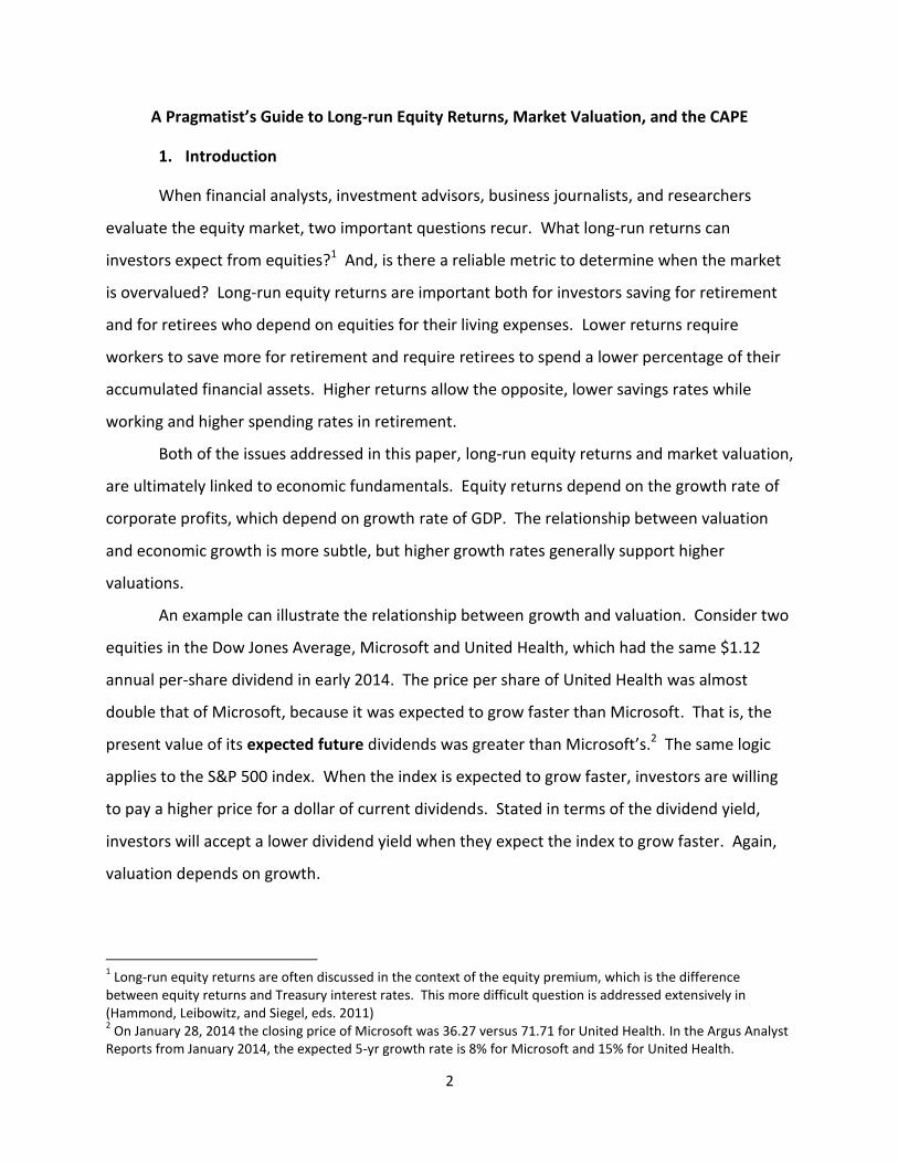
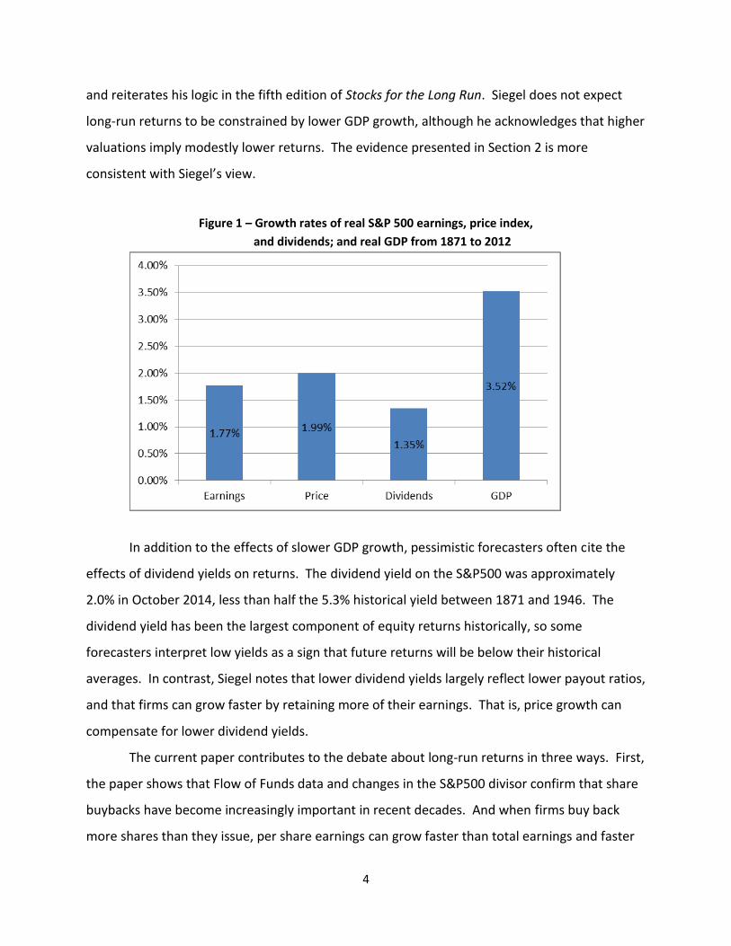
As background for a discussion about long-run earnings growth, Figure 1 illustrates the
real growth rates of S&P 500 earnings, prices, and dividends between 1871 and 2012; and the
growth rate of real GDP over this same period.4 The financial variables are inflation-adjusted
with the CPI. The figure shows similar long-run growth rates for the price index (1.99%) and
earnings (1.77%). Equity prices rose a little faster than earnings, reflecting an increase in the
price-earnings multiple between 1871 and 2012. Dividends grew more slowly (1.35%) because
the fraction of earnings paid as dividends, the payout ratio, dropped from about 65% in 1871 to
36% in 2012. Note that real prices and earnings have grown much more slowly than the 8.7%
annual nominal return over this period, which includes dividends and inflation.
The final item in the figure is real GDP, which grew 3.52% per year on average. This is
over double the growth rate of dividends and substantially higher than the growth rates for
either prices or earnings. Because the S&P 500 has grown more slowly than GDP in the past,
some market observers have argued that the S&P 500 should grow more slowly than GDP in the
future (Gross, 2012; Arnott, 2010). Siegel (2014:162) is on the optimistic side of this debate,
3 Researchers generally use the S&P 500 index to analyze the equity market because the data extend back to the
19th
century, and because its capitalization weighting more accurately reflects the economic importance of each component. The index was expanded to include 500 stocks in 1957. This paper uses data downloaded from Professor Robert Shiller’s website: http://aida.wss.yale.edu/~shiller/data.htm. 4 Annual GDP data back to 1929 are from the National Income and Product Accounts, available at
http://www.bea.gov/scb/index.htm#chartsandtables. Economic output between 1871 and 1929 are from the NBER at http://www.nber.org/data/abc/. Annual averages throughout this paper are calculated geometrically rather than arithmetically.
4
and reiterates his logic in the fifth edition of Stocks for the Long Run. Siegel does not expect
long-run returns to be constrained by lower GDP growth, although he acknowledges that higher
valuations imply modestly lower returns. The evidence presented in Section 2 is more
consistent with Siegel’s view.
Figure 1 – Growth rates of real S&P 500 earnings, price index,
and dividends; and real GDP from 1871 to 2012
In addition to the effects of slower GDP growth, pessimistic forecasters often cite the
effects of dividend yields on returns. The dividend yield on the S&P500 was approximately
2.0% in October 2014, less than half the 5.3% historical yield between 1871 and 1946. The
dividend yield has been the largest component of equity returns historically, so some
forecasters interpret low yields as a sign that future returns will be below their historical
averages. In contrast, Siegel notes that lower dividend yields largely reflect lower payout ratios,
and that firms can grow faster by retaining more of their earnings. That is, price growth can
compensate for lower dividend yields.
The current paper contributes to the debate about long-run returns in three ways. First,
the paper shows that Flow of Funds data and changes in the S&P500 divisor confirm that share
buybacks have become increasingly important in recent decades. And when firms buy back
more shares than they issue, per share earnings can grow faster than total earnings and faster
5
than GDP. This refutes the pessimistic assertion that per share earnings growth will be
constrained by GDP growth.
The second contribution of the paper is to look at the trends in corporate profitability
using both Flow of Funds data and S&P500 earnings and net worth data. Pessimistic views of
future returns implicitly assume that firms will become less profitable, but neither data source
shows any substantial decline in the ratio of firms’ income to book value.
The third contribution of the paper is to examine Siegel’s (2014:147) assertion that
returns are unaffected by the payout ratio. His logic assumes that the return firms earn on
retained earnings is identical to the return investors require to hold equities. Section 2
examines the implications of relaxing this assumption. Over the last four decades S&P500 firms
have earned more on their retained earnings than the historical equity return. Under these
conditions, reducing the payout ratio raises the long-run return.
The remainder of the paper is organized as follows. Section 2 analyzes the economic
forces that determine long-run earnings growth, and discusses the implications for long-run
equity returns. Trends in share buybacks and firm profitability are examined with S&P500 and
Federal Reserve Flow of Funds data. The section also explores how returns vary with the
payout ratio when the return firms earn on retained earnings exceeds the equity return to
shareholders. Section 3 considers the implications of the results from Section 2 on equity
valuations and Shiller’s CAPE (cyclically adjusted price-earnings). Section 4 concludes.
2. Long-Run Equity Returns
The first question to address regarding long-run returns is: what time horizon is long-
run? This paper will not focus on a precise time horizon, but rather, will consider the long-run
as the time it takes for economic fundamentals to become more important for returns than
short-term movements in investor sentiment or the booms and busts of the business cycle.
While the relationship between stock prices, earnings, and GDP can vary widely for periods
exceeding a decade, stock prices ultimately follow earnings, which are a relatively stable
fraction of GDP. As evidence of the importance of economic fundamentals over long horizons,
6
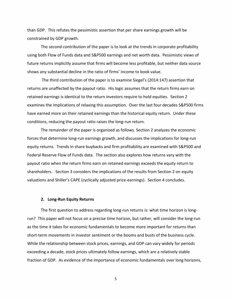
researchers find that equity returns have been more predictable over ten to thirty year
horizons than over shorter ones (Campbell and Shiller, 1987).
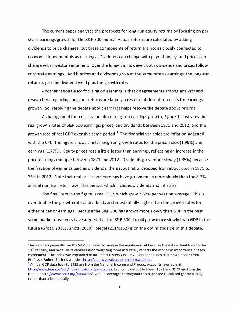
Figure 2 - Real earnings on S&P500 index
As a note of caution about long-run forecasts, although earnings on the S&P index have
risen substantially over the last 140 years, they have been very volatile, and even stagnated for
one lengthy period. Figure 2 shows real S&P500 earnings and the 10-year average, which is the
metric favored by Shiller (2000). The ten-year average trended down from 1917 (when the U.S.
entered WWI) to 1939. Real earnings in 1948 were about the same as in 1907 (both years were
business cycle peaks), so the return to equities during this period was approximately equal to
the dividend yield, about 5%. The lack of earnings growth over the 41-year period that included
two world wars and the Great Depression illustrates a peril of long-run forecasts. If the next 40
years encompass two world wars and another depression, a forecast based on benign economic
and political conditions will likely be far off target. And of course, if the U.S. loses a world war
the outlook for S&P500 returns will be even bleaker.
Having offered the appropriate caveat about forecasting, I now consider alternative
opinions about future equity returns. Most of the disagreement about future returns can be
traced to disagreements about how two economic forces will affect returns, lower dividend
yields and slower GDP growth. The dividend yield on the S&P500 as of the current writing is
2.0%, which is less than half the 4.4% average dividend yield between 1871 and 2012. The
7
current consensus forecast for 10-year real GDP growth is 2.6% (Livingston Survey, 2013), which
is almost a percent lower than the 3.52% average between 1871 and 2012.
Considering first some pessimistic return forecasts, Gross (2012) suggests that the
current economic environment implies future nominal equity returns of 4%, which implies real
returns of only 2%.5 Bernstein and Arnott (2003) contend that per share earnings must grow
more slowly than GDP. When corporations issue additional shares, their earnings get diluted,
so per share earnings grow more slowly than total earnings. Historically, dilution has averaged
about 2 percent per year in the U.S. (the difference between column 1 and column 4 in Figure
1), and Bernstein-Arnott treat this empirical observation as a law of nature, noting that “new
share issuance in many nations almost always exceeded stock buybacks by an average of 2
percent or more per year.” Following this logic, 2.5% GDP growth would imply per share
earnings growth of only 0.5%. Adding this growth rate to a 2% dividend yield implies a real
return of 2.5%.6 These two forecasts, of real returns around 2.0-2.5%, are representative of the
pessimistic view.
Siegel (2014: 162) is on the optimistic side of the long-run return debate. Siegel
contends that the best estimate of long-run returns is the earnings yield. He notes that the
6.7% average earnings yield is very close to the 6.6% average return over the period from 1802
to 2012. To understand this result, consider the case when 100% of earnings are paid as
dividends, so the net worth (and price) of the firm doesn’t change. In this case the dividend
yield is the same as the earnings yield, which is the total return. If instead, earnings are
reinvested, the value of the business and the price of the equity will grow enough to
compensate for the lower dividend yield.7 Using March 2014 estimates of forward S&P500
earnings, Siegel’s strategy forecasts a real return of about 6%.8
5 The Federal Reserve’s inflation target is 2% (Federal Reserve System, 2012). As of March 2014, the S&P500 has
risen about 30% since Gross’ August 2012 forecast. Applying his logic after this subsequent rise could lead to an even more pessimistic forecast. 6 In a more recent article, Arnott (2011) suggests future equity returns in the range of 2.5-3.0%.
7 In theory, returns will be totally independent of dividend policy when the return-on-equity of the reinvested
dividends is the same as the return required by equity investors. 8 The S&P500 earnings forecast for 2014 was downloaded the S&P website:
http://us.spindices.com/indices/equity/sp-500. The S&P500 divisor was also downloaded from this site.
8
Since buybacks are an important source of the disparity in long-run return forecasts, the
following discussion examines trends in share issuance and buybacks.
Share issuance versus buybacks
When analysts assert that S&P500 per share earnings cannot grow faster than GDP, they
are making an implicit assumption about the importance of share buybacks. When a company
buys back its publicly traded shares, their per-share earnings grow faster than total earnings.
This same logic applies to an aggregate index, if S&P500 companies are aggregate buyers of
their own shares, per-share earnings of the index will grow faster than total earnings. Under
this condition, per share earnings can grow faster than GDP. Historically, corporations have
been net issuers of shares, such that per-share earnings have grown slower than GDP. Thus, a
crucial question is: Can corporations become net buyers rather than net issuers of shares? Two
different data sources suggest they are already net buyers.
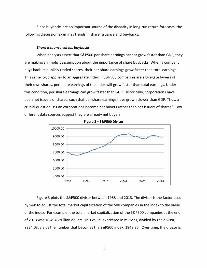
Figure 3 – S&P500 Divisor
Figure 3 plots the S&P500 divisor between 1988 and 2013. The divisor is the factor used
by S&P to adjust the total market capitalization of the 500 companies in the index to the value
of the index. For example, the total market capitalization of the S&P500 companies at the end
of 2013 was 16.4948 trillion dollars. This value, expressed in millions, divided by the divisor,
8924.03, yields the number that becomes the S&P500 index, 1848.36. Over time, the divisor is

9
adjusted for share issuance and buybacks, share issuance raises the divisor and share buybacks
lower the divisor.
The figure shows the divisor mostly rising until 2004:Q3. Between 1990:Q4 and
2004:Q3, the divisor rose by about 40%, corresponding to a 2.5% annual rate, which is
comparable to the long-term historic average noted by Bernstein and Arnott (2003). Between
2004:Q3 and 2013:Q3, however, the divisor fell by 4.6%, corresponding to a 0.5% average
decline per year. This implies that S&P500 per-share earnings would rise 0.5% per year faster
than total earnings during this period.
The Federal Reserve Flow of Funds accounts provide a broader measure of share
issuance and buybacks by U.S. corporations than the S&P500 divisor. Figure 4 plots the Flow of
Funds data between 1947 and 2013.9 The plot is almost always positive until 1984, indicating
net issuance, but alternates between net issuance and net buyback afterwards. The post-1984
surge in buybacks had two causes. First, leveraged buyouts increased as investment bankers
developed junk bonds as a new source of financing. Second, the Securities and Exchange
Commission passed Rule 10b-18, which reduced restrictions on companies buying back their
own shares.
Figure 4 – Share Issuance/Buybacks from Flow of Funds
9 The plot in the chart is calculated as the ratio of line 1 of Table F.213, net issues of corporate equities, over line 1
of Table L.213, market value of corporate equities. The market value of equities within the quarter is assumed to be the average of the values at the beginning and end of the quarter.
10
The average share issuance from Figure 4 is 0.75% per year pre-1984, but -0.5% per year
afterwards, indicating net buybacks. These averages apply to all U.S. corporations, not just the
S&P500, but the switch from issuance to buybacks helps explain why S&P500 earnings grew
faster in the later period. Even though real GDP grew more slowly after 1984 (2.8%) than
before (3.6%), real S&P500 earnings grew faster after 1984 (2.4%) than before (2.1%). That is,
slower GDP growth did not lead to slower per share earnings growth.
To sum up this section on share issuance and buybacks, changes in the S&P divisor show
net share buybacks over the last decade. Flow of Funds data show net buybacks since 1984.
These buybacks are not consistent with analysts’ assertions that per share earnings must grow
slower than GDP. Issuance and buyback policies have varied widely in historical data, so it is
difficult to project what will happen in the future. Nevertheless, if buybacks continue, per
share earnings growth need not be constrained by GDP growth.
Profitability of retained earnings
A second component of analysts’ disagreement about future equity returns is their view
about the profitability of retained earnings. Retained earnings have risen, but these retentions
must be invested profitably if they are to contribute to future earnings growth and future
equity returns. Arnott and Asness (2003) offer a very pessimistic outlook on this issue, and
present evidence that higher retained earnings lead to lower rather than higher earnings
growth. Their counterintuitive result is discussed further in the Appendix. Bernstein (2013)
also makes a case for lower profitability, concluding: “As technology makes the world ever
wealthier, the returns on both riskless and risky assets will of necessity fall.”
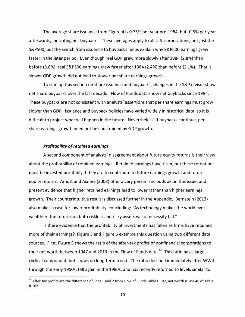
Is there evidence that the profitability of investments has fallen as firms have retained
more of their earnings? Figure 5 and Figure 6 examine this question using two different data
sources. First, Figure 5 shows the ratio of the after-tax profits of nonfinancial corporations to
their net worth between 1947 and 2013 in the Flow of Funds data.10 This ratio has a large
cyclical component, but shows no long-term trend. The ratio declined immediately after WWII
through the early 1950s, fell again in the 1980s, and has recently returned to levels similar to
10
After-tax profits are the difference of lines 1 and 2 from Flow of Funds Table F.102, net worth is line 46 of Table B.102.
11
those in the 1950s. Thus, although retained earnings have trended upwards over the last 50
years, Flow of Funds data offer no evidence that firms have been unable to invest these
retentions profitably.
Figure 5 – Flow of Funds measure of firm profitability
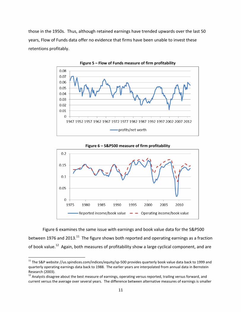
Figure 6 – S&P500 measure of firm profitability
Figure 6 examines the same issue with earnings and book value data for the S&P500
between 1976 and 2013.11 The figure shows both reported and operating earnings as a fraction
of book value.12 Again, both measures of profitability show a large cyclical component, and are
11
The S&P website //us.spindices.com/indices/equity/sp-500 provides quarterly book value data back to 1999 and quarterly operating earnings data back to 1988. The earlier years are interpolated from annual data in Bernstein Research (2003). 12
Analysts disagree about the best measure of earnings, operating versus reported, trailing versus forward, and current versus the average over several years. The difference between alternative measures of earnings is smaller
12
lower in the recent expansion than in the late 1990s. Nevertheless, both metrics are higher
now than through most of the 1980s, and show no long-term downtrend. To sum up, neither
Flow of Funds nor S&P500 data are consistent with the pessimists’ view that firms are
becoming less profitable.
Return-on-book value versus investors required return
Thus far, evidence on share buybacks and corporate profitability support Siegel’s
optimistic outlook for equity returns. However, his assertion that returns are independent of
firms’ payout policy depends on an important assumption: that the return firms earn on their
retained earnings is equal to the return investors require to hold equities. Under this
assumption, the return to investors is equal to the earnings yield. The following discussion
considers the situation where these three returns are not equal. An equation for the return to
investors is developed for the case when firms’ internal return differs from the earnings yield.
Under market conditions over the last four decades, the analysis reveals that lower payout
ratios should raise the return to equities.
The ratio of income to book value in Figure 6 indicates how profitably S&P500 firms
invest their retained earnings. Most financial analysts refer to this ratio as the return-on-
equity (ROE). But to avoid confusion in the following discussion, where equity refers to share
ownership, the ratio will be labeled return-on-book value (RBV). The average RBV on S&P500
reported earnings was 13% between 1976 and 2013, which is almost double the 6.7% average
earnings yield. The algebra below shows how this divergence affects the return to investors.
To avoid unnecessary complications, the following derivation will consider the situation
where no shares are issued or bought back, so earnings are either retained or paid as dividends.
First, the return (R) is defined as the sum of price growth (G) and the dividend yield, which is
the ratio of dividend over price (D/P).
𝑅 = 𝐺 + 𝐷/𝑃
In the long-run, if RBV, the payout ratio, and the P/E ratio don’t change; prices and earnings will
grow at the same rate as book value. And the percentage change in book value is the ratio of
reinvested earnings to book value (BV). Making some substitutions, reinvested earnings equal
than the variability of long-run returns, so the current paper will not enter this debate. See Siegel (2014: 150-156) for an excellent discussion of S&P operating versus reported earnings.
13
total earnings (E) multiplied by one minus the payout ratio (PO), and dividends equal earnings
times the payout ratio, yields the following:
𝑅 = (1 − 𝑃𝑂) × 𝐸
𝐵𝑉+ 𝑃𝑂 ×
𝐸
𝑃 = (1 − 𝑃𝑂) × 𝑅𝐵𝑉 + 𝑃𝑂 ×
𝐸
𝑃
This equation has a straightforward interpretation. The total return is a weighted average of
the RBV and the earnings yield, where the weight is the payout ratio. The intuition is as follows:
an investor gets the earnings yield on the part received as dividends, but gets the RBV on the
part retained. Note that RBV and the earnings yield both have earnings in the numerator, only
the denominator differs. And when equity prices are above book value, as they have for most
of the last four decades, RBV will be greater than the earnings yield. Under these conditions,
reducing the payout ratio raises the return on equities. As a final observation about the
equation, when RBV equals the earnings yield, the return is also equal to the earnings yield, per
Siegel (2014:147).
The algebra can be extended to allow share buybacks, but the equation is not suitable
for the real world situation where buybacks are cyclical. The effect of buybacks on returns
depends on equity prices at the time of the buyback, and using an average value is not realistic.
Over the past decade firms have tended to buy back shares when cash flow, earnings, and
share prices were high, and then issued shares when cash flow, earnings, and prices were low.
This buy high/sell low behavior implies that share buybacks are less effective in raising the
growth of net worth than implied by calculations with long-run averages. With this caveat,
extending the above algebra to include share buybacks leads to an expression that is
approximately another weighted average, where the weights are the fractions of earnings
retained, paid as dividends, and shares bought back. An investor gets the earnings yield on the
fraction paid as dividends, approximately the earnings yield on the fraction used to buy back
shares, and approximately the RBV on the fraction reinvested. The reason for describing this
more complicated expression is to note that the presence of buybacks does not change the
positive effect of lower payout ratios on equity returns when RBV is above the earnings yield.
Nevertheless, quantifying the overall impact of share issuance and buybacks is complicated by
their cyclical behavior and is beyond the scope of the current paper.
14
To sum up this entire section, the shift from net share issuance to net buybacks implies
that per share earnings can grow faster rather than slower than GDP. Moreover, neither
S&P500 nor Flow of Funds data show any decline in firm profitability, and if firms continue to
make profitable investments shareholders can receive these profits as dividends or increases in
share value. Finally, accounting algebra implies that when RBV is greater than the earnings
yield, increasing the share of earnings reinvested should raise long-run returns. All of these are
consistent with the optimistic forecasts for returns. Unfortunately, cyclical variations in share
buybacks and issuance make it difficult to quantify their effect on returns.
3. Market Valuation and the CAPE
The above discussion about long-run returns has implications for equity valuation.
Researchers have found a relationship between equity valuations future returns (Fama and
French, 1987, Campbell and Shiller, 1988), so some financial advisors use valuation metrics to
adjust the fraction of investor assets allocated to equities. Two common metrics are the P/E
ratio and the CAPE.13 But, a shift in the composition of returns from dividends to growth has
implications for the equilibrium level of the CAPE. Valuation metrics can also be affected by
changes in the risk-free rate.
Shiller’s CAPE
Shiller (2000) proposed a modification of the P/E ratio, known as CAPE (cyclically
adjusted P/E), that is widely cited in the financial press, and has even been applied to
international equity markets (Badkar, 2014). CAPE is the ratio of the current price on the
S&P500 to a ten-year average of real S&P500 earnings (nominal earnings deflated by the CPI).
The rationale for CAPE is that earnings are highly cyclical, so earnings at the peak of the cycle
are not sustainable, and a P/E calculated with peak-cycle earnings is too optimistic. Similarly, a
P/E calculated with recessionary earnings is too pessimistic. As of early October 2014, with the
S&P500 near 1960, Shiller’s CAPE is 25.7, over 50% above its 16.5 historical mean.14
13
Fama and French (1987) find that the dividend yield has predictive power in historical data. But with changes in payout policies in recent decades, the relevance of their result for current forecasts is suspect. 14
A calculation of CAPE is updated every 10 minutes at: http://www.gurufocus.com/shiller-PE.php.
15
Siegel (2013) asserts that Shiller’s CAPE is too pessimistic because of changes in the
growth rate of per-share earnings. When earnings grow faster, the CAPE measure of past
earnings is lower relative to future earnings, which drives the CAPE higher (lower denominator).
The following example illustrates the effect. Consider two cases where the P/E is 15 (earnings
yield is 6.67%), but have different return components. In the first case, a 6.67% return consists
of a 5% dividend yield and 1.67% earnings growth (averages similar to those between 1871 and
1971). In the second case, a 6.67% return consists of 2% dividend yield and 4.67% earnings
growth. The CAPE equals 16.16 in the first case, and 24.19 in the second case.15 Thus, although
both of these cases have identical P/E ratios, and would provide investors the same expected
return absent changes in the P/E ratio, the CAPE is almost 50% higher in the second case.
Again, the CAPE is not a robust metric of future returns when the composition of returns shifts
from dividends to growth.
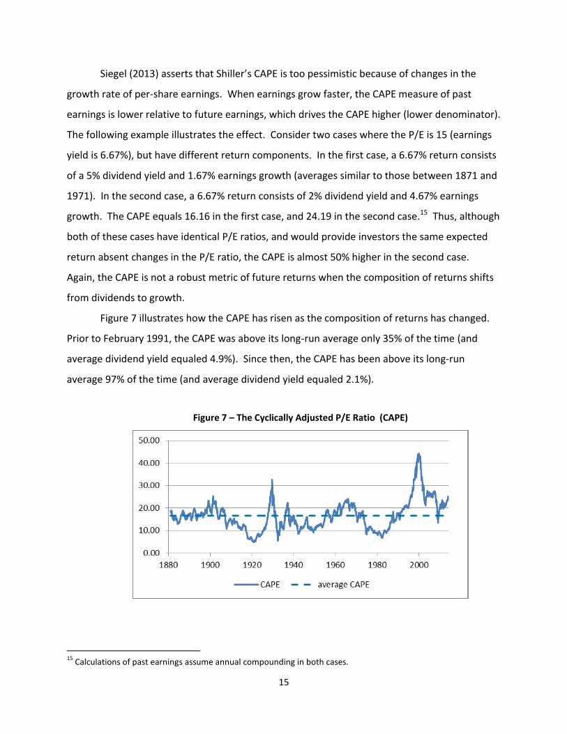
Figure 7 illustrates how the CAPE has risen as the composition of returns has changed.
Prior to February 1991, the CAPE was above its long-run average only 35% of the time (and
average dividend yield equaled 4.9%). Since then, the CAPE has been above its long-run
average 97% of the time (and average dividend yield equaled 2.1%).
Figure 7 – The Cyclically Adjusted P/E Ratio (CAPE)
15
Calculations of past earnings assume annual compounding in both cases.
16
The risk-free rate
Changes in interest rates can also interfere with efforts to determine when the market is
over-valued or under-valued. Analysts often divide the return investors expect from equities
into two components, a risk-free rate plus the equity premium. The equity premium is the
difference between the return investors expect from equities and the return on risk-free
securities. If the equity premium is stable, a lower risk-free rate implies investors will also
accept a lower return on risky securities. One measure of the risk-free rate is the interest rate
on short-term Treasury bills, which declined from 3.1% on average between 1871 and 1925, to
only 0.6% between 1925 and 2012 (Siegel, 2014:85). And if investors also accept a lower return
on risky securities, equity valuations should rise. This implies that valuation metrics based on
140-year averages will not pertain to the current environment.
Interest rates on inflation protected securities (TIPS) also support the view that real
interest rates have fallen. Economists often interpret the rate on TIPS as a measure of real
interest rates. Over five years into the latest economic recovery TIPS interest rates remain
between one and two percent lower than in the early 2000s.16 And if these lower risk-free
rates imply that investors will also accept lower returns on equities, equity valuations should be
above their historical averages. Kocherlakota (2013) offers reasons for the low interest rate
environment, and suggests low rates could persist for five to ten years.
To sum up this section, determining when the equity market is overvalued or
undervalued is not an easy task. The CAPE, a widely cited metric, could be affected by changes
in the growth rate of earnings. The equilibrium P/E and CAPE could also be affected by changes
in the risk-free rate. Both of these changes could push the CAPE higher, but it is difficult to say
how much higher.
4. Conclusion
This paper began by asking two questions. First, what long return should investors
expect from equities? Some analysts have argued that real returns will be substantially below
their 6.5% historical average because GDP growth has slowed and dividend yields have
16
Current rates on TIPS can be found in the online Wall Street Journal: http://online.wsj.com/mdc/public/page/2_3020-tips.html
17
declined. But, the evidence in Section 2 shows that returns are not necessarily constrained by
GDP growth. As GDP growth has slowed, firms have switched from net share issuance to net
buybacks, implying that per share earnings can grow faster than GDP. And dividend yields are
mostly lower because firms are reinvesting more of their earnings, so that their earnings should
grow faster. Moreover, pessimistic forecasts of equity returns presume that firms will become
less profitable, but neither Flow of Funds nor S&P500 book value data reveal any substantial
decline in profitability. Finally, the ratio of earnings-to-book value on the S&P500 exceeds its
earnings yield, which implies that a lower payout ratio will raise long-run returns. On balance,
there is no compelling evidence that equity returns will be substantially below their historical
average. An important caveat to this discussion, of course, is that returns can vary widely for
extended periods. For example, the real return on the S&P500 averaged about 15% during the
1990s, but minus 3% the following decade.
The second question, about market valuation, is more problematic. The CAPE has
recently been about 50% above its historical average, but the paper discusses two reasons why
this may not signal market overvaluation. Even if long-run returns are stable, the CAPE will rise
when the composition of returns shifts from dividends to growth. Also, if the equity premium
remains stable as interest rates decline, both the equilibrium P/E and CAPE of the market
should rise above their historical average. The instability of these metrics may explain why
Malkiel (2004) was unable to develop a successful trading strategy with the CAPE or other
valuation models. Although high profits and high P/E ratios near business cycle peaks are
tempting to those seeking an effective trading strategy, these business cycle peaks are more
apparent in hindsight than foresight.
18
References
Arnott, Robert. 2010. “Lessons from the ‘Naughties.’” Research Affiliates Fundamentals,
February.
http://www.researchaffiliates.com/Our%20Ideas/Insights/Fundamentals/Pages/F_2010_Feb_L
essons_From_the_Naughties.aspx.
Arnott, Robert. 2011. “Equity Risk Premium Myths.” in Rethinking the Equity Premium. P. Brett
Hammond, Jr., Martin L. Leibowitz, and Laurence B. Siegel, eds. Charlottesville, VA: CFA
Institute.
Arnott, Robert D. and Clifford S. Asness. 2003. “Surprise! Higher Dividends = Higher Earnings
Growth.” Financial Analysts Journal, January/February, 70-87.
Arnott, Robert. D and Peter L. Bernstein. 2002. “What Risk Premium is ‘Normal’?” Financial
Analysts Journal, March/April, 64-85.
Badkar, Mamta. 2014. “This Could be the Time to Invest in Russian Stocks.” Business Insider
Australia, (March 5, 2014).
http://www.businessinsider.com.au/russian-stocks-appear-oversold-and-cheap-2014-3.
Bernstein, William J. 2013. “The Paradox of Wealth.” Financial Analysts Journal,
September/October, 18-25.
Bernstein, William J. and Robert D. Arnott. 2003. “Earnings Growth: The Two Percent Dilution.”
Financial Analysts Journal, September/October, 47-55.
Bernstein Research. 2003. Bernstein Disciplined-Strategies Monitor, December, 63.
Campbell, John Y. and Robert J. Shiller. 1988. “Stock Prices, Earnings, and Expected Dividends.”
Journal of Finance, Vol. 43. No. 3, 661-676.
Fama, Eugene F. and Kenneth R. French. 1987. “Dividend Yields and Expected Stock Returns.”
Journal of Financial Economics 22, 3-25.
Federal Reserve System. 2012. FOMC Press Release on Monetary Deliberations, January 25.
http://www.federalreserve.gov/newsevents/press/monetary/20120125c.htm
19
Gross, Bill. 2012. “Cult Figures.” PIMCO Investment Outlook, August.
http://pimco.com/en/insights/pages/cult-figures.aspx
Hammond, Brett P., Martin L. Leibowitz, and Laurence B. Siegel, eds. 2011. Rethinking the
Equity Premium, Charlottesville, VA: CFA Institute.
Kocherlakota, Narayana. 2013. “Low Real Interest Rates.” Speech delivered at the 22nd Annual
Hyman P. Minsky Conference, Levy Economics Institute of Bard College, Annandale-on-Hudson,
N.Y., April 18,
http://www.minneapolisfed.org/news_events/pres/kocherlakota_speech_04-18-13.pdf
Livingston Survey. 2013. Federal Reserve Bank of Philadelphia, December 12.
Malkiel, Burton G. 2003. “Models of Stock Market Predictability.” The Journal of Financial
Research, Vol. 27:4, Winter, 449-459.
Ritter, Jay R. 2012. “Is Economic Growth Good for Investors?” Journal of Applied Corporate
Finance, Vol. 24, No. 3, 8-19
Shiller, Robert J. 2000. Irrational Exuberance. Princeton: Princeton University Press.
Siegel, Jeremy J. 2000. “Big Cap Tech Stocks Are a Sucker’s Bet.” Wall Street Journal, March 14,
A8.
Siegel, Jeremy J. 2011. “Long-Term Stock Returns Unshaken by Bear Markets.” in Rethinking the
Equity Premium, Hammond, Brett P., Martin L. Leibowitz, and Laurence B. Siegel, eds.
Charlottesville, VA: CFA Institute.
Siegel, Jeremy J. 2013. “The Shiller CAPE Ratio: A New Look.” Working Paper, The Wharton
School, May.
Siegel, Jeremy J. 2014. Stocks for the Long Run. Fifth Edition, New-York: McGraw-Hill.
20
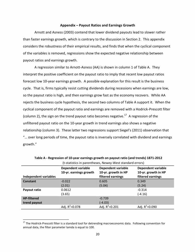
Appendix – Payout Ratios and Earnings Growth
Arnott and Asness (2003) contend that lower dividend payouts lead to slower rather
than faster earnings growth, which is contrary to the discussion in Section 2. This appendix
considers the robustness of their empirical results, and finds that when the cyclical component
of the variables is removed, regressions show the expected negative relationship between
payout ratios and earnings growth.
A regression similar to Arnott-Asness (AA) is shown in column 1 of Table A. They
interpret the positive coefficient on the payout ratio to imply that recent low payout ratios
forecast low 10-year earnings growth. A possible explanation for this result is the business
cycle. That is, firms typically resist cutting dividends during recessions when earnings are low,
so the payout ratio is high, and then earnings grow fast as the economy recovers. While AA
rejects the business cycle hypothesis, the second two columns of Table A support it. When the
cyclical component of the payout ratio and earnings are removed with a Hodrick-Prescott filter
(column 2), the sign on the trend payout ratio becomes negative.17 A regression of the
unfiltered payout ratio on the 10-year growth in trend earnings also shows a negative
relationship (column 3). These latter two regressions support Siegel’s (2011) observation that
“… over long periods of time, the payout ratio is inversely correlated with dividend and earnings
growth.”
Table A - Regression of 10-year earnings growth on payout ratio (and trends) 1871-2012
(t-statistics in parentheses, Newey-West standard errors)
Independent variables
Dependent variable 10-yr. earnings growth
Dependent variable 10-yr. growth in HP filtered earnings
Dependent variable 10-yr. growth in HP filtered earnings
Constant -0.022 (2.01)
0.605 (5.04)
0.349 (5.24)
Payout ratio 0.0612 (3.65)
-0.314 (-4.16)
HP-filtered trend payout
-0.739 (-4.03)
Adj. R2=0.078 Adj. R2=0.201 Adj. R2=0.090
17
The Hodrick-Prescott filter is a standard tool for detrending macroeconomic data. Following convention for annual data, the filter parameter lamda is equal to 100.