Embed Size (px)
Citation preview

1
eAppendix
A. Preliminary analyses: simulation study
To detect whether the statistic approach that corrects for serial correlation was necessary and did not
reduce the probability of detecting a statistically significant association, we conducted a simulation
analysis.
Simulated data. We relied on simulated data to assess our methods. Using the arima.sim function in R,
we first simulated two independent time series with auto-regression components:
𝑥1(𝑡) = 𝜑𝑥,1𝑥1(𝑡 − 1) + 𝜑𝑥,2𝑥1(𝑡 − 2) + ⋯ + 𝜑𝑥,𝑚𝑥1(𝑡 − 𝑚) + 휀(𝑡)
𝑦(𝑡) = 𝜑𝑦,1𝑦(𝑡 − 1) + 𝜑𝑦,2𝑦(𝑡 − 2) + ⋯ + 𝜑𝑦,𝑛𝑦(𝑡 − 𝑛) + 휀(𝑡),
where the errors are assumed to be independent and identically distributed according to the standard
normal distribution, 휀(𝑡)~𝒩(0,1).
The number of auto-regression terms in each equation, m and n, was randomly selected from a Poisson
distribution with mean 3.
Then, we generated two time series 𝑥2(𝑡) and 𝑥3(𝑡) that were associated with 𝑦(𝑡):
𝑥2(𝑡) = 𝑥1(𝑡) + 𝒩(1.5,1, 𝑡)𝑦(𝑡) + 휀(𝑡)
𝑥3(𝑡) = 𝒩(1.5,1, 𝑡)𝑦(𝑡) + 휀(𝑡),
where 𝒩(𝜇, 𝜎2, 𝑡) represents a randomly generated value for time 𝑡 that follows a normal distribution
with mean 𝜇 and variance 𝜎2.
Finally, we generated time series data 𝑥4(𝑡) and 𝑥5(𝑡) that had a delayed association with 𝑦(𝑡): 𝑥4(𝑡) was
simulated to lead with 𝑦(𝑡)by seven days, while 𝑥5(𝑡) was simulated to lead 𝑦(𝑡)by between five and
nine days.
𝑥4(𝑡) = 𝑥1(𝑡) + lag(𝒩(𝜇, 𝜎, 𝑡)𝑦(𝑡), 7) + 휀(𝑡)
𝑥5(𝑡) = 𝑥1(𝑡) + lag(𝒩(𝜇1, 𝜎, 𝑡)𝑦(𝑡), 5) + lag(𝒩(𝜇2, 𝜎, 𝑡)𝑦(𝑡), 6) + lag(𝒩(𝜇3, 𝜎, 𝑡)𝑦(𝑡), 7)
+ lag(𝒩(𝜇4, 𝜎, 𝑡)𝑦(𝑡), 8) + lag(𝒩(𝜇5, 𝜎, 𝑡)𝑦(𝑡), 9) + 휀(𝑡),
where each 𝜇𝑖 ∈ 𝒰(1,2) for 𝑖 = 1,2, … ,5, and 𝜎 = 1, and where lag(∙, 𝑘) indicates that ∙ is associated with
the outcome variable at a lag of 𝑘. We simulated all six time series 500 times, with 20 years of daily data
generated for each time series.
Analysis. We independently assessed the relationships between 𝑦(𝑡) and each of 𝑥1(𝑡), 𝑥2(𝑡), 𝑥3(𝑡),
𝑥4(𝑡), and 𝑥5(𝑡) using six different approaches – linear regression with (1) no ARMA errors; (2) ARMA
errors; and (3) no ARMA errors and (4) ARMA errors, and the explanatory variable modelled as a lagged
variable at day 7. For the first four approaches, we calculated the proportion of times that the approaches
estimated a statistically significant association, defined as an estimated effect measure with a 95% CI that
did not include the null.
(c)

2
Throughout our analyses, we relied on the auto.arima function in R to select the optimal model, which
was defined as the model with the lowest Akaike information criterion.
Results. Results for our simulation analyses are reported in Table 1. A linear regression model that did not
account for ARMA errors falsely detected an (1) immediate and (2) lagged association between the
independently simulated 𝑥1 and 𝑦 variables in approximately 16% (CI = (12-20%)) and 14% (CI = (11-
18%)) of the simulations, respectively. For these same two variables, linear regression models with
ARMA errors detected (3) an immediate and (4) a lagged association in 7% (CI = (4-9%)) and 6% (CI =
(3-8%)) of the simulations, respectively, which is consistent with expected false positive rate of 𝛼 = 0.05.
For variable 𝑥2 that was simulated such that it had an immediate effect on 𝑦, an association was detected
in over 97% (CI = (96-99%)) of the simulations where the linear regression models assumed an immediate
effect of the explanatory variable, regardless of whether they also included ARMA errors. This proportion
of signals detected for both approaches (1) and (2) was higher than the expected rate of 1 − 𝛼 = 0.95.
Linear regression models that assumed a lagged association of seven days and that did not account for
ARMA errors falsely detected a lagged association in 58% (CI = (53-63%)) of the simulations, whereas
the same models that accounted for ARMA errors falsely detected an association in only 8% (CI = (5-
11%)) of the simulations. Similar results were found for variable 𝑥3 and are therefore not discussed here.
Similarly, for variables 𝑥4 and 𝑥5 that were simulated such that they had a delayed effect on 𝑦, regression
models that adjusted for ARMA errors had a significantly lower rate of detecting an immediate effect.
Despite the fact that there was an association between the explanatory variables and the outcome variable,
for both approaches (1) and (2) we expected a false discovery rate of around 5%, indicating that our
models had correctly found no immediate association in 95% of the simulations. The approach that
directly and parametrically accounted for a seven-day lag in the effect of the explanatory variable
correctly detected a lagged association in over 97% of the simulations.
Discussion.
In this simulation study, we assessed whether different regression models, both with and without serial
correlation correction, correctly identified the nature of the relationship between two variables (e.g.,
independent, immediate, lagged).
We showed that ordinary regression analysis detected spurious associations in serially correlated data in,
and often falsified the nature of the association (e.g. falsely suggesting that the association was immediate
when the simulated association was delayed). The problem of correlated residuals was solved by
augmenting the ordinary regression model (eq.1) with auto-regressive moving average (ARMA) error
terms. In our simulation analysis, we found that correcting for serial correlation, through the use of
ARMA error terms, (1) reduced the probability that an association was identified where there was none
(lower false positive rate) and (2) reduced the probability that the nature of the association was incorrectly
identified (e.g. found an immediate association when the association was lagged).
Model selection in our simulation analysis was different than in the analysis in the manuscript. Here, we
relied on the auto.arima function in R to select the best-fitting model, which at times seems to rely on
more auto-regression coefficients than might be necessary when looking at the autocorrelation plot and
does not always produce a model with the lowest AIC. We expect that results of our simulation are

3
generalizable to all analyses investigating the association between two sets of time series data, except in
cases where only seasonal autocorrelation is present.

4
eTable 1: Results of our simulation study across different simulation scenarios, using different modelling approaches to determine whether there is an association.
Approaches
Simulation scenario Observed (95% CI) and expected proportion of times that a statistically significant association with
y was / should have been generated for each approach
Explanatory
variable
Simulated
effect on y
(1) No ARMA errors /
immediate effect
(2) ARMA errors /
immediate effect
(3) No ARMA errors /
lagged effect
(4) ARMA errors /
lagged effect
Obs Exp Obs Exp Obs Exp Obs Exp
(i) x1 Independent 0.159
(0.120, 0.197)
0.05 0.066
(0.040, 0.092)
0.05 0.143
(0.107, 0.180)
0.05 0.057
(0.033, 0.082)
0.05
(ii) x2 Immediate 0.993
(0.985, 1.000)
0.95 0.974
(0.957, 0.990)
0.95 0.581
(0.529, 0.632)
0.05 0.081
(0.053, 0.110)
0.05
(iii) x3 Immediate 1.000
(1.000, 1.000)
0.95 0.985
(0.972, 0.997)
0.95 0.638
(0.588, 0.688)
0.05 0.102
(0.070, 0.133)
0.05
(iv) x4 Delay by 7
days
0.578
(0.527, 0.630)
0.05 0.051
(0.028, 0.074)
0.05 0.996
(0.989, 1.000)
0.95 0.976
(0.960, 0.992)
0.95
(v) x5 Delay by 5-9
days
0.653
(0.604, 0.703)
0.05 0.069
(0.042, 0.095)
0.05 0.996
(0.989, 1.000)
0.95 0.974
(0.957, 0.990)
0.95

5
B. Methods
In this section, we outline the methods used to estimate the daily number of births in 2014-2015 using
monthly data on the number of births in 2014-2015 and historical daily trends the number of births.
Furthermore, we explain how the generation interval for rotavirus was calculated using data on household
transmission. Finally, we show how the (expected) effective reproduction number for rotavirus was
calculated.
Estimating the number of births in 2014-2015
The time series data on births from 1995-2013 were first decomposed to extract the long-term trend and
seasonal components. An auto-regressive moving average (ARMA) model was fitted to the remainder.
The 2014-2015 daily birth rate data were simulated using the coefficients obtained from the fitted
ARIMA model, resulting in data that followed the same ARIMA patterns as the data from 1995-2013. To
these simulated data, we added the yearly seasonal trend and a long-term trend, which we forecasted
using a linear regression of the trend component from 1999-2013. To arrive at our final estimate for the
daily number of births in 2014-2015, we finally weighted our simulated data such that the total simulated
number of births per month was equal to the monthly totals that were available from Statistics
Netherlands (Figure 1d, grey line).
Estimated proportion of case ascertainment
In eFigure 9, we show how the estimated proportion of case ascertainment 𝛼(𝑡)changes over time.
eFigure 9: The estimated proportion of case ascertainment over time.
Estimating the generation interval of rotavirus
The generation interval is defined as “the time between the infection time of an infected person and the
infection time of his or her infector” (Kenah 2008). Since data on the exact time of infection is rarely
available, the time between the time of symptom onset of an infected person and the time of symptom
onset of his or her infector (the serial interval) is often used in its place.
We used household transmission data of rotavirus from Lopman et al. to estimate the serial interval for
rotavirus (2013). In that study, data were collected from a small sample of 29 individuals, clustered in 10

6
households. As with all infectious diseases, the observable time of symptom onset between any two
symptomatic individuals in one household may have resulted from different, non-observable transmission
paths (Vink 2014). For example, symptoms could appear at the same time for two individuals that were
infected by the same person (co-primary), one symptomatic individual could have infected another
individual who later became symptomatic (primary-secondary), one symptomatic individual could have
infected another individual who remained asymptomatic, but later infected a third individual who became
symptomatic (primary-tertiary), etc. (Vink 2014). Therefore, to estimate the serial interval, we relied on a
multiple mixture model developed by Vink et al. to reflect uncertainty surrounding the transmission path
and to account for the different time-to-symptom-onset distributions from which these cases could have
arisen (2014).
The serial interval of rotavirus transmission may be described by the multiple mixture model shown in
eFigure 10. The mean of the serial interval was 2.1 days (SD = 0.9), which agrees with estimates that the
incubation period of rotavirus is approximately 2 days and the observation that the infectious period
begins two days before symptom onset and lasts for up ten days after symptom onset (CDC 2012).
eFigure 10: Serial interval of rotavirus transmission calculated using data published in [Lopman 2013].
Calculating the expected effective reproduction number.
We assessed the effect of the proportion of susceptible individuals and weather factors on rotavirus
transmission by relying on 𝑅(𝑡), which can be calculated as [21]:
𝑅(𝑡) = ∑𝐼(𝑢)𝑔(𝑢 − 𝑡)
∑ 𝐼(𝑢 − 𝑎)𝑔(𝑎)∞𝑎=0
∞
𝑢=𝑡
where 𝐼(𝑢) is the rotavirus infection incidence at time 𝑢 and 𝑔(𝑢) is the probability density of the
generation interval distribution at time 𝑢, which we calculated above. Since the mean of the generation
interval distribution was less than one week, we converted weekly incidence data into daily data using a
smoothing spline to estimate 𝑅(𝑡), and then averaged 𝑅(𝑡) by week.
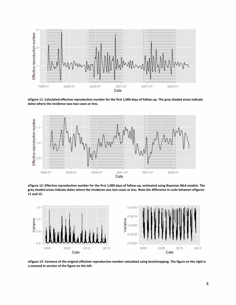
We calculated the variance of 𝑅(𝑡) by taking 1,000 bootstrapping samples of the weekly incidence data.
For each sample, we calculated 𝑅(𝑡) as above. During periods of low incidence, we observed a larger
degree of uncertainty in the effective reproduction number than during periods of higher incidence
7
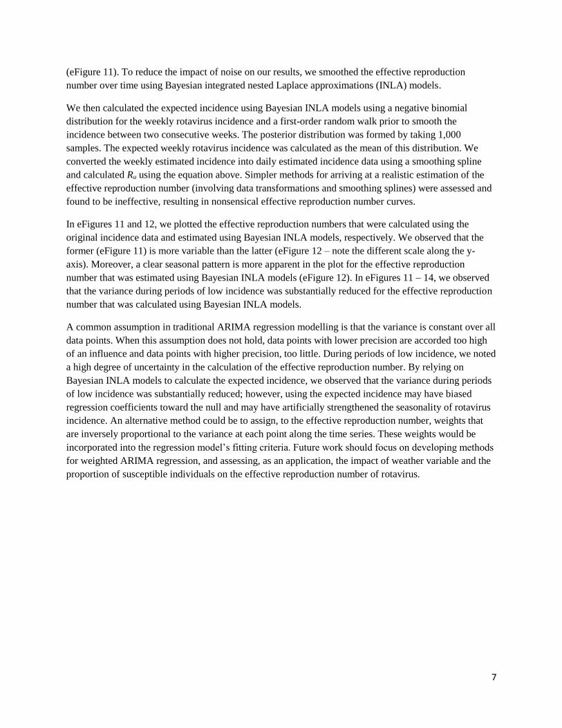
(eFigure 11). To reduce the impact of noise on our results, we smoothed the effective reproduction
number over time using Bayesian integrated nested Laplace approximations (INLA) models.
We then calculated the expected incidence using Bayesian INLA models using a negative binomial
distribution for the weekly rotavirus incidence and a first-order random walk prior to smooth the
incidence between two consecutive weeks. The posterior distribution was formed by taking 1,000
samples. The expected weekly rotavirus incidence was calculated as the mean of this distribution. We
converted the weekly estimated incidence into daily estimated incidence data using a smoothing spline
and calculated Ru using the equation above. Simpler methods for arriving at a realistic estimation of the
effective reproduction number (involving data transformations and smoothing splines) were assessed and
found to be ineffective, resulting in nonsensical effective reproduction number curves.
In eFigures 11 and 12, we plotted the effective reproduction numbers that were calculated using the
original incidence data and estimated using Bayesian INLA models, respectively. We observed that the
former (eFigure 11) is more variable than the latter (eFigure 12 – note the different scale along the y-
axis). Moreover, a clear seasonal pattern is more apparent in the plot for the effective reproduction
number that was estimated using Bayesian INLA models (eFigure 12). In eFigures 11 – 14, we observed
that the variance during periods of low incidence was substantially reduced for the effective reproduction
number that was calculated using Bayesian INLA models.
A common assumption in traditional ARIMA regression modelling is that the variance is constant over all
data points. When this assumption does not hold, data points with lower precision are accorded too high
of an influence and data points with higher precision, too little. During periods of low incidence, we noted
a high degree of uncertainty in the calculation of the effective reproduction number. By relying on
Bayesian INLA models to calculate the expected incidence, we observed that the variance during periods
of low incidence was substantially reduced; however, using the expected incidence may have biased
regression coefficients toward the null and may have artificially strengthened the seasonality of rotavirus
incidence. An alternative method could be to assign, to the effective reproduction number, weights that
are inversely proportional to the variance at each point along the time series. These weights would be
incorporated into the regression model’s fitting criteria. Future work should focus on developing methods
for weighted ARIMA regression, and assessing, as an application, the impact of weather variable and the
proportion of susceptible individuals on the effective reproduction number of rotavirus.
8
eFigure 11: Calculated effective reproduction number for the first 1,000 days of follow-up. The grey shaded areas indicate dates where the incidence was two cases or less.
eFigure 12: Effective reproduction number for the first 1,000 days of follow-up, estimated using Bayesian INLA models. The grey shaded areas indicate dates where the incidence was two cases or less. Note the difference in scale between eFigures 11 and 12.
eFigure 13: Variance of the original effective reproduction number calculated using bootstrapping. The figure on the right is a zoomed-in version of the figure on the left.

9
A brief note on the challenges in estimating birth rates and incidence
Birth rates for the population yielding rotavirus incidence data were unavailable for two reasons. (i) Only
a small proportion of laboratories in the Netherlands report to the NWKV database, therefore not all
individuals in the Netherlands who test positive for rotavirus are included in the database. This implies
that using country-wide birth rates would have grossly overestimated the proportion of susceptible
individuals. (ii) The catchment area of the laboratories that submit rotavirus incidence data to the NWKV
on any given week and from week-to-week was unknown. This implies that we could not determine the
birth rate for only the regions from which the cases originated. Estimating the number of individuals in
the catchment area that were infected at any given time is challenging. Laboratory tests are not conducted
on all individuals with rotavirus since not all primary infections are symptomatic, not all symptomatic
cases are serious enough to lead caregivers to seek medical care, and not all individuals who seek medical
care are tested. For these reasons, we relied on reported weekly incidence statistics to inform our estimate
of the true weekly incidence of the entire populations of the Netherlands.
Moving average of the results of the regression model
In our results, we found that the proportion of susceptible individuals, mean temperature, and seasonal
effects alone did not completely capture the week-to-week variability in the effective reproduction
number. We hypothesized that a moving average of these factors should capture the moving average
trends of R(t). Where these two moving averages diverge from one another should highlight time periods
where the most important model improvements could be made.
In preliminary analyses, we separately averaged the model estimate and R(t) over n=2,3,…,52
consecutive weeks. We found that a 28-week moving average yielded the lowest least-squares fit of the
model estimate to R(t). Using this 28-week moving average, we that transmission during the summer
months and the rotavirus season in 2014 could be better explained, implying other sources of, or causes of
reduced, transmission.
eFigure 14: Variance of the estimated effective reproduction number calculated using Bayesian INLA methods. The figure on the right is a zoomed-in version of the figure on the left.

10
Time series data used in our analyses
In the following figure, we present the weekly data used in our main analyses. Only factors that were
shown to be associated with the log effective reproduction number (i.e., (b) and (c)) were included in our
final model.

11

12
eFigure 15: Time series data used in our analysis. (a) The outcome on the natural scale – weekly average effective reproduction number. Figures (b) – (f) show the different factors, average by week, that we assessed for their association with the outcome: (b) the proportion of susceptible individuals, shown on the natural scale, (c) the minimum (black), mean (red), and maximum (black) temperature, (d) the minimum (black), mean (red), and maximum (black) absolute humidity, (e) ultraviolet light, and (f) rainfall.

13
References
Centers for Disease Control and Prevention. Rotavirus: Epidemiology and Prevention of Vaccine
Preventable Diseases. The Pink Book: Course Textbook - 12th Edition Second Printing (May 2012).
http://www.cdc.gov/vaccines/pubs/pinkbook/rota.html. Accessed May 15, 2015.
Kenah E, Lipsitch M, Robins JM. Generation interval contraction and epidemic data analysis. Math
Biosci. 2008; 213: 71-79.
Lopman B, Vicuña Y, Salazar F, Broncano N, Esona MD, et al. Household Transmission of Rotavirus in
a Community with Rotavirus Vaccination in Quininde, Ecuador. PLoS ONE. 2013; 8(7): e67763.
Vink MA, Bootsma MCJ, Wallinga J. Serial Intervals of Respiratory Infectious Diseases: A Systematic Review and Analysis. Am J Epidemiol. 2014; 180 (9): 865-875.

14
C. Example code for ARIMA models with non-linear distributed lags.
outcome <- <outcome.of.interest>
ef <- <external.factor>
knots <- c(<where.would.you.like.the.knots.to.go>)
n.lags <- number.of.lags
var.ef <- number.of.degrees.of.freedom.for.external.factor
dlnm.ef <- crossbasis(ef,
lag=n.lags, arglag=list(fun="ns", knots=knots),
argvar=list(fun="ns", df=var.ef))
dimnames(dlnm.ef)[[2]] <- paste(".ef", dimnames(dlnm.ef)[[2]], sep=".")
arima.model <- Arima(outcome, order=c(p,0,q), seasonal=list(order=c(P,0,Q),
period=7), xreg=cbind(dlnm.ef, <other external factor(s)>, sin(t),
cos(t)))
test <- crosspred(dlnm.ef, coef=arima.model$coef[grepl("ef",
names(arima.model$coef))], vcov=arima.model$var.coef[grepl("ef",
dimnames(arima.model$var.coef)[[1]]), grepl("ef",
dimnames(arima.model$var.coef)[[2]])], by = 0.1)
test$model.class <- "lm"
test$model.link <- "identity"
plot(test, lag=i)
plot(test, var=i)
15
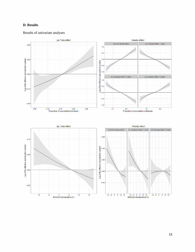
D. Results
Results of univariate analyses

16
17
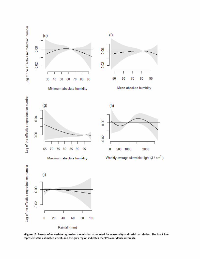
eFigure 16: Results of univariate regression models that accounted for seasonality and serial correlation. The black line represents the estimated effect, and the grey region indicates the 95% confidence intervals.
18
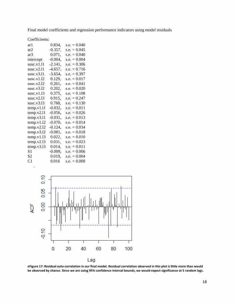
Final model coefficients and regression performance indicators using model residuals
Coefficients:
ar1
ar2
ar3
intercept
susc.v1.l1
susc.v2.l1
susc.v3.l1
susc.v1.l2
susc.v2.l2
susc.v3.l2
susc.v1.l3
susc.v2.l3
susc.v3.l3
temp.v1.l1
temp.v2.l1
temp.v3.l1
temp.v1.l2
temp.v2.l2
temp.v3.l2
temp.v1.l3
temp.v2.l3
temp.v3.l3
S1
S2
C1
0.834,
-0.357,
0.071,
-0.004,
-2.141,
-4.657,
-3.654,
0.129,
0.261,
0.202,
0.375,
0.915,
0.768,
-0.032,
-0.056,
-0.031,
-0.070,
-0.124,
-0.081,
0.022,
0.031,
0.014,
-0.009,
0.019,
0.016
s.e. = 0.040
s.e. = 0.045
s.e. = 0.040
s.e. = 0.004
s.e. = 0.306
s.e. = 0.716
s.e. = 0.397
s.e. = 0.017
s.e. = 0.041
s.e. = 0.020
s.e. = 0.108
s.e. = 0.247
s.e. = 0.130
s.e. = 0.011
s.e. = 0.026
s.e. = 0.013
s.e. = 0.014
s.e. = 0.034
s.e. = 0.018
s.e. = 0.010
s.e. = 0.023
s.e. = 0.011
s.e. = 0.006
s.e. = 0.004
s.e. = 0.008
.
eFigure 17: Residual auto-correlation in our final model. Residual correlation observed in this plot is little more than would be observed by chance. Since we are using 95% confidence interval bounds, we would expect significance at 5 random lags.

19
eFigure 18: Q-Q plot of the residuals of our final model.

20
Comparing results of different multivariate models
In eTable 2, we compared across alternative multivariate models that included different lags for mean
temperature and the proportion of susceptible individuals the model fit according to the Akaike
Information Criteria (AIC) and Bayesian Information Criteria (BIC). These multivariate models
incorporated coefficients and lagged factors using natural cubic splines with three degrees of freedom and
accounted for seasonality and serial correlation. This does not represent an exhaustive list of all the
models that were tested as we also tested models where factors were included with different functional
forms and different degrees of freedom. Models with variables included with one lag resulted in
singularities and results for these models were therefore not computable.
We observed that the model with the best fit according to the AIC was the model with two lags for mean
temperature and three lags for the proportion of susceptible individuals (model 7). This model had the
second best fit according to the BIC, and was selected as our final model in the main manuscript.
According to the BIC, the best model included mean temperature only as an immediate variable and the
proportion of susceptible individuals with three lags (model 3). This model had the third best fit according
to the AIC.
Results of these two multivariate models, along with the model with no lagged factors (model 1), reveal a
similar direction of the estimated effect of mean temperature and the proportion of susceptible individuals
(eFigures 19-21). The best fitting model according to the AIC (model 7), suggested an effect of mean
temperature that is nearly significantly larger than that of the two other models (eFigure 21 vs. eFigures
19 and 20).
eTable 2: Comparison of Akaike Information Criteria (AIC) and Bayesian Information Criteria (BIC) across different lags for mean temperature and the proportion of susceptible individuals. These factors were included simultaneously in a multivariate model that accounted for seasonality and serial correlation.
Lags included in multivariate model
Model Mean
temperature
Proportion of
susceptible individuals
AIC BIC
1 0 0 -3617 -3551
2 2 -3655 -3561
3 3 -3681 -3587
4 4 -3646 -3552
5 2 0 -3620 -3526
6 2 -3667 -3544
7 3 -3696 -3573
8 4 -3656 -3533
9 3 0 -3613 -3519
10 2 -3659 -3536
11 3 -3692 -3569
12 4 -3654 -3531

21
eFigure19: Multivariate model including only the immediate effect of factors, and accounting for seasonality and serial correlation. The black line represents the estimated effect, and the grey region indicates the 95% confidence intervals.
eFigure 20: Multivariate model including the immediate effects of mean temperature and the proportion of susceptible individuals, as well as three lagged terms for the proportion of susceptible individuals. This model accounted for seasonality and serial correlation. The black line represents the estimated effect, and the grey region indicates the 95% confidence intervals.

22
eFigure 21: Multivariate model including the immediate effects of mean temperature and the proportion of susceptible individuals, as well as three lagged terms for both mean temperature and the proportion of susceptible individuals. This model accounted for seasonality and serial correlation. The black line represents the estimated effect, and the grey region indicates the 95% confidence intervals. (This is the same as Figure 4 in the main manuscript.)

23
E. Sensitivity analyses
Varying the average duration in the susceptible class used in local linear regression that estimates the
proportion of susceptible individuals over time
We varied the average duration in the susceptible class from 9 months to 3 months, 15 months, and 30
months, and recomputed our results, keeping the number of lag terms constant throughout. We can see
that decreasing or increasing the average duration in the susceptible class does slightly influence the
estimates of the proportion of susceptible individuals over time (eFigure 22). The week-to-week effects
are sensitive to the selection of the average duration in the susceptible class, hinting at overfitting of these
week-to-week effects, at least in terms of this variable. Nevertheless, we only observe a reduction in the
total effect of the proportion of susceptible individuals when the average duration in the susceptible class
is 3 months (eFigures 23-26).

24
eFigure 22: Proportion of susceptible individuals over time. The average duration in the susceptible class used to estimate the proportion of case ascertainment was (a) 3 months, (b) 9 months, (c) 15 months, and (d) 30 months.
(c)
(b)
(d)
(a)
25
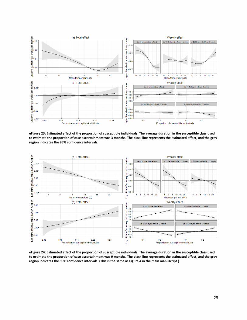
eFigure 23: Estimated effect of the proportion of susceptible individuals. The average duration in the susceptible class used to estimate the proportion of case ascertainment was 3 months. The black line represents the estimated effect, and the grey region indicates the 95% confidence intervals.
eFigure 24: Estimated effect of the proportion of susceptible individuals. The average duration in the susceptible class used to estimate the proportion of case ascertainment was 9 months. The black line represents the estimated effect, and the grey region indicates the 95% confidence intervals. (This is the same as Figure 4 in the main manuscript.)
26
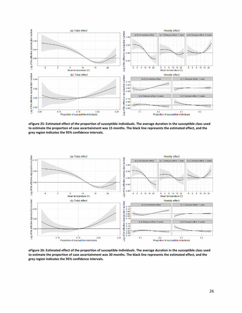
eFigure 25: Estimated effect of the proportion of susceptible individuals. The average duration in the susceptible class used to estimate the proportion of case ascertainment was 15 months. The black line represents the estimated effect, and the grey region indicates the 95% confidence intervals.
eFigure 26: Estimated effect of the proportion of susceptible individuals. The average duration in the susceptible class used to estimate the proportion of case ascertainment was 30 months. The black line represents the estimated effect, and the grey region indicates the 95% confidence intervals.

27
Testing the sensitivity of our results to a longer serial interval
We tested the sensitivity of our results to a longer serial interval by increasing the mean of 2.1 days to
approximately seven days. We both stretched (mean = 6.9, sd = 4.6) and shifted (mean=7.1, sd = 0.9) our
original serial interval and tested the sensitivity of our results (eFigure 27) to these new distributions.
When stretched, temperature only seems to be slightly affected, whereas the effect of the proportion of
susceptible individuals nearly increases by a factor of two or three (eFigure 28). When shifted, both the
effects of temperature and the proportion of susceptible individuals nearly increase by a factor of two or
three (eFigure 29). These results are expected. An increase in the mean time between successive cases is
expected to increase the magnitude of the estimated effective reproduction number, while reducing
variability (and precision if the true serial interval is indeed shorter). Therefore, while a weaker
association could disappear due to the reduction in variability, we would expect a stronger association to
be amplified to reflect increases in the estimated effective reproduction number.
eFigure 27: Results corresponding to our original serial interval. The black line represents the estimated effect, and the grey region indicates the 95% confidence intervals. (This is the same as Figure 4 in the main manuscript.)

28
eFigure 28: Results corresponding to a stretched distribution. The black line represents the estimated effect, and the grey region indicates the 95% confidence intervals.
eFigure 29: Results corresponding to a shifted distribution. The black line represents the estimated effect, and the grey region indicates the 95% confidence intervals.

29
Testing the sensitivity of our results of incomplete immunity
We tested the sensitivity of our results to incomplete immunity such that reported cases included
reinfections. We assumed that individuals were not always removed from the population of interest once
they became infected, and were considered as susceptible again in the following year/season.
Modifications made to our methods to reflect incomplete immunity from severe infection included
adjusting the local regression and the balance equation for the number of susceptible individuals (page 4
of the manuscript). For local regression, we added to the susceptible individuals the fraction of
individuals that remained susceptible to a severe infection after a previous severe infection, delayed for a
period to reflect the fact that individuals were unlikely to have a second severe infection during the same
rotavirus season. This modification to the local regression equation generated a new estimate of the
proportion of case ascertainment, 𝛼𝑚(𝑖), that was then used directly in the balance equation that
estimated the number of susceptible individuals. In addition, this equation was modified to reflect the fact
that (a fraction, 𝛾, of) infected individuals once again re-entered the susceptible class after a delay of 𝜌
days:
𝑆(𝑡) = 𝑆0 + ∑ [𝛿(𝑖) +𝛾
𝛼𝑚(𝑖)∙ 𝐼𝑟(𝑖 − 𝜌) −
1
𝛼𝑚(𝑖)∙ 𝐼𝑟(𝑖)] 𝑡
𝑖=1 .
Here, we allowed for 15% of the individuals infected in any given year to be included in the susceptible
population again six months later – preventing the opportunity for reinfection during the same rotavirus
season, but allowing reinfection in the following rotavirus season or at any time thereafter. We found that
our results were sensitive to allowing 15% of the infected individuals to re-enter the susceptible
population 6 months after infection (eFigure 31).
eFigure 30: Original results presented in the Figure 4 of the main manuscript. The black line represents the estimated effect, and the grey region indicates the 95% confidence intervals.

30
eFigure 31: Results corresponding to incomplete immunity. The black line represents the estimated effect, and the grey region indicates the 95% confidence intervals.