A Price Theory of Vertical and Lateral Integration∗

Patrick Legros† Andrew F. Newman‡

March 2009; revised April 2012

Abstract

We present a perfectly-competitive model of firm boundary decisions and study

their interplay with product demand, technology, and welfare. Integration is privately

costly but is effective at coordinating production decisions; non-integration will coor-

dinate less effectively and will have lower costs, especially if surplus is shared equally.

Output price influences the choice of ownership structure: integration increases with

the price level. Ownership in turn affects output, since integration is more productive

than non-integration. The model generates robust coexistence of different ownership

structures among ex-ante identical enterprises. The price mechanism correlates reorga-

nizations across firms and generates external effects of technological shocks: productiv-

ity changes in some firms may induce changes of ownership in the rest of the industry.

If the managers choosing organizational design have full claim to enterprise revenues,

market equilibrium ownership structures will be second-best efficient. When managers

have less than a full claim on revenue, equilibrium can be inefficient, with too little

integration. We discuss some recent examples from the empirical literature in light of

the model.

∗We are grateful for helpful discussion with Roland Benabou, Patrick Bolton, Phil Bond, Estelle Cantil-

lon, Paola Conconi, Jay Pil Choi, Mathias Dewatripont, Robert Gibbons, Ricard Gil, Oliver Hart, Bengt

Holmstrom, Kai-Uwe Kuhn, Giovanni Maggi, Armin Schmutzler, George Symeonidis, four anonymous refer-

ees and the editors of this journal, and workshop participants at Boston University, Washington University,

ESSET Gerzensee, the Harvard/MIT Organizational Economics Seminar, the NBER ITO Working Group,

and Toulouse. Legros benefited from the financial support of the Communaute Francaise de Belgique

(projects ARC 98/03-221 and ARC00/05-252), and EU TMR Network contract no FMRX-CT98-0203.†ECARES, Universite libre de Bruxelles, ECORE and CEPR.‡Boston University and CEPR.

1

1 Introduction

While it is clear to most economists that organizational design is crucial for the behavior

of the business firm, there appears to be rather less consensus on whether it matters at the

level of the industry. Indeed, the field of Industrial Economics, which at bottom is the study

of how firms deliver the goods, has been largely content to ignore the internal organization

of its key protagonists. The stage on which they perform, the imperfectly competitive

market, dominates the show. There are good reasons for this. Analytical parsimony is one.

More fundamental is the presumption that departures from Arrow-Debreu behavior by the

individual firm will be weeded out by the discipline of competition: in effect, imperfection

in the market is the root of all distortion. What is missing to challenge this view is

a clear demonstration thatimperfections within firms can, by themselves, affect industry

conduct and performance. In other words, if organizational design matters for the concerns

of industrial economics, its impact ought to be apparent in the simplest of all industrial

models, perfect competition.

This paper provides such a model and shows that internal organization — specifically

ownership and control in the incomplete-contract tradition of Grossman-Hart (Grossman

and Hart 1986, Hart and Moore 1990) — has distinctive positive and normative implica-

tions for industry behavior. It presents a simple textbook-style industry model in which

“neoclassical black-box” firms are replaced by partnerships of manager-led suppliers who

choose ownership structures to govern trade-offs between private costs and coordination

benefits. All other aspects of the model are standard for perfect competition: enterprises

and consumers are price takers, the formation of the partnerships between suppliers is

frictionless, and entry is allowed.

The organizational building block at the heart of our analysis is an adaptation of the

model in Hart and Holmstrom (2010). In order to produce a unit of the consumer good, two

complementary suppliers, each consisting of a manager and his collection of assets, must

enter into a relationship. The managers operate the assets by making non-contractible

production decisions. Technology requires mutual compatibility of the decisions made for

different parts of the enterprise.

The problem is that decisions that are convenient for one supplier will be inconvenient

for the other, and vice versa, which generates private costs for each manager. This incom-

patibility may reflect a technological need for adaptability (the BTU and sulphur content

of coal needs to be optimally tailored to a power plant’s boiler and emissions equipment),

or occupational backgrounds (engineering favors elegant design and low maintenance; sales

prefers redundant features and user-friendliness). Each party will find it costly to accom-

modate the other’s approach, but if they don’t agree on something, the enterprise will be

poorly served.

The main organizational decision the managers have to make is whether to integrate. If

they retain control over their assets and subsequently make their decisions independently,

2

this may lead to low levels of output, since they overvalue the private costs and are apt

to be poorly coordinated. Integration addresses this difficulty via a transfer of control

rights over the decisions to a third-party “HQ,” who, like the managers, enjoys profit, but

unlike them, has no direct concern for the decisions. Since HQ will have a positive stake

in enterprise revenue, she maximizes the enterprise’s output by enforcing a compatible

decision. The cost of this solution is that the compromise standard will be inconvenient to

both managers.

The industry is composed of a large number of suppliers of each type who form en-

terprises in a matching market, at which time they decide whether to integrate and how

to share revenues. The industry supply curve will embody a relationship between the

price and ownership structure, as well as the usual price-quantity relationship. Once this

“Organizationally Augmented Supply” curve (OAS) has been derived, it is feasible to per-

form a textbook-style supply-and-demand analysis of both the comparative statics and the

economic performance of equilibrium ownership structures.

One set of findings concerns the positive implications of the structure of the OAS.

First is the relationship between market price and ownership structure. At low prices,

managers do not value the increase in output brought by integration since they are not

compensated sufficiently for the high costs they have to bear. At higher prices, managers

value output so much that they are willing to forgo their private interests in order to

achieve coordination, and therefore choose to integrate. Thus, demand matters for the

determination of equilibrium ownership structure, because it helps determine the market

price. As product price is common to a whole industry, the price mechanism provides

a natural impetus toward widespread, demand-induced restructuring, as in “waves” of

mergers or divestitures.

Second, product price is also a key source of “external” influence on organizational

design, which raises the possibility of supply-induced restructuring. For instance, techno-

logical shocks that occur in a few firms will affect market price and therefore potentially

the ownership choice of many other firms. One implication of this external effect is that

positive technological progress may have little impact on aggregate performance because

of “re-organizational absorption”: the incipient price decrease from increased productiv-

ity among some firms may induce the remaining firms to choose non-integration, thereby

lowering their output and keeping industry output unchanged.

Third is a theory of heterogeneity in ownership structure and performance. Endogenous

coexistence of different ownership structures, even among firms facing similar technology, is

a generic outcome of market equilibrium. The heterogeneity is an immediate consequence

of the productivity difference between integration and non-integration: while managers

may be indifferent between the two, integration produces more output. Thus if per-firm

demand is in between the output levels associated with each ownership structure, there

must be a mixture of the two in equilibrium. In this part of the supply curve, changes in

demand are accommodated less by price adjustments than by ownership changes.

3

These findings help us interpret some recent empirical findings on the determinants of

ownership structure and performance in the air travel and ready-mix concrete industries.

Evidence on air travel corroborates our basic result relating integration to product price.

As described by Forbes-Lederman (2009, 2010), the tendency for major airlines to own local

carriers is greatest in markets where routes are most valuable. Interpreting product price as

the measure of value, this reflects the above-mentioned dependence of integration on price

that characterizes demand-driven restructuring. In the concrete industry, Hortacsu and

Syverson (2007) show that enterprises with identical technology make different integration

choices, a finding that is difficult to reconcile with a model of integration that is based

only on technological considerations, but is easily understood in terms of our heterogeneity

result. Moreover, their other findings, which relate price and the degree of integration in

the market, are explained in terms of supply-driven restructuring.

The model is amenable to simple consumer-producer surplus calculations, from which

we derive two main welfare results. We show first that the competitive equilibrium is

“ownership efficient,” as long as managers fully internalize the effect of their decisions on

the profit, as in small or owner-managed firms. That is, a planner could not increase the

sum of consumer and producer surplus by forcing some enterprises to re-organize.

However, for firms in which the managers’ financial stakes are lower, there is always a

set of demand functions for which equilibria are ownership inefficient. Specifically, since

integration favors consumers because it produces more than non-integration, inefficiencies

assume the form of too little integration: managers without full financial stakes overvalue

their private costs. By analogy to the Harberger triangle measure of deadweight loss

from market power, we identify a “Leibenstein trapezoid” that measures the extent of

organizational deadweight loss. In contrast to the case of market power in which welfare

losses are greatest when demand is least elastic, we show that organizational welfare losses

are greatest when demand is most elastic.

These welfare losses are unlikely to be mitigated by instruments that reduce frictions.

Indeed, if managers have access to positive cash endowments or can borrow the cash with

which to make side payments to each other, they are more likely to adopt non-integration,

which hurts consumers. This result offers a new perspective on the costs of “free cash flow”:

managers use it to pursue their private interests, but here it may take the form of too little

rather than too much integration. In a similar vein, free entry into the product market

does not significantly affect results: the “long run” OAS typically has a similar shape to

the short run OAS, in particular admitting generic heterogeneity, and the long-run welfare

results parallel those of the short run.

Literature

Our paper is related to a line of research on the effect of the degree of competition on man-

agerial incentives (Machlup 1967, Hart 1983, Sharfstein 1988, in a competitive setting; and

4

Schmidt 1997, Fershtman and Judd 1987, and Raith 2003 in an imperfectly competitive

framework). The focus there is on the power of compensation schemes, leaving organiza-

tional design (and firm boundaries in particular) exogenous. There is also a literature that

relates market forces and investment in monitoring technologies (Banerjee and Newman

1993, Legros and Newman 1996), but allocations of decision rights, firm boundaries and

ownership are not considered.

Our earlier work on the external determinants of ownership structure (Legros and

Newman 2008) studies how relative scarcities of different types of suppliers determine the

allocation of control. It does not consider the effects of the product market, nor does it

consider consumer welfare.

Marin and Verdier (2008) and Alonso et al. (2008) consider models of delegation in

different imperfect competition settings; firm boundaries are fixed in these models and the

issue is whether information acquisition is facilitated by delegated or centralized decision

making. Gibbons, Holden and Powell (2011) consider a model in which the ownership

decision is the means by which firms acquire information about an aggregate state, but

that information is also incorporated into market prices. Rational expectations equilibrium

entails heterogeneity of ownership structure, with some firms acquiring information and the

rest inferring it from prices.

McLaren (2000) and Grossman and Helpman (2002) develop search models to explain

the pattern of outsourcing in industries when there is incomplete contracting (see also

Antras 2003, Antras and Helpman 2004). These papers proceed somewhat more in the

Williamsonian tradition, where integration alleviates the hold-up problem at an exogenous

fixed cost. McLaren (2000) shows that globalization, interpreted as market thickening,

leads to non-integration and outsourcing. Grossman and Helpman (2002) develop simi-

lar tradeoffs in a monopolistic competition model with free entry, and use it to address

more industrial organization questions like the effect of demand elasticity (or degree of

competition) on organizational choice and to address the possibility of heterogeneity in

organizational choices. Imperfect competition and search frictions nevertheless make it

difficult to isolate the pure organization effects on consumer welfare.

Our perfectly competitive framework enables us to address these welfare questions, to

generate a simple account of organizational heterogeneity, to generate predictions about

the relationships between price levels and integration and to give a treatment about an or-

ganizational industry response to technological changes. It points to a two-way interaction

between profitability and integration decisions (at the individual firm level) and between

price and integration at the industry level (Powell 2011 explores a similar interaction in

the context of relational contracting). It also points to issues that have not received much

treatment in the organizational IO literature such as the role of corporate governance on

consumer welfare, and the connection among industry performance, finance, ownership

structure that stands in contrast to the strategic use of debt that has been studied in the

literature (e.g., Brander and Lewis 1986).

5

Finally, the possibility that firms may persistently underperform, even in the face of

competition, owes something to the “X-inefficiency” tradition started by Leibenstein (1966;

see also Bertrand and Mullainathan, 2003). In our model, the ownership decision deter-

mines the extent to which managerial slack can be sustained in the organization: non-

integrated firms allow managers to live the quiet life if they so desire, something that in-

tegration precludes. Much as Leibenstein argued, and as we quantify with the eponymous

trapezoid, our analysis suggests that the welfare losses from this kind of organizational

inefficiency might be significant.

2 Model

This section presents the basic model, where managers are full claimants to the revenue.

The basic organizational building block is a single-good, continuous-action version of Hart

and Holmstrom’s (2010) model. The aim is to derive an industry supply curve that summa-

rizes the relationships among price, quantity and ownership structure. This is best thought

of as a “short run” supply curve, for which entry into the industry is limited. Discussion

of entry and long-run supply is deferred to section 5.

2.1 Environment

Technology, Preferences and Ownership Structures

There is one consumer good, the production of which requires the coordinated input of

one A and one B. Call their union an “enterprise.” Each supplier can be thought of as

collection of assets and workers, overseen by a manager, that cannot be further divided

without significant loss of value. Examples of A and B might include “lateral” relationships

such as manufacturing and customer support, as well as vertical ones such as microchips

and computers. The industry will be comprised of a large number of each type of supplier,

but for the moment confine attention to a single pair.

For each supplier, a non-contractible decision is rendered indicating the way in which

production is to be carried out. For instance, networking software and routing equipment

could conform to many different standards; material inputs may be well- or ill-suited to

an assembler’s production machinery. Denote the decision in an A supplier by a ∈ [0, 1],

and a B decision by b ∈ [0, 1]. The decision might be made by the supplier’s manager, but

could also be made by someone else, depending on the ownership structure, as described

below.

As the examples indicate, these decisions are not ordered in any natural way; what is

important for expected output maximization is not which particular decision is made in

each part of the enterprise, but rather that it is coordinated with the other. Formally,

the enterprise will succeed, in which case it generates 1 unit of output, with probability

1− (a− b)2; otherwise it fails, yielding 0.

6

The manager of each supplier is risk-neutral and bears a private (non-contractible) cost

of the decision made in his unit. The managers’ payoffs are increasing in income, but they

disagree about the direction decisions ought to go: what is easy for one is hard for the

other, and vice versa. Specifically, we assume that the A manager’s utility is yA− (1−a)2,

and the B manager’s utility is yB−b2, where yA and yB are the respective realized incomes.

A manager must live with the decision once it is made: his function is to implement it

and convince his workforce to agree; thus regardless of who makes a decision, the manager

bears the cost.1

Managers have limited liability (thus yA ≥ 0, yB ≥ 0) and do not have any means

of making fixed side payments, that is, they enter the scene with zero cash endowments.

The significance of this assumption is that the equilibrium division of surplus between

the managers, which is determined in the supplier market, will influence the choice of

ownership structure. By contrast, if cash endowments were sufficiently large, the “ most

efficient” ownership structure (from the managers’ point of view) would always be chosen,

independent of supplier market conditions. We consider arbitrary finite cash endowments

in Section 5.

The ownership structure can be contractually assigned. Here there are two options;

following the property rights literature, each implies a different allocation of decision mak-

ing power. First, the production units can remain two separate firms (non-integration), in

which case the managers retain control over their respective decisions. Alternatively, the

managers can integrate into a single firm, re-assigning control in the process. They do so

by selling the assets to a headquarters (HQ), empowering her to decide both a and b and

at the same time giving her title to (part of) the revenue stream.2 We assume that HQ’s

always have enough cash to finance the acquisition.

HQ’s payoff is simply her income yH ≥ 0; thus she is motivated only by monetary

concerns and incurs no direct cost from the a and b decisions, which are always borne by

the managers of the two units. As a self-interested agent, HQ can no more commit to a pair

of decisions (a, b) than can A and B. Integration simply trades in one incentive problem

for another.3

1Thus, the cost function need not be a characteristic of the individual manager, although that is oneinterpretation, so much as an inherent property of the type of input or employee he oversees: if the managersswitched assets, they’d “switch preferences” (as happens when a professor of economics becomes a dean ofa business school). We expect very similar results could also be generated by a model in which managersdiffer in “vision” as in van den Steen (2005).

2In fact, giving HQ the power to decide (a, b) implies that she will get a positive share of the revenue,as we show below.

3An alternate way to integrate would be to have one of the managers — A, say — sell his assets to B.It is straightforward to show (section 2.3) that this form of integration is dominated by other ownershipstructures in this model — the cost imposed on the subordinate manager A is simply too great.

7

Contracts

The enterprise’s revenue is contractible, allowing for the provision of monetary incentives

via sharing rules: any “ budget-balancing” means of splitting the managerial share of

realized revenue is permissible. For the benchmark analysis, assume that the entire revenue

generated by the enterprise accrues to the managers and HQ.4 The assumption will be

relaxed later to allow for the possibility that the managers and HQ accrue only a fraction

of the revenue, the rest of which goes to “shareholders.”

A contract for A,B is a choice of ownership structure and conditional on that a share

of revenues accruing to each manager.

• Under non-integration, a share contract specifies the share s accruing to A when

output is 1; B then gets a share 1− s. By limited liability each manager gets a zero

revenue when output is 0.5

• Under integration, HQ buys the assets A,B for prices of πA and πB in exchange for

a share structure s = (sA, sB, sH) where s ≥ 0 and sA + sB + sH = 1.

The shares of revenue along with the assets prices πA and πB are endogenous, and will be

determined in the overall market equilibrium.

Markets

The product market is perfectly competitive. On the demand side, consumers maximize a

quasilinear utility function taking P as given. This optimization yields a demand D(P ).

Suppliers also take the (correctly anticipated) price P as given when they sign contracts

and make their production decisions.

In the supplier market, there is a continuum of A and B suppliers. In the HQ market,

HQ’s are supplied elastically with an opportunity cost normalized to zero.

4Since there is a single product produced by the enterprise and the revenue from its sale is contractible,it does not matter in which hands the revenue is assumed to accrue initially. A more general formulationwould suppose that the suppliers produce complementary products (e.g., office suite software and operatingsystems) that generate separate revenue streams, which accrue separately to each supplier; the presentmodel corresponds to the case where these streams are perfectly correlated. A full treatment of that case,which not only admits the possibility of richer sharing rules in which each manager gets a share of the other’srevenue, but also would form the basis for a property-rights theory of multi-product firms, is beyond thescope of this paper, so to speak.

5There is no allowance for third-party budget breakers: as is well known, they can improve performanceonly if they stand to gain when the enterprise fails. (Note also that because output in case of failure isequal to zero, budget breaking is not effective when managers have zero cash endowments.) For simplicity,borrowing from third parties to make side payments is also not allowed; relaxation of this assumption isdiscussed in Section 5.

8

2.2 Equilibrium

There are three types of enterprises that correspond to the formation of the following

coalitions:6

• Single agent coalitions, the feasible set of payoffs for which are independent of the

product market price and coincide with payoffs lower than an exogenous opportunity

cost. The opportunity cost of HQ’s is equal to zero, but the opportunity cost of

other agents may be positive.

• Coalitions consisting of one A supplier and one B supplier. The feasible set for

these coalitions will depend, among other things, on the product market price and

corresponds to the set of payoffs that are achievable through contracts when supplier

A has ownership of asset A and supplier B has ownership of asset B.

• Coalitions consisting of one A supplier, one B supplier and a HQ. The feasible set

for these coalitions will depend on the product market price and corresponds to the

set of payoffs that are achievable through contracts where HQ has ownership of the

assets of A,B.

The feasible sets for each enterprise will be derived in the following sections.

For a given coalition, the contract that is chosen determines the decisions that will be

taken and therefore the probability that a positive output is produced by the enterprise.

While output is a random variable at the level of an enterprise, a law of large numbers

implies that at the level of industry output is deterministic. Hence, once coalitions are

formed and contracts agreed upon, there is a well defined industry supply S(P ).

Definition 1. An equilibrium consists of a partition of agents into coalitions, a payoff to

each agent and a product price P such that:

(1) the payoffs to the agents in an equilibrium coalition are feasible given the equilibrium

price P ;

(2) no coalition can form and find feasible payoffs for its members that are strictly greater

than their equilibrium payoffs;

(3) the total supply in the industry S(P ) is equal to the demand D(P ).

2.3 Choice of Organization

Consider a matched pair A and B who will accrue the entire enterprise revenue P in case

of success (0 in case of failure). In order to determine the relative merits of integration and

non-integration and the choice of shares s, they will anticipate their behavior and resulting

6While there are many other potential coalitions, because of the production technology none of themcan achieve payoffs different from what can be achieved by unions of the three we describe.

9

payoffs given each possible contract and choose that which optimizes the payoff of B while

guaranteeing A his equilibrium payoff. To construct the Pareto frontier for A and B, it is

convenient to treat each ownership structure in turn.

Non-integration

Since each manager retains control of his activity, given a share s, A chooses a ∈ [0, 1], B

chooses b ∈ [0, 1]. A’s payoff is (1−(a−b)2)sP−(1−a)2 and B’s is (1−(a−b)2)(1−s)P−b2.The (unique) Nash equilibrium of this game is:

a = 1− s P

1 + Pb = (1− s) P

1 + P. (1)

The resulting expected output is:

QN (P ) ≡ 1− 1

(1 + P )2. (2)

For a given value of s, as the revenue P increases, A and B are willing to concede to

each other’s preferences more (a decreases and b increases). Output is therefore increasing

in the price P : larger values raise the relative importance of the revenue motive against

private costs, and this pushes the managers to better coordinate. The functional forms

generate a convenient property for the model, namely that the output generated under

non-integration does not depend on s, i.e., on how the managers split the firm’s revenue.

This will also be true of integration.

Of course, the managers’ payoffs depend on s; they are:

uNA (s, P ) ≡ QN (P )sP − s2(

P

1 + P

)2

(3)

uNB (s, P ) ≡ QN (P )(1− s)P − (1− s)2(

P

1 + P

)2

. (4)

Varying s, one obtains a Pareto frontier given non-integration. It is straightforward to

verify that it is strictly concave in uA-uB space, a result of the convex cost functions, and

that the total managerial payoff

UN (s, P ) ≡ QN (P )P − (s2 + (1− s)2)(

P

1 + P

)2

(5)

varies from P 2

1+P at s = 0 (or s = 1) to (32 + P )(

P1+P

)2at s = 1/2.

Non-integration has clear incentive problems: A and B managers put too little weight

on the organizational goal in favor of their private benefits. The alternative is integration,

but this introduces other incentive problems: whoever makes the decision will put too

little weight on the private costs. An extreme version of this is when integration gives title

10

to A or B: in this case the decisions made are so costly to the other manager that the

ownership structure is dominated by non-integration. To see this, note that the managerial

surplus under non-integration is always at least UN (0, P ) = P 2/(1 +P ). If B were to have

control (the argument is similar for A), he would choose a and b to maximize his own payoff

(1− (a− b)2)(1− s)P − b2, which entails a = b = 0. This maximizes A’s cost, and the total

surplus is only P − 1, which is less than UN (0, P ). Thus B-control is Pareto dominated by

non-integration, and the only other organizational form of interest is when control is given

to an HQ.

Integration

Consider an integration contract in which the shares of revenue are s = (sA, sB, sH).

Suppose that HQ has financed the asset acquisition with cash.7 Then as long as sH > 0,

HQ will choose to maximize output since her objective function is (1−(a−b)2)sHP . Hence

the decisions that will be taken by an HQ with positive residual rights on revenue must

satisfy a = b; assume that HQ opts for a = b = 1/2, which minimizes the total managerial

cost (1 − a)2 + b2 among all such choices. The cost to each manager is then 1/4. Since

HQ’s compete and have zero opportunity cost, the purchase prices for the assets must total

sHP . Total managerial welfare under integration is therefore U I(P ) ≡ P − 1/2, which is

fully transferable between A and B via adjustments in s or the asset prices. The reason

for transferability is simple: the actions taken and costs borne by A and B do not depend

on their shares. Neither, of course, does integration output.

Notice that the cost of integration is fixed, independent of P . This is a result of the

fact that HQ is an incentive-driven agent who has a stake in the firm’s revenue. If she had

no stake (sH = 0), HQ would be acting as a “disinterested authority,” indifferent among

all decisions (a, b) ∈ [0, 1]2, and hypothetically she could be engaged by the managers to

make the first-best choices.8

The problem with this is that she would be equally happy to choose the “doomsday op-

tion,” setting a = 0, b = 1, thereby inflicting maximal costs on the managers and generating

zero output. For this reason, disinterested authority is not feasible: HQ would always use

the threat of doomsday to renegotiate a zero-share contract to one with a positive share.9

7The appendix A shows that HQ needs to have some cash in order for integration to emerge but thatthe level of cash may be arbitrarily small.

8These maximize (1 − (a − b)2)P − (1 − a)2 − b2, yielding (a∗, b∗) = ( 1+P1+2P

, P1+2P

) (thus a∗ 6= b∗) and

costs 2P2

(1+2P )2, which do depend on P . The first-best surplus is 2P2

1+2P.

9To see how renegotiation works, let the contracted share for HQ be sH = 0 and assume she has beenasked to implement anything other than a = b (in particular, the first-best). After contract signing butbefore making decisions, she makes the following offer: “Give me sH = 1, and I will set a = b = 1/2. If eitherof you rejects, I will keep the original contract (so that neither of you has grounds for a lawsuit), but it willbe doomsday.” This offer is credible because with the original contract, it is optimal for her to implementthe choices she suggests, while with sH = 1, it is optimal to implement a = b = 1/2. The managers thenget −1/4 as continuation payoff if they both accept and −1 if either rejects, making acceptance a weaklydominant strategy of the renegotiation subgame (HQ can make acceptance strictly dominant by offering theequally credible threat to play a = ε, b = 1− ε in case only one manager rejects, and doomsday if they both

11

Anticipating this renegotiated outcome, the managers will give her a positive stake in the

first place.10

Since the decision outcome is the same with any positive share for HQ, and the managers

would always recoup her anticipated revenue via the fixed payments, there is no loss of

generality in assuming that integration contracts give a full share to HQ (s = (0, 0, 1)). She

makes decisions a = b = 1/2, and asset prices are such that πA = uA+ 1/4 and πB = P −πA,

where uA is the equilibrium payoff to A. Hence, the Pareto frontier under integration is

uB = P − 1/2− uA.

Comparison of Ownership Structure

Ownership structure presents a tradeoff. From the A and B managers’ point of view,

integration generates too much coordination relative to the first best; non-integration gen-

erates too little. The choice of ownership structure will depend on distributional as well

as efficiency considerations. Given the product price P, total managerial welfare is con-

stant under integration, independent of how it is distributed, while for non-integration, it

depends on s and therefore on surplus division. In general, neither Pareto dominates the

other, so that supplier market equilibrium, which determines the distribution of surplus

and s, as well as product market equilibrium, which determines P, will both influence the

decision whether to integrate.

The relationship between the individual payoffs and the price has a simple charac-

terization in the managers’ payoff space. Since the minimum non-integration welfare isP 2

1+P (corresponding to s = 0 or 1) exceeds P − 1/2 if and only if P < 1, non-integration

dominates integration at low prices. Because the frontiers are symmetric about uA = uB,

with the integration frontier linear and the non-integration frontier strictly concave, they

intersect twice. The loci of intersections is given by |uA − uB| = P1+P ;11 thus we have:

Proposition 1. (a) Integration is chosen when product price P > 1 and |uA−uB| > P1+P .

(b) Non-integration is chosen when P < 1 or |uA − uB| < P1+P .

(c) Either ownership structure may be chosen when P ≥ 1 and |uA − uB| = P1+P .

do). The offer is also optimal for HQ, since it gives her the largest possible income ex-post. More generally,though the predicted HQ share need not always be equal to one, sH = 0 is never an equilibrium, anddisinterested authority is an impossibility: the first-best cannot be implemented. See Legros and Newman(2012) for a more detailed argument.

10There are of course other reasons why an agent with significant control rights would have a positivestake of contractible revenue. Moral hazard is one: if enforcing the decisions involves any non verifiable cost,giving HQ a large enough share will ensure she acts. Or, if she has an ex-ante positive opportunity cost ofparticipating, the cash-constrained managers would have to give her a positive revenue share to compensate.Finally, the managers could engage in a form of influence activities, lobbying for their preferred outcomeswith shares of revenue.

11To see this, use (3) and (4) to get the absolute difference in payoff |uA − uB | = |2s− 1| P2

P+1; setting

P − 1/2 =(

P1+P

)2

(2 + P − s2 − (1− s)2) to solve for s (solutions exist only for P ≥ 1) gives 2s− 1 = 1/P,

from which the result follows.

12

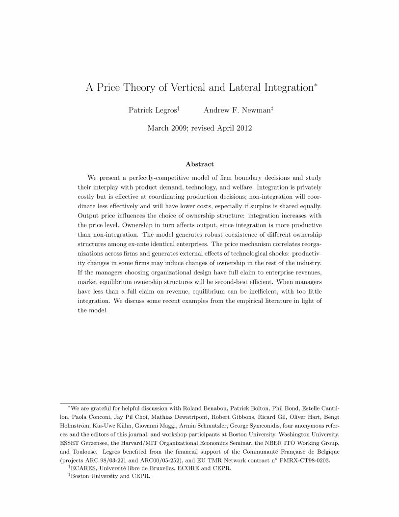
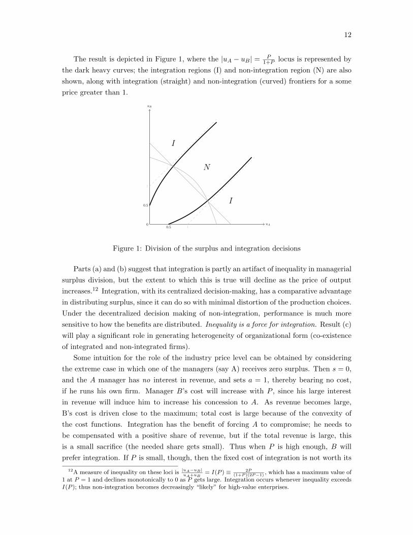
The result is depicted in Figure 1, where the |uA − uB| = P1+P locus is represented by

the dark heavy curves; the integration regions (I) and non-integration region (N) are also

shown, along with integration (straight) and non-integration (curved) frontiers for a some

price greater than 1.

0

uB

uA

1

1

0.5

0.5

N

I

I

Figure 1: Division of the surplus and integration decisions

Parts (a) and (b) suggest that integration is partly an artifact of inequality in managerial

surplus division, but the extent to which this is true will decline as the price of output

increases.12 Integration, with its centralized decision-making, has a comparative advantage

in distributing surplus, since it can do so with minimal distortion of the production choices.

Under the decentralized decision making of non-integration, performance is much more

sensitive to how the benefits are distributed. Inequality is a force for integration. Result (c)

will play a significant role in generating heterogeneity of organizational form (co-existence

of integrated and non-integrated firms).

Some intuition for the role of the industry price level can be obtained by considering

the extreme case in which one of the managers (say A) receives zero surplus. Then s = 0,

and the A manager has no interest in revenue, and sets a = 1, thereby bearing no cost,

if he runs his own firm. Manager B’s cost will increase with P , since his large interest

in revenue will induce him to increase his concession to A. As revenue becomes large,

B’s cost is driven close to the maximum; total cost is large because of the convexity of

the cost functions. Integration has the benefit of forcing A to compromise; he needs to

be compensated with a positive share of revenue, but if the total revenue is large, this

is a small sacrifice (the needed share gets small). Thus when P is high enough, B will

prefer integration. If P is small, though, then the fixed cost of integration is not worth its

12A measure of inequality on these loci is |uA−uB |uA+uB

= I(P ) ≡ 2P(1+P )(2P−1)

, which has a maximum value of1 at P = 1 and declines monotonically to 0 as P gets large. Integration occurs whenever inequality exceedsI(P ); thus non-integration becomes decreasingly “likely” for high-value enterprises.

13

improved output performance, which has little value in the market.

On the other hand if A has a share closer to 1/2, under non-integration he takes account

of the revenue as well as his private costs, and concedes, all the more so as P increases.

The decisions will remain on either side of 1/2 (so output will fall short of the integration

level, but at high revenues this is a small gap), taking account of the private costs, and so

non-integration remains preferable.

The incomplete contracts literature has tended to emphasize the technological (supply-

side) aspects, though distributional aspects have received some attention (Aghion and

Tirole 1994, Legros and Newman 1996, 2008). The present analysis emphasizes the addi-

tional role played by demand, and Proposition 1 illustrates the interplay of demand (P )

and distribution (uA, uB).

2.4 Industry Equilibrium and the “Organizationally Augmented Sup-

ply”

Industry equilibrium comprises a general equilibrium of the supplier, HQ and product

markets. To focus on the role played by market price in determining organizational design,

assume that the suppliers have a zero opportunity cost of participating in this industry and

that the A suppliers are more numerous than the B’s. Thus some of the A’s will remain

unmatched and receive their outside option of 0. Stability then implies that matched A’s

receive 0 as well. In other words, we will be looking along the vertical axis in Figure 1,

where B gets max{uNB (0, P ), uIB(0, P )}. Since uA = 0, proposition 1 implies that there is

indifference between integration and non-integration when P = 1.

To derive the industry supply, suppose that a fraction α of firms are integrated and a

fraction 1 − α are non-integrated. Total supply at price P is then almost surely (because

of the continuum of enterprises and law of large numbers)

α+ (1− α)QN (P ).

When P < 1, α = 0 and total supply is just the output when all firms choose non-

integration. At P = 1, α can assume any value between 0 and 1 since managers are

indifferent between the two forms of organization; however because output is greater with

integration, total supply increases with α. When α = 1 output is 1 and stays at this level

for all P ≥ 1.

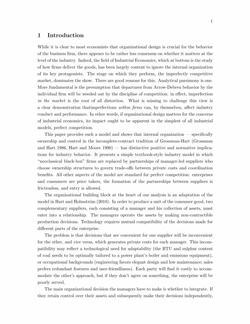
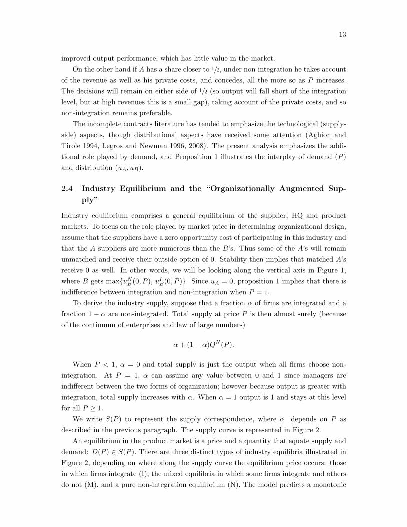
We write S(P ) to represent the supply correspondence, where α depends on P as

described in the previous paragraph. The supply curve is represented in Figure 2.

An equilibrium in the product market is a price and a quantity that equate supply and

demand: D(P ) ∈ S(P ). There are three distinct types of industry equilibria illustrated in

Figure 2, depending on where along the supply curve the equilibrium price occurs: those

in which firms integrate (I), the mixed equilibria in which some firms integrate and others

do not (M), and a pure non-integration equilibrium (N). The model predicts a monotonic

14

Q

P

1

N

M

3/4

I

1

Figure 2: Organizationally Augmented Supply Curve

relationship between the price and integration. As demand increases, the equilibrium price

increases, inducing a greater tendency to integrate.

3 Conduct and Performance of an Organizational Industry

This section emphasizes three consequences of the model pertaining to industry conduct

and performance. First, there is robust coexistence of different ownership structures. Sec-

ond, the organization of one enterprise depends not only on its own technology and man-

agers’ preferences but also on prices determined outside it, implying that “local” changes

can have industry-wide effects. Finally, equilibrium has welfare properties readily charac-

terized in terms of consumer and producer surplus.

3.1 Heterogeneity of Ownership Structure

In the mixed region of the OAS (M) there is coexistence of organizational forms (own-

ership structure) within the industry. Notice that this organizational heterogeneity is an

endogenous consequence of market clearing given a discrete set of ownership structures,

and occurs even though all firms are ex-ante identical.

There is much evidence of productivity variation within industries even among appar-

ently similar enterprises; Syverson (2010) notes that within 4-digit SIC industries in the

U.S. manufacturing sector, a “plant at the 90th percentile of the productivity distribution

makes almost twice as much output with the same measured inputs as the 10th percentile

plant” and that other work on Chinese or Indian firms find even larger differences. More-

over as emphasized by Gibbons (2006, 2010) there is correlation between organizational

15

and productivity variations but there is little theoretical work attempting to explain it.13

The model provides a simple explanation for part of this correlation, since whenever they

coexist, a non-integrated enterprise generates only a fraction of the expected output of an

integrated one.

Observe that while there is only a single price at which the heterogeneous outcome

occurs, it is generated by a generic set of demand functions:

Proposition 2. Consider any demand function D(P ) with that is positive and has finite

elasticity at P = 1. There exists a non-empty open interval (δ, δ) ⊂ R+ such that for any

demand function δD(P ), with δ ∈ (δ, δ) there exists a mix of non-integrated and integrated

firms in equilibrium.

Recall that the pool of HQs is large enough to integrate every enterprise. If instead

the HQs are in short supply, heterogeneity is even more endemic. Indeed, at all prices

exceeding 1, managers would prefer integration if the HQs continued to accrue zero net

surplus, but since there are not enough HQs to go around, some enterprises must be

non-integrated; in equilibrium, HQs extract enough surplus to render managers indifferent

between integration and non-integration.

In contrast to the robust co-existence of ownership structures found here, other papers

investigating endogenous heterogeneity (notably Grossman-Helpman 2002) have found it to

be only non-generic, occurring only for a singular set of parameters. Further consideration

of the difference in results is deferred to the discussion of entry in section 5.

3.2 Heterogeneous Supply Shocks and External Effects

The fact that all enterprises face the same price means that anything that affects it –

a demand shift, foreign competition, or a tax on profits – can lead to widespread and

simultaneous reorganization, as in a merger or divestiture wave. Straightforward demand

and supply analysis can be used to study these phenomena. For instance, growth in demand

might raise the price from below 1 to above it, resulting in a vertical merger wave as firms

switch from non-integration to integration.

By the same token, the organization of a particular enterprise depends not only on its

own technology and managers’ preferences but also on prices (product price and surplus

that managers can obtain by matching with other managers) determined outside it. In

particular, technological “shocks” that directly affect some firms may induce reorganiza-

tions to other firms that are unaffected by the shock, as well as to themselves; in fact,

sometimes only the unaffected firms reorganize, as in the following example.

13An early exception is Hermalin (1994) who obtains heterogeneity in incentive schemes in a principal-agent model when the product market is imperfectly competitive. More recently Gibbons et al. (2011)find heterogeneity in control structures among identical firms in a rational-expectations model where inputprices reveal information.

16

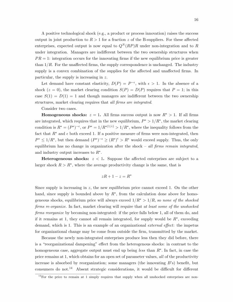
A positive technological shock (e.g., a product or process innovation) raises the success

output in joint production to R > 1 for a fraction z of the B-suppliers. For these affected

enterprises, expected output is now equal to QN (RP )R under non-integration and to R

under integration. Managers are indifferent between the two ownership structures when

PR = 1: integration occurs for the innovating firms if the new equilibrium price is greater

than 1/R. For the unaffected firms, the supply correspondence is unchanged. The industry

supply is a convex combination of the supplies for the affected and unaffected firms. In

particular, the supply is increasing in z.

Let demand have constant elasticity, D(P ) = P−ε, with ε > 1. In the absence of a

shock (z = 0), the market clearing condition S(P ) = D(P ) requires that P = 1; in this

case S(1) = D(1) = 1 and though managers are indifferent between the two ownership

structures, market clearing requires that all firms are integrated.

Consider two cases.

Homogeneous shocks: z = 1. All firms success output is now R∗ > 1. If all firms

are integrated, which requires that in the new equilibrium, P ∗ > 1/R∗, the market clearing

condition is R∗ = (P ∗)−ε, or P ∗ = 1/R∗(1/ε) > 1/R∗, where the inequality follows from the

fact that R∗ and ε both exceed 1. If a positive measure of firms were non-integrated, then

P ∗ ≤ 1/R∗, but then demand (P ∗)−ε ≥ (R∗)ε > R∗ would exceed supply. Thus, the only

equilibrium has no change in organization after the shock – all firms remain integrated,

and industry output increases to R∗.

Heterogeneous shocks: z < 1. Suppose the affected enterprises are subject to a

larger shock R > R∗, where the average productivity change is the same, that is

zR+ 1− z = R∗

Since supply is increasing in z, the new equilibrium price cannot exceed 1. On the other

hand, since supply is bounded above by R∗, from the calculation done above for homo-

geneous shocks, equilibrium price will always exceed 1/R∗ > 1/R, so none of the shocked

firms re-organize. In fact, market clearing will require that at least some of the unshocked

firms reorganize by becoming non-integrated: if the price falls below 1, all of them do, and

if it remains at 1, they cannot all remain integrated, for supply would be R∗, exceeding

demand, which is 1. This is an example of an organizational external effect : the impetus

for organizational change may be come from outside the firm, transmitted by the market.

Because the newly non-integrated enterprises produce less then they did before, there

is a “reorganizational dampening” effect from the heterogenous shocks: in contrast to the

homogeneous case, aggregate output must end up being less than R∗. In fact, in case the

price remains at 1, which obtains for an open set of parameter values, all of the productivity

increase is absorbed by reorganization; some managers (the innovating B’s) benefit, but

consumers do not.14 Absent strategic considerations, it would be difficult for different

14For the price to remain at 1 simply requires that supply when all unshocked enterprises are non-

17

distributions of technological shocks to lead to such different outcomes in a neoclassical

model, since the aggregate production set, which is all that matters in competitive analysis,

is simply the sum of individual production sets and thus does not depend on the distribution

of shocks.

This example may be summarized by saying

• A firm benefiting from a significant change in technology need not re-organize.

• A firm that undergoes a large re-organization need not have experienced any change

in technology.

• Re-organizational dampening may substantially absorb the aggregate benefit of het-

erogenous technological improvements.

Much empirical work in the property rights or transaction cost tradition on the de-

terminants of integration has focused on “ supply-side” factors, e.g., asset specificities or

complementarities (see, e.g., Whinston 2001 for a summary). The present model points

to the importance of demand: once taken into account, the simple intuition of supply-side

analysis may be overturned.

3.3 Welfare

Since integration produces more than non-integration, consumers would stand to benefit

the more firms are integrated. Since there are equilibria in the model in which no firm

is integrated, one wonders if there is a sense in which such equilibria deliver too little

integration. For this to happen, the gains to other stakeholders (particularly consumers)

would have to offset any managerial losses resulting from increased costs.

Following the industrial organization convention, focus on total welfare. Equilibrium

welfare will be compared to what could be achieved by a social planner who can impose the

ownership structure on each enterprise, but allows participation, non-contractible decisions,

prices and quantities to be determined by market clearing. Define an equilibrium to be

ownership efficient if welfare cannot be increased by forcing some enterprises to choose an

ownership structure that differs from the one they choose in equilibrium. Since such forced

re-organization may hurt the B managers, if the planner can make lump sum transfers from

consumers to managers, then ownership inefficient equilibria are also Pareto inefficient.

Notice this criterion is weak in the sense that it does not empower the planner to set the

managerial shares s, let alone the decisions a and b, for any enterprise.15

integrated to be less than the demand, or zR+ (1− z)QN (1) ≤ D(1) = 1; since QN (1) = 34, R > 4−3R∗

2−R∗ .15A stronger concept of efficiency would also allow the planner to impose the share s. In this case, it

is welfare maximizing to set s = 1/2 whenever there is non-integration, which would never be part of anequilibrium when the outside option is zero and managers have no initial wealth. However, this higherwelfare would be generated at the expense of the B-managers in favor of the As, who would not be able tomake lump-sum compensating transfers. Indeed, as is shown in Section 5, if the A’s had the cash to makesuch transfers, they would choose s = 1/2 themselves.

18

Full Revenue Claims

It is convenient to express the managerial cost as a function of the expected quantity

produced by the firm. When there is integration, this cost is equal to 1/2. For non-

integration, in equilibrium the A’s revenue shares are equal to zero, so they set a = 1

regardless of price or expected output and bear no cost. For the manager of B, if he makes

decision b, expected output is Q = 1 − (1 − b)2, which can be inverted to express the

equilibrium managerial cost as a function of Q:

c(Q) =(

1−√

1−Q)2

When B receives income P in the case of success, the solution to maxb P (1−(1−b)2)−b2

is then the same as the solution to maxQ PQ − c(Q). It follows that along the graph

(P,QN (P )), P = c′(QN (P )), when the manager faces revenue P , expected output equates

P to the marginal managerial cost, which coincides with the supply function under non-

integration.

Under integration, the cost is constant and equal to 12 . Since at P = 1, the B manager

is indifferent between integrating and not integrating, 1 · QN (1) − c(1) = 1 − 12 , and the

cost of integration is equal to c(1) + 1 − QN (1). To produce Q ∈ [QN (1), 1) requires

the manager to choose integration with probability Q−QN (1)1−QN (1)

(equivalently that fraction of

firms must integrate) at cost c(1) + Q − QN (1). Hence the marginal cost is just 1 when

Q ∈ [QN (1), 1). In other words, when the managers have full residual claim on the revenue

of the enterprise, the industry supply coincides with the marginal cost curve. It then follows

that equilibria are ownership efficient: any increase in consumer surplus resulting from an

imposed increase in integration would be more than offset by losses in managerial surplus.

In the Appendix this argument is generalized to the case uA ≥ 0 (indeed, all results in this

section hold in this more general case).

Proposition 3. When managers have full residual claim on revenues, equilibria are own-

ership efficient.

Managerial Firms

Since few top managements, at least in large firms, would appear to have full revenue claims,

it is worth asking what changes in the model when enterprises are “managerial,” in the sense

that managers have low financial stakes. It turns out that while the qualitative properties

of the positive analysis remain unchanged, the welfare conclusions differ substantially.

The principal lesson from the analysis will be that corporate governance affects industry

performance.

The simplest way to model this situation is to suppose that managers receive only

a fraction γ of the revenue, with the remaining 1 − γ accruing to passive shareholders.

These shareholders, like HQ’s, only care about income. However they are unable to choose

19

either the revenue share accruing to the managers or the contractual variables (ownership

structure and s), decisions over which remain with the managers.16

The managers now get γP in case of success. By arguments parallel to those made

for the case of productivity shocks in section 3.2, it is straightforward to verify then that

under non-integration, the expected output is QN (γP ), and the quantity produced solves

γP = c′(QN (γP . Moreover, the shift to integration happens when γP = 1, i.e. P = 1/γ >

1. Since the integration output is still 1, the effect is for the supply curve to shift up, and

everywhere along it the price is strictly greater than the marginal cost.

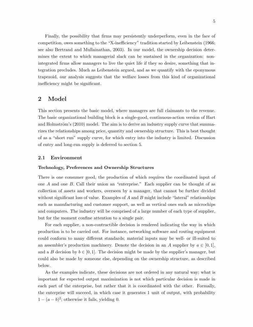
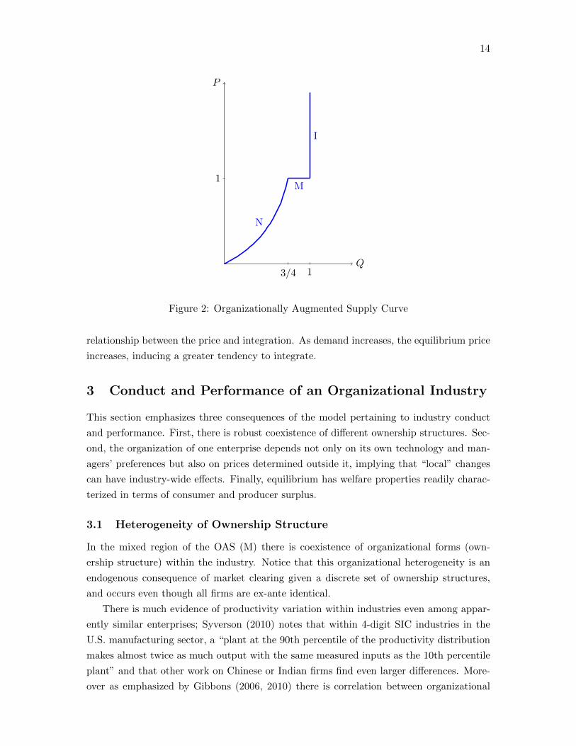
Since supply no longer coincides with marginal cost, it is entirely possible that the

equilibrium will entail inefficiency in the generation of consumer surplus. If the equilibrium

price is below 1/γ, there may be too little integration from the consumer (and shareholder)

point of view, even taking account of the managers’ costs.

0Q

P

QN (γP )

Supply(γ)

1/γ

1

d

d

c′(Q)

ODWL

3/4 1

Figure 3: Ownership Inefficiency when Managers have a Partial Claim on Revenues

An example is illustrated in Figure 3, where the trapezoidal shaded area is the welfare

loss due to organizational inefficiencies when γ < 1. While figure 3 is illustrative, it is

also clear that as the demand function rotates clockwise around the equilibrium price to

become flatter, the deadweight loss is larger, suggesting that demand elasticity plays a role

in determining the magnitude of the welfare loss. We confirm these observations in the

following proposition.

Proposition 4. Suppose that managers are not full revenue claimants (γ < 1).

(a) There is an interval (P (γ)), 1/γ), with P (γ) continuously increasing to P (1) = 1 such

that the equilibrium is ownership inefficient if, and only if, the equilibrium price lies in

16Section5 provides a summary discussion of how the presence of active shareholders, who choose onlythe revenue share optimally, has little impact on the results, whereas if they choose ownership structure aswell, they are apt to integrate too often.

20

this interval.

(b) Consider two demand functions with one more elastic than the other at any price. If

both demands generate the same equilibrium price in (P (γ)), 1/γ)), the organizational

welfare loss is larger for the more elastic demand.

The result that high demand elasticity maximizes welfare losses stands in sharp contrast

to the theory of monopoly with neoclassical firms: there, higher demand elasticities lead

to lower welfare losses. This is one example of how organizational distortions may differ

systematically from market power distortions.

4 Empirical Illustrations: Airlines and Concrete

Recently two studies of very different industries (Forbes and Lederman, 2009, 2010; and

Hortacsu and Syverson, 2007) have provided some evidence that both support our model

and provide an opportunity at explanation. Roughly speaking, the evidence on airlines

correspond to movement along the OAS, while the concrete industry evidence corresponds

to movements of the OAS.

4.1 Airlines

Forbes and Lederman (2009, 2010) describe the relationships between major airlines and

regional carriers. The majors subcontract with the regionals to operate the relatively short

flights that are sold as major carrier flights. In some cases, the major and the regional

are separate firms, in others the regional is owned by the major. Given the hub-and-spoke

design of airline networks, the good required by anyone not living in a hub and needing

to travel to another non-hub must consist of at least two complementary parts, the main

carrier flight and the regional carrier flight, which corresponds rather closely to the situation

we model. There is integration if the major carrier owns the regional carrier.

Forbes and Lederman note that there is heterogeneity of ownership structures: a major

may own some of its regional flights and outsource to others, even on flights originating

out of the same airport. The main issue affecting ownership structure is the flexibility in

adjusting schedules in response to weather or other sources of delay — in other words a

coordination problem where each side is bound to have its own most convenient departure

times. Their data show that integrated relationships perform better (in the sense of fewer

delays and cancellations) and that integration is more likely on routes with more adverse

weather conditions and which are more valuable (routes with more flights or involving more

hubs).

The first result is then consistent with the basic model: the frequency of successful de-

livery of the good is higher under integration than non-integration. More valuable routes

can be interpreted as facing higher demand; then the second result corresponds to a move-

ment along the supply curve: more valuable routes (which would correspond to higher

21

demand functions and therefore higher equilibrium prices) are more likely to be integrated.

That is, airline organization appears to be demand-driven.17

4.2 Cement and Concrete

Hortacsu and Syverson (2007) study the vertical integration levels and productivity of U.S.

cement and ready-mixed concrete producers over several decades and many local markets.

They find that these industries are fairly competitive, that demand is relatively inelastic,

and that there is little evidence that vertical-foreclosure effects of integration are quantita-

tively important. Three of their major findings are (a) prices are lower and quantities are

higher in markets with more integrated firms, (b) high productivity producers are more

likely to be integrated, and (c) some of the more productive firms are non-integrated.

They tie the productivity advantages to improved logistics coordination afforded by large

local concrete operations, regardless of whether it presides in integrated or non-integrated

enterprises.

Though the negative correlation between integration and prices would go against a

single-productivity version of our model, shutting down productivity variation is obviously

a simplification imposed to highlight the importance of demand in determining ownership

structure. The importance of supply-side factors (productivity, complementarity of assets

and investments, and the like) has received the bulk of the emphasis in the literature.

Since as we saw in section 3.2 higher productivity implies integration will occur at

lower price, the Hortacsu-Syverson findings (a) and (b) are explained by assuming there

are multiple (exogenous) productivity levels–markets with more integrated firms are likely

to be those with more productive firms, so equilibrium prices will be lower, assuming equal

demands.

But technological variability alone (and models which exploit this as their only source

of variation in organizational form) cannot fully explain the findings either: if higher

productivity causes integration, why aren’t all productive firms integrated, in contradiction

to finding (c)? Neither supply alone, nor demand alone would seem to be able to explain

the facts of the U.S. concrete and cement industries. But together they can explain the

Hortacsu-Syverson findings.

Suppose, as in section 3.2, that there is exogenous variation in the productivity of

the enterprises in the industry, specifically two productivity levels, 1 and R, with 1 < R.

Demand is isoelastic, with D(P ) = 34P−1. Letting z be the proportion of high productivity

firms, the equilibrium price at z = 0 is P = 1 and all (low productivity) firms are non-

integrated. Now, as z increases in the interval (0, 1) the equilibrium price will decrease

17The result concerning weather can be understood by adding a parameter λ that reflects the loss fromhaving decisions diverge toward the suppliers’ preferred outcomes: the success probability becomes 1 −λ(a − b)2, where large λ corresponds to bad weather. It is straightforward to verify that raising λ makesintegration more likely by lowering the threshold price at which integration occurs. Interestingly, thisimplies that routes with bad weather may actually perform better).

22

from 1 to 1/R.

If the price is strictly larger than 1/R, low productivity firms choose non-integration

while high productivity firms choose integration. If price is equal to 1/R, some of the high

productivity firms will be non-integrated. Either way, high productivity firms are more

likely to be integrated, as in finding (b).

As long as P > 1/R, the proportion of integrated firms is z, and the equilibrium price

solves

zR+ (1− z)QN (P ) =3

4P−1

where the left hand side is the industry supply given the organizational choices of high and

low productivity firms, and the right hand side is the demand. Clearly as z increases in

this region, the equilibrium price must decrease. Thus, consistent with finding (a), price

is negatively correlated with the degree of industry integration. This regime holds as long

as z is smaller than the value z∗ for which the above equality holds with P = 1/R.18

For z > z∗ the equilibrium price ceases to fall and stays at 1/R; at this price managers

in high productivity enterprises are indifferent between integration and non-integration.

Some high productivity firms will have to be non-integrated in order to satisfy the market

clearing condition, while low productivity firms continue to be non-integrated. Hence,

there will be heterogeneity of ownership structure among high productivity enterprises, as

in finding (c).19

The model is flexible enough to provided a unified treatment of the Hortacsu-Syverson

findings in the U.S. ready-mix concrete industry. Of course these patterns are by no

means universal and other relationships between prices and ownership are possible for other

industries, highlighting the importance of demand as well as supply for understanding the

determinants of ownership and its relation to industry performance.

5 Extensions

We now sketch some extensions of the basic model and directions for future research.

5.1 Entry

The model considered so far has a fixed population of price-taking suppliers, correspond-

ing to the standard Arrow-Debreu notion of competition. Industrial economics is also

concerned with ease of entry, which in the present model would also include the choice

18Straightforward computations lead to a cutoff value z∗ = 1 − R/4

R−1+ R2

(R+1)2

. For instance if we take

R = 2, we have z∗ ≈ 65%.19In this region of constant price, it can be shown that the degree of integration will actually fall with z;

but this does not invalidate the non-positive correlation of industry price and degree of integration.

23

of “side” (A or B). Since managers (particularly B’s) earn rents, it is fair to ask what

happens if these rents could be competed away.

Consider the following simple model of entry. There is an unlimited population of ex-

ante identical potential entrants, each of whom receives zero outside the industry and can

choose to become an A or a B. If nA and nB are the measures of people choosing A and

B respectively, the cost of entry borne by an individual entrant is eA(n) = e(nA), eB(n) =

βe(nB) where e(·) is a non-decreasing function.20 The idea is that one side takes a larger

investment than the other (e.g., production requires a larger investment than marketing),

unless β = 1, but that resources devoted to training for either side become scarce as the

industry expands.

A (long-run) equilibrium will consist of measures nA and nB of entrants on each side; a

market clearing product price P and quantity D(P ); and payoffs uA and uB to each of the

entrants, according to which side they take. In equilibrium agents are indifferent between

the two occupations and markets clear; this requires in particular that nA = nB. The scale

(measure of A−B pairs) of the industry will be the common value n. In the product market,

supply embodies ownership choice, as before; following Proposition 1 the integration/non-

integration decisions, and therefore industry output, are determined jointly by |uA − uB|and P. The supply of the industry is nS(|uA−uB|, P ) where S(|uA−uB|, P ) is the output

generated by a unit measure of enterprises, as described in Proposition 1, and n equates

supply and demand.

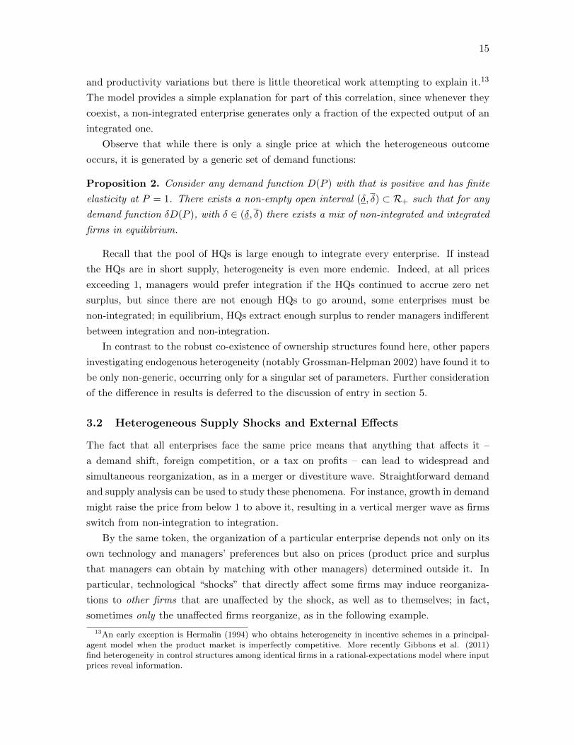
If e(·) is strictly increasing, since agents must be indifferent between the two sides, we

have a payoff expansion path uB = βuA. At low enough prices, this path lies in the non-

integration region |uA − uB| < P1+P . As price increases, the measure n of A’s and B’s, also

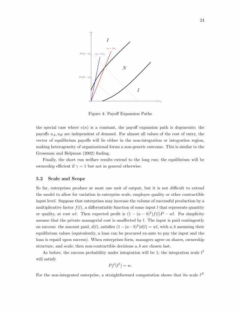
increases, as do the payoffs. Unless β = 1, eventually the payoff expansion path crosses

the |uA − uB| = P1+P loci at a price P ∗(β) and there is a switch to integration. Notice that

a higher value of β means more inequality in the distribution of surplus and since P ∗(β)

is decreasing in β is a force for integration; see figure 4. This echoes our remark following

Proposition 1.

As in the standard neoclassical case, the long run supply will be more price elastic than

the short run supply. Indeed, when P is less than P ∗(β), enterprises are non-integrated

and produce QN (P ), increasing in P . Total managerial welfare must be equal to the total

cost of entry (1 +β)e(n) and therefore since welfare is increasing in P , the number of firms

must also increase with P . The same reasoning holds when P is greater than P ∗(β).

At P = P ∗(β),where managers are indifferent between integration and non-integration,

the quantity supplied will depend on the fraction of integrated enterprises but their number

is fixed. Thus, as in the short run, the supply curve has a horizontal segment at P ∗(β)

and there is generic heterogeneity of organizational forms in a free entry equilibrium. In

20Our baseline model is equivalent to having a fixed supply of B and A suppliers having an exogenousoutside option of e(1). That is, the A suppliers (and HQ’s) are mobile while the B suppliers are not. Thelong run analysis also makes the Bs mobile.

24

0

uB

uA

N

I

I

uB = βuA

uB = β′uAP ∗(β)− 1/2

P ∗(β′)− 1/2

Figure 4: Payoff Expansion Paths

the special case where e(n) is a constant, the payoff expansion path is degenerate; the

payoffs uA, uB are independent of demand. For almost all values of the cost of entry, the

vector of equilibrium payoffs will lie either in the non-integration or integration region,

making heterogeneity of organizational forms a non-generic outcome. This is similar to the

Grossman and Helpman (2002) finding.

Finally, the short run welfare results extend to the long run; the equilibrium will be

ownership efficient if γ = 1 but not in general otherwise.

5.2 Scale and Scope

So far, enterprises produce at most one unit of output, but it is not difficult to extend

the model to allow for variation in enterprise scale, employee quality or other contractible

input level. Suppose that enterprises may increase the volume of successful production by a

multiplicative factor f(l), a differentiable function of some input l that represents quantity

or quality, at cost wl. Then expected profit is (1 − (a − b)2)f(l)P − wl. For simplicity

assume that the private managerial cost is unaffected by l. The input is paid contingently

on success: the amount paid, d(l), satisfies (1− (a− b)2)d(l) = wl, with a, b assuming their

equilibrium values (equivalently, a loan can be procured ex-ante to pay the input and the

loan is repaid upon success). When enterprises form, managers agree on shares, ownership

structure, and scale; then non-contractible decisions a, b are chosen last.

As before, the success probability under integration will be 1; the integration scale lI

will satisfy

Pf ′(lI) = w.

For the non-integrated enterprise, a straightforward computation shows that its scale lN

25

satisfies

QPf ′(lN ) = w,

where Q = QN (Pf(lN )− d(lN )). Thus marginal returns to l are greater under integration.

From Topkis’s theorem, lI > lN . And as before, there will be a price at which managers

are indifferent between integration and non-integration.

Hence, when they coexist, integrated firms are both bigger and “smarter” (in the al-

ternative interpretation of l as quality) than non-integrated ones.21 Therefore the output

gap between the two kinds of enterprises is amplified. Whether these endogenous output

differences could explain the large productivity differences that observed in many industries

is left for further research.

Another extension of the model involves the analysis of firm scope, wherein each supplier

produces its own distinct good for sale on the market, as in the original Hart-Holmstrom

model. Because it involves strategic interactions among different parts of the enterprise,

this is somewhat intricate, particularly if the number of suppliers is greater than two.

Legros and Newman (2012) considers such a model. As here integration yields coordination

but at a high cost for the managers of individual product lines. Moreover, an integrated

firm provides coordination benefits not only to its members, but also for “outsiders,” who

can can free ride. The integrated firm is typically tempted to follow the preferences of

the outsiders, who therefore enjoy coordination benefits at lower cost than insiders. This

mechanism provides a limit to the extent of integration, and the paper shows that the scope

of multi-product firms depends on both the mean and the variance of individual product

prices.

5.3 Finance

The responsiveness of ownership choice to industrial conditions in the model emerges in

large measure because managers have finite (in fact, zero) wealth. This assumption implies

that the ownership structure is dependent on the distribution of surplus between them,

and that in turn leads to the relationship between industry price and degree of integration

embedded in the OAS. It is worth devoting some attention to the comparative statics of

the wealth endowments, as this appears to be connected more generally to the role that

financial contracting would have in affecting industry performance.

One important difference between integration and non-integration is the degree of trans-

ferability in managerial surplus: while managerial welfare can be transferred 1 to 1 with

integration (that is one more unit of surplus given to B costs one unit of surplus to A), this

is no longer true with non-integration. If the A manager has cash that can be transferred

without loss to the B managers before production takes place, the advantage of integration

in terms of transferability is reduced. This has immediate consequences for the OAS.

21This result persists if managerial costs are a function of the scale as long as these costs do not growtoo quickly with respect to l. Details available upon request.

26

Proposition 5. Positive shocks to the cash endowments of suppliers A decrease the level

of integration and shift the OAS to the left.

The observation that positive shocks to the cash endowments of suppliers A decrease the

level of integration implies in particular that if managers have access to infinite amounts of

cash, they will always contract for equal sharing in non-integrated organizations. However,

for any finite cash holdings, there is a level of price high enough for which there will be

integration.

These observations apply with equal force when the managers are not full residual

claimants on the revenues of the firm. Since integration is output maximizing, inefficiencies

increase from the point of view of consumers and shareholders. Thus, in contrast to previous

literature that has suggested that managerial cash holdings may lead to firms are too large,

this model suggests it may generate firms that are too small.22

Finite endowments is not incompatible with a well functioning financial market, and this

raises the question of whether borrowing for lump-sum payments would change contracting.

Because there is full transferability under integration, debt could have a limited role in

allowing HQ to ‘buy the firm” and, as we have discussed, will not affect output as long

as HQ has a positive share of output. By contrast under non-integration, if a debt D

has to be repaid in case of success, managers effectively face a revenue of P − D, and

output will decrease from QN (P ) to QN (P −D); this leads to a decrease in total welfare

unless this decrease from UN (P ) to UN (P −D) is compensated by the ex-ante lump-sum

QN (P −D)D. If uA = 0, as we have assumed in most of the paper, this cannot be the case

and managers will never use debt to finance lump-sum transfers under non-integration.23

When uA is positive however, there is a range of prices for which small amounts of debt

for side-payments may raise managerial welfare, enlarging the set of prices for which non-

integration is chosen. However debt unambiguously reduces output in this case; hence

leveraged non-integrated firms lower consumer surplus. A more general analysis is available

in Legros and Newman (2012).

Proposition 6. Suppose that uA = 0. Non-integrated firms do not use debt for ex-ante

side-payments. HQ may use debt to finance the purchase of assets.

Note that debt is here used only to finance ex-ante side payments and not acquisition

of assets from outside the relationship. If firms have investment opportunities, e.g., to

expand their scale of production, non-integrated firms are at a disadvantage for borrowing

since debt has a depressing effect on expected output.

22As in Jensen (1986) managers will tend to use cash for their own interest rather than that of shareholdersor consumers but while in the free cash flow theory they will tend to use cash for “empire building” orover-expansion, here they use cash to keep firms small and buy a “quiet life”.

23This is because when uA = 0, A’s choice is independent of revenue and the non-integration gamereduces to a single decision maker B. Since at price P , B chooses optimally a level of output of QN (P ), hewill choose D = 0 in order to maximize his total payoff of QN (P −D)P − c(QN (P −D)).

27

Active Shareholders

In our model, managers have control over the integration decisions and ownership ineffi-

ciencies take the form of too little integration. Since shareholders have similar objectives

as consumers — they value high output — a reasonable conjecture is that efficiency may

be improved when shareholders have control over integration decisions and compensation

to managers. Corporate governance is now relevant not only for shareholders but also for

consumers.

Providing good incentives is costly to shareholders under non-integration, since it entails

giving up a share of profit to management, and that cost is fairly sensitive to P . By

contrast, integration has the benefit of providing full coordination, while its cost (1/2)

will be independent of the price. Hence, if shareholders have control over organizational

choices and compensation schemes, non-integration will underperform relative to the social

optimum.

Recall that integration is ownership efficient for prices above the value of P for which

P − 1/2 = UN (P ). Shareholders will choose γ < 1 to maximize their expected revenue(1− 1

(1+γP )

)2(1 − γ)P . The maximized value is increasing convex and is everywhere

smaller than the minimum value of UN (P ), which is P 2

1+P . It follows that shareholders will

choose integration at prices below the efficient level.

Proposition 7. Suppose that the shareholders control the decision to integrate and the

shares of output going to the two managers. The minimum price at which shareholders

choose integration is strictly lower than the ownership efficient level.

Shareholder control could therefore substitute for the planner’s forced integration as

a means of protecting consumers, but this can be taken too far. The policy question of

how to regulate governance when consumers are affected by firm’s organizational choices is

an open question. The literature on corporate governance tends to emphasize high profit

regimes as most conducive to managerial cheating, presumably because high profit regimes

are most conducive to “profit taking,” like diversion of revenues to private managerial

benefits or investments in pet projects. But as we have seen, governance also matters for

“profit making”: proper organizational design affects managers’ production decisions, and

is particularly important when low profitability provides weak incentives for them to invest

in a profit or output maximizing way.

6 Conclusion

Industrial economics has focused almost exclusively on strategic and collusive interactions

among firms in imperfectly competitive markets. But, as we have shown, it is not only

industrial structure but also organization that is an important determinant of conduct

28

and performance. In fact, conduct may be dictated directly by organizational choices and,

reciprocally, organizational choices will be guided by market conditions.

Organization theory benefits IO because it can help explain heterogeneity in firm per-

formance, shows that industry performance is dependent on organizational design, and

suggests that such topics as the diffusion of innovation may be affected by organizational

choices.

On the other hand, IO helps organization economics. Market forces help determine

organization choices. Other underlying models of integration may generate other relation-

ships among prices, quantities and integration: that is the OAS may have different shapes

for different theories. One benefit of unifying organizational and industrial economics is

that market data become the proving ground for different organizational theories, includ-

ing those that might predict a negative or non-monotonic relationship between price and

integration.

Our model is based on one important tradeoff between non-integration and integration:

non-integration is strong on internalizing private costs and weak on coordinating decisions;

integration has the opposite strength and weakness. Its predictions are consistent with a

number of empirical findings in the cement and airlines industries.

The analysis shows that consumers have an interest in the organization of the firms

that make the products they buy. An influential strand of thought asserts that competition

in the product market must assure efficient outcomes: firms that do not deliver the goods

at the lowest feasible cost, whatever the reason, including inefficient organization, will be

supplanted by ones that do.24 The present framework confronts such claims directly by

embedding organizational firms into perfectly competitive settings. While efficient owner-

ship may prevail when managers have full title to enterprise revenue, in the general case,

organizational choices may not be ownership efficient. Monopoly need not be the only

refuge for a quiet life.

Finally, while the model goes some way toward the organizational IO objective of jointly

determining market structure, performance and ownership structures, much remains to be

done. In particular, rather than assuming perfect competition, we would want to consider

environments where market power would play a role so that the degree of competition

would be endogenous.

A Appendix: Proofs

Proofs of the Results in Section 3.3

The results in the text are stated in the context of zero outside options for the A managers,

we prove below that these results hold for any level of outside option.

24The “form of organization that survives... is the one that delivers the product demanded by customersat the lowest price while covering costs.” (Fama and Jensen, 1983).

29

With non-integration, in order to meet his outside option, A must get a share s(P ;uA)

solving

uNA (s, P ) = uA.

Defining α(s) ≡ s2 + (1− s)2, UN (s, P ) in (5) can be written as:

UN (s, P ) = QN (P )P − α(s)

(P

1 + P

)2

.

Therefore the maximum payoff to B when the outside option of A is is uA is equal to

UN (s(P ;uA), P )− uA. (A.1)

Finally, the cost under non-integration is

CN (QN (γP );uA) = α(s(γP ;uA))c(QN (γP )).

Proof of Proposition 3

Suppose that demand is perfectly elastic. With integration, B gets P − 12 −uA, while with

non-integration he gets uNB (s(P ;uA), P ) = UN (s(P ;uA), P ) − uA. It follows B manager

chooses an organization if, and only if, the total managerial welfare is greater. Because

when demand is perfectly elastic the total welfare coincides with the total managerial

welfare, the result follows.

With a less elastic demand, let PN be the equilibrium price under non-integration. If

firms are forced to integrate, industry supply increases and therefore the new equilibrium

is P I < PN since demand is decreasing. The difference in total welfare between forced

integration at price P I and non-integration at price PN is bounded above by U I(PN ) −UN (PN ), which is negative by the previous argument. Hence the initial equilibrium is

ownership efficient.

Proof of Proposition 4

We first consider the welfare of shareholders and managers: this coincides with the to-

tal welfare when the demand is perfectly elastic. We will then consider general demand

functions.

Perfectly Elastic Demand. Let us define the sum of the welfares of shareholders and

managers when γ is less than 1 by,

V N (P, γ) = (1− γ)QN (γP )P + UN (s(γP ;uA), γP ),

V I(P ) = P − 1/2

30

Furthermore, let P ∗(uA) be the unique value solving UN (s(P ;uA), P ) = U I(P ).

Lemma A.1. Suppose that shareholders receive a share 1−γ > 0 of the firm’s revenue and

that the outside option of A managers is uA. Then there exist p(γ) < P ∗(uA)/γ such that

equilibria with P ∈ (p(γ), P ∗(uA)/γ) are such that V N (P, γ) < V I(P, γ).

Proof. From Proposition 1, non-integration is chosen if and only if the price is less than

P ∗(uA)/γ. For this price, the managers act as if they faced a revenue of P ∗(uA) and

therefore will choose to produce QN (P ∗(uA)) under non-integration.

V N (P ∗(uA)/γ, γ) = (1− γ)P ∗(uA)

γQN (P ∗(uA)) + UN (s(P ∗(uA);uA), P ∗(uA))

= (1− γ)P ∗(uA)

γQN (P ∗(uA)) + P ∗(uA)− 1/2

<P ∗(uA)

γ− 1/2

= V I(P ∗(uA)/γ)

where the strict inequality followsQN (P ∗(uA)) < 1. Now, since the functions V N (P, γ), V I(P )

are continuous in P , there exists p(γ) with the desired property and proves the lemma.

Letting ω(P ) be the consumer surplus at price P , total welfare under laissez-faire is

then ω(P ) +α(P ))V I(P, γ) + (1−α(P )V N (P, γ), here α(P ) is the equilibrium measure of

integrated firms (see section 2.4.)

For perfectly elastic demand functions, ω(P ) ≡ 0 and therefore total welfare coincides

with α(P ))V I(P, γ) + (1−α(P )V N (P, γ) implying that equilibria are ownership inefficient

for all prices in the interval described in lemma A.1.

Arbitrary Demand Functions. Consider an arbitrary demand function and let ω(P )

be the consumer surplus associated to this demand function. Since utility is quasi-linear:

ω′(P ) = −D(P ). (A.2)

Let us denote by εD(P ), εS(P ) the price elasticities of demand and of supply. Suppose

that the equilibrium is achieved at a price P in the interval (p(γ), P ∗(uA)/γ] of Lemma

A.1.

We write the total welfare when the price is P and the proportion of firms that integrate

is α as:25

W (P, α) ≡ ω(P ) + αV I(P, γ) + (1− α)V N (P, γ). (A.3)

25Under laissez-faire, we have α = α(P ) but this is not the case under planner’s intervention.

31

As P < P ∗(uA)/γ, firms choose non-integration with probability one. Therefore total

welfare at this equilibrium is W (P, 0) = ω(P ) + V N (P, γ) while we know that V N (P, γ) <

V I(P, γ) by lemma A.1. We consider a thought experiment where the planner forces a

small proportion α of firms to integrate; the firms that are free to choose their organization

continue to choose non-integration and therefore the total supply in the industry is α +

(1−α)QN (γP ) if the price is P . However because total supply increases after the planner’s

intervention, the new equilibrium on the market is at price pe(α) < P satisfying:

D(pe(α)) = α+ (1− α)QN (γpe(α)). (A.4)

The welfare after the planner’s intervention is now:

W (pe(α), α) = ω(pe(α)) + αV I(pe(α), γ) + (1− α)V N (pe(α), γ).

Implicitly differentiating (A.4) and using (A.2) we compute dW (pe(0), 0)/dα by taking

the limit of dW (pe(α), α)/dα as α converges to 0; dW (pe(0), 0)/dα therefore captures the

local benefit of forcing firms to integrate. After straightforward computations we have

dW (pe(0), 0)/dα > 0 if, and only if:

(1− γ)εS(γP )

εS(γP ) + |εD(P )|<V I(P, γ)− V N (P, γ)

1−QN (γP ). (A.5)

If the demand function is perfectly elastic, the right hand side of (A.5) is the average

welfare gain when all firms are forced to integrate. The left hand side is the welfare loss

for the 1− γ non-integrated firms due to the decrease in price.

As |εD| → ∞, the left hand side goes to zero and we recover the condition of lemma

A.1. As |εD| decreases, the left hand side increases and therefore the condition is harder

to satisfy at a given equilibrium price P , proving the proposition.

As a matter of illustration, consider the case uA = 0 and a demand function such that

the equilibrium price is 1/γ and the equilibrium quantity is QN (1) = 3/4. in this case,

εS(1) = 1/3 and the condition reduces to γ < 1 + 3|εD| which is always satisfied. Hence,

the condition holds indeed strictly at P = 1/γ, and therefore the range of prices for which

there is local ownership inefficiency is a non-trivial subset of the interval (PN (γ), 1/γ] of

Lemma A.1.

Proof of Proposition 5

Under non-integration, cash is a more efficient instrument for surplus allocation than the

sharing rule s between managers A and B since a change of s affects total costs. By

contrast, when firms are integrated, a change in s has no effect on output or costs and

therefore shares are as efficient at allocating surplus as cash. Hence, introducing managerial

cash endowments favors non-integration, and we would observe fewer integrated firms.

32

Let us return to our baseline environment where the population of B’s is fixed and

uA = 0. Assume for simplicity that all A managers have the same cash holding of `.

A contract now specifies a lump sum transfer t from the A manager to the B manager

together with a share s of output and an organization. Because the managerial surplus

is transferable under integration, cash transfers are neutral. For non-integration however,

since the total surplus is increasing on s ∈ [0, 1/2], the ability for the A managers to make

cash transfers in exchange for a greater share of output will increase managerial surplus.

Final payoffs are then uNA (s, P )− t and uNB (s, P ) + t, where uNA , uNB are given by (3).

By competition, the marginal manager A must have a zero surplus. For a given market

price P , if ` > UN (1/2, P ), A managers are able to transfer t = UN (1/2, P )/2 to the B

manager at the signing of the contract in exchange for a share of 1/2 of the output. In this

case, the payoff to the B managers is UN (1/2, P ). If ` < UN (1/2, P ), the A manager uses a

transfer t = ` in exchange for a share s`(P ) of the revenue satisfying:

uNA (s`(P ), P ) = `.

In this case, managers B have, after the transfer of t = `, a payoff of:

uNB (s`(P ), P ) + ` = UN (s`(P ), P ).

While there is a larger managerial surplus, the output under non-integration is the same

as before. Because non-integration is now more efficient from the point of view of manager

B, integration will be chosen for a price greater than 1.26 Indeed, as ` increases, s`(P )

increases, therefore welfare under non-integration increases, and the shift to integration

happens at higher prices.

Proof of Proposition 6

Debt and Non-Integration. Because of full transferability, debt has no incentive effects

for integration. This is not the case with non-integration. Note first that cash transfers

are not the same as monetary transfers made after borrowing: an ex-ante transfer does not

affect managers’ incentives but the ex-post repayment of debt will weaken the incentives

of the borrower since the value of coordination is lower than without debt. For instance

suppose that manager A borrows t in exchange of a repayment of D = t/Q∗ where Q∗ is

the anticipated probability of success.

There is no loss of generality in assuming that the manager B is fully liable for the debt

and gives a zero share to A.27 The probability of success is QN (P −D) and therefore debt

26Total managerial welfare under non-integration can be written as UN (s`(P ), P ) = PQN (P ) −β(s`(P ))c(QN (P )) with β(s) ≡ s2 + (1 − s)2 Since β(s) is a decreasing function of s ∈ [0, 1/2], totalmanagerial welfare increases in s. By contrast, managerial welfare under integration is UI(P ) = P − 1/2which is independent of `.

27Indeed, if the contract has A liable for the debt, A must have a share of s such that sP ≥ D and

33

can finance an ex-ante transfer of QN (P −D)D. It follows that the ex-ante expected payoff

of manager B when there is borrowing is equal to QN (P−D)P−c(QN (P−D)). By revealed

preferences, the maximum welfare to B when s = 0 is attained at QN (P )P − c(QN (P )),

and therefore the maximum of QN (P −D)P − c(QN (P −D)) is obtained at D = 0. Hence,

manager A will not use debt to make lump-sum payments to manager B, as claimed.

Debt and Integration. Contrary to non-integration, debt may have value when there

is integration. We know from section 2.3 that HQ must have a strictly positive share of

the firm’s revenue, and that there is no loss of generality in assuming that this stake is

100%. The maximum ex-ante transfer she is willing to make to the managers is P . If her

cash endowment is positive (however small), she can always finance the rest of the asset

purchase with debt since debt has no distortionary effects on her incentives. Indeed, if she

owes D, her interim payoff is (1 − (a − b)2)(P − D), which still results in a = b = 1/2,

provided D < P .

If however she is fully leveraged, with D = P , then neither she nor the managers have a

positive stake in the revenue, and ex-post they would all agree to implement (a, b) = (1, 0)

in order to minimize costs! Anticipating this, a lender would refuse a loan. It follows that

HQ’s must finance their acquisitions partly with cash.

References

[1] Aghion, Philippe and Jean Tirole (1994), “The Management of Innovation,” The

Quarterly Journal of Economics, 109: 1185-1209.

[2] Alonso, Roberto, Dessein, Wouter and Matouschek, Niko (2008): “Centralization Ver-

sus Decentralization: An Application to Price Setting By a Multi-Market Firm,” Jour-

nal of the European Economic Association, 6: 457-67.

[3] Antras, Paul and Helpman, Elhanan. (2004), “Global Sourcing,” Journal of Political

Economy, 112: 552-80.

[4] Antras, Paul (2003), “Firms, Contacts, and Trade Structure,” Quarterly Journal of

Economics, 118: 1357-418.

[5] Bertrand, Marianne and Sendhil Mullainathan (2003), “Enjoying the Quiet Life? Cor-

porate Governance and Managerial Preferences,” Journal of Political Economy, 111:

1043-1075.

the payoffs to the two managers are respectively uA = (1 − (a − b)2)(sP − D) − (1 − a)2 and uB =(1 − (a − b)2)(1 − s)P − b2. By making the change of variable s = (sP −D)/(P −D), the payoffs can bewritten as uA = (1− (a− b)2)s(P −D)− (1− a)2 and uB = (1− (a− b)2)(1− s)(P −D)− b2, implying thesame equilibrium for a, b as in the initial contract. The problem is then equivalent to our baseline model ofnon-integration with a price equal to P −D where each of A and B are responsible for the debt repayment.It is then optimal for manager B to set s = 0, hence B wants indeed to be fully responsible for the debtrepayment.

34

[6] Brander, James A., and Tracy R. Lewis (1986), “Oligopoly and Financial Structure:

The Limited Liability Effect.” The American Economic Review, 76: 956970.

[7] Chamberlin, Edward (1933). Theory of Monopolistic Competition. Cambridge, MA:

Harvard University Press.

[8] Conconi, Paola, Patrick Legros and Andrew Newman (forthcoming), “Trade Liberal-

ization and Organizational Change,” Journal of International Economics.

[9] Fama, Eugene F., and Michael C. Jensen (1983), “Separation of Ownership and Con-

trol,” Journal of Law and Economics, 26: 301-325.

[10] Fershtman, Chaim, and Kenneth L Judd (1987), “Equilibrium Incentives in

Oligopoly,” American Economic Review 77: 927940.

[11] Forbes, Silke J., and Mara Lederman (2009), Adaptation and Vertical Integration in

the Airline Industry. American Economic Review 99: 18311849.

[12] (2010), Does vertical integration affect firm performance? evidence from the

airline industry. The RAND Journal of Economics 41: 765-790.

[13] Gibbons, Robert (2006), “What the Folk Theorem doesn’t tell us,” Industrial and

Corporate Change, 15: 381-386.

[14] (2010), “Inside Organizations: Pricing, Politics, and Path Dependence,” An-

nual Review of Economics, 2: 337-365.

[15] Gibbons, Robert, Richard Holden and Michael Powell (2011), “Organization and Infor-

mation: Firm’s Governance Choices in Rational Expectations Equilibrium,” working

paper, MIT.

[16] Grossman, Sanford and Oliver Hart (1986), “The Costs and Benefits of Ownership:

A Theory of Vertical and Lateral integration,” Journal of Political Economy, 94: 691-

719.

[17] Grossman, Gene M. and Helpman, Elhanan (2002), “Integration Versus Outsourcing

in Industry Equilibrium,” The Quarterly Journal of Economics, 117: 85-120.

[18] Hart, Oliver (1983), “The Market Mechanism as an Incentive Scheme” Bell Journal

of Economics , 14: 366-382.

[19] Hart, Oliver and Bengt Holmstrom (2010), “A Theory of Firm Scope,” The Quarterly

Journal of Economics, 125: 483-513.

[20] Hart, Oliver and John Moore (1990), “Property Rights and the Nature of the Firm,”

Journal of Political Economy, 98: 1119-1158.

35

[21] Hermalin, Benjamin E. (1992), “Heterogeneity in Organizational Form: Why Other-

wise Identical Firms Choose Different Incentives for Their Managers?” The RAND

Journal of Economics, 25, 518-34.

[22] Hortacsu, Ali, and Chad Syverson (2007), “ Cementing Relationships: Vertical In-

tegration, Foreclosure, Productivity, and Prices,” Journal of Political Economy, 113:

250-301.

[23] Jensen, Michael C. (1986), “Agency Cost of Free Cash Flow, Corporate Finance, and

Takeovers,” American Economic Review, 76:323-329.

[24] Legros, Patrick and Andrew F. Newman (1996), “Wealth Effects, Distribution and

the Theory of Organization” Journal of Economic Theory, 70: 312-41.

[25] (2008), “Competing for Ownership,” Journal of the European Economic As-

sociation, 6: 1279-1308.

[26] (2009), “A Price Theory of Vertical and Lateral Integration,” CEPR WP

7211, March.

[27] (2010), “A Price Theory of Firm Scope,” mimeo, ECARES, April.

[28] (2011), “On the Impossibility of Disinterested Authority, with Applications

to CEO Pay” mimeo ECARES and BU, December.

[29] (2012), “Debt and Efficient Contracting in Partnerships” mimeo, ECARES

and BU, January.

[30] Leibenstein, Harvey (1966), “Allocative Efficiency Vs. ‘X-efficiency”’American Eco-

nomic Review, 56: 392-415.

[31] Machlup, Fritz (1967), “Theories of the Firm: Marginalist, Managerial, Behavioral,”

American Economic Review, 57: 1-33.

[32] Marin, Dalia and Verdier, Thierry (2008), “Power Inside the Firm and the Market: A

General Equilibrium Approach,” Journal of the European Economic Association, 6:

752-88.

[33] Mclaren, John (2000) “Globalization and Vertical Structure,” The American Economic

Review, 90: 1239-54.

[34] Raith, Michael (2003), “Competition, Risk, and Managerial Incentives,” The Ameri-

can Economic Review 93: 14251436.

[35] Schmidt, Klaus (1997), “Managerial Incentives and Product Market Competition”,

Review of Economic Studies 64: 191-214.

36

[36] Scharfstein, David (1988), “Product-Market Competition and Managerial The RAND

Journal of Economics 19: 147155.

[37] Syverson, Chad (2010), “What determines productivity?” working paper, U. of

Chicago.

[38] van den Steen, Eric (2005), “ Organizational beliefs and managerial vision,” Journal

of Law, Economics, and Organization, 21: 256-283.

[39] Whinston, Michael D. (2001), “Assessing the Property Rights and Transaction-Cost

Theories of Firm Scope,” The American Economic Review, Papers and Proceedings

of the Hundred Thirteenth Annual Meeting of the American Economic Association,

91: 184-188.