Embed Size (px)
Citation preview
Source URL: http://numericalmethods.eng.usf.edu/ Saylor URL: http://www.saylor.org/courses/me205/
Attributed to: University of South Florida: Holistic Numerical Methods Institute Saylor.org
Page 1 of 39
Primer for Ordinary Differential Equations Autar Kaw
After reading this chapter, you should be able to:
1. define an ordinary differential equation, 2. differentiate between an ordinary and partial differential equation, and 3. solve linear ordinary differential equations with fixed constants by using classical
solution and Laplace transform techniques.
Introduction
An equation that consists of derivatives is called a differential equation. Differential
equations have applications in all areas of science and engineering. Mathematical
formulation of most of the physical and engineering problems leads to differential
equations. So, it is important for engineers and scientists to know how to set up
differential equations and solve them.
Differential equations are of two types
(A) ordinary differential equations (ODE) (B) partial differential equations (PDE)
An ordinary differential equation is that in which all the derivatives are with respect to a
single independent variable. Examples of ordinary differential equations include
022
2
=++ ydx
dy
dx
yd, 4)0( ,2)0( == ydx
dy,
,sin532
2
3
3
xydx
dy
dx
yd
dx
yd=+++ ,12)0(
2
2
=dx
yd 2)0( =dx
dy, 4)0( =y
Ordinary differential equations are classified in terms of order and degree. Order of an
ordinary differential equation is the same as the highest derivative and the degree of an
ordinary differential equation is the power of highest derivative.
Source URL: http://numericalmethods.eng.usf.edu/ Saylor URL: http://www.saylor.org/courses/me205/
Attributed to: University of South Florida: Holistic Numerical Methods Institute Saylor.org
Page 2 of 39
Thus the differential equation,
xexydx
dyx
dx
ydx
dx
ydx =+++
2
22
3
33
is of order 3 and degree 1, whereas the differential equation
xdx
dyx
dx
dysin1 2
2
=+
+
is of order 1 and degree 2.
An engineer’s approach to differential equations is different from a mathematician.
While, the latter is interested in the mathematical solution, an engineer should be able
to interpret the result physically. So, an engineer’s approach can be divided into three
phases:
a) formulation of a differential equation from a given physical situation, b) solving the differential equation and evaluating the constants, using given
conditions, and c) interpreting the results physically for implementation.
Formulation of differential equations
As discussed above, the formulation of a differential equation is based on a given
physical situation. This can be illustrated by a spring-mass-damper system.
Source URL: http://numericalmethods.eng.usf.edu/ Saylor URL: http://www.saylor.org/courses/me205/
Attributed to: University of South Florida: Holistic Numerical Methods Institute Saylor.org
Page 3 of 39
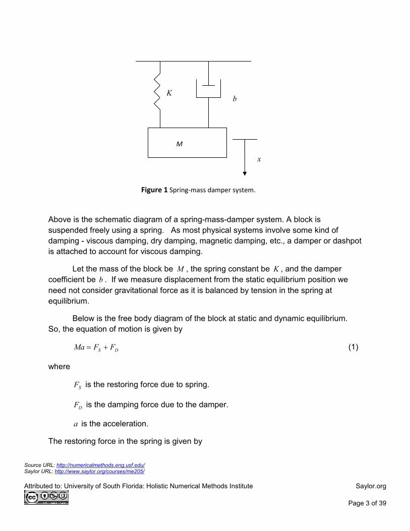
Above is the schematic diagram of a spring-mass-damper system. A block is
suspended freely using a spring. As most physical systems involve some kind of
damping - viscous damping, dry damping, magnetic damping, etc., a damper or dashpot
is attached to account for viscous damping.
Let the mass of the block be M , the spring constant be K , and the damper
coefficient be b . If we measure displacement from the static equilibrium position we
need not consider gravitational force as it is balanced by tension in the spring at
equilibrium.
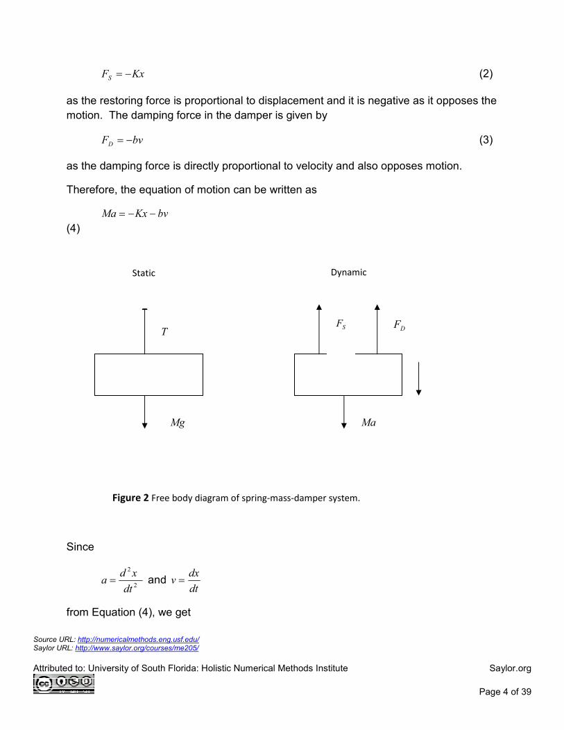
Below is the free body diagram of the block at static and dynamic equilibrium.
So, the equation of motion is given by
DS FFMa += (1)
where
SF is the restoring force due to spring.
DF is the damping force due to the damper.
a is the acceleration.
The restoring force in the spring is given by
K b
x
Figure 1 Spring-mass damper system.
M
Source URL: http://numericalmethods.eng.usf.edu/ Saylor URL: http://www.saylor.org/courses/me205/
Attributed to: University of South Florida: Holistic Numerical Methods Institute Saylor.org
Page 4 of 39
KxFS −= (2)
as the restoring force is proportional to displacement and it is negative as it opposes the
motion. The damping force in the damper is given by
bvFD −= (3)
as the damping force is directly proportional to velocity and also opposes motion.
Therefore, the equation of motion can be written as
bvKxMa −−=
(4)
Since
2
2
dt
xda = and
dt
dxv =
from Equation (4), we get
SF
Ma
DF
T
Mg
Figure 2 Free body diagram of spring-mass-damper system.
Static Dynamic
Source URL: http://numericalmethods.eng.usf.edu/ Saylor URL: http://www.saylor.org/courses/me205/
Attributed to: University of South Florida: Holistic Numerical Methods Institute Saylor.org
Page 5 of 39
dt
dxbKx
dt
xdM −−=
2
2
02
2
=++ Kxdt
dxb
dt
xdM (5)
This is an ordinary differential equation of second order and of degree one.
Solution to linear ordinary differential equations
In this section we discuss two techniques used to solve ordinary differential equations
(A) Classical technique (B) Laplace transform technique
Classical Technique
The general form of a linear ordinary differential equation with constant coefficients is
given by
)(......... 122
2
31
1
xFykdx
dyk
dx
ydk
dx
ydk
dx
ydn
n
nn
n
=+++++−
−
(6)
The general solution contains two parts
PH yyy += (7)
where
Hy is the homogeneous part of the solution and
Py is the particular part of the solution.
The homogeneous part of the solution Hy is that part of the solution that gives zero
when substituted in the left hand side of the equation. So, Hy is solution of the equation
0......... 122
2
31
1
=+++++−
−
ykdx
dyk
dx
ydk
dx
ydk
dx
ydn
n
nn
n
(8)
Source URL: http://numericalmethods.eng.usf.edu/ Saylor URL: http://www.saylor.org/courses/me205/
Attributed to: University of South Florida: Holistic Numerical Methods Institute Saylor.org
Page 6 of 39
The above equation can be symbolically written as
0................. 12
1 =++++ − ykDykyDkyD n
n
n (9)
0).................( 12
1 =++++ − ykDkDkD n
n
n (10)
where,
n
nn
dx
dD =
(11)
.
.
.
1
11
−
−− =
n
nn
dx
dD
operating on y is the same as
),( 1rD − )( 2rD − , )( nrD −
operating one after the other in any order, where
)(....,),........(),( 21 nrDrDrD −−−
are factors of
0............... 12
1 =++++ − kDkDkD n
n
n (12)
To illustrate
0)23( 2 =+− yDD
is same as
0)1)(2( =−− yDD
0)2)(1( =−− yDD
Source URL: http://numericalmethods.eng.usf.edu/ Saylor URL: http://www.saylor.org/courses/me205/
Attributed to: University of South Florida: Holistic Numerical Methods Institute Saylor.org
Page 7 of 39
Therefore,
0)....................( 12
1 =++++ − ykDkDkD n
n
n (13)
is same as
0).........().........)(( 11 =−−− − yrDrDrD nn (14)
operating one after the other in any order.
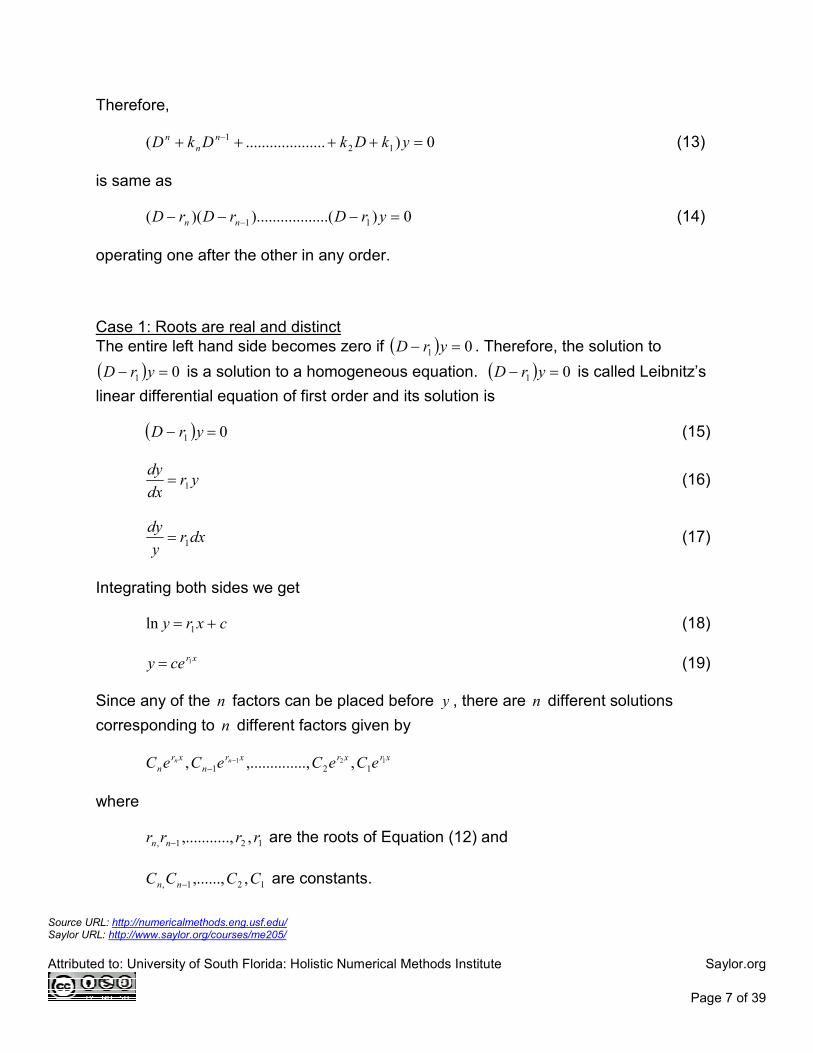
Case 1: Roots are real and distinct
The entire left hand side becomes zero if ( ) 01 =− yrD . Therefore, the solution to
( ) 01 =− yrD is a solution to a homogeneous equation. ( ) 01 =− yrD is called Leibnitz’s
linear differential equation of first order and its solution is
( ) 01 =− yrD (15)
yrdx
dy1= (16)
dxry
dy1= (17)
Integrating both sides we get
cxry += 1ln (18)
xrcey 1= (19)
Since any of the n factors can be placed before y , there are n different solutions
corresponding to n different factors given by
xrxrxr
n
xr
n eCeCeCeC nn 121
121 ,.....,,........., −−
where
121, ,..,,......... rrrr nn − are the roots of Equation (12) and
121, ,,......, CCCC nn − are constants.

Source URL: http://numericalmethods.eng.usf.edu/ Saylor URL: http://www.saylor.org/courses/me205/
Attributed to: University of South Florida: Holistic Numerical Methods Institute Saylor.org
Page 8 of 39
We get the general solution for a homogeneous equation by superimposing the
individual Leibnitz’s solutions. Therefore
xr
n
xr
n
xrxr
Hnn eCeCeCeCy ++++= −
−121
121 ............. (20)
Case 2: Roots are real and identical
If two roots of a homogeneous equation are equal, say 21 rr = , then
0))(...(..........).........)(( 111 =−−−− − yrDrDrDrD nn (21)
Let’s work at
0))(( 11 =−− yrDrD (22)
If
zyrD =− )( 1 (23)
then
0)( 1 =− zrD
xreCz 1
2= (24)
Now substituting the solution from Equation (24) in Equation (23)
xreCyrD 1
21)( =−
xreCyr
dx
dy1
21 =−
2111 Cyer
dx
dye
xrxr =− −−
2
)( 1
Cdx
yedxr
=−
dxCyed xr
2)( 1 =− (25)
Source URL: http://numericalmethods.eng.usf.edu/ Saylor URL: http://www.saylor.org/courses/me205/
Attributed to: University of South Florida: Holistic Numerical Methods Institute Saylor.org
Page 9 of 39
Integrating both sides of Equation (25), we get
121 CxCye xr +=−
xreCxCy 1)( 12 += (26)
Therefore the final homogeneous solution is given by
( ) xr
n
xrxr
HneCeCexCCy ++++= ...31
321
(27)
Similarly, if m roots are equal the solution is given by
( ) xr
n
xr
m
xrm
mHnmm eCeCexCxCxCCy +++++++= +
+− .......... 1
1
12
321 (28)
Case 3: Roots are complex
If one pair of roots is complex, say βα ir +=1 and βα ir −=2 ,
where
1−=i
then
( ) ( ) xr
n
xrxixi
HneCeCeCeCy ++++= −+ ......3
321
βαβα (29)
Since
xixe xi βββ sincos += , and (30a)
xixe xi βββ sincos −=− (30b)
then
( ) ( ) xr
n
xrxx
HneCeCxixeCxixeCy +++−++= .........sincossincos 3
321 ββββ αα
( ) ( ) xr
n
xrxx neCeCxeCCixeCC +++−++= .........sincos 3
32121 ββ αα
( ) xr
n
xrx neCeCxBxAe ++++= ........sincos 3
3ββα (31)
Source URL: http://numericalmethods.eng.usf.edu/ Saylor URL: http://www.saylor.org/courses/me205/
Attributed to: University of South Florida: Holistic Numerical Methods Institute Saylor.org
Page 10 of 39
where
21 CCA += and
)( 21 CCiB −= (32)
Now, let us look at how the particular part of the solution is found. Consider the general
form of the ordinary differential equation
( ) XykDkDkD n
n
n
n
n =++++ −−
−1
2
1
1 .......... (33)
The particular part of the solution Py is that part of solution that gives X when
substituted for y in the above equation, that is,
( ) XykDkDkD P
n
n
n
n
n =++++ −−
−1
2
1
1 ...... (34)
Sample Case 1
When axeX = , the particular part of the solution is of the form axAe . We can find A by
substituting axAey = in the left hand side of the differential equation and equating
coefficients.
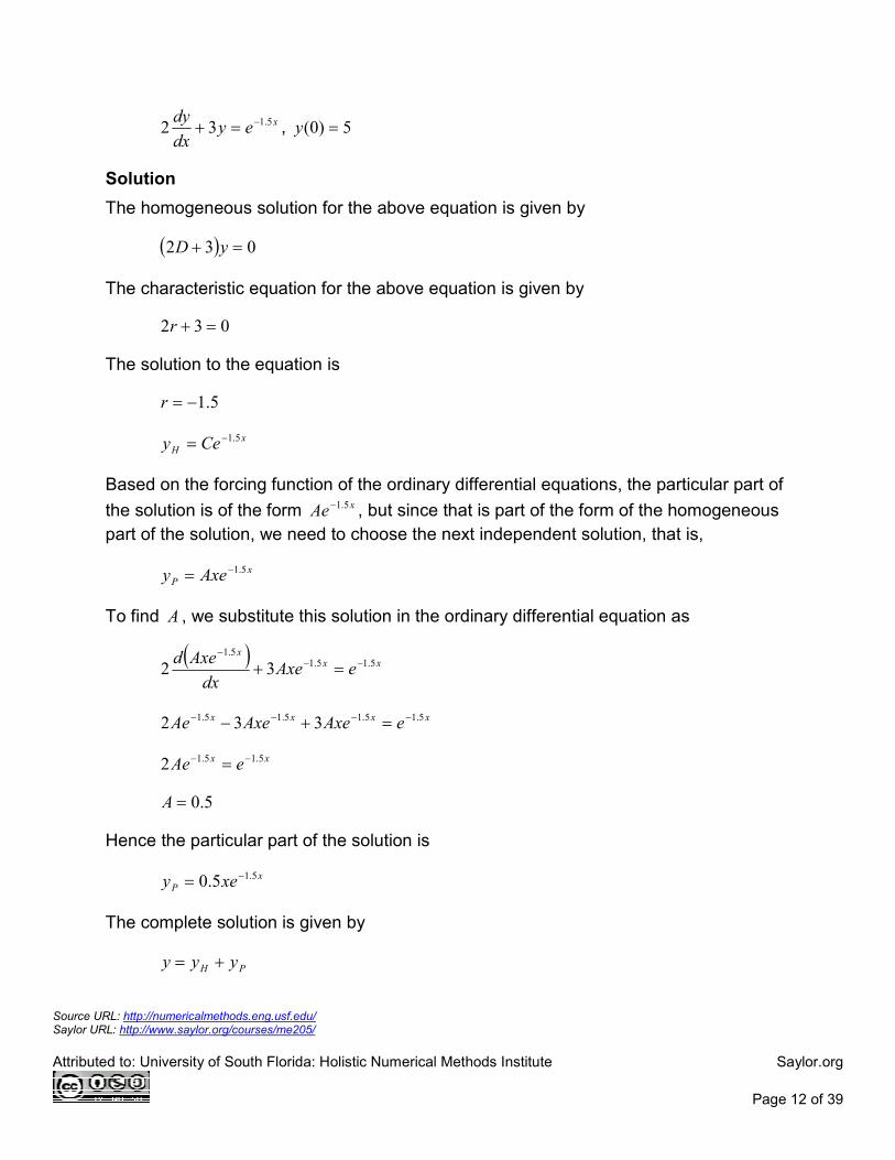
Example 1
Solve
xeydx
dy −=+ 23 , 5)0( =y
Solution
The homogeneous solution for the above equation is given by
( ) 023 =+ yD
The characteristic equation for the above equation is given by
023 =+r
The solution to the equation is
Source URL: http://numericalmethods.eng.usf.edu/ Saylor URL: http://www.saylor.org/courses/me205/
Attributed to: University of South Florida: Holistic Numerical Methods Institute Saylor.org
Page 11 of 39
666667.0−=r
x
H Cey 666667.0−=
The particular part of the solution is of the form xAe−
( ) xx
x
eAedx
Aed −−−
=+ 23
xxx eAeAe −−− =+− 23
xx eAe −− =−
1−=A
Hence the particular part of the solution is
x
P ey −−=
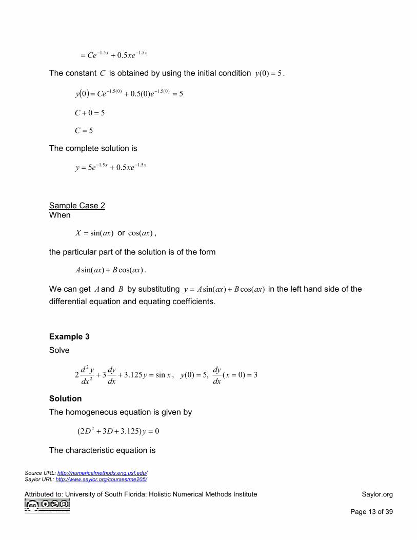
The complete solution is given by
PH yyy +=
xx eCe −− −= 666667.0
The constant C can be obtained by using the initial condition 5)0( =y
( ) 50 00666667.0 =−= −×− eCey
51 =−C
6=C
The complete solution is
xx eey −− −= 666667.06
Example 2
Solve
Source URL: http://numericalmethods.eng.usf.edu/ Saylor URL: http://www.saylor.org/courses/me205/
Attributed to: University of South Florida: Holistic Numerical Methods Institute Saylor.org
Page 12 of 39
xeydx
dy 5.132 −=+ , 5)0( =y
Solution
The homogeneous solution for the above equation is given by
( ) 032 =+ yD
The characteristic equation for the above equation is given by
032 =+r
The solution to the equation is
5.1−=r
x
H Cey 5.1−=
Based on the forcing function of the ordinary differential equations, the particular part of
the solution is of the form xAe 5.1− , but since that is part of the form of the homogeneous
part of the solution, we need to choose the next independent solution, that is,
x
P Axey 5.1−=
To find A , we substitute this solution in the ordinary differential equation as
( ) xx
x
eAxedx
Axed 5.15.15.1
32 −−−
=+
xxxx eAxeAxeAe 5.15.15.15.1 332 −−−− =+−
xx eAe 5.15.12 −− =
5.0=A
Hence the particular part of the solution is
x
P xey 5.15.0 −=
The complete solution is given by
PH yyy +=
Source URL: http://numericalmethods.eng.usf.edu/ Saylor URL: http://www.saylor.org/courses/me205/
Attributed to: University of South Florida: Holistic Numerical Methods Institute Saylor.org
Page 13 of 39
xx xeCe 5.15.1 5.0 −− +=
The constant C is obtained by using the initial condition 5)0( =y .
( ) 5)0(5.00 )0(5.1)0(5.1 =+= −− eCey
50 =+C
5=C
The complete solution is
xx xeey 5.15.1 5.05 −− +=
Sample Case 2 When
)sin(axX = or )cos(ax ,
the particular part of the solution is of the form
)cos()sin( axBaxA + .
We can get Aand B by substituting )cos()sin( axBaxAy += in the left hand side of the
differential equation and equating coefficients.
Example 3
Solve
xydx
dy
dx
ydsin125.332
2
2
=++ , 3)0( ,5)0( === xdx
dyy
Solution
The homogeneous equation is given by
0)125.332( 2 =++ yDD
The characteristic equation is
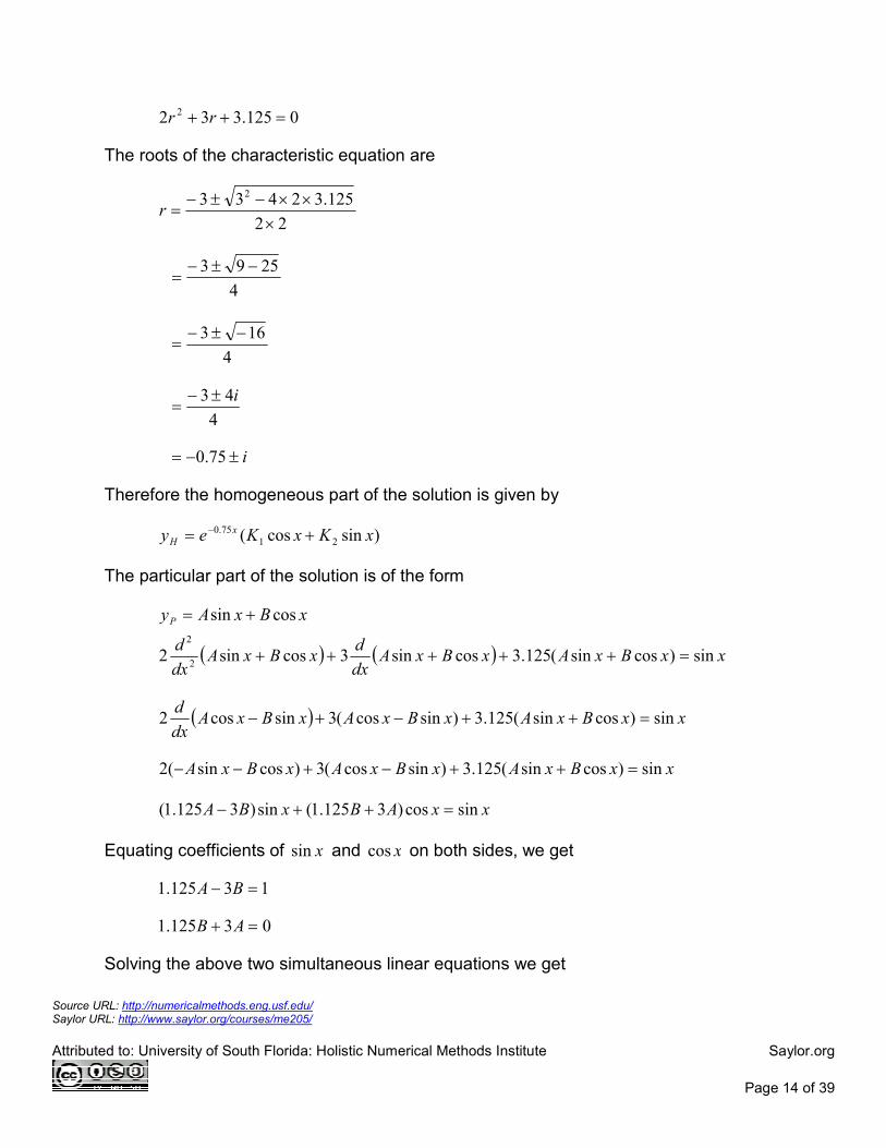
Source URL: http://numericalmethods.eng.usf.edu/ Saylor URL: http://www.saylor.org/courses/me205/
Attributed to: University of South Florida: Holistic Numerical Methods Institute Saylor.org
Page 14 of 39
0125.332 2 =++ rr
The roots of the characteristic equation are
22
125.32433 2
×××−±−
=r
4
2593
−±−=
4
163
−±−=
4
43
i±−=
i±−= 75.0
Therefore the homogeneous part of the solution is given by
)sincos( 21
75.0 xKxKey x
H += −
The particular part of the solution is of the form
xBxAyP cossin +=
( ) ( ) xxBxAxBxAdx
dxBxA
dx
dsin)cossin(125.3cossin3cossin2
2
2
=+++++
( ) xxBxAxBxAxBxAdx
dsin)cossin(125.3)sincos(3sincos2 =++−+−
xxBxAxBxAxBxA sin)cossin(125.3)sincos(3)cossin(2 =++−+−−
xxABxBA sincos)3125.1(sin)3125.1( =++−
Equating coefficients of xsin and xcos on both sides, we get
13125.1 =− BA
03125.1 =+ AB
Solving the above two simultaneous linear equations we get
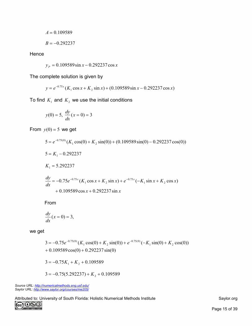
Source URL: http://numericalmethods.eng.usf.edu/ Saylor URL: http://www.saylor.org/courses/me205/
Attributed to: University of South Florida: Holistic Numerical Methods Institute Saylor.org
Page 15 of 39
109589.0=A
292237.0−=B
Hence
xxyP cos292237.0sin109589.0 −=
The complete solution is given by
)cos292237.0sin109589.0()sincos( 21
75.0 xxxKxKey x −++= −
To find 1K and 2K we use the initial conditions
3)0( ,5)0( === xdx
dyy
From 5)0( =y we get
))0cos(292237.0)0sin(109589.0())0sin()0cos((5 21
)0(75.0 −++= − KKe
292237.05 1 −= K
292237.51 =K
xx
xKxKexKxKedx
dy xx
sin292237.0cos109589.0
)cossin()sincos(75.0 21
75.0
21
75.0
++
+−++−= −−
From
,3)0( ==xdx
dy
we get
)0sin(292237.0)0cos(109589.0
))0cos()0sin(( ))0sin()0cos((75.03 21
)0(75.0
21
)0(75.0
++
+−++−= −− KKeKKe
109589.075.03 21 ++−= KK
109589.0)292237.5(75.03 2 ++−= K
Source URL: http://numericalmethods.eng.usf.edu/ Saylor URL: http://www.saylor.org/courses/me205/
Attributed to: University of South Florida: Holistic Numerical Methods Institute Saylor.org
Page 16 of 39
859588.62 =K
The complete solution is
xxxxey x cos292237.0sin109589.0)sin859588.6cos292237.5(75.0 −++= −
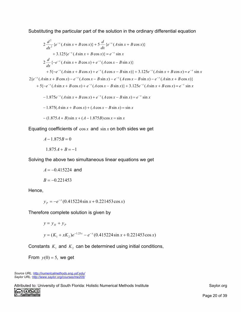
Example 4
Solve
)cos(125.3622
2
xydx
dy
dx
yd=++ , 3)0( ,5)0( === x
dx
dyy
Solution
The homogeneous part of the equations is given by
0)125.362( 2 =++ yDD
The characteristic equation is given by
0125.362 2 =++ rr
)2(2
)125.3)(2(466 2 −±−=r
4
25366 −±−=
4
116 ±−=
829156.05.1 ±−=
329156.2,670844.0 −−=
Therefore, the homogeneous solution Hy is given by
xx
H eKeKy 329156.2
2
670845.0
1
−− +=
The particular part of the solution is of the form
Source URL: http://numericalmethods.eng.usf.edu/ Saylor URL: http://www.saylor.org/courses/me205/
Attributed to: University of South Florida: Holistic Numerical Methods Institute Saylor.org
Page 17 of 39
xBxAyP cossin +=
Substituting the particular part of the solution in the differential equation,
xxBxA
xBxAdx
dxBxA
dx
d
cos)cossin(125.3
)cossin(6)cossin(22
2
=++
+++
xxBxA
xBxAxBxAdx
d
cos)cossin(125.3
)sincos(6)sincos(2
=++
−+−
xxBxA
xBxAxBxA
cos)cossin(125.3
)sincos(6)cossin(2
=++
−+−−
xxABxBA coscos)6125.1(sin)6125.1( =++−
Equating coefficients of xcos and xsin we get
06125.1
16125.1
=−
=+
BA
AB
The solution to the above two simultaneous linear equations are
0301887.0
161006.0
=
=
B
A
Hence the particular part of the solution is
xxyP cos0301887.0sin161006.0 +=
Therefore the complete solution is
PH yyy +=
xxeKeKy xx cos0301887.0sin161006.0)( 329156.2
2
670845.0
1 +++= −−
Constants 1K and 2K can be determined using initial conditions. From 5)0( =y ,
50301887.0)0( 21 =++= KKy
969811.40301887.0521 =−=+ KK
Source URL: http://numericalmethods.eng.usf.edu/ Saylor URL: http://www.saylor.org/courses/me205/
Attributed to: University of South Florida: Holistic Numerical Methods Institute Saylor.org
Page 18 of 39
Now
xx
eKeKdx
dy xx
sin0301887.0cos161006.0
329156.2670845.0 )329156.2(
2
)670845.0(
1
−+
−−= −−
From 3)0( ==xdx
dy
3161006.0329156.2670845.0 21 =+−− KK
161006.03329156.2670845.0 21 +−=+ KK
838994.2329156.2670845.0 21 −=+ KK
We have two linear equations with two unknowns
969811.421 =+ KK
838994.2329156.2670845.0 21 −=+ KK
Solving the above two simultaneous linear equations, we get
692253.81 =K
722442.32 −=K
The complete solution is
.cos0301887.0sin161006.0
)722442.3692253.8( 329156.2670845.0
xx
eey xx
++
−= −−
Sample Case 3 When
bxeX ax sin= or bxeax cos ,
the particular part of the solution is of the form
)cossin( bxBbxAeax + ,
Source URL: http://numericalmethods.eng.usf.edu/ Saylor URL: http://www.saylor.org/courses/me205/
Attributed to: University of South Florida: Holistic Numerical Methods Institute Saylor.org
Page 19 of 39
we can get Aand B by substituting
)cossin( bxBbxAey ax +=
in the left hand side of differential equation and equating coefficients.
Example 5
Solve
xeydx
dy
dx
yd x sin125.3522
2−=++ , 3)0( ,5)0( === x
dx
dyy
Solution
The homogeneous equation is given by
0)125.352( 2 =++ yDD
The characteristic equation is given by
0125.352 2 =++ rr
)2(2
)125.3)(2(455 2 −±−=r
4
25255
−±−=
4
05 ±−=
25.1,25.1 −−=
Since roots are repeated, the homogeneous solution Hy is given by
x
H exKKy )25.1(
21 )( −+=
The particular part of the solution is of the form
)cossin( xBxAey x
P += −
Source URL: http://numericalmethods.eng.usf.edu/ Saylor URL: http://www.saylor.org/courses/me205/
Attributed to: University of South Florida: Holistic Numerical Methods Institute Saylor.org
Page 20 of 39
Substituting the particular part of the solution in the ordinary differential equation
xexBxAe
xBxAedx
dxBxAe
dx
d
xx
xx
sin)}cossin({125.3
)}cossin({5)}cossin({22
2
−−
−−
=++
+++
xexBxAexBxAexBxAe
xBxAexBxAedx
d
xxxx
xx
sin)cossin(125.3)}sincos()cossin({5
)}sincos()cossin({2
−−−−
−−
=++−++−+
−++−
xexBxAexBxAexBxAe
xBxAexBxAexBxAexBxAe
xxxx
xxxx
sin)cossin(125.3)}sincos()cossin({5
)}cossin()sincos()sincos()cossin({2
−−−−
−−−−
=++−++−+
+−−−−−+
xexBxAexBxAexxxsin)sincos()cossin(875.1
−−− =−++−
xxBxAxBxA sin)sincos()cossin(875.1 =−++−
xxBAxBA sincos)875.1(sin)875.1( =−++−
Equating coefficients of xcos and xsin on both sides we get
0875.1 =− BA
1875.1 −=+ BA
Solving the above two simultaneous linear equations we get
415224.0−=A and
221453.0−=B
Hence,
)cos221453.0sin415224.0( xxey x
P +−= −
Therefore complete solution is given by
PH yyy +=
)cos221453.0sin415224.0()( 25.1
21 xxeexKKy xx +−+= −−
Constants 1K and 2K can be determined using initial conditions,
From ,5)0( =y we get
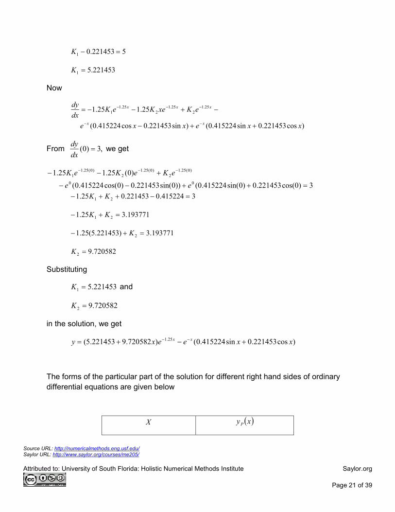
Source URL: http://numericalmethods.eng.usf.edu/ Saylor URL: http://www.saylor.org/courses/me205/
Attributed to: University of South Florida: Holistic Numerical Methods Institute Saylor.org
Page 21 of 39
5221453.01 =−K
221453.51 =K
Now
)cos221453.0sin415224.0()sin221453.0cos415224.0(
25.125.1 25.1
2
25.1
2
25.1
1
xxexxe
eKxeKeKdx
dy
xx
xxx
++−
−+−−=
−−
−−−
From ,3)0( =dx
dy we get
3)0cos(221453.0)0sin(415224.0())0sin(221453.0)0cos(415224.0(
)0(25.125.1
00
)0(25.1
2
)0(25.1
2
)0(25.1
1
=++−−
+−− −−−
ee
eKeKeK
3415224.0221453.025.1 21 =−++− KK
193771.325.1 21 =+− KK
193771.3)221453.5(25.1 2 =+− K
720582.92 =K
Substituting
221453.51 =K and
720582.92 =K
in the solution, we get
)cos221453.0sin415224.0()720582.9221453.5( 25.1 xxeexy xx +−+= −−
The forms of the particular part of the solution for different right hand sides of ordinary
differential equations are given below
X ( )xyP
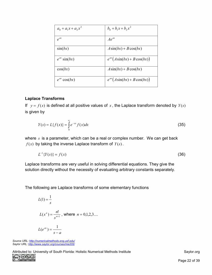
Source URL: http://numericalmethods.eng.usf.edu/ Saylor URL: http://www.saylor.org/courses/me205/
Attributed to: University of South Florida: Holistic Numerical Methods Institute Saylor.org
Page 22 of 39
2
210 xaxaa ++ 2
210 xbxbb ++
axe axAe
)sin(bx )cos()sin( bxBbxA +
)sin(bxeax ( ))cos()sin( bxBbxAeax +
)cos(bx )cos()sin( bxBbxA +
)cos(bxeax ( ))cos()sin( bxBbxAeax +
Laplace Transforms
If )(xfy = is defined at all positive values of x , the Laplace transform denoted by )(sY
is given by
dxxfexfLsY sx )()}({)(0
∫∞
−== (35)
where s is a parameter, which can be a real or complex number. We can get back
)(xf by taking the inverse Laplace transform of )(sY .
)()}({1 xfsYL =− (36)
Laplace transforms are very useful in solving differential equations. They give the
solution directly without the necessity of evaluating arbitrary constants separately.
The following are Laplace transforms of some elementary functions
sL
1)1( =
1
!)(
+=
n
n
s
nxL , where ....3,2,1,0=n
as
eL ax
−=
1)(
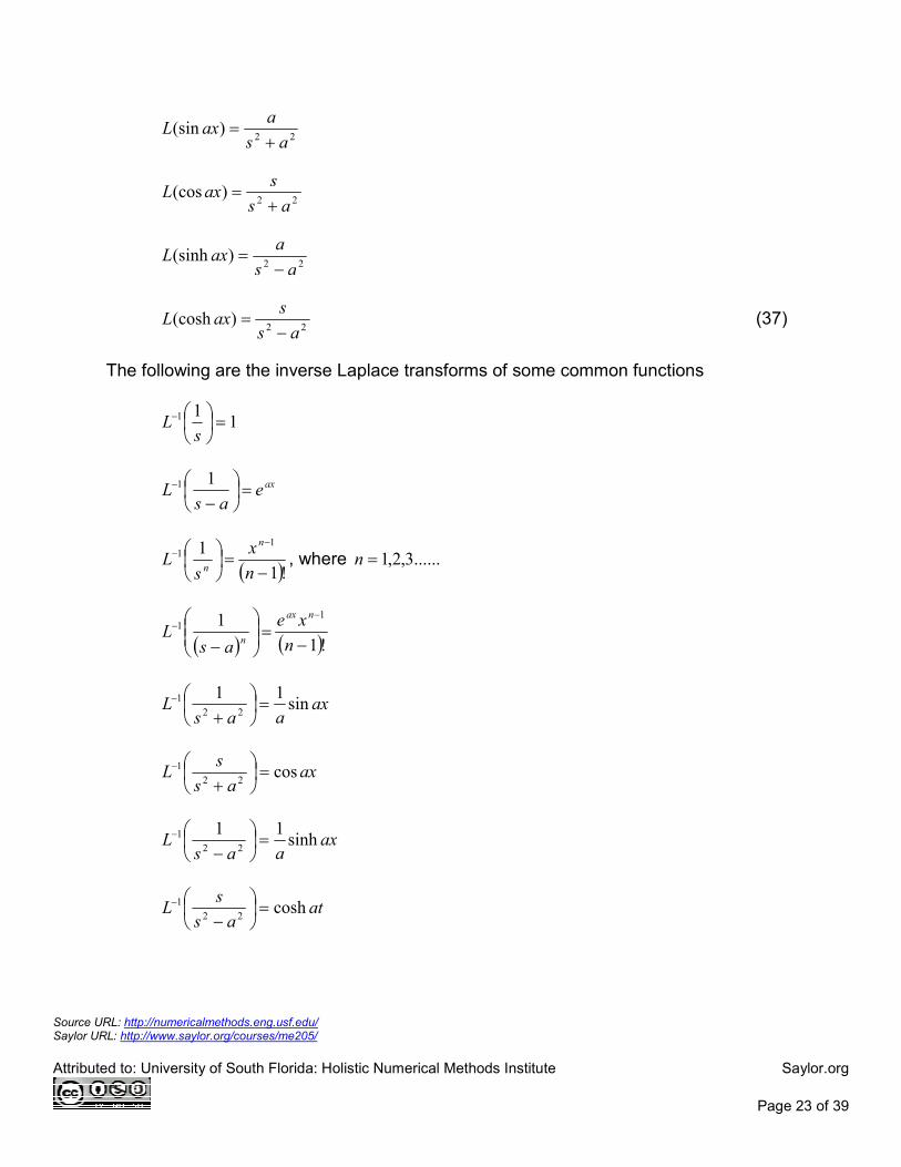
Source URL: http://numericalmethods.eng.usf.edu/ Saylor URL: http://www.saylor.org/courses/me205/
Attributed to: University of South Florida: Holistic Numerical Methods Institute Saylor.org
Page 23 of 39
22
)(sinas
aaxL
+=
22
)(cosas
saxL
+=
22
)(sinhas
aaxL
−=
22
)(coshas
saxL
−= (37)
The following are the inverse Laplace transforms of some common functions
111 =
−
sL
axeas
L =
−
− 11
( )!1
1 11
−=
−−
n
x
sL
n
n, where ......3,2,1=n
( ) ( )!11 1
1
−=
−
−−
n
xe
asL
nax
n
axaas
L sin11
22
1 =
+
−
axas
sL cos
22
1 =
+
−
axaas
L sinh11
22
1 =
−
−
atas
sL cosh
22
1 =
−
−
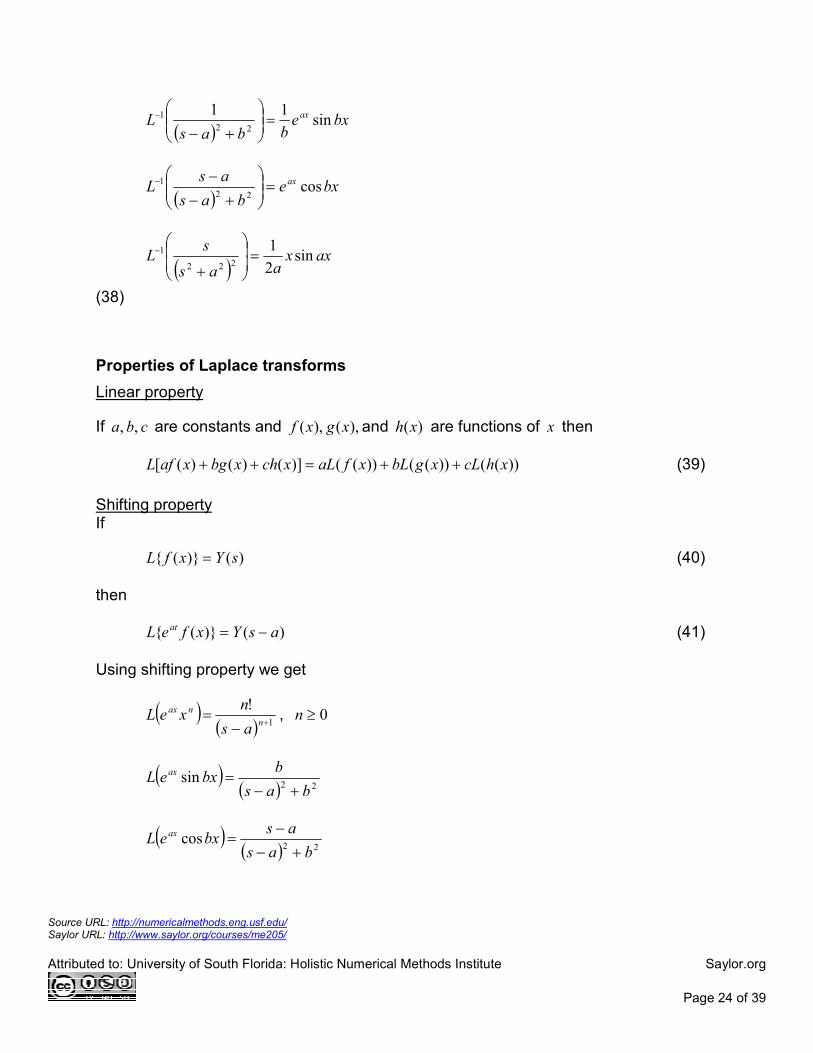
Source URL: http://numericalmethods.eng.usf.edu/ Saylor URL: http://www.saylor.org/courses/me205/
Attributed to: University of South Florida: Holistic Numerical Methods Institute Saylor.org
Page 24 of 39
( )
bxebbas
L ax sin11
22
1 =
+−−
( )
bxebas
asL ax cos
22
1 =
+−
−−
( )
axxaas
sL sin
2
1222
1 =
+
−
(38)
Properties of Laplace transforms
Linear property
If cba , , are constants and ),( ),( xgxf and )(xh are functions of x then
))(())(())(()]()()([ xhcLxgbLxfaLxchxbgxafL ++=++ (39)
Shifting property If
)()}({ sYxfL = (40)
then
)()}({ asYxfeL at −= (41)
Using shifting property we get
( )( ) 1
!+−
=n
nax
as
nxeL , 0≥n
( )( ) 22
sinbas
bbxeL ax
+−=
( )( ) 22
cosbas
asbxeL ax
+−
−=
Source URL: http://numericalmethods.eng.usf.edu/ Saylor URL: http://www.saylor.org/courses/me205/
Attributed to: University of South Florida: Holistic Numerical Methods Institute Saylor.org
Page 25 of 39
( )( ) 22
sinhbas
bbxeL ax
−−=
( )( ) 22
coshbas
asbxeL ax
−−
−= (42)
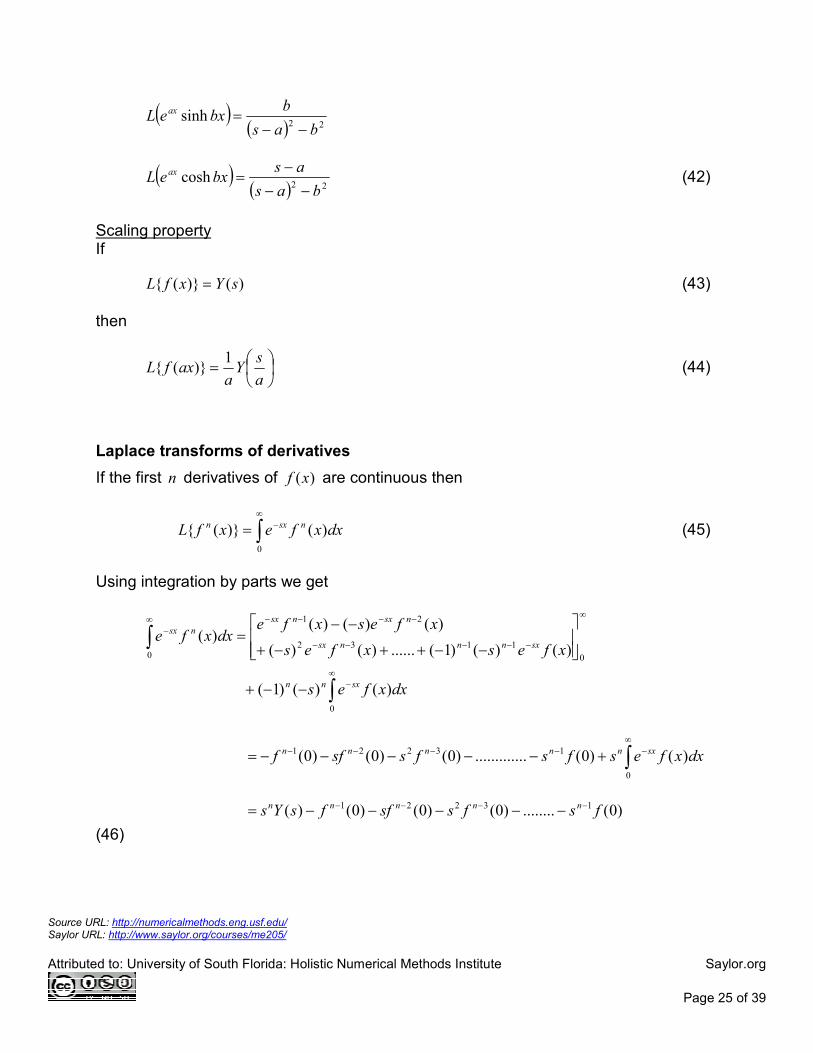
Scaling property If
)()}({ sYxfL = (43)
then
=a
sY
aaxfL
1)}({ (44)
Laplace transforms of derivatives
If the first n derivatives of )(xf are continuous then
∫∞
−=0
)()}({ dxxfexfL nsxn (45)
Using integration by parts we get
∫
∫∞
−
∞∞
−−−−−
−−−−−
−−+
−−++−+
−−=
0
001132
21
)()()1(
)()()1(......)()(
)()()()(
dxxfes
xfesxfes
xfesxfedxxfe
sxnn
sxnnnsx
nsxnsx
nsx
∫∞
−−−−− +−−−−−=0
13221 )()0(.............)0()0()0( dxxfesfsfssff sxnnnnn
)0(........)0()0()0()( 13221 fsfssffsYs nnnnn −−−− −−−−−=
(46)
Source URL: http://numericalmethods.eng.usf.edu/ Saylor URL: http://www.saylor.org/courses/me205/
Attributed to: University of South Florida: Holistic Numerical Methods Institute Saylor.org
Page 26 of 39
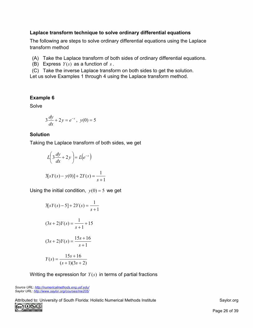
Laplace transform technique to solve ordinary differential equations
The following are steps to solve ordinary differential equations using the Laplace
transform method
(A) Take the Laplace transform of both sides of ordinary differential equations. (B) Express )(sY as a function of s .
(C) Take the inverse Laplace transform on both sides to get the solution. Let us solve Examples 1 through 4 using the Laplace transform method.
Example 6
Solve
xeydx
dy −=+ 23 , 5)0( =y
Solution
Taking the Laplace transform of both sides, we get
( )xeLydx
dyL −=
+ 23
1
1)(2)]0()([3
+=+−s
sYyssY
Using the initial condition, 5)0( =y we get
1
1)(2]5)([3
+=+−s
sYssY
151
1)()23( +
+=+s
sYs
1
1615)()23(
++
=+s
ssYs
)23)(1(
1615)(
+++
=ss
ssY
Writing the expression for )(sY in terms of partial fractions
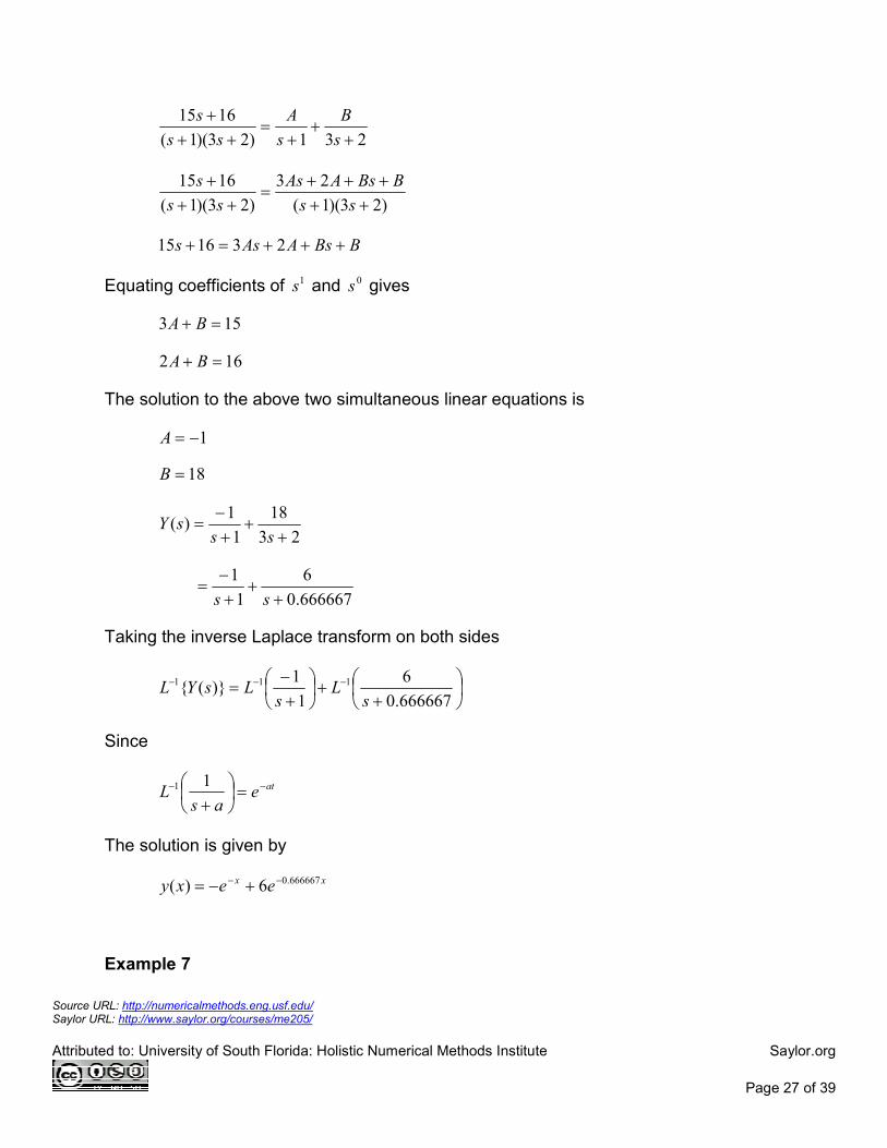
Source URL: http://numericalmethods.eng.usf.edu/ Saylor URL: http://www.saylor.org/courses/me205/
Attributed to: University of South Florida: Holistic Numerical Methods Institute Saylor.org
Page 27 of 39
231)23)(1(
1615
++
+=
+++
s
B
s
A
ss
s
)23)(1(
23
)23)(1(
1615
+++++
=++
+ss
BBsAAs
ss
s
BBsAAss +++=+ 231615
Equating coefficients of 1s and 0s gives
153 =+ BA
162 =+ BA
The solution to the above two simultaneous linear equations is
1−=A
18=B
23
18
1
1)(
++
+−
=ss
sY
666667.0
6
1
1
++
+−
=ss
Taking the inverse Laplace transform on both sides
+
+
+−
= −−−
666667.0
6
1
1)}({ 111
sL
sLsYL
Since
ateas
L −− =
+11
The solution is given by
xx eexy 666667.06)( −− +−=
Example 7
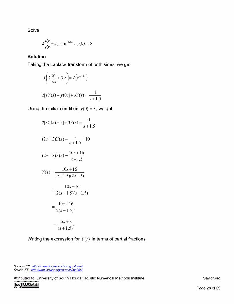
Source URL: http://numericalmethods.eng.usf.edu/ Saylor URL: http://www.saylor.org/courses/me205/
Attributed to: University of South Florida: Holistic Numerical Methods Institute Saylor.org
Page 28 of 39
Solve
xeydx
dy 5.132 −=+ , 5)0( =y
Solution
Taking the Laplace transform of both sides, we get
( )xeLydx
dyL 5.132 −=
+
5.1
1)(3)]0()([2
+=+−s
sYyssY
Using the initial condition 5)0( =y , we get
5.1
1)(3]5)([2
+=+−s
sYssY
105.1
1)()32( +
+=+s
sYs
5.1
1610)()32(
++
=+s
ssYs
)32)(5.1(
1610)(
+++
=ss
ssY
)5.1)(5.1(2
1610
+++
=ss
s
2)5.1(2
1610
+
+=
s
s
2)5.1(
85
+
+=
s
s
Writing the expression for )(sY in terms of partial fractions
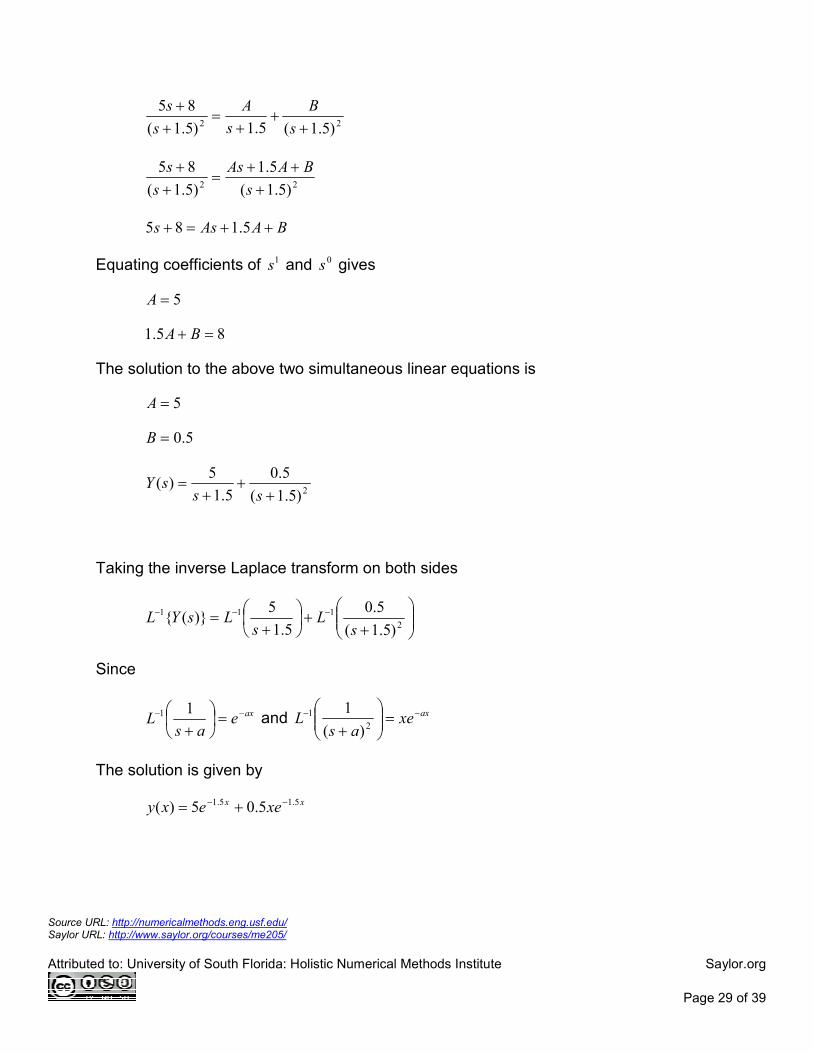
Source URL: http://numericalmethods.eng.usf.edu/ Saylor URL: http://www.saylor.org/courses/me205/
Attributed to: University of South Florida: Holistic Numerical Methods Institute Saylor.org
Page 29 of 39
22 )5.1(5.1)5.1(
85
++
+=
+
+
s
B
s
A
s
s
22 )5.1(
5.1
)5.1(
85
+
++=
+
+
s
BAAs
s
s
BAAss ++=+ 5.185
Equating coefficients of 1s and 0s gives
5=A
85.1 =+ BA
The solution to the above two simultaneous linear equations is
5=A
5.0=B
2)5.1(
5.0
5.1
5)(
++
+=
sssY
Taking the inverse Laplace transform on both sides
++
+
= −−−2
111
)5.1(
5.0
5.1
5)}({
sL
sLsYL
Since
axeas
L −− =
+11 and axxe
asL −− =
+ 2
1
)(
1
The solution is given by
xx xeexy 5.15.1 5.05)( −− +=
Source URL: http://numericalmethods.eng.usf.edu/ Saylor URL: http://www.saylor.org/courses/me205/
Attributed to: University of South Florida: Holistic Numerical Methods Institute Saylor.org
Page 30 of 39
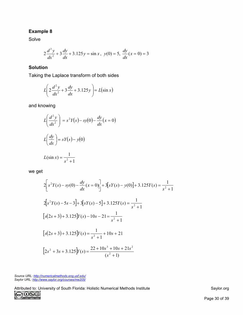
Example 8
Solve
xydx
dy
dx
ydsin125.332
2
2
=++ , 3)0( ,5)0( === xdx
dyy
Solution
Taking the Laplace transform of both sides
( )xLydx
dy
dx
ydL sin125.332
2
2
=
++
and knowing
2
2
dx
ydL ( ) ( ) ( )002 =−−= x
dx
dysysYs
dx
dyL ( ) ( )0yssY −=
1
1)(sin
2 +=s
xL
we get
[ ]1
1)(125.3)0()(3)0()0()(2
2
2
+=+−+
=−−s
sYyssYxdx
dysysYs
[ ] [ ]1
1)(125.35)(335)(2
2
2
+=+−+−−s
sYssYssYs
( )[ ]1
12110)(125.332
2 +=−−++s
ssYss
( )[ ] 21101
1)(125.332
2++
+=++ ss
sYss
[ ])1(
21101022)(125.332
2
232
+
+++=++
s
ssssYss
Source URL: http://numericalmethods.eng.usf.edu/ Saylor URL: http://www.saylor.org/courses/me205/
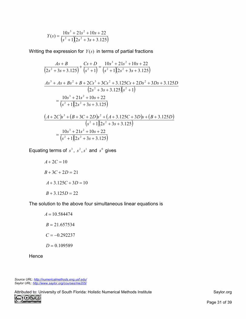
Attributed to: University of South Florida: Holistic Numerical Methods Institute Saylor.org
Page 31 of 39
( )( )125.3321
22102110)(
22
23
+++
+++=
sss
ssssY
Writing the expression for )(sY in terms of partial fractions
( ) ( ) ( )( )125.3321
22102110
1125.332 22
23
22 +++
+++=
+
++
++
+
sss
sss
s
DCs
ss
BAs
( )( )
( )( )125.3321
22102110
1125.332
125.332125.332
22
23
22
22323
+++
+++=
+++
+++++++++
sss
sss
sss
DDsDsCsCsCsBBsAsAs
( ) ( ) ( ) ( )( )( )
( )( )125.3321
22102110
125.3321
125.33125.3232
22
23
22
23
+++
+++=
+++
+++++++++
sss
sss
sss
DBsDCAsDCBsCA
Equating terms of 3s , 12 , ss and 0s gives
102 =+ CA
2123 =++ DCB
103125.3 =++ DCA
22125.3 =+ DB
The solution to the above four simultaneous linear equations is
584474.10=A
657534.21=B
292237.0−=C
109589.0=D
Hence
Source URL: http://numericalmethods.eng.usf.edu/ Saylor URL: http://www.saylor.org/courses/me205/
Attributed to: University of South Florida: Holistic Numerical Methods Institute Saylor.org
Page 32 of 39
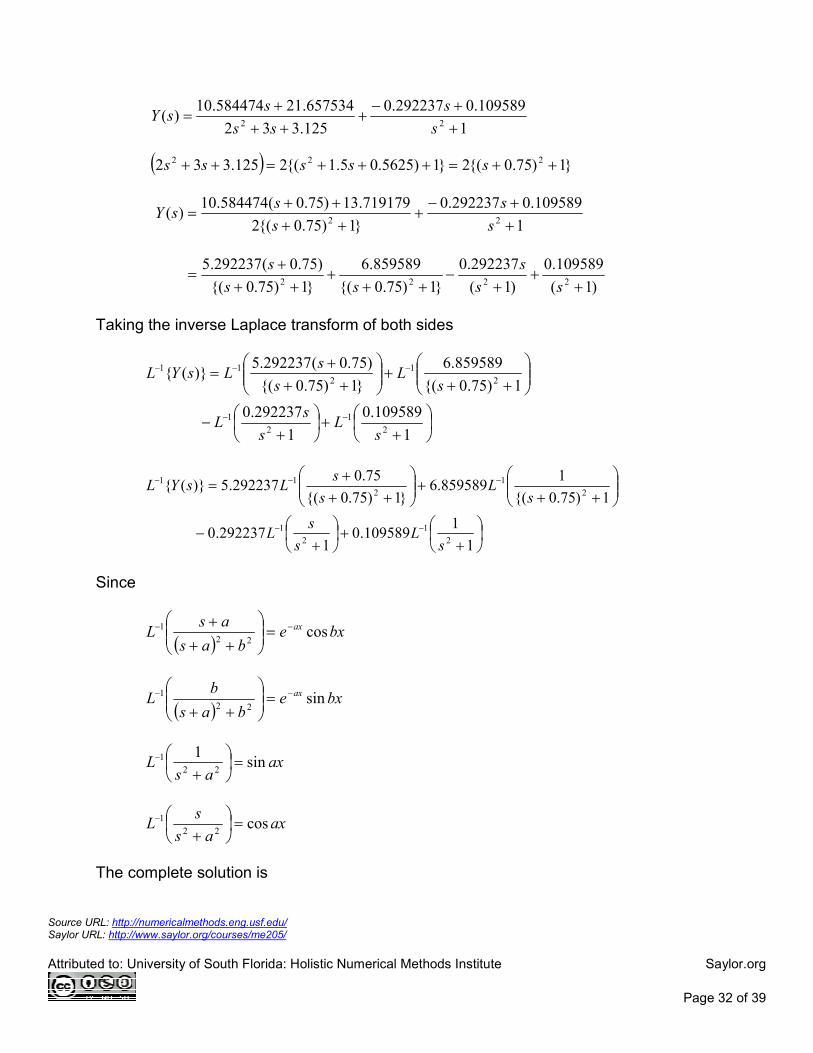
1
109589.0292237.0
125.332
657534.21584474.10)(
22 +
+−+
++
+=
s
s
ss
ssY
( ) }1)75.0{(2}1)5625.05.1{(2125.332 222 ++=+++=++ sssss
1
109589.0292237.0
}1)75.0{(2
719179.13)75.0(584474.10)(
22 +
+−+
++
++=
s
s
s
ssY
)1(
109589.0
)1(
292237.0
}1)75.0{(
859589.6
}1)75.0{(
)75.0(292237.5
2222 ++
+−
+++
++
+=
ss
s
ss
s
Taking the inverse Laplace transform of both sides
+
+
+
−
+++
++
+=
−−
−−−
1
109589.0
1
292237.0
1)75.0{(
859589.6
}1)75.0{(
)75.0(292237.5)}({
2
1
2
1
2
1
2
11
sL
s
sL
sL
s
sLsYL
+
+
+
−
+++
++
+=
−−
−−−
1
1109589.0
1292237.0
1)75.0{(
1859589.6
}1)75.0{(
75.0292237.5)}({
2
1
2
1
2
1
2
11
sL
s
sL
sL
s
sLsYL
Since
( )
bxebas
asL ax cos
22
1 −− =
++
+
( )
bxebas
bL ax sin
22
1 −− =
++
axas
L sin1
22
1 =
+
−
axas
sL cos
22
1 =
+
−
The complete solution is
Source URL: http://numericalmethods.eng.usf.edu/ Saylor URL: http://www.saylor.org/courses/me205/
Attributed to: University of South Florida: Holistic Numerical Methods Institute Saylor.org
Page 33 of 39
xx
xexexy xx
sin109589.0cos292237.0
sin8595859.6cos292237.5)( 75.075.0
+−
+= −−
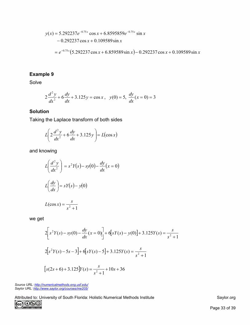
( ) xxxxe x sin109589.0cos292237.0sin859589.6cos292237.5 75.0 +−+= −
Example 9
Solve
xydx
dy
dx
ydcos125.362
2
2
=++ , 3)0( ,5)0( === xdx
dyy
Solution
Taking the Laplace transform of both sides
( )xLydx
dy
dx
ydL cos125.362
2
2
=
++
and knowing
2
2
dx
ydL ( ) ( ) ( )002 =−−= x
dx
dysysYs
dx
dyL ( ) ( )0yssY −=
1
)(cos2 +
=s
sxL
we get
[ ]1
)(125.3)0()(6)0()0()(22
2
+=+−+
=−−s
ssYyssYx
dx
dysysYs
[ ] [ ]1
)(125.35)(635)(22
2
+=+−+−−s
ssYssYssYs
[ ] 3610
1)(125.3)62(
2++
+=++ ss
ssYss
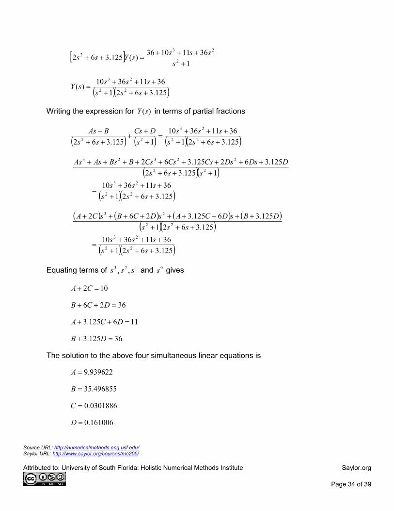
Source URL: http://numericalmethods.eng.usf.edu/ Saylor URL: http://www.saylor.org/courses/me205/
Attributed to: University of South Florida: Holistic Numerical Methods Institute Saylor.org
Page 34 of 39
[ ]1
36111036)(125.362
2
232
+
+++=++
s
ssssYss
( )( )125.3621
36113610)(
22
23
+++
+++=
sss
ssssY
Writing the expression for )(sY in terms of partial fractions
( ) ( ) ( )( )125.3621
36113610
1125.362 22
23
22 +++
+++=
+
++
++
+
sss
sss
s
DCs
ss
BAs
( )( )
( )( )125.3621
36113610
1125.362
125.362125.362
22
23
22
22323
+++
+++=
+++
+++++++++
sss
sss
sss
DDsDsCsCsCsBBsAsAs
( ) ( ) ( ) ( )( )( )
( )( )125.3621
36113610
125.3621
125.36125.3262
22
23
22
23
+++
+++=
+++
+++++++++
sss
sss
sss
DBsDCAsDCBsCA
Equating terms of 3s , 12 , ss and 0s gives
102 =+ CA
3626 =++ DCB
116125.3 =++ DCA
36125.3 =+ DB
The solution to the above four simultaneous linear equations is
939622.9=A
496855.35=B
0301886.0=C
161006.0=D
Source URL: http://numericalmethods.eng.usf.edu/ Saylor URL: http://www.saylor.org/courses/me205/
Attributed to: University of South Florida: Holistic Numerical Methods Institute Saylor.org
Page 35 of 39
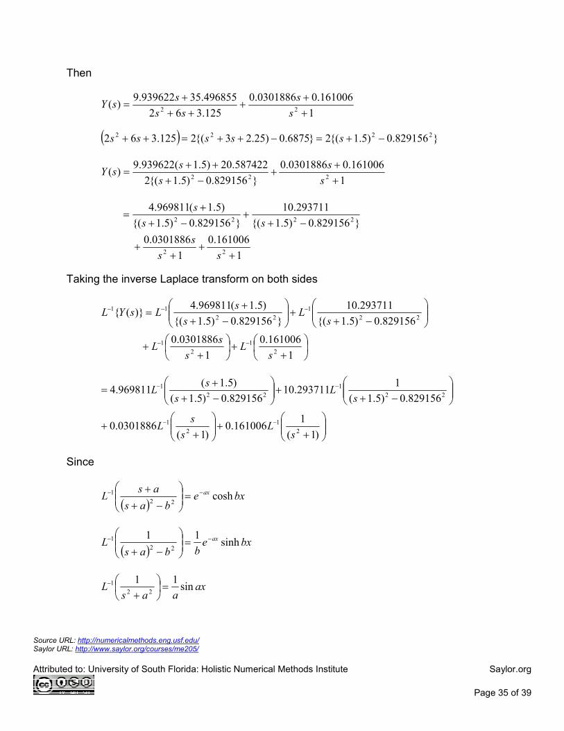
Then
1
161006.00301886.0
125.362
496855.35939622.9)(
22 +
++
++
+=
s
s
ss
ssY
( ) }829156.0)5.1{(2}6875.0)25.23{(2125.362 2222 −+=−++=++ sssss
1
161006.00301886.0
}829156.0)5.1{(2
587422.20)5.1(939622.9)(
222 +
++
−+
++=
s
s
s
ssY
1
161006.0
1
0301886.0
}829156.0)5.1{(
293711.10
}829156.0)5.1{(
)5.1(969811.4
22
2222
++
++
−++
−+
+=
ss
s
ss
s
Taking the inverse Laplace transform on both sides
+
+
+
+
−++
−+
+=
−−
−−−
1
161006.0
1
0301886.0
829156.0)5.1{(
293711.10
}829156.0)5.1{(
)5.1(969811.4)}({
2
1
2
1
22
1
22
11
sL
s
sL
sL
s
sLsYL
−+
+
−++
= −−22
1
22
1
829156.0)5.1(
1293711.10
829156.0)5.1(
)5.1(969811.4
sL
s
sL
++
++ −−
)1(
1161006.0
)1(0301886.0
2
1
2
1
sL
s
sL
Since
( )
bxebas
asL ax cosh
22
1 −− =
−+
+
( )
bxebbas
L ax sinh11
22
1 −− =
−+
axaas
L sin11
22
1 =
+
−
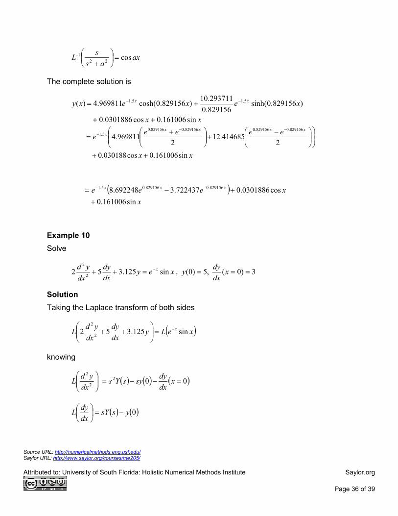
Source URL: http://numericalmethods.eng.usf.edu/ Saylor URL: http://www.saylor.org/courses/me205/
Attributed to: University of South Florida: Holistic Numerical Methods Institute Saylor.org
Page 36 of 39
axas
sL cos
22
1 =
+
−
The complete solution is
xx
xexexy xx
sin161006.0cos0301886.0
)829156.0sinh(829156.0
293711.10)829156.0cosh(969811.4)( 5.15.1
++
+= −−
xx
eeeee
xxxxx
sin161006.0cos030188.0
2414685.12
2969811.4
829156.0829156.0829156.0829156.05.1
++
−+
+=
−−−
( )
x
xeee xxx
sin161006.0
cos0301886.0722437.3692248.8 829156.0829156.05.1
+
+−= −−
Example 10
Solve
xeydx
dy
dx
yd x sin125.3522
2−=++ , 3)0( ,5)0( === x
dx
dyy
Solution
Taking the Laplace transform of both sides
( )xeLydx
dy
dx
ydL x sin125.352
2
2−=
++
knowing
2
2
dx
ydL ( ) ( ) ( )002 =−−= x
dx
dysysYs
dx
dyL ( ) ( )0yssY −=
Source URL: http://numericalmethods.eng.usf.edu/ Saylor URL: http://www.saylor.org/courses/me205/
Attributed to: University of South Florida: Holistic Numerical Methods Institute Saylor.org
Page 37 of 39
1)1(
1)sin(
2 ++=−
sxeL x
we get
[ ]
[ ] [ ]1)1(
1)(125.35)(535)(2
1)1(
1)(125.3)0()(5)0()0()(2
2
2
2
2
++=+−+−−
++=+−+
=−−
ssYssYssYs
ssYyssYx
dx
dysysYs
( )[ ]1)1(
13110)(125.352
2 ++=−−++
sssYss
[ ] 31101)1(
1)(125.3)52(
2++
++=++ s
ssYss
[ ]22
51821063)(125.352
2
232
++
+++=++
ss
ssssYss
( )( )125.35222
63825110)(
22
23
++++
+++=
ssss
ssssY
Writing the expression for )(sY in terms of partial fractions
( )( )125.35222
63825110
22125.352 22
23
22 ++++
+++=
++
++
++
+
ssss
sss
ss
DCs
ss
BAs
( )( )
( )( )125.35222
63825110
22125.352
2222125.352125.352
22
23
22
223223
++++
+++=
++++
+++++++++++
ssss
sss
ssss
BBsBsAsAsAsDDsDsCsCsCs
( ) ( ) ( ) ( )( )( )
( )( )125.35222
63825110
125.35222
2125.3225125.32252
22
23
22
23
++++
+++=
++++
+++++++++++
ssss
sss
ssss
BDsBADCsBADCsAC
Source URL: http://numericalmethods.eng.usf.edu/ Saylor URL: http://www.saylor.org/courses/me205/
Attributed to: University of South Florida: Holistic Numerical Methods Institute Saylor.org
Page 38 of 39
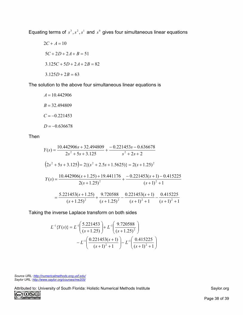
Equating terms of 3s , 12 , ss and 0s gives four simultaneous linear equations
102 =+ AC
51225 =+++ BADC
82225125.3 =+++ BADC
632125.3 =+ BD
The solution to the above four simultaneous linear equations is
442906.10=A
494809.32=B
221453.0−=C
636678.0−=D
Then
22
636678.0221453.0
125.352
494809.32442906.10)(
22 ++
−−+
++
+=
ss
s
ss
ssY
( ) 222 )25.1(2)}5625.15.2{(2125.352 +=++=++ sssss
1)1(
415225.0)1(221453.0
)25.1(2
441176.19)25.1(442906.10)(
22 ++
−+−+
+
++=
s
s
s
ssY
1)1(
415225.0
1)1(
)1(221453.0
)25.1(
720588.9
)25.1(
)25.1(221453.5
2222 ++−
++
+−
++
+
+=
ss
s
ss
s
Taking the inverse Laplace transform on both sides
++−
+++
−
++
+=
−−
−−−
1)1(
415225.0
1)1(
)1(221453.0
)25.1(
720588.9
)25.1(
221453.5)}({
2
1
2
1
2
111
sL
s
sL
sL
sLsYL
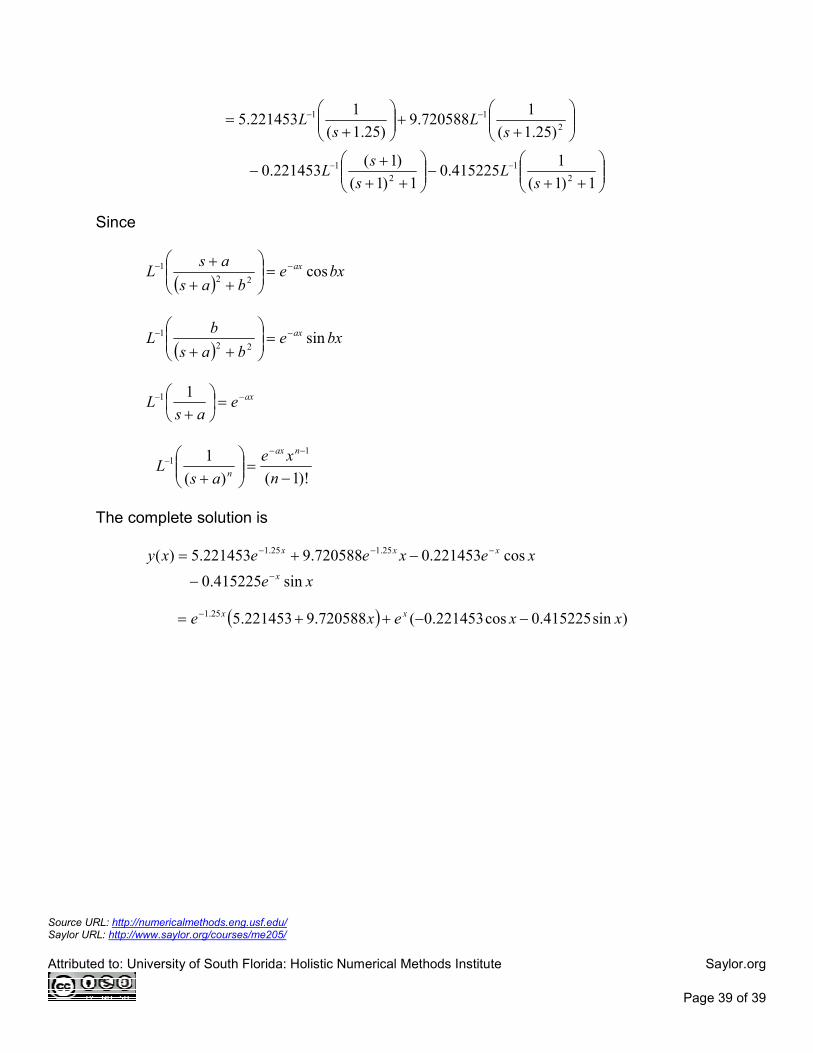
Source URL: http://numericalmethods.eng.usf.edu/ Saylor URL: http://www.saylor.org/courses/me205/
Attributed to: University of South Florida: Holistic Numerical Methods Institute Saylor.org
Page 39 of 39
++−
+++
−
++
+=
−−
−−
1)1(
1415225.0
1)1(
)1(221453.0
)25.1(
1720588.9
)25.1(
1221453.5
2
1
2
1
2
11
sL
s
sL
sL
sL
Since
( )
bxebas
asL ax cos
22
1 −− =
++
+
( )
bxebas
bL ax sin
22
1 −− =
++
axeas
L −− =
+11
)!1()(
1 11
−=
+
−−−
n
xe
asL
nax
n
The complete solution is
xe
xexeexy
x
xxx
sin415225.0
cos221453.0720588.9221453.5)( 25.125.1
−
−−−
−
−+=
( ) )sin415225.0cos221453.0(720588.9221453.5 25.1 xxexe xx −−++= −