A Primer on Profit Maximization - ScholarWorks

Central Washington UniversityScholarWorks@CWU

All Faculty Scholarship for the College of Business College of Business

Fall 2011

A Primer on Profit MaximizationRobert CarbaughCentral Washington University, [email protected]

Tyler PranteLos Angeles Valley College

Follow this and additional works at: http://digitalcommons.cwu.edu/cobfac

Part of the Economic Theory Commons, and the Higher Education Commons

This Article is brought to you for free and open access by the College of Business at ScholarWorks@CWU. It has been accepted for inclusion in AllFaculty Scholarship for the College of Business by an authorized administrator of ScholarWorks@CWU.

Recommended CitationCarbaugh, Robert and Tyler Prante. (2011). A primer on profit maximization. Journal for Economic Educators, 11(2), 34-45.

http://digitalcommons.cwu.edu?utm_source=digitalcommons.cwu.edu%2Fcobfac%2F123&utm_medium=PDF&utm_campaign=PDFCoverPages

http://digitalcommons.cwu.edu/cobfac?utm_source=digitalcommons.cwu.edu%2Fcobfac%2F123&utm_medium=PDF&utm_campaign=PDFCoverPages

http://digitalcommons.cwu.edu/cob?utm_source=digitalcommons.cwu.edu%2Fcobfac%2F123&utm_medium=PDF&utm_campaign=PDFCoverPages

http://digitalcommons.cwu.edu/cobfac?utm_source=digitalcommons.cwu.edu%2Fcobfac%2F123&utm_medium=PDF&utm_campaign=PDFCoverPages

http://network.bepress.com/hgg/discipline/344?utm_source=digitalcommons.cwu.edu%2Fcobfac%2F123&utm_medium=PDF&utm_campaign=PDFCoverPages

http://network.bepress.com/hgg/discipline/1245?utm_source=digitalcommons.cwu.edu%2Fcobfac%2F123&utm_medium=PDF&utm_campaign=PDFCoverPages

34 JOURNAL FOR ECONOMIC EDUCATORS, 11(2), FALL 2011

A PRIMER ON PROFIT MAXIMIZATION

Robert Carbaugh1 and Tyler Prante

2

Abstract

Although textbooks in intermediate microeconomics and managerial economics discuss the first-

order condition for profit maximization (marginal revenue equals marginal cost) for pure

competition and monopoly, they tend to ignore the second-order condition (marginal cost cuts

marginal revenue from below). Mathematical economics textbooks also tend to provide only

tangential treatment of the necessary and sufficient conditions for profit maximization. This

paper fills the void in the textbook literature by combining mathematical and graphical analysis

to more fully explain the profit maximizing hypothesis under a variety of market structures and

cost conditions. It is intended to be a useful primer for all students taking intermediate level

courses in microeconomics, managerial economics, and mathematical economics. It also will be

helpful for students in Master’s and Ph.D. programs in economics and in MBA programs.

Moreover, the paper provides instructors with an effective supplement when explaining the

profit-maximization concept to students.3

Key Words: profit maximization, microeconomics

JEL Classification: A2, D2

Introduction

For about a century, the assumption that a firm maximizes profit (total revenue minus

total cost) has been at the forefront of neoclassical economic theory. This assumption is the

guiding principle underlying every firm’s production. An important aspect of this assumption is

that firms maximize profit by setting output where marginal cost (MC) equals marginal revenue

(MR). This equality holds regardless of the market structure under study—that is, perfect

competition, monopoly, monopolistic competition, or oligopoly. While the implications of

profit maximization are different for different market structures, the process of maximizing profit

is essentially the same. The problem for the firm is to determine where to locate output, given

costs and the demand for the product to be sold.

In the simplest version of the theory of the firm, it is assumed that a firm’s owner-

manager attempts to maximize the firm’s short-run profits (current profits and profits in

the near future). More sophisticated models of profit maximization replace the goal of

maximizing short-run profits with the goal of maximizing long-run profits, which reflect the

1 Professor and Co-Chair, Department of Economics, Central Washington University

2 Assistant Professor, Department of Economics, Los Angeles Valley College

3 We wish to thank Professors John Olienyk, Darwin Wassink, Gerald Gunn, Tim Dittmer,

Koushik Ghosh and an anonymous reviewer for comments and suggestions.


present value of the firm’s expected profits. In these models, the MR = MC concept plays an

important role in analyzing the behavior of firms.

Nevertheless, the profit-maximization assumption has been criticized on the grounds that

managers often aim to attain merely “satisfactory” profits for the stockholders of the firm rather

than maximum profits. Moreover, managers may pursue goals other than profit maximization,

including sales maximization, personal welfare, and social welfare, all of which tend to reduce

profit. In spite of these challenges, the MR = MC model of profit maximization is the dominant

model used by the economics profession to explain firm behavior.

Profit maximization is emphasized in all microeconomics courses, from principles classes

to graduate courses. Principles textbooks (e.g., Mankiw, 2009; Krugman and Wells, 2009;

Hubbard and O’Brien, 2007) provide an introduction to the topic by using graphical analysis

showing that a firm’s total profit is maximized at the output where MR is equal to MC. Because

principles texts are intended to fulfill the needs of beginning students (as they should), they

address this topic only by considering the first-order condition for profit maximization, MR =

MC. This leaves the second-order condition for profit maximization to be explained by more

advanced texts; that is, when MR = MC, profit is maximized if MC cuts MR from below. When

surveying intermediate microeconomics texts, however, we found that they generally do not shed

much light on the second-order condition.

Of the eight leading intermediate microeconomics texts that we surveyed, all use

graphical analysis to illustrate the first-order condition for profit maximization for the market

models of perfect competition and monopoly, as seen in Tables 1 and 2. One text (Besanko and

Braeutigam, 2005) uses graphical analysis to portray the second-order condition for perfect

competition, but not for monopoly. Another text (Eaton, Eaton and Allen, 2009) uses graphical

analysis to tangentially discuss the second-order condition for perfect competition and

monopoly; in a footnote, it also uses calculus to identify the second-order condition for

monopoly. Its treatment of this topic is limited to the case where marginal cost is rising at the

profit-maximizing output. But what if MC is decreasing?

A possible example of decreasing MC arises in the current weak economies of the United

States and other countries. Given excess capacity, as firms such as Ford Motor Co. expand

production, the benefits of mass production kick in and MC may decline. As output increases,

MC may fall below MR, but the firm will maximize profit by increasing output until rising MC

eventually meets MR.

We also surveyed leading undergraduate mathematical economics texts to determine the

extent to which they discuss the necessary and sufficient conditions for profit maximization.

Initially we thought that these texts would present these conditions in a comprehensive manner

so as to make the topic obvious to students; therefore, why should we write this paper?

However, we found coverage of this topic to be tangential. All of the texts that we reviewed

(Dadkhah 2007, Sydsaeter and Hammond 2006, Dowling 2001, Silberberg and Suen 2001, and

Simon and Blume 1994) use calculus to illustrate the general nature of first- and second-order

conditions, which can be applied to a variety of topics. But these texts do not apply in a student

friendly manner these conditions to profit maximization for pure competition and monopoly.

Moreover, not all students taking economics courses will take a course in mathematical

economics dealing with first- and second-order conditions. Simply put, there is a void in the

treatment of the necessary and sufficient conditions for profit maximization that exists not only

in intermediate microeconomics textbooks, but also in those for mathematical economics and

managerial economics.


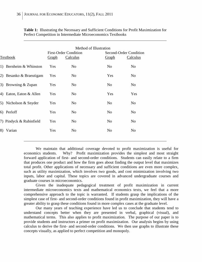
Table 1: Illustrating the Necessary and Sufficient Conditions for Profit Maximization for

Perfect Competition in Intermediate Microeconomics Textbooks

________________________________________________________________________

Method of Illustration

First-Order Condition Second-Order Condition

Textbook Graph Calculus Graph Calculus

1) Bernheim & Whinston Yes No No No

2) Besanko & Braeutigam Yes No Yes No

3) Browning & Zupan Yes No No No

4) Eaton, Eaton & Allen Yes No Yes Yes

5) Nicholson & Snyder Yes No No No

6) Perloff Yes No No No

7) Pindyck & Rubinfield Yes No No No

8) Varian Yes No No No

________________________________________________________________________

We maintain that additional coverage devoted to profit maximization is useful for

economics students. Why? Profit maximization provides the simplest and most straight

forward application of first- and second-order conditions. Students can easily relate to a firm

that produces one product and how the firm goes about finding the output level that maximizes

total profit. Other applications of necessary and sufficient conditions are even more complex,

such as utility maximization, which involves two goods, and cost minimization involving two

inputs, labor and capital. These topics are covered in advanced undergraduate courses and

graduate courses in microeconomics.

Given the inadequate pedagogical treatment of profit maximization in current

intermediate microeconomics texts and mathematical economics texts, we feel that a more

comprehensive approach to the topic is warranted. If students grasp the implications of the

simplest case of first- and second-order conditions found in profit maximization, they will have a

greater ability to grasp these conditions found in more complex cases at the graduate level.

Our many years of teaching experience have led us to conclude that students tend to

understand concepts better when they are presented in verbal, graphical (visual), and

mathematical terms. This also applies to profit maximization. The purpose of our paper is to

provide students and instructors a primer on profit maximization. Our analysis begins by using

calculus to derive the first- and second-order conditions. We then use graphs to illustrate these

concepts visually, as applied to perfect competition and monopoly.


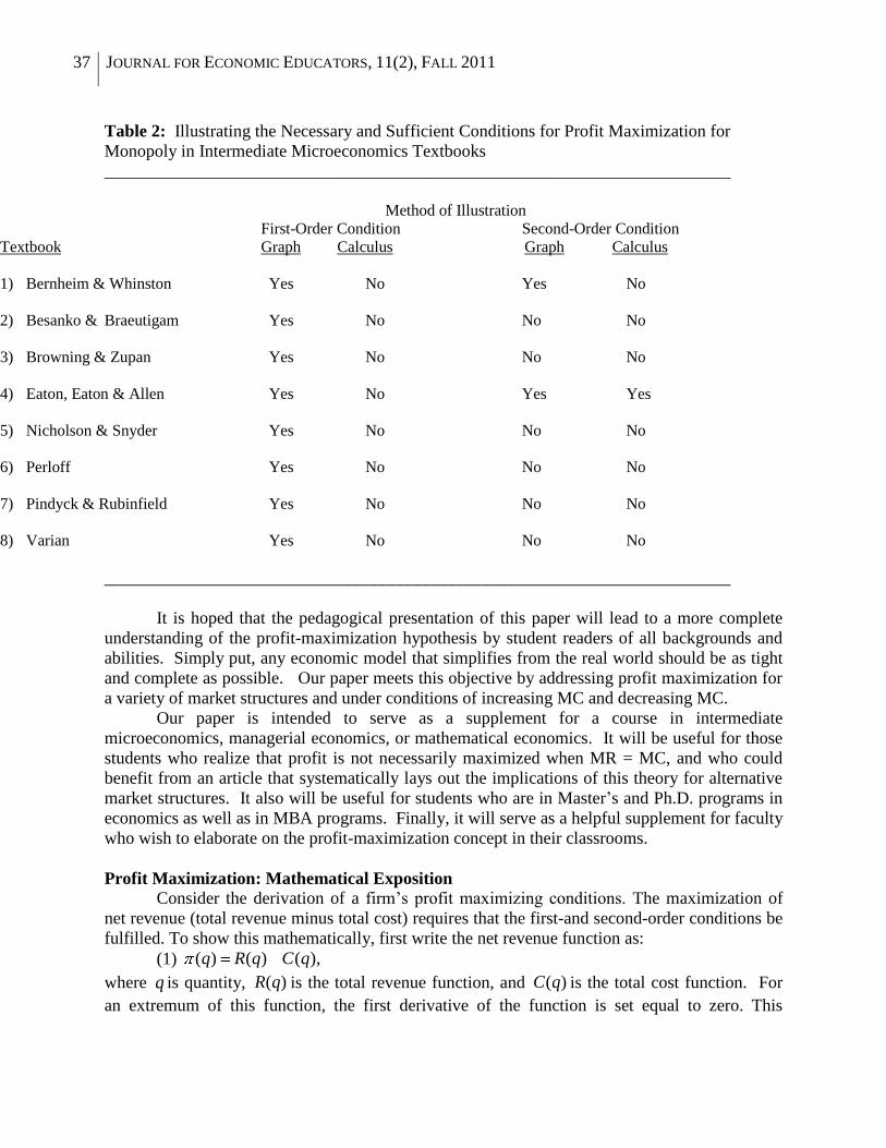
Table 2: Illustrating the Necessary and Sufficient Conditions for Profit Maximization for

Monopoly in Intermediate Microeconomics Textbooks

________________________________________________________________________

Method of Illustration

First-Order Condition Second-Order Condition

Textbook Graph Calculus Graph Calculus

1) Bernheim & Whinston Yes No Yes No

2) Besanko & Braeutigam Yes No No No

3) Browning & Zupan Yes No No No

4) Eaton, Eaton & Allen Yes No Yes Yes

5) Nicholson & Snyder Yes No No No

6) Perloff Yes No No No

7) Pindyck & Rubinfield Yes No No No

8) Varian Yes No No No

________________________________________________________________________

It is hoped that the pedagogical presentation of this paper will lead to a more complete

understanding of the profit-maximization hypothesis by student readers of all backgrounds and

abilities. Simply put, any economic model that simplifies from the real world should be as tight

and complete as possible. Our paper meets this objective by addressing profit maximization for

a variety of market structures and under conditions of increasing MC and decreasing MC.

Our paper is intended to serve as a supplement for a course in intermediate

microeconomics, managerial economics, or mathematical economics. It will be useful for those

students who realize that profit is not necessarily maximized when MR = MC, and who could

benefit from an article that systematically lays out the implications of this theory for alternative

market structures. It also will be useful for students who are in Master’s and Ph.D. programs in

economics as well as in MBA programs. Finally, it will serve as a helpful supplement for faculty

who wish to elaborate on the profit-maximization concept in their classrooms.

Profit Maximization: Mathematical Exposition

Consider the derivation of a firm’s profit maximizing conditions. The maximization of

net revenue (total revenue minus total cost) requires that the first-and second-order conditions be

fulfilled. To show this mathematically, first write the net revenue function as:

(1) ),()()( qCqRq

where q is quantity, )(qR is the total revenue function, and )(qC is the total cost function. For

an extremum of this function, the first derivative of the function is set equal to zero. This


suggests that the first-order condition is met--that marginal revenue equals marginal cost. This is

shown below as:

(2) 0)()(

q

qC

q

qR

q,

which implies,

(3) )()( qMCqMR .

That is, when marginal revenue and marginal cost are equal, the firm has either

maximized or minimized total profit. Using this reasoning, microeconomic texts suggest that

profit is maximized when marginal revenue equals marginal cost. Of course, for the extremum in

(2) to be a maximum (that is, profit maximization or loss minimization), the second-order

condition requires that the second derivative of the net revenue function have a negative value.

This is shown as:

(4) 0)()(

q

qMC

q

qMR,

or, adding q

qMC )(to both sides of the inequality,

(5)q

qMC

q

qMR )()(.

The net revenue function is at a maximum when the slope of the marginal cost curve,

q

qMC )(, exceeds that of the marginal revenue curve,

q

qMR )(.

Although calculus can be used to explain the first and second order conditions for profit

maximization, students often have difficulty in visualizing this method of presentation. Their

comprehension often improves when principles are illustrated in verbal and visual (graphical)

terms to which the rest of this paper is devoted.

Profit Maximization in Perfect Competition

It can also be shown graphically that the first-order condition of marginal revenue equals

marginal cost is a necessary, but not sufficient, condition for profit maximization. This is

presented here for the special case of perfect competition.

Because a perfectly competitive firm’s demand schedule is perfectly elastic, its marginal

revenue function is modeled as a horizontal line. Fulfillment of the general rule that the slope of

the marginal cost curve exceeds that of the marginal revenue curve necessarily requires that the

marginal cost curve have a positive slope at its point of intersection with the horizontal (zero

slope) marginal revenue curve.

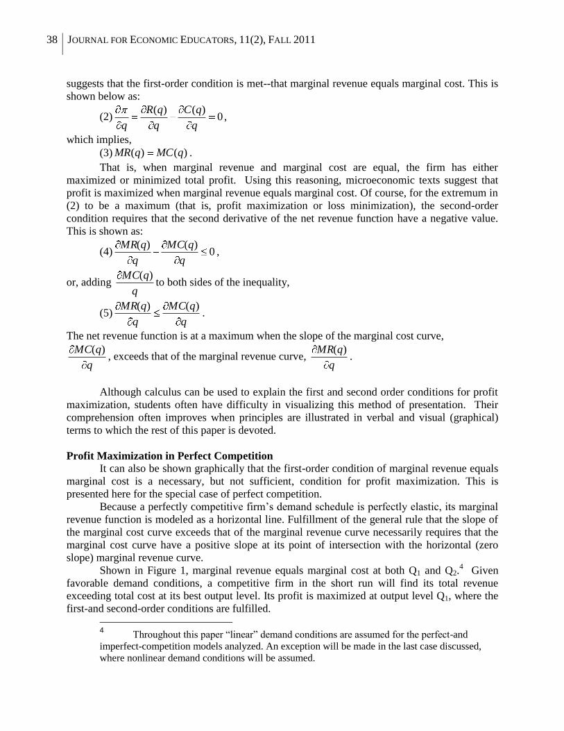
Shown in Figure 1, marginal revenue equals marginal cost at both Q1 and Q2.4 Given

favorable demand conditions, a competitive firm in the short run will find its total revenue

exceeding total cost at its best output level. Its profit is maximized at output level Q1, where the

first-and second-order conditions are fulfilled.

4 Throughout this paper “linear” demand conditions are assumed for the perfect-and

imperfect-competition models analyzed. An exception will be made in the last case discussed,

where nonlinear demand conditions will be assumed.


The minimization of net revenue (loss maximization) is not economically relevant given

the assumptions of rational seller behavior. Nevertheless, it can easily be shown given the

framework developed here. The two sufficient conditions for net revenue minimization are: (1)

the first-order condition: marginal revenue equals marginal cost; and (2) the second-order

condition: the slope of marginal revenue curve exceeds that of the marginal cost curve at their

point of intersection. In perfect competition, the second-order condition necessarily implies that

the marginal cost curve is decreasing (negative slope) at its point of intersection with the

horizontal (zero slope) marginal revenue curve. In Figure 1, net revenue minimization occurs at

Figure 1: Perfect Competition – Profit Maximization, Loss Minimization

at output level Q2, where the first-and second-order conditions are met.

5

5 The rationale of the second-order condition suggests the following. By increasing output

beyond Q1 more is added to total cost than to total revenue, since marginal cost exceeds marginal

revenue. Net revenue thus decreases. Similarly, by decreasing output below Q1 more is subtracted

from total revenue.


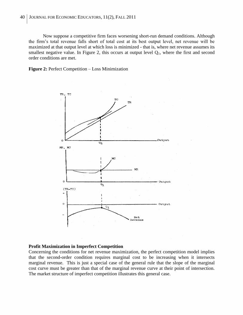
Now suppose a competitive firm faces worsening short-run demand conditions. Although

the firm’s total revenue falls short of total cost at its best output level, net revenue will be

maximized at that output level at which loss is minimized - that is, where net revenue assumes its

smallest negative value. In Figure 2, this occurs at output level Q1, where the first and second

order conditions are met.

Figure 2: Perfect Competition – Loss Minimization

Profit Maximization in Imperfect Competition

Concerning the conditions for net revenue maximization, the perfect competition model implies

that the second-order condition requires marginal cost to be increasing when it intersects

marginal revenue. This is just a special case of the general rule that the slope of the marginal

cost curve must be greater than that of the marginal revenue curve at their point of intersection.

The market structure of imperfect competition illustrates this general case.


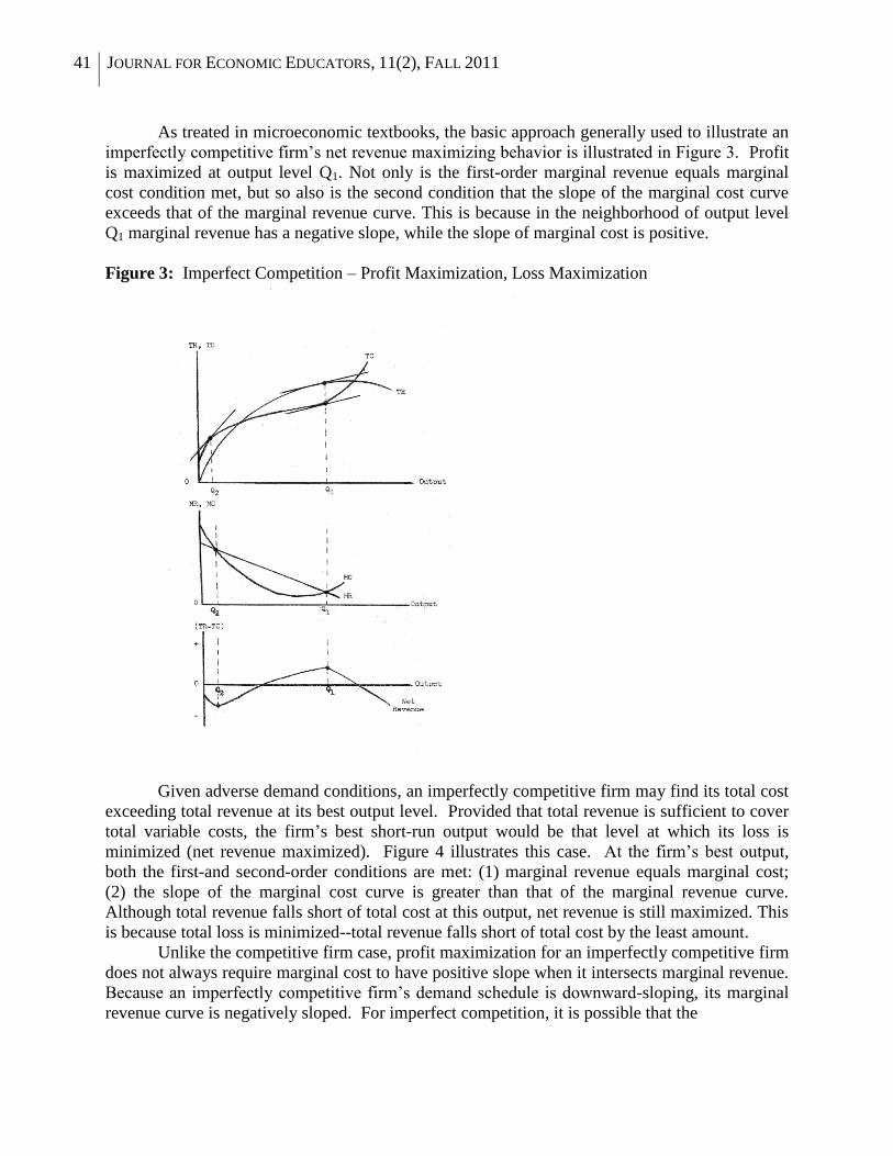
As treated in microeconomic textbooks, the basic approach generally used to illustrate an

imperfectly competitive firm’s net revenue maximizing behavior is illustrated in Figure 3. Profit

is maximized at output level Q1. Not only is the first-order marginal revenue equals marginal

cost condition met, but so also is the second condition that the slope of the marginal cost curve

exceeds that of the marginal revenue curve. This is because in the neighborhood of output level

Q1 marginal revenue has a negative slope, while the slope of marginal cost is positive.

Figure 3: Imperfect Competition – Profit Maximization, Loss Maximization

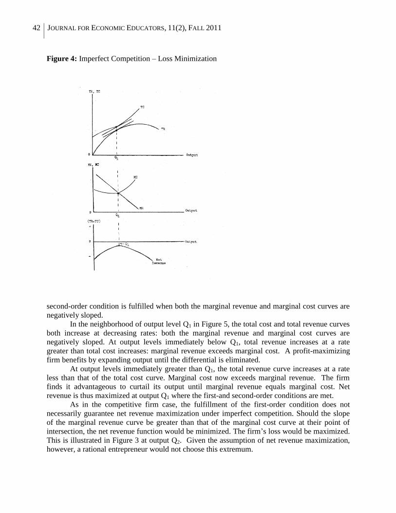
Given adverse demand conditions, an imperfectly competitive firm may find its total cost

exceeding total revenue at its best output level. Provided that total revenue is sufficient to cover

total variable costs, the firm’s best short-run output would be that level at which its loss is

minimized (net revenue maximized). Figure 4 illustrates this case. At the firm’s best output,

both the first-and second-order conditions are met: (1) marginal revenue equals marginal cost;

(2) the slope of the marginal cost curve is greater than that of the marginal revenue curve.

Although total revenue falls short of total cost at this output, net revenue is still maximized. This

is because total loss is minimized--total revenue falls short of total cost by the least amount.

Unlike the competitive firm case, profit maximization for an imperfectly competitive firm

does not always require marginal cost to have positive slope when it intersects marginal revenue.

Because an imperfectly competitive firm’s demand schedule is downward-sloping, its marginal

revenue curve is negatively sloped. For imperfect competition, it is possible that the


Figure 4: Imperfect Competition – Loss Minimization

second-order condition is fulfilled when both the marginal revenue and marginal cost curves are

negatively sloped.

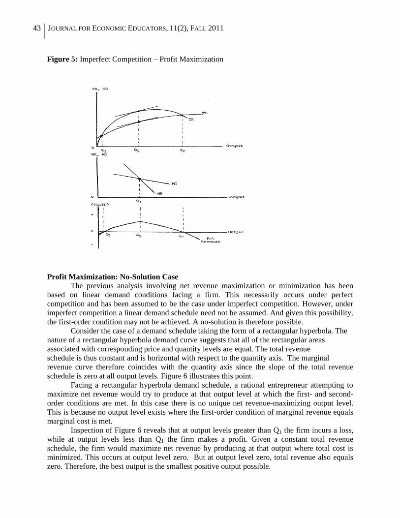
In the neighborhood of output level Q1 in Figure 5, the total cost and total revenue curves

both increase at decreasing rates: both the marginal revenue and marginal cost curves are

negatively sloped. At output levels immediately below Q1, total revenue increases at a rate

greater than total cost increases: marginal revenue exceeds marginal cost. A profit-maximizing

firm benefits by expanding output until the differential is eliminated.

At output levels immediately greater than Q1, the total revenue curve increases at a rate

less than that of the total cost curve. Marginal cost now exceeds marginal revenue. The firm

finds it advantageous to curtail its output until marginal revenue equals marginal cost. Net

revenue is thus maximized at output Q1 where the first-and second-order conditions are met.

As in the competitive firm case, the fulfillment of the first-order condition does not

necessarily guarantee net revenue maximization under imperfect competition. Should the slope

of the marginal revenue curve be greater than that of the marginal cost curve at their point of

intersection, the net revenue function would be minimized. The firm’s loss would be maximized.

This is illustrated in Figure 3 at output Q2. Given the assumption of net revenue maximization,

however, a rational entrepreneur would not choose this extremum.


Figure 5: Imperfect Competition – Profit Maximization

Profit Maximization: No-Solution Case

The previous analysis involving net revenue maximization or minimization has been

based on linear demand conditions facing a firm. This necessarily occurs under perfect

competition and has been assumed to be the case under imperfect competition. However, under

imperfect competition a linear demand schedule need not be assumed. And given this possibility,

the first-order condition may not be achieved. A no-solution is therefore possible.

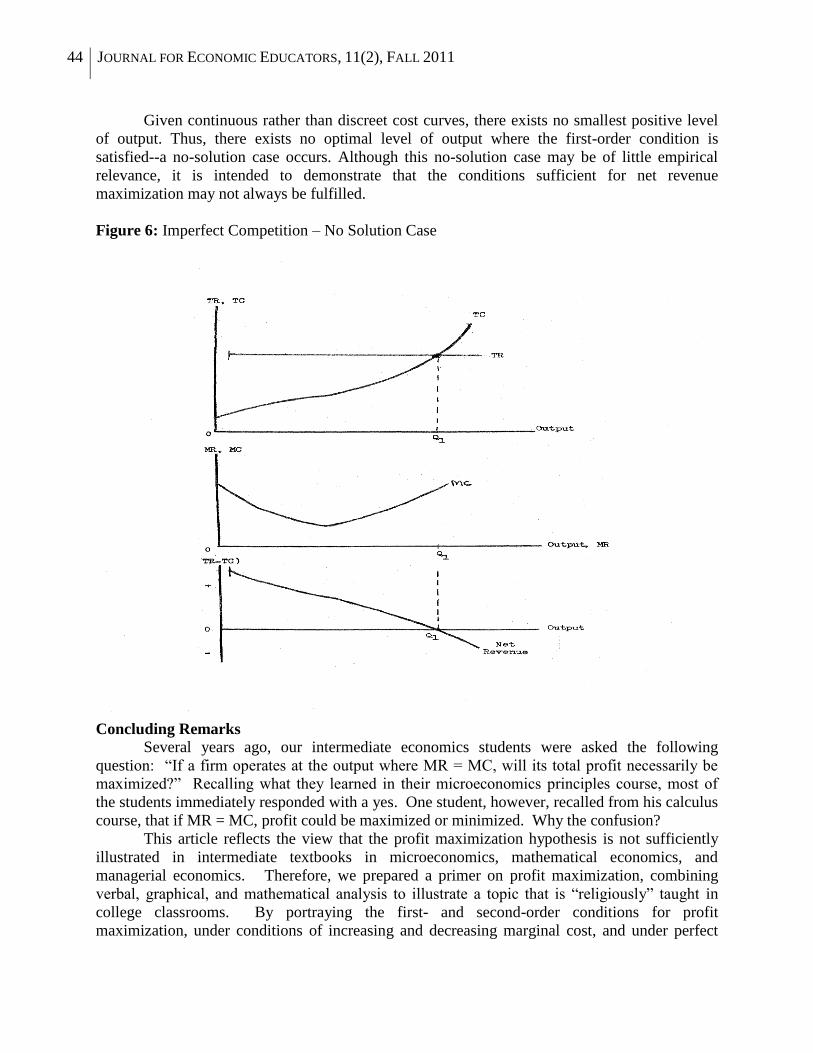
Consider the case of a demand schedule taking the form of a rectangular hyperbola. The

nature of a rectangular hyperbola demand curve suggests that all of the rectangular areas

associated with corresponding price and quantity levels are equal. The total revenue

schedule is thus constant and is horizontal with respect to the quantity axis. The marginal

revenue curve therefore coincides with the quantity axis since the slope of the total revenue

schedule is zero at all output levels. Figure 6 illustrates this point.

Facing a rectangular hyperbola demand schedule, a rational entrepreneur attempting to

maximize net revenue would try to produce at that output level at which the first- and second-

order conditions are met. In this case there is no unique net revenue-maximizing output level.

This is because no output level exists where the first-order condition of marginal revenue equals

marginal cost is met.

Inspection of Figure 6 reveals that at output levels greater than Q1 the firm incurs a loss,

while at output levels less than Q1 the firm makes a profit. Given a constant total revenue

schedule, the firm would maximize net revenue by producing at that output where total cost is

minimized. This occurs at output level zero. But at output level zero, total revenue also equals

zero. Therefore, the best output is the smallest positive output possible.


Given continuous rather than discreet cost curves, there exists no smallest positive level

of output. Thus, there exists no optimal level of output where the first-order condition is

satisfied--a no-solution case occurs. Although this no-solution case may be of little empirical

relevance, it is intended to demonstrate that the conditions sufficient for net revenue

maximization may not always be fulfilled.

Figure 6: Imperfect Competition – No Solution Case

Concluding Remarks

Several years ago, our intermediate economics students were asked the following

question: “If a firm operates at the output where MR = MC, will its total profit necessarily be

maximized?” Recalling what they learned in their microeconomics principles course, most of

the students immediately responded with a yes. One student, however, recalled from his calculus

course, that if MR = MC, profit could be maximized or minimized. Why the confusion?

This article reflects the view that the profit maximization hypothesis is not sufficiently

illustrated in intermediate textbooks in microeconomics, mathematical economics, and

managerial economics. Therefore, we prepared a primer on profit maximization, combining

verbal, graphical, and mathematical analysis to illustrate a topic that is “religiously” taught in

college classrooms. By portraying the first- and second-order conditions for profit

maximization, under conditions of increasing and decreasing marginal cost, and under perfect


competition and imperfect competition, this article attempts to provide a comprehensive

approach that clarifies this important concept.

This analysis is intended for the use of all students taking intermediate courses in

microeconomics, mathematical economics, and managerial economics. For those students in

graduate programs in economics and MBA programs, it serves as a helpful overview of

economic optimization. For instructors who wish to elaborate on the profit maximization

hypothesis beyond what is covered in textbooks, this article serves as a useful supplement.

References

Bernheim, Douglas and Michael Whinston, 2008. Microeconomics. McGraw-Hill/Irwin.

Besanko, David and Ronald Braeutigam. 2005. Microeconomics. John Wiley and Sons, Inc.

Browning, Edgar and Mark Zupan. 2009. Microeconomics: Theory and Applications. John

Wiley and Sons, Inc.

Case, Karl and Ray Fair. 2007. Principles of Microeconomics. Pearson/Prentice Hall.

Dadkhah, Kamran.2007. Foundations of Mathematical and Computational Economics.

Thomson/SouthWestern.

Dowling, Edward. 2001. Introduction to Mathematical Economics. Schaum’s Outlines/

McGraw-Hill.

Eaton, Curtis, Diane Eaton, and Douglas Allen. 2005. Microeconomics. Theory With

Applications. Pearson/ Prentice Hall.

Krugman, Paul and Robin Wells. 2009. Economics. Worth Publishers.

Mankiw, Gregory. 2009. Principles of Microeconomics. SouthWestern/ Cengage Learning.

Nicholson, Walter and Christopher Snyder. 2007. Intermediate Microeconomics and its

Applications. Thomson/ South-Western.

Perloff, Jeffery. 2009. Microeconomics. Pearson/Addison Wesley.

Pindyck, Robert and Daniel Rubinfeld. 2009. Microeconomics. Pearson/Prentice Hall.

Silberberg, Eugene and Wing Suen. 2001. The Structure of Economics: A Mathematical

Analysis. McGraw-Hill/Irwin.

Simon, Carl and Lawrence Blume. 1994. Mathematics for Economists. W. W. Norton &

Company. Sydsaeter, Knut and Peter Hammond.2006. Essential Mathematics for Economic Analysis.

Prentice Hall/Financial Times.

Documents

A Primer on Profit Maximization - ScholarWorks