A probabilistic approach for validation of advanced driver ...bdeschutter/pub/rep/04_016.pdf · ir. O.J. Gietelink ∗†, dr.ir. B. De ... ADAS typically consists of environment

Delft University of Technology

Delft Center for Systems and Control

Technical report 04-016

A probabilistic approach for validation of

advanced driver assistance systems∗

O.J. Gietelink, B. De Schutter, and M. Verhaegen

If you want to cite this report, please use the following reference instead:

O.J. Gietelink, B. De Schutter, and M. Verhaegen, “A probabilistic approach for

validation of advanced driver assistance systems,” Proceedings of the 8th TRAIL

Congress 2004 – A World of Transport, Infrastructure and Logistics – CD-ROM,

Rotterdam, The Netherlands, 17 pp., Nov. 2004.

Delft Center for Systems and Control

Delft University of Technology

Mekelweg 2, 2628 CD Delft

The Netherlands

phone: +31-15-278.51.19 (secretary)

fax: +31-15-278.66.79

URL: http://www.dcsc.tudelft.nl

∗This report can also be downloaded via http://pub.deschutter.info/abs/04_016.html

http://www.dcsc.tudelft.nl

http://pub.deschutter.info/abs/04_016.html

A probabilistic approach for validation of advanced driverassistance systems

TRAIL Research School, Delft, November 2004

Authorsir. O.J. Gietelink∗†, dr.ir. B. De Schutter∗, prof.dr.ir M. Verhaegen∗

∗ Delft University of Technology, Delft Center for Systems and Control† TNO Automotive

Contents

Abstract

1 Introduction . . . . . . . . . . . . . . . . . . . . . . . . . . . . . . . . . . . . . . . . . . . . . . . . . . . . . . . . . . . . . . . . 1

1.1 Advanced driver assistance systems . . . . . . . . . . . . . . . . . . . . . . . . . . . . . . . . . . . . . . . . 1

1.2 Objective of this paper . . . . . . . . . . . . . . . . . . . . . . . . . . . . . . . . . . . . . . . . . . . . . . . . . . . . . . 1

1.3 Outline of the paper . . . . . . . . . . . . . . . . . . . . . . . . . . . . . . . . . . . . . . . . . . . . . . . . . . . . . . . . . 2

2 A case study: Adaptive cruise control . . . . . . . . . . . . . . . . . . . . . . . . . . . . . . . . . . . 3

2.1 A simplified model and control law for adaptive cruise control . . . . . . . . . . 3

2.2 Performance criteria and perturbations for ACC . . . . . . . . . . . . . . . . . . . . . . . . . . 4

2.3 The control system validation problem. . . . . . . . . . . . . . . . . . . . . . . . . . . . . . . . . . . . . 4

3 A randomized algorithm for control system validation . . . . . . . . . . . . . . . . 6

3.1 Motivation for a probabilistic approach . . . . . . . . . . . . . . . . . . . . . . . . . . . . . . . . . . . . 6

3.2 Bounded sample complexity for RAs . . . . . . . . . . . . . . . . . . . . . . . . . . . . . . . . . . . . . . 6

3.3 Formulation of an RA . . . . . . . . . . . . . . . . . . . . . . . . . . . . . . . . . . . . . . . . . . . . . . . . . . . . . . . 7

3.4 Examples of application of an RA. . . . . . . . . . . . . . . . . . . . . . . . . . . . . . . . . . . . . . . . . . 8

3.4.1 Example 1: Uniformly distributed disturbance . . . . . . . . . . . . . . . . . . . . . . . . . . . . 8

3.4.2 Example 2: Gaussian Distributed Disturbance . . . . . . . . . . . . . . . . . . . . . . . . . . . . 10

3.4.3 Example 3: Multi-dimensional disturbance . . . . . . . . . . . . . . . . . . . . . . . . . . . . . . . . 10

3.5 Characteristics properties of RAs. . . . . . . . . . . . . . . . . . . . . . . . . . . . . . . . . . . . . . . . . . . 11

4 Reduction of the sample complexity . . . . . . . . . . . . . . . . . . . . . . . . . . . . . . . . . . . . . 12

4.1 A reduced worst-case bound . . . . . . . . . . . . . . . . . . . . . . . . . . . . . . . . . . . . . . . . . . . . . . . . 12

4.2 Reduction of the sampling space . . . . . . . . . . . . . . . . . . . . . . . . . . . . . . . . . . . . . . . . . . . 12

4.3 Importance sampling . . . . . . . . . . . . . . . . . . . . . . . . . . . . . . . . . . . . . . . . . . . . . . . . . . . . . . . . 13

5 Methodological approach . . . . . . . . . . . . . . . . . . . . . . . . . . . . . . . . . . . . . . . . . . . . . . . . . 14

5.1 Specification . . . . . . . . . . . . . . . . . . . . . . . . . . . . . . . . . . . . . . . . . . . . . . . . . . . . . . . . . . . . . . . . . 14

5.2 Simulation . . . . . . . . . . . . . . . . . . . . . . . . . . . . . . . . . . . . . . . . . . . . . . . . . . . . . . . . . . . . . . . . . . . 14

5.3 Model validation . . . . . . . . . . . . . . . . . . . . . . . . . . . . . . . . . . . . . . . . . . . . . . . . . . . . . . . . . . . . 14

5.4 Performance measure . . . . . . . . . . . . . . . . . . . . . . . . . . . . . . . . . . . . . . . . . . . . . . . . . . . . . . . 15

6 Conclusions . . . . . . . . . . . . . . . . . . . . . . . . . . . . . . . . . . . . . . . . . . . . . . . . . . . . . . . . . . . . . . . . . 16

Acknowledgments . . . . . . . . . . . . . . . . . . . . . . . . . . . . . . . . . . . . . . . . . . . . . . . . . . . . . . . . . . . . . . . . . . . . . . . 17

References . . . . . . . . . . . . . . . . . . . . . . . . . . . . . . . . . . . . . . . . . . . . . . . . . . . . . . . . . . . . . . . . . . . . . . . . . . . . . . . . 18

Abstract

This paper presents a methodological approach for validation of advanced driver assis-

tance systems. The methodology relies on the use of randomized algorithms that are

more efficient than conventional validation using simulations and field tests, especially

with increasing complexity of the system. The methodology consists of first specifying

the perturbation space and performance criteria. Then a minimum number of samples

and a relevant sampling space is selected. Next an iterative randomized simulation is

executed, followed by validation of the simulation model by hardware tests, in order

to increase the reliability of the estimated performance. The concept is illustrated with

some examples of a case study involving an adaptive cruise control system. The case

study also points out some characteristic properties of randomized algorithms regard-

ing the necessary sample complexity, and the sensitivity to model uncertainty. Solutions

for these issues are proposed as well as corresponding recommendations for future re-

search.

Keywords

Advanced driver assistance systems, intelligent vehicles, controller validation, random-

ized algorithms, adaptive cruise control

A probabilistic approach for validation of advanced driver assistance systems 1

1 Introduction

1.1 Advanced driver assistance systems

The increasing demand for safer passenger vehicles has stimulated the research and de-

velopment of advanced driver assistance systems (ADASs) over the past decade. An

ADAS typically consists of environment sensors (e.g. radar, laser, and vision sensors)

and electronic control functions to improve driving comfort and traffic safety by warn-

ing the driver, or even autonomous control of actuators. State-of-the-art examples of

ADASs that have already been introduced by the automotive industry are adaptive cruise

control (ACC), collision warning systems, and pre-crash systems.

The demand for safety and reliability naturally increases with the increasing au-

tomation of the vehicle’s driving task, since the driver must fully rely on flawless op-

eration of the ADAS. E.g., autonomous braking in an ACC should be executed only

if the distance to the preceding vehicle will otherwise become unacceptably small, or

even result in a collision. In order to handle a large variety of complex traffic scenarios

and disturbances, redundancy and fault-tolerance measures are often implemented. In

practice, it is however difficult to choose the right control measures and to validate their

effectiveness. Manufacturers thus face an increasing effort in the design and validation

of ADASs in contrast to a desired shorter time-to-market.

Currently, an iterative process of simulations and prototype test drives on a test track

is used for validation purposes. The simulation effort can however be unreliable due to

model uncertainty, and inefficient, since a large number of simulations are necessary to

achieve a representative result. Instead, a worst-case analysis is often used, which leads

to a conservative control system design, thus limiting the functional performance of the

ADAS. On the other hand, test drives are more reliable, but can never cover the entire

set of operating conditions, due to time and cost constraints. Furthermore, test results

can be difficult to analyze for controller validation and benchmarking, because traffic

scenarios cannot be exactly reproduced during a test drive. It may therefore become

impossible to evaluate an ADAS with guaranteed measures for the level of performance,

safety, and reliability.

1.2 Objective of this paper

The objective of this paper is to present a methodological approach based on random-

ized algorithms (RAs) to provide an efficient test program in order to cover the entire set

of operating conditions with a minimum number of samples. A simplified case study

will be used as an illustration of this methodology for reasons of transparency. Note

that the emphasis of this paper is therefore on the validation process, and not on control

system design.

One validation tool in this methodology is the software tool PRESCAN, which is

used in a probabilistic simulation strategy with the operating conditions chosen to be

representative for the ‘real’ conditions. The simulation models can subsequently be val-

idated with another tool: the VEhicle-Hardware-In-the-Loop (VEHIL) facility, TNO’s

tailor-made laboratory for testing ADASs. In VEHIL a real ADAS equipped vehicle is

tested in a hardware-in-the-loop simulation, as shown by the working principle in Fig-

ure 1. With VEHIL the development process and more specifically the validation phase

of ADASs can be carried out safer, cheaper, more manageable, and more reliable. Both

2 TRAIL Research School, Delft, November 2004

��

(equipped with ADAS)Vehicle Under Test

meter

Chassis

Absolute

parameters

Simulator (MARS)

Multi−Agent Real−Time

parameters

Relative

Moving Base

traffic participant)

vehicle obstacle

Vehicle Model

Dynamo−

(representing other

Figure 1: VEHIL working principle.

VEHIL and PRESCAN are fully described by Gietelink et al. (2004), and in this paper

we restrict the discussion to the underlying validation methodology, as outlined below.

1.3 Outline of the paper

This paper is organized as follows. In Section 2 a simplified model of an ACC system is

presented, together with its performance measures and the perturbations acting on the

system. Section 3 treats the background theory of RAs that is subsequently applied to

the ACC case study in a number of examples. These examples illustrate the advantages

of using RAs, but also highlight some points for improvement, especially regarding the

required number of samples. Section 4 discusses some possibilities for addressing this

issue. Subsequently, Section 5 presents an improved methodological approach for the

validation of ADASs. This methodology consists of first specifying the perturbation

space and performance criteria. Then a minimum number of samples and a relevant

sampling space is selected, using the reduction techniques from Section 4. Next an

iterative randomized simulation is executed, followed by validation of the simulation

model by hardware tests in the VEHIL facility, in order to increase the reliability of

the estimated performance. Finally, Section 6 summarizes the validation approach, and

discusses ongoing research activities. The added value of this paper is to connect the

research areas of ADASs, RAs, and conventional methods for control system validation.


2 A case study: Adaptive cruise control

2.1 A simplified model and control law for adaptive cruise control

Figure 2 illustrates an ACC-equipped vehicle following a lead vehicle, with their po-

sition x and velocity v, where the subscripts ‘l’ and ‘f’ denote leader and follower re-

spectively. Further defined are the distance between the two vehicles (the headway)

xr = xl − xf, the relative velocity vr = vl − vf, the desired distance xd, and the headway

separation error ex = xd − xr.

xr

vfvl

xdex

driving directionleading vehicle following vehicle

Figure 2: Two vehicles in ACC mode: one leader and one follower.

ACC tries to maintain a pre-defined velocity set-point vcc, unless a slower vehicle

is detected ahead. In that case vehicle ‘f’ is controlled to follow vehicle ’l’ with equal

velocity vf = vl at a desired distance xd. Since the ACC objective is to control the motion

of a vehicle relative to a preceding vehicle, the vehicle state is chosen as x=[

xr vr

]T.

We can describe the evolution of the systems by

x =

[

0 1

0 0

][

xr

vr

]

+

[

0

−1

]

af +

[

0

1

]

al, (1)

where the acceleration of the following vehicle af is the input to the system, and the

leading vehicle al the disturbance. The initial condition x(0) =[

xr, 0 vr, 0

]Tis deter-

mined and set as soon as the sensor detects a new lead vehicle that ACC should follow.

In distance control mode, ad is given by proportional feedback control of the dis-

tance separation error ex = xd − xr and its derivative ev = ex = vd − vr

ad =−k2ev − k1ex, k1, k2 > 0. (2)

The distance xd and the feedback gains ki are tuning parameters. In this paper we use a

constant spacing control law, where xd is equal to a constant value s0 = 40m, k1 = 1.2,

and k2 = 1.7. Since the desired relative velocity is obviously equal to zero, (2) can be

rewritten as

ad = k2vr + k1(xr − s0). (3)

This control law is asymptotically stable, so that both ex en ev are always regulated

to zero, provided k1, k2 > 0 (Swaroop, 1994). In this paper we also neglect sensor

processing delay and vehicle dynamics by assuming that the desired acceleration is

realized at the input of the controlled system without any time lag, such that u = ad.

However, we do introduce an actuator saturation, since ACC systems usually restrict

the minimum and maximum control input u for safety reasons. In this case study we

use the restriction that af is bounded between -2.5 and 2.5 m/s2.


2.2 Performance criteria and perturbations for ACC

The performance of an ACC can be quantified in a number of measures ρi, e.g. over-

shoot, tracking error, time response, control effort, ride comfort, and string stability.

Here we restrict the controller validation to the measure of safety, expressed as the

probability p that no collision will occur for a whole range of traffic situations. The

safety measure for a single experiment is denoted by ρs ∈ {0,1}, where ρs = 1 means

that the ACC system manages to follow the preceding vehicle at a safe distance, and

ρs = 0 means that the traffic scenario would require a brake intervention by the driver

to prevent a collision1. Depending on the resulting value for p, the feedback gains

k1 and k2 can be optimized. In practice, it is not desirable to achieve p = 1 for all

traffic scenarios, since this would necessitate a very conservative controller with high

autonomous braking capacity. ACC field test results suggest that p = 0.95 is more or

less appropriate for highway cruising (Fancher et al., 1998).

The value of ρs for a particular traffic scenario obviously depends on the pertur-

bations imposed by that scenario. The disturbance to the ACC system is formed by

the motion of other vehicles that are detected by the environment sensors. Apart from

the acceleration of the preceding vehicle al, also the initial conditions x(0) determine

the probability of a collision. These scenario parameters, together with measurement

noise, process noise, unmodelled dynamics and various types of faults construct an n-

dimensional perturbation space ∆. It is then of interest to evaluate the function ρ∆

that reflects the dependency of ρ on the structure of this complex and probably non-

convex space ∆. In reality the perturbation space is constructed by dozens of param-

eters (including sensor characteristics, driver behavior, and vehicle dynamics). In this

paper we restrict the validation to ∆ being limited to the subset S = {al, xr, 0, vr, 0} of

uncertain traffic scenario parameters and where the resulting safety measure ρs(∆) is

non-decreasing.

2.3 The control system validation problem

Designing a simple stable controller that meets the ACC performance requirements is

not difficult. However, validation of this controller with respect to these requirements

and subsequent tuning may require a lot of effort. For low-order systems, controller

validation can still be solved in a deterministic way or by using iterative algorithms. But

when the dimension of ∆ increases and ρ(∆) becomes non-convex, it can be expected

that the problem will become more difficult to solve, and eventually become intractable,

as shown in the tutorial paper by Vidyasagar (1998).

Currently, controller validation is therefore often performed by a grid search, where

all parameters are varied through their operating range (see, e.g., Fielding et al. (2002)).

However, such a validation strategy is not very efficient, since an exhaustive grid search

may require a very large number of experiments, perhaps even too large to be feasible.

Alternatively, a worst-case analysis can be performed by lumping together a combina-

tion of disturbances, each with the direction and magnitude that has the worst impact on

the system performance ρ . Such a worst-case analysis on a control system is however

unrealistic, since it may result in a conservative controller that is tuned to a specific

non-reachable combination of operating conditions. In the next sections we therefore

1Please note the difference between the performance level ρ for a particular experiment and its prob-

ability p for a whole range of experiments.


discuss and further extend an approach to address this problem.


3 A randomized algorithm for control system valida-

tion

3.1 Motivation for a probabilistic approach

An alternative approach for solving a complex problem exactly, is to solve it approxi-

mately by using a randomized algorithm (RA). An RA makes random choices during its

execution, and covers both Monte Carlo, sequential and other probabilistic algorithms

(Motwani, 1995). The use of an RA can turn an intractable problem into a tractable one,

but at the cost that the algorithm may fail to give a correct solution (without the user

knowing). The probability that the RA fails can be made arbitrarily close to zero, but

never exactly equal to zero. A popular example is a Monte Carlo simulation strategy,

where this probability depends on the sample complexity, i.e. the number of simulations

performed. An important issue is therefore the necessary sample complexity that guar-

antees a certain level of confidence for the simulation outcome. In this section we show

that this sample complexity is bounded, depending on the desired level of accuracy and

reliability, but also that these bounds are rather conservative.

3.2 Bounded sample complexity for RAs

The use of a randomized approach for controller validation can be illustrated as follows.

Consider an arbitrary process with only two possible outcomes: ‘failure’ (ρ = 0) and

‘success’ (ρ = 1). Suppose that we wish to determine the probability p for a successful

outcome of this process. If N denotes the number of experiments with this process and

NS the number of experiments with successful results, then the ratio NS/N is called the

empirical probability or empirical mean pN for a successful result of the process.

However, pN is unlikely to be exactly equal to the real probability p, although it is

reasonable to expect that pN will approach p, as N → ∞, and as long as the samples

are chosen to be representative of the set ∆. The question thus arises in what sense pN

converges to p, and how many experiments N have to be performed to give a reason-

able estimate of p. An estimate pN can be called reasonable if it differs from the real

(unknown) value p by no more than ε > 0, such that

|p− pN | ≤ ε, (4)

where ε is called the accuracy of the estimate.

Since pN is a random variable depending on the particular realization of the N sam-

ples, the inequality (4) is only valid with a certain probability of realization. Therefore,

we cannot always guarantee that |p− pN | ≤ ε , even with a large number of experiments.

This means that if the experiments are performed another N times, the estimate pN will

probably have another value. The probability that |p− pN j| > ε for a particular set of

simulations N j is then the unreliability δ of the estimate pN . We would therefore like

to know the level of accuracy ε , and reliability 1−δ , that can be obtained with one par-

ticular set of N simulations. In practice, often the reverse problem is considered: how

many experiments N are necessary to achieve a desired level of confidence, in terms of

ε and δ?

To answer this question, first define the desired accuracy for determining the un-

known quantity p by some number ε > 0. Then, in order to know the reliability of

our set of experiments, it is necessary to determine the probability that performing N


Table 1: Values for ε , δ , Nch, and Nwc, according to the Chernoff bound (5) and the

worst-case bound (10).

δ ε Nch Nwc

0.10 0.10 150 22

0.05 0.10 185 29

0.03 0.10 210 34

0.02 0.10 231 38

0.01 0.10 265 44

0.002 0.10 346 59

δ ε Nch Nwc

0.05 0.05 738 59

0.02 0.05 922 77

0.01 0.05 1060 90

0.02 0.03 2559 129

0.01 0.01 26492 459

0.001 0.001 3800452 6905

experiments will generate an estimate pN for which |p− pN |> ε . The Chernoff bound

(Chernoff, 1952) states that this probability, defined as δ > 0, is no larger than 2e−2Nε2.

This means that, after performing the experiment N times, we can state with a confi-

dence of at least 1−2e−2Nε2that the empirical probability pN is no more than ε different

from the true but unknown probability p. So, in order to estimate the unknown quantity

p to an accuracy of ε and with a confidence of 1− δ , the number of experiments N

should be chosen such that 2e−2Nε2≤ δ , or equivalently

Nch ≥1

2ε2ln

2

δ, (5)

which is known as the additive Chernoff bound. Table 1 presents the necessary sample

complexity to calculate pN for some values of ε and δ . Since pN has a confidence

interval, the upper bound for N is called a soft bound, as opposed to hard bounds given

by a deterministic algorithm.

3.3 Formulation of an RA

The Chernoff bound forms the basis for the application of Monte Carlo methods, used

widely in engineering for design and analysis of control system performance. Several

references give a clear tutorial introduction to the use of RAs (Alippi, 2002; Calafiore

et al., 2003; Tempo et al., 2004; Vidyasagar, 1998). Here we summarize the main steps

to be taken in control system analysis using RAs.

Suppose that the closed-loop system (in our case the ACC equipped vehicle and its

controller) must be verified for a certain performance level ρ . It is then the goal to

estimate the probability p that this performance ρ lies above a pre-specified threshold

value γ . In order to compute2 pN(γ), we generate N independent identically distributed

(iid) samples ∆1,∆2, . . . ,∆N in the perturbation space ∆ according to its probability den-

sity function (pdf) f∆(∆). The outcome of every i-th experiment is represented by an

indicator function J, given by

J(∆i) =

{

0, if ρ < γ1, if ρ ≥ γ

(6)

The empirical probability pN can then be estimated as

pN =1

N

N

∑i=1

J(∆i), (7)

2In the following we will also use pN instead of pN(γ) for reasons of clarity.


which is known as the simple sampling estimator. Since the outcome of the inequal-

ity |p− pN | ≤ ε is a random variable, it has a certain probability of realization. By

introducing a confidence degree 1−δ , this probability is defined as

Pr{|p(γ)− pN(γ)| ≤ ε} ≥ 1−δ , ∀ γ ≥ 0, δ ∈ (0,1), ε ∈ (0,1) (8)

The sample complexity N that is required for (8) to hold, can then be calculated from

(5). This method for probabilistic control system analysis is formalized as follows:

Algorithm 3.1 (Probabilistic performance verification (Tempo et al., 2004))

Given ε > 0, δ ∈ (0,1) and γ ≥ 0, this RA returns with probability at least 1−δan estimate pN(γ) for the probability p(γ), such that |p(γ)− pN(γ)| ≤ ε .

1. Determine the necessary sample size N = Nch ≥1

2ε2ln

2

δ;

2. Draw N samples ∆1, . . . ,∆N according to f∆;

3. Return the empirical probability pN(γ) =1

N

N

∑i=1

J(

∆(i))

where J (·) is the

indicator function of the set B = {∆ : ρ (∆)≥ γ}.

3.4 Examples of application of an RA

In this section we will apply Algorithm 3.1 to the simplified ACC case study, of which

the ‘true’ outcome is exactly known. If we are interested in knowing the number of

traffic situations that would become dangerous, given a stochastic distribution of traffic

scenarios, we can use Algorithm 3.1 to give an estimate pN of this probability p with

an accuracy level ε and a confidence level δ , based on N simulations.

3.4.1 Example 1: Uniformly distributed disturbance

Scenario definition In this first example we choose a highway cruising scenario

where the lead vehicle approaches a traffic jam and brakes to a full stop. The initial

conditions are xr,0 = xd = 40m, and vl(0) = vf(0) = 30 m/s. We assume that the de-

celeration of the preceding vehicle is the only disturbance with a uniform distribution

between −10 and 0 m/s2, denoted as f U(al) ∼ U [−10, 0]. We also restrict the anal-

ysis to the measure of safety ρs. In situations when the lead vehicle brakes hard, the

ACC vehicle cannot obtain the necessary deceleration ad, since the actuator saturates

at -2.5 m/s2. Now, for fine-tuning the controller parameters, we would like to know the

percentage of brake situations for which ρs meets a pre-defined threshold. The threshold

γ is simply set at 1 in this case (no collision).

The safety of the system obviously decreases with a stronger deceleration al, such

that the function ρs(al) is non-decreasing. Therefore, the boundary value ∆γ , for which

only just a collision is prevented, can easily be calculated using an iterative algorithm

as −3.015m/s2. Below this value the scenario will always result in a collision, above

this value the ACC vehicle will be able to stop autonomously and prevent a collision.

Since al is uniformly distributed on the interval [−10, 0], the real value for p is thus

equal to (3.015/10) = 0.3015. The probability that the estimated value pN differs from

this real value by an accuracy ε is then 1−δ , as defined by (8).


0.1 0.15 0.2 0.25 0.3 0.35 0.4 0.45 0.50

10

20

30

40

50

60

Histogram of 500 simulation sets, with N = 100 eachUniform distribution of acceleration profile

Num

ber

of sim

ula

tion s

ets

pN j

(a) Histogram of 500 simulation sets, with N = 100

each, where al ∼ U (−10,0).

0.9 0.92 0.94 0.96 0.98 10

20

40

60

80

100

120

140

Histogram of 500 simulation sets, with N = 100 each Gaussian distribution of acceleration profile

Num

ber

of sim

ula

tion s

ets

pN j

(b) Histogram of 500 simulation sets, with N =100 each, where the acceleration profile is sampled

from a Gaussian distribution N (0,1.5).

0.7 0.75 0.8 0.85 0.9 0.95 1 1.050

10

20

30

40

50

60

70

Histogram of 500 simulation sets, with N = 100 eachDisturbances of a

l, v

r and x

r

Num

ber

of sim

ula

tion s

ets

pN j

(c) Histogram of 500 simulation sets, with N =100 each, with a multi-dimensional disturbance for

S = {vl, vf, xr, al}.

Figure 3: Histograms for the estimate pN j.

Randomization of the problem Although for this example it is feasible to formulate

a deterministic algorithm, in practice it can be difficult or even impossible to determine

p in a deterministic way, when the dimension of ∆ increases and the relation ρ(∆)becomes non-convex. So instead of calculating p explicitly in deterministic sense, the

function is randomized in such a way that it takes a random input ∆i from its distribution

function f U(al), according to Algorithm 3.1.

In order to verify the performance of Algorithm 3.1, we execute it 500 times (each

with N = 100). So every j-th simulation set, for j = 1, . . . ,500, gives us an estimate

pN j. The distribution of the estimate is shown in the histogram in Figure 3(a). With

this example, the accuracy and reliability for a single simulation set (each consisting

of 100 simulations), can be estimated as ε and δ respectively. The empirical mean pM

of the probability of a collision-free scenario is 0.30714, based on all MN = 50000

simulations, which is very close to p = 0.3015, as could be expected. The variance of

each individual estimate pN jcan be found by the unbiased estimator for the variance

σ2N j−1 =

1

N j −1∑

N j

j=1(pN j

− pM), which gives σ2N j−1 = 0.0021042.

Analysis of the simulation results Suppose we desire that δ = 0.10 and ε = 0.10; (5)

then gives Nch = 150 as an upper bound on the sample complexity. The desired values


for δ and ε imply that the empirical mean pN jfor the j-th set of simulations should lie in

[0.2015,0.4015] for every 9 out 10 simulation sets. However, from Figure 3(a) we ob-

serve that in total only 15 out of the 500 simulation sets result in pN j/∈ [0.2015,0.4015].

So δ is empirically determined at δ = 15/500 = 0.03, which is smaller than the desired

δ . The estimate pN jfor any simulation set j is thus more reliable than desired, and we

only used 100 experiments, whereas (5) requires Nch = 150.

This example suggests that a certain value for δ and ε can be achieved with a lower

number of samples than deemed necessary by the Chernoff bound. Correspondingly, by

choosing N = Nch, a higher level of accuracy and reliability can be obtained. Although

the degree of conservatism for this example is rather limited, it can be shown that this

conservatism increases with smaller values for δ and ε (Vidyasagar, 1998).

3.4.2 Example 2: Gaussian Distributed Disturbance

In the previous example, f U(al) may not be representative for the entire operating range,

whereas pN greatly depends on the correctness of the underlying pdf. Let us therefore

assume a more general acceleration profile for highway cruising. Typical vehicle mea-

surements during ACC field testing (Fancher et al. (1998)) suggest that the acceleration

profile can be roughly described as a random signal with a Gaussian distribution f N

with mean µ = 0 and standard deviation σ = 1.5, denoted as N (0,1.5), truncated on

the interval [−10,10] m/s2.

We now execute Algorithm 3.1 again with al ∼ N (0,1.5). Figure 3(b) shows the

resulting histogram with the estimated collision probability pN jfor every simulation

set is shown. The empirical mean pM is now 0.97752, with a variance of σ2N j−1 =

0.00020506, which is much smaller than in Example 1, due to the lower occurrence

rate of dangerous situations.

Suppose that δ = 0.02 and ε = 0.03 are desired; (5) then gives Nch = 2559. From

Figure 3(b) we see that only 10 out of 500 estimates pN jfall outside the interval [p−

ε, p+ ε], which gives an estimated reliability δ = 0.02. So the same level of accuracy

and reliability has been achieved with only N = 100 instead of Nch = 2559 samples.

3.4.3 Example 3: Multi-dimensional disturbance

In the previous two examples al was considered the only disturbance. However, in

practice p depends also on the initial distance and velocities of both vehicles at the

moment of first detection by the sensor. Consider for instance a cut-in situation at

close distance xr, which is more dangerous than a vehicle cutting-in at larger distance

(with identical al and vr). The crash probability thus depends on the entire set S ={vl, vf, xr, al} that defines the longitudinal scenario, as discussed in Section 2.2. In this

example we assume Gaussian distributions for both the velocities (with µ = 30 m/s and

σ = 5 m/s), and distance xr (with µ = 60 m, σ = 20 m, and truncated on [10,150]m).

Figure 3(c) shows the resulting histogram after execution of Algorithm 3.1 with

pM = 0.86848 and σ2N j−1 = 0.0010378. Compared to Example 2 it can be seen that

the variance is much larger, since the outcome of the experiment now depends on four

independent pdfs. The sample complexity N is again conservative, since Figure 3(c)

shows that only one estimate falls outside the interval [p− ε, p+ ε], indicating δ =0.002. So the same level of accuracy and reliability has been achieved with only N =100 instead of Nch = 346 samples.


3.5 Characteristics properties of RAs

The examples and key references (Alippi, 2002; Calafiore et al., 2003; Tempo et al.,

2004; Vidyasagar, 1998) point out the following characteristic properties:

• A limited number of test runs is necessary as compared to deterministic algo-

rithms. However, the sample complexity to achieve a reasonable ε and δ , as

given by the Chernoff bound, is quite conservative.

• An RA is very simple, since the Chernoff bound is completely independent of the

nature of the underlying process and the perturbation space ∆. However, this also

means that no advantage is taken of any a priori knowledge of the structure of ∆.

It is therefore desired to modify the simulation approach such that knowledge of

the system is applied.

• The reliability of the simulation outcome strongly depends on the reliability of the

pre-defined pdf f∆. The outcome of the simulation approach also greatly depends

on the modeling effort.

• The empirical mean pN does not say anything about the minimum or maximum

level of performance that can be expected. It may well be that a control system

has a good average performance, but also a poor worst-case performance.

In the next section methods used in conventional control system validation will be ap-

plied to address these issues. These methods will be integrated with the RA approach,

and illustrated with the ACC case study. The resulting methodology will be presented

in Section 5.


4 Reduction of the sample complexity

As mentioned in the previous section, the sample complexity N given by the Chernoff

bound is too conservative. Reduction of N for ADAS validation is therefore an impor-

tant challenge. One way is to reformulate the problem and use a different test objective.

In addition, the sampling space ∆ can be reduced by neglecting certain subsets that are

impossible to occur. Subsequently, N can be further reduced by using a priori knowl-

edge on which samples will be more interesting than others. These reduction techniques

are also valid for conventional validation techniques, but are now integrated with the RA

approach.

4.1 A reduced worst-case bound

The examples in Section 3 were based on estimation of the mean performance p. Alter-

natively, we can estimate the worst-case performance ρmax by ρN = maxi=1,2,...,N ρ(∆i).Tempo et al. (1997) prove that the minimum number of samples N which guarantees

that

Pr{Pr{ρ (∆)> ρN} ≤ ε} ≥ 1−δ (9)

is then given by

N ≥ln1/δ

ln1/(1− ε). (10)

The sample complexity given by (10) is much lower than for (5), as shown in Table 1,

and is more suitable in case of a worst-case analysis.

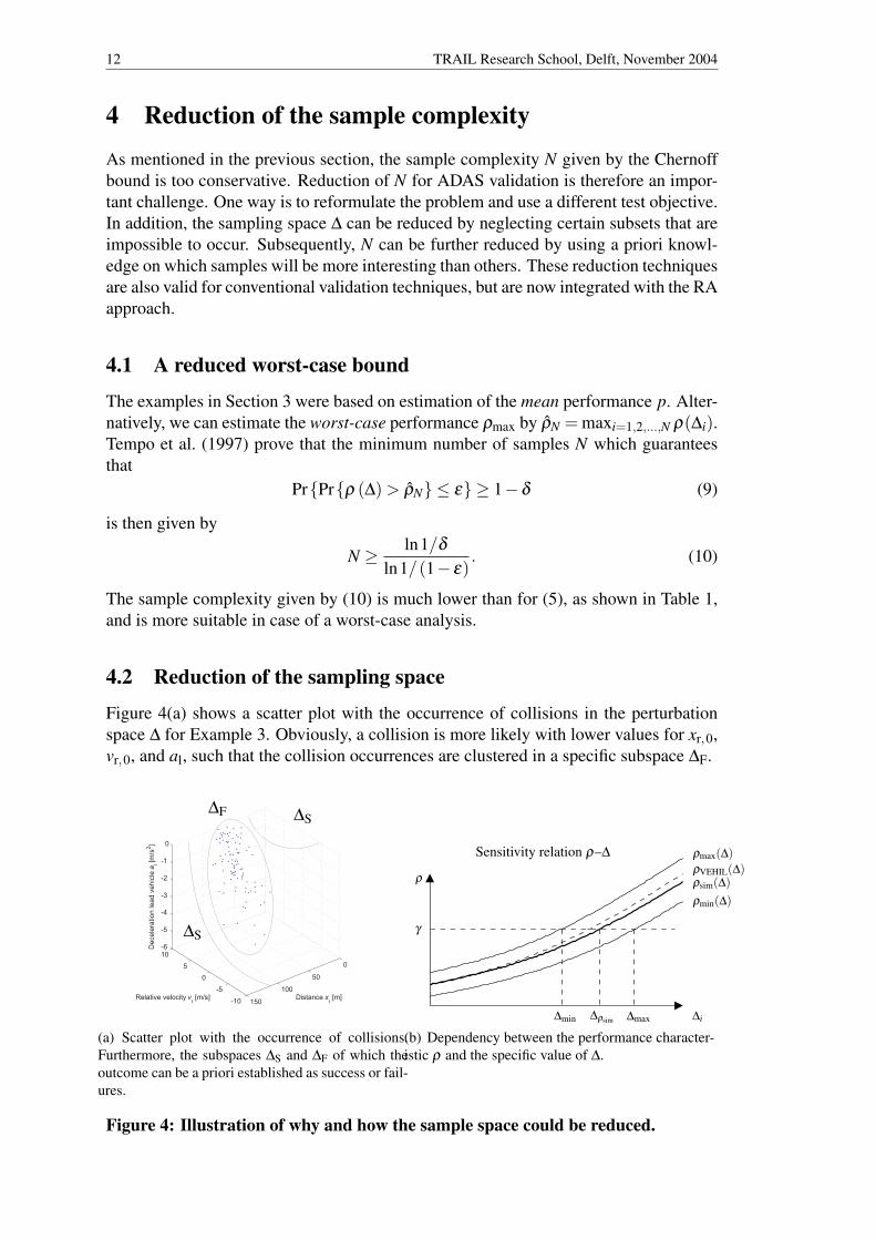
4.2 Reduction of the sampling space

Figure 4(a) shows a scatter plot with the occurrence of collisions in the perturbation

space ∆ for Example 3. Obviously, a collision is more likely with lower values for xr,0,

vr,0, and al, such that the collision occurrences are clustered in a specific subspace ∆F.

∆S

∆S∆F

(a) Scatter plot with the occurrence of collisions.

Furthermore, the subspaces ∆S and ∆F of which the

outcome can be a priori established as success or fail-

ures.

γ

ρ

Sensitivity relation ρ–∆

∆i∆min ∆ρsim ∆max

ρmax(∆)

ρVEHIL(∆)ρsim(∆)

ρmin(∆)

(b) Dependency between the performance character-

istic ρ and the specific value of ∆.

Figure 4: Illustration of why and how the sample space could be reduced.


This means that there is structure in the perturbation space ∆ and in the function

ρ(∆) that can be used to reduce the necessary perturbation space of interest. The sam-

pling space can then be reduced by disregarding specific subsets of ∆, of which the

outcome is a priori known. An example is the subset ∆S with combinations of positive

acceleration and positive relative velocity that will never result in a potential collision.

When this dependency ρ(∆) can be proven to be convex or non-decreasing, the

sample complexity N can be significantly reduced, as illustrated in Figure 4(b). In this

case an RA can iteratively search for the boundary value ρ(∆γ) = γ , and neglect any ∆i

larger than ∆γ , since the outcome of those samples can be predicted in advance.

4.3 Importance sampling

As stated above, it makes sense to give more attention to operating conditions that are

more likely to cause a collision than others.

Suppose that we want to estimate a probability p, given a perturbation ∆. If f∆ is a

pdf ∼ U [0,1] on the interval S = [0,1], our goal is then to estimate

p =∫

SJ(∆) f∆(∆)d∆ = E[J(∆)] (11)

where J is the performance function, and ∆ ∼ f∆. Importance sampling is a sampling

technique to increase the number of occurrences of the event of which the probability

p should be estimated (Madras, 2002). This estimation is corrected by dividing it by

the increased probability of the occurrence of the event. In order to highlight the inter-

esting subset ∆F it thus makes sense not to sample from the original pdf f∆, but instead

use an artificial pdf, reflecting the importance of the events, and then reweighing the

observations to get an unbiased estimate.

We can now define an importance sampling pdf ϕ that is strictly positive on S. We

can then write

p =∫

S

(

J(∆) f∆(∆)

ϕ(∆)

)

ϕ(∆)d∆ = E

[

J(Φ) f∆(Φ)

ϕ(Φ)

]

, (12)

where Φ ∼ ϕ . The importance sampling estimator based on ϕ is

p[ϕ]N =1

N

N

∑i=1

J(Φi) f∆(Φi)

ϕ(Φi)(13)

where Φ1, . . . ,ΦN are iid with pdf ϕ . Its variance is

var( p [ϕ]N) =1

N

[

∫

S

J(∆)2 f∆(∆)2

ϕ(∆)d∆− p2

]

(14)

An efficient estimator p[ϕ]N is obtained by choosing ϕ proportional to the ‘impor-

tance’ of the individual samples, where importance is defined as |J(∆) f∆(∆)|. A rare but

dangerous event can thus be equally important as a more frequent but less dangerous

event.


5 Methodological approach

A major problem with ADAS controller validation is that the system cannot be tested ex-

haustively for every disturbance under every operating condition. A validation method-

ology should therefore provide a suitable test program in order to sufficiently (but

also efficiently) cover the entire perturbation space. To this aim we propose a generic

methodological approach, consisting of the steps described in the following sections.

5.1 Specification

Firstly, define performance measures ρ and corresponding evaluation criterion γ . In

addition, the desired δ and ε must be defined. Correspondingly, select the test objective

in order to determine the type of bound for N:

• Probability of performance satisfaction: for a given δ , ε , check if the perfor-

mance measure ρ is below threshold γ with a certain probability level p for the

whole perturbation space ∆.

• Worst-case performance: check if the worst-case performance ρmax is within ε of

ρN with a certain probability 1−δ .

Then, identify the perturbation space ∆ and its pdf f∆ by using preliminary field

test results. Using knowledge on the structure of ∆ or the function ρ(∆), determine

subsets ∆F and ∆S, of which the outcome is a priori known (either failure or success).

Furthermore, a simulation model of the vehicle, its sensor system, and its control system

is designed using the dedicated simulation tool PRESCAN (Labibes et al. (2003)).

5.2 Simulation

Then execute an RA using importance sampling (cf. Section 4.3) to cover the important

part of the perturbation space to estimate the performance pN with respect to the criteria

defined earlier. In general ρ can be a continuous value, although we used a discrete

value in the examples.

The performance of an RA using importance sampling depends heavily on the re-

liability of the models and the pdfs used in the simulation phase. The robustness of

pN to model uncertainty should therefore be considered when validating an ADAS in a

randomized approach. The experimental relation between ρ and ∆ from the simulations

is then bounded between ρmax and ρmin, as illustrated in Figure 4(b). This means that

the estimated boundary value lies within the interval [∆min, ∆max], provided that ρ(∆)is a non-decreasing relation.

5.3 Model validation

Therefore, the most interesting samples of the perturbation space ∆i are chosen to be

reproduced in the VEHIL facility, also in a randomized approach to efficiently cover

∆. These particular ∆i are selected to lie within the interval [∆min, ∆max]. In VEHIL

disturbances can be introduced in a controlled and accurate way, thereby achieving a

more reliable estimate than ρsim(∆). In this way the model uncertainty can be reduced,


because of the replacement of a vehicle and sensor model by real hardware. The corre-

sponding test program can be formalized as follows:

Algorithm 5.1 (Probabilistic model validation)

1. Choose initial values for ∆min and ∆max in accordance with the uncertainty

size, and a suitable N.

2. Test ρ at ∆min

3. IF ρ ≥ γ , THEN decrease ∆min and GOTO 2.

IF ρ < γ , THEN decrease ∆max and GOTO 4.

4. Test ρ at ∆max

5. IF ρ ≥ γ , THEN increase ∆min and GOTO 2.

IF ρ < γ , THEN increase ∆max and GOTO 4.

6. Return the empirical probability

pN =1

N

N

∑i=1

J(

∆(i))

The sample complexity N for VEHIL is calculated as follows. Suppose that the

requirement is that ρ ≤ γ , where γ is a small number, and we want to determine N

in the case that all tests have been successful, i.e. pN = 1. Then we want to check if

Pr{| pN − p| ≤ ε} ≥ 1−δ , where ε is set equal to γ . From ε and the desired confidence

level δ , the necessary number N can then be derived with the Chernoff bound.

Apart from obtaining ρVEHIL, the test results can also be used for model validation.

The estimate pN may indicate necessary improvements in the system design regard-

ing fine-tuning of the controller parameters. Improve the simulation model using the

VEHIL test results until the simulation model proves to provide adequate performance,

convergence in pN and sufficient samples N.

5.4 Performance measure

In an iterative process the simulation results in step 5.2 and thus the estimate pN can be

improved. Subsequently, the VEHIL test program in step 5.3 can be better optimized

by choosing a smaller interval [∆min, ∆max]. From the combination of simulation and

VEHIL results the performance pN of the ADAS can then be estimated with a high level

of reliability, and the controller design can be improved. Finally, determine ρVEHIL with

(13), correcting it for the higher occurrence rate in the interval [∆min, ∆max].


6 Conclusions

We have presented a methodological approach for probabilistic performance validation

of advanced driver assistance systems, and applied a randomized algorithm (RA) to a

simple adaptive cruise control problem. This probabilistic approach cannot prove that

the system is safe or reliable. However, we accept a certain risk of failure (though

small), since any other conventional validation process (e.g. test drives) is also based

on a probabilistic analysis. Furthermore, use can be made of a priori information on the

system, thereby emphasizing interesting samples.

Ongoing research is focused on extension of this methodological approach to more

complex ADAS models, with non-convex performance functions ρ∆ and multiple per-

formance criteria (safety, stability, and driving comfort). Furthermore, model validation

will be performed using a real hardware setup in the VEHIL facility.


Acknowledgments

Research supported by TNO Automotive, TRAIL Research School, and the TU Delft

spearhead program “Transport Research Centre Delft: Towards Reliable Mobility”.


References

Alippi, C. (2002) Randomized algorithms: A system-level, poly-time analysis of robust compu-

tation, IEEE Trans. on Computers, 51(7), pp. 740–749.

Calafiore, G., F. Dabbene, R. Tempo (2003) Randomized algorithms in robust control, in: Proc.

of the 42nd IEEE Conference on Decision and Control, Maui, Hawaii, USA, pp. 1908–1913.

Chernoff, H. (1952) A measure of asymptotic efficiency for tests of a hypothesis based on the

sum of observations, Annals of Mathematical Statistics, 23, pp. 493–507.

Fancher, P., R. Ervin, J. Sayer, M. Hagan, S. Bogard, Z. Bareket, M. Mefford, J. Haugen (1998)

Intelligent cruise control field operational test, Tech. Rep. DOT HS 808 849, DOT/National

Highway Traffic Safety Administration, final report.

Fielding, C., A. Vargas, S. Bennani, M. Selier, eds. (2002) Advanced Techniques for Clearance

of Flight Control Laws, Springer, Berlin, Germany.

Gietelink, O., D. Verburg, K. Labibes, A. Oostendorp (2004) Pre-crash system validation with

PRESCAN and VEHIL, in: Proc. of the IEEE Intelligent Vehicles Symposium (IV), Parma, Italy.

Labibes, K., Z. Papp, A. Thean, P. Lemmen, M. Dorrepaal, F. Leneman (2003) An integrated

design and validation environment for intelligent vehicle safety systems (IVSS), in: Proc. of the

10th World Congress on Intelligent Transport Systems and Services (ITS), Madrid, Spain, paper

2731.

Madras, N. (2002) Lectures on Monte Carlo Methods, American Mathematical Society, Provi-

dence, Rhode Island, USA.

Motwani, R. (1995) Randomized Algorithms, Cambridge University Press, New York.

Swaroop, D. (1994) String Stability of Interconnected Systems: An Application to Platooning in

Automated Highway Systems, Ph.D. thesis, University of California at Berkeley.

Tempo, R., E. Bai, F. Dabbene (1997) Probabilistic robustness analysis: Explicit bounds for the

minimum number of samples, Systems & Control Letters, 30, pp. 237–242.

Tempo, R., G. Calafiore, F. Dabbene (2004) Randomized Algorithms for Analysis and Control

of Uncertain Systems, Springer-Verlag, Berlin, Germany.

Vidyasagar, M. (1998) Statistical learning theory and randomized algorithms for control, IEEE

Control Systems Magazine, 18(6), pp. 69–85.

Documents

A probabilistic approach for validation of advanced driver ...bdeschutter/pub/rep/04_016.pdf · ir. O.J. Gietelink ∗†, dr.ir. B. De ... ADAS typically consists of environment