i

A PROBABILISTIC CONCEPTUAL DESIGN AND SIZING

APPROACH FOR A HELICOPTER

A THESIS SUBMITTED TO

THE GRADUATE SCHOOL OF NATURAL AND APPLIED SCIENCES

OF

MIDDLE EAST TECHNICAL UNIVERSITY

BY

SELİM SELVİ

IN PARTIAL FULFILLMENT OF THE REQUIREMENTS

FOR

THE DEGREE OF MASTER OF SCIENCE

IN

AEROSPACE ENGINEERING

SEPTEMBER 2010

ii

Approval of the thesis:

A PROBABILISTIC CONCEPTUAL DESIGN AND SIZING APPROACH

FOR A HELICOPTER

submitted by SELİM SELVİ in partial fulfillment of the requirements for the degree

of Master of Science in Aerospace Engineering Department, Middle East

Technical University by,

Prof. Dr. Canan Özgen _____________________

Dean, Graduate School of Natural and Applied Sciences

Prof. Dr. Ozan Tekinalp _____________________

Head of Department, Aerospace Engineering

Asst. Prof. Dr. İlkay Yavrucuk _____________________

Supervisor, Aerospace Engineering Dept., METU

Examining Committee Members:

Prof. Dr. Serkan Özgen _____________________

Aerospace Engineering Dept., METU

Asst. Prof. Dr. İlkay Yavrucuk _____________________

Aerospace Engineering Dept., METU

Assoc. Prof. Dr. Funda Kurtuluş _____________________

Aerospace Engineering Dept., METU

Asst. Prof. Dr. Oğuz Uzol _____________________

Aerospace Engineering Dept., METU

Dr. Osman Merttopçuoğlu _____________________

Chief Engineer, ROKETSAN

Date: 15.09.2010

iii

I hereby declare that all information in this document has been obtained and

presented in accordance with academic rules and ethical conduct. I also declare

that, as required by these rules and conduct, I have fully cited and referenced

all material and results that are not original to this work.

Name, Last name : Selim Selvi

Signature :

iv

ABSTRACT

A PROBABILISTIC CONCEPTUAL DESIGN AND SIZING APPROACH FOR A

HELICOPTER

Selvi, Selim

M.Sc. Department of Aerospace Engineering

Supervisor : Asst. Prof. Dr. İlkay Yavrucuk

September 2010, 62 Pages

Due to its complex and multidisciplinary nature, the conceptual design phase of

helicopters becomes critical in meeting customer satisfaction. Statistical

(probabilistic) design methods can be employed to understand the design better and

target a design with lower variability. In this thesis, a conceptual design and

helicopter sizing methodology is developed and shown on a helicopter design for

Turkey.

Keywords: Helicopter, Conceptual Design, QFD, OEC, RF-Method, Response

Surface, Probabilistic Design, Sensitivity and Monte Carlo Analysis

v

ÖZ

BİR HELİKOPTER İÇİN PROBABİLİSTİK KAVRAMSAL TASARIM VE

BOYUTLANDIRMA YAKLAŞIMI

Selvi, Selim

Yüksek Lisans, Havacılık ve Uzay Mühendisliği Bölümü

Tez Yöneticisi : Yrd. Doç. Dr. İlkay Yavrucuk

Eylül 2010, 62 Sayfa

Helikopter tasarımının karmaşık ve çok-disiplinli doğası gereği, kavramsal tasarım

sürecindeki boyutlandırma çalışmasının müşteri memnuniyeti için başarım seviyesi

büyük önem taşır. Böyle karmaşık bir sistemin çok-disiplinli analizi yoğun çalışma

ve uzun zaman gerektirir. Tasarım için gereken bu sürenin kısaltılması için

istatistiksel (olasılıksal) tasarım metodları kullanılabilir. Bu tez çalışmasında,

Türkiye ihtiyaçlarına uygun bir helikopterin kavramsal boyutlandırılması, çok-

disiplinli ve olasılıksal bir tasarım yaklaşımı ile yapıldı.

Anahtar Kelimeler: Helikopter, Kavramsal Tasarım, QFD, OEC, RF-Metodu,

Response Surface, Olasılıksal Tasarım, Hassasiyet ve Monte Carlo Analizi

vi

To My Family,

vii

ACKNOWLEDGMENT

I wish to express his gratitude to my supervisor Asst. Prof. Dr. İlkay YAVRUCUK

for his guidance, advice, criticism, encouragements and insight throughout the

research.

I also would like to address my deepest thanks to my family for their endless support

during this study and throughout my life.

Finally, the assistance of anyone who has a contribution somehow is gratefully

acknowledged.

viii

TABLE OF CONTENTS

ABSTRACT ................................................................................................................ iv

ÖZ ................................................................................................................................ v

ACKNOWLEDGMENT ............................................................................................ vii

TABLE OF CONTENTS .......................................................................................... viii

LIST OF TABLES ....................................................................................................... x

LIST OF FIGURES .................................................................................................... xi

LIST OF SYMBOLS AND ABBREVIATIONS ..................................................... xiii

1 INTRODUCTION ................................................................................................ 1

1.1 Problem Statement ................................................................................... 1

1.2 Literature Survey ...................................................................................... 1

1.3 Motivation and Contributions of This Thesis .......................................... 3

1.4 Thesis Outline .......................................................................................... 3

2 THEORITICAL PRELIMINARIES ..................................................................... 4

2.1 Quality Functional Deployment Analysis ................................................ 4

2.2 Selection of Helicopter Configuration ..................................................... 6

2.2.1 Fuel Fraction (RF) Method Based Sizing and Overall Evaluation

Criteria .......................................................................................................... 7

2.3 Parameter Sensitivity Analysis .............................................................. 11

2.3.1 Design of Experiment (DOE) ........................................................ 12

2.3.2 Response Surface (RS) Analysis .................................................... 13

2.3.3 Monte Carlo Simulations ............................................................... 17

2.4 Conseptual Sizing of Main Components of Helicopter ........................ 17

2.4.1 Component Weights ....................................................................... 17

2.4.2 Dimension Characteristics ............................................................. 19

ix

3 CONCEPTUAL SIZING AND ANALYSIS ...................................................... 20

3.1 Design Requirements ............................................................................. 22

3.2 Competitor Study ................................................................................... 23

3.3 Quality Functional Deployment Analysis .............................................. 24

3.4 Selection of Helicopter Configuration ................................................... 27

3.4.1 Helicopter Preliminary Sizing Using OEC and RF-Optimization . 27

3.4.2 DOE & Response Surface (RS) Analysis ...................................... 29

3.4.3 Monte Carlo Analysis .................................................................... 43

3.4.4 Analysis for Forward Flight Performance ..................................... 51

3.5 Weight and Dimension Estimations ....................................................... 52

3.5.1 Weights .......................................................................................... 52

3.5.2 Dimensions and Configuration Layout .......................................... 53

4 CONCLUSIONS ................................................................................................. 54

REFERENCES ........................................................................................................... 57

APPENDIX ............................................................................................................... 59

A. DESCRIPTIONS AND DEFINITIONS FOR THE QFD DESIGN TOOL..59

x

LIST OF TABLES

TABLES

Table 3.1 Mission Profile Segments .......................................................................... 23

Table 3.2 Competitor Helicopters‟ Specifications ..................................................... 24

Table 3.3 First Fifteen Configurations in terms of OEC Score ................................. 29

Table 3.4 CASE1 BB Design Variables .................................................................... 31

Table 3.5 CASE2 BB Design Variables .................................................................... 37

Table 3.6 RSE Coefficients ........................................................................................ 43

Table 3.7 Monte Carlo Parameters ............................................................................ 44

Table 3.8 Calculated size of main components of helicopter .................................. 53

Table 3.9 Dimensions of Selected Configuration ...................................................... 53

Table 4.1 Comparison with the competitor helicopters ............................................. 55

xi

LIST OF FIGURES

FIGURES

Figure 2.1 Configuration Selection and Evaluation Method ....................................... 6

Figure 2.2 RF Method [10] .......................................................................................... 8

Figure 2.3 Sensitivity Analysis Method ..................................................................... 11

Figure 2.4 BB Design Points ...................................................................................... 13

Figure 2.5 Pareto Plot [4] ........................................................................................... 15

Figure 2.6 Actual by Predicted Plot [5] ..................................................................... 16

Figure 2.7 Prediction Profiler [6] ............................................................................... 16

Figure 3.1 Flowchart of the Design Method .............................................................. 20

Figure 3.2 Reference Mission Profile ........................................................................ 22

Figure 3.3 QFD Matrix .............................................................................................. 25

Figure 3.4 OEC Variation .......................................................................................... 28

Figure 3.5 Pareto Plot for Gweight Response for CASE1 ......................................... 32

Figure 3.6 Pareto Plot for Horse Power Response for CASE1 .................................. 33

Figure 3.7 Pareto Plot for Evaluation Score Response for CASE1 ........................... 33

Figure 3.8 Summary of Fits for CASE1 .................................................................... 34

Figure 3.9 CASE1 2nd Order Fit for Gross Weight Response .................................. 34

Figure 3.10 CASE1 2nd

Order Fit For Horse power................................................... 35

Figure 3.11 CASE1 2nd

Order Fit for Evaluation Score............................................. 35

Figure 3.12 Prediction Profiler for CASE1 ................................................................ 36

Figure 3.13 Pareto Plot for Gweight Response for CASE2 ....................................... 38

Figure 3.14 Pareto Plot for Horse Power Response for CASE2 ................................ 39

Figure 3.15 Pareto Plot for Evaluation Score Response for CASE2 ......................... 39

xii

Figure 3.16 Summary of Fits for CASE2.................................................................. 40

Figure 3.17 CASE2 2nd

Order Fit For Gross Weight ................................................. 40

Figure 3.18 CASE2 2nd

Order Fit For Horse Power .................................................. 41

Figure 3.19 CASE2 2nd

Order Fit For Evaluation Score ............................................ 41

Figure 3.20 Prediction Profiler for CASE2 ................................................................ 42

Figure 3.21 Distribution of Variables (a, b, c, d) ....................................................... 45

Figure 3.22 Monte Carlo Results ............................................................................... 47

Figure 3.23 OEC PDF distributions (a, b, c, d) .......................................................... 47

Figure 3.24 MC results when all variables changed .................................................. 50

Figure 3.25 PDF distribution when all variables changed ......................................... 50

Figure 3.26 Example gross weight estimation for AS350 3B .................................... 51

Figure 3.27 Gross weight estimation for selected configuration ............................... 52

Figure A.1 Example QFD Matrix .............................................................................. 60

xiii

LIST OF SYMBOLS AND ABBREVIATIONS

Symbol Definition Unit

C Specific Fuel Consumption lb/hp/lb

W Weight lb

WG Gross Weight lb

WU Useful Load lb

Φ Empty to Gross Weight Ratio -

R Main Rotor Radius ft

Vc Cruise Velocity knot

P Power hp

ω Angular velocity rad/s

σ Disk Loading -

AR Range Parameter -

AT Hover Parameter -

K Weight Correction Factor -

LF Fuselage Length ft

LT2M Distance Between Tail And Main Rotors ft

RTR Tail Rotor Radius ft

LCl Clearance Length ft

LTOTAL Total Length ft

Abbreviation Definition

RSE Response Surface Equation

RF Fuel Fraction

AHS American Helicopter Society

xiv

BB Box Behnken

OEC Overall Evaluation Criteria

CCD Central Composite Design

QFD Quality Functional Deployment

HOT Higher Order Terms

SFC Specific Fuel Consumption

P/W Power to Weight Ratio

MTBF Mean Time Between Failure

MTTR Mean Time to Repair

HOQ House of Quality

TR Tail Rotor

DS Drive Shaft

LG Landing Gear

FC Flight Control

RPM Revolution Per Minute

1

CHAPTER 1

1 INTRODUCTION

1.1 Problem Statement

Modern aircraft design is a multidisciplinary design problem with many

contradicting decisions to make. In the conceptual design phase, the designers have

more freedom to make design changes and the most influential design choices are

made in this phase. Yet, this is the design phase where the least about the problem is

known. On the other hand, it is desired to obtain more and more information about

the system at its early design phases. In this thesis, probability based design methods

are employed to target customer satisfaction. Consequently, a conceptual helicopter

design and sizing suitable for the Turkish market is used as a case study.

1.2 Literature Survey

In this section a literature survey on helicopter design is presented. The main

concentration of this survey is on the conceptual design of rotary wing aircrafts,

implementation of the concurrent engineering tools such as Quality Functional

Deployment (QFD) and Overall Evaluation Criteria (OEC), and probabilistic design

methods such as Response Surface Methodology and Monte Carlo Analysis.

The theoretical background on helicopter rotor hub design can be found in Ref. [1].

Specifically, the selection and sizing procedures of rotor hubs are given in detail in

2

this reference. Similarly, the detailed information on the preliminary design of

helicopters is illustrated in Ref. [10]. This handbook covers almost all aspects of

helicopter preliminary design. It includes the methods for the selection of

configurations (Chapter 3 of [10]).

Lecture notes of Schrage, D.P on Rotorcraft Systems Design [2] present analytical

design methods which prevent the need for trial and error. In this reference,

simultaneous solutions to both weight and aerodynamic performances of helicopters

are presented. Thus, this paper is the main source to utilize the Fuel Fraction (RF)

method and sizing of the helicopter.

In 2006, a short course on Response Surface Methodology was hold by Mavris, D.

N. at Middle East Technical University (METU) in Ankara. Application of Response

Surface Methodology on aircraft preliminary design was introduced in this course.

References [4] and [5] belong to the course material and were quite helpful for the

generation of the Response Surface Equations for the conceptual design. Also, the

implementations of Design of Experiments and Response Surface Method (RSM)

with JMP (a statistical design tool) are illustrated in these references.

A study on “System Synthesis In Preliminary Aircraft Design Using Statistical

Methods” had been presented at the 20th Congress of the International Council of the

Aeronautical Sciences DeLaurentis, D., Mavris, D. N. and Schrage, D.P. in 1996 [3].

In this study, an approach to conceptual and early preliminary aircraft design is

documented. System synthesis is accomplished using statistical methods, such as

Design of Experiments (DOE) and Response Surface Methodology (RSM). A

systematical implementation of DOE, RSM and QFD tools on an air vehicle

preliminary design work can be found in this paper.

Another study was carried out by Frits, A. P., Fleeman, E. L. and Mavris, D. N.

named as “Use of a Conceptual Sizing Tool for Conceptual Design of Tactical

Missiles” [6]. Together with Ref. [3], assistance of the methodology introduced in

this paper played a significant role in implementation of statistical methods in this

thesis.

In 2006 the Metucopter Design Team entered the American Helicopter Society‟s

helicopter graduate design competition. The design report [7] presents a helicopter

3

design procedure with the use of concurrent engineering tools. This report was

employed as a guide especially in construction of the QFD matrix and

implementation of OEC.

A study was conducted by Vikhansky A., Kraft M. at 2003 regarding Monte Carlo

Methods for Identification and Sensitivity Analysis of Coagulation Processes [8],.

Although, the area of implementation is quite different, this paper led the way in

application of Monte Carlo method for sensitivity analysis.

Ref. [11] presents the main construction and evaluation steps of Monte Carlo

Analysis.

The thesis required the search for helicopters for a similar class. Thus a search was

conducted to find similar helicopters and their specifications. The two helicopters of

Eurocopter Company were selected as competitors and the specifications were found

in companies‟ official site [9].

1.3 Motivation and Contributions of This Thesis

The motivation of this thesis is to accomplish a conceptual design and sizing

approach of a civilian helicopter suitable for the Turkish Market and to provide a

basis for a conceptual system design with the implementation of multidisciplinary

and probabilistic design approaches in the conceptual sizing of a helicopter.

1.4 Thesis Outline

In Chapter 1, first the problem is introduced and then, a literature survey is provided.

Chapter 2 gives the theoretical background on the multidisciplinary and probabilistic

design methods employed in the conceptual sizing process.

Chapter 3 presents the conceptual design, analysis procedure and results.

Chapter 4 discusses the analysis results and presents the conclusions.

4

CHAPTER 2

2 THEORITICAL PRELIMINARIES

In this section, the theoretical background of the methods utilized in this thesis is

presented. First, the Quality Functional Deployment (QFD) analysis method is

introduced. This method enables the designer to relate the customer requirements to

engineering parameters. Then, a method of helicopter configuration selection is

explained. In that part, preliminaries for Fuel Fraction (RF) (for hover and forward

flight) and Overall Evaluation Criteria (OEC) methods are given in details. Next,

the methodology of the parameter sensitivity analysis is defined. Finally, some

empirical formulas for conceptual helicopter sizing are illustrated. These equations

are to be employed in the determination of the size of main helicopter components.

2.1 Quality Functional Deployment Analysis

In classical helicopter design some of the driving design parameters are disk loading,

solidity, tip speed and empty weight,. Although those parameters are significant for

all helicopters, the most important design variables may change according to

customer needs, type of the helicopter or mission profile. In order to account for this

fact and to find out the most important design variables a QFD method is employed

in this thesis.

In this method, helicopter sizing, a large scale problem, is defined as one that

possesses both high dimensionality and multi-objective attributes. The design of a

5

complex vehicle such as helicopter requires analysis across multiple disciplines.

Some of these disciplines might have competing objectives. As a result, the designer

usually has control over many input variables and wants to track how each variable

affects the responses to determine what trade-offs are needed to be made. When the

number of design variables coming into play is increased, the dimensionality of the

design space grows, and more sample design points are required to explore the entire

region in all dimensions.

The QFD matrix is employed to discover the most important design drivers by

relating the customer requirements to engineering parameters through the decision

matrix („whats‟ vs. „hows‟). This method also allows the designer to find out the real

most important design variables regardless of what the traditional methods say.

In this method, each customer requirement is given a weighted importance level

between 1 (least important) and 5 (most important). Then, for several sections of the

helicopter design discipline (aerodynamics, structure, propulsion, control, life cycle

cost), the main design drivers are determined. The matrix is filled with symbols

(weak, moderate, high) to establish a relationship between the customer requirements

and the design parameters. If there is no symbol in the box (empty box), it implies

that no significant relationship is established between those.

Consequently, the significance order of design variables show up at the bottom of the

QFD matrix. The weights (significances) are evaluated based on customer

requirements and their relationship to design parameters. The variables related to

most significant parameters then can be used in the formulation of the Overall

Evaluation Criteria.

The detailed information about how the QFD matrices are constructed is given in

Appendix A.

6

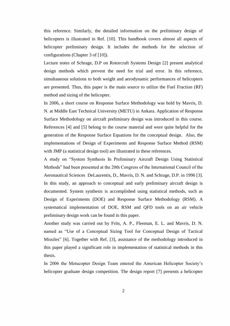
2.2 Selection of Helicopter Configuration

The feasible domain of helicopter configurations is defined by the requirements

which stem from both aerodynamic and weight analyses. A unique relation between

these analyses is the fuel weight ratio (RF). The Fuel Fraction (RF) Method utilizes

this relation to determine feasible helicopter configurations. An overall block

diagram of the RF sizing procedure is shown in Figure 2.1.

Figure 2.1 Configuration Selection and Evaluation Method

Initially, it is desired to investigate the variation of the disk loading, solidity and tip

speed as design variables. The choice of these variables stems from the fact that these

Specific Fuel

Consumption

Blade

Section

..... ..... ..... ..... .... .....

..... ..... ..... ..... ..... .....

..... ..... ..... ..... ..... .....

Fuel to Gross

Weight Ratio

Power

Required

Solidity Tip

Speed

Disk

Loading

Wg

..... ..... ..... ..... .... .....

..... ..... ..... ..... ..... .....

..... ..... ..... ..... ..... .....

Fuel to Gross

Weight Ratio

Power

Required

Solidity Tip

Speed

Disk

Loading

Wgo

p

RF Method:

Optimize gross weight

for a given configuration

Variables: Disk loading,

Tip Speed and Solidity

Number of

blades

Mission

Profile

Useful Load

Unfiltered

Selection

of Viable

Design

Points

Filtered

OEC CALCULATION

7

are considered as the most critical design parameters defining the characteristics of

the main rotor [1].

The design variables such as airfoil type and number of blades are external inputs or

can be selected before by just considering the competitors and have less importance

in the conceptual sizing process.

The program (RF code) determines the point, where the required and available fuel

to gross weight ratios are equal. Then, that point becomes a design point candidate.

In order the point to qualify as a design point, it is checked against various design

constraints. For instance, the design is checked against available thrust in hover, rotor

RPM limits, upper radius limit, etc. When a point qualifies as a design point, an

overall evaluation score is calculated at that design point to evaluate that specific

configuration in terms of the customer requirements.

2.2.1 Fuel Fraction (RF) Method Based Sizing and Overall Evaluation

Criteria

Generally, the design requirements include range and endurance performance

parameters of the helicopter. By implementation of parametric analysis a minimum

required RF can be defined as a function of selected major design variables. On the

other hand, the maximum available RF can also be evaluated with the same

parameters. The feasible helicopter configuration is the one with minimum required

RF is no less than the maximum RF available.

After the determination of all feasible configurations in design space, further

analyses is conducted to decide which configuration is the optimum in terms of the

selected Overall Evaluation Criteria and some other constraints.

2.2.1.1 Fuel Fraction (RF) Analysis for Hover Performance

In some applications, the RF analysis is applied for only disk loading variation. An example RF

analysis is given in

8

Figure 2.2. In this figure both locus of minimum gross weight and the feasible design

area for disk loading w1 (shaded area) are presented.

Figure 2.2 RF Method [10]

Intersection of RFr and, RFav for each disk loading defines a minimum gross weight

for that configuration. If the objective of the design is to select the minimum gross

weight configuration, the optimum configuration could be determined with this

analysis only.

The RF (Fuel Fraction) Method employed in this study is an extended version which

investigates the effect of different main rotor configuration variables on helicopter

design gross weight. These variables are disk loading, solidity and tip speed.

The following equations ((2.1) and (2.2)) are the main equations which are employed

to estimate the minimum design gross weights for different configurations [10]:

G

HRRF

W

THPCR ,

(2.1)

9

Where, RF,R is required fuel to gross weight ratio, C is specific fuel consumption in

lb/hp/lb, HPR is required power in hover horse power, hp, TH is required thrust at

hover and WG is gross weight.

G

empty

G

useful

AVFW

W

W

WR 1,

(2.2)

Where, RF,AV is available fuel to gross weight ratio, Wuseful is useful load including

only payload and crew, Wempty is the empty weight and WG is gross weight of the

aircraft.

In RF equations (2.1) and (2.2), the weight terms Wuseful, Wempty and WG are all

interrelated and Wuseful is a known parameter from the design requirements. The

power parameters, hp and TH are determined with the utilization of Blade Element

Moment Theory [1] in the RF code. During the analysis, the specific fuel

consumption (C) is assumed to be the average of the competitor helicopters‟ specific

fuel consumptions.

After a number of iterations, the gross weight, at which the required fuel to gross

weight ratio is equal to available fuel to gross weight ratio (minimum gross weight

point), is found as a feasible design point. For some points iterations may not

converge. This occurs when there is no feasible design point in that specific range of

gross weight for that configuration of design variables.

2.2.1.2 Overall Evaluation Criterion (OEC)

The need for an overall evaluation method arises when there is more than one

objective that a product or process is expected to satisfy. Situations of this nature are

common in many areas of aerospace applications.

In this thesis, since the main goal is to meet the customer requirements, utilization of

a multi objective method (OEC) which is based on the most significant requirements

becomes necessary.

10

ref ref ref refA B C DOEC

A B C D (2.3)

Equation (2.3) illustrates the structure of an OEC. In this equation, the Greek

symbols α, β, θ and φ stand for the weight of significant design parameters (A, B, C

and D) which are non-dimensionalized with their reference values. Significant

parameters and weight of them are determined through QFD analysis. Reference

values, on the other hand, are selected to be the value of that parameter for a

competitor helicopter.

2.2.1.3 RF Analysis for Forward Flight

Forward flight performance is yet another flight condition to be analyzed. The

dynamics of forward flight are quite different from the dynamics of hover. Thus, in

order to improve conceptual sizing and to account for the forward flight

performance, a new RF code is developed to see if the forward flight performance

requirements are satisfied.

Method employed for the forward flight RF analysis is the same as RF analysis for

hover. That is, when required fuel to gross weight ratio is equal to available fuel to

gross weight ratio the corresponding gross weight becomes the minimum gross

weight point for that configuration of variables. The derivation of the equations that

are used in the code can be found in [2].

For this analysis, the performance of the selected (for the hover performance)

configuration is inspected for the forward flight covering the whole mission profile.

3/ 2

1/ 21 1 1 11 1.05

1 1 1 1

UG

R T

R R G

U

WW

A K A K w

A K A K W

W

(2.4)

11

In equation (2.4), AR and AT are range and hover parameters, respectively [2]. The

range parameter AR depends on mission range, specific fuel consumption, cruise

velocity and lift to drag ratio at that velocity. AT, on the other hand, depends on

hover time, hover efficiency, disk loading and Figure of Merit. K represents the

weight correction factor and for this analysis it is taken to be 0.06 (value for self

sealing tanks) [2]. WG and WU are gross and useful loads in lb. Φ stands for the

empty to gross weight ratio and given as an initial guess which is close to the

competitors values. Since the gross weight appears at both sides of the equation, the

solution is iterative.

2.3 Parameter Sensitivity Analysis

Parameter sensitivity analysis is a method to determine system sensitivity to changes

in design variables values. This information can be used to decide which parameters

should be optimized or determined more accurately through further design studies.

Design of

Experiments

Response

Surface

Analysis

Design

Variables &

Ranges

RF analysis for

Experiment

Points

Monte Carlo

Analysis

Sensitivity of

Design

Sensitivity of

Design

Figure 2.3 Sensitivity Analysis Method

12

In this thesis, a statistical parameter sensitivity analysis methodology is employed to

determine the sensitivity of the design to possible changes of design variables. The

flowchart of the method adopted is given in Figure 2.3).

First, with the utilization of Design of Experiment entire design space is explored in

a more time effective manner when compared to traditional (Full Factorial) methods.

After the experiment points are determined, the RF code is employed for all these

design points and the responses (Gross Weight, Horse Power and OEC) are

collected. Next, the design points and the corresponding response values are inserted

to JMP program for the generation of Response Surface Equations for each response.

Finally, these equations are fed into Monte Carlo Analysis to find out how the design

is sensitive to the changes in design variables.

2.3.1 Design of Experiment (DOE)

With the ever-increasing complex and numerically time consuming models, design

of experiment has become an essential part of the modeling process. One way to run

tests is to test every possible combination of variables. In that case, the problem

grows very rapidly, especially for aerospace applications since they are

multidisciplinary problems. When the number of variables is high, it becomes very

cumbersome to compute all the possible combinations of the variables at three levels.

Consequently, a full factorial analysis becomes impractical. For instance, a problem

with six variables all having three levels, a full factorial design needs 35 = 243 runs.

On the other hand, with the use of DOE methods such as Box-Behnken (BB) design

or Central Composite Design (CCD), one would need 46 or 2n +2n+1 = 43 runs,

respectively.

In this thesis, for the DOE, BB method is selected to be employed for some of its

advantages which will be explained in the following section.

13

2.3.1.1 Box-Behnken (BB) Designs

BB designs are rotatable and for a small number of factors (four or less), they require

small number of runs. By avoiding the corners of the design space, they allow

designers to work around extreme factor combinations. As it can be seen in the BB

geometry shown in Figure 2.4, the axes show the variation of design variables (for

this case, 3 variables) while the points on the cube illustrate the experiment points.

Figure 2.4 BB Design Points

2.3.2 Response Surface (RS) Analysis

Most engineering design problems require experiments and/or simulations to

evaluate design objective and constraints as functions of design variables. For

example, in order to find the optimal airfoil shape for an aircraft wing, an engineer

simulates the air flow around the wing for different shape parameters (length,

curvature, material, etc.). On the other hand, a single simulation run can take many

minutes, hours, or even days to complete. As a result, routine tasks such as design

optimization or sensitivity analysis become impossible since they require thousands

or even millions of simulation evaluations. One way of alleviating this burden is to

construct approximation models, known as surrogate models (Response Surface

14

Equations) that mimic the behavior of the simulation model as closely as possible

while being computationally cheap to evaluate. Surrogate models are constructed

employing a data-driven, bottom-up approach. The exact, inner working of the

simulation code is not assumed to be known (or even understood), only the input-

output behavior is important. A model is constructed based on modeling the response

of the simulator to a limited number of intelligently chosen data points by the use of

the DOE. This approach is also known as behavioral modeling or black-box

modeling [4].

The accuracy of the surrogate models depends on the number and location of

samples in the design space. Various designs of experiments (DOE) techniques cater

to different sources of errors, in particular errors due to noise in the data or errors due

to an improper surrogate model [5]. The most popular surrogate models are

polynomial response surfaces. For most problems, the nature of true function is not

known a priori; thus it is not clear which surrogate model will be most accurate. In

addition, there is no consensus on how to obtain the most reliable estimates of the

accuracy of a given surrogate.

The simplest such model has the quadratic form containing linear terms for all

factors, squared terms for all factors, and products of all pairs of factors. Designs for

fitting these types of models are known as response surface designs.

2

0

1 1

k k k

i i ii i ij i j

i i i j

R b b x b x b x x (2.5)

An example formulation of a second order Response Surface Equation (RSE) is

given in Equation (2.5) [6]. In this equation, bi‟s are regression coefficients for the

first degree terms, and xi, xj‟s are the design variables. bii‟s are coefficients for the

pure quadratic terms, bij‟s are coefficients for the cross-product terms (second order

interactions), and b0 is the intercept term. The xi terms are the main effects, the xi2

terms are the quadratic effects, and the xixj are the second order interaction terms. In

this study a statistical analysis program, JMP, is employed to ease calculations.

15

Figure 2.5 Pareto Plot [4]

Figure 2.5 represents an example of Pareto Plot. In this plot, the green bars show the

individual effect of parameters on the response. Scaled estimate column, on the other

hand, shows the relative magnitude and direction (sign) of corresponding term

(parameter). In the generation of Pareto plots, the effects of all parameters on a

response are evaluated separately using statistical methods and the data provided in

the DOE chart. This is held automatically by JMP program. Pareto plots provide an

insight about the sensitivity of a response to selected variables. These plots are also

employed to determine if a parameter has a contribution in variation of a response.

This property enables designer eliminate some insignificant variables.

In Figure 2.6, properties of an “actual by predicted” plot is given. In this plot, Data

(experiment) points from DOE, perfect fit for that case, mean of response and 95%

confidence lines are included. The DOE data points should be scattered evenly along

and very close to the Perfect Fit line if the assumed form of the analysis is correct. If

there is clumping or patterns, or the data is not close to the Perfect Fit line, the order

of the fit model may be inadequate (transformations or HOT (Higher Order Terms)

may be needed) or some variables may be set at their extreme values (upper or lower

bound) dominating the behavior.

16

Figure 2.6 Actual by Predicted Plot [5]

Below, an example prediction profiler is given as Figure 2.7 illustrating the

interactions of design variables with selected system responses. On this chart, one

can see the ranges of design variables and system response values at a fixed variable-

set setting (in the example, setting of variables are weight=450, Diameter=10, Nose

Length=22). These setting of variables can be altered by just dragging the dashed red

lines in right-left direction and the results can be seen instantaneously.

Figure 2.7 Prediction Profiler [6]

17

At the end of this analysis, if the fits for selected responses are accurate enough, the

equations of these fits (RSEs) can be employed instead of simulation runs, so that,

the time spent is decreased.

2.3.3 Monte Carlo Simulations

Monte Carlo Simulations are computer-based method of analysis developed in the

1940's. This method uses statistical sampling techniques in obtaining a probabilistic

approximation to the solution of a mathematical equation or model. They are widely

used for sensitivity analysis.

Generally, Monte Carlo simulations are characterized by a large number of unknown

parameters, many of which are difficult to obtain experimentally. Implementation of

this method is mainly accomplished by giving a random distribution [11] (gaussian

for our case) to design variables (main rotor radius, chord etc.) and looking after the

response/system behavior for these cases.

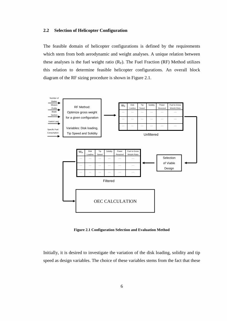
2.4 Conseptual Sizing of Main Components of Helicopter

2.4.1 Component Weights

The individual weights of main components can be estimated using emprical

formulations [2]. The equations are given below.

Main Rotor

0.342 1.58 0.631.7R GW W R (2.6)

Tail Rotor

18

0.446

1.62 0.667.121000

2 ; 0.2

GTR TR TR

TR TR

WW R

where and R R

(2.7)

Power Plant Section Group

1.07

0.542.5* *1000

GPS

WW dl (2.8)

Flight Control Group

0.712 0.6530.0226

.

FC G c

c

W W V

whereV is cruise speed inknots (2.9)

Landing Gear

0.975

0.04751000

GLG

WW (2.10)

Fuselage

0.598 0.9420.37F GW W R (2.11)

Using above equations, a first estimation for conceptual sizing of the main

components is done (section 3.5).

19

2.4.2 Dimension Characteristics

Similar to the weight estimations, there are some empirical equations presented in the

literature to make a first estimation of general dimensions of a helicopter in

conceptual design phase. Some of those equations [2] were given below.

Fuselage

1.6FL R (2.12)

Tail to Main Body

2 1.23T ML R (2.13)

Tail Rotor Radius

0.36TRR R (2.14)

Clearance

0.05ClL R (2.15)

Total Length

1.91TotalL R (2.16)

20

CHAPTER 3

3 CONCEPTUAL SIZING AND ANALYSIS

In this thesis, the multidisciplinary and probabilistic design approach is utilized. This

section provides an overview of this design procedure.

Design

Requirements

RF Method &

OEC Calculation

(for Hover)

Competitor

Study

Selection of most

important design variables

QFD Analysis

Voice of Engineer

DOE and

Response Surface

Analysis

RSE

Sensitivity

Analysis by Monte

Carlo Simulations

Selection of Best

Configuration

Evaluation of

Selected

Configuration

(for Forward Flight

Performance)

Effect of Change

in Selected

Variables

Configuration

of the

Helicopter

Figure 3.1 Flowchart of the Design Method

21

In Figure 3.1, steps of the conceptual sizing and analysis are illustrated. The design

requirements are treated as the “voice of the customer” and translated to the “voice

of the engineer” through a Quality Functional Deployment (QFD) Matrix (House of

Quality). The QFD matrix provides a market awareness of the proposed product as

well as showing the most dominant design parameters. The weighted sums are then

used to establish an “Overall Evaluation Criteria” (OEC) to rank different helicopter

configurations.

Since the main rotor is known to be the heart of a helicopter design and a major

contributor to almost every aspect of the helicopter, the design space is swept for

disk loading, tip speed and solidity, and their design viability is checked. These three

parameters are known to be the core design parameters in main rotor design [1]. For

each main rotor configuration an in-house developed helicopter design algorithm is

employed. This algorithm sizes the helicopter and calculates parameters like gross

weight, radius, power required, range, endurance, etc. [2]. Also the OEC for all the

points in design space are evaluated in this code. The higher the OEC, the better the

performance of the helicopter, in terms of customer needs, where OEC parameter

weight values are determined based on the outcome of the QFD solution. On the

other hand, there are some other constraints to be considered in helicopter design

such as structural issues. As a result, in the light of OEC results and constraints, the

best configuration is selected for the hover performance.

Then, the relationship of disk loading, tip speed, solidity and some other design

variables to the target design drivers, such as gross weight, are fit into a DOE

scheme. Next, Response Surface Equations are generated. Then, using these

equations, Monte Carlo Simulations are performed to evaluate the sensitivities of the

design variables to the target values. Finally, the performance of the selected

configuration is checked for forward flight.

After the final configuration of the desired helicopter is attained, the conceptual

sizing of some main components is performed utilizing some empirical formulas.

22

3.1 Design Requirements

Considering the necessities and the geographical conditions of Turkey, the following

sample requirements are selected for this study:

Service Ceiling: 15.000ft

HIGE: 10.000ft

Operational Temp: ISA+35

Endurance: 180 min.

Range: 600km

Payload: 1pilot + 5 passengers + 200kg

Improved Safety

Multi-function capability

Low vibration

Fast forward speed

Rugged design

A helicopter with the above-mentioned specifications can be employed for multi-

purposes such as rescue, air ambulance and commercial transportation etc. missions.

Figure 3.2 shows a sample mission profile for the helicopter considered.

Figure 3.2 Reference Mission Profile

23

The details of the mission profile are given in Table 3.1.

Table 3.1 Mission Profile Segments

Segment Description Altitude (ft) Speed Time (min)

0 – 1 Warm-up 0 - 2

1 – 2 Takeoff. Vertical

Climb 0 – 5

- 2

2 – 3 Acceleration Ground

Effect 5

0 - 50 knots 1

3 – 4 Climb 5 – 6000 10 ft/s (R/C) 10

4 – 5 Cruise 6000 100 knots 15

5 Hover 6000 - 5

5 – 6 Descend 6000 – 0 10 ft/s (R/C) 10

6 – 7 Landing 0 - 5

3.2 Competitor Study

In this section, a competitor study is performed. This study is an initial step for most

of the engineering conceptual design work. Searching for similar helicopters, in

terms of mission and performance requirements, Eurocopter AS350 B3 and EC 120

are selected to be the two competitors. Some of the specifications [9] of these

helicopters are given in the Table 3.2. Reference values of some unknown

parameters are adapted from these helicopters‟ data to be employed as initial value in

the analyses.

24

Table 3.2 Competitor Helicopters’ Specifications

Competitor Eurocopter AS350 B3 Eurocopter EC 120

General Characteristics

Crew 1 Pilot 1 or 2 Pilots

Capacity 6 passengers 4 passengers

Length 10.93 m (35 ft 10.5 in) 9.6 m (31 ft 5 in)

Rotor diameter 10.69 m (35 ft 1 in) 10 m (32 ft 8 in)

Height 3.14 m (10 ft 3.5 in) 3.4 m (11 ft 2 in)

Empty weight 1174 kg (2588 lb) 991 kg (2185 lb)

Gross weight 2250 kg (4960 lb) 1715 kg (3781 lb)

Powerplant 1 Turbomeca Arriel 2B turboshaft,

632 kW (847 shp)

1 Turbomeca Arrius 2F

turboshaft, 376 kW (504 shp)

Performance

Never exceed speed 287 km/h (155 kts, 178 mph) 278 km/h, (150 kts, 172 mph)

Cruise speed 245 km/h (132 kts, 152 mph) 223 km/h, (120 kts, 138 mph)

Range 662 km (357 nmi, 411 mi) 710 km, (383 mi, 440 nm)

Service ceiling 4600 m (15100 ft) 5182 m (17000 ft)

Rate of climb 8.5 m/s (1675 ft/min) 5.84 m/s (1150 ft/min)

3.3 Quality Functional Deployment Analysis

A QFD Matrix, a concurrent engineering tool, is employed to translate the customer

requirements to engineering parameters. The engineering parameters are weighted

according to significance of their effects on the costumer requirements.

Figure 3.3 shows the QFD Matrix prepared for the requirements introduced in the

section 3.1.

25

Figure 3.3 QFD Matrix

Filling out the QFD matrix requires experience and a strong foundation in helicopter

theory [7]. The QFD matrix is created using the package program QFD Designer V4

(A.1).

First, the customer importance parameters are determined. In the determination of

this parameter customer requirements are considered in terms of their relative

importance. All the parameters under the “Customers Voice” heading are given a

26

weight between 1 and 5, from least important to the most important. For instance, the

weight of good autorotative capability is selected to be 5 since it is a crucial

parameter for the safety of helicopters. Then, the relation between customer

requirements and engineering parameters are determined1. For example, if the hover

efficiency row in the customer voice is inspected it is seen that this requirement has a

strong relationship with solidity, disk loading, figure of merit, maximum continuous

power, specific fuel consumption and power to weight ratio parameters. On the other

hand, it has a moderate relationship with tip speed, number of blades, empty weight,

number of engines and acquisition cost parameters. The relation of hover efficiency

with materials, hub type and level of autonomy performance is a weak one with

respect to other parameters. Finally, the empty spaces show that there are no direct

relationships between hover efficiency and short duration rating, RPM, Mean Time

Between Failure (MTBF), Mean Time To Repair (MTTR) and level of autonomy

safety parameters. After the QFD Matrix is filled out, the relative importance of the

engineering parameters appears at the QFD matrix in the weighted importance,

relative importance and rank rows.

As a result the QFD analysis yields following parameters as the most important

design drivers in significance order:

Disk Loading

Empty Weight

Figure of Merit

Hub Type

1 The weight of symbols in the QFD Matrix is as: = 1 (weak), = 3 (moderate) and = 9

(high).

27

Based on this analysis, a preliminary sizing is done and a first configuration is

selected as it will be explained in the following sections.

3.4 Selection of Helicopter Configuration

3.4.1 Helicopter Preliminary Sizing Using OEC and RF-Optimization

In accordance with the output of the QFD analysis performed in the previous section,

the following OEC is used to evaluate the performance of different configurations.

ref ref ref refGW hp dl RFOEC

GW hp dl RF (3.1)

where the letters α, β, θ and φ indicate the weights of the parameters, gross weight

(GW), required horse power (Hp), disc loading (DL) and Required Fuel Weight

Ratio in hover (RF), respectively. Each of these parameters is normalized with their

reference values (values for AS 350 2B see Table 3.2). The weight of each ratio is

obtained from the corresponding weights acquired through the QFD results. The RF

analysis for hover is employed.

As a result, a number of helicopter designs are obtained and ranked according to

OEC scores. In Figure 3.4, a 3-D plot of the design space indicates the performance

of different configurations, based on the OEC (evaluation) score.

28

Figure 3.4 OEC Variation

It is observed that as the tip speed, solidity, and disc loading decreases, the

configuration approaches to an optimum in terms of OEC. In Figure 3.4 the cube

presented by red lines designates the range for solidity, tip speed and disk loading in

this analysis. The empty parts inside the cube are due to the fact that no viable design

points were obtained at that region. In terms of the color codes, a better design (high

OEC) is obtained while going from blue to red regions.

On the other hand, helicopter design is limited by some other constraints. This is an

expected issue since physically; there should be a limitation on the desirable design.

For instance, for some points, the main rotor radius becomes too long and this leads

to structural problems. Another problem is that, an increase in blade radius causes a

decrease in the rigidity of the blade, therefore, a higher rotor RPM is required to keep

the blades rigid. However, with long blades and low tip speeds, the rotor RPM would

be relatively low, so rigidity cannot be maintained for such configurations.

Consequently, when the configurations are sorted for decreasing evaluation score

(first fifteen are given in Table 3.1). The tenth configuration is selected since it has a

considerably high evaluation score and rational physical properties. Note that,

choices with higher scores tend to have low chord numbers making the rotor design

difficult from a structural stand-point. Since the RF method has no structural models

29

such decisions are made off-line. Of course it would be possible to include a

structural model in the methodology.

Table 3.3 First Fifteen Configurations in terms of OEC Score

Rank Evaluation

Score

DL

(lb/ft2)

TS (ft/s) SLD GW (lb) Radius (ft) chord (ft) RPM hp

1 6.23 4 600 0.05 3450 16.57 0.65 345.78 278.7173

2 6.12 4 650 0.05 3475 16.63 0.65 373.24 288.9547

3 6.1 4 600 0.06 3500 16.69 0.79 343.29 290.2042

4 5.99 4.5 600 0.05 3425 15.56 0.61 368.22 283.6378

5 5.95 4 650 0.06 3550 16.81 0.79 369.24 306.1738

6 5.94 4 700 0.05 3525 16.75 0.66 399.07 309.2835

7 5.93 4 600 0.07 3575 16.86 0.93 339.83 307.0874

8 5.87 4.5 600 0.06 3475 15.68 0.74 365.40 295.5514

9 5.86 4.5 650 0.05 3450 15.62 0.61 397.37 298.3276

10 5.83 4 600 0.08 3625 16.98 1.07 337.43 316.9268

11 5.79 4 750 0.05 3575 16.87 0.66 424.53 327.4265

12 5.78 4 650 0.07 3625 16.98 0.93 365.55 324.8547

13 5.77 4 700 0.06 3600 16.93 0.8 394.83 328.3605

14 5.75 4.5 650 0.06 3500 15.73 0.74 394.59 308.8868

15 5.74 4.5 600 0.07 3525 15.79 0.87 362.86 309.1467

Up to this point of the study, the RF analysis was utilized for all of the possible

design configurations. The RF code was run for every case and the results were

collected. This was a full factorial experiment and was time consuming. In the

following part, to be able to make the sensitivity analysis in a time efficient manner,

Design of Experiment (DOE) and Response Surface methods will be employed.

3.4.2 DOE & Response Surface (RS) Analysis

In this section, first the design variables are determined. The selection of variables

may affect the accuracy of the Response Surface fits. In order to account for this

30

issue, two different set of variables are generated and employed. First set of (CASE1)

design parameters are blade twist, tip speed, disk loading and solidity. Second set

(CASE2) includes blade twist, main rotor radius, RPM, chord parameters. CASE1

parameters are a combination of rotor geometric parameters and generally give better

physical inside to the design. CASE2 variables are the base variables for a helicopter

main rotor.

After the experiments are designed, a response surface analysis is conducted. In this

analysis, gross weight, horse power and evaluation score are selected to be the

responses.

In the beginning, for both cases, a first order estimation is carried out to see if it

would be accurate enough and to make an initial sensitivity analysis. Purpose of this

rough sensitivity analysis is to retrieve some clue about the effects of the selected

design variables on the responses. Much better information about the sensitivity will

be gathered from the Monte Carlo analysis.

Since the fits for first order estimation are not accurate enough to be employed in

Monte Carlo simulations, second order estimations are done in order to improve the

accuracy of fits (response surface equations).

3.4.2.1 Analysis with CASE1 Parameters

In this analysis, the variables which are listed in the Table 3.4 below are inserted and

27 experiments are generated with DOE tool of JMP program. The second column of

Table 3.4 illustrates the pattern of the design variables for each experiment points. It

should be noted that for five of the experiments the pattern index is found as “0”. At

these points all the design variables have their average values. The reason behind

repeating the same experiment at this point for five times is just to check the

reliability of the supplied data. This is an embedded property of JMP program and

whenever a DOE is generated these check points are included in the experiments

automatically.

After the DOE is ready, hover RF code is run for these experiment points.

31

Next, the outputs of the RF code are implemented to the JMP data table as the actual

responses. At some experiment points (experiments 17 and 24 for this analysis) there

is no rational solution from the RF code. Consequently, these points were excluded

from the analysis.

Table 3.4 CASE1 BB Design Variables

Design Variables (Factors) Responses

Experiment

Number Pattern2 Twist (°) TS DL Solidity Gweight HP

Evaluation

Score

1 −0+0 -8 750 8 0.07 3580 404.317 4.47

2 −00− -8 750 6 0.05 3490 347.7 5.1

3 0 -6 750 6 0.07 3630 390.603 4.81

4 0+−0 -6 900 4 0.07 4640 730.168 4.18

5 0 -6 750 6 0.07 3630 390.603 4.81

6 −−00 -8 600 6 0.07 3480 331.562 5.21

7 0+0− -6 900 6 0.05 3640 407.358 4.73

8 +00− -4 750 6 0.05 3510 356.24 5.04

9 0 -6 750 6 0.07 3630 390.603 4.81

10 00−+ -6 750 4 0.09 4060 466.921 4.93

11 +00+ -4 750 6 0.09 3770 434.367 4.56

12 00++ -6 750 8 0.09 3690 440.23 4.27

13 +0−0 -4 750 4 0.07 4030 491.838 4.86

14 0−0+ -6 600 6 0.09 3580 359.366 4.99

15 0 -6 750 6 0.07 3630 390.603 4.81

16 0−−0 -6 600 4 0.07 3570 309.542 5.91

173 0−0− -6 600 6 0.05 10010 819.227 -9

2 “0“ means average value of the variable, “+” means maximum value of the

variable, “-“ means minimum value of the variable.

3 The RF code finds no solution at this point.

32

Table 3.4 Continued

Design Variables (Factors) Responses

Experiment

Number Pattern Twist (°) TS DL Solidity Gweight HP

Evaluation

Score

18 0+0+ -6 900 6 0.09 4060 548.618 4.1

19 0++0 -6 900 8 0.07 3740 472.413 4.14

20 −00+ -8 750 6 0.09 3750 423.358 4.61

21 −+00 -8 900 6 0.07 3830 473.198 4.4

22 00−− -6 750 4 0.05 3580 330.68 5.76

23 −0−0 -8 750 4 0.07 3780 383.291 5.38

244 0−+0 -6 600 8 0.07 10010 892.977 -9

25 +−00 -4 600 6 0.07 3500 339.572 5.14

26 00+− -6 750 8 0.05 3520 386.341 4.58

27 0 -6 750 6 0.07 3630 390.603 4.81

Then using JMP, a first order response surface analysis is performed. Results of this

analysis can be summarized as follows.

TS(600,900)

DL(4,8)

Solidity(0,05,0,09)

tw ist(-8,-4)

Term

150,5956

-124,2313

104,7996

32,3316

Orthog

Estimate

Pareto Plot of Transformed Estimates

Figure 3.5 Pareto Plot for Gweight Response for CASE1

4 The RF code finds no solution at this point.

33

Figure 3.5 shows the effect of each variable on the gross weight. According to this

analysis, tip speed seems to be the most significant parameter in gross weight

estimation. Disk loading and solidity also seem to have comparable effects on gross

weight. Twist, on the other hand, has the lowest effect on this response.

TS(600,900)

Solidity(0,05,0,09)

DL(4,8)

tw ist(-8,-4)

Term

64,62573

32,56990

-17,07320

14,06166

Orthog

Estimate

Pareto Plot of Transformed Estimates

Figure 3.6 Pareto Plot for Horse Power Response for CASE1

Similar to the gross weight response, again tip speed appears to be the most and twist

appears to be the least effective parameter for horse power response with a higher

percentage (Figure 3.6). Only difference is that the ranks of DL and solidity are

changed.

TS(600,900)

DL(4,8)

Solidity(0,05,0,09)

tw ist(-8,-4)

Term

-0,3309023

-0,2314476

-0,1843044

-0,0640859

Orthog

Estimate

Pareto Plot of Transformed Estimates

Figure 3.7 Pareto Plot for Evaluation Score Response for CASE1

This time, for the evaluation score response, in Figure 3.7, again the tip speed is the

dominating factor. Actually, the order of variables is the same with the horse power

response, but the relative effect of the variables is different for the two responses.

From the three Pareto plots above, it can be concluded that, twist has a negligible

effect on all of responses. Thus, if the number of variables and experiments were

34

large, the blade twist parameter could be excluded for the following parts of the

analysis. Contrarily, since the number of experiments is small enough to be handled,

the twist is maintained as a design variable in order to be able to make more reliable

comparisons.

RSquare

RSquare Adj

Root Mean Square Error

Mean of Response

Observations (or Sum Wgts)

0,752774

0,703329

143,4714

3734

25

Summary of Fit

RSquare

RSquare Adj

Root Mean Square Error

Mean of Response

Observations (or Sum Wgts)

0,71147

0,653764

53,87868

423,7541

25

Summary of Fit

RSquare

RSquare Adj

Root Mean Square Error

Mean of Response

Observations (or Sum Wgts)

0,885734

0,86288

0,180099

4,77

25

Summary of Fit

a)GW b) HP c) OEC

Figure 3.8 Summary of Fits for CASE1

Above charts are taken for the first order fits of three responses (Figure 3.8). As it

can be expected, first order fit is not adequate for all of our responses (RSquare terms

are much less then 1). On the other hand this is a very useful analysis to have a first

idea about the sensitivity of the responses to given factors. After this point, for a finer

estimate, a second order response surface analysis is performed for the same data

given in Table 3.1.

3400

3600

3800

4000

4200

4400

4600

4800

Gw

eig

ht A

ctu

al

3250 3500 3750 4000 4250 4500 4750

Gw eight Predicted P<.0001

RSq=0,97 RMSE=75,081

Figure 3.9 CASE1 2nd Order Fit for Gross Weight Response

35

Figure 3.9 reveals that, for a second order estimation, gross weight response can be

fitted with an adequate accuracy (RSquare = 0.97).

300

350

400

450

500

550

600

650

700

750

Hp A

ctu

al

300 400 500 600 700

Hp Predicted P<.0001

RSq=0,95 RMSE=31,04

Figure 3.10 CASE1 2nd

Order Fit For Horse power

Similar to gross weight response, also the accuracy of second order fit seems to be

sufficient for horse power response (Figure 3.10).

4

4,5

5

5,5

6

Eval A

ctu

al

4,0 4,5 5,0 5,5 6,0

Eval Predicted P<.0001

RSq=0,98 RMSE=0,0972

Figure 3.11 CASE1 2nd

Order Fit for Evaluation Score

36

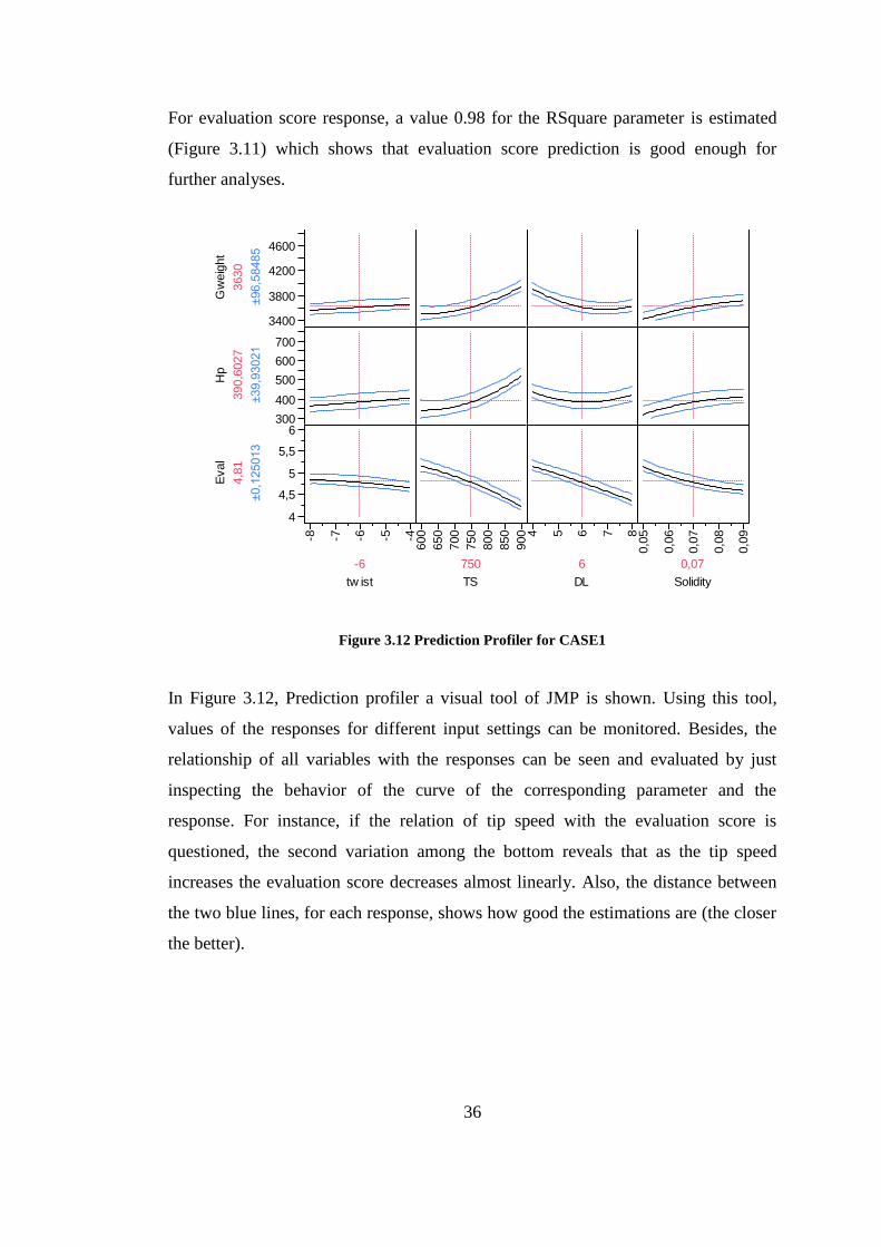
For evaluation score response, a value 0.98 for the RSquare parameter is estimated

(Figure 3.11) which shows that evaluation score prediction is good enough for

further analyses.

3400

3800

4200

4600

Gw

eig

ht

3630

±96,58485

300

400

500

600

700

Hp

390,6

027

±39,93021

4

4,5

5

5,5

6

Eval

4,8

1

±0,125013

-8 -7 -6 -5 -4

-6

tw ist

600

650

700

750

800

850

900

750

TS

4 5 6 7 8

6

DL

0,0

5

0,0

6

0,0

7

0,0

8

0,0

9

0,07

Solidity

Prediction Profiler

Figure 3.12 Prediction Profiler for CASE1

In Figure 3.12, Prediction profiler a visual tool of JMP is shown. Using this tool,

values of the responses for different input settings can be monitored. Besides, the

relationship of all variables with the responses can be seen and evaluated by just

inspecting the behavior of the curve of the corresponding parameter and the

response. For instance, if the relation of tip speed with the evaluation score is

questioned, the second variation among the bottom reveals that as the tip speed

increases the evaluation score decreases almost linearly. Also, the distance between

the two blue lines, for each response, shows how good the estimations are (the closer

the better).

37

3.4.2.2 Analysis with CASE2 Parameters

In this part, CASE2 variables are chosen to be DOE factors and the analysis is

performed for the same responses. In Table 3.5, design variables Rad and Chord

stand for main rotor radius and root chord respectively. There is a no solution point

(Experiment number 7) for this case either, and it is excluded from the analysis.

Table 3.5 CASE2 BB Design Variables

Design Variables (Factors) Responses

Experiment

Number Pattern Rad Chord RPM

Twist

(°) Gweight HP

Evaluation

Score

1 +0−0 20 0.9 300 -6 3640 292.648 6.7

2 −00− 15 0.9 400 -8 3560 334.45 5.38

3 0 17.5 0.9 400 -6 3730 364.212 5.55

4 110+0− 17.5 1.2 400 -8 3930 423.191 5.1

5 +00− 20 0.9 400 -8 4000 439.547 5.51

6 00−− 17.5 0.9 300 -8 3510 276.905 6.39

75 −0−0 15 0.9 300 -6 10010 268.733 -9

8 +00+ 20 0.9 400 -4 4550 701.243 4.44

9 0−+0 17.5 0.6 500 -6 3750 402.122 5.35

10 0+0+ 17.5 1.2 400 -4 4170 541.501 4.54

11 0++0 17.5 1.2 500 -6 4720 785.062 3.76

12 +−00 20 0.6 400 -6 3710 350.196 6.22

13 −+00 15 1.2 400 -6 3690 372.877 5.05

5 The RF code finds no solution at this point.

38

Table 3.5 Continued

Design Variables (Factors) Responses

Experiment

Number Pattern Rad Chord RPM

Twist

(°) Gweight HP

Evaluation

Score

14 00+− 17.5 0.9 500 -8 4060 509.961 4.71

15 0+−0 17.5 1.2 300 -6 3640 308.983 5.99

16 0 17.5 0.9 400 -6 3730 364.212 5.55

17 0−0− 17.5 0.6 400 -8 3530 305.124 6.13

18 0 20 1.2 400 -6 4640 692.671 4.39

19 −0+0 15 0.9 500 -6 3760 418.688 4.78

20 −−00 15 0.6 400 -6 3430 299.773 5.74

21 −00+ 15 0.9 400 -4 3570 341.174 5.33

22 00++ 17.5 0.9 500 -4 4670 802.34 3.77

23 0 17.5 0.9 400 -6 3730 364.212 5.55

24 0−0+ 17.5 0.6 400 -4 3540 310.937 6.08

25 0−−0 17.5 0.6 300 -6 3390 250.83 6.79

26 00−+ 17.5 0.9 300 -4 3520 282.34 6.33

27 17.5 0.9 400 -6 3730 364.212 5.55 17.5

Similar to CASE1, Pareto plots are taken from first order fit to be able to see direct

effects of the CASE2 variables on each response.

RPM(300,500)

Rad(15,20)

Chord(0,6,1,2)

tw ist(-8,-4)

Term

298,00736

231,49450

194,75165

80,95781

Orthog

Estimate

Pareto Plot of Transformed Estimates

Figure 3.13 Pareto Plot for Gweight Response for CASE2

39

Figure 3.13 shows the effect of each CASE2 variable on the gross weight. Among the

four factors, RPM is the most significant and the twist is the least. Since the product

of RPM and the radius gives the tip speed, this is an expected result if we look at the

same analysis for CASE1 variables.

RPM(300,500)

Rad(15,20)

Chord(0,6,1,2)

tw ist(-8,-4)

Term

131,61118

76,54943

68,23691

39,08384

Orthog

Estimate

Pareto Plot of Transformed Estimates

Figure 3.14 Pareto Plot for Horse Power Response for CASE2

For the horse power response, again the RPM comes out to be the most effective

parameter (Figure 3.14) and its relative effect is higher when compared to its effect

in gross weight response.

RPM(300,500)

Chord(0,6,1,2)

tw ist(-8,-4)

Rad(15,20)

Term

-0,6893209

-0,4234716

-0,1545558

-0,0419201

Orthog

Estimate

Pareto Plot of Transformed Estimates

Figure 3.15 Pareto Plot for Evaluation Score Response for CASE2

Figure 3.15 illustrates the effect of parameters to evaluation score. RPM is again the

most effective one here, but the order of other variables is altered. Also, this is the

first time at which twist is not the least effective parameter for a response. Effect of

40

the main rotor radius on evaluation score response seems to be negligible when

compared to other design parameters.

RSquare

RSquare Adj

Root Mean Square Error

Mean of Response

Observations (or Sum Wgts)

0,828907

0,796318

218,5354

3901,923

26

Summary of Fit

RSquare

RSquare Adj

Root Mean Square Error

Mean of Response

Observations (or Sum Wgts)

0,782303

0,740837

100,5846

444,7264

26

Summary of Fit

RSquare

RSquare Adj

Root Mean Square Error

Mean of Response

Observations (or Sum Wgts)

0,895448

0,875534

0,31356

5,337692

26

Summary of Fit

a)GW b) HP c) OEC

Figure 3.16 Summary of Fits for CASE2

Although the Pareto plots of the first order estimation are useful and to be taken as a

check point for the sensitivity analysis, from the data given in Figure 3.16, it can be

concluded that the fits are not accurate enough. Therefore, a second order estimation

analysis is performed in order to have an improved accuracy.

3500

4000

4500

5000

5500

Gw

eig

ht A

ctu

al

3500 4000 4500 5000 5500

Gw eight Predicted P<.0001

RSq=0,99 RMSE=69,58

Figure 3.17 CASE2 2nd

Order Fit For Gross Weight

In Figure 3.17, variation of actual gross weight with respect to the predicted one for

CASE2 is illustrated. When compared to same figure for CASE1, the difference is

obvious. In this case prediction curve is very close to the experiment points. The

gross weight fit for this case has an RSquare value of 0.99 (very close to 1) and a

41

RMSE value of 69.58 for the gross weight response. This result unveils that, the

gross weight prediction with these (CASE2) variables is better than the prediction

obtained the CASE1 variables.

200

300

400

500

600

700

800

900

1000

1100

HP

Actu

al

200 300 400 500 600 700 800 900 1100

HP Predicted P<.0001

RSq=0,99 RMSE=32,765

Actual by Predicted Plot

Figure 3.18 CASE2 2nd

Order Fit For Horse Power

Similarly, fit for the horse power response is better than the one for the CASE1 fit

(Figure 3.18). While the RSquare value is 0.95 for the CASE1, it is 0.99 for this case.

3,5

4

4,5

5

5,5

6

6,5

7

Eval A

ctu

al

3,5 4,0 4,5 5,0 5,5 6,0 6,5 7,0

Eval Predicted P<.0001

RSq=0,99 RMSE=0,112

Figure 3.19 CASE2 2nd

Order Fit For Evaluation Score

42

In the Figure 3.19, fit for the evaluation score is given. RSquare value for this case

comes out to be 0.99 which is closer to 1 when compared the CASE1 fit.

3500

4000

4500

5000

5500G

weig

ht

3621,8

3

±99,45451

200

400

600

800

1000

HP

315,6

326

±46,8329

3,5

4,5

5,5

6,5

Eval

5,8

31078

±0,160073

15

16

17

18

19

20

17

Rad

0,6

0,7

0,8

0,9 1

1,1

1,2

1,07

Chord

300

350

400

450

500

337

RPM

-8 -7 -6 -5 -4

-7,8

tw ist

Prediction Profiler

Figure 3.20 Prediction Profiler for CASE2

When Figure 3.20 and Figure 3.12 are inspected closely, it is obvious that, the fits are

much better for this case (the blue curves are closer to each other than they were in

CASE1).

Up to this point, first a full factorial analysis was performed for sizing based on the

hover performance (section 3.4). Next, with the use of RSM and DOE, an initial

sensitivity analysis (with Pareto plots) and RSE generation were performed for two

different cases. After this point, CASE2 design variables will be employed in further

analysis since it results in a more accurate fits for the selected responses.

RSE coefficients for the second order fit for CASE2 analysis, are given in

Table 3.6, where intercept term corresponds to b0 of Equation 2.4.

43

Table 3.6 RSE Coefficients

Term Gweight Hp Eval

Intercept 3730 364.21249 5.55

Rad(15.20) 339.41667 108.91243 -0.09825

Chord(0.6.1.2) 286.66667 100.44202 -0.623333

RPM(300.500) 400.25 175.33972 -0.999083

twist(-8.-4) 119.16667 57.529854 -0.2275

Rad*Chord 167.5 67.342819 -0.285

Rad*RPM 404.25 186.60813 -0.50525

Chord*RPM 180 81.196713 -0.1975

Rad*twist 135 63.743187 -0.255

Chord*twist 57.5 28.124428 -0.1275

RPM*twist 150 71.736046 -0.22

Rad*Rad 164.33333 76.342655 -0.230917

Chord*Chord -14.04167 -5.878535 0.0367083

RPM*RPM 178.08333 87.169238 -0.102167

twist*twist 44.708333 22.302413 -0.142042

In RSE, all the variables are taken with their non-dimensional values. These non-

dimensional terms are given as follows;

17.5 / 2.5

0.9 / 0.3

400 /100

6 / 2

nonDim

nonDim

nonDim

nonDim

R Rad

c c

RPM RPM

twist twist

Since the RSE is ready, Monte Carlo analysis can be held. Results of Monte Carlo

analysis are presented in the following section.

3.4.3 Monte Carlo Analysis

44

In section 3.4, an optimum configuration is selected for the hover performance

analysis. Since the conceptual sizing is an early phase of helicopter design, some

chosen parameters cannot be maintained during the considerably long period of

design effort. On the other hand, evaluation score should be kept around some

optimal point to ensure the satisfaction of design requirements.

Monte Carlo analysis is used to make a sensitivity analysis to find out the sensitivity

of the evaluation score to the CASE2 design variables for the configuration found

before (Table 3.3).

In this section, RSE generated in previous section is employed in the Monte Carlo

analysis.

First, each of the CASE2 variables is given a normal distribution (Figure 3.21 a, b, c,

d). Changing only one of the variables (10000 run for each variable) and keeping the

others constant, four evaluation score distributions are found. The 3σ values for these

variables were given in the table below.

Table 3.7 Monte Carlo Parameters

Radius (ft) Chord (ft) RPM Twist (deg)

Base Value 16.984 1.07 337 -7.8

3σ value 1.7 0.107 33.7 0.78

45

Figure 3.21.a Distribution of Radius

Figure 3.21.b Distribution of Chord

46

Figure 3.21.c Distribution of RPM

Figure 3.21.d Distribution of Twist

Evaluation scores, calculated by the implementation of the RSE, have a distribution

as follows.

47

0 1000 2000 3000 4000 5000 6000 7000 8000 9000 100005.4

5.5

5.6

5.7

5.8

5.9

6

6.1

6.2

Run Number

Evalu

aio

n S

core

OECradius

OECchord

OECrpm

OECtwist

Figure 3.22 Monte Carlo Results

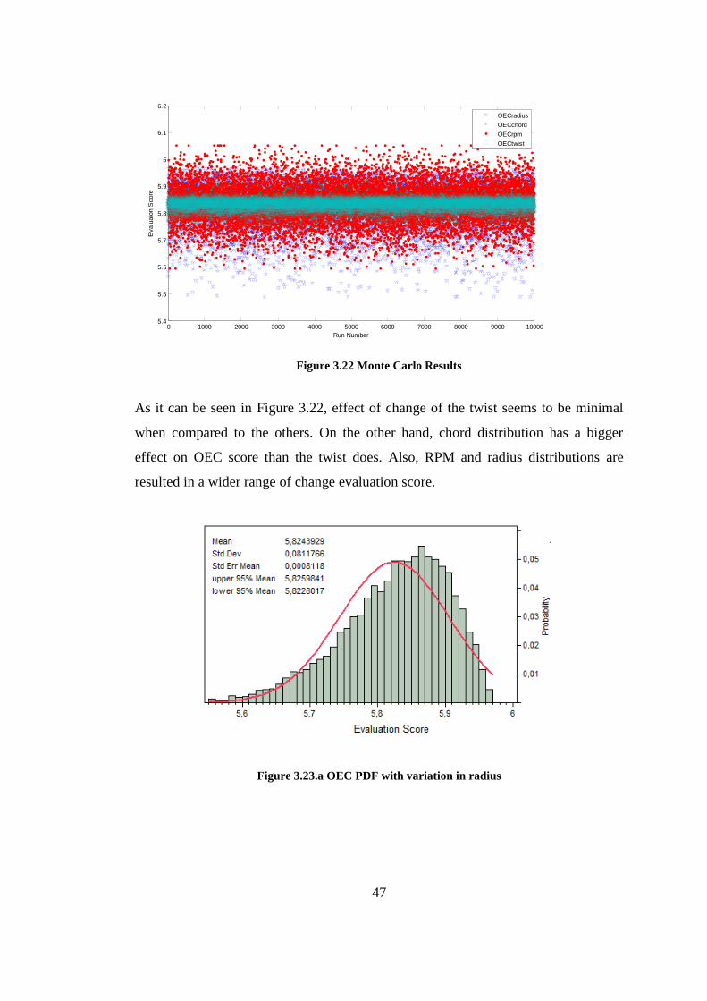
As it can be seen in Figure 3.22, effect of change of the twist seems to be minimal

when compared to the others. On the other hand, chord distribution has a bigger

effect on OEC score than the twist does. Also, RPM and radius distributions are

resulted in a wider range of change evaluation score.

Figure 3.23.a OEC PDF with variation in radius

48

Figure 3.23.b OEC PDF with variation in Chord

Figure 3.23.c OEC PDF with variation in RPM

49

Figure 3.23.d OEC PDF with variation in Twist

Monte Carlo results are illustrated as probability density distributions. All these

distributions resembles to a normal distribution since skewness values are about zero

(Figure 3.23 (a,b,c,d)).

Consequently, in terms of the sensitivity of the evaluation score to the change in

parameters, the design variables can be ordered as; RPM, radius, chord and twist

from the most to the least effective.

To be able to monitor the effect of all variables together, another Monte Carlo

analysis is carried out. In this analysis, all of the variables have their Monte Carlo

distribution (Figure 3.21 a, b, c, d).

50

0 1000 2000 3000 4000 5000 6000 7000 8000 9000 10000

5.4

5.5

5.6

5.7

5.8

5.9

6

6.1

6.2

6.3

Run Number

Evalu

ation S

core

Figure 3.24 MC results when all variables changed

Figure 3.25 OEC PDF distribution (all variables changed)

Compared to the distributions given in Figure 3.22, variation of the evaluation score

values come out to be in a wider range as expected (Figure 3.24) when all variables

changed. The PDF distribution of evaluation score values for this case is also in

Gaussian form (Figure 3.25).

51

To sum up, results of the Monte Carlo analyses illustrate that the selected

configuration is quite sensitive to the changes in RPM and radius. Consequently, the

design is also sensitive to tip speed since this parameter is directly the product of the

two (RPM and radius). During the design procedure (preliminary and detailed design

phases), the changes in these parameters should be inspected carefully in order to

keep the design in the neighborhood of meeting the customer requirements.

3.4.4 Analysis for Forward Flight Performance

Until this part of the study, all the analysis was carried out for hover. In order to

improve conceptual sizing and to account for the forward flight performance, a new

RF code is developed.

The new RF code is first tested for AS350, one of the competitor helicopters (Table

3.2), to be able to validate the code. The gross weight estimation for AS350 is

presented in Figure 3.26.

2 4 6 8 10 12 14

4950

4960

4970

4980

4990

5000

Iteration

Weig

ht

(lb)

guess

grossweight

Figure 3.26 Example gross weight estimation for AS350 3B

Estimations are converged to a minimum gross weight value about 4950 lb (after 15

iterations). The real maximum gross weight of AS350 3B is 4960 lb (Figure 3.26).

Although the performance of the estimation is good enough for this case, it should

not be concluded that final gross weight of any helicopter can be evaluated by just

52

using this code. On the other hand, the reliability of forward flight RF code is

checked with this analysis.

0 5 10 153600

3650

3700

3750

3800

3850

3900

3950

4000

Iteraton

Weig

ht

(lb)

guess

grossweight

Figure 3.27 Gross weight estimation for selected configuration

Same analysis is conducted for the selected configuration (rank 11 of Table 3.3) and

given performance requirements (section 3.1). Iterations are resulted in a gross

weight of 3620 lb (Figure 3.27). This value is quite close to the gross weight

estimation (3625 lb) of the hover analysis part. Thus, it can be concluded that, the

selected configuration is also capable of satisfying the mission requirements in terms

of the forward flight performance.

3.5 Weight and Dimension Estimations

3.5.1 Weights

Now that the configuration of helicopter is fixed, sizing of the main components of

this configuration can be held.

In the calculation of the size of these components the equations given in section 2.4.1

are employed. The results are collected and given in the table below.

53

Table 3.8 Calculated size of main components of helicopter

Component Weight (lb)

Main Rotor 551.76

Tail Rotor 35.95

Power Plant Section Group 20.66

Flight Control Group 201.24

Landing Gear 132.28

Fuselage 386.23

These values of component weights of course are not the final ones but for an initial

sizing these can be used as reference.

3.5.2 Dimensions and Configuration Layout

In this section, the equations listed in paragraph 2.4.2 are employed and some

characteristic dimensions of selected configuration are illustrated in Table 3.9

Table 3.9 Dimensions of Selected Configuration

Dimension Size (ft)

Main Rotor Radius 16.98

Fuselage 26.99

Tail to Main Rotor 20.75

Tail Rotor 6.07

Clearance 0.84

Total Length 32.22

54

CHAPTER 4

4 CONCLUSIONS

A new sizing methodology is employed for the conceptual design of a helicopter.

This multidisciplinary and probabilistic conceptual design and helicopter sizing

methodology is developed and shown on a helicopter design for Turkey as a case

study.

First, the requirements are determined for a Turkish Civilian Helicopter Market.

Next, a competitor study is carried out to have some insight about the final product.

Then a Quality Functional Deployment (QFD) Matrix is generated in order to relate

the requirements with the engineering parameters. The outputs of the QFD matrix

provided the dominant design parameters and the weighted sum of those parameters

is then utilized to establish an “Overall Evaluation Criteria” (OEC) to rank different

helicopter configurations. At that point, the design space is swept for disk loading,

tip speed and solidity and their design viability is checked. For each configuration an

RF sizing algorithm which sizes the helicopter and calculates parameters like gross

weight, power required, range, endurance, etc. using RF-Method based helicopter

sizing optimization is employed [2].

The helicopter configuration with the highest OEC is concluded to be the best

helicopter in terms of customer requirements. On the other hand, in the selection of

“the best” configuration some other constraints are also taken into account.

55

Considering both the OEC results and other constraints the best helicopter

configuration is selected.

Afterwards, the relationship of disk loading, tip speed, solidity and some other design

variables to the target design drivers, such as gross weight, are fit into Response

Surface Equations. Next, utilizing these equations, Monte Carlo Simulations are

performed to evaluate the sensitivities of the design choices to the target values. At

this point the RSE came into play shortening the time spent analyses. In sensitivity

analysis study, 50000 Monte Carlo Simulations are held. Normally, these simulations

would take days or even weeks to be conducted but with the employment of RSE this

time is reduced to minutes. According to Monte Carlo results, the sensitivity of OEC

to the changes is higher for the changes in RPM and radius. Thus, the variation of

these parameters should be monitored carefully to meet the customer requirements.

Finally, the performance of the selected configuration is checked for forward flight,

the final configuration of the desired helicopter is attained. At the end, some of the

main components‟ weights and characteristic lengths are estimated and presented

using empirical relations.

Table 4.1 Comparison with the competitor helicopters

General Designed Helicopter Eurocopter AS350 B3 Eurocopter EC 120

Crew 1 Pilot 1 Pilot 1 or 2 Pilots

Capacity 5 passengers 6 passengers 4 passengers

Length (ft) 32.22 35.88 31.46

Rotor diameter (ft) 33.96 35.1 32.67

Gross weight (lb) 3625 4960 3781

Performance

Cruise speed (kts) 100 132 120

Range (miles) 323.97 357 383

Service ceiling (ft) 15000 15100 17000

56

In Table 4.1 some of the important parameters of the final configuration are given

together with the competitor helicopters‟ specifications. When this table is inspected

closely for most of the parameters all helicopters have comparable values but for the

gross weight, the selected configuration is the lightest which makes this helicopter

more preferable than the others.

To conclude, in this thesis, conceptual sizing of a helicopter suitable for Turkish

Market is accomplished by the implementation of multidisciplinary and probabilistic

design methods.

As future works, further studies such as preliminary and detailed design can be

conducted taking the results of this study as a basis.

57

REFERENCES

[1] Hanson, T.F., 1998, A Designer Friendly Handbook of Helicopter Rotor Hubs

[2] Schrage, D.P., 1997, Lecture Notes on Rotorcraft Systems Design, Vehicle

Synthesis for Advanced VTOL Aircraft, School of Aerospace Engineering,

Georgia Institute of Technology

[3] DeLaurentis, D., Mavris, D. N. and Schrage, D.P., 1996, System Synthesis In

Preliminary Aircraft Design Using Statistical Methods, Presented at the 20th

Congress of the International Council of the Aeronautical Sciences, Sorrento,

Italy

[4] Mavris, D. N., 2006, Response Surface Method (RSM) Short Course Lecture

Notes, Short Course on RSM at METU Aerospace Engineering Department

[5] Mavris, D. N. and Kirby, M. R., The Beginner’s Guide to Fitting Response

Surfaces, Short Course on RSM at METU Aerospace Engineering Department

[6] Frits, A. P., Fleeman, E. L. and Mavris, D. N., Use of a Conceptual Sizing Tool

for Conceptual Design of Tactical Missiles

[7] Metucopter Design Team, 2006, A Design Proposal For METUCOPTER, AHS

Design Competition in 2006

[8] Vikhansky A., Kraft M., 2003, A Monte Carlo Methods For Identification And

Sensitivity Analysis Of Coagulation Processes, Sciencedirect

[9] http://www.eurocopterusa.com, 15/06/2010

58

[10] Headquarters, U.S. Army Materiel Command, Engineering Design Handbook.

Helicopter Engineering, Part one. Preliminary Design, 1974. AMCP 706-01

[11] Analysis Risk Assessment Forum U.S. Environmental Protection Agency,

1997, Guiding Principles for Monte Carlo, Washington, DC

59

APPENDIX A

DESCRIPTIONS AND DEFINITIONS FOR THE QFD DESIGN TOOL

In this section how the QFD design tool used is described. The various regions which

comprise charts and the types of data each region can express will be described. A

basic chart or matrix is often referred to as the House Of Quality(HOQ) because it

looks like a house with its triangular roof region at the top of the diagram. Expanding

upon that analogy of building a "house", the various regions of these charts are

referred to as "rooms." A basic House of Quality chart is shown below. The various

room types that make up the chart are labeled.

60

Figure A.1 Example QFD Matrix

Your chart will always have WHAT and HOW rooms though either can be hidden

from view.

WHATs, which are usually expressed hierarchically, are the row entries on the left

where your goals are listed. HOWs, also expressed hierarchically, are the column

entries on the top where the factors or measures are normally listed.

In addition, you may use a Side Roof left of the WHATs and a Top Roof above the

HOWs. These roof regions allow you to explore interactions between items of the

61

same type like (WHATs vs. WHATs) or (HOWs vs. HOWs) to find positive and

negative effects. Most users employ the Top Roof more often than the Side Roof so,

on many templates, the Side Roof is hidden.

Every chart, no matter how basic, has a Relations Matrix between WHATs and

HOWs.

There is always a WHAT room on each chart. It is mandatory though it can be

hidden if desired. In this region you enter "WHAT you want to accomplish."

WHATs are the goals of your improvement effort, usually needs voiced by

customers. They are the "effects" you want to obtain.

Side roof, the optional triangular region, allows you to compare the WHATs to each

other to see if they reinforce or hinder one another. Normally you will look for either

positive (reinforcing) or negative (contradictory) correlations. WHATs that are

positively related may be reflecting the same requirement. In addition, if you are able

to provide a WHAT to a high satisfaction level, check for other positively correlated

WHATs as you may get a performance bonus.

There is always a HOW room on each chart. It is mandatory though it can be hidden

if desired. Here, you enter "HOW you will accomplish the WHATs." It is a list of the

factors or causes which will lead to your goals. HOWs should be measurable

objective design or technical factors that affect the outcome of the WHATs.

Top roof, another optional triangular region, allows you to compare the HOWs to

each other to see if they reinforce or hinder one another. Sometimes, improving one

HOW improves other ones. In the roof, this would be expressed with a positive

correlation symbol. If improving one HOW negatively affects another HOW, this

would be noted as having a negative relationship and the corresponding symbol

would be entered in the roof. Consult the top roof if the HOWs are modified.

Especially check negatively correlated items. These are factors which may be at odds

with your design objectives. As such, negative symbols are a sort of "red flag" to the

designer to encourage a thorough assessment of the implications of design changes.

An example of a negative relationship may be between "Fuel Economy" and

"Horsepower." As one goes up, the other goes down. If you change Horsepower in

62

your design, you had better double-check that you can still meet Fuel Economy

performance. Negative relationships can suggest the need for innovation or

invention. You may wish to desensitize your design to eliminate or at least reduce the

effect of negative relationships.

Since every chart has a WHATs region (formed of row entries) and a HOWs region

(formed of column entries), there is always a Relations Matrix. It is the intersection

region where every WHAT and HOW intersect. This regions records the

relationships between all the WHAT and HOW pairs. Usually, the WHATs and

HOWs are compared to find the strengths of their relationship to one another. That

strength is entered symbolically. To determine the strength of the relationship,

consider "If the design requirement (HOW) is met at the right target value, how

strong will be the effect on the customer's perception that the WHAT (at the

intersection) has been accomplished?" Usually, one of three classic relationship

symbols is inserted at the intersection of the WHAT and HOW or, it is left blank.

Additionally, text can be entered into the matrix or any number can be typed in. This

is the classic use for the matrix though you may define and enter custom symbols to

use it for most any analysis of WHAT vs. HOW interactions.