A Process Algebra Framework for Multi-Scale

Modelling of Biological Systems

A. Degasperia,∗, M. Calderb

aSystems Biology Ireland, Conway Institute, University College Dublin,Belfield, Dublin, Ireland

bSchool of Computing Science, University of Glasgow, Sir Alwyn Williams Building,G12 8QQ, United Kingdom

Abstract

We introduce a novel process algebra for modelling biological systems at mul-tiple scales, called process algebra with hooks (PAH). Processes representbiological entities, such as molecules, cells and tissues, while two algebraicoperators, both symmetric, define composition of processes within and be-tween scales. Composed actions allow for biological events to interact withinand between scales at the same time. The algebra has a stochastic semanticsbased on functional rates of reactions. Two bisimulations are defined on PAHprocesses. The first bisimulation is used to aid model development by check-ing that two biological scales can interact correctly. The second bisimulationis a congruence that relates models, or part of models, that can perform thesame timed events at a specified scale. Finally, we provide a PAH modelof pattern formation in a tissue and illustrate reasoning about its behaviourusing the PAH framework.

Keywords: Process algebra, multi-scale, biological systems, functional rates

IThis paper is the extension of published work [1] and has been adapted from the firstauthor’s Ph.D. thesis [2].

∗Corresponding authorEmail addresses: andrea.degasperi@ucd.ie (A. Degasperi),

Muffy.Calder@glasgow.ac.uk (M. Calder)

Preprint submitted to Theoretical Computer Science February 15, 2013

1. Introduction

Systems Biology [3] is an emerging discipline that aims to improve ourunderstanding of the dynamics of biological processes with the aid of mathe-matical models. As our knowledge about the mechanics and the complexityof biological phenomena increases, predictive models become necessary tovalidate understanding and generate new hypotheses.

The level of detail at which biological processes are most commonly mod-elled is biochemical reactions, using mathematical approaches such as or-dinary differential equations (ODE) and stochastic processes [4]. Other ap-proaches are employed to represent diffusion of molecules, using partial differ-ential equations (PDE) [5], or higher order structures such as cells or tissue,using cellular automata (CA) [6] or other agent based techniques. Descrip-tive languages, e.g. SBML [7], and graphical notations, e.g. Kitano Map [8],have been developed to help writing, maintaining and sharing models. Inaddition, formalisms from the field of computer science have been proposednot only to provide an unambiguous definition of biological phenomena, butalso to improve the overall modelling approach. Some of the most successfulformalisms are process algebras and other calculi [9, 10, 11, 12], rewritingrules [13, 14] and programming languages [15, 16].

Process algebras are a family of calculi developed to represent and anal-yse formally the behaviour of concurrent systems, such as programs on acomputer or computers in a network [17, 18]. They have been shown tobe one of the most promising approaches to the formalisation of biologicalsystems, because of the deep analogies that exist between concurrent agentinteractions and biochemical reactions [19].

The development and application of process algebra for biology has mostlybeen aimed at modelling biochemical reactions and compartments [20, 10, 9,11, 21]. More recently there has been a growing interest in combining dif-ferent levels of detail of biological phenomena into single multi-scale modelsthat represent both biochemical details and higher order structures. This isa necessary step to achieve a complete understanding of the emerging be-haviour in a complex biological phenomenon. Model construction followsmainly two approaches: bottom-up and top-down. The former begins fromidentifying elementary parts, such as molecules, and aims at explaining morecomplex phenomena as the emergent behaviour of its components. The latterbegins instead from reproducing observed phenomena and then adds internaldetails, attempting to recreate governing mechanisms. Different mathemati-

2

cal approaches are often considered for different scales and integrated into amulti-scale model tailored to a specific biological problem [22, 23, 24]. As aconsequence, composition and comparison of two multi-scale models is oftenvery difficult.

It has been proposed [25] that new, more flexible modelling techniquesshould allow for a middle-out approach. This means that one begins studying,and so modelling, a biological phenomenon from any level of detail or spatialscale and, in a second stage, extending its study and so its model either upscale, integrating with other components, or down scale, adding more internaldetails. To our knowledge, we were among the first to addresses the problemof integrating multiple scales under the same mathematical framework withthe flexibility of treating different scales as the same formal objects [1, 26].

In this paper we propose that a process algebra framework is a perfectcandidate as a middle-out approach for multi-scale modelling. In particular,its natural support of compositionality and its abstraction mechanisms canprovide the required flexibility that writing, composing and comparingmulti-scale models require.

In these paper we show the following advantages of using a process algebraframework in place of traditional modelling approaches such us in [27, 28]:

• (writing) different biological scales are represented by the same math-ematical objects under a unified framework. A modeller can beginwriting a multi-scale model from any scale and continue up-scale ordown-scale without changing the mathematical approach;

• (composing) composition of models is facilitated by operators for com-position within scale (e.g. two tissues next to each other) or betweenscales (e.g. cells that constitute a tissue);

• (comparing) most importantly, the unified framework allows for au-tomated reasoning between entities in a way that is not accessible bytraditional modelling approaches. In particular, process algebra hasa well established theory of relations based on behaviour. Here weshow how we can aid model development by defining a relation betweenscales such that the relation holds true only when two scales interactcorrectly. Moreover, we provide a relation that allows the behaviour ofsystems to be compared at a specified scale or part of a system to beabstracted with other parts that are behaviourally equivalent.

3

Figure 1: Interactions between scales. Only if the concentration of a certain molecule(molecular scale) is high, then a cell can duplicate (cellular scale).

Biological scales. We focus on the definition of scales and of interac-tions within and between scales. We illustrate the meaning of “interactionsbetween scales” with the following examples. The first example is illustratedin Figure 1. A dependency is defined between the molecular scale (on theleft of the figure) and the cellular scale (on the right of the figure): cellularduplication is possible if and only if the concentration of molecule A is abovea certain threshold. In other words, high concentration of molecule A acti-vates the ability of the cell to duplicate. The second example is illustratedin Figure 2. If a cell dies (top of figure) this implies the concentration ofthe molecules inside it is dispersed. If a cell C duplicates (bottom of figure),independent concentrations of molecules originally in C will be present inboth the resulting cells C’ and C”.

The main contributions of this paper are:

• the definition of process algebra with hooks, a process algebra designedfor multi-scale modelling of biological systems. Its main features are:explicit modelling of scales and interactions within and between scales;use of composed actions in a multi-way synchronisation setting; a verti-cal cooperation operator in addition to the standard cooperation opera-tor for composition of processes. The vertical cooperation is symmetric,i.e. events at higher scales can influence the behaviour of lower scalesand vice versa;

• the definition of a functional rate semantics for process algebras based

4

CC'

C''

Figure 2: Dependencies between scales. Cellular events such as death and duplication(cellular scale), imply changes in concentration of molecules (molecular scale) inside thecells.

on biological principles, where actions can be rated only if closed, i.e.only if all the expected participants to that action synchronise;

• the definition of a relation between scales that aims to aid model de-velopment by detecting when two scales do not interact as intended.This relation is the compatibility L-bisimulation (Section 5);

• the definition of a congruence relation to relate and substitute processalgebra with hooks processes. This relates processes by their temporalbehaviour at a specified scale (Markovian (T ,Γ)-bisimulation) (Sec-tion 6). The proof of congruence for Markovian (T ,Γ)-bisimulation ispossible because of the concept of closed actions introduced with ourdefinition of functional rates;

• a detailed illustration of use of process algebra with hooks to model,simulate and relate a multi-scale model of a well known problem ofpattern formation in a tissue (Section 8).

2. Key Concepts in Process Algebra

In this section we give an overview of key concepts in process algebra.The fundamental elements in a process algebra model are autonomous agentscalled processes. Each process is characterised by its behaviour, expressed interms of actions it can perform. For example, if a process P can perform asequence of three a actions, we denote it by:

5

P , a.a.a.nil

where “.” is called the prefix operator and nil is defined as the terminatedprocess, i.e. the process that cannot perform any action. A labelled transitionprovides semantics. For example, process P can perform action a and becomeprocess P ′, where P ′ , a.a.nil. This is denoted by:

Pa−→ P ′

Process P ′ is called one step derivative of P , while if a process P ′′ can bereach after one or more transitions then P ′′ is called simply a derivative ofP . The collection of process P , the set of derivatives of P and all possiblelabelled transitions between the derivatives is called the derivation graph ofP .

A process may choose non-deterministically between multiple availableactions. This is denoted using the choice operator “+”, for example if

Q , a.nil + b.nil + c.d.nil

then there are three labelled transitions:

Qa−→ nil Q

b−→ nil Qc−→ d.nil

Most importantly, processes can synchronise on actions. Synchronisationcan be binary between two actions with complementary names, in the styleof calculus of communicating systems (CCS) [17], or multi-way between anynumber of actions sharing the same name, in the style of communicating se-quential processes (CSP) [18]. We follow the latter approach, as this allowsus to model biochemical reactions that involve any number of substrates andproducts with a single transition (as presented in [9]). Multi-way synchroni-sation is possible using the cooperation operator BC

L, using the notation of

performance evaluation process algebra (PEPA [29]). The set of actions L,or cooperation set, indicates which actions are used for synchronisation. Forexample, given the processes:

R , a.nil + b.nil S , a.nil + b.nil + c.nil

and the overall model defined as R BCa,cS, the following transitions are possi-

ble:

6

R BCa,cS

a−→ nil BCa,cnil R BC

a,cS

b−→ nil BCa,cS R BC

a,cS

b−→ R BCa,cnil

Because action a is in the cooperation set, R and S can synchroniseon a, but cannot perform a individually. On the contrary, b is not in thecooperation set, soR and S cannot synchronise on b, though they can performb individually. Finally, c cannot be performed by S, because it is present inthe cooperation set, which would require that also R had the possibility ofperforming c.

Another key feature of process algebra is the possibility for actions tobecome hidden. This is usually expressed by replacing the name of an actionwith the unknown action type τ . This substitution may happen in an implicitway, as in CCS, or in an explicit way, as in CSP. In CCS, as a result of abinary synchronisation, the name of the two complementary actions thatsynchronise is replaced by τ . In contrast, in CSP it is the responsibility ofthe modeller to place hiding (\) operators appropriately in the system. Forexample, R BC

a,cS \ {b} denotes that if R BC

a,cS can perform action b, it will

be replaced with τ . This results in the following labelled transitions:

(R BCa,cS) \ {b} a−→ (nil BC

a,cnil) \ {b} (R BC

a,cS) \ {b} τ−→ (nil BC

a,cS) \ {b}

(R BCa,cS) \ {b} τ−→ (R BC

a,cnil) \ {b}

Finally, relations are defined between processes, to express similar be-haviour. In particular, fundamental to every process algebra are notions ofequivalences, such as bisimulation, and whether such equivalences are alsocongruences or not. In general, a congruence relation allows the substitutionof a process with a behaviourally equivalent, and possibly less complex, otherprocess.

3. Process Algebra with Hooks by Examples

In this section we introduce PAH by examples, such as modelling sim-ple cell behaviour, biochemistry and interactions between scales. Rating ofactions and relations between processes are also discussed.

3.1. Simple Model of Cell Behaviour

Example 1. In PAH we represent biological entities as processes and bi-ological events as actions. For example, assume we want to represent the

7

behaviour of a cell, which we denote as Cell, that can either move or ab-sorb nutrients, yet not both at the same time. Biological entity Cell can berepresented by the following two processes Cell0 and Cell1:

Cell0 , x.Cell1 + move.Cell0 Cell1 , y.Cell0 + absorb.Cell1

Processes Cell0 and Cell1 represent the two possible states of Cell, one inwhich the cell can only move, represented by the action move, while the otherwhere the cell can only absorb nutrients, represented by the action absorb. Ingeneral, the number of states a biological entity can assume is not restrictedto two and is determined by how many processes are associated with suchentity.

Transitions between the two states are denoted by the actions x and y,which may represent biological events, either internal or external to the cell,that influence the behaviour of the cell. In PAH the rate ra of an action ais computed evaluating a functional rate fa that may depend on the state ofthe biological entity involved in the biological event represented by a. Therate ra is the parameter of the exponential distribution of the time requiredto perform action a. Each process is associated with a variable, in this caseCell, and with a value, here we chose arbitrarily zero or one depending onthe state. We use partial functions Var and Val to define this association:

Var(Cell0) = Cell Var(Cell1) = Cell Val(Cell0) = 0 Val(Cell1) = 1

In this basic example, the functional rates for all the actions are constants:

fmove = kmove fabsorb = kabsorb fx = kx fy = ky

In addition to a functional rate fa, an action is associated with a set ofparticipants pa, which we will discuss in the next section. In general, a setof participants indicates which biological entities (and so which processes)are expected to participate to a biological event (and so action). Assuminga model defined by the single Cell0 process, a possible transition is given by:

Cell0(move,kmove)−−−−−−−→ Cell0

In the next section we show how variables, values, functional rates and setsof participants are used when modelling biochemical reactions in PAH.

8

3.2. Modelling the Biochemical Scale

The concentration of each biochemical species can be modelled with dis-crete levels of concentration, using the process as level of concentration ab-straction [30]. In this approach, for each species, each level is represented bya process, while biochemical reactions are represented by actions that pro-duce discrete changes of concentration levels. Each level corresponds to adiscrete concentration, denoted by h, which is the ratio between a maximumconcentration M and the number of levels N , i.e. h = M/N . In this case thevariables associated to the processes correspond to species names, while thevalues correspond to concentration levels. An action may be associated witha functional rate and with a set of participants of the biological event. A setof participants indicates which biological entities are expected to participateto a biological event, and so which processes are expected to synchronise ona given action. In the following example of biochemical reactions, reactionvelocities are used to formulate functional rates in the style of [30].Example 2.

Ra :A+B→vaC, va = ka[A][B]

In this example we use PAH to model biochemical reaction Ra, which hasvelocity va, measured in concentration per second. The above notation meansthat in Ra, molecules A and B bind together to yield molecule C. Moreover,the notation [·] means concentration.

AL , nil BL , nil CL , a.CHAH , a.AL BH , a.BL CH , nil

Var(AL) = A Var(BL) = B Var(CL) = CVar(AH) = A Var(BH) = B Var(CH) = C

Val(AL) = 0 Val(BL) = 0 Val(CL) = 0Val(AH) = 1 Val(BH) = 1 Val(CH) = 1

pa = {A,B,C}, fa = (ka·A·h·B·h)/h

In this case, biochemical concentration is the biological entity we are mod-elling. Process AL represents the concentration of species A at low level, thatis we use L for “low” and H for “high”. We use two states (high and low) torepresent the concentration just for illustration purposes. In general, any fi-nite number of states, and so of concentration levels, can be used. Notice that

9

the subscript is not strictly part of the syntax. We could have written ALor Alow instead. What is important is that at any moment there is only oneprocess for each species, indicating its concentration level. We use functionsVar(·) and Val(·) to associate processes with variables and values. In theabove example, pa is the set of participants of reaction Ra, associated withaction a. Function fa is the functional rate of a, where A and B are speciesnames, that is the variables that at the evaluation of the functional rate willbe substituted by the appropriate value, here the concentration levels.

The model of Example 2 is defined by the following process1:

AH BC{|a|}

(BH BC{|a|}

CL)

Processes AH , BH and CL can perform a and synchronise via the cooperationoperator BC

{|a|}. This results in the transition:

AH BC{|a|}

(BH BC{|a|}

CL)(a,∆)−−−→ AL BC{|a|} (BL BC{|a|} CH)

This indicates that most of the concentration of A and B has been convertedinto concentration of C. The partial function ∆ is constructed using vari-ables and values associated with the processes AH and BH and it is used toevaluate fa. In this case ∆ = {(Var(AH),Val(AH)), (Var(BH),Val(BH))} ={(A, 1), (B, 1)}.

Because the synchronisation involves all the participants in pa, the result-ing transition is defined as closed and the reaction rate ra can be computedusing the functional rate fa.

AH BC{|a|}

(BH BC{|a|}

CL)(a,ra)−−−→ AL BC{|a|} (BL BC{|a|} CH)

If the model consisted only of AH BC{|a|}

BH , then a transition would produce

AL BC{|a|} BL, but the biochemical reaction associated with action a would be

missing a participant, that is C. We consider this an incomplete or opentransition because the effects on C are not included. We have chosen toforbid rating of open transitions, to permit the definition of the congruence

1brackets {| and |} delimit multi-sets. Although multi-sets are not necessary in thisexample, we use them for consistency with our language definition. See Example 6 inSection 3.4 to see an example that motivates the use multi-sets.

10

Figure 3: Illustration of Example 3. a) Only if the concentration of B in Cell is low, thenCell can move. b) Only if the concentration of B in Cell is high, then Cell can absorbnutrients. c) Biochemical scale of the system: straight lines are biochemical reactions,while the segmented line labelled z represents the reduction of concentration of A causedby the absorption of nutrients by Cell.

relation Markovian (T ,Γ)-bisimulation in PAH (Definition 36). Moreover,we can consider AH BC

{|a|}BH and CL as two parts that need each other to

express behaviour that is biologically meaningful, that is the execution ofreaction Ra.

3.3. Linking Scales with Hook Actions

We show now how two scales can be defined and merged into a singlemulti-scale model. Communication between scales is achieved via hook ac-tions. These are so-called because of their role in the algebra: they areattached to other actions, written a[x], where x is a hook action. Actiona[x], a composed action, is almost equivalent to a, the difference is that theadditional x can be observed by another process, using the vertical coopera-

tion operator BC

L. In analogy with the horizontal cooperation operator BC

L(Section 2), composed actions that include actions in the cooperation set Lare not allowed to be executed asynchronously. The new operator explicitlyseparates scales and it is symmetric: synchronisations are possible bottom-upand top-down.Example 3. In a cell Cell, there are two molecules A and B. Molecule Acan increase its concentration via biochemical reaction Ra, B can decreaseits concentration via Rb, while A can turn into B via Rc as follows:

Ra : → A Rb : B → Rc : A → B

11

The cell Cell can be in one of two states, Cell0 and Cell1, which depend onthe concentration of B. When Cell is in Cell0, it moves, that is it performscell action move. When it is in Cell1 it absorbs nutrients, that is it performscell action absorb. As a bottom-up interaction, when the concentration ofB in the cell is high, then the cell is in state Cell1, Cell0 otherwise. As atop-down interaction, when Cell absorbs nutrients the concentration of A islowered, reducing the production of B and in turn making Cell less likely tostop again to absorb new nutrients (Figure 3). We can model this scenariousing PAH in the following way:

AL , a.AM + z.AL AM , a.AH + c.AL + z.AL AH , c.AM + z.AMBL , c.BM BM , c[x].BH + b.BL BH , b[y].BM

Cell0 , x.Cell1 + move.Cell0 Cell1 , y.Cell0 + absorb[z].Cell1

The concentration of A and B is represented by three processes for eachmolecule, indicating a concentration level, low (L), medium (M) and high(H). The state of the cell is represented by two processes Cell0 and Cell1. Weuse hook actions x and y to indicate that the concentration of B has passeda threshold and that the state of Cell has to change at the same time. Weuse hook action z to indicate that the concentration of A is lowered by theabsorption of nutrients. Consider the model defined by the following process:

(AH BC{|c|}

BM) BC

{|x,y,z|}Cell0

The vertical synchronisation operator BC

{|x,y,z|}clearly separates the molecular

scale from the cellular scale, while indicating that actions x, y and z areactions that operate between scales. Additionally, this operator preventsx, y and z from being executed unless a synchronisation with a composedaction that presents either x, y or z as hook actions is possible. Assuming afunctional rate fc is defined and can be evaluated to rate rc, an example ofa valid transition is:

(AH BC{|c|}

BM) BC

{|x,y,z|}Cell0

({|c,x|},∅,rc)−−−−−−→ (AM BC{|c|}

BH) BC

{|x,y,z|}Cell1

On the label of the transition we have both c, which indicates that bio-chemical reaction Rc took place, and x, which indicates that a threshold ofconcentration of B has been crossed and that cell Cell changed its state fromCell0 to Cell1. The empty set indicates that no hook has been left unused.

12

If the model consisted only of AH BC{|c|}

BM , and assuming pc = {A,B}, an

analogous transition would still be possible:

AH BC{|c|}

BM({|c|},{|x|},rc)−−−−−−−→ AM BC

{|c|}BH

The facts that c and x are in different multi-sets and that x is in the secondmulti-set indicates that hook x has been left unused.

Assuming functional rate fabsorb is defined and can be evaluated to rabsorb,another example of a valid transition is:

(AM BC{|c|}

BH) BC

{|x,y,z|}Cell1

({|absorb,z|},∅,rabsorb)−−−−−−−−−−−−→ (AL BC{|c|} BH) BC

{|x,y,z|}Cell1

In the above transition, an action at the cellular scale, the absorptionof nutrients, influences the biochemical scale, the concentration of A, in atop-down way.

3.4. Examples of interactions between scales

In this section we focus on examples of interactions between scales andwe ignore for the moment the computation of rates. We also use a graphicalrepresentation of processes, where if a process is defined as P , a.P ′ + b.P ′′

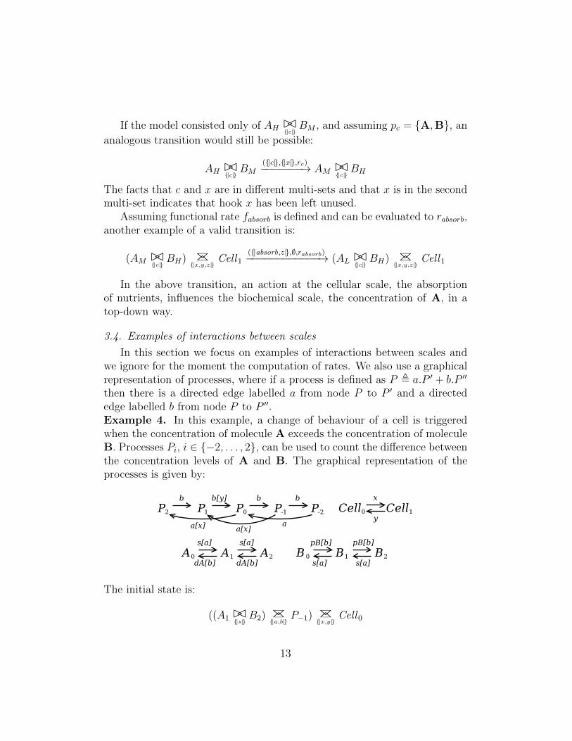
then there is a directed edge labelled a from node P to P ′ and a directededge labelled b from node P to P ′′.Example 4. In this example, a change of behaviour of a cell is triggeredwhen the concentration of molecule A exceeds the concentration of moleculeB. Processes Pi, i ∈ {−2, . . . , 2}, can be used to count the difference betweenthe concentration levels of A and B. The graphical representation of theprocesses is given by:

The initial state is:

((A1 BC{|s|} B2) BC

{|a,b|}P−1) BC

{|x,y|}Cell0

13

Species A can degrade (dA), B can be produced (pB), while both A and Bcan synchronise (on s) so that a level of B is converted into a level of A.Processes Pi, i ∈ {−2, . . . , 2}, represent the difference between the currentlevel of A and of B, while a and b actions represent events that make thisdifference increase by 2 and decrease by 1 respectively. An example transitionis:

((A1 BC{|s|} B2) BC

{|a,b|}P−1) BC

{|x,y|}Cell0

{|s,a,x|}[∅]−−−−−→ ((A2 BC{|s|} B1) BC

{|a,b|}P1) BC

{|x,y|}Cell1

Example 5. If a scale triggers more than one hook action, these hook actionscan be observed individually by multiple observers or together by a singleobserver. Consider the following processes:

Processes A0 and B1 can produce the following transition:

A0 BC{|s|} B1{|s|}[{|x,y|}]−−−−−−→ A1 BC{|s|} B0

In this case, two different instances of s synchronise, their set of hook actionsmerge in the resulting activity. Now consider the addition of processes P0,Q0 and R0. Two possible examples of transition are:

(A0 BC

{|x|}P0) BC

{|s|}(B1 BC

{|y|}Q0)

{|s,x,y|}[∅]−−−−−→ (A1 BC

{|x|}P1) BC

{|s|}(B0 BC

{|y|}Q1)

(A0 BC{|s|} B1) BC

{|x,y|}R0

{|s,x,y|}[∅]−−−−−→ (A1 BC{|s|} B0) BC

{|x,y|}R1

In the first transition, hook actions x and y are observed individually byprocesses P0 and Q0. If only hook action x were present, it would stillbe observed by P0 and the same for y with Q0. In the second transition,hook actions x and y are observed at the same time by process R0. Mostimportantly, we impose that R0 can synchronise only using the transition thatincludes the largest number of hooks available. In other words, transition{|x|}−−→ from R0 cannot synchronised with

{|s|}[{|x,y|}]−−−−−−→, because R0 can perform

14

{|x,y|}−−−→. This mechanism allows the modeller to design specific responses toevents that trigger multiple multi-scale events at the same time.Example 6. In some cases, a scale may trigger a multi-set of hook actions.Consider the following example. A cell contains three biochemical speciesA, B and C. The cell changes its behaviour if the biochemical scale reachesa specific configuration, that is when the concentrations of A and B arelow and when the concentration of C is high. Species A, B and C areproduced (actions pA, pB and pC ) and degrade (actions dA, dB and dC ) inthe cell. Finally, species A, B and C are involved in the biochemical reactionRs : A + B→ C. The model is defined as:

The initial state is:

((A1 BC{|s|} B1 BC{|s|} C1) BC

{|p,p,p,q|}P0) BC

{|x,y|}Cell0

Again we use processes Pi, i ∈ {0, . . . , 3}, to count the concentration requiredfor change at the cellular scale. In this particular case, a single transitioncan involve more than one identical hook action (i.e. p). The transition isthe following:

((A1 BC{|s|} B1 BC{|s|} C1) BC

{|p,p,p,q|}P0) BC

{|x,y|}Cell0

{|s,p,p,p,x|}[∅]−−−−−−−→

((A0 BC{|s|} B0 BC{|s|} C2) BC

{|p,p,p,q|}P3) BC

{|x,y|}Cell1

Another transition of the derivation graph generated by this model is:

((A2 BC{|s|} B1 BC{|s|} C1) BC

{|p,p,p,q|}P1) BC

{|x,y|}Cell0

{|s,p,p,x|}[∅]−−−−−−→

((A1 BC{|s|} B0 BC{|s|} C2) BC

{|p,p,p,q|}P3) BC

{|x,y|}Cell1

15

The multiplicity of the vertical cooperation set {|p, p, p, q|} is necessary. In

the above transition, the biochemical scale performs transition{|s|}[{|p,p|}]−−−−−−→,

while P1 can either perform transition{|p|}−−→ or

{|p,p|}[x]−−−−→. In order to choosethe correct transition, as seen in Example 5, we require that the multi-set ofactions from P1 is included in both the multi-set of hooks and the cooperationset, that is {|p, p|} ⊆ {|p, p|} ∩ {|p, p, p, q|}.

The use of multi-sets allows for a compact definition of this model, wherewe use the same action p to indicate that either A, B or C have reached theconcentration required for a change in behaviour of the cell.

Without multi-sets, an alternative definition of the same model is as fol-lows:

The above version of the model uses actions a, b and c in place of p creatinga combinatorial problem. As a result, the derivation graph of process P0

presents 19 transitions instead of nine.Example 7. The positioning of hook actions on actions at the biochem-ical scale is particularly useful when geometrical space is considered. LetAen denote the process representing a concentration level n of species A inregion Re. Concentration can migrate to and from region Re and many dif-ferent transport actions will have the same effect of lowering or increasing theconcentration of A in one region, as shown in the following diagram (onlyoutgoing transport shown):

16

The concentration of A is decreased, from Aen to Aen−1, through a transportaction of the form transp-es, s ∈ {b, d, f, h}. Correspondingly, at region Rs,the concentration of A increases, from Asm to Asm+1. If we want to denotethat a threshold is crossed when passing from level n to n − 1 of A at Re,we can add a hook action to the four transport actions, transp-es, obtainingtransp-es[y].Example 8. In this example we show how to abstract multiple regions toa single region, with respect to a specific property. Consider an area Rl of3 × 3 regions, labelled from Ra to Ri. We ignore detail of the biochemicalreactions, but assume that at some point each of these locations can becomeinfected, exposing hook action a, or they can recover, exposing hook actionb. We are not interested in which region has changed its status, only thenumber infected in Rl. A scale that represents the degree of infection of areaRl is defined by three processes, Rlow, Rmed and Rhigh.

Processes Pi, i ∈ {0, . . . , 9} are used to count the number of infected regions.If the number of infected regions is between 0 and 2, the degree of infectionis low; between 3 and 5 it is medium; larger than 5 it is high. Hooks x andy identify transitions between stages of infection.

3.5. Examples of Equivalences

Example 9. Consider the following processes:

17

Figure 4: Filtered transition graphs of the example in this section. If rd = ra + re = r thetransition systems are Markovian T -bisimilar.

A0 , a[b].A1 + e[b].A1 D0 , b[c].D1 A1 , nil D1 , nil

B0 , b[c].B1 E0 , d.E1 B1 , nil E1 , nil

C0 , d[b].C1 C1 , nil

Consider two PAH processes: A0 BC{|b|}

B0 and (C0 BC

{|b|}D0) BC

{|d|}E0. The following

transitions are possible:

A0 BC

{|b|}B0

({|a,b|}[c],∆)−−−−−−→ A1 BC{|b|}

B1

A0 BC

{|b|}B0

({|e,b|}[c],∆′′)−−−−−−−→ A1 BC{|b|}

B1

(C0 BC

{|b|}D0) BC

{|d|}E0

({|d,b|}[c],∆′)−−−−−−−→ (C1 BC{|b|}

D1) BC{|d|}

E1

These are the only possible transitions. We cannot consider the two processesequivalent in the sense that they generate isomorphic transition graphs, so

A0 BC

{|b|}B0 6≡ (C0 BC

{|b|}D0) BC

{|d|}E0. However, if we decide to select only actions

in the multi-set T = {|b|}, and rating yields rates ra, re and rd, we obtaintransitions:

A0 BC

{|b|}B0

({|b|},{|c|},ra)−−−−−−−→T A1 BC

{|b|}B1

A0 BC

{|b|}B0

({|b|},{|c|},re)−−−−−−−→T A1 BC

{|b|}B1

(C0 BC

{|b|}D0) BC

{|d|}E0

({|b|},{|c|},rd)−−−−−−−→T (C1 BC

{|b|}D1) BC

{|d|}E1

We call filtering the operation of selecting actions on labels and filtered tran-

sitions the resulting transitions. If rd = ra + re = r, both A0 BC

bB0 and

(C0 BC

{|b|}D0) BC

{|d|}E0 can move to a terminal state with filtered set of layer ac-

tions {|b|} and set of unused hook actions {|c|} with a total rate of r. Inother words, the pair ({|b|}, {|c|}) appears on an activity at the same timewith the same probability, implying the two model processes are Markovian

T -bisimilar, written A0 BC

{|b|}B0 'T (C0 BC

{|b|}D0) BC

{|d|}E0 (Figure 4). We will

demonstrate 'T is a congruence for process algebra with hooks processes.

18

4. Process Algebra with Hooks

A preliminary version of process algebra with hooks (PAH) has beenpublished in [31]. In this early work we followed a bottom-up approach wherethe biochemical scale determines the rates and other scales are abstractionsof lower scales. The current syntax and almost identical semantics were firstintroduced in [1], where we followed a middle-out [25] approach and whereone can begin modelling at any scale, and then relate to higher or lowerscales.

The syntax of PAH is:

D ::= nil | A[E ].A | D +D

M ::= A |M BCLM |M BC

LM

where:

• D is a definition process, D ∈ Pd, while M is a model process, M ∈ Pm.Definition and model processes are disjoint and are both processes, i.e.Pd ∪ Pm = P and Pd ∩ Pm = ∅, with P the set of processes;

• Agents are defined as A , D, that is we use definition processes todefine the behaviour of agents. This definition has to be unique foreach agent;

• a model is defined by a model process M , which in turn is either anagent A, a horizontal cooperation between model processes M BC

LM

or a vertical cooperation between model processes M BC

LM ;

• action execution A[E ].A is always followed by an agent A. This ensuresthat at any time the state of a model will be constituted of cooperationsof agents;

• functions Var(A) and Val(A) must be defined for each agent A, withVar(A) ∈ Names, Val(A) ∈ R and Names the set of parameter names;

• L, A and E are multi-sets of actions, with L = (L′,mL), A = (A′,mA)and E = (E ′,mE). Definitions of multi-sets and operations on multi-setsare given in Appendix A. Moreover, L′ ⊆ Actions, A′ ⊆ Actions∧A 6=∅, E ′ ⊆ Actions ∧ |E ′| ≤ 1, with Actions the set of actions;

19

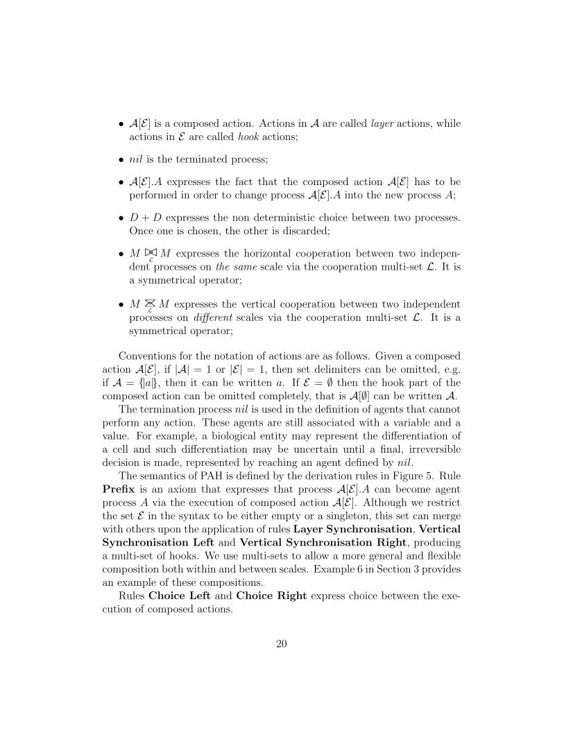
• A[E ] is a composed action. Actions in A are called layer actions, whileactions in E are called hook actions;

• nil is the terminated process;

• A[E ].A expresses the fact that the composed action A[E ] has to beperformed in order to change process A[E ].A into the new process A;

• D + D expresses the non deterministic choice between two processes.Once one is chosen, the other is discarded;

• M BCLM expresses the horizontal cooperation between two indepen-

dent processes on the same scale via the cooperation multi-set L. It isa symmetrical operator;

• M BC

LM expresses the vertical cooperation between two independent

processes on different scales via the cooperation multi-set L. It is asymmetrical operator;

Conventions for the notation of actions are as follows. Given a composedaction A[E ], if |A| = 1 or |E| = 1, then set delimiters can be omitted, e.g.if A = {|a|}, then it can be written a. If E = ∅ then the hook part of thecomposed action can be omitted completely, that is A[∅] can be written A.

The termination process nil is used in the definition of agents that cannotperform any action. These agents are still associated with a variable and avalue. For example, a biological entity may represent the differentiation ofa cell and such differentiation may be uncertain until a final, irreversibledecision is made, represented by reaching an agent defined by nil.

The semantics of PAH is defined by the derivation rules in Figure 5. RulePrefix is an axiom that expresses that process A[E ].A can become agentprocess A via the execution of composed action A[E ]. Although we restrictthe set E in the syntax to be either empty or a singleton, this set can mergewith others upon the application of rules Layer Synchronisation, VerticalSynchronisation Left and Vertical Synchronisation Right, producinga multi-set of hooks. We use multi-sets to allow a more general and flexiblecomposition both within and between scales. Example 6 in Section 3 providesan example of these compositions.

Rules Choice Left and Choice Right express choice between the exe-cution of composed actions.

20

Prefix Agent

A[E ].AA[E]−−→ A

DA[E]−−→ A′

A(A[E],∆)−−−−−→ A′

A , D∧ ∆ = {(Var(A),Val(A))}

Choice Left Asynchronous Left

D1A[E]−−→ A

D1 +D2A[E]−−→ A

M1(A[E],∆)−−−−−→M ′

1

M1 BCL M2(A[E],∆)−−−−−→M ′

1BCLM2

A ∩ L = ∅

Choice Right Asynchronous Right

D2A[E]−−→ A

D1 +D2A[E]−−→ A

M2(A[E],∆)−−−−−→M ′

2

M1 BCL M2(A[E],∆)−−−−−→M1 BCL M ′

2

A ∩ L = ∅

Layer Synchronisation

M1(A[E],∆1)−−−−−→M ′

1 M2(B[F ],∆2)−−−−−→M ′

2

M1 BCL M2(A∪B[E]F ],∆1∪∆2)−−−−−−−−−−−→M ′

1BCLM ′

2

A ∩ B ∩ L 6= ∅

Vertical Asynchronous Left

M1(A[E],∆)−−−−−→M ′

1

M1 BC

LM2

(A[E],∆)−−−−−→M ′1 BC

LM2

A ∩ L = ∅ ∧ E ∩ L = ∅

Vertical Asynchronous Right

M2(B[F ],∆)−−−−−→M ′

2

M1 BC

LM2

(B[F ],∆)−−−−−→M1 BC

LM ′

2

B ∩ L = ∅ ∧ F ∩ L = ∅

Vertical Synchronisation Left

M1(A[E],∆1)−−−−−→M ′

1 M2(B[F ],∆2)−−−−−→M ′

2

M1 BC

LM2

(A∪B[(E\B)]F ],∆1∪∆2)−−−−−−−−−−−−−−→M ′1 BC

LM ′

2

B ⊆ E ∩ L ∧ ¬(∃M2

(B′[F ′],∆′2)−−−−−−→M ′′

2 .(B′ ⊆ E ∩ L) ∧ (|B′| > |B|))

Vertical Synchronisation Right

M1(A[E],∆1)−−−−−→M ′

1 M2(B[F ],∆2)−−−−−→M ′

2

M1 BC

LM2

(A∪B[(F\A)]E],∆1∪∆2)−−−−−−−−−−−−−−→M ′1 BC

LM ′

2

A ⊆ F ∩ L ∧ ¬(∃M1

(A′[E ′],∆′1)−−−−−−→M ′′

1 .(A′ ⊆ F ∩ L) ∧ (|A′| > |A|))

Figure 5: Stochastic semantics of process algebra with hooks. Union of multi-sets isdenoted by ∪, while sum of multi-sets is denoted by ].

21

Rule Agent replaces definition processes with agent processes and con-structs environment ∆ using variables and values associated with agents.

Rule Layer Synchronisation is a weaker version of typical multi-waysynchronisation in process algebra. In fact, this rule can be applied evenif the labels of the transitions from processes M1 and M2 are not identi-cal: it is only required that multi-sets A and B share at least a name andthat this name is also in L. The resulting transition presents the multi-setunion of multi-sets of layer actions A and B, to represent the result of thesynchronisation. Conversely, multi-set sum of multi-sets of hooks E and Fis used to represent the collection of hooks summing the multiplicity of thehook actions. Moreover, partial functions ∆1 and ∆2 are merged assumingno clashing of variable names. In rules Asynchronous Left and Asyn-chronous Right, processes in cooperation can proceed asynchronously onlyif action set A does not share actions with cooperation set L.

The behaviour induced by the BC

Loperator is regulated by the rules Ver-

tical Synchronisation Left, Vertical Synchronisation Right, VerticalAsynchronous Left and Vertical Asynchronous Right. Rules differingin the name only by Left and Right are symmetric, so we explain only one ofthem. In Vertical Synchronisation Left, the synchronisation is betweenthe multi-set of hook actions on the left hand side (E) and the multi-setof layer actions on the right hand side (B), via actions in the cooperationmulti-set L. More specifically, some inter-scale actions in E are interpretedby another scale via B. For this to happen we impose in the side rule thatB must be included in both E and L. The resulting transition presents themulti-set union of multi-sets A and B, while B is subtracted from E to rep-resent the fact that some of the hook actions of the left hand side have beenused. Multi-set sum is used between E \ B and F to collect the remaininghook actions. It may be that more than one transition from M2 presents amulti-set of suitable layer actions B. In this case, we consider the largest Bmulti-sets, imposed by the side condition, which states that there is no othertransition from M2 which presents a multi-set of layer actions B′ included inboth E and L that is larger than B. This gives the possibility to the mod-eller to choose how the model should behave when multiple hook actions areoffered in a single transition (see Examples 5 and 6 in Section 3). Finally, inVertical Synchronisation Left we collect environments ∆1 and ∆2.

Consider now the inference rule Vertical Asynchronous Left. In thiscase, we allow a single process to transition asynchronously only if there are

22

no actions in the multi-set A which are also contained in L and no actionsin the hook multi-set E contained in L. This is because the actions in thevertical cooperation set L are hooks and if A ∩ L 6= ∅ (or E ∩ L 6= ∅)then A (or E) contains hooks and the transition is not intended to be usedasynchronously, but only with a suitable transition from M2.

We introduce now definitions necessary to define the derivation graph forPAH processes.

Definition 1. Activity. The pair (A[E ],∆) such that A, E ⊆ Actions and∆ ⊆ Names× R, with ∆ a partial function, is called an activity.

Definition 2. One step derivative. Given P ∈ P, if Pa−→ P ′ then P ′ is a

one step derivative of P . We denote the set of one step derivatives of P asosds(P ) = {P ′ | P a−→ P ′}.

Definition 3. Derivative. Given Mi ∈ Pm, If Mia−→ . . .

a′−→Mj then Mj is aderivative of Mi.

Definition 4. Derivative Set. The derivative set of a model process M ∈ Pmis denoted by ds(M) and is defined as the smallest set of model processessuch that:

• M ∈ ds(M);

• if Mi ∈ ds(M) and Mi(A[E],∆)−−−−−→Mj then Mj ∈ ds(M).

Definition 5. Current moves of a process. The multi-set of moves thatP ∈ P can perform is denoted by Moves(P ) and is defined as:

• (a, P ′) ∈ Moves(P ) iff Pa−→ P ′, with the same multiplicity as the

number of derivation trees that can derive Pa−→ P ′ using the derivation

rules in Figure 5.

Definition 6. Current activities for model Processes. The multi-set of ac-tivities that M ∈ Pm can perform is denoted by Activities(M) and is definedas:

Activities(M) = {|(A[E ],∆) | ((A[E ],∆),M ′) ∈Moves(M)|}

23

Definition 7. Activity set. The multi-set of activities that a model processM ∈ Pm and its derivatives can perform is given by:

−−−−−−→Activities(M) =

⊎Mi∈ds(M)

Activities(Mi)

Definition 8. Derivation graph. Given a model component M ∈ Pm, thederivation graph D(M) is the labelled directed graph with:

• set of nodes ds(M);

• multi-set of transition labels−−−−−−→Activities(M);

• multi-set of labelled transitions →⊆ ds(M)×−−−−−−→Activities(M)× ds(M).

Given M ′ ∈ ds(M), (M ′,A[E ],∆,M ′′) ∈→ with the same multiplicityas ((A[E ],∆),M ′′) in Moves(M ′).

4.1. Functional Rates

Functional rates are arithmetical expressions used to define rates of bi-ological events that are parametric with respect to the current state of thesystem. In order to do so, functional rates contain parameter names, thevalue of which depend on the environment ∆ in an activity (A[E ],∆) andon an additional environment Γ of constant model parameters. Functionalrates are associated with actions. Because we use sets of actions, in Section4.2 we introduce constraints that ensure that at most one functional rate isassociated with each transition. The syntax of functional rates is given by:

f ::= k | i | f binop f | unop(f)

binop ::= + | − | ∗ | / | ∧ unop ::= exp | log | sin | cos

• k ∈ R and i ∈ Names, i.e. i is a parameter name;

• f is a functional rate, f ∈ F;

• exp is the base e exponential operator;

• ∧ is the binary exponential operator.

24

The set F contains the functional rates defined in a PAH model, indexedby action names. For example, if fa ∈ F then fa is the functional rate associ-ated with action a. The evaluation of functional rates follows the standard se-mantics of arithmetical expressions. Given an environment ∆′ ⊆ Names×R,and a functional rate f , f evaluates to k ∈ R iff ∆′ ` f → k is valid. Inpractice, the environment ∆′ is the partial function obtained from the union∆′ = ∆ ∪ Γ of the environment of constant model parameters Γ and theenvironment ∆ in the activity to be rated.

4.2. PAH Model and Well-Formed PAH Model

We proceed now to the definition of a PAH model and well-formed PAHmodel.

Definition 9. PAH model. A PAH model is a tuple:

(AgentDef ,M,Actions,Names,F,Γ, Part,Var ,Val)

where:

• AgentDef is the finite set of agent definitions {A1 , D1, A2 , D2, . . . };

• M is the initial state of the model, with M ∈ Pm;

• Actions is the finite set of actions;

• Names is the finite set of parameter names;

• F is the finite set of functional rates;

• Γ is a partial function that associates parameters names with theirvalues, with Γ ⊆ Names× R. This partial function contains constantmodel parameters;

• Part is the finite set of sets of participants;

• Var and Val are the functions associating agents with variables (i.e.parameter names) and values, with Var : Pm → Names and Val :Pm → R.

25

In order to ensure a correct and unambiguous rate evaluation (Section 4.3)and to guarantee that congruence relations (Section 6.1) can be defined onPAH processes, we consider only well-formed PAH models, which are char-acterised as follows.

Definition 10. Well formed PAH model. A PAH model is well formed ifand only if:

1. each functional rate fa ∈ F is associated with a set of participantspa ⊆ Names:

∀a ∈ Actions, fa ∈ F⇔ pa ∈ Part

2. at any time only one agent can be associated with a certain variable.Given a model process as a cooperation of agents of the form

A1 ◦ A2 ◦ · · · ◦ An

then ∀Ai, Aj if i 6= j then Var(Aj) 6= Var(Aj), where ◦ is either avertical or horizontal cooperation;

3. whenever an agent A performs an action (application of derivation ruleAgent), the resulting agent A′ will be associated with the same variableA is associated with. Given a definition of an agent A as a choice ofprefix actions of the form

A ,∑i

ai.Ai

then ∀Ai Var(A) = Var(Ai);

4. if an agent A can perform activity (A[E ],∆) and A contains an actiona associated with a functional rate fa, then A = {|a|}. Moreover, if anaction is used as hook it cannot be associated with a functional rate.∀A agents defined as

A ,∑i

Ai[Hi].Ai

∀a s.t. fa ∈ F, if a ∈ Ai then Ai = {|a|} and ∀a s.t. fa ∈ F, a 6∈ Hi.

5. an agent A or one of its derivatives can perform action a if and only ifA is associated with a variable in pa. ∀a s.t. fa ∈ F, ∀A agents

∃E ,∆ s.t. (a[E ],∆) ∈−−−−−−→Activities(A)⇔ Var(A) ∈ pa

26

6. whenever M1 BCL M2 then M1 and M2 do not contain BC

L.

A well-formed PAH model implies the following propositions.

Proposition 11. Given a well-formed PAH model, at any time only oneagent is associated with a certain variable name, i.e. given M ∈ Pm initialstate of the PAH model, ∀M ′ ∈ ds(M), point 2 of Definition 10 holds.

Proof. This is follows from points 2 and 3 in Definition 10 and by the syntaxand semantics of PAH that ensure that given an initial state, no transitioncan increase or decrease the number of processes.

Proposition 12. Given a well-formed PAH model, environments ∆1 and ∆2

in L¯

ayer Synchronisation, Vertical Synchronisation Left and VerticalSynchronisation Right rules, always contain disjoint parameter names,ensuring no clashes of names in the union ∆1 ∪∆2, i.e. ∀i, j ∈ Names, with(i, k1) ∈ ∆1 and (j, k2) ∈ ∆2, then i 6= j.

Proof. This follows from Proposition 11.

Proposition 13. Given a well-formed PAH model with initial state M , in

each transition M ′ (A[E],∆)−−−−−→ M ′′ with M ′ ∈ ds(M), A contains at most oneaction associated with a functional rate.

Proof. This follows from points 4 and 6 in Definition 10. Given a composedaction A[E ], Point 4 in Definition 10, ensures that before any synchronisationis applied, if A contains a such that fa ∈ F, then A = {|a|}, while E cannotcontain actions associated with functional rates. The only way to add otheractions to A is via vertical synchronisation, because horizontal synchronisa-tion can happen only with other {|a|} multi-sets. The application of a verticalsynchronisation can only add to A actions that were previously in a hookmulti-set, and, by point 4 in Definition 10, are not associated with func-tional rates. After a vertical synchronisation, the only way to merge A witha different multi-set containing an action associated with a functional rate,would be to apply a horizontal synchronisation. However, this is impossiblebecause of point 6 in Definition 10.

Proposition 14. Given a well-formed PAH model, no more than |pa| agentscan synchronise via action a.

Proof. This follows from point 5 in Definition 10 and Proposition 11.

27

4.3. Rating PAH Activities

In this section we formalise the concepts of open and closed activities thatwe introduced in Section 3.2 as well as rating of PAH activities.

Formally, an activity (A[E ],∆) can be rated only if A contains exactlyone action name a such that fa ∈ F and ∆ contains the variables in pa. Suchactivity is called closed. An activity that is not closed is called open.

Additionally, when multiple transitions from a certain state are associatedwith the same functional rate we impose that the evaluated rate has to bedivided by the number of such transitions. This situation can arise as a resultof non-deterministic vertical synchronisations.

Definition 15. Current closed activities of a model process. Given a set offunctional rates F and a set of sets of participants Part, activity (A[E ],∆)is closed iff the following points are both true:

• there exists unique a s.t. a ∈ A and fa ∈ F;

• the corresponding pa ∈ Part is included in the variables in ∆.

Given a model process M ∈ Pm, the set of closed activities of M isdenoted by ClosedAct(M) and is defines as:

ClosedAct(M) ={∣∣∣∣(A[E ],∆)

∣∣∣∣ (A[E ],∆) ∈ Activities(M) ∧ ∃!a s.t. (a ∈ A∧fa ∈ F) ∧ (pa ∈ Part ∧ pa ⊆ {i|(i, k) ∈ ∆})

∣∣∣∣}Definition 16. Current open activities of a model process. Given a modelprocess M ∈ Pm, the multi-set of closed activities that M can perform isdefined as:

OpenAct(M) = Activities(M) \ ClosedAct(M)

Definition 17. Closed and open activity sets. The multi-sets of all closedand open activities that a model process M ∈ Pm can perform are definedas: −−−−−−−→

ClosedAct(M) =⊎

Mi∈ds(M)

ClosedAct(Mi)

−−−−−−→OpenAct(M) =

⊎Mi∈ds(M)

OpenAct(Mi)

28

Definition 18. Open moves of a model process. Given a model processM ∈ Pm, the multi-set of open moves of M , denoted OpenMoves(M), isdefined as:

OpenMoves(M) = {|(a,M ′) | (a,M ′) ∈Moves(M) ∧ a ∈ OpenAct(M))|}

Definition 19. Rated activity. The pair (A[E ], r) such that A, E ⊆ Actionsand r ∈ R>0 is called a rated activity.

Definition 20. Current rated activities of a model process. Given an envi-ronment of constant model parameters Γ ⊆ Names×R and a model processM ∈ Pm, the current set of rated activities of M is defined as:

RatedAct(M)Γ ={∣∣∣∣(A[E ], r)

∣∣∣∣ (A[E ],∆) ∈ ClosedAct(M) ∧ fa ∈ F ∧ a ∈ A∧ Γ ∪∆ ` fa → k ∧ r = k/π(ClosedAct(M), a)

∣∣∣∣}where π(A, a) returns the number of occurrences of (B[F ],∆′) in the multi-setA such that a ∈ B.

Definition 21. Rated activity set. Given an environment of constant modelparameters Γ ⊆ Names× R, the multi-set of rated activities that a modelprocess M ∈ Pm and its derivatives can perform is given by:

−−−−−−→RatedAct(M)Γ =

⊎Mi∈ds(M)

RatedAct(Mi)

−−−−−−→RatedAct(M)Γ can be written

−−−−−−→RatedAct(M) if Γ is clear from the context.

Definition 22. Rated moves of a model process. Given a model processM ∈ Pm and an environment of constant model parameters Γ ⊆ Names×R,the multi-set of rated moves of M , denoted RatedMoves(M)Γ, is defined as:

RatedMoves(M)Γ =

{∣∣∣∣((A[E ], r),M ′)

∣∣∣∣ ((A[E ],∆),M ′) ∈Moves(M)∧(A[E ], r) ∈ RatedAct(M)Γ

∣∣∣∣}Definition 23. Rated derivation graph. Given a model process M ∈ Pm andan environment of constant model parameters Γ ⊆ Names× R, the ratedderivation graph Dr(M)Γ is the labelled directed graph with:

29

• set of nodes ds(M);

• multi-set of transition labels−−−−−−→RatedAct(M)Γ;

• multi-set of labelled transitions→Γ⊆ ds(M)×−−−−−−→RatedAct(M)Γ×ds(M).

Given M ′ ∈ ds(M), (M ′,A[E ], r,M ′′) ∈→Γ with the same multiplicityas ((A[E ], r),M ′′) in RatedMoves(M ′)Γ.

• multi-set of labelled transitions →o⊆ ds(M)×−−−−−−→OpenAct(M)× ds(M).

Given M ′ ∈ ds(M), (M ′,A[E ],∆,M ′′) ∈→o with the same multiplicityas ((A[E ],∆),M ′′) in OpenMoves(M ′).

Dr(M)Γ can be written Dr(M) if Γ is clear from the context.

5. Relating Biological Systems to Aid Model Development

The development of PAH models can become overwhelming when anincreasing number of interactions between scales is considered. Ensuringconsistency of interactions between scales is an issue that affects multi-scalemodels in general, often requires manual checking and is specific to the modelat hand. But, in a process algebraic framework, there is an elegant solutionin the form of a relation that describes compatibility between scales and canbe applied to any PAH model.

In this section we introduce the compatibility L-bisimulation (�L), thatensures that two model processes can interact correctly via a vertical synchro-

nisation with cooperation set L (i.e. BC

L). Two processes interact correctly

when whenever one process can perform a composed action A[E ] with hooksE that are present in the cooperation set L, then the other process is able tosynchronise with that action. If the condition is not satisfied, then the twoscales are not compatibility L-bisimilar. There is an error in the definitionof the interactions between scales that the modeller needs to rectify.

In order to define this relation as bisimulation, we need to ensure thatevery transition the first process can perform is matched by transitions ofthe second and vice versa.

Before we can give a formal definition of compatibility L-bisimulation, weneed to define:

• a new transition symbol⇒L, which stands for zero or more transitionsthat do not contain any action in L. We use this to ignore transitions

30

that are not involved with the vertical syncronisation we want to check.This is analogous to the approach used in weak bisimulation to ignoreτ actions [17];

• a notion of transitions safely blocked, that cannot synchronise via ver-tical cooperation and that can be ignored. When two model processes

M1 and M2 are put in parallel with BC

L, some of the transitions

(A[E],∆)−−−−−→that M1 or M2 alone can perform become blocked. There are two rea-sons why this occurs. The former is that A∩L 6= ∅ and synchronisationcannot take place because the other process cannot immediately pro-duce the necessary hooks. These are the safely blocked transitions. Thelatter is that E ∩L 6= ∅ and synchronisation cannot take place becausethe other process cannot “respond” to the hooks present in E ∩ L. Ifthis is the case, then M1 6�L M2, so we exclude this case from thedefinition of compatibility L-bisimulation.

Formal definitions are given below. Because in this section we are not

interested in environments and rates, we use M1A[E]−−→ M2 to imply ∃∆.

M1(A[E],∆)−−−−−→M2.

Definition 24. Transition ⇒L. Given M1,M2 ∈ Pm, M1 ⇒L M2 iff:

• M1 = M2 or

• M1A1[E1]−−−→ ...

Ai[Ei]−−−→ ...An[En]−−−−→ M2 and ∀i = 1, ..., n, Ai ∩ L = ∅ and

Ei ∩ L = ∅

Definition 25. Transition safely blocked by a model process via a cooper-ation set. Given model processes M1,M2 ∈ Pm and a cooperation set

L ⊆ Actions, a transition M1A[E]−−→ M ′

1 is safely blocked by M2 via L iffA ∩ L 6= ∅ and:

• ¬(∃M ′2. M2

B[F ]−−→M ′2 with A ⊆ F ∩ L) or

• ∃M ′2. M2

B[F ]−−→ M ′2 with A ⊆ F ∩ L and ∃M ′′

1 . M1A′[E ′]−−−→ M ′′

1 withA′ ⊆ F ∩ L and |A′| ≥ |A|

31

Definition 26. Compatibility L-bisimulation. A relation R ⊆ Pm × Pmis a compatibility L-bisimulation iff whenever (M1,M2) ∈ R then for all

M1A[E]−−→ M ′

1 that are not safely blocked by M2 via L we have one of thefollowing:

• if A ∩ L = ∅ ∧ E ∩ L = ∅ then ∃M ′2. M2 ⇒L M ′

2 and (M ′1,M

′2) ∈ R;

• if A ∩ L 6= ∅ then ∃M ′2. M2

B[F ]−−→ M ′2 with A ⊆ F ∩ L) and ¬(∃M ′′

1 .

M1A′[E ′]−−−→M ′′

1 with A′ ⊆ F ′ ∩ L and |A′| ≥ |A|) and (M ′1,M

′2) ∈ R;

• if E ∩ L 6= ∅ then ∃M ′2. M2

B[F ]−−→ M ′2 with B ⊆ E ∩ L and ¬(∃M ′′

2 .

M2B′[F ′]−−−→M ′′

2 with |B′| ≥ |B|) and (M ′1,M

′2) ∈ R.

In addition, the same must be true for all M2B[F ]−−→ M ′

2 that are not safelyblocked by M1 via L.

Model processesM1 andM2 are compatibility L-bisimilar, denotedM1 �LM2, if (M1,M2) ∈ R for a compatibility L-bisimulation R.

5.1. Example of Use of Compatibility L-Bisimulation

In this section we propose a simple model of tissue growth. This modelis based on a more complex model of tissue growth that we presented in ourprevious work [1].

At the tissue scale we consider an area divided into regions of the samesize and shape. Without loss of generality, we consider only two regions, R1and R2 (Figure 6). Each region can be empty (agents beginning with E)or contain tissue. There are two types of tissue: active and inactive. Activetissue (agents beginning with Ton) is mitosis enabled (can perform actionsbeginning with mito), that is its cells can duplicate and produce tissue thatwill occupy a neighbouring empty region. Action mito12 represents, forexample, growth from region R1 to region R2 . If no adjacent region isempty, mitosis is inhibited. Inactive tissue (agents beginning with Toff )cannot replicate. Both types of tissue can become empty space throughapoptosis (actions beginning with apo), that is cell death.

The biochemical scale consists only of a biochemical species A, presentin the two regions. The concentration of A (agents beginning with A) canassume three possible values: low, medium and high (agents with subscriptL, M and H). Concentration level can change because of transport between

32

Figure 6: A theoretical multi-scale model of tissue growth.

regions (actions beginning with t, such as t12 for transport from region R1to region R2 ).

The following constraints, which require communication between scales,must hold:

• tissue is active in a region if and only if the concentration of A in thesame region is high. Hook actions beginning with mitoon and mitooffshould ensure this is the case;

• a region is empty if and only if there is no biochemistry. To representthe absence of biochemistry we use processes beginning with NA. Hookactions beginning with bioon and biooff should ensure this is the case.

Agent definitions are given below, with a graphical representation illus-trated in Figure 7:

NA1 , bioon1 .A1L E1 , mito21 [bioon1 ].Toff1

A1L , biooff1 .NA1 + t21 .A1M Toff1 , apo1 [biooff1 ].E1

A1M , biooff1 .NA1 +mitoon1 .Ton1

+t21 [mitoon1 ].A1H + t12 .A1L Ton1 , apo1 [biooff1 ].E1

A1H , biooff1 .NA1 +mito12 .Ton1+t12 [mitooff1 ].A1M +mitooff1 .Toff1

NA2 , bioon2 .A2L E2 , mito12 [bioon2 ].Toff2

A2L , biooff2 .NA2 + t12 .A2M Toff2 , apo2 [biooff2 ].E2

A2M , biooff2 .NA2 +mitoon2 .Ton2

+t12 [mitoon2 ].A2H + t21 .A2L Ton2 , apo2 [biooff2 ].E2

A2H , biooff2 .NA2 +mito21 .Ton2+t21 [mitooff2 ].A2M +mitooff2 .Toff2

33

Figure 7: Graphical representation of the processes defined in the tissue growth example.

The initial state of this model is (A1H BCL

NA2 ) BC

L′(Ton1 BC

L′′E2 ), where

L = {t12, t21}, L′ = {bioon1 , bioon2 , biooff1 , biooff2 , mitoon1 , mitoon2 ,mitooff1 , mitooff2} and L′′ = {mito12 , mito21}.

An example of transition is:

(A1H BCL

NA2 ) BC

L′(Ton1 BC

L′′E2 )

{mito12 ,bioon2}[∅]−−−−−−−−−−→(A1H BC

LA2L) BC

L′(Ton1 BC

L′′Toff2 )

In the above transition, action mito12 represents growth of tissue from regionR1 to region R2 , while vertical synchronisation with action bioon2 ensuresthat the biochemical scale in region R2 is enabled. It can be shown that

A1H BCL

NA2 �L′ Ton1 BCL′′

E2 .An example of a safely blocked transition is:

Ton1 BCL′′

E2mitooff1−−−−→ Toff1 BC

L′′E2

The above transition is safely blocked by A1H BCL

NA2 via L′. This is be-cause in this model the only way to reduce the concentration of A is bytransport from R1 to R2 , while such transport is not possible because NA2

34

represents the absence of biochemistry and cannot produce any transition

that can synchronise with A1Ht12 [mitooff1 ]−−−−−−−→ A1M .

Detect incorrect model definitions. We give now an example of a mis-take in the model definition that leads to non compatibility L-bisimilar pro-cesses. We show that by replacing process definition E2 , mito12 [bioon2 ].Toff2with E2 , mito12 .Toff2 , that is “forgetting” to place hook bioon2 , then

A1H BCL

NA2 6�L′ Ton1 BCL′′

E2 .After the replacement, following the definition of compatibility L-bisimula-

tion, transition

Ton1 BCL′′

E2mito12−−−−→ Ton1 BC

L′′Toff2

is matched by

A1H BCL

NA2 ⇒L′ A1H BCL

NA2

However, transition

Ton1 BCL′′

Toff2apo2 [biooff2 ]−−−−−−−→ Ton1 BC

L′′E2

cannot be matched by any transition from A1H BCL

NA2 . This implies

A1H BCL

NA2 6�L Ton1 BCL′′

Toff2 , which in turn implies A1H BCL

NA2 6�L′Ton1 BC

L′′E2 .

6. Relating Biological Systems at Specified Scales

In this section we define a relation that will allow us to:

• compare the behaviour of two different process algebra models withrespect to a specified scale;

• substitute parts of a model with behaviourally equivalent and less com-plex ones.

In particular, we define Markovian T -bisimulation ('T ), which ensures thattwo processes produce the same rated and filtered activities at the same timeand with the same probability, while presenting identical open transitions.

We anticipate that such relation may be too strong for most biologicalapplications. Nonetheless, such a relation is a fundamental relation from

35

which other relations can be defined. In particular, in biology one is ofteninterested in determining whether two systems are almost rather than exactlythe same, and possibly to which extent they are similar. We will discuss thisagain in Section 10.1.

In order to relate models at a specified scale, we define a mechanism tofocus on a specified scale in PAH. This mechanism is called filtering andconsists of removing undesired action names from valid rated transitionsbelonging to a rated derivation graph. The result will be a filtered derivationgraph. Because actions are associated with functional rates, removing actionsinterferes with rating. As a consequence, rating of transitions should alwaysprecede filtering.

In PAH actions from every scale are collected into a unique action multi-set that labels valid transitions. If we want to focus on a specific scale, allwe need to do is to keep only the actions pertaining to a given scale. Forexample, consider the following rated transition:

M({|a,h,x|}[{|y,z|}],r)−−−−−−−−−−→Γ M

′

From this transition it is possible to infer that actions a, h and x havebeen performed, that hook actions y and z have not been used in any syn-chronisation and that the rate of the transition is r. Now assume that weare interested in only the behaviour represented by the actions in T , withT = {|x, y|}. The corresponding filtered transition should be:

M({|x|},{|y,z|},r)−−−−−−−−→T ,Γ M ′

Notice that the rate and the multi-set of hook actions is untouched. More-over, a filtered activity is a triple, to distinguish it from a rated activity,which is a pair. We introduce now the formal definitions of filtered activities,filtered transitions and filtered derivation graph.

Definition 27. Filtered activities. The triple (A, E , r) such that A and Eare multi-sets of actions and r ∈ R>0 is called a filtered activity.

Definition 28. Current filtered activities of a model process. Given a multi-set of actions T and an environment Γ ⊆ Names × R, the multi-set offiltered activities that a model process M ∈ Pm can perform is denoted byFiltAct(M)T ,Γ and is defined as:

FiltAct(M)T ,Γ = {|(B, E , r) | (A[E ], r) ∈ RatedAct(M)Γ ∧ B = A ∩ T |}

36

Definition 29. Filtered activity set. Given a multi-set of actions T and anenvironment Γ ⊆ Names×R, the multi-set of filtered activities that a model

process M ∈ Pm and its derivatives can perform is denoted by−−−−−→FiltAct(M)T ,Γ

and is defined as:−−−−−→FiltAct(M)T ,Γ =

⊎Mi∈ds(M)

FiltAct(Mi)T ,Γ

Definition 30. Filtered moves of a definition process. Given a multi-setof actions T , the multi-set of moves that a definition process D ∈ Pd canperform is denoted by FiltMovesDT and is defined as:

FiltMoves(D)T = {|((B, E), A) | (A[E ], A) ∈Moves(D) ∧ B = A ∩ T |}

Definition 31. Filtered moves of a model process. Given a multi-set of ac-tions T and an environment Γ ⊆ Names × R, the multi-set of moves thata model process M ∈ Pm can perform is denoted by FiltMovesMT ,Γ and isdefined as:

FiltMoves(M)T ,Γ =

{∣∣∣∣((B, E , r), A)

∣∣∣∣ ((A[E ], r), A) ∈ RatedMoves(M)Γ

∧B = A ∩ T

∣∣∣∣}Definition 32. Filtered derivation graph. Given a model process M ∈ Pm,a multi-set of actions T and an environment Γ ⊆ Names× R, the filteredderivation graph Df (M)T ,Γ is the labelled directed graph with:

• set of nodes ds(M);

• multi-set of transition labels−−−−−→FiltAct(M)T ,Γ;

• multi-set of labelled transitions→T ,Γ⊆ ds(M)×−−−−−→FiltAct(M)T ,Γ×ds(M).

Given M ′ ∈ ds(M), (M ′,A, E , ra,M ′′) ∈→T ,Γ with the same multiplic-ity as ((A, E , ra),M ′′) in FiltMoves(M ′)T ,Γ.

• multi-set of labelled transitions →o⊆ ds(M)×−−−−−−→OpenAct(M)× ds(M).

Given M ′ ∈ ds(M), (M ′,A[E ],Γ′,M ′′) ∈→o with the same multiplicityas ((A[E ],Γ′),M ′′) in OpenMoves(M ′).

Df (M)T ,Γ can be written Df (M) if T and Γ are clear from the context.

With the notion of filtered derivation graph we can now define relationsbetween PAH processes based on filtering and relate PAH processes at spec-ified scales.

37

6.1. Markovian (T ,Γ)-bisimulation

In this section we define formally Markovian (T ,Γ)-bisimulation ('T ,Γ)on PAH processes. The definition is based on strong equivalence in PEPA [29]and integrated equivalence in EMPA [32]. Two PAH processes are consideredMarkovian (T ,Γ)-bisimilar if it is possible to group the states of their filteredderivation graphs into equivalence classes in such a way that states belongingto the same equivalence class are characterised as follows:

• the sum of the rates of rated moves presenting the same action sets froma state in an equivalence class toward the states of another equivalenceclass is the same for all states in the same equivalence class;

• the set of open moves from a state in an equivalence class toward thestates of another equivalence class is the same for all states in the sameequivalence class.

In addition we prove that 'T ,Γ is an equivalence relation (Proposition 37)and a congruence (Proposition 40).

Definition 33. Functions µT ,Γ and νT ,Γ. Function µT ,Γ returns the rate rat which a model process M can become M ′ with filtered transitions labelledwith (A, E). Function νT ,Γ returns instead the rate at which M can move toa set of model processes C with filtered transitions labelled with (A, E).

µT ,Γ(M,A, E ,M ′) =∑ri∈I

ri

where I = {|r | ((A, E , r),M ′) ∈ FiltMoves(M)T ,Γ|}. For each rate r, thesame multiplicity as ((A, E , r),M ′) in FiltMoves(M)T ,Γ is used.

νT ,Γ(M,A, E , C) =∑M ′∈C

µT ,Γ(M,A, E ,M ′)

Definition 34. Open Activities toward a set of model processes. The multi-set of activities toward a set of model processes C ⊆ Pm of a model processM ∈ Pm is defined as:

OpenAct(M, C) = {|(A[E ],∆) | ((A[E ],∆),M ′) ∈ OpenMoves(M)∧M ′ ∈ C|}

38

Definition 35. Model process Markovian (T ,Γ)-bisimulation. Given an ac-tion multi-set T and an environment Γ ⊆ Names×R, an equivalence relationover model processes R ⊆ Pm × Pm is a model process Markovian (T ,Γ)-bisimulation iff whenever (M1,M2) ∈ R then ∀ action multi-sets A and Eand ∀C ∈ Pm/R

νT ,Γ(M1,A, E , C) = νT ,Γ(M2,A, E , C)

andOpenAct(M1, C) = OpenAct(M2, C)

Definition 36. Model process Markovian (T ,Γ)-bisimilarity. Model processMarkovian (T ,Γ)-bisimilarity, denoted 'T ,Γ, is the union of all model processMarkovian (T ,Γ)-bisimulations, i.e.

'T ,Γ=⋃{R | R is a model process Markovian (T ,Γ)-bisim.}

Two model processes M1,M2 ∈ Pm are Markovian (T ,Γ)-bisimilar, de-notedM1 'T ,Γ M2, iff there is a model process (T ,Γ)-bisimulationR betweenthem such that (M1,M2) ∈ R.

If Γ is clear from the context, we write M1 'T M2 instead of M1 'T ,Γ M2

and we say M1 and M2 are Markovian T -bisimilar.

Proposition 37. Model process Markovian (T ,Γ)-bisimilarity ('T ,Γ) is anequivalence relation and it is the largest model process Markovian (T ,Γ)-bisimulation.

Proof. A model process Markovian (T ,Γ)-bisimilarity is an equivalencerelation iff it is symmetric, reflexive and transitive. The first two propertiesare trivially true. We prove transitivity and at the same time we concludethat 'T ,Γ is the largest model process Markovian (T ,Γ)-bisimulation. Wefollow the same strategy as in [29].

We prove that given any number of bisimulationsRi, one can always find abisimulation that contains them all, which is given by the transitive closureof their union R = (

⋃iRi)

∗. Assume Ri is a model process Markovian(T ,Γ)-bisimulation for all i ∈ I. By definition, each Ri is an equivalencerelation that partitions Pm into equivalence classes. By definition of transitiveclosure, any equivalence class Sij ∈ Pm/Ri is included in some Tk ∈ Pm/R,with Tk =

⋃j S

ij and j ∈ J ik. The set J ik indicates how the equivalence classes

39

induced by Ri are merged into the equivalence class Tk. A bisimulation Ri′

might partition Tk in a different way, but because of the transitive closureTk =

⋃j S

ij =

⋃j′ S

i′

j′ , j′ ∈ J i′k . We now prove by induction on the definition of

transitive closure that R is a model process Markovian (T ,Γ)-bisimulation.Base: we define Rn = (

⋃iRi)

n, that is the n-th step in the expansionof the transitive closure. Consider R0 =

⋃iRi. If (M1,M2) ∈ R0 then

(M1,M2) ∈ Ri for some i ∈ I. This implies that for all action multi-sets Aand E and ∀Tk ∈ Pm/R:

νT ,Γ(M1,A, E , Tk) = νT ,Γ(M1,A, E ,⋃j∈Ji

k

Sij) =∑j∈Ji

k

νT ,Γ(M1,A, E , Sij)

=∑j∈Ji

k

νT ,Γ(M2,A, E , Sij) = νT ,Γ(M2,A, E , Tk)

and

OpenAct(M1, Tk) = OpenAct(M1,⋃j∈Ji

k

Sij) =⊎j∈Ji

k

OpenAct(M1, Sij)

=⊎j∈Ji

k

OpenAct(M2, Sij) = OpenAct(M2, Tk)

Induction: Given any (M1,M2) ∈ Rn−1 we assume that νT ,Γ(M1,A, E , Tk) =νT ,Γ(M2,A, E , Tk) and OpenAct(M1, Tk) = OpenAct(M2, Tk). We then provethat this is the case also for any (M ′

1,M′2) ∈ Rn. If (M ′

1,M′2) ∈ Rn then,

by definition of transitive closure, either (M ′1,M

′2) ∈ Rn−1 or (M ′

1,M′2) ∈

{(P,Q) | ∃R. (P,R) ∈ Rn−1 ∧ (R,Q) ∈ Rn−1}. This implies ∃R such that:

νT ,Γ(M ′1,A, E , Tk) = νT ,Γ(R,A, E , Tk) = νT ,Γ(M ′

2,A, E , Tk)

andOpenAct(M ′

1, Tk) = OpenAct(R, Tk) = OpenAct(M ′2, Tk)

This proves that given any number of model process Markovian (T ,Γ)-bisimulations, we can always find a bisimulation that contains them. Because'T ,Γ includes all possible bisimulations, then 'T ,Γ is at least as large as thelargest model process Markovian (T ,Γ)-bisimulation.

Definition 38. Filtered composed actions toward a set of model processes.Given a multi-set of actions T , the multi-set of composed actions toward aset of model processes C ⊆ Pm of a definition process D ∈ Pd is defined as:

FiltCompAct(D, C)T = {|(A, E) | ((A, E), D′) ∈ FiltMoves(D)T ∧D′ ∈ C|}

40

Definition 39. Markovian (T ,Γ)-bisimilar definition processes. Given anaction multi-set T and an environment Γ ⊆ Names×R, two definition pro-cessesD1, D2 ∈ Pd are definition process Markovian (T ,Γ)-bisimilar (D1 'T ,ΓD2) iff ∀C ∈ Pm/ 'T ,Γ

FiltCompAct(D1, C)T = FiltCompAct(D2, C)TProposition 40. Markovian (T ,Γ)-bisimulation as a Congruence. If P1, P2 ∈P such that P1 'T ,Γ P2, then

1. A[E ].P1 'T ,Γ A[E ].P2, with P1, P2 agents2. P1 +Q 'T ,Γ P2 +Q, with P1, P2, Q ∈ Pd3. P1 BCL Q 'T ,Γ P2 BCL Q, with P1, P2, Q ∈ Pm4. P1 BC

LQ 'T ,Γ P2 BC

LQ, with P1, P2, Q ∈ Pm

Proof. See Appendix B.

7. Parametric Stochastic Process Algebra with Hooks

In analogy with our previous work [1], in this section we introduce thesyntax of a parametric version of PAH. This version is equivalent to PAH asintroduced in the previous sections while it makes models easier to write andcomprehend because we can, in fact, index processes.

In general, we expect the modeller to develop his own scripts, for examplein a BASH environment, to produce automatically models that include hun-dreds of processes. The definition of these scripts goes beyond the scope ofthis paper and, in any case, the scripts would be tailored around the specificproblem modelled. For example, a script for a model of tissue growth wouldproduce automatically a grid of processes representing discrete portions oftissue. To check that the produced model is as intended, one can define re-lations such as our compatibility L-bisimulation (Section 5) and implementalgorithms to check whether these relations hold.

Here we limit ourselves to augmenting PAH as defined in Section 4 withparametrised processes and actions and we obtain a parametric stochasticprocess algebra with hooks (psPAH). The syntax of psPAH is as follows:

D ::= nil | A[E ].A(exp, . . . , exp) | D +D | if bexp then D else D

M ::= A(k, . . . , k) |M BCLM |M BC

LM

exp ::= k | i | exp+ exp | exp− exp | exp/exp | exp ∗ expbexp ::= exp = exp | exp < exp | bexp ∧ bexp |

bexp ∨ bexp | ¬bexp | true | false

41

The main differences between this and the non parametric version are:

• k ∈ R and i is a parameter name, i.e. i ∈ Names;

• actions have the form a(exp, . . . , exp), where exp, . . . , exp is a list ofexpressions. In particular, multi-sets L = (L′,mL), A = (A′,mA)and E = (E ′,mE), where A′, E ′ ⊆ Actions and L′ ⊆ ConstActions .Actions = {a(expa1, . . . , expan), b(expb1, . . . , expbn), . . . } andConstActions ⊂ Actions, ConstActions = {a(ka1, . . . , kan), b(kb1, . . . , kbn),. . . };

• a definition process can also be an if-then-else construct: if bexp thenD else D;

• agent definitions have now the form A(i1, . . . , in) , D, where i1, . . . , inis a list of parameter names;

• the evaluation of the expressions is performed when inference ruleAgent is applied;

• the definitions of functional rates and the variables associated withagents are also parametric.

The semantics is given in Figure 8. Given an environment ∆, the evalu-ation of an expression exp into a real number k is denoted by ∆ ` exp→ k,the evaluation of a boolean expression bexp into b ∈ {true, false} is denotedby ∆ ` bexp → b, while the evaluation of the list of expressions of all theactions in a set A is denoted by ∆ ` A → A′, where A′ contains only actionswith evaluated expressions.

An interpreter for psPAH has been implemented in the functional pro-gramming language OCaml. The interpreter reads as input the descriptionof a psPAH model along with a model time threshold for the simulations.Simulations are performed on a model, producing traces of states and timedelays using a standard sampling method for continuous time Markov chains.

Simulations have been performed on a laptop computer with UbuntuLinux, two Intel Core 2 Duo 2.20 GHz CPUs and 2 GB of RAM.

The simulations given in the next section, were all computed in within atmost 48 hours.

42

Prefix

A[E ].A(exp1, . . . , expn)A[E],true−−−−−→ A(exp1, . . . , expn)

Choice Left Choice Right

D1A[E],b−−−→ A(exp1, . . . , expn)

D1 +D2A[E],b−−−→ A(exp1, . . . , expn)

D2A[E],b−−−→ A(exp1, . . . , expn)

D1 +D2A[E],b−−−→ A(exp1, . . . , expn)

If Then Else True

D1A[E],b−−−→ A(exp1, . . . , expn)

if bexp then D1 else D2A[E],b∧bexp−−−−−−→ A(exp1, . . . , expn)

If Then Else False

D2A[E],b−−−→ A(exp1, . . . , expn)

if bexp then D1 else D2A[E],b∧¬bexp−−−−−−−→ A(exp1, . . . , expn)

Agent

DA[E],b−−−→ A′(exp1, . . . , expn)

A(k1, . . . , kn)(A′[E ′],∆′)−−−−−−→ A′(k′1, . . . , k

′n)

*

*if A(i1, . . . , in) , D ∧∆ = {(i1, k1), . . . , (in, kn)} ∧∆ ` b→ true∆ ` exp1 → k′1 ∧ · · · ∧∆ ` expn → k′n ∧∆ ` A → A′ ∧∆ ` E → E ′∧ ∆′ = {(Var(A(k1, . . . , kn)), V al(A(k1, . . . , kn)))}

Figure 8: Semantics of parametric stochastic process algebra with hooks. Other inferencerules are as in Figure 5.

8. Multi-Scale Model of Pattern Formation

We now give an example specification and analysis of a well-known prob-lem from Systems Biology: the French Flag problem [33]. In this well-knownsystem, a group of identical cells in a tissue are differentiated into subgroups,according to the diffusion of a morphogen.

A morphogen M diffuses from a source into a tissue. In the long run,the region close to the source presents a high concentration of M, while thefurther a region is from the source, the lower the concentration of M is inthat region. The concentration of M in a region indicates the positionalinformation, i.e. the position with respect to the source. Different specialisa-

43

0

0.2

0.4

0.6

0.8

1

0 0.5 1 1.5 2 2.5 3

concentr

ation

position

The French Flag Model

threshold 1

threshold 2

R1 R2 R3

Figure 9: The French Flag Model implemented with partial differential equations. In thepicture, two concentration thresholds divide the space into three regions.

tions are assigned to a region depending on the concentration of M in thatregion. Of great importance are concentration thresholds that delimit theconcentration ranges associated with different specialisations.

One of the simplest models of this scenario is the following partial differ-ential equation (PDE) [34]:

∂M(t, x)

∂t= D

∂2M(t, x)

∂x2− αM(t, x)

The above equation models the concentration of M in time and space in

one-dimensional coordinates. The element D∂2M(t, x)

∂x2is the diffusion of

M, while αM(t, x) is its degradation. Constant D is the diffusion constantand α is the degradation constant; we assume these two constants to be equalto 1. Boundary conditions are:

1. M(t, 0) = 1 with 0 ≤ t <∞, i.e. a constant source of M at position 0;2. M(t,∞) = 0 with 0 ≤ t < ∞, i.e. concentration of M is lost in the

surroundings.

Steady state solution of the PDE model is shown in Figure 9. In the figure,the steady state solution is shown (continuous line). Two concentration

44

Figure 10: Discretisation of the space of the French Flag Model into 20 regions. Thevariable M(i) indicates the concentration of M in region i.

thresholds (at 0.2 and 0.5, dotted lines) divide the area in three regions(R1, R2 and R3). Each of these regions are characterised by a differentspecialisation.

We propose now a representation of the PDE model in psPAH. Becausethe PDE model is continuous in the concentration of M and in space, whilepsPAH uses a discrete representation of these quantities, we provide a dis-cretisation. We assume 20 levels for the concentration of M (parametermaxLevels = 20), with maximum concentration equal to 1 and concentra-tion of each level equal to h = 1/20 = 0.05, and we assume 20 regions ofspace (parameter regions = 20), with total length equal to 3 and length ofeach region equal to deltaX = 3/20 = 0, 15. The spatial discretisation isillustrated in Figure 10.

In order to represent the two boundary conditions we have:

• the left most region presents a constant concentration level of 20, whichguarantees that concentration flows continuously from the left;

• the right most region presents a constant concentration level equal to0, which implies that this region absorbs concentration levels.

We define agentM(i, w) (Figure 11) to indicate that morphogen M in region ipresents concentration level w. Actions t(i, j) represent transport of M fromregion i to region j, while actions deg(i) represent degradation of M in regioni.

We model specialisation of regions explicitly as follows. Two thresholdsare considered: one between 4 and 5 concentration levels and the other be-tween 10 and 11. Whenever a concentration threshold is crossed in a region,the specialisation of the region changes. The presence of two thresholds im-plies that three specialisations are possible, corresponding to high, mediumand low concentration ranges of M. In addition, we consider that regions of

45

M(i, w) ,if i == 1 then //first region, the source of M

t(1, 2).M(1, w)else

if i == regions then //last region, absorbingt(regions− 1, regions).M(regions, w)

else //any other regionif w > 0 then //degradation of M

if w == (thr1 + 1) ∨ w == (thr2 + 1) thendeg(i)[y(i)].M(i, w − 1)

elsedeg(i).M(i, w − 1)

elsenil

+ //transport of M to next regionif i < regions ∧ w > 0 then

if w == (thr1 + 1) ∨ w == (thr2 + 1) thent(i, i + 1)[y(i)].M(i, w − 1)

elset(i, i + 1).M(i, w − 1)

elsenil

+ //transport of M from next regionif i < (regions− 1) ∧ w < maxLevels then

if w == (thr1) ∨ w == (thr2) thent(i + 1, i)[x(i)].M(i, w + 1)

elset(i + 1, i).M(i, w + 1)

elsenil

+ //transport of M to previous regionif i > 2 ∧ w > 0 then

if w == (thr1 + 1) ∨ w == (thr2 + 1) thent(i, i− 1)[y(i)].M(i, w − 1)

elset(i, i− 1).M(i, w − 1)

elsenil

+ //transport of M from previous regionif i > 1 ∧ w < maxLevels then

if w == (thr1) ∨ w == (thr2) thent(i− 1, i)[x(i)].M(i, w + 1)

elset(i− 1, i).M(i, w + 1)

elsenil

T (i, z, w) ,if w < 2 then

x(i).T (i, 0, w + 1)else

nil+if w > 0 then

(y(i).T (i, 0, w − 1)+if z < 1 then

mem(i).T (i, z + 1, w)else

if w == 2 thenmem(i).TA(i)

elsemem(i).TB(i)

elsenil

TA(i) , nil

TB(i) , nil

Figure 11: Agent definitions of processes M(i, w), T (i, z, w), TA(i) and TB(i), from themulti-scale model of pattern formation.

46

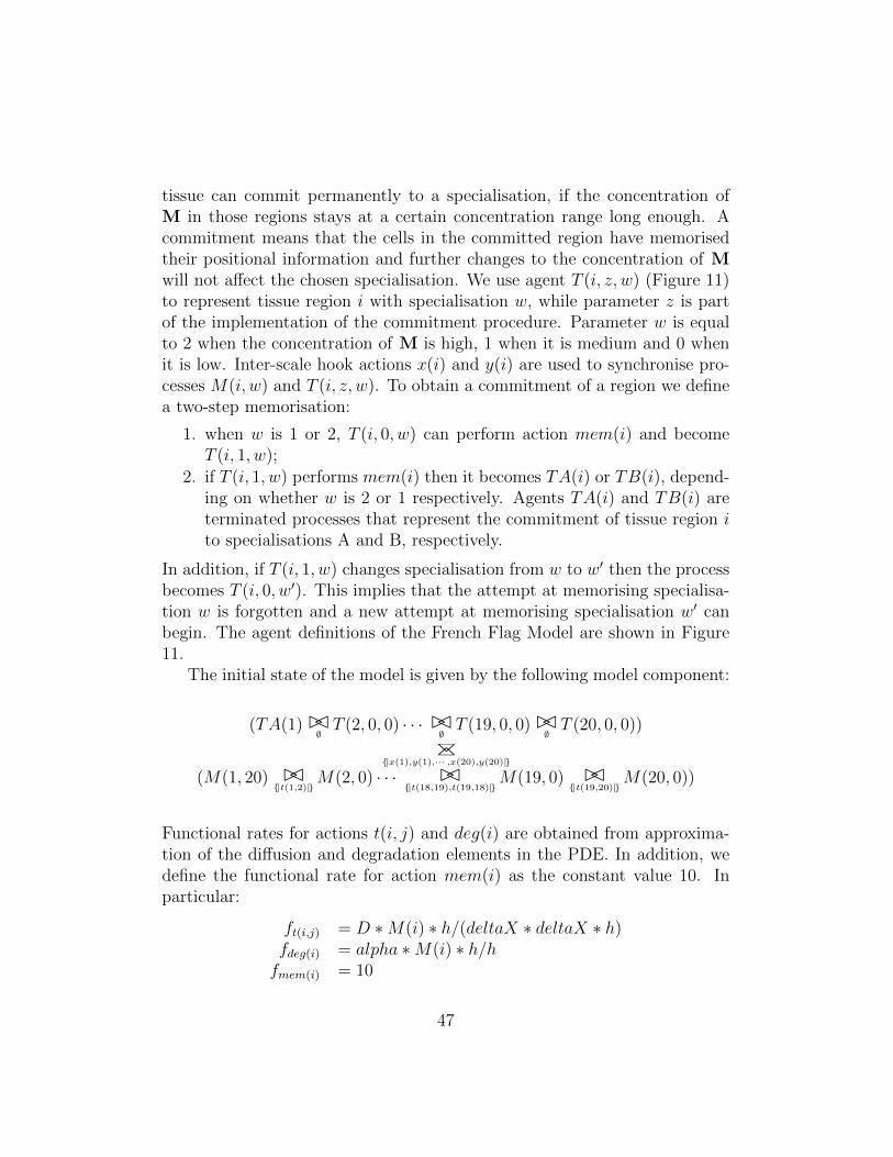
tissue can commit permanently to a specialisation, if the concentration ofM in those regions stays at a certain concentration range long enough. Acommitment means that the cells in the committed region have memorisedtheir positional information and further changes to the concentration of Mwill not affect the chosen specialisation. We use agent T (i, z, w) (Figure 11)to represent tissue region i with specialisation w, while parameter z is partof the implementation of the commitment procedure. Parameter w is equalto 2 when the concentration of M is high, 1 when it is medium and 0 whenit is low. Inter-scale hook actions x(i) and y(i) are used to synchronise pro-cesses M(i, w) and T (i, z, w). To obtain a commitment of a region we definea two-step memorisation:

1. when w is 1 or 2, T (i, 0, w) can perform action mem(i) and becomeT (i, 1, w);

2. if T (i, 1, w) performs mem(i) then it becomes TA(i) or TB(i), depend-ing on whether w is 2 or 1 respectively. Agents TA(i) and TB(i) areterminated processes that represent the commitment of tissue region ito specialisations A and B, respectively.

In addition, if T (i, 1, w) changes specialisation from w to w′ then the processbecomes T (i, 0, w′). This implies that the attempt at memorising specialisa-tion w is forgotten and a new attempt at memorising specialisation w′ canbegin. The agent definitions of the French Flag Model are shown in Figure11.

The initial state of the model is given by the following model component:

(TA(1) BC∅T (2, 0, 0) · · · BC

∅T (19, 0, 0) BC

∅T (20, 0, 0))

BC

{|x(1),y(1),··· ,x(20),y(20)|}

(M(1, 20) BC{|t(1,2)|}

M(2, 0) · · · BC{|t(18,19),t(19,18)|}

M(19, 0) BC{|t(19,20)|}

M(20, 0))

Functional rates for actions t(i, j) and deg(i) are obtained from approxima-tion of the diffusion and degradation elements in the PDE. In addition, wedefine the functional rate for action mem(i) as the constant value 10. Inparticular:

ft(i,j) = D ∗M(i) ∗ h/(deltaX ∗ deltaX ∗ h)fdeg(i) = alpha ∗M(i) ∗ h/hfmem(i) = 10

47

Table 1: In this table we illustrate the commitments of the 20 regions of the French FlagModel over 100 simulations and at different time points. For each region, counts over thesimulations of commitments (A, B or none, i.e. not committed) are given.

Time Comm. 1 2 3 4 5 6 7 8 9 10

0sA 100 0 0 0 0 0 0 0 0 0B 0 0 0 0 0 0 0 0 0 0none 0 100 100 100 100 100 100 100 100 100

1.5sA 100 100 99 98 93 81 66 35 17 8B 0 0 1 2 7 15 17 30 35 51none 0 0 0 0 0 4 17 35 48 41

3sA 100 100 99 98 93 85 81 62 42 12B 0 0 1 2 7 15 17 33 42 72none 0 0 0 0 0 0 2 5 16 16

4.5sA 100 100 99 98 93 85 83 65 47 17B 0 0 1 2 7 15 17 33 46 78none 0 0 0 0 0 0 0 2 7 5

6sA 100 100 99 98 93 85 83 66 53 18B 0 0 1 2 7 15 17 33 46 79none 0 0 0 0 0 0 0 1 1 3

Time Comm. 11 12 13 14 15 16 17 18 19 20

0sA 0 0 0 0 0 0 0 0 0 0B 0 0 0 0 0 0 0 0 0 0none 100 100 100 100 100 100 100 100 100 100

1.5sA 6 1 0 0 0 0 0 0 0 0B 34 38 28 16 10 5 0 0 0 0none 60 61 72 84 90 95 100 100 100 100

3sA 12 3 0 0 0 0 0 0 0 0B 73 76 69 48 28 13 2 2 0 0none 15 21 31 52 72 87 98 98 100 100

4.5sA 13 4 0 0 0 0 0 0 0 0B 82 88 84 67 48 23 8 2 0 0none 5 8 16 33 52 77 92 98 100 100

6sA 14 4 0 0 0 0 0 0 0 0B 83 95 96 79 61 31 12 3 0 0none 3 1 4 21 39 69 88 97 100 100

48

commitments concentrations

0s

6s

6s

6s

position position

Figure 12: Example of simulations of the process algebra with hooks French Flag Model.On the left: commitments of regions to cell specialisations after 6 seconds. On the right:concentration levels after 6 seconds of the same simulation runs. Top row is the initialcondition.

8.1. Analysis

100 simulations were performed on the model, recording the concentrationlevel of M in the three regions, up to 6 seconds. Commitments of regionswas also recorded. Figure 12 illustrates the initial condition and the typicalresults from single simulations at time 6 seconds. Although some variabilitybetween the runs is visible, a pattern of three distinct commitments is alwaysvisible. The images in the figure are constructed from the model componentrepresenting the current state at time 6 seconds. Each picture represents aone-dimensional space divided into 20 regions with source of morphogen Min the left most region. On the left, commitments to cell differentiation areshown: regions committed to A are represented by the colour black, regionscommitted to B by grey, while non-committed regions by white. On the right,the corresponding concentration levels are shown: each concentration level isrepresented by a different shade of grey, from black (maximum concentration)to white (absence of concentration). The top row shows the initial condition

49

Figure 13: Two extensions of the psPAH French Flag Model. In the first extension, top,two species A and B are added. In the second extension, bottom, species C is added.

(time 0s), while the other three rows show three different simulations at time6s.

Additional data is illustrated in Table 1. In this table commitments ofregions are shown. At time 0, only region 1, the source, is committed tospecialisation A, while all the other regions are not committed. As the timeapproaches 6 seconds, we can see the proportion of the 100 simulations inwhich the regions commit to a certain specialisation. For example, regions 2to 5 present a clear preference for specialisation A, while regions 12 and 13have a marked preference for specialisation B. Although some variability ispresent, a change in preference from left to right is evident.

8.2. Example of Use of Congruence

We illustrate now how the concepts of compositionality and congruencein process algebra can be used to reason about the behaviour of the FrenchFlag Model. In particular, we prove two different extensions of the FrenchFlag model to be Markovian (T ,Γ)-bisimilar by extending the equality ofpart of the system to the equality of the whole system. The two extensionsconsist of the addition of biochemical species A and B in the first case andC in the second. These new species do not interact with morphogen M anddo not diffuse, but nevertheless produce their own behaviour becoming partof the system. The two extensions are illustrated in Figure 13.

Consider the following two molecular models:

1. the concentration of two molecules A and B are modelled by agent

50

Figure 14: Rated derivation graphs of model processes A0(n) BC∅

B0(n) and C0(n), withn ∈ R. Parameter n is omitted.

processes representing their concentration as either high or low. SpeciesA and B are produced or degraded independently according to the massaction kinetic law. Process definitions are as follows:

A0(i) , pA(i).A1(i) A1(i) , dA(i).A0(i)

B0(i) , pB(i).B1(i) B1(i) , dB(i).B0(i)

Reactions, functional rates and set of participants are as follows (pa-rameters k = 1 and h = 1):

RpA : → A fpA(i) = k/h ppA(i) = {A(i)}RdA : A→ fdA(i) = k ∗ A(i) ∗ h/h pdA(i) = {A(i)}RpB : → B fpB(i) = k/h ppB(i) = {B(i)}RdB : B→ fdB(i) = k ∗B(i) ∗ h/h pdB(i) = {B(i)}

The rated derivation graph Dr(A0(n) BC∅B0(n)), where n ∈ R, is shown

in Figure 14, on the left.

2. concentration of molecule C is modelled with three agents, represent-ing high, medium and low concentration. Species C inhibits its ownproduction, so the functional rate associated to the production of C isinversely proportional to its concentration. Species C can also degradeaccording to mass action. Process definitions are as follows:

C0(i) , pC(i).C1(i) C1(i) , pC(i).C2(i) + dC(i).C0(i)

C2(i) , dC(i).C1(i)

Reactions, functional rates and set of participants are as follows (pa-rameters k = 1, k′ = 0.5 and h = 1):

RpC : → C fpC(i) = 1/(k′ ∗ h ∗ (1 + C(i) ∗ h)) ppC(i) = {C(i)}RdC : C→ fdC(i) = k ∗ C(i) ∗ h/h pdC(i) = {C(i)}

51

The rated derivation graph Dr(C0(n)), where n ∈ R, is shown in Figure14, on the right.

Notice that for all n ∈ R, A0(n) BC∅B0(n) 'T ,Γ C0(n) for any T such that

T ∩ {|pA, pB, pC, dA, dB, dC|} = ∅ and with the appropriate environmentΓ. In other words, the two psPAH model components are equivalent if weabstract away from the specific actions they can perform, retaining only thetiming and likelihood of those actions. Recall that set T indicates on whichactions rated derivation graphs Dr(A0(n) BC

∅B0(n)) and Dr(C0(n)) should

be compared. Moreover, a suitable environment Γ is a set of parameterswhere constant parameters of the two models are merged without conflict ofnames.

Assume now that the French Flag Model is updated with the additionof chemicals A and B, which do not interact with morphogen M, but thatare nevertheless present in the system. Assume also that we are interestedin comparing the behaviour of the resulting model with the behaviour of theFrench Flag Model updated with the addition of C instead. Without theneed for looking at the actual behaviour of the two new systems, we canprove that their overall behaviour is identical. We prove this simply usingthe fact that A0(n) BC

∅B0(n) and C0(n) are Markovian (T ,Γ)-bisimilar and

the fact that Markovian (T ,Γ)-bisimulation is a congruence (Proposition 40)and it is transitive (Proposition 37).

Because of Proposition 40 we have that:

(A0(1) BC∅B0(1)) BC

∅M(1, 20) 'T ,Γ C0(1) BC

∅M(1, 20) (1)

In the same way we have:

(A0(2) BC∅B0(2)) BC

∅M(2, 0) 'T ,Γ C0(2) BC

∅M(2, 0) (2)

At this point, notice that wheneverX 'T ,Γ Y andW 'T ,Γ Z, thenX BCLW 'T ,Γ

X BCLZ 'T ,Γ Y BC

LZ. By the transitivity of 'T ,Γ (Proposition 37), we have

X BCLW 'T ,Γ Y BC

LZ. Using this result and Equations (1) and (2) we have:

52

(A0(1) BC∅B0(1)) BC

∅M(1, 20) BC

{|t(1,2)|}

(A0(2) BC∅B0(2)) BC

∅M(2, 0)

'T ,ΓC0(1) BC

∅M(1, 20) BC

{|t(1,2)|}

C0(2) BC∅M(2, 0)

Continuing this demonstration with the composition of the processes repre-senting the remaining spatial regions we obtain:

(A0(1) BC∅B0(1)) BC

∅M(1, 20) BC

{|t(1,2)|}

(A0(2) BC∅B0(2)) BC

∅M(2, 0) BC

{|t(2,3),t(3,2)|}

· · · (A0(20) BC∅B0(20)) BC

∅M(20, 0)

'T ,ΓC0(1) BC

∅M(1, 20) BC

{|t(1,2)|}

C0(2) BC∅M(2, 0) BC

{|t(2,3),t(3,2)|}

· · ·C0(20) BC∅M(20, 0)

And finally:

(TA(1) BC∅T (2, 0, 0) · · · BC

∅T (19, 0, 0) BC

∅T (20, 0, 0))

BC

{|x(1),y(1),··· ,x(20),y(20)|}

((A0(1) BC∅B0(1)) BC

∅M(1, 20) BC

{|t(1,2)|}

(A0(2) BC∅B0(2)) BC

∅M(2, 0) BC

{|t(2,3),t(3,2)|}

· · · (A0(20) BC∅B0(20)) BC

∅M(20, 0))

'T ,Γ(TA(1) BC

∅T (2, 0, 0) · · · BC

∅T (19, 0, 0) BC

∅T (20, 0, 0))

BC

{|x(1),y(1),··· ,x(20),y(20)|}

(C0(1) BC∅M(1, 20) BC

{|t(1,2)|}

C0(2) BC∅M(2, 0) BC

{|t(2,3),t(3,2)|}

· · ·C0(20) BC∅M(20, 0))

(3)

Equation (3) finally proves that the addition of molecules A and B andthe addition of molecule C to the French Flag Model have the same effect on

53

its spatio-temporal behaviour. The two extended versions of the French FlagModel are Markovian (T ,Γ)-bisimilar for any action set T as long as T doesnot contain actions of molecules A, B or C and Γ is the union of all constantparameters of the different parts composing the model, without conflicts ofnames. If this is the case we can assert that, for example, the commitment ofthe regions to a specialisation (T = {|mem(1), . . . ,mem(20)|}) happens withthe same timing and with the same probability in both models.

9. Related Work

PAH bears much similarity to other stochastic process algebras, in partic-ular the syntax and horizontal, multi-way synchronisation operator is similarto PEPA [29]. Our introduction of hook actions to represent communicationbetween scales and a vertical operator to represent synchronisation appearsto be novel. We compare our approach with other process algebras that haveprioritised or preemptive actions and the use of probes.

One alternative way to implement hook synchronisation might be to usea process algebra with priority such as EMPA [32]. In this setting, one couldreplace composed actions a[h] with two consecutive actions a and h, whereh has higher priority than a. Actions representing events happening withina scale would have the lowest priority, while higher priority could be usedto represent events happening between scales. There are two disadvantageswith this approach. First, actions with a certain priority would interleavewith actions with different priorities generating additional intermediate statesthat could be avoided a priori using hook synchronisation. Second, whenmultiple high priority actions are available, multiple, non-deterministic pathsof execution are possible. In PAH more control is given to the modellerconcerning how to model the response of a scale to events generating multipleinter-scale effects at the same time. A detailed comparison of PAH with asimple process algebra and a process algebra with priority is given in [2].

Another alternative involves preemptive actions, as provided by the onlyprocess algebra we are aware of that aims specifically to model multi-scalebiological systems in process algebra (PAPC) [26]. PAPC is an extensionof CCS that introduces a distinction between preemptive and conservativeactions and a new summation operation. These extensions allow the rep-resentation of actions that are running and have not yet terminated. Thismeans that a set of actions might be running at the same time and interferewith each other, mimicking interactions between biological scales.

54

The concept of using processes to “observe” actions in a process algebramodel was first introduced in [35] for testing whether a process can performgiven computations, i.e. sequences of actions. In this work an example isgiven in the context of CCS. More recently, a similar approach was intro-duced with Probes [36, 37] in PEPA. In this setting, processes (probes) areconstructed by regular expressions and are used to query a model. Specialstart and stop labels are added to certain actions to indicate entering andleaving states that satisfy the query. Although there are analogies, our ap-proach does not aim to query the system, but to formalise and characterisethe way we can observe its behaviour from different scales. Moreover, regu-lar expressions might in some cases not be powerful enough to construct theprocesses that we need to observe biochemical actions.

Finally, our work bears similarities to logical modelling approaches suchas Rene Thomas framework [38] and the Process Hitting formalism [39]. Inanalogy with our framework, in these approaches a fixed number of variablesis modelled by a finite number of levels. Additionally, a threshold systemis used to determine the nature of the interactions between variables, suchas activator or inhibitor, while we use thresholds to determine interactionsbetween biological scales.

10. Conclusions

PAH has been designed for multi-scale modelling of biological systems,using processes to represent biological scales, actions to represent biologicalevents and functional rates to determine the timing of events. The introduc-tion of composed actions and vertical synchronisation allows for the explicitrepresentation of scales and interactions within and between scales. More-over, features such as composition and relation of PAH processes are particu-larly amenable to the multi-scale modelling of biological systems, where theycan be used to manipulate different scales in the same formal framework.

We introduced PAH through a series of examples, then we proceeded tothe definition of the syntax and semantics of PAH, before providing defi-nitions of compatibility L-bisimulation and Markovian (T ,Γ)-bisimulationbetween PAH processes. We illustrated how the former relation can be usedto aid model development for a model of tissue growth by checking that twoscales have been defined correctly and can interact as intended by the mod-eller. We demonstrated how the latter can be used for reasoning about aknown biological example: the french flag problem. In this system a group

55

of identical cells in a tissue are differentiated into subgroups according tothe diffusion of a morphogen from a source. Differentiation depends uponthe concentration in various regions and the standard model is a PDE. Here,we showed how to represent the problem in PAH, discretising both concen-trations and spatial regions. We gave simulation analysis results computedusing our bespoke interpreter. We then considered two possible extensions tothe model: the addition of species A and B that are produced and degradedindependently of the rest of the system, and the addition of species C that isalso independent of the rest of the system and inhibits its own production.We used our Markovian (T ,Γ)-bisimulation to show that the two additionshave the same behaviour, thus demonstrating an advantage of an algebraicframework over (partial) differential equations. Finally, we compared ourapproach with alternatives based on prioritised or preemptive events.

10.1. Future Work

Possible extensions of PAH include:

• implementation of compatibility L-bisimulation checker. In Section 5,we have defined a relation between PAH processes. In order to usethis in practice we need to define and implement an algorithm to checkwhether this relation holds for any pair of given processes. A possibledirection is to follow an approach analogous to the algorithm for weakbisimulation discussed in [40];

• approximate equivalence relations. Markovian (T ,Γ)-bisimulation is afundamental equivalence relations for PAH. However, biological appli-cations require a more qualitative interpretation of behaviour, wheretwo systems can be considered similar, though not identical. Approxi-mate equivalence relations and distance measures between models [41]may prove an interesting direction to explore. If we associate locationswith explicit coordinates and compute distances between processes inspace, these metrics could be useful in the computation of approximateequivalence relations;

• efficient stochastic simulations. At the moment, the simulator thatsamples trajectories of transitions is not optimised. At each step thecomplete set of rated transitions is computed, while it could be thecase that only a few processes are affected by the last step and thatonly a few transitions need to be updated. Improvements will depend

56

upon determining which processes are affected by a transition. Withthis information, known improvements to stochastic simulations of bio-chemical reactions and their diffusion, e.g. [42, 43], can be adapted andintegrated in our approach;

• Development of a high level representation for non-experts. The pro-cess algebra framework may be difficult to use by non-experts. Animportant step toward the dissemination of our work in the systemsbiology community is the development of a higher level language or agraphical representation that would make this work more accessible tonon-experts.

11. Acknowledgements

This research was supported by a Lord Kelvin/ Adam Smith Scholarshipof the University of Glasgow and by the EPSRC funded SIGNAL project(http://www.signalproject.org.uk/).

References

[1] A. Degasperi, M. Calder, Multi-scale modelling of biological systemsin process algebra with multi-way synchronisation, in: Proceedings ofCMSB 2011, ACM Press, 2011, pp. 195–208.

[2] A. Degasperi, Multi-Scale Modelling of Biological Systems in ProcessAlgebra, Ph.D. thesis, University of Glasgow, 2011.

[3] H. Kitano, Systems Biology: A Brief Overview, Science 295 (2002)1662–1664.

[4] E. Klipp, R. Herwig, A. Kowald, C. Wierling, H. Lehrach, SystemsBiology in practice, Wiley-Vch, 2005.

[5] H. Meinhardt, Models of biological pattern formation: from elementarysteps to the organization of embryonic axes, Curr. Top. Dev. Biol. 81(2008) 1–63.

[6] G. B. Ermentrout, L. E. Keshet, Cellular Automata Approaches toBiological Modelling, Journal of Theoretical Biology 160 (1993) 97–133.

57

[7] M. Hucka, A. Finney, H. M. Sauro, H. Bolouri, J. C. Doyle, H. Kitano,The systems biology markup language (SBML): a medium for represen-tation and exchange of biochemical network models, Bioinformatics 19(2003) 524–531.

[8] H. Kitano, A graphical notation for biochemical networks, BIOSILICO1 (2003) 169–176.

[9] M. Calder, S. Gilmore, J. Hillston, Modelling the influence of RKIP onthe ERK signalling pathway using the stochastic process algebra PEPA,LNCS Trans. on Computat. Syst. Biol. VII 4230 (2006) 1–23.

[10] C. Priami, P. Quaglia, Beta-binders for biological interactions, in: Lec-ture Notes in Computer Science, volume 3082, Springer Verlag, 2005,pp. 20–33.

[11] F. Ciocchetta, J. Hillston, Bio-PEPA: A framework for the modellingand analysis of biological systems, Theoretical Computer Science 410(2009) 3065–3084.

[12] L. Bortolussi, A. Policriti, Modeling biological systems in stochasticconcurrent constraint programming, Constraints 13 (2008) 66–90.

[13] V. Danos, J. Feret, W. Fontana, R. Harmer, J. Krivine, Rule-basedmodelling of cellular signalling, in: Lecture Notes in Computer Science,Springer Verlag, 2007, pp. 17–41.

[14] M. L. Blinov, J. R. Faeder, B. Goldstein, W. S. Hlavacek, BioNetGen:software for rule-based modeling of signal transduction based on theinteractions of molecular domains, Bioinformatics 20 (2004) 3289–3291.

[15] L. Calzone, F. Fages, S. Soliman, Biocham: An environment for mod-elling biological systems and formalizing experimental knowledge, Bioin-formatics 22 (2006) 1805–1807.

[16] M. Pedersen, G. Plotkin, A language for biochemical systems, in: Lec-ture Notes in Bioinformatics, volume 5307, Springer Verlag, 2008, pp.63–82.

[17] R. Milner, Communication and Concurrency, Prentice-Hall, Inc., 1989.

58

[18] C. A. R. Hoare, Communicating Sequential Processes, Prentice-Hall,Inc., 1985.

[19] A. Regev, W. Silverman, E. Shapiro, Representation and simulationof biochemical processes using the pi-calculus process algebra, PacificSymposium on Biocomputing (2001) 459–470.

[20] C. Priami, A. Regev, E. Shapiro, W. Silverman, Application of astochastic name-passing calculus to representation and simulation ofmolecular processes, Inf. Process. Lett. 80 (2001) 25–31.

[21] L. Cardelli, Brane calculi, in: Lecture Notes in Bioinformatics, volume3082, Springer Verlag, 2005, pp. 257–278.

[22] J. O. Dada, P. Mendes, Multi-scale modelling and simulation in systemsbiology, Integrative Biology 3 (2011) 86–96.

[23] D. C. Walker, J. Southgate, The virtual cell–a candidate co-ordinator for’middle-out’ modelling of biological systems, Briefings in Bioinformatics10 (2009) 450–461.

[24] D. C. Walker, N. T. Georgopoulos, J. Southgate, From pathway topopulation - a multiscale model of juxtacrine egfr-mapk signalling, BMCSystems Biology 2 (2008) 102.

[25] D. Noble, The Music of Life: Biology Beyond the Genome, Oxford Uni-versity Press, 2006.

[26] R. Barbuti, G. Caravagna, A. Maggiolo-Schettini, P. Milazzo, S. Tini,Foundational aspects of multiscale modeling of biological systems withprocess algebras, Theoretical Computer Science 431 (2012) 96–116.

[27] C. Athale, Y. Mansury, T. S. Deisboeck, Simulating the impact ofa molecular ‘decision-process’ on cellular phenotype and multicellularpatterns in brain tumors, Journal of Theoretical Biology 233 (2005)469–481.

[28] Z. Wang, L. Zhang, J. Sagotsky, T. S. Deisboeck, Simulating non-small cell lung cancer with a multiscale agent-based model, Journal ofTheoretical Biology 233 (2005) 469–481.

59

[29] J. Hillston, A Compositional Approach to Performance Modelling, Cam-bridge University Press, 1996.

[30] F. Ciocchetta, A. Degasperi, J. Hillston, M. Calder, Some investigationsconcerning the CTMC and the ODE model derived from Bio-PEPA, in:Electronic Notes in Theoretical Computer Science, volume 229, Elsevier,2009, pp. 145–163.

[31] A. Degasperi, M. Calder, Process algebra with hooks for models ofpattern formation, in: CS2Bio 2010, Electronic Notes in TheoreticalComputer Science, volume 268, Elsevier, 2010, pp. 31–47.

[32] M. Bernardo, R. Gorrieri, Extended Markovian Process Algebra, in:Lecture Notes in Computer Science, volume 1119, Springer Verlag, 1996,pp. 315–330.

[33] L. Wolpert, The French flag problem: A Contribution to the Discussionon Pattern Formation and Regulation, Towards a Theoretical Biology1 (1968) 125–133.

[34] U. Alon, An Introduction to Systems Biology, Chapman & Hall/CRC,2006.

[35] R. D. Nicola, M. C. B. Hennessy, Testing equivalences for processes,Theoretical Computer Science (1984) 83–133.

[36] A. Argent-Katwala, J. T. Bradley, N. J. Dingle, Expressing performancerequirements using regular expressions to specify stochastic probes overprocess algebra models, in: Fourth International Workshop on Softwareand Performance, ACM Press, 2004, pp. 49–58.

[37] A. Clark, S. Gilmore, State-aware performance analysis with eXtendedstochastic probes, in: Lecture Notes in Computer Science, volume 5261,Springer Verlag, 2008, pp. 125–140.

[38] R. Thomas, M. Kaufman, Multistationarity, the basis of cell differenti-ation and memory. ii. logical analysis of regulatory networks in terms offeedback circuits, Chaos 11 (2001) 180–195.

[39] L. Pauleve, O. R. M. Magnin, Refining dynamics of gene regulatorynetworks in a stochastic p-calculus framework, T. Comp. Sys. Biology13 (2011) 171–191.

60

[40] H. Hermanns, M. Siegle, Bisimulation Algorithms for Stochastic ProcessAlgebras and their BDD-based Implementation, in: Lecture Notes inComputer Science, volume 1601, Springer Verlag, 1999, pp. 244–264.

[41] S. Tini, Non-expansive epsilon-bisimulations for probabilistic processes,Theoretical Computer Science 411 (2010) 2202–2222.

[42] J. Elf, M. Ehrenberg, Spontaneous separation of bi-stable biochemicalsystems into spatial domains of opposite phases, Systems Biology 1(2004) 230–236.

[43] M. A. Gibson, J. Bruck, Efficient exact stochastic simulation of chemicalsystems with many species and many channels, The Journal of PhysicalChemistry A 104 (2000) 1876–1889.

Appendix A. Multi-Sets

We use {| and |} to delimit a multi-set. For example, A = {|5, 6, 6, 7, 7, 7|}is a multi-set.

We define a multi-set M as the pair (M ′,mM), where M ′ is a set contain-ing the same elements of M with no repetitions and mM is the associatedmultiplicity function, such that for all x ∈M ′, mM(x) is equal to the numberof times x appears in M . For all x ∈ M ′, mM(x) is equal to zero if x doesnot appear in M . For example, multi-set A is defined as the pair (A′,mA),where A′ ⊂ N, A′ = {5, 6, 7}, and mA : N→ N, mA(5) = 1, mA(6) = 2 andmA(7) = 3.

Given two multi-sets A and B, defined as (A′,mA) and (B′,mB), thefollowing operations are defined:

• multi-set union: A ∪ B = (A′ ∪ B′,mA∪B), where for all x ∈ A′ ∪ B′,mA∪B(x) = max(mA(x),mB(x));

• multi-set sum: A ] B = (A′ ∪ B′,mA]B), where for all x ∈ A′ ∪ B′,mA]B(x) = mA(x) +mB(x);

• multi-set intersection: A∩B = (A′∩B′,mA∩B), where for all x ∈ A′∩B′,mA∩B(x) = min(mA(x),mB(x));

• multi-set difference: A\B = (A′,mA\B), where for all x ∈ A′, mA\B(x) =min(0,mA(x)−mB(x)).

61

Moreover we define:

• A ⊆ B ⇔ for all x ∈ A′ ∪B′, mA(x) ≤ mB(x);

• |A| =∑x∈A′

mA(x).

Appendix B. Proofs

Proof of Proposition 40. Proof of each case:

1. We know by assumption that P1 'T ,Γ P2. This implies P1, P2 ∈ C,with C ∈ Pm/ 'T ,Γ. Now, FiltMoves(A[E ].P1)T = {|(((A\T ), E), P1)|}and FiltMoves(A[E ].P2)T = {|(((A \ T ), E), P2)|}. This implies ∀C ∈Pm/ 'T ,Γ

FiltCompAct(A[E ].P1, C)T = FiltCompAct(A[E ].P2, C)T

2. P1 + Q and P2 + Q are definition processes. Because P1 'T ,Γ P2 wehave that ∀C ∈ Pm/ 'T ,Γ

FiltCompAct(P1 +Q, C)T =FiltCompAct(P1, C)T ] FiltCompAct(Q, C)T =FiltCompAct(P2, C)T ] FiltCompAct(Q, C)T =

FiltCompAct(P2 +Q, C)T

3. We prove that the relation R = {(P1 BCL Q,P2 BCL Q) | P1 'T ,Γ P2} isa Markovian (T ,Γ)-bisimulation. We consider four cases:

(a) ∀r ∈ R, (A, E , r) 6∈ FiltAct(P1 BCL Q)T ,Γ. This implies that ∀r ∈R, (A, E , r) 6∈ FiltAct(P2 BCL Q)T ,Γ, because a filtered activity for

P BCLQ is either a filtered activity of P , a filtered activity of Q or

it is derived from a closed activity which is the synchronisation ofan open activity from P and one from Q and P1 'T ,Γ P2 implies

• ∀r ∈ R, (A, E , r) 6∈ FiltAct(P1)T ,Γ ⇔ ∀r ∈ R, (A, E , r) 6∈FiltAct(P2)T ,Γ;

• ∀C ∈ Pm/ 'T ,Γ OpenAct(P1, C) = OpenAct(P2, C).It follows that ∀C ∈ Pm/ 'T ,Γ

νT ,Γ(P1 BCL Q,A, E , C) = νT ,Γ(P2 BCL Q,A, E , C) = 0

62

(b) ∃r ∈ R, ((A, E , r), P ′1 BCL Q) ∈ FiltMoves(P1 BCL Q)T ,Γ. Recallthat P1 'T ,Γ P2 implies

∃r ∈ R, ((A, E , r), P ′1) ∈ FiltMoves(P1)T ,Γ ⇔∃r′ ∈ R, ((A, E , r′), P ′2) ∈ FiltMoves(P2)T ,Γ

with P ′1 'T ,Γ P ′2, because νT ,Γ(P1,A, E , [P ′1]'T ,Γ) = νT ,Γ(P2,A, E , [P ′1]'T ,Γ

).It follows that

νT ,Γ(P1 BCL Q,A, E , [P ′1 BCL Q]R) = νT ,Γ(P1,A, E , [P ′1]'T ,Γ) =

νT ,Γ(P2,A, E , [P ′1]'T ,Γ) = νT ,Γ(P2 BCL Q,A, E , [P ′2 BCL Q]R)

It is also important to recall that if an activity is filtered thenit is derived from a closed activity, which in turn means that nofurther synchronisation is possible via BC

L. This is ensured by

Proposition 14 and Definition 15.(c) ∃r ∈ R, ((A, E , r), P1 BCL Q′) ∈ FiltMoves(P1 BCL Q)T ,Γ. It fol-

lows that

νT ,Γ(P1 BCL Q,A, E , [P1 BCL Q′]R) = νT ,Γ(Q,A, E , [Q′]'T ,Γ) =

= νT ,Γ(P2 BCL Q,A, E , [P1 BCL Q′]R)

Because P1 'T ,Γ P2 and so P2 BCL Q′ ∈ [P1 BCL Q′]R.(d) ∃r ∈ R, ((A, E , r), P ′1 BCL Q′) ∈ FiltMoves(P1 BCL Q)T ,Γ. The fil-

tered move ((A, E , r), P ′1 BCL Q′) must be the result of a synchro-nisation between an open move from P1 and an open move from Q.In particular, it must be that ∃(A1[E1],∆1) ∈ OpenAct(P1, [P

′1]'T ,Γ

)and ∃(A2[E2],∆2) ∈ OpenAct(Q, [Q′]'T ,Γ

) such that:

• B = A1 ∪ A2, E = E1 ] E2 and ∆ = ∆1 ∪∆2;

• (B[E ],∆) ∈ ClosedAct(P1 BCL Q);

• b ∈ B and fb ∈ F and Γ ∪∆ ` fb → k and A = B ∩ T ;

• r = k/π(ClosedAct(P1 BCL Q), b).

Moreover, from P1 'T ,Γ P2 we have that

((A1[E1],∆1), P ′1) ∈ OpenMoves(P1)⇔((A1[E1],∆1), P ′2) ∈ OpenMoves(P2)

with P ′1 'T ,Γ P ′2, becauseOpenAct(P1, [P′1]'T ,Γ

) = OpenAct(P2, [P′1]'T ,Γ

).It follows that

νT ,Γ(P1 BCL Q,A, E , [P ′1 BCL Q′]R) = νT ,Γ(P2 BCL Q,A, E , [P ′1 BCL Q′]R)

where P ′2 BCL Q′ ∈ [P ′1 BCL Q′]R.

63

4. We prove that the relation R = {(P1 BC

LQ,P2 BC

LQ) | P1 'T ,Γ P2} is a

Markovian (T ,Γ)-bisimulation. We consider four cases:

(a) ∀r ∈ R, (A, E , r) 6∈ FiltAct(P1 BC

LQ)T ,Γ. This implies that ∀r ∈

R, (A, E , r) 6∈ FiltAct(P2 BC

LQ)T ,Γ, because a filtered activity for

P BCLQ is either a filtered activity of P , a filtered activity of Q or

it is derived from a synchronisation of a filtered activity from Pand an open activity from Q or a filtered activity from Q and anopen activity from P and P1 'T ,Γ P2 implies

• ∀r ∈ R, (A, E , r) 6∈ FiltAct(P1)T ,Γ ⇔ ∀r ∈ R, (A, E , r) 6∈FiltAct(P2)T ,Γ;

• ∀C ∈ Pm/ 'T ,Γ OpenAct(P1, C) = OpenAct(P2, C).It follows that ∀C ∈ Pm/ 'T ,Γ

νT ,Γ(P1 BC

LQ,A, E , C) = νT ,Γ(P2 BC

LQ,A, E , C) = 0

(b) ∃r ∈ R, ((A, E , r), P ′1 BC

LQ) ∈ FiltMoves(P1 BC

LQ)T ,Γ. This im-

plies that ((A, E , r), P ′1) ∈ FiltMoves(P1)T ,Γ and that E ∩ L = ∅.Moreover,

∃r ∈ R, ((A, E , r), P ′1) ∈ FiltMoves(P1)T ,Γ ⇔∃r′ ∈ R, ((A, E , r′), P ′2) ∈ FiltMoves(P2)T ,Γ

with P ′1 'T ,Γ P ′2, because νT ,Γ(P1,A, E , [P ′1]'T ,Γ) = νT ,Γ(P2,A, E , [P ′1]'T ,Γ

).It follows that

νT ,Γ(P1 BC

LQ,A, E , [P ′1 BC

LQ]R) = νT ,Γ(P1,A, E , [P ′1]'T ,Γ

) =

νT ,Γ(P2,A, E , [P ′1]'T ,Γ) = νT ,Γ(P2 BC

LQ,A, E , [P ′1 BC

LQ]R)

(c) ∃r ∈ R, ((A, E , r), P1 BC

LQ′) ∈ FiltMoves(P1 BC

LQ)T ,Γ. This im-

plies that ((A, E , r), Q′) ∈ FiltMoves(Q)T ,Γ and that E ∩ L = ∅.Because ∀C ∈ Pm/ 'T ,Γ, OpenAct(P1, C) = OpenAct(P2, C) then

νT ,Γ(P1 BC

LQ,A, E , [P1 BC

LQ′]R) = νT ,Γ(Q,A, E , [Q′]'T ,Γ

) =

νT ,Γ(P2 BC

LQ,A, E , [P1 BC

LQ′]R)

(d) ∃r ∈ R, ((A, E , r), P ′1 BC

LQ′) ∈ FiltMoves(P1 BC

LQ)T ,Γ. This im-

plies that filtered move ((A, E , r), P ′1 BC

LQ′) is the result of the

64

synchronisation of a filtered move of P1 and an open move of Q orthe synchronisation of a filtered move from Q and an open movefrom P1.In this case we have

νT ,Γ(P1 BC

LQ,A, E , [P ′1 BC

LQ′]R) =∑

i∈I

νT ,Γ(P1,Ai, Ei, [P ′1]'T ,Γ) +

∑j∈J

νT ,Γ(Q,Aj, Ej, [Q′]'T ,Γ) =∑

i∈I

νT ,Γ(P2,Ai, Ei, [P ′1]'T ,Γ) +

∑j∈J

νT ,Γ(Q,Aj, Ej, [Q′]'T ,Γ) =

νT ,Γ(P2 BCLQ,A, E , [P ′1 BC

LQ′]R)

Once again because

∃r ∈ R, ((A, E , r), P ′1) ∈ FiltMoves(P1)T ,Γ ⇔∃r′ ∈ R, ((A, E , r′), P ′2) ∈ FiltMoves(P2)T ,Γ

with P ′1 'T ,Γ P ′2, because νT ,Γ(P1,A, E , [P ′1]'T ,Γ) = νT ,Γ(P2,A, E , [P ′1]'T ,Γ

).Moreover

• i ∈ I if and only if ∃B,F ,∆, Q′ s.t. ((B[F ],∆), Q′) ∈Moves(Q)and B ⊆ Ei ∩ L and A = Ai ∪ (B ∩ T ) and E = (Ei \ B) ] Fand ¬(∃B′,F ′,∆′, Q′′ s.t. ((B′[F ′],∆′), Q′′) ∈ Moves(Q) andB′ ⊆ Ei ∩ L and |B′| > |B|);• j ∈ J if and only if ∃B,F ,∆, P ′1 s.t. ((B[F ],∆), P ′1) ∈Moves(P )

and B ⊆ Ej ∩ L and A = Aj ∪ (B ∩ T ) and E = (Ej \ B) ] Fand ¬(∃B′,F ′,∆′, Q′′ s.t. ((B′[F ′],∆′), P ′′1 ) ∈Moves(P1) andB′ ⊆ Ej ∩ L and |B′| > |B|).

We also use the fact that ∀C ∈ Pm/ 'T ,Γ, OpenAct(P1, C) =OpenAct(P2, C).

Since we proved all four cases, the result holds.

65