A Programming Approach to Estimate Production Functions using

Bounds on the True Production Set

January 29, 1997

David K. Lambert

Discussion Paper APES97-01

Department of Applied Economics and StatisticsUniversity of Nevada, Reno, NV 89557-0105 USA

davel@unr.edu

The author retains all rights to the material included in this paper. Electronic and printeddissemination of the paper is allowed subject to acknowledgment of the authorship andsource of the manuscript.

________________________________________________________________________

Abstract

Varian (1984) developed procedures to establish bounds on a true convex negative

monotonic production set that p-rationalizes a set of data consistent with the weak axiom

of profit maximization. These bounds can provide additional information for estimating

parametric production functions. A mathematical programming procedure is developed to

maximize various measures of goodness of fit of alternative parametric specifications

relative to the true production set.

Key words: Nonparametric techniques; Production; Production functions

JEL classification: C14, C61, D24

2

A Programming Approach to Estimate Production Functions using Bounds on

the True Production Set

1. Introduction

Characterization of technology generally results from econometric estimation of a

primal or dual system of equations representing optimal production choices under

changing economic conditions. For example, one might assume profit maximizing

behavior with output choices endogenous to the firm. A profit function is specified, factor

demand and output supply functions are then derived and estimated, and statistical tests of

the properties of the underlying technology are conducted.

Several problems may arise from the conventional approach. First, a limited

number of observations may be available. For example, degree of freedom problems may

require a priori restrictions on the structure of technology, consequently limiting the set of

regularity tests that can be performed. Second, the results of hypothesis testing may in

large part hinge upon the form of the functional relationship chosen by the analyst. The

maintained hypothesis of the functional form itself cannot be directly tested (Varian,

1984). Although different specifications may fit the data fairly well, predicted behavioral

responses may differ significantly depending upon functional form (Shumway and Lim,

1993). Finally, there may be no need to rely upon a parametric specification. Varian

(1984, 1990) has demonstrated that complex models of optimizing behavior can be tested

using nonparametric procedures. Nonparametric tests allow a separation of the joint

hypotheses of optimizing behavior and functional specification.

3

There are advantages to a parametric representation of technology, however. For

example, a continuous production function permits numerical estimates of comparative

statics and characterization of technical change. Nonparametric techniques have met with

some success in these areas (Chavas and Cox, 1992; Fare&& and Grosskopf, 1985).

However, the piece-wise representation of the production surface resulting from the linear

programming models underlying the approach may limit the usefulness of nonparametric

estimates (Lambert, 1996).

The objective of the present research is to combine nonparametric tests of

optimizing behavior with subsequent estimation of a parametric production function. The

results of the nonparametric tests will suggest both functional specification and

appropriate parameter restrictions. The design matrix for the estimation of the production

function is constructed using procedures attributed to Afriat (1972), Hanoch and

Rothschild (1972), and Varian (1984). A large number of production sets are generated

that are known to bound a true production set. These upper and lower bounds then form

the right hand side values in a set of inequality constraints defining the feasible region for

two related mathematical programming problems. Parameter estimates result from two

different mathematical programming problems: (1) maximizing the goodness of fit of

estimated production functions to the output set known to bound the true output level,

and (2) maximizing the number of predicted levels of output that fall within the bounds on

the true production set. The approach follows Hanoch and Rothschild’s (1972, page 257)

suggestion that researchers test the nature of technology using nonparametric tests before

estimating specific cost or production functions.

4

The paper is organized as follows. The following section relies upon Varian’s

(1984) derivation of bounds on the true production set given observations that are

consistent with the weak axiom of profit maximization. The third section develops

mathematical programming procedures to estimate parametric summary functions given

the bounds on the true production set. Nonparametric testing procedures are presented in

the fourth section that are used for specification testing. The final sections present an

application of the procedures to aggregate U.S. agricultural production over the period

1948-1983.

2. The Nature of Technology

Consider a technology that transforms inputs x = {x1, x2, ..., xn} into outputs, y =

{y 1, y2, ..., ym}. Define the production set as :

Y = ( ){ }y, x x y x y+n

+m: , ,∈ ℜ ∈ ℜ can produce (1)

Varian places minimal restrictions on the production set. Namely, Y is negative

monotonic if (y, x) is in Y and (y′, -x′) < (y, -x) implies that (y′, x′) is in Y.

Further restrictions on Y arise as one assumes optimizing behavior. For our

purposes, we restrict our consideration to characteristics of Y that are consistent with

profit maximization. Our intent is to characterize a production set that p-rationalizes the

data, where “p” represents “profit” (Varian, 1984). If we have t observations on prices

and quantities, (pi, yi, ri, xi), i = 1,..., t, a production set Y p-rationalizes the data if piy -

rix < piyi - rixi for all (y, x) in Y. In this case, the set of observations is consistent with

5

the weak axiom of profit maximization (WAPM) (Varian, 1984). In words, no feasible

draw from production set Y could have resulted in greater profits than were actually

observed under conditions (pi, ri). For the remainder of the discussion, we consider a

single measure of output, y. This allows us to establish the link between observed

behavior and production theory by relying on Varian’s theorem 4:

Theorem 4 (Varian, 1984, page 584): The following conditions are equivalent: (1) There

exists a production function that p-rationalizes the data. (2) y j < yi + (wi/pi)(x j-xi) for all

i and j. (3) There exists a continuous, concave, monotonic production function that

p-rationalizes the data.

Awareness of the existence of a production function does not lead directly to its

specification. A candidate production function that p-rationalizes the data may not be

unique. Instead, an entire class of functions may be consistent with the observed behavior

(Chavas and Cox, 1995). This class of functions can, however, be bounded by two

particular specifications of the production function, the inner bound YI and the outer

bound YO (Varian, 1984).

The inner bound on the true production set is defined (Varian, 1984):

YI = com-{y, x}, (2)

where com-{y, x} is the negative convex monotonic hull defined over observed vectors

(yi, xi). Pertinent aspects of Varian’s theorem 14 (Varian, 1984, page 594) are that, if Y is

a convex negative monotonic production set that p-rationalizes the data, then Y ⊃ YI, and

if Z is a convex negative monotonic production set strictly contained in YI, then Z cannot

6

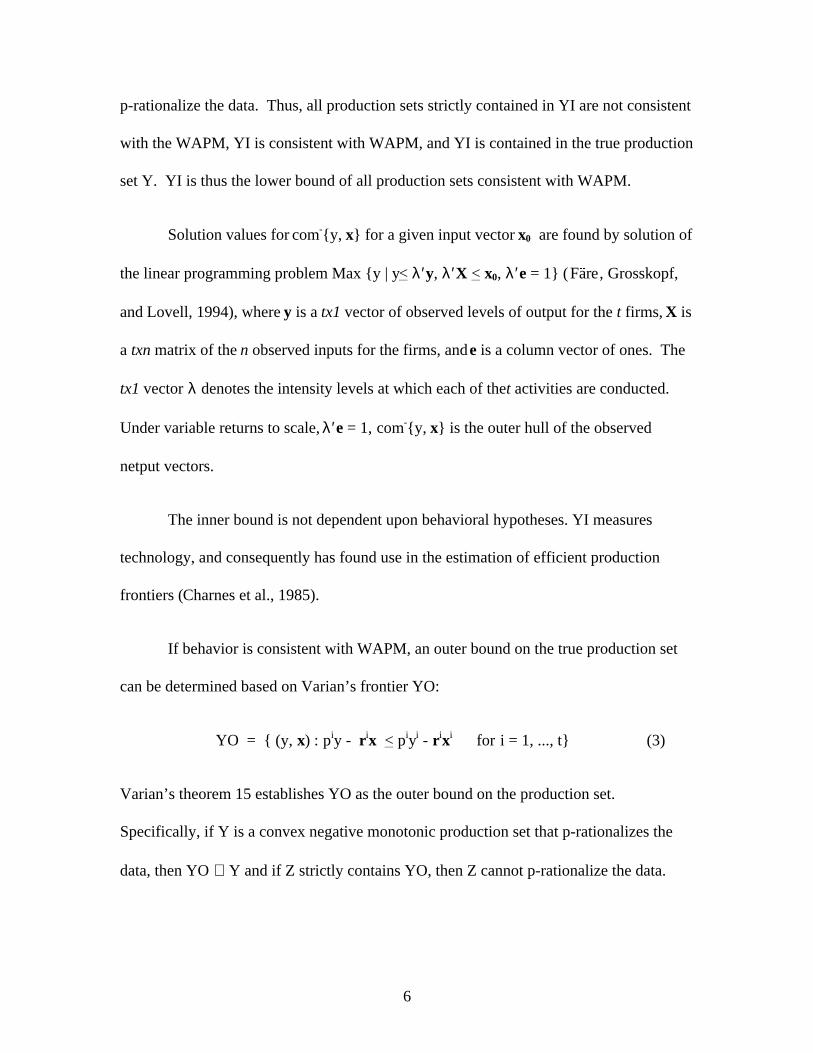
p-rationalize the data. Thus, all production sets strictly contained in YI are not consistent

with the WAPM, YI is consistent with WAPM, and YI is contained in the true production

set Y. YI is thus the lower bound of all production sets consistent with WAPM.

Solution values for com-{y, x} for a given input vector x0 are found by solution of

the linear programming problem Max {y | y < λ′y, λ′X < x0, λ′e = 1} (Fare&& , Grosskopf,

and Lovell, 1994), where y is a tx1 vector of observed levels of output for the t firms, X is

a txn matrix of the n observed inputs for the firms, and e is a column vector of ones. The

tx1 vector λ denotes the intensity levels at which each of the t activities are conducted.

Under variable returns to scale, λ′e = 1, com-{y, x} is the outer hull of the observed

netput vectors.

The inner bound is not dependent upon behavioral hypotheses. YI measures

technology, and consequently has found use in the estimation of efficient production

frontiers (Charnes et al., 1985).

If behavior is consistent with WAPM, an outer bound on the true production set

can be determined based on Varian’s frontier YO:

YO = { (y, x) : piy - rix < piyi - rixi for i = 1, ..., t} (3)

Varian’s theorem 15 establishes YO as the outer bound on the production set.

Specifically, if Y is a convex negative monotonic production set that p-rationalizes the

data, then YO ⊃ Y and if Z strictly contains YO, then Z cannot p-rationalize the data.

7

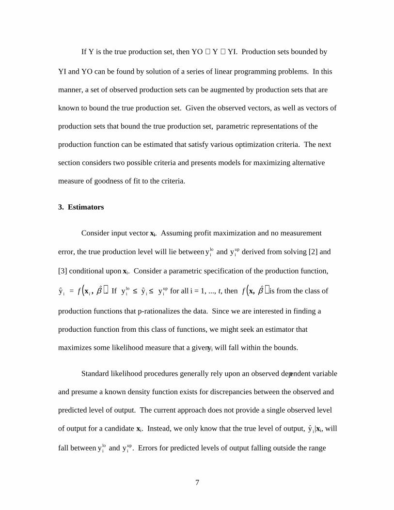
If Y is the true production set, then YO ⊃ Y ⊃ YI. Production sets bounded by

YI and YO can be found by solution of a series of linear programming problems. In this

manner, a set of observed production sets can be augmented by production sets that are

known to bound the true production set. Given the observed vectors, as well as vectors of

production sets that bound the true production set, parametric representations of the

production function can be estimated that satisfy various optimization criteria. The next

section considers two possible criteria and presents models for maximizing alternative

measure of goodness of fit to the criteria.

3. Estimators

Consider input vector xi. Assuming profit maximization and no measurement

error, the true production level will lie between yilo and yi

up derived from solving [2] and

[3] conditional upon xi. Consider a parametric specification of the production function,

( )$

$y = i f ix , β . If yilo ≤ ≤ y i$ yi

up for all i = 1, ..., t, then ( ) f x, $β is from the class of

production functions that p-rationalizes the data. Since we are interested in finding a

production function from this class of functions, we might seek an estimator that

maximizes some likelihood measure that a given yi will fall within the bounds.

Standard likelihood procedures generally rely upon an observed dependent variable

and presume a known density function exists for discrepancies between the observed and

predicted level of output. The current approach does not provide a single observed level

of output for a candidate xi. Instead, we only know that the true level of output, $yi |xi, will

fall between yilo and yi

up. Errors for predicted levels of output falling outside the range

8

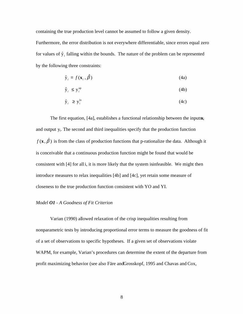
containing the true production level cannot be assumed to follow a given density.

Furthermore, the error distribution is not everywhere differentiable, since errors equal zero

for values of $yi falling within the bounds. The nature of the problem can be represented

by the following three constraints:

$ ( , $)y i if= x β (4a)

$y i ≤ yiup (4b)

$y i ≥ yilo (4c)

The first equation, [4a], establishes a functional relationship between the inputs xi

and output yi. The second and third inequalities specify that the production function

f ( , $)x β is from the class of production functions that p-rationalize the data. Although it

is conceivable that a continuous production function might be found that would be

consistent with [4] for all i, it is more likely that the system is infeasible. We might then

introduce measures to relax inequalities [4b] and [4c], yet retain some measure of

closeness to the true production function consistent with YO and YI.

Model O1 - A Goodness of Fit Criterion

Varian (1990) allowed relaxation of the crisp inequalities resulting from

nonparametric tests by introducing proportional error terms to measure the goodness of fit

of a set of observations to specific hypotheses. If a given set of observations violate

WAPM, for example, Varian’s procedures can determine the extent of the departure from

profit maximizing behavior (see also Färe and Grosskopf, 1995 and Chavas and Cox,

9

1990). If the violations are “small enough,”1 we might then presume that the firm has

made optimal, or at least nearly optimal, choices. Model O1 uses a goodness of fit

measure similar to Varian’s to maximize the goodness of fit of a particular production

function to the true production function bounded by YO and YI.

The estimating model is:

O1. Minimize i=1

φ i

t∑

subject to

$ ( , $)y i if= x β (5a)

( )$y i i≤ +1 φ yiup (5b)

( )$y i i≥ −1 φ yilo (5c)

φ i > 0, $y > 0, and $β unrestricted in sign.2

If $y i lies between the bounds, φ i will equal 0. If $y i is outside of the bounds, φ i will be

greater than 0, and will represent the minimum proportional expansion (contraction) in yiup

(yilo ) necessary for feasibility. The minimization objective ensures that the minimum φ i

will be chosen to exactly satisfy [5b] or [5c]. The optimal vector φ* will indicate the

goodness of fit of f ( , $)x β to the class of true production functions that p-rationalize the

1 Varian questions the existence of a “magic number” satisfying the “small enough”criterion. He suggests that the number generally proposed in significance tests, 5%, is areasonable criterion.2 Although $β may be unrestricted in this general formulation, parameter restrictions canbe directly imposed if suggested by regularity conditions (e.g., linear homogeneity,homotheticity, etc.)

10

data. A subjective assessment of this goodness of fit might be based on either the average

value of φ* or max(φ*) (Varian, 1990).

The second estimator maximizes the number of predicted levels of output, $y i . that

fall within the bounds.

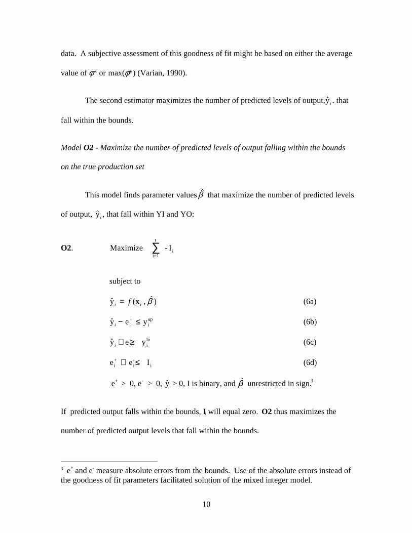
Model O2 - Maximize the number of predicted levels of output falling within the bounds

on the true production set

This model finds parameter values $β that maximize the number of predicted levels

of output, $y i , that fall within YI and YO:

O2. Maximize - Iii=1

t

∑

subject to

$ ( , $)y i if= x β (6a)

$y i − ≤e yi+

iup (6b)

$y i + ≥e yi-

ilo (6c)

e e Ii+

i-

i+ ≤ (6d)

e+ > 0, e- > 0, $y > 0, I is binary, and $β unrestricted in sign.3

If predicted output falls within the bounds, Ii will equal zero. O2 thus maximizes the

number of predicted output levels that fall within the bounds.

3 e+ and e- measure absolute errors from the bounds. Use of the absolute errors instead ofthe goodness of fit parameters facilitated solution of the mixed integer model.

11

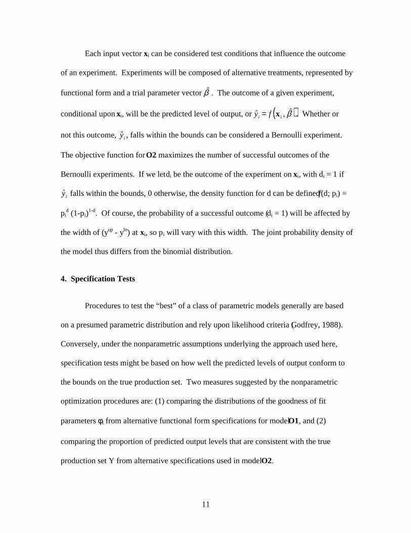
Each input vector xi can be considered test conditions that influence the outcome

of an experiment. Experiments will be composed of alternative treatments, represented by

functional form and a trial parameter vector $β . The outcome of a given experiment,

conditional upon xi, will be the predicted level of output, or ( )$ , $y fi = x i β . Whether or

not this outcome, $yi , falls within the bounds can be considered a Bernoulli experiment.

The objective function for O2 maximizes the number of successful outcomes of the

Bernoulli experiments. If we let di be the outcome of the experiment on xi, with di = 1 if

$yi falls within the bounds, 0 otherwise, the density function for d can be defined f(d; pi) =

pid (1-pi)

1-d. Of course, the probability of a successful outcome (di = 1) will be affected by

the width of (yup - ylo) at xi, so pi will vary with this width. The joint probability density of

the model thus differs from the binomial distribution.

4. Specification Tests

Procedures to test the “best” of a class of parametric models generally are based

on a presumed parametric distribution and rely upon likelihood criteria (Godfrey, 1988).

Conversely, under the nonparametric assumptions underlying the approach used here,

specification tests might be based on how well the predicted levels of output conform to

the bounds on the true production set. Two measures suggested by the nonparametric

optimization procedures are: (1) comparing the distributions of the goodness of fit

parameters φi from alternative functional form specifications for model O1, and (2)

comparing the proportion of predicted output levels that are consistent with the true

production set Y from alternative specifications used in model O2.

12

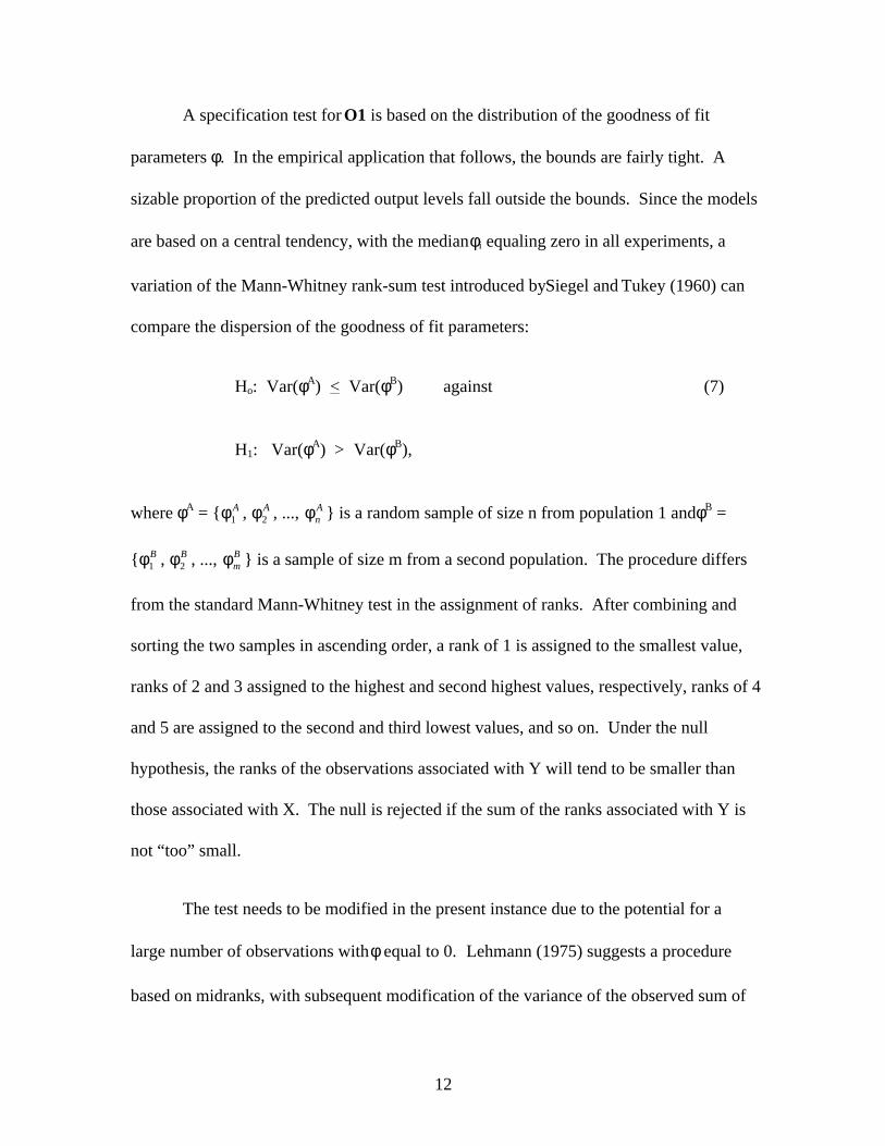
A specification test for O1 is based on the distribution of the goodness of fit

parameters φ. In the empirical application that follows, the bounds are fairly tight. A

sizable proportion of the predicted output levels fall outside the bounds. Since the models

are based on a central tendency, with the median φi equaling zero in all experiments, a

variation of the Mann-Whitney rank-sum test introduced by Siegel and Tukey (1960) can

compare the dispersion of the goodness of fit parameters:

Ho: Var(φA) < Var(φB) against (7)

H1: Var(φA) > Var(φB),

where φA = {φ1A , φ2

A , ..., φnA } is a random sample of size n from population 1 and φB =

{φ1B , φ2

B , ..., φmB } is a sample of size m from a second population. The procedure differs

from the standard Mann-Whitney test in the assignment of ranks. After combining and

sorting the two samples in ascending order, a rank of 1 is assigned to the smallest value,

ranks of 2 and 3 assigned to the highest and second highest values, respectively, ranks of 4

and 5 are assigned to the second and third lowest values, and so on. Under the null

hypothesis, the ranks of the observations associated with Y will tend to be smaller than

those associated with X. The null is rejected if the sum of the ranks associated with Y is

not “too” small.

The test needs to be modified in the present instance due to the potential for a

large number of observations with φ equal to 0. Lehmann (1975) suggests a procedure

based on midranks, with subsequent modification of the variance of the observed sum of

13

ranks to account for the number of ties within the two samples. The resulting statistic W*

is a generalization of the rank sum W. The test is then based on the standard normal

approximation,

( )[ ]( )z

W E W

Var W*

* *

*=

−(8)

where E(W*) = 0.5n(N+1) and

( ) ( )Var W

mnmn d di i

i

e

( )* = −−

=∑

N +1

N(N -1)12 12

3

1 (9)

where the N = m + n observations take on e distinct values. The parameter di, i = 1, ..., e,

equals the number of ties in group i. It is easy to see that, when no ties are present, all di

equal 1, and Var(W*) equals the variance of W, the sum of ranks from a continuous

sample.

With respect to the proportion of predicted levels of output that fall within the

bounds resulting from O2, evidence might support a particular specification if the number

of such hits is significantly greater than the hits experienced under another specification, or

Ho: pA > pB. A 2×2 contingency table results in the test statistic T, which is distributed as

a χ2 distribution with 1 degree of freedom (Mendenhall and Schaeffer, 1973). Denoting

successes as Si, i = 1,2, failures as Fi, and the number of observations in each sample as ni,

the test statistic η is

14

( )( )( )( )η =

+ −

+ +

n n S F F S

n n S S F F

1 2 1 2 1 2

2

1 2 1 2 1 2

(10)

A one-tailed test can be conducted to determine if the specification yielding the larger

number of hits is significantly better at predicting output levels consistent with the true

production set.

5. An Illustration of the Procedures

We employ the Tornquist-Theil indexes of quantities and prices for the U.S.

agricultural sector between 1948 and 1983 compiled by Capalbo and Vo (1988) for an

empirical demonstration of the procedures. These data have been used extensively in

production analysis (Capalbo, 1988; Chavas and Cox, 1995; Lambert and Shonkwiler,

1995). Nonparametric tests of various technical and behavioral conditions will indicate

appropriate restrictions to impose prior to estimation of the alternative production

function specifications.

Testing the data for separability, profit maximization, scale, and regularity conditions

Capalbo and Vo (1988) report indexes for 10 inputs: family labor, hired labor,

land, structures, other capital, energy, fertilizer, pesticides, feed, and miscellaneous items.

To facilitate econometric estimation, inputs are generally aggregated into a smaller number

of categories. However, separability is often a maintained, rather than tested, hypothesis.

Varian (1984) provides a nonparametric test for determining the existence of sub-

production functions for input subsets that would justify aggregation. Differentiating the

total input vector into two subvectors, (x, z), and similarly partitioning the price vector

15

into (r, v), a production function f(x, z) is weakly separable in z if there exists a

production function h(z) and an aggregator function g(x, h) such that f(x, z) = g(x, h(z)).

Testing for the separability of z involves finding values of the numbers φi, λi > 0 for all i =

1,..., t such that φi < φj + λj vj (zi-zj) (Varian, 1984, p. 588). Four linear programming

problems consistent with four input aggregates (labor, land and structures, other capital,

and materials) were solved to find values of φi, λi > 0 satisfying the inequality. Feasible

solutions for all four problems were obtained, indicating the data are consistent with the

separability assumption.

Consistency with WAPM is both necessary and sufficient for the existence of a

true production possibilities set that p-rationalizes the observed data (Varian, 1984). Lack

of consistency with WAPM can arise either through measurement error or from structural

changes, such as technical change, affecting the nature of the production possibilities set.

Recall the test for WAPM: piyi - rixi > piyj - rixj for all i, j = 1, ..., n. Measurement error

can affect both forward (i<j) and backward (i>j) comparisons (Varian, 1985). In the

presence of nonregressive technical change, inconsistency with WAPM will appear in

forward comparisons (i<j). In backward comparisons of the data, 3.5 % (or 23 of the 666

comparisons) violated WAPM. Varian (1985) developed a test to suggest whether

violations of WAPM support rejection of the joint hypothesis of a convex technology,

monotonic technical change, and profit maximization or could have arisen from

measurement error. Employing these procedures resulted in a critical value of 0.532

percent at the 10 percent level of significance. To interpret this value, one can reject the

joint null if there is a reason to believe that the data were measured with less than 0.532

16

percent error. We might reasonably presume that the data were not measured with less

than 0.532 percent error, and can thus be somewhat confident in not rejecting the null in

comparing production sets with earlier periods.

There were 605 violations (90.8 percent) in forward comparisons of the data (i<j),

The corresponding critical value for the minimum standard error was 5.42 percent, again

at the 10 percent significance level. Since it is conceivable that the data could have been

reported with less than 5.42 percent error, we might reject the joint null. Specifically, we

concentrate on the likely presence of nonregressive technical change over this period being

responsible for the inconsistency with WAPM. This decision was based on substantial

evidence supporting technical advance in U.S. agricultural production over this period

(Lambert and Shonkwiler, 1995; Alston and Pardey, 1996). Consequently, the data were

modified to account for production changes over the period.

Several alternative procedures exist to augment both factors and products to

incorporate technical change. Chavas and Cox (1990, 1992, 1995) have adopted the

translating hypothesis developed in Pollak and Wales (1981) to derive via linear

programming techniques factor and product augments representing technical change. The

translating hypothesis asserts that effective outputs y*t and inputs x*t are related to

observed levels by the linear augments, at and bt, or y*t = yt + at and x*t = xt + bt.

Augmentation factors are sought that result in consistency with WAPM, or piy*i-rix*i >

piy*j-rix*j, i , j = 1,...,t. Values of a and b that satisfy the inequalities for all i and j indicate

the existence of a true production function over the entire period (Varian, 1984, theorem

14). Chavas and Cox (1992, 1995) recommend solving the set of T(T-1) linear equations

17

by appending an objective function that minimizes a weighted measure of the deviations of

the effective netputs from the netput levels observed in the sample, or Minimize

( )k ka bta bt t+∑ . The scalars ka and kb differentially weight the factor augments for

output and inputs. We follow Chavas and Cox in using ka = 1000 and kb = ka2.

By construction, the effective netputs satisfy WAPM. Consequently, there does

exist a continuous, concave, monotonic production function that p-rationalizes the

effective netputs. Further properties (homogeneity and homotheticity) of the effective

netput production set can be tested using nonparametric procedures. The nonparametric

test for linear homogeneity requires piyi - rixi = 0 for all i = 1, ..., n. Although this is a

strict requirement and admits of no error in its strictest interpretation, (piy*i)/(rix*i) ranged

from 1.98 to 0.81. These estimates are again made without distributional information, but

the wide range of values rule out functional forms which impose linear homogeneity.

Finally, Varian’s (1984) test for homotheticity requires finding feasible solutions to

the system of equations φi < φj vjxi for φi > 0, i, j = 1, ..., n, where vi = wi/wixi. The

effective netputs satisfied the nonparametric test for homotheticity.

As a result of these nonparametric tests, we may thus consider parametric

representations that are continuous, monotonic, concave, and homothetic. Homotheticity

can either be imposed in the functional form, or specifications satisfying homotheticity

automatically can be chosen. In some cases, such as the Cobb-Douglas, concavity can be

imposed directly. In other cases, such as the translog, concavity cannot be imposed, but

18

tests of concavity can be conducted for given parameter vectors by evaluating the Hessian

of the estimated production function.

Since the 1948-1983 effective netput vectors are consistent with WAPM, YO, YI,

and Y coincide at these observations.4 Upper and lower bounds on the true output levels

associated with unobserved input vectors can then be established by new input vectors

using Varian’s results. Consequently, convex combinations of the 36 original effective

input vectors were formed, and models [2] and [3] were solved for each of these

generated input vector to derive corresponding values for yup and ylo. The original 36

effective netput bundles were thus augmented by an additional 275 vectors of inputs and

associated upper and lower bounds on the corresponding output levels

6. Results

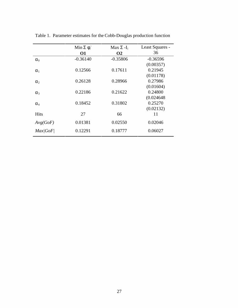
Three functional forms were estimated, the Cobb-Douglas, the translog, and the

generalized Leontief (Denny, 1974), using models O1 and O2. For comparison, a single

equation least squares estimation was conducted over the 1948-1983 effective netput

bundles for the three functional specifications. Coefficient estimates are reported in tables

1-3. Specification tests resulting from comparisons of the dispersion of the goodness of fit

parameters (O1) and the tests for equal proportions of hits (O2) are reported in table 4.

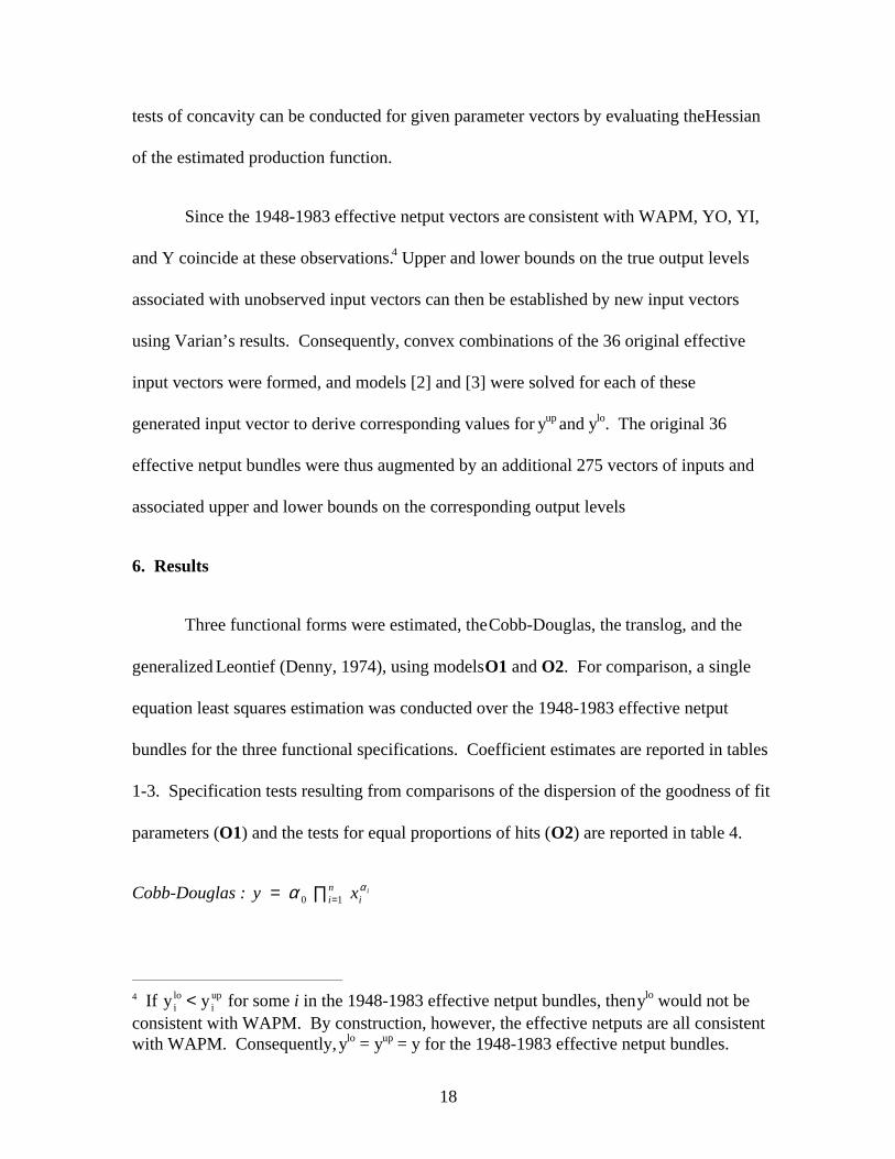
Cobb-Douglas : y xin

ii= ∏ =α α

0 1

4 If y yi

loiup< for some i in the 1948-1983 effective netput bundles, then ylo would not be

consistent with WAPM. By construction, however, the effective netputs are all consistentwith WAPM. Consequently, ylo = yup = y for the 1948-1983 effective netput bundles.

19

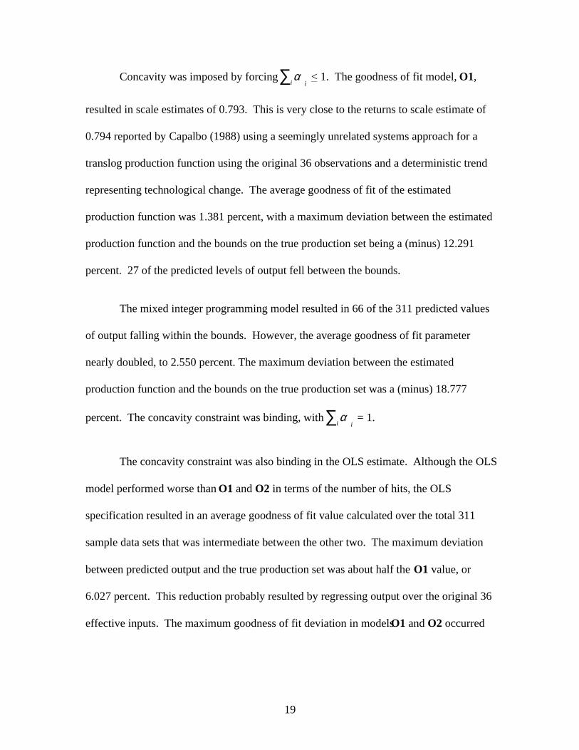
Concavity was imposed by forcing αi i

∑ < 1. The goodness of fit model, O1,

resulted in scale estimates of 0.793. This is very close to the returns to scale estimate of

0.794 reported by Capalbo (1988) using a seemingly unrelated systems approach for a

translog production function using the original 36 observations and a deterministic trend

representing technological change. The average goodness of fit of the estimated

production function was 1.381 percent, with a maximum deviation between the estimated

production function and the bounds on the true production set being a (minus) 12.291

percent. 27 of the predicted levels of output fell between the bounds.

The mixed integer programming model resulted in 66 of the 311 predicted values

of output falling within the bounds. However, the average goodness of fit parameter

nearly doubled, to 2.550 percent. The maximum deviation between the estimated

production function and the bounds on the true production set was a (minus) 18.777

percent. The concavity constraint was binding, with αi i

∑ = 1.

The concavity constraint was also binding in the OLS estimate. Although the OLS

model performed worse than O1 and O2 in terms of the number of hits, the OLS

specification resulted in an average goodness of fit value calculated over the total 311

sample data sets that was intermediate between the other two. The maximum deviation

between predicted output and the true production set was about half the O1 value, or

6.027 percent. This reduction probably resulted by regressing output over the original 36

effective inputs. The maximum goodness of fit deviation in models O1 and O2 occurred

20

over the original 36 effective netput bundles. Fitting the production function to just these

bundles using OLS reduced this maximum deviation.

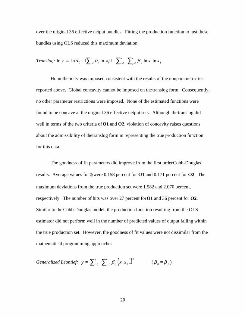
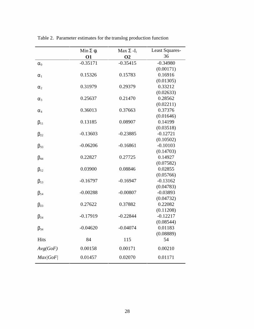
Translog: ln ln ln ln lny x x xii

n

i i

n

ij i jj

n= + += = =∑ ∑ ∑α α β0 1 1 1

Homotheticity was imposed consistent with the results of the nonparametric test

reported above. Global concavity cannot be imposed on the translog form. Consequently,

no other parameter restrictions were imposed. None of the estimated functions were

found to be concave at the original 36 effective netput sets. Although the translog did

well in terms of the two criteria of O1 and O2, violation of concavity raises questions

about the admissibility of the translog form in representing the true production function

for this data.

The goodness of fit parameters did improve from the first order Cobb-Douglas

results. Average values for φ were 0.158 percent for O1 and 0.171 percent for O2. The

maximum deviations from the true production set were 1.582 and 2.070 percent,

respectively. The number of hits was over 27 percent for O1 and 36 percent for O2.

Similar to the Cobb-Douglas model, the production function resulting from the OLS

estimator did not perform well in the number of predicted values of output falling within

the true production set. However, the goodness of fit values were not dissimilar from the

mathematical programming approaches.

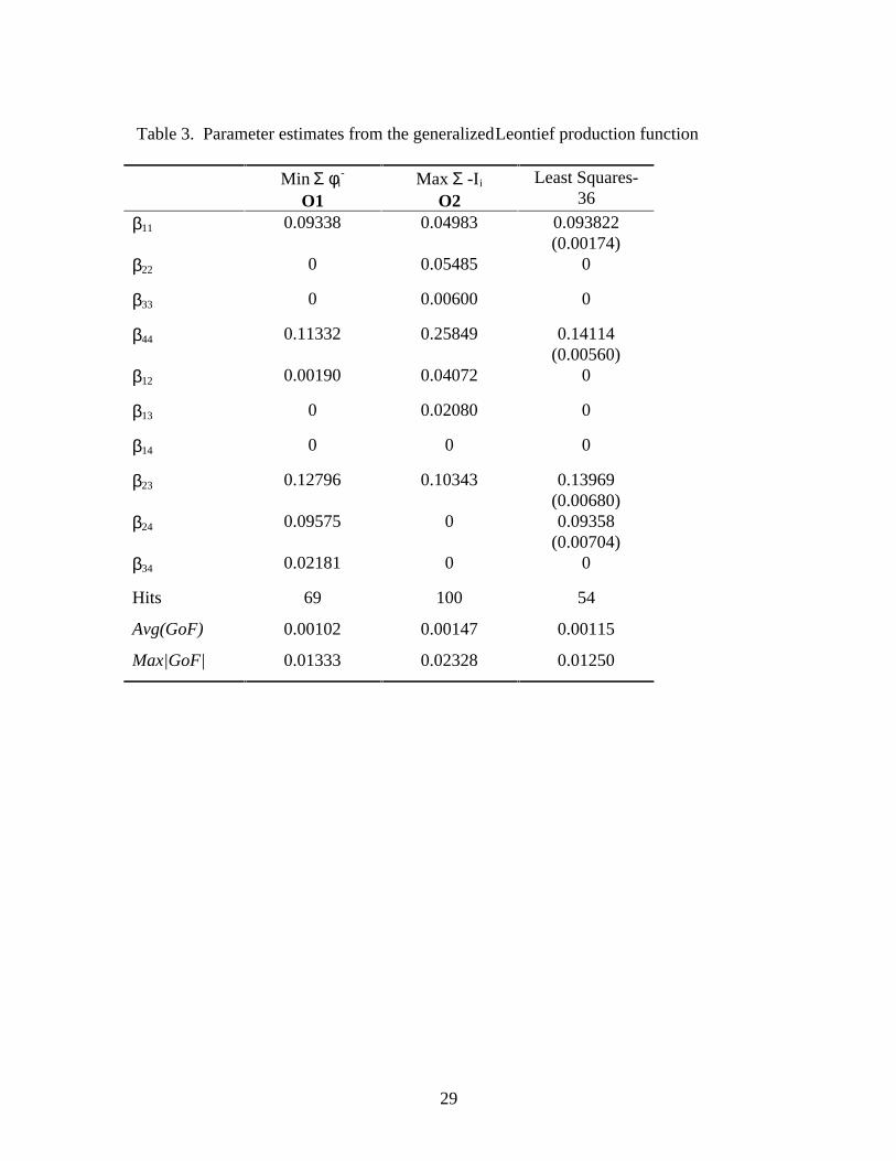
Generalized Leontief: ( )y x xi

n

ij i jj

n= = =∑ ∑1

1 2

1β ( β βij ji= )

21

The generalized Leontief function is linearly homogeneous by construction.

Concavity is imposed by setting β ij ≥ 0 . The goodness of fit parameters and the number

of hits resulting from the GL model are similar to the results from the translog model.

Comparisons of Functional Forms

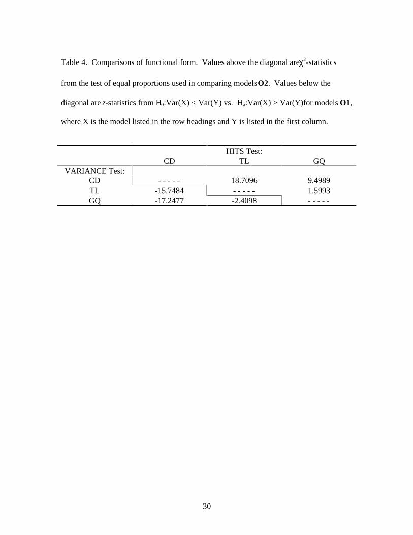
Nonparametric test results for the three models are in Table 4. Both the TL and

the GL register a significantly higher number of predicted levels of output falling within

the true production set than the CD. The proportion of hits registered by the TL is higher

than the GL (115 vs. 100), but the hypothesis of equal proportions could not be rejected

for probabilities greater than about 0.10. Measures of the dispersion of the goodness of fit

parameters (model O1) from the true production set yield similar results. The null is

soundly rejected with respect to the CD-TL and the CD-GL comparisons. The null is also

rejected in the comparison of the goodness of fit parameters from the TL and the GL

models (z = -2.4098). The variance of the φ vector associated with the TL is greater than

the variance for the GL model.

The results relative to the CD are not surprising given that the CD is a first-order

approximation. Comparisons of the TL and the GL are mixed. The TL form resulted in

more predicted levels of output falling within the bounds of the true production set,

though the difference was not significant using the test of equal proportions. The

dispersion of the goodness of fit parameters of the GL was less than the dispersion

associated with the TL at greater than the 99 percent level of significance.

22

Since the theme underlying this work has been the distinction between statistical

significance and the consistency of estimated functional specifications with economic

behavior, we would tend to prefer the generalized Leontief form over the translog. Since

the best TL specifications under both O1 and O2, as well as the OLS models, failed to

satisfy concavity, we would prefer to accept the GL as a specification that satisfies the

restrictions on the true production set resulting from the series of nonparametric tests

conducted prior to estimation.

7. Summary

A procedure was developed in this paper in which the bounds on the true

production set allows augmenting observed data sets with observations that are consistent

with profit maximizing behavior. Continuous production functions can then be estimated

over this data set that is known to bound the true production set. Because of the

discontinuous nature of the bounded production set, a system of inequality constraints in

quantity space formed the feasible region for two alternative mathematical programming

models used to estimate parameters of alternative specifications. Goodness of fit tests

were used to compare consistency of the predicted outputs with the true production set.

The generalized Leontief specification was considered best in terms of satisfying known

characteristics of the true production function, namely concavity. The average goodness

of fit of the generalized Leontief was between 0.10 (model O1) and 0.15 (model O2)

percent, which falls well within the 5 percent suggested by Varian (1985) as adequate

levels of acceptance for this nonparametric estimation.

23

This paper has made two contributions. First, a given data set can be augmented

by generating additional netput vectors that bound the true production set. Procedures to

establishing these bounds is attributed to Varian (1984). However, we developed

procedures in this paper to estimate production functions consistent with the known

characteristics of these constructed netput vectors. The second contribution has been to

propose a mathematical programming estimator for maximizing goodness of fit, not to

statistical criteria, but to the criteria suggested by neoclassical production theory.

24

References

Afriat, S., 1972, Efficiency estimates of production functions, International Economic

Review 13, 568-598.

Alston, J.M., and P.G. Pardey, 1996, Making Science Pay: The Economics of Agricultural

R&D Policy (The AEI Press, Washington, D.C.).

Capalbo, S. M., 1988, A comparison of econometric models of U.S. agricultural

productivity and aggregate technology, in: S.M. Capalbo and J. Antle, eds., Agricultural

Productivity: Measurement and Explanation (Resources for the Future Press, Washington

D.C.) 159-188.

__________ and T.T. Vo, 1988, A review of the evidence on agricultural productivity

and aggregate technology, in: S.M. Capalbo and J. Antle, eds., Agricultural Productivity:

Measurement and Explanation (Resources for the Future Press, Washington D.C.) 96-

137.

Charnes, A., W.W. Cooper, B. Golany, and L. Seiford, 1985, Foundations of data

envelopment analysis for Pareto-Koopmans efficient empirical production functions,

Journal of Econometrics 30, 91-107.

Chavas, J. P. and T. L. Cox, 1990, A nonparametric analysis of productivity: the case of

U.S. and Japanese manufacturing, American Economic Review 80, 450-464.

25

___________, 1992, A nonparametric analysis of the influence of research on agricultural

productivity, American Journal of Agricultural Economics 74, 583-591.

___________, 1995, On nonparametric supply response analysis, American Journal of

Agricultural Economics 77, 80-92.

Denny, M., 1974, The relationship between functional forms for the production system,

Canadian Journal of Economics 7, 21-31.

Fare&& , R.. and S. Grosskopf, 1985, A nonparametric cost approach to scale efficiency,

Scandinavian Journal of Economics 87, 594-604.

_____________, 1995, Nonparametric tests of regularity, Farrell efficiency, and goodness

of fit, Journal of Econometrics 69, 415-425.

_____________ and C.A. Knox Lovell, 1994, Production Frontiers (Cambridge

University Press, Cambridge, U.K.).

Godfrey, L. G., 1988, Misspecification Tests in Econometrics (Cambridge University

Press: Cambridge, U.K.).

Hanoch, G. and M. Rothschild, 1972, Testing the assumptions of production theory: a

nonparametric approach, Journal of Political Economy 80, 256-275.

Lambert, D. K. and J. S. Shonkwiler, 1995, Factor bias under stochastic technical change,

American Journal of Agricultural Economics 77, 578-590.

26

Lambert, D.K., 1996, On nonparametric supply response analysis: comment. American

Journal of Agricultural Economics 78.

Lehman, E.L., 1975, Nonparametrics: Statistical Methods Based on Ranks (Holden-Day

Inc.: San Francisco).

Mendenhall, W., and R.L. Schaeffer, 1973, Mathematical Statistics with Applications

(Duxbury Press: North Scituate, MA).

Pollak, R.A., and T.J. Wales, 1981, Demographic variables in demand analysis,

Econometrica 49, 1533-1551.

Shumway, C. R. and H. Lim, 1993, Functional form and U.S. agricultural production

elasticities, Journal of Agricultural and Resource Economics 18, 266-276.

Siegel, S. and J. W. Tukey, 1960. A nonparametric sum of ranks procedure for relative

spread in unpaired samples, Journal of the American Statistical Association 55, 429-444.

Errata: Ibid., 1961, 1005 (5.3).

Varian, Hal R., 1984, The nonparametric approach to production analysis, Econometrica

52, 579-597.

____________, 1985, Non-parametric analysis of optimizing behavior with measurement

error, Journal of Econometrics 30, 445-458.

____________, 1990, Goodness-of-fit in optimizing models, Journal of Econometrics 46,

125-140.

27

Table 1. Parameter estimates for the Cobb-Douglas production function

Min Σ φi-

O1Max Σ -Ii

O2Least Squares -

36

α0 -0.36140 -0.35806 -0.36596(0.00357)

α1 0.12566 0.17611 0.21945(0.01178)

α2 0.26128 0.28966 0.27986(0.01604)

α3 0.22186 0.21622 0.24800(0.024648

α4 0.18452 0.31802 0.25270(0.02132)

Hits 27 66 11

Avg(GoF) 0.01381 0.02550 0.02046

Max|GoF| 0.12291 0.18777 0.06027

28

Table 2. Parameter estimates for the translog production function

Min Σ φi

O1Max Σ -Ii

O2Least Squares-

36

α0 -0.35171 -0.35415 -0.34980(0.00171)

α1 0.15326 0.15783 0.16916(0.01305)

α2 0.31979 0.29379 0.33212(0.02633)

α3 0.25637 0.21470 0.28562(0.02211)

α4 0.36013 0.37663 0.37376(0.01646)

β11 0.13185 0.08907 0.14199(0.03518)

β22 -0.13603 -0.23885 -0.12721(0.10502)

β33 -0.06206 -0.16861 -0.10103(0.14703)

β44 0.22827 0.27725 0.14927(0.07582)

β12 0.03900 0.08846 0.02855(0.05766)

β13 -0.16797 -0.16947 -0.13162(0.04783)

β14 -0.00288 -0.00807 -0.03893(0.04732)

β23 0.27622 0.37882 0.22082(0.11208)

β24 -0.17919 -0.22844 -0.12217(0.08544)

β34 -0.04620 -0.04074 0.01183(0.08889)

Hits 84 115 54

Avg(GoF) 0.00158 0.00171 0.00210

Max|GoF| 0.01457 0.02070 0.01171

29

Table 3. Parameter estimates from the generalized Leontief production function

Min Σ φi-

O1Max Σ -Ii

O2Least Squares-

36

β11 0.09338 0.04983 0.093822(0.00174)

β22 0 0.05485 0

β33 0 0.00600 0

β44 0.11332 0.25849 0.14114(0.00560)

β12 0.00190 0.04072 0

β13 0 0.02080 0

β14 0 0 0

β23 0.12796 0.10343 0.13969(0.00680)

β24 0.09575 0 0.09358(0.00704)

β34 0.02181 0 0

Hits 69 100 54

Avg(GoF) 0.00102 0.00147 0.00115

Max|GoF| 0.01333 0.02328 0.01250

30

Table 4. Comparisons of functional form. Values above the diagonal are χ2-statistics

from the test of equal proportions used in comparing models O2. Values below the

diagonal are z-statistics from H0:Var(X) < Var(Y) vs. Ha:Var(X) > Var(Y)for models O1,

where X is the model listed in the row headings and Y is listed in the first column.

HITS Test:CD TL GQ

VARIANCE Test:CD - - - - - 18.7096 9.4989TL -15.7484 - - - - - 1.5993GQ -17.2477 -2.4098 - - - - -