A Proposal for Network Air Traffic Flow Management

Incorporating Fairness and Airline Collaboration∗

Dimitris Bertsimas† Shubham Gupta‡

April 25, 2011

Abstract

There has been significant research effort in the academic literature related to AirTraffic Flow Management (ATFM). Yet, the research has not been fully implemented inpractice. In our opinion, the key reasons are - i) the existing network models approach theproblem from the point of view of a central decision-maker without taking into accountthe airlines to a significant degree; and ii) the notions of fairness as introduced under theCollaborative Decision-Making (CDM) paradigm operate under a single-airport settingand do not address network effects (presence of multiple airports, sectors and variousconnectivity requirements). In this paper, we address these shortfalls by presenting aproposal which alleviates both these concerns. In stage I of our proposal, we presentnetwork models that incorporate a notion of fairness - controlling number of reversalsand total amount of overtaking. In stage II, we allow for further airline collaborationby proposing a network model for slot reallocation. We provide empirical results of theproposed optimization models on national-scale, real world datasets spanning across sixdays that show interesting tradeoffs between fairness and efficiency. We report promisingcomputational times of less than 30 minutes for up to 25 airports and provide theoreticalevidence that illuminates the strength of our formulations.

1 Introduction

The sustained growth of the aviation industry has put a tremendous strain on the availableresources of the air transporation system. This is evidenced by the steady increase in flightdelays and severe congestion at airports. In 2008, approximately 22% of the flights in theUnited States were delayed by more than 15 minutes, while another 2% were cancelled(Bureau of Transportation Statistics [17]). Moreover, during the 12-month period ending in∗Research funded by the NSF Grant EFRI-0735905.†Boeing Professor of Operations Research, Sloan School of Management, Co-director of the Opera-

tions Research Center, Massachusetts Institute of Technology, E40-147, Cambridge, MA 02139-4307, dbert-sim@mit.edu‡Operations Research Center, Massachusetts Institute of Technology, Cambridge, MA 02139-4307, shub-

hamg@mit.edu

1

September 2008, 138 million minutes of system delay led to an estimated $10 billion in costsfor US airlines [1].

Air Traffic Flow Management (ATFM) refers to the set of strategic processes that tryto reduce congestion costs and support the goal of safe, efficient and expeditious aircraftmovement. ATFM procedures try to resolve local demand-capacity mismatches by adjustingthe aggregate traffic flows to match scarce capacity resources. Ground Delay Programs(GDPs) are one of the most sophisticated ATFM initiatives currently in use that attemptto address airport arrival capacity reductions. Under this mechanism, delays are appliedto flights at their origin airports that are bound for a common destination airport which issuffering from reduced capacity or excessive demand. The premise for this tool is that itis better to absorb delays for a flight while it is grounded at its origin airport rather thanincurring air-borne delay near the affected destination airport which is both unsafe and morecostly (in terms of fuel costs). Airspace-Flow Programs (AFPs) are another tool that wereintroduced recently in 2007 and are similar to GDPs in terms of operational details. FAAuses this tool to control arrival rate into a Flow Constrained Area (FCA), e.g., a weatheraffected segment of the airspace. Some of the other ATFM tools include assigning air-bornedelays, dynamic re-routing and speed control. We briefly review the literature on the existingATFM tools below.

Odoni [12] first conceptualized the problem of scheduling flights in real time in order tominimize congestion costs. Thereafter, several models have been proposed to handle differentversions of the problem. The problem of assigning ground-delays in the context of a single-airport (Single-Airport Ground-Holding Problem) has been studied in Terrab and Odoni [15],Richetta and Odoni [13], [14]; and in the multiple airport setting (Multi-Airport Ground-Holding Problem) in Terrab and Paulose [16], Vranas et al. [20]. The problem of controllingrelease times and speed adjustments of aircraft while air-borne for a network of airportstaking into account the capacitated airspace (Air Traffic Flow Management Problem) hasbeen studied in Bertsimas and Stock [5], Helme [9], Lindsay et al. [11]. The problem withthe added complication of dynamically re-routing aircrafts (Air Traffic Flow ManagementRerouting Problem) was first studied by Bertsimas and Stock [6]. Recently, Bertsimas etal. [7] have presented a new mathematical model for the ATFM problem with dynamic re-routing which has superior computational performance. For a detailed survey of the variouscontributions and a taxonomy of all the problems, see Bertsimas and Odoni [4] and Hoffman etal. [10]. It is important to highlight that network formulations present significant challengesof computational tractability, and so far few network models have been able to incorporateequity considerations effectively. Despite the significant progress outlined here, this set ofliterature while addressing network effects (presence of multiple airports, sectors and variousconnectivity requirements), takes the point of view of a single decision-maker and does notaddress the issue of fairness among airlines.

We review next some other important concepts in the ATFM literature - namely, Col-laborative Decision-Making (CDM) and Ration-by-Schedule (RBS). The decision-making re-

2

sponsibilities in ATFM initiatives are shared between a number of stakeholders (primarily,airlines and the FAA). This poses a major challenge as their actions are highly interdepen-dent and demand real-time exchange of information between the FAA and the airlines. Thisrealization of enhanced cooperation between the various stakeholders led to the adoption ofCollaborative Decision-Making (CDM) philosophy (Ball et al. [2], Wambsganss [21]) by theFAA in the 1990s. Under CDM, all ATFM initiatives are conducted in a way that gives sig-nificant decision-making responsibilities to airspace users (see Hoffman et al. [10] for detailson CDM). All recent efforts to improve ATFM have been guided by this philosophy. In theUS, “Ration-by-Schedule” (RBS) is the fundamental principle for all the CDM initiatives.Under this paradigm - arrival slots at airports are assigned to flights in accordance with afirst-scheduled, first-served (FSFS) priority discipline (see Ball et al. [2], Wambsganss [21]for details on rationing). In the case of GDP and AFP planning, all stakeholders have agreedthat this principle is fair to all parties. This allocation process is followed by a Compressionalgorithm, which fills open slots created by flights that are canceled. The compression pro-cedure gives airlines an incentive to report accurate flight information, by rewarding themfor reporting cancellations. The combined process, RBS plus Compression (formally calledRBS++) is the policy currently in use for slot allocations. Despite the use of RBS in a GDPsetting, there have been no network models that satisfy the RBS principle in a multi-airportsetting. This is because, applying RBS to each of the airports individually might not lead toa schedule that preserves time, sector and flight connectivities. In addition, the impositionof a maximum permissible delay on each flight (as required by any tractable optimizationmodel) would mean that a feasible solution under RBS might not even exist if the capacityreduction at some airports is significant. Hence, there is no straightforward extension ofRBS from a single-airport setting to an airspace context. As part of the CDM philosophy,researchers have also explored dynamic interaction with airlines. Towards this aim, Vossenand Ball [19] [18] have studied opportunities for slot trading in a single-airport setting wherethe aim is to formalize an optimization problem for the FAA given the offers to trade fromvarious airlines. In summary, the CDM concepts discussed here while addressing the issuesof fairness among airlines in a single-airport setting, do not address network effects.

Our goal in this paper is to propose an optimization based approach that a) incorporatesnetwork effects and builds upon the ATFM literature; and b) takes into account fairness con-siderations among airlines by building upon the CDM philosophy. Specifically, our proposalconsists of the following two stages:

Stage I - Network ATFM model incorporating fairness:We generalize the classical ATFM models ([5]) to incorporate fairness considerations forairlines. The objective function used in the existing network ATFM models is to minimize thetotal delay costs across all flights, i.e., the focus is on overall system efficiency. A disadvantageof such an approach is that the solution to such models can have a large number of reversals,i.e., the resulting order of flight arrivals can be quite different as compared to the publishedflight schedules. Specifically, for two flights f and f ′ arriving at the same destination airport,a reversal occurs if f was scheduled to arrive before f ′ but f ′ arrives before f in the actual

3

schedule. Moreover, across these reversals, there might be different number of time-periodsof overtaking. Concretely, the duration between the arrival of flights f ′ and f constitutethe amount of overtaking. Consequently, the total overtaking across these reversals mightbe large. Because of this deviation from the original flight ordering, it becomes difficult toimplement such a solution because of the coupling in the crew assignments and the use ofhub and spoke networks. We propose discrete optimization models that add these fairnesscontrols. The key output in this stage is the assignment of flights to different time periods.

Stage II - Slot reallocation through airline collaboration:We generalize the notion of intra-airline exchange of arrival slots, a key component of thecurrent CDM practice in a single-airport setting to network-wide slot reallocation amongairlines. Specifically, we propose an optimization model which takes as input the assignmentof flights to different time periods from Stage I and permits the airlines to trade these assignedslots across different airports, thereby, resulting in improved internal objective functions. Themodel proposed for Stage II of our proposal allows airlines to react to the schedule determinedin Stage I by taking into account their flights in the entire network and making appropriatetradeoffs.

Contributions of this work

We feel our work makes the following contributions:

1. We present a proposal for the network ATFM problem which incorporates both fairnessand airline collaboration while operating under a broad CDM paradigm. Specifically,we formulate discrete optimization models to impose fairness controls in Stage I and amodel for slot reallocation in Stage II.

2. We provide empirical results of the proposed optimization models on national-scale, realworld datasets spanning across six days. We report promising computational times ofless than 30 minutes for up to 25 airports and provide theoretical evidence on thestrength of our formulations.

Simultaneously, Barnhart et al. [3] develop an alternative way to address fairness in thecontext of ATFM. They develop a fairness metric that measures deviation from FSFS andpropose a discrete optimization model that directly minimizes this metric. They furtherdevelop an exponential penalty approach, and report encouraging computational results usingsimulated regional and national scenarios. In contrast to this work, our paper differs in thefollowing respects: a) we provide an exact method to model overtaking within a mathematicalprogramming framework while [3] proposes an approximate method. In addition, we proposeanother, although related, metric of fairness - controlling the number of reversals; b) weexplicitly model network effects that [3] does not; and c) our proposal consists of a slotreallocation phase (Stage II) which enables airlines to implicitly trade their internal objective

4

functions to derive more utility. In summary, both papers contribute to the understandingof fairness in ATFM by approaching the problem from distinct perspectives.

Organization of the paper

Section 2 summarizes an adaptation of the Bertsimas Stock-Patterson model [5] in order toaccommodate our proposal. Section 3 introduces models of fairness. Section 4 introducesour model of slot reallocation. Section 5 discusses how our proposal can be integratedwith the current CDM practices. Section 6 reports computational results of the proposedoptimization models on six days of national-scale, real world datasets. Section 7 summarizesour conclusions and the Appendix reports polyhedral analysis that illuminates the strengthof our proposed formulations.

2 ATFM Problem: Notation, Bertsimas Stock-Patterson Model

and Solutions

In this section, we reproduce the Bertsimas Stock-Patterson model [5] for the ATFM problemwhich provides the starting point for all the models presented herein. We use an extendedversion of the notation used in that paper in order to accommodate fairness and slot reallo-cation considerations. Finally, we illustrate difficulties relative to fairness considerations inthe solutions obtained from this model.

The Decision Variables

The decision variables are:

wfj,t =

{1, if flight f arrives at sector j by time t,

0, otherwise.

This definition of the decision variables, using “by” instead of “at”, is critical to the under-standing of the formulation. The variables are defined only for the set of sectors an aircraftmay fly through on its route to the destination airports. In addition, variables are used forthe departure and the arrival airports, in order to determine the optimal times for departureand for arrival. Since we do not consider flight cancellations, at least two variables can befixed a priori for each flight: each aircraft has to take off by the end of a feasible time windowand has to land, as well, within a feasible time window, which is determined by the time ofdeparture.

5

Notation

The model’s formulation requires definition of the following notation:

K : set of airports,

F : set of flights,

T : set of time periods,

W : set of airlines,

Fw ⊆ F : set of flights belonging to airline w,

S : set of sectors,

Sf ⊆ S : sequence of sectors flown by flight f,

C : set of pairs of flights that are continued,

Rj : set of pairs of flights that are reversible in resource j (definition below),

RS : set of pairs of flights that are reversible in sectors (definition below),

RA : set of pairs of flights that are reversible at airports (definition below),

Pfi : sector i’s preceding sector in the path of flight f,

Lfi : sector i’s subsequent sector in the path of flight f,

Dk(t) : departure capacity of airport k at time t,

Ak(t) : arrival capacity of airport k at time t,

Sj(t) : capacity of sector j at time t,

df : scheduled departure time of flight f,

ajf : scheduled arrival time of flight f in resource j,

sf : turnaround time of an airplane after flight f,

origf : airport of departure of flight f,

destf : airport of arrival of flight f,

lfj : minimum number of time units that flight f must spend in sector j,

M : maximum permissible delay for a flight,

T fj : set of feasible time periods for flight f to arrive in resource j,

T fj : first time period in the set T fj ,

Tfj : last time period in the set T fj ,

T reversalf,f ′,j : set of time-periods common for flights f and f ′ where a reversal could occur in resource j

(definition below),

Omaxf,f ′,j : maximum amount of overtaking possible between flights f and f ′ in resource j

(definition below),

O : set of all possible trades (definition in Section 4),

Of ⊆ O : set of offers containing flight f,

cf : time period assigned to flight f from Stage I optimization.6

The key additions relative to the notation used in [5] are W, Fw, Rj , RS , RA, T reversalf,f ′,j ,

Omaxf,f ′,j , O, Of ⊆ O and cf .

The sets Rj, RS and RA

We give next the definition of Rj (set of pairs of flights that are reversible in resource j).We make a distinction between the case when the resource j is a sector and when it is anairport.

Definition 2.1. For an airport k ∈ K, a pair of flights (f, f ′) belongs to Rk if the followingtwo conditions are satisfied:

1. destf = destf ′ = k, i.e., the destination airport of both flights f and f ′ is the same.

2. akf ≤ akf ′ ≤ akf + M , i.e., the scheduled time of arrival of flight f ′ at the destinationairport lies between the scheduled time of arrival of flight f and the last time periodin the set of feasible time periods that the flight f can arrive at its destination airport.

Definition 2.2. For a sector j ∈ S, a pair of flights (f, f ′) belongs to Rj if the followingtwo conditions are satisfied:

1. j ∈ Sf and j ∈ Sf ′ , i.e., sector j is common to the path of flights f and f ′.

2. ajf ≤ ajf ′ ≤ a

jf +M , i.e., the scheduled time of arrival of flight f ′ in sector j lies between

the scheduled time of arrival of flight f and the last time period in the set of feasibletime periods that the flight f can arrive in sector j.

For each pair of flights (f, f ′) ∈ Rj , we count a reversal, if in the resulting solution, flightf ′ arrives before flight f in resource j (i.e., ∃t such that wf

′

j,t > wfj,t). We call the reversalsoccurring in sectors as sector reversals and the reversals occurring at the airports as airportreversals. This clustering is motivated from fairness considerations in a network setting andis elaborated upon later in Section 3.

Definition 2.3. The set of pairs of flights that are reversible in sectors (RS) and at airports(RA) is defined as:

1. RS =⋃j∈S Rj

2. RA =⋃k∈KRk

The set T reversalf,f ′,j and parameter Omax

f,f ′,j

Definition 2.4. The set T reversalf,f ′,j (set of time-periods common for flights f and f ′ where a

reversal could occur) is defined as {T f′

j , . . . , Tfj − 1}.

7

To elaborate on Definition 2.4, T reversalf,f ′,j is the set of time-periods t, such that it is possible

to have the following assignment: wfj,t = 0 and wf′

j,t = 1. This assignment would imply thata reversal occurs at time t.

Definition 2.5. The parameter Omaxf,f ′,j is defined as |T reversal

f,f ′,j | (cardinality of the set T reversalf,f ′,j ),

and hence is equal to T fj − Tf ′

j − 1.

To elaborate on Definition 2.4, Omaxf,f ′,j is the maximum amount of overtaking possible

between flights f and f ′ and would be attained when wfj,T

fj−1

= 0 and wf′

j,T f ′j

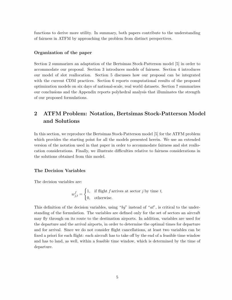
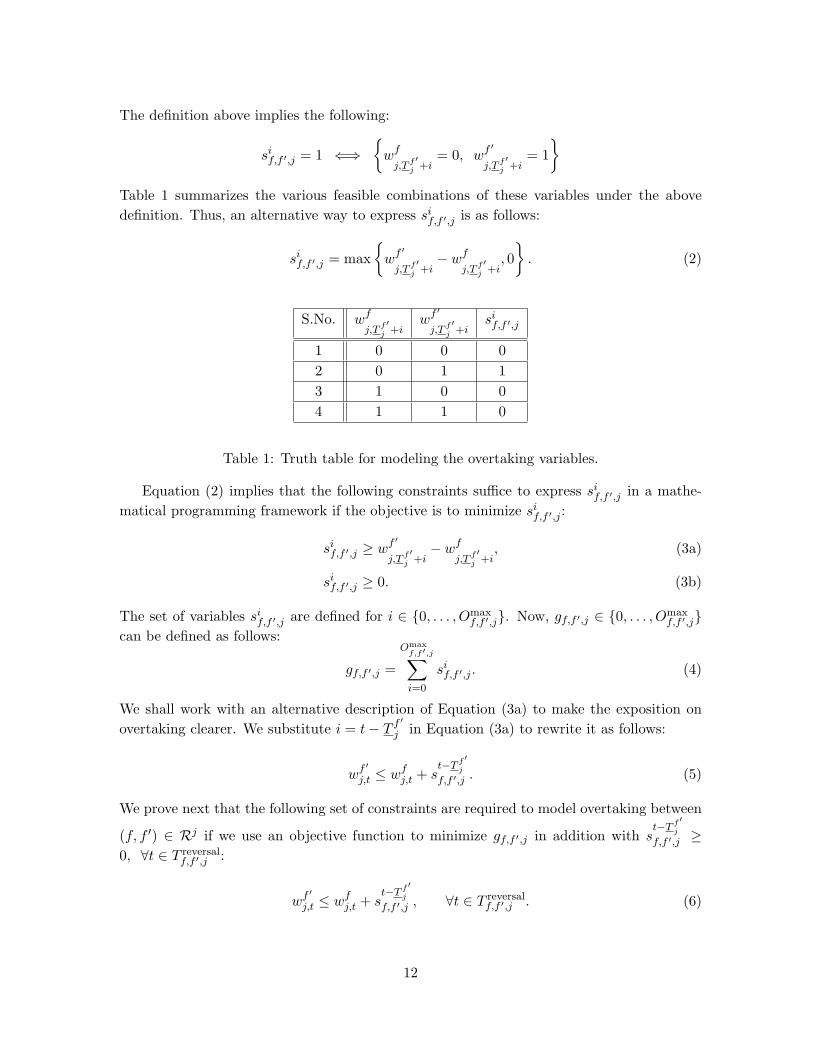
= 1.

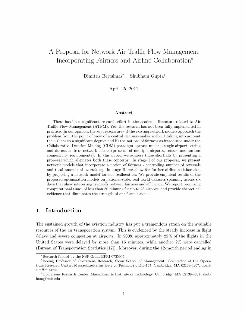
Example 2.1. Figure 1 depicts a reversible pair of flights (f, f ′) ∈ RA. Let destf = destf ′ =k. In this example, the arrows correspond to the set of time-periods common for both flights.Moreover, the set of time-periods marked by these arrows (except for the last one) constituteT reversalf,f ′,k . This is because, the model enforces wf

k,akf+M

= 1 at the outset and hence, it is not

possible to have a reversal at akf +M . Finally, Omaxf,f ′,k = |T reversal

f,f ′,k | = 6.

PSfrag replacementsakf

akf +M

akf ′

akf ′ +M

Feasible times of arrival for flight fFeasible times of arrival for flight f ′

T reversalf,f ′,k

Figure 1: A reversible pair of flights (f, f ′) ∈ RA (destf = k).

The Objective Function

We use an adapted expression for total delay (TD) cost for each flight introduced recentlyin Bertsimas et al. [7]. The total delay (TD) cost is a combination of the costs of air-bornedelay (AD) and ground-holding delay (GD) (TD = GD + α · AD, where α > 1 becauseair-borne delay is typically more costly than ground-holding delay). By substituting AD interms of TD (i.e., AD = TD−GD), the objective can be rewritten as α ·TD− (α− 1) ·GD.

Consequently, the objective function is composed of two terms: a first term that takesinto account the cost of the total delay assigned to a flight and a second term which accountsfor the cost reduction obtained when a part of the total delay is taken as ground delay at

8

the origin airport. The objective function cost coefficients are a super-linear function of thetardiness of a flight of the form (t− akf )1+ε, with ε close to zero. Hence, for each flight f andfor each time period t, we define the following two cost coefficients:

cftotal(t) = α(t− akf )1+ε : total cost of delaying flight f for (t− akf ) units of time,

cfg (t) = (α− 1)(t− df )1+ε : cost reduction obtained by holding flight f on the

ground for (t− df ) units of time,

The motivation of using super-linear cost coefficients is that it will favor moderate assignmentof total delays between two flights rather than assigning much larger delay to one as comparedto the other flight. To elaborate, consider the following example:

Example 2.2. Suppose we wish to assign 2 units of delay to 2 flights. Then, an objectivefunction with linear cost coefficients is equally likely to generate the following two assign-ments: i) 1 unit of delay to both flights and ii) 2 unit of delay to one flight and 0 to theother. In contrast, super-linear cost coefficients (with ε = 0.001 for example) will assign 1unit to both flights because 11.001 + 11.001 < 21.001 + 0.

In view of the above, the delay cost function for each flight f takes the following form: ∑t∈T f

destf

cftotal(t) · (wfdestf ,t

− wfdestf ,t−1)−∑

t∈T forigf

cfg (t) · (wforigf ,t− wforigf ,t−1)

The TFMP model

The complete description of the model, referred to as (TFMP), is as follows:

IZTFMP = min∑f∈F

∑t∈T f

destf

cftotal(t) · (wfdestf ,t

− wfdestf ,t−1)−∑

t∈T forigf

cfg (t) · (wforigf ,t− wforigf ,t−1)

9

subject to:∑f∈F :origf=k

(wfk,t − wfk,t−1) ≤ Dk(t), ∀k ∈ K, t ∈ T . (1a)

∑f∈F :destf=k

(wfk,t − wfk,t−1) ≤ Ak(t), ∀k ∈ K, t ∈ T . (1b)

∑f∈F :j∈Sf ,j′=Lf

j

(wfj,t − wfj′,t) ≤ Sj(t), ∀j ∈ S, t ∈ T . (1c)

wfj,t − wfj′,t−lfj′

≤ 0, ∀f ∈ F , t ∈ T fj , j ∈ Sf : j 6= origf , j

′ = Pfj . (1d)

wforigf ,t− wf

′

destf ′ ,t−sf≤ 0, ∀(f, f ′) ∈ C, ∀t ∈ T fk . (1e)

wfj,t−1 − wfj,t ≤ 0, ∀f ∈ F , j ∈ Sf , t ∈ T fj . (1f)

wfj,t ∈ {0, 1}, ∀f ∈ F , j ∈ Sf , t ∈ T fj . (1g)

The first three sets of constraints take into account the capacities of the various elementsof the system. Constraints (1a) ensure that the number of flights which may take off fromairport k at time t, will not exceed the departure capacity of airport k at time t. Likewise,Constraints (1b) ensure that the number of flights which may arrive at airport k at time t,will not exceed the arrival capacity of airport k at time t. Finally, Constraints (1c) ensurethat the total number of flights which may feasibly be in Sector j at time t will not exceedthe capacity of Sector j at time t.

The next three sets of constraints capture the various connectivities - namely sector,flight and time connectivity. Constraints (1d) stipulate that a flight cannot arrive at Sectorj by time t if it has not arrived at the preceding sector by time t − lfj′ . In other words,a flight cannot enter the next sector on its path until it has spent at least lfj′ time units(the minimum possible) traveling through one of the preceding sectors on its current path.Constraints (1e) represent connectivity between flights. They handle the cases in which aflight is continued, i.e., the flight’s aircraft is scheduled to perform a subsequent flight withinsome user-specified time interval. The first flight in such cases is denoted as f ′ and thesubsequent flight as f , while sf is the minimum amount of time needed to prepare flight ffor departure, following the landing of flight f ′. Constraints (1f) ensure connectivity in time.Thus, if a flight has arrived at element j by time t̃, then wfj,t has to have a value of 1 for alllater time periods (t ≥ t̃).Remark 1. Including aircraft or flight connectivities. In TFMP, flight connectivityconstraints are included as hard constraints, i.e., they need to be satisfied a priori basedon planned aircraft connections. In current practice, this is not exactly the approach takendue to the presence of hub and spoke networks which motivate the use of bank of flightsarriving at a hub and then departing within a short duration of time. Nonetheless, we makea modeling choice to keep these constraints as they enable stronger polyhedral structure(thereby leading to shorter computational times) and are consistent with the original modelproposed by Bertsimas and Stock-Patterson. Nonetheless, in all the models presented in this

10

paper, these constraints can be removed and our proposal will still remain entirely consistentwith its global objectives. Thus, this modeling is not a consequence of any other restrictions.

Solutions from (TFMP)

Here, we illustrate the difficulties relative to fairness considerations in the solutions obtainedfrom the formulation (TFMP). We report a solution from (TFMP) for one of the six datasetson which we have performed our experiments in this paper. This dataset comprises of 5092flights, 5 airlines, 55 airports and 100 sectors. The analysis is carried over 96 time-periodseach of duration 15 minutes. First, the total number of reversals in the resulting solutionis 915. Moreover, there are 1492 units of overtaking across these reversals. To put thenumber of reversals in perspective, the maximum possible number of reversals is around9500 (this is attained when maximum elements ofRA are reversed with the resulting scheduleremaining feasible). This indicates that the sequence of flight arrivals in the solutions from(TFMP) differ significantly from the scheduled sequence of flight arrivals (note that if M waslarge enough, then the schedule with 0 reversals would be considered most fair). These twoobservations in the solutions obtained from the formulation (TFMP) is present across all thesix datasets. In the next section, we introduce discrete optimization models that control thenumber of reversals and the amount of overtaking.

3 Network models that incorporate concepts of fairness

3.1 Minimizing the total amount of overtaking

A notion of fairness widely agreed upon by the airlines is to have a schedule that preservesthe order of flight arrivals at an airport according to the published schedules. As mentionedin the Introduction, this is known as Ration-by-Schedule (RBS). But, given the capacityreductions at the airports, it might not always be possible to have a feasible solution underRBS in a network setting. A close equivalent to the RBS solution would be one which hasa small amount of overtaking. Hence, in such a scenario, a plan which minimizes the totalovertaking while keeping the total delay cost small might be a more desirable solution. Asthe first approach, we present a model which achieves this objective. It is appropriate toremark that this fairness criterion has considerable intuitive appeal as it naturally capturesthe priorities inherent in the original airport arrival schedules.

For every reversible pair of flights (f, f ′) ∈ Rj , let gf,f ′,j denote the total amount ofovertaking between flights f and f ′. Then, we need to define the following set of variablesto express gf,f ′,j .

sif,f ′,j =

{1, if flight f ′ arrives but f does not arrive by time T f

′

j + i in resource j,

0, otherwise.

11

The definition above implies the following:

sif,f ′,j = 1 ⇐⇒{wfj,T f ′

j +i= 0, wf

′

j,T f ′j +i

= 1}

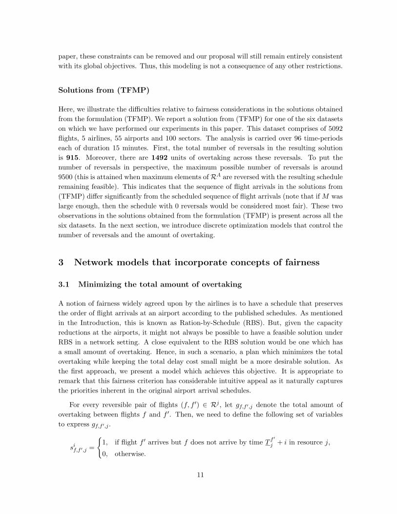
Table 1 summarizes the various feasible combinations of these variables under the abovedefinition. Thus, an alternative way to express sif,f ′,j is as follows:

sif,f ′,j = max{wf′

j,T f ′j +i− wf

j,T f ′j +i

, 0}. (2)

S.No. wfj,T f ′

j +iwf′

j,T f ′j +i

sif,f ′,j

1 0 0 02 0 1 13 1 0 04 1 1 0

Table 1: Truth table for modeling the overtaking variables.

Equation (2) implies that the following constraints suffice to express sif,f ′,j in a mathe-matical programming framework if the objective is to minimize sif,f ′,j :

sif,f ′,j ≥ wf ′

j,T f ′j +i− wf

j,T f ′j +i

, (3a)

sif,f ′,j ≥ 0. (3b)

The set of variables sif,f ′,j are defined for i ∈ {0, . . . , Omaxf,f ′,j}. Now, gf,f ′,j ∈ {0, . . . , Omax

f,f ′,j}can be defined as follows:

gf,f ′,j =

Omaxf,f ′,j∑i=0

sif,f ′,j . (4)

We shall work with an alternative description of Equation (3a) to make the exposition onovertaking clearer. We substitute i = t− T f

′

j in Equation (3a) to rewrite it as follows:

wf′

j,t ≤ wfj,t + s

t−T f ′j

f,f ′,j . (5)

We prove next that the following set of constraints are required to model overtaking between

(f, f ′) ∈ Rj if we use an objective function to minimize gf,f ′,j in addition with st−T f ′

j

f,f ′,j ≥0, ∀t ∈ T reversal

f,f ′,j :

wf′

j,t ≤ wfj,t + s

t−T f ′j

f,f ′,j , ∀t ∈ T reversalf,f ′,j . (6)

12

Theorem 1. If we use an objective function of minimizing gf,f ′,j (the total amount of over-

taking for (f, f ′) ∈ Rj) in addition with st−T f ′

j

f,f ′,j ≥ 0, ∀t ∈ T reversalf,f ′,j , then Constraint (6)

correctly captures the semantics of overtaking.

Proof. In case, there is no reversal, i.e.,

wf′

j,t ≤ wfj,t, ∀t ∈ T

reversalf,f ′,j ,

then Constraint (6) becomes reduntant. Since we minimize total amount of overtaking (and

st−T f ′

j

f,f ′,j ≥ 0, ∀t ∈ T reversalf,f ′,j ), it forces:

st−T f ′

j

f,f ′,j = 0, ∀t ∈ T reversalf,f ′,j ,

leading to gf,f ′,j = 0. On the contrary, if there are i units of overtaking, then ∃t ∈{T f

′

j , . . . , Tf ′

j +Omaxf,f ′,j − i} such that:

wf′

j,t−1 = 0, wf′

j,t = 1,

wfj,t+i−1 = 0, wfj,t+i = 1.

Now, the time-connectivity constraints (Constraints (1f)) imply that:

wf′

j,t+m = 1, wfj,t+m = 0, ∀ 0 ≤ m ≤ i− 1.

Constraint (6) then enforces

skf,f ′,j = 1, ∀ t ≤ k ≤ t+ i− 1.

Again, since we minimize total amount of overtaking (and st−T f ′

j

f,f ′,j ≥ 0, ∀t ∈ T reversalf,f ′,j ), there-

fore,skf,f ′,j = 0, ∀ 0 ≤ k < t, t+ i− 1 < k ≤ Omax

f,f ′,j ,

leading to gf,f ′,j = i. In summary, Constraint (6) (in addition with st−T f ′

j

f,f ′,j ≥ 0), correctlymodel overtaking if the objective function is to minimize gf,f ′,j .

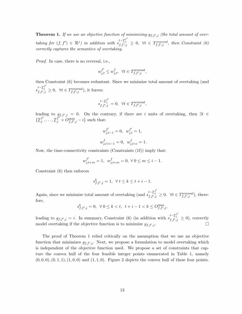
The proof of Theorem 1 relied critically on the assumption that we use an objectivefunction that minimizes gf,f ′,j . Next, we propose a formulation to model overtaking whichis independent of the objective function used. We propose a set of constraints that cap-ture the convex hull of the four feasible integer points enumerated in Table 1, namely(0, 0, 0), (0, 1, 1), (1, 0, 0) and (1, 1, 0). Figure 2 depicts the convex hull of these four points.

13

We introduce the following set of constraints to model overtaking:

wf′

j,t ≤ wfj,t + s

t−T f ′j

f,f ′,j , ∀(f, f ′) ∈ Rj , j ∈ S ∪ K, t ∈ T reversalf,f ′,j . (7a)

wfj,t ≤ wf ′

j,t + 1− st−T f ′

j

f,f ′,j , ∀(f, f ′) ∈ Rj , j ∈ S ∪ K, t ∈ T reversalf,f ′,j . (7b)

wfj,t + st−T f ′

j

f,f ′,j ≤ 1, ∀(f, f ′) ∈ Rj , j ∈ S ∪ K, t ∈ T reversalf,f ′,j . (7c)

−wf′

j,t + st−T f ′

j

f,f ′,j ≤ 0, ∀(f, f ′) ∈ Rj , j ∈ S ∪ K, t ∈ T reversalf,f ′,j . (7d)

PSfrag replacementswfj,t

wf′

j,t

sif,f ′,j

Modeling overtaking

Figure 2: Convex hull of the integer points in Table 1 to model overtaking (i = t− T f′

j ).

The TFMP model with the additional control on total amount of overtaking (referred to asTFMP-Overtake henceforth) is as follows:IZTFMP-Overtake =

min∑f∈F

∑t∈T f

destf

cftotal(t) · (wfdestf ,t

− wfdestf ,t−1)−∑

t∈T forigf

cfg (t) · (wforigf ,t− wforigf ,t−1)

+

λos ·

∑j∈S, (f,f ′)∈Rj

Omaxf,f ′,j∑i=0

sif,f ′,j

+ λoa ·

∑k∈K, (f,f ′)∈Rk

Omaxf,f ′,k∑i=0

sif,f ′,k

subject to:

(1a)− (1g).

(7a)− (7d).

sif,f ′,j ∈ {0, 1}, ∀(f, f ′) ∈ Rj , j ∈ S ∪ K, i ∈ {0, . . . , Omaxf,f ′,j}.

14

3.2 Minimizing the total number of reversals

The model introduced in Section 3.1 took into account the magnitude of overtaking withineach reversal. In this section, we introduce a model which controls the total number ofreversals.

For each element (f, f ′) ∈ Rj , we introduce the following new variable:

sf,f ′,j =

{1, if there is a reversal,

0, otherwise.

Next, we relate the variables sf,f ′,j (used to model a reversal) to the variables sif,f ′,j (usedto model overtaking). It is evident that a reversal occurs if and only if there is at least onetime-period of overtaking. Mathematically, it translates to the following:

sf,f ′,j = 1 ⇐⇒{∃i ∈ {0, . . . , Omax

f,f ′,j}, sif,f ′,j = 1}

(8)

Building upon Equation (8), we have the following:

sf,f ′,j = maxt∈T reversal

f,f ′,j

{st−T f ′

j

f,f ′,j

},

sf,f ′,j = maxt∈T reversal

f,f ′,j

{max{wf

′

j,t − wfj,t, 0}

},

sf,f ′,j = max{

maxt∈T reversal

f,f ′,j

{wf′

j,t − wfj,t}, 0

}. (9)

Equation (9) implies that the following constraints suffice to express sf,f ′,j in a mathematicalprogramming framework if the objective is to minimize sf,f ′,j :

sf,f ′,j ≥ wf′

j,t − wfj,t, ∀t ∈ T

reversalf,f ′,j . (10a)

sf,f ′,j ≥ 0. (10b)

Equation (10a) can be rearranged as follows:

wf′

j,t ≤ wfj,t + sf,f ′,j , ∀t ∈ T reversal

f,f ′,j . (11)

Theorem 2. If we use an objective function of minimizing sf,f ′,j, then Constraint (11) inaddition with sf,f ′,j ≥ 0 correctly captures the semantics of modeling a reversal.

Proof. In case, there is no reversal, i.e.,

wf′

j,t ≤ wfj,t, ∀t ∈ T

reversalf,f ′,j ,

then Constraint (11) becomes redundant. Since we minimize sf,f ′,j (and sf,f ′,j ≥ 0), it forcessf,f ′,j = 0. On the contrary, if there is a reversal, then ∃t ∈ T reversal

f,f ′,j such that:

wf′

j,t = 1, wfj,t = 0.

Constraint (11) then implies that sf,f ′,j ≥ 1. Again, minimizing sf,f ′,j makes sf,f ′,j = 1ensuring that Constraint (11) indeed models a reversal correctly.

15

The proof of Theorem 2 relied critically on the assumption that we use an objective func-tion that minimizes sf,f ′,j . Here, we present a formulation that models a reversal correctlyindependently of the objective function used. For each element (f, f ′) ∈ Rj , we introducethe following constraints to (TFMP):

wf′

j,t ≤ wfj,t + sf,f ′,j , ∀(f, f ′) ∈ Rj , j ∈ S ∪ K, t ∈ T reversal

f,f ′,j . (12a)

wfj,t ≤ wf ′

j,t + 1− sf,f ′,j , ∀(f, f ′) ∈ Rj , j ∈ S ∪ K, t ∈ T reversalf,f ′,j . (12b)

If there is a reversal between flights f and f ′ in resource j, i.e., sf,f ′,j = 1, then Constraint(12a) becomes redundant and Constraint (12b) stipulates that if flight f has arrived by timet, then flight f ′ has to arrive by that time, hence ensuring that flight f cannot arrive beforeflight f ′. Similarly, if there is no reversal, i.e., sf,f ′,j = 0, then Constraint (12b) becomesredundant and Constraint (12a) stipulates that if flight f ′ has arrived by time t, then flight fhas to arrive by that time, hence ensuring that flight f ′ cannot arrive before flight f . Thus,we are able to model a reversal with the addition of only one variable (sf,f ′,j).

Given this additional set of constraints, the model then minimizes a weighted combi-nation of total delay costs and total number of reversals. The parameters λrs and λra arechosen appropriately to control the degree of fairness in sector reversals and airport reversalsrespectively.

(TFMP) extended with reversals: (TFMP-Reversal).

The TFMP model with the additional control on reversals is as follows:IZTFMP-Reversal =

min∑f∈F

∑t∈T f

destf

cftotal(t) · (wfdestf ,t

− wfdestf ,t−1)−∑

t∈T forigf

cfg (t) · (wforigf ,t− wforigf ,t−1)

+

λrs ·

∑j∈S, (f,f ′)∈Rj

sf,f ′,j

+ λra ·

∑k∈K, (f,f ′)∈Rk

sf,f ′,k

subject to:

(1a)− (1g).

(12a)− (12b).

sf,f ′,j ∈ {0, 1}, ∀(f, f ′) ∈ Rj , j ∈ S ∪ K.

For each element (f, f ′) ∈ Rj , let IPReversal(f, f ′, j) denote the set of all feasible binaryvectors satisfying Constraints (12a) and (12b). We show in the Appendix that the polyhedron

16

induced by Constraints (12a) and (12b) is the convex hull of solutions in IPReversal(f, f ′, j).

IPReversal(f, f ′, j) ={wfj,t ∈ {0, 1}, sf,f ′,j ∈ {0, 1}|

wf′

j,t − wfj,t − sf,f ′,j ≤ 0, t ∈ T reversal

f,f ′,j ,

wfj,t − wf ′

j,t + sf,f ′,j ≤ 1, t ∈ T reversalf,f ′,j .

}Remark 2. RBS Policy - a special case of (TFMP-Reversal). When there is sufficientcapacity at all airports, such that a feasible solution under RBS exists (i.e., there are noreversals), this model is capable of generating that solution (using a sufficiently high λra)while minimizing the total delay costs. Hence, a solution under RBS policy is a special caseof our model. Since, a solution under RBS preserves the order of flight arrivals, therefore,for every pair of flights (f, f ′) ∈ RA, the variable sf,f ′,destf

= 0, and Constraints (12a) and(12b) reduce to Constraint (13) which ensures that flight f ′ cannot arrive before flight f :

wf′

destf ′ ,t≤ wfdestf ,t

, ∀(f, f ′) ∈ RA, t ∈ T reversalf,f ′,destf

. (13)

3.3 Prioritizing between airport reversals and sector reversals

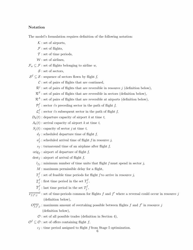
In Section 3.2, we introduced a discrete optimization model with the capability of controllingsector reversals in addition to airport reversals. In this section, we discuss the relative meritsof controlling sector reversals. In Section 6.6, we report empirical evidence to validate ourconclusions.

To start with, it seems reasonable to expect that primary stakeholders (airlines andflying passengers) won’t be bothered as to how the en-route resources are allocated if theyare satisfied with the final outcome of the arrival sequences at the airports. In fact, thisscheme of things would be acceptable to the FAA as its key objective in designing variousATFM programs is to satisfy these primary stakeholders. In addition to this observation, wefeel there are two key arguments in favor of controlling sector reversals:

1. AFPs. The first pertains to the operational details of AFPs (one of the recent ATFMprograms) under the current CDM practice. The recently introduced AFPs operatemuch like GDPs, i.e., the arrival slots in the affected airspace are allotted using theRBS principle. Therefore, in a scenario where multiple AFPs and GDPs operate si-multaneously, a natural extension of fairness is controlling reversals in the en-routeairspace affected by an AFP. To elaborate, we give the following example:

Example 3.1. Consider the scenario depicted in Figure 3. There is an AFP operationalin the en-route airspace followed by a GDP at BOS (Boston). Simultaneously, thereis another airport LGA (New York LaGuardia) nearby with no GDP. There are twostreams of flights going through the AFP to one of these airports. In a scenario wheresector reversals in the AFP are not controlled, a schedule with no airport reversals mightbe such that all flights going to BOS are allowed to go first before any other flight to

17

LGA through the AFP. Such a plan might not be acceptable to the stakeholders of LGAbecause all flights destined to LGA are assigned large delays even though they are partof an ATFM program (the AFP in this case). This might get further exacerbated in ascenario where LGA (the non-GDP airport) is a hub airport for a particular airline, inwhich case this airline is clearly not treated equitably.

2. Stochastic capacities. The second argument is a result of a stochastic setting,wherein the future realized capacity can be quite different compared to the deter-ministic capacity inputs used in the optimization model. In this scenario, it is possiblethat controlling sector reversals might lead to a schedule which is able to mitigate theimpacts caused due to stochastic nature of future capacities.

PSfrag replacementsBOS (GDP)

LGA (No GDP)

AFP

Figure 3: Illustration of a scenario where controlling sector reversals seems appropriate.There are multiple ATFM programs operating simultaneously. Specifically, an AFP is spa-tially followed by an airport with a GDP (BOS) and an airport with no GDP (LGA).

On the negative side, we believe that imposing additional constraints of controlling sectorreversals will lead to two key impacts: i) increase in system delays over a solution which onlycontrols airport reversals; and ii) potential change in the number of airport reversals (due todownstream effects). Thus, in this balancing act, these two consequences have to be carefullymitigated to ensure neither one gets exacerbated.

In summary, the discussion in this section culminates with the conclusion that control-ling sector reversals should be a secondary goal. Consequently, we propose that in the modelTFMP-Reversal, the tradeoff parameter λrs used to control sector reversals be set to a sig-nificantly lower value as compared to the parameter λra used to control airport reversals.

Extensions. We now elaborate on how the proposed models (TFMP-Reversal and TFMP-Overtake) can be extended to accommodate alternative objective functions.

• Incorporating alternative objective functions:Although the models presented in this paper minimize the number of reversals andamount of overtaking, it is possible to extend them to accommodate alternative objec-tive functions. For instance, suppose we want to equalize the resulting reversals andovertaking among airlines taking into account the number of flights they operate. Thiscan be achieved as follows:Let dw denote the number of reversals per flight for airline w and γ denote the mean

18

of the dw’s across all airlines.

dw =

( ∑f ′∈Fw

sf,f ′

)/|Fw|,

γ =

( ∑w∈W

dw

)/|W|.

Then, we add∣∣dw−γ∣∣ term to the objective function of minimizing the total delay cost

with an appropriate tradeoff parameter.

Size of the Formulations. Denoting with

N = maxf∈F|Sf |,

the total number of decision variables and constraints for the various models can be boundedas listed in Table 2.

Model No. of Decision No. ofVariables Constraints

TFMP |F|MN 2|K||T |+ |S||T |+ 2|F|MN + 2|F|N +M |C|TFMP-Reversal |F|MN + |RA| 2|K||T |+ |S||T |+ 2|F|MN + 2|F|M +M |C|+ 2|RA|MTFMP-Overtake |F|MN +M |RA| 2|K||T |+ |S||T |+ 2|F|MN + 2|F|N +M |C|+ |RA|M

Table 2: Upper bound on the size of the models.

In order to get a feeling of the size of the formulations, let us consider an example thatadequately represents the U.S. network.

Example 3.2. Let |K| = 50, |T | = 100, |S| = 100, |RA| = 50000, |F| = 10000, |C| = 8000,M = 6 and N = 5. The duration of each period is 15 minutes implying a planning horizon ofalmost a day. For this example, the upper bound on the number of variables and constraintsare listed in Table 3.

Model No. of Decision No. ofVariables Constraints

TFMP 300,000 780,000TFMP-Reversal 350,000 1,380,000TFMP-Overtake 600,000 1,080,000

Table 3: Numerical Example: Upper bound on the size of the models.

Since we introduce only one class of variables sf,f ′,j for all elements (f, f ′) ∈ Rj , thenumber of variables in the model (TFMP-Reversal) are comparable to the original model(TFMP).

19

4 Network model for slot reallocation that incorporates air-

line collaboration

In this section, we present a model (called TFMP-Trading) for slot reallocation in a networksetting that introduces only one additional variable per offer above the TFMP model. Welet airlines submit offers to trade slots assigned to its flights across different airports. Theexecuted set of trades should ensure that the resulting schedule is still feasible taking intoaccount all kinds of network connectivities and airspace capacities.

The set O (Set of Airline Offers)

We give next the definition of O (set of airline offers). We use a structure proposed by Vossenand Ball [19] that allows the airlines to submit so-called “at-least, at-most” offers. Airlinessubmit offers of the following kind: (fd, td′ ; fu, tu′) which means that the airline is willing tomove flight fd to a later time-period, but no later than td′ ; in return for moving flight fu toan earlier time-period, but no later than tu′ . The destination airports of flights fd and fuare allowed to be distinct. Figure 4 gives an example to illustrate the semantics of the offerstructure. The set O contains all such four-tuples (fd, td′ ; fu, tu′) submitted by the airlinesafter a schedule is generated from Stage I of our proposal. Note that cfd

and cfu denote theslots allotted to the two flights from Stage I, and hence, for such an offer to be useful, wemust have cfd

< td′ and cfu > tu′ . Finally, Of ⊆ O defines the set of offers containing flightf .

PSfrag replacementscfd

td′

tu′

cfu

Airport AAirport B

Figure 4: Illustration of the structure of an offer (fd, td′ ; fu, tu′). destfd= A, destfu = B,

td′ = cfd+ 3 and tu′ = cfu − 4. The offer states that the airline is willing to delay flight fd

by at-most 3 slots if in return flight fu is moved earlier by at-least 4 slots.

4.1 (TFMP-Trading): A model for slot reallocation in a network setting

Here, we introduce our model of slot reallocation in a network setting. The model onlyintroduces one additional variable per offer in addition to wfj,t, which are the variables used

20

in the TFMP model of Bertsimas Stock-Patterson [5].

The Decision Variables

• odd′uu′ ∈ {0, 1} = 1 if offer (fd, td′ ; fu, tu′) is executed.

Constraints

(1a)− (1g).

odd′uu′ ≤ wfddestfd

,td′, ∀(fd, td′ ; fu, tu′) ∈ O. (14a)

odd′uu′ ≤ wfu

destfu ,tu′, ∀(fd, td′ ; fu, tu′) ∈ O. (14b)∑

j∈Of

oj ≤ 1, ∀f ∈ F . (14c)

wfdestf ,cf− wfdestf ,cf−1 ≥ 1− (

∑j∈Of

oj), ∀f ∈ F . (14d)

wfj,t ∈ {0, 1}, ∀f ∈ F , j ∈ Sf , t ∈ T fj . (14e)

odd′uu′ ∈ {0, 1}, ∀(fd, td′ ; fu, tu′) ∈ O. (14f)

Constraints (14a) and (14b) enforce that when an offer odd′uu′ is executed (i.e., odd′uu′ = 1),then wfd

destfd,td′

= 1 and wfu

destfu ,tu′= 1, i.e., flights fd and fu cannot arrive after the respective

time-periods in the offer, namely, t′d and t′u. This ensures that the semantics of the structureof an offer are satisfied. Constraint (14c) enforces that for each flight, at most one offer canget executed. Moreover, constraint (14d) stipulates that if no offer for a flight f is executed(i.e., oj = 0, ∀j ∈ Of ), then the flight will arrive at the time-period allotted from Stage I(cf ).

Objective Function

In the model presented above, we have not explicitly stated the objective function that shouldbe used. It is evident that fairness in the number of executed offers across airlines wouldagain be relevant in this stage of our proposal.

Let nw denote the number of trades executed corresponding to airline w, and let γ denotethe mean of the trades executed across all airlines.

nw =∑

f∈Fw,j∈Of

oj ,

γ =( ∑w∈W

nw

)/|W|.

21

In the next section, we report computational results based on the following two objectivefunctions:

• Objective 1 : maximize the total number of trades (max∑

(fd,td′ ;fu,tu′ )∈Oodd′uu′).

• Objective 2 : minimize the difference in the number of trades executed for each airlinefrom the mean (min

∑w∈W |nw − γ|).

5 Integration and comparison with current CDM practice

Given that our aspiration in this research effort is to bridge the gap between theory andpractice, we now elaborate on how our proposal can be integrated within the broader CDMparadigm currently in use. Our goal in this section is to demonstrate the practical viabilityof our procedural framework and verify the compatibility of the input and output datarequirements of our models with the available operational technology.

We start by revisiting the CDM paradigm alluded to in the Introduction and provide adetailed description of the phases involved in the coordination of various ATFM initiatives(like GDPs and AFPs). There are three key phases involved in the decision-making process:

1. RBS for each ATFM program. FAA invokes the RBS policy to allocate arrivalslots to the airlines for each ATFM program based on the original schedule ordering.

2. Airline response to schedule disruption. Based on the slots allotted, an airlineis allowed to make changes to the schedule by canceling flights and swapping the slotsof two or more of its own flights if they are compatible with the scheduled departuretimes.

3. Final coordination by the FAA. FAA accepts the relevant changes proposed by theairlines to come up with a overall feasible schedule. This is further complemented byCompression (wherein the FAA attempts to fill in any holes created by cancellationsto further optimize the final schedule).

We now demonstrate how our proposal can be integrated within the three-stage CDMframework described above. To start with, we propose to filter in the flights affected byall ATFM programs that the FAA intends to use. The trajectories of all other flights aredeterministically fixed and the capacity corresponding to them is removed from the capacityinputs to our optimization models.

• Stage 1: Control reversals/overtaking. This stage of our proposal interfaces withphase 1 of the CDM framework. Rather than applying RBS to each ATFM program, wecontrol the reversals and overtaking in the resulting flight sequences by using TFMP-Reversal and TFMP-Overtake. The input requirements for our models, namely, the

22

set of feasible times that a flight can be in a sector and the capacity inputs are readilyavailable from Flight Schedule Monitor (FSM)1. Furthermore, the output of our modelscan be easily converted to a slot assignment for each flight (by following the scheduledorder of the slots allotted for flights during each time-period) and thus is compatiblewith the current operational practice.

• Stage 2: Airline collaboration. This stage of our proposal interfaces with thelast two phases of the CDM framework. The input required from the airlines on theoffers to trade are readily available as the airlines know the slots allotted to themfrom Stage 1. Moreover, airlines also propose flights cancellations (emanating fromoperational infeasibility) after considering their slot assignments. The final exercise ofCompression goes through as is done presently to fill in gaps.

These two stages can be repeated (if necessary) to enable program revisions. In summary, webelieve that our proposal fits well within the CDM framework used currently and the datainput and output requirements are compatible with operational feasibility.

6 Computational Results

In this section, we report computational results from the optimization models introduced inSection 3 and Section 4 on national-scale, real world datasets spanning across six days. Thedataset for each day encompasses 55 major airports of the US and covers operations of thetop five airlines. Each dataset contains data on the actual flight arrival and departure timesfor that particular day which lets us compute the actual delays.

6.1 Statistics of the Datasets

Table 4 summarizes the statistics of six days of flights data. These correspond to the op-erations at the 55 major airports of the US. We filter in the flights corresponding to theoperations of the top 5 airlines (measured by the number of flight operations) - Southwest(SWA), American (AAL), Delta (DAL), United (UAL) and Northwest (NWA) to enable usto better analyze the results.

6.2 Experimental Setup

In our experimental setup, the airspace is subdivided into sectors of equal dimensions (10 by10) that form a grid, thereby, having a total of 100 sectors. The 55 major airports of the

1FSM is an important software technology currently used by FAA that provides users with up-to-date,

real-time information on the future flight behavior and provides common system-wide situational awareness

for all stakeholders

23

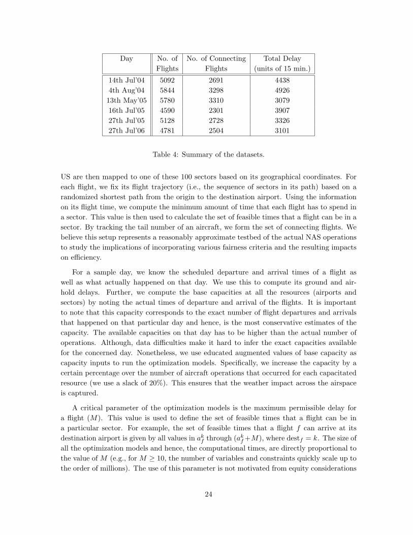
Day No. of No. of Connecting Total DelayFlights Flights (units of 15 min.)

14th Jul’04 5092 2691 44384th Aug’04 5844 3298 4926

13th May’05 5780 3310 307916th Jul’05 4590 2301 390727th Jul’05 5128 2728 332627th Jul’06 4781 2504 3101

Table 4: Summary of the datasets.

US are then mapped to one of these 100 sectors based on its geographical coordinates. Foreach flight, we fix its flight trajectory (i.e., the sequence of sectors in its path) based on arandomized shortest path from the origin to the destination airport. Using the informationon its flight time, we compute the minimum amount of time that each flight has to spend ina sector. This value is then used to calculate the set of feasible times that a flight can be in asector. By tracking the tail number of an aircraft, we form the set of connecting flights. Webelieve this setup represents a reasonably approximate testbed of the actual NAS operationsto study the implications of incorporating various fairness criteria and the resulting impactson efficiency.

For a sample day, we know the scheduled departure and arrival times of a flight aswell as what actually happened on that day. We use this to compute its ground and air-hold delays. Further, we compute the base capacities at all the resources (airports andsectors) by noting the actual times of departure and arrival of the flights. It is importantto note that this capacity corresponds to the exact number of flight departures and arrivalsthat happened on that particular day and hence, is the most conservative estimates of thecapacity. The available capacities on that day has to be higher than the actual number ofoperations. Although, data difficulties make it hard to infer the exact capacities availablefor the concerned day. Nonetheless, we use educated augmented values of base capacity ascapacity inputs to run the optimization models. Specifically, we increase the capacity by acertain percentage over the number of aircraft operations that occurred for each capacitatedresource (we use a slack of 20%). This ensures that the weather impact across the airspaceis captured.

A critical parameter of the optimization models is the maximum permissible delay fora flight (M). This value is used to define the set of feasible times that a flight can be ina particular sector. For example, the set of feasible times that a flight f can arrive at itsdestination airport is given by all values in akf through (akf +M), where destf = k. The size ofall the optimization models and hence, the computational times, are directly proportional tothe value of M (e.g., for M ≥ 10, the number of variables and constraints quickly scale up tothe order of millions). The use of this parameter is not motivated from equity considerations

24

and has no consequences on the fairness properties of the resulting schedules. We use a valueof M = 6, which corresponds to 6 time periods (each of length 15 minutes), hence permittinga maximum delay of 90 minutes.

Remark 3. While a small value of M will facilitate the computational efficiency of the op-timization models, the framework is generic enough to allow for a larger value of M for aselect set of flights for which higher delays are expected (or desired).

To compute optimal solutions, we use the CPLEX-MIP solver 11.0, implemented usingAMPL as a modeling language on a laptop with 2 GB RAM and Linux Ubuntu OS. Theinstances reported in this paper have a typical size of the order of 300,000 variables (this in-creases significantly for TFMP-Overtake) and 800,000 constraints (this increases significantlyfor TFMP-Reversal).

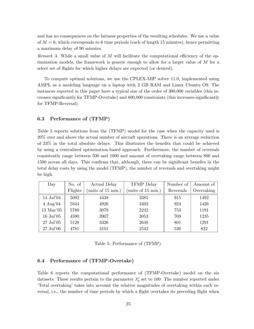
6.3 Performance of (TFMP)

Table 5 reports solutions from the (TFMP) model for the case when the capacity used is20% over and above the actual number of aircraft operations. There is an average reductionof 23% in the total absolute delays. This illustrates the benefits that could be achievedby using a centralized optimization-based approach. Furthermore, the number of reversalsconsistently range between 500 and 1000 and amount of overtaking range between 800 and1500 across all days. This confirms that, although, there can be significant benefits in thetotal delay costs by using the model (TFMP), the number of reversals and overtaking mightbe high.

Day No. of Actual Delay TFMP Delay Number of Amount ofFlights (units of 15 min.) (units of 15 min.) Reversals Overtaking

14 Jul’04 5092 4438 3385 915 14924 Aug’04 5844 4926 3492 924 1426

13 May’05 5780 3079 2242 753 119116 Jul’05 4590 3907 3053 769 123527 Jul’05 5128 3326 2648 801 129127 Jul’06 4781 3101 2542 526 822

Table 5: Performance of (TFMP).

6.4 Performance of (TFMP-Overtake)

Table 6 reports the computational performance of (TFMP-Overtake) model on the sixdatasets. These results pertain to the parameter λoa set to 100. The number reported under‘Total overtaking’ takes into account the relative magnitudes of overtaking within each re-versal, i.e., the number of time periods by which a flight overtakes its preceding flight when

25

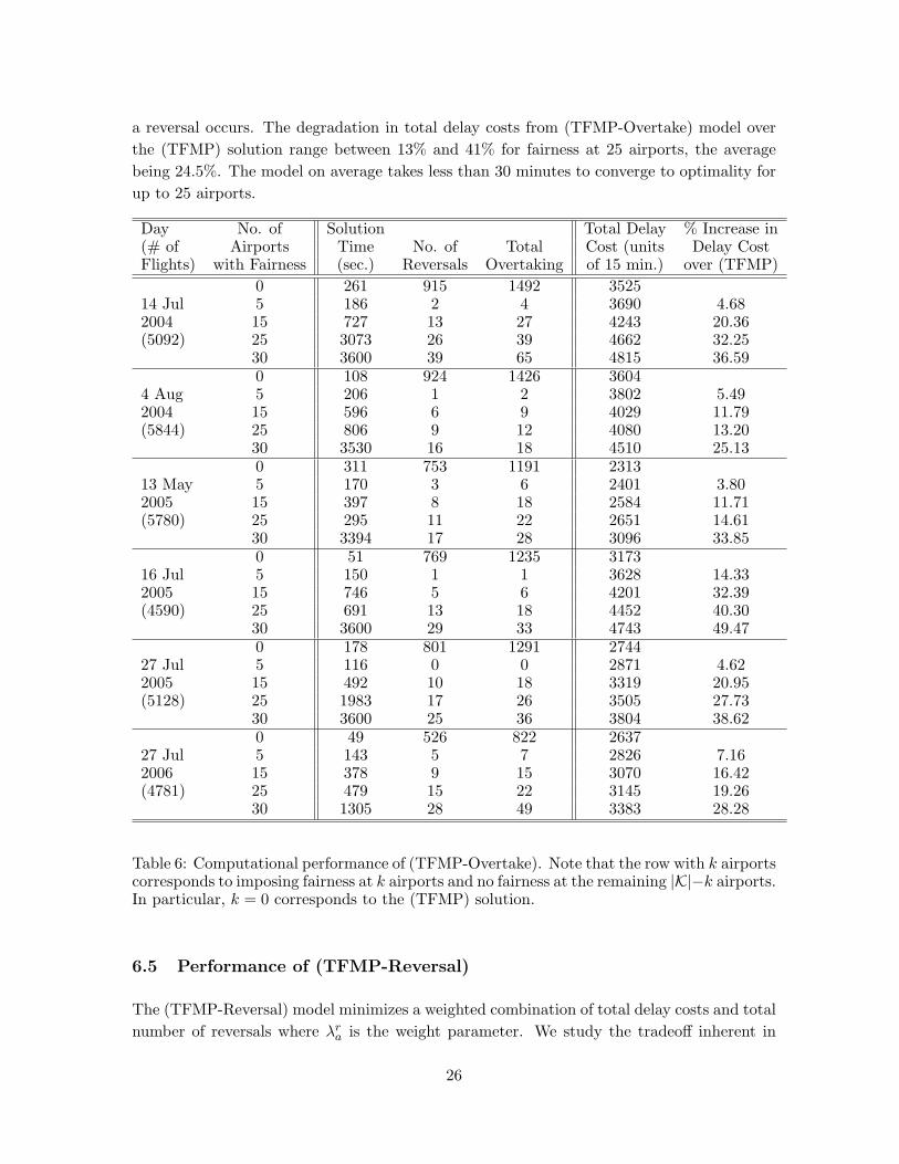
a reversal occurs. The degradation in total delay costs from (TFMP-Overtake) model overthe (TFMP) solution range between 13% and 41% for fairness at 25 airports, the averagebeing 24.5%. The model on average takes less than 30 minutes to converge to optimality forup to 25 airports.

Day No. of Solution Total Delay % Increase in(# of Airports Time No. of Total Cost (units Delay CostFlights) with Fairness (sec.) Reversals Overtaking of 15 min.) over (TFMP)

0 261 915 1492 352514 Jul 5 186 2 4 3690 4.682004 15 727 13 27 4243 20.36(5092) 25 3073 26 39 4662 32.25

30 3600 39 65 4815 36.590 108 924 1426 3604

4 Aug 5 206 1 2 3802 5.492004 15 596 6 9 4029 11.79(5844) 25 806 9 12 4080 13.20

30 3530 16 18 4510 25.130 311 753 1191 2313

13 May 5 170 3 6 2401 3.802005 15 397 8 18 2584 11.71(5780) 25 295 11 22 2651 14.61

30 3394 17 28 3096 33.850 51 769 1235 3173

16 Jul 5 150 1 1 3628 14.332005 15 746 5 6 4201 32.39(4590) 25 691 13 18 4452 40.30

30 3600 29 33 4743 49.470 178 801 1291 2744

27 Jul 5 116 0 0 2871 4.622005 15 492 10 18 3319 20.95(5128) 25 1983 17 26 3505 27.73

30 3600 25 36 3804 38.620 49 526 822 2637

27 Jul 5 143 5 7 2826 7.162006 15 378 9 15 3070 16.42(4781) 25 479 15 22 3145 19.26

30 1305 28 49 3383 28.28

Table 6: Computational performance of (TFMP-Overtake). Note that the row with k airportscorresponds to imposing fairness at k airports and no fairness at the remaining |K|−k airports.In particular, k = 0 corresponds to the (TFMP) solution.

6.5 Performance of (TFMP-Reversal)

The (TFMP-Reversal) model minimizes a weighted combination of total delay costs and totalnumber of reversals where λra is the weight parameter. We study the tradeoff inherent in

26

these conflicting objectives in two ways - a) as a function of the tradeoff parameter λra andb) as a function of the number of airports where this fairness criterion is imposed.

The effect of the tradeoff parameter

Figure 5 plots the tradeoff in the number of reversals with the total delay cost as a functionof λra for fairness based on controlling total reversals imposed at 25 airports. The five pointson the plot for each day correspond to the result from (TFMP-Reversal) with λra = 0, 1, 10,100 and 1000. Initially, there is a significant reduction in the number of reversals at the costof a small increase in total delay cost, but the subsequent benefits in the number of reversalscome at a high cost. For all days, the model is able to achieve less than 100 reversals for adegradation of at most 10% in the total delay cost. To achieve reversals between 10 and 30,the degradation in total delay costs range between 10% and 40% across all days.

PSfrag replacements

% Increase in total delay cost over TFMP

Total number of airport reversals

Tradeoff between airport reversals and total delay cost

14 Jul’04

4 Aug’04

13 May’05

16 Jul’05

27 Jul’05

27 Jul’06

Figure 5: Effect of the tradeoff parameter λra. The five points for each day correspond to the

result from (TFMP-Reversal) with λra = 0, 1, 10, 100 and 1000.

The effect of the number of airports

Table 7 reports the computational performance of the (TFMP-Reversal) model on the sixdatasets as a function of the number of airports where this fairness criterion is imposed. Theseresults pertain to the tradeoff parameter λra set to 100. As is evident from the results reportedacross all days, the number of reversals can be controlled up to 10-30. The degradation intotal delay costs from (TFMP-Reversal) model over the (TFMP) solution range between

27

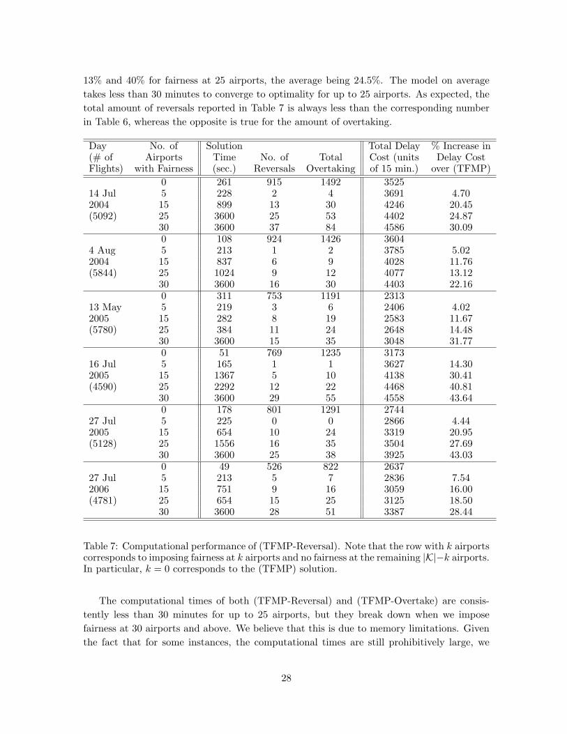
13% and 40% for fairness at 25 airports, the average being 24.5%. The model on averagetakes less than 30 minutes to converge to optimality for up to 25 airports. As expected, thetotal amount of reversals reported in Table 7 is always less than the corresponding numberin Table 6, whereas the opposite is true for the amount of overtaking.

Day No. of Solution Total Delay % Increase in(# of Airports Time No. of Total Cost (units Delay CostFlights) with Fairness (sec.) Reversals Overtaking of 15 min.) over (TFMP)

0 261 915 1492 352514 Jul 5 228 2 4 3691 4.702004 15 899 13 30 4246 20.45(5092) 25 3600 25 53 4402 24.87

30 3600 37 84 4586 30.090 108 924 1426 3604

4 Aug 5 213 1 2 3785 5.022004 15 837 6 9 4028 11.76(5844) 25 1024 9 12 4077 13.12

30 3600 16 30 4403 22.160 311 753 1191 2313

13 May 5 219 3 6 2406 4.022005 15 282 8 19 2583 11.67(5780) 25 384 11 24 2648 14.48

30 3600 15 35 3048 31.770 51 769 1235 3173

16 Jul 5 165 1 1 3627 14.302005 15 1367 5 10 4138 30.41(4590) 25 2292 12 22 4468 40.81

30 3600 29 55 4558 43.640 178 801 1291 2744

27 Jul 5 225 0 0 2866 4.442005 15 654 10 24 3319 20.95(5128) 25 1556 16 35 3504 27.69

30 3600 25 38 3925 43.030 49 526 822 2637

27 Jul 5 213 5 7 2836 7.542006 15 751 9 16 3059 16.00(4781) 25 654 15 25 3125 18.50

30 3600 28 51 3387 28.44

Table 7: Computational performance of (TFMP-Reversal). Note that the row with k airportscorresponds to imposing fairness at k airports and no fairness at the remaining |K|−k airports.In particular, k = 0 corresponds to the (TFMP) solution.

The computational times of both (TFMP-Reversal) and (TFMP-Overtake) are consis-tently less than 30 minutes for up to 25 airports, but they break down when we imposefairness at 30 airports and above. We believe that this is due to memory limitations. Giventhe fact that for some instances, the computational times are still prohibitively large, we

28

study the times needed to achieve a solution that is within 20% of the optimal. In all cases,we could achieve feasible solutions satisfying this optimality criterion in less than 15 minutes.

6.6 Controlling sector reversals and balancing with airport reversals

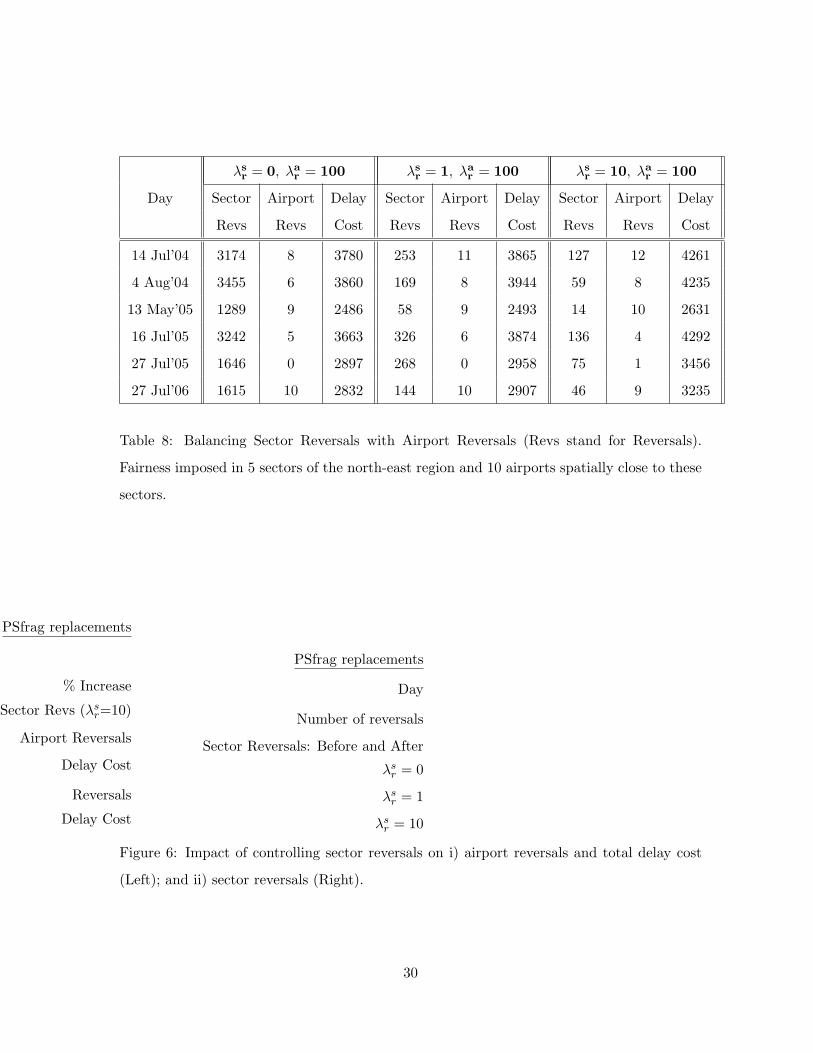
As concluded in Section 3, we believe that controlling airport reversals (and overtaking) isour primary objective, and controlling sector reversals represents a secondary goal. In thissection, we study the interaction of the two objectives with the aim to quantify the priceof controlling sector reversals (on airport reversals and total delay cost). Our setup for thisexercise comprises of controlling reversals in 5 sectors of the north-east region of the US anda set of 10 airports that lie spatially close to these sectors (we believe this would be thetypical setting with multiple AFPs and GDPs operating simultaneously). Table 8 reportsthe sector reversals, airport reversals and total delay cost for different combinations of thetradeoff parameters λsr and λar .

The left plot in Figure 6 is a box plot quantifying the percentage increase in the numberof airport reversals and the delay cost by enforcing the additional control on sector reversalsfor the tradeoff parameter λsr = 10. The percentage increase in delay cost lies between 5%and 20% with a mean of around 13%, whereas the percentage increase in airport reversalsis around 5%. Moreover, the sector reversals can be reduced from the order of 1000s to 10s.In contrast, for λsr = 1, the average increase in the total delay cost is 3% on average butthe sector reversals are still in the 100s. The right plot in Figure 6 depicts the reductionin number of sector reversals possible by this explicit control (potential reduction from fourdigit reversals to two digit reversals).

Consequently, our overall conclusion regarding control of sector reversals is as follows:

1. We have developed a model capable of controlling sector reversals in conjunction withairport reversals.

2. We believe controlling sector reversals is a secondary goal after achieving the primaryobjective of controlling airport reversals. This is validated by our computational exper-iments of the form presented here (the impact on total delay cost is substantial (13% onaverage) for large λsr (=10) and is relatively small (3% on average) for small λsr (=1)).

6.7 Interaction with super-linear cost coefficients

We used super-linear cost coefficients in the overall objective function as additional means toimpose equity. As explained earlier in Section 2, this eliminates flights with extreme delays.Since, our primary fairness proposal is controlling reversals and overtaking, we study theinteraction of super-linear cost coefficients with this fairness criteria.

29

λsr = 0, λa

r = 100 λsr = 1, λa

r = 100 λsr = 10, λa

r = 100

Day Sector Airport Delay Sector Airport Delay Sector Airport Delay

Revs Revs Cost Revs Revs Cost Revs Revs Cost

14 Jul’04 3174 8 3780 253 11 3865 127 12 4261

4 Aug’04 3455 6 3860 169 8 3944 59 8 4235

13 May’05 1289 9 2486 58 9 2493 14 10 2631

16 Jul’05 3242 5 3663 326 6 3874 136 4 4292

27 Jul’05 1646 0 2897 268 0 2958 75 1 3456

27 Jul’06 1615 10 2832 144 10 2907 46 9 3235

Table 8: Balancing Sector Reversals with Airport Reversals (Revs stand for Reversals).

Fairness imposed in 5 sectors of the north-east region and 10 airports spatially close to these

sectors.

PSfrag replacements

% Increase

Box Plot: Impact of Sector Revs (λsr=10)

Airport Reversals

Delay Cost

Reversals

Delay Cost

PSfrag replacements

Day

Number of reversals

Sector Reversals: Before and After

λsr = 0

λsr = 1

λsr = 10

Figure 6: Impact of controlling sector reversals on i) airport reversals and total delay cost

(Left); and ii) sector reversals (Right).

30

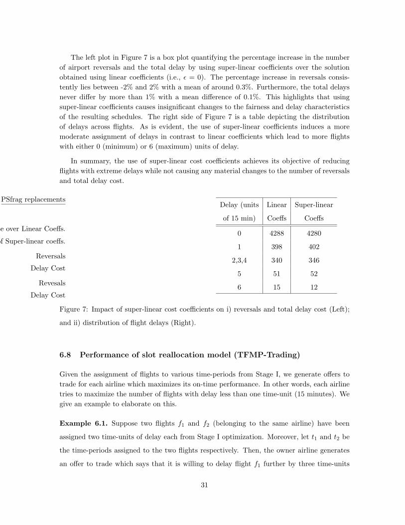
The left plot in Figure 7 is a box plot quantifying the percentage increase in the numberof airport reversals and the total delay by using super-linear coefficients over the solutionobtained using linear coefficients (i.e., ε = 0). The percentage increase in reversals consis-tently lies between -2% and 2% with a mean of around 0.3%. Furthermore, the total delaysnever differ by more than 1% with a mean difference of 0.1%. This highlights that usingsuper-linear coefficients causes insignificant changes to the fairness and delay characteristicsof the resulting schedules. The right side of Figure 7 is a table depicting the distributionof delays across flights. As is evident, the use of super-linear coefficients induces a moremoderate assignment of delays in contrast to linear coefficients which lead to more flightswith either 0 (minimum) or 6 (maximum) units of delay.

In summary, the use of super-linear cost coefficients achieves its objective of reducingflights with extreme delays while not causing any material changes to the number of reversalsand total delay cost.

PSfrag replacements

% Increase over Linear Coeffs.

Box Plot: Impact of Super-linear coeffs.

Reversals

Delay Cost

Revesals

Delay Cost

Delay (units Linear Super-linear

of 15 min) Coeffs Coeffs

0 4288 4280

1 398 402

2,3,4 340 346

5 51 52

6 15 12

Figure 7: Impact of super-linear cost coefficients on i) reversals and total delay cost (Left);

and ii) distribution of flight delays (Right).

6.8 Performance of slot reallocation model (TFMP-Trading)

Given the assignment of flights to various time-periods from Stage I, we generate offers totrade for each airline which maximizes its on-time performance. In other words, each airlinetries to maximize the number of flights with delay less than one time-unit (15 minutes). Wegive an example to elaborate on this.

Example 6.1. Suppose two flights f1 and f2 (belonging to the same airline) have been

assigned two time-units of delay each from Stage I optimization. Moreover, let t1 and t2 be

the time-periods assigned to the two flights respectively. Then, the owner airline generates

an offer to trade which says that it is willing to delay flight f1 further by three time-units

31

if in return flight f2 can arrive within one time-unit of delay, i.e., it generates the offer

(f1, t1 + 3; f2, t2− 1). Thus, in case, this trade is executed, then flight f2 will arrive on-time,

thereby improving the internal objective function of the airline (which is to maximize the

on-time performance).

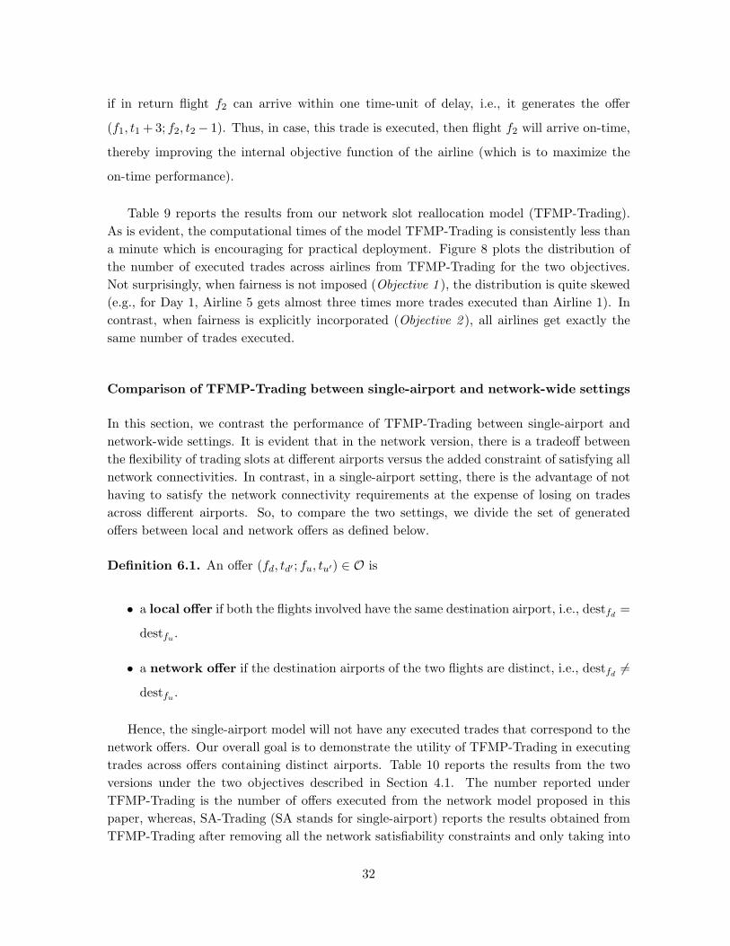
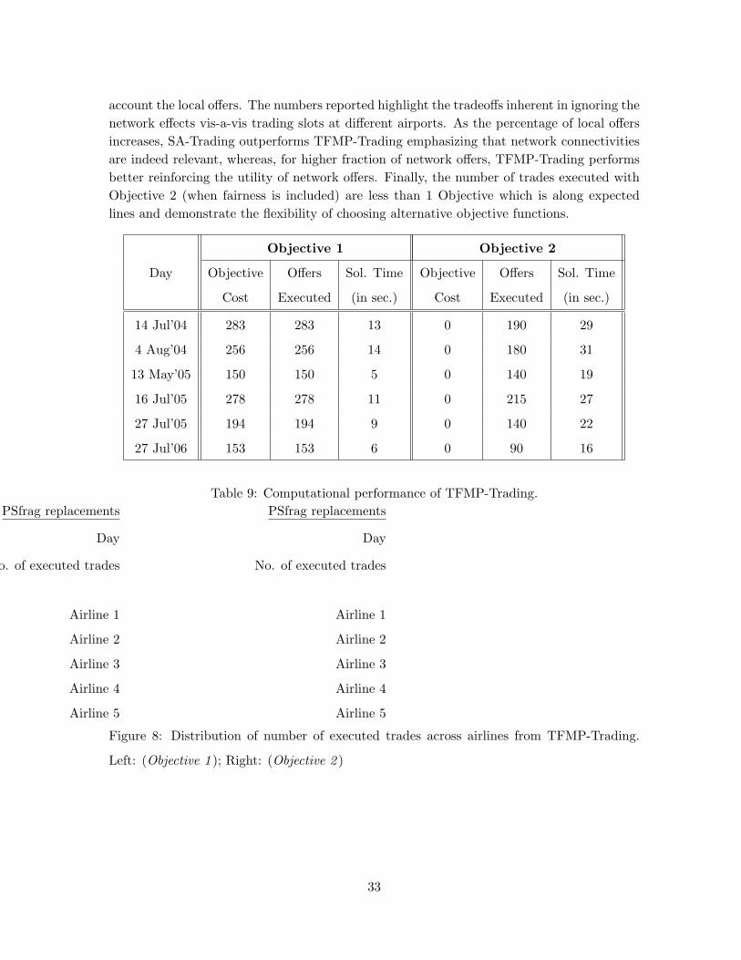
Table 9 reports the results from our network slot reallocation model (TFMP-Trading).As is evident, the computational times of the model TFMP-Trading is consistently less thana minute which is encouraging for practical deployment. Figure 8 plots the distribution ofthe number of executed trades across airlines from TFMP-Trading for the two objectives.Not surprisingly, when fairness is not imposed (Objective 1 ), the distribution is quite skewed(e.g., for Day 1, Airline 5 gets almost three times more trades executed than Airline 1). Incontrast, when fairness is explicitly incorporated (Objective 2 ), all airlines get exactly thesame number of trades executed.

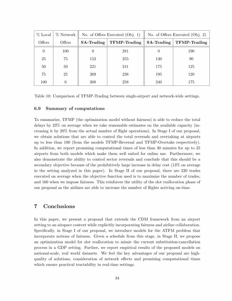
Comparison of TFMP-Trading between single-airport and network-wide settings

In this section, we contrast the performance of TFMP-Trading between single-airport andnetwork-wide settings. It is evident that in the network version, there is a tradeoff betweenthe flexibility of trading slots at different airports versus the added constraint of satisfying allnetwork connectivities. In contrast, in a single-airport setting, there is the advantage of nothaving to satisfy the network connectivity requirements at the expense of losing on tradesacross different airports. So, to compare the two settings, we divide the set of generatedoffers between local and network offers as defined below.

Definition 6.1. An offer (fd, td′ ; fu, tu′) ∈ O is

• a local offer if both the flights involved have the same destination airport, i.e., destfd=

destfu .

• a network offer if the destination airports of the two flights are distinct, i.e., destfd6=

destfu .

Hence, the single-airport model will not have any executed trades that correspond to thenetwork offers. Our overall goal is to demonstrate the utility of TFMP-Trading in executingtrades across offers containing distinct airports. Table 10 reports the results from the twoversions under the two objectives described in Section 4.1. The number reported underTFMP-Trading is the number of offers executed from the network model proposed in thispaper, whereas, SA-Trading (SA stands for single-airport) reports the results obtained fromTFMP-Trading after removing all the network satisfiability constraints and only taking into

32

account the local offers. The numbers reported highlight the tradeoffs inherent in ignoring thenetwork effects vis-a-vis trading slots at different airports. As the percentage of local offersincreases, SA-Trading outperforms TFMP-Trading emphasizing that network connectivitiesare indeed relevant, whereas, for higher fraction of network offers, TFMP-Trading performsbetter reinforcing the utility of network offers. Finally, the number of trades executed withObjective 2 (when fairness is included) are less than 1 Objective which is along expectedlines and demonstrate the flexibility of choosing alternative objective functions.

Objective 1 Objective 2

Day Objective Offers Sol. Time Objective Offers Sol. Time

Cost Executed (in sec.) Cost Executed (in sec.)

14 Jul’04 283 283 13 0 190 29

4 Aug’04 256 256 14 0 180 31

13 May’05 150 150 5 0 140 19

16 Jul’05 278 278 11 0 215 27

27 Jul’05 194 194 9 0 140 22

27 Jul’06 153 153 6 0 90 16

Table 9: Computational performance of TFMP-Trading.PSfrag replacements

Day

No. of executed trades

Airline 1

Airline 2

Airline 3

Airline 4

Airline 5

PSfrag replacements

Day

No. of executed trades

Airline 1

Airline 2

Airline 3

Airline 4

Airline 5

Figure 8: Distribution of number of executed trades across airlines from TFMP-Trading.

Left: (Objective 1 ); Right: (Objective 2 )

33

% Local % Network No. of Offers Executed (Obj. 1) No. of Offers Executed (Obj. 2)

Offers Offers SA-Trading TFMP-Trading SA-Trading TFMP-Trading

0 100 0 281 0 190

25 75 152 255 130 90

50 50 221 241 175 125

75 25 269 238 195 120

100 0 308 258 240 175

Table 10: Comparison of TFMP-Trading between single-airport and network-wide settings.

6.9 Summary of computations

To summarize, TFMP (the optimization model without fairness) is able to reduce the totaldelays by 23% on average when we take reasonable estimates on the available capacity (in-creasing it by 20% from the actual number of flight operations). In Stage I of our proposal,we obtain solutions that are able to control the total reversals and overtaking at airportsup to less than 100 (from the models TFMP-Reversal and TFMP-Overtake respectively).In addition, we report promising computational times of less than 30 minutes for up to 25airports from both models which make them well suited for online use. Furthermore, wealso demonstrate the ability to control sector reversals and conclude that this should be asecondary objective because of the prohibitively large increase in delay cost (13% on averagein the setting analyzed in this paper). In Stage II of our proposal, there are 220 tradesexecuted on average when the objective function used is to maximize the number of trades,and 160 when we impose fairness. This reinforces the utility of the slot reallocation phase ofour proposal as the airlines are able to increase the number of flights arriving on-time.

7 Conclusions

In this paper, we present a proposal that extends the CDM framework from an airportsetting to an airspace context while explicitly incorporating fairness and airline collaboration.Specifically, in Stage I of our proposal, we introduce models for the ATFM problem thatincorporate notions of fairness. Given a schedule from this stage, in Stage II, we proposean optimization model for slot reallocation to mimic the current substitution-cancellationprocess in a GDP setting. Further, we report empirical results of the proposed models onnational-scale, real world datasets. We feel the key advantages of our proposal are high-quality of solutions, consideration of network effects and promising computational timeswhich ensure practical tractability in real-time settings.

34

Acknowledgement

This research has been funded by the NSF Grant EFRI-0735905. We thank Bill Moser andMark Weber of Lincoln Labs for providing us with the data.

Appendix

Strength of TFMP-Reversal:Let us denote the polyhedron induced by the the additional set of constraints to model areversal for each element (f, f ′) ∈ Rj as PReversal(f, f ′, j).

Proposition 1. The polyhedron PReversal(f, f ′, j) is integral.

Proof. PReversal(f, f ′, j) can be written as follows:

PReversal(f, f ′, j) ={x = (wfj,t, sf,f ′,j)| 0 ≤ wfj,t ≤ 1, 0 ≤ sf,f ′,j ≤ 1,

wf′

j,t − wfj,t − sf,f ′,j ≤ 0, t ∈ T reversal

f,f ′,j ,

wfj,t − wf ′

j,t + sf,f ′,j ≤ 1, t ∈ T reversalf,f ′,j .

}We make use of the following two facts from discrete optimization [8]:

Fact 1. Let A be an integral matrix. A is totally unimodular if and only if

{x| a ≤ Ax ≤ b, l ≤ x ≤ u} is integral, for all integral vectors a, b, l, u.

Fact 2. A matrix A is totally unimodular if and only if each collection Q of rows of A can

be partitioned into two parts so that the sum of the rows in one part minus the sum of the

rows in the other part is a vector with entries only 0, +1 and -1.

Consider the following polyhedron P and let A be the matrix such that P = {x|Ax ≤ b}:

P ={x = (wfj,t, sf,f ′,j)|

wf′

j,t − wfj,t − sf,f ′,j ≤ 0, t ∈ T reversal

f,f ′,j ,

wfj,t − wf ′

j,t + sf,f ′,j ≤ 1, t ∈ T reversalf,f ′,j .

}

35

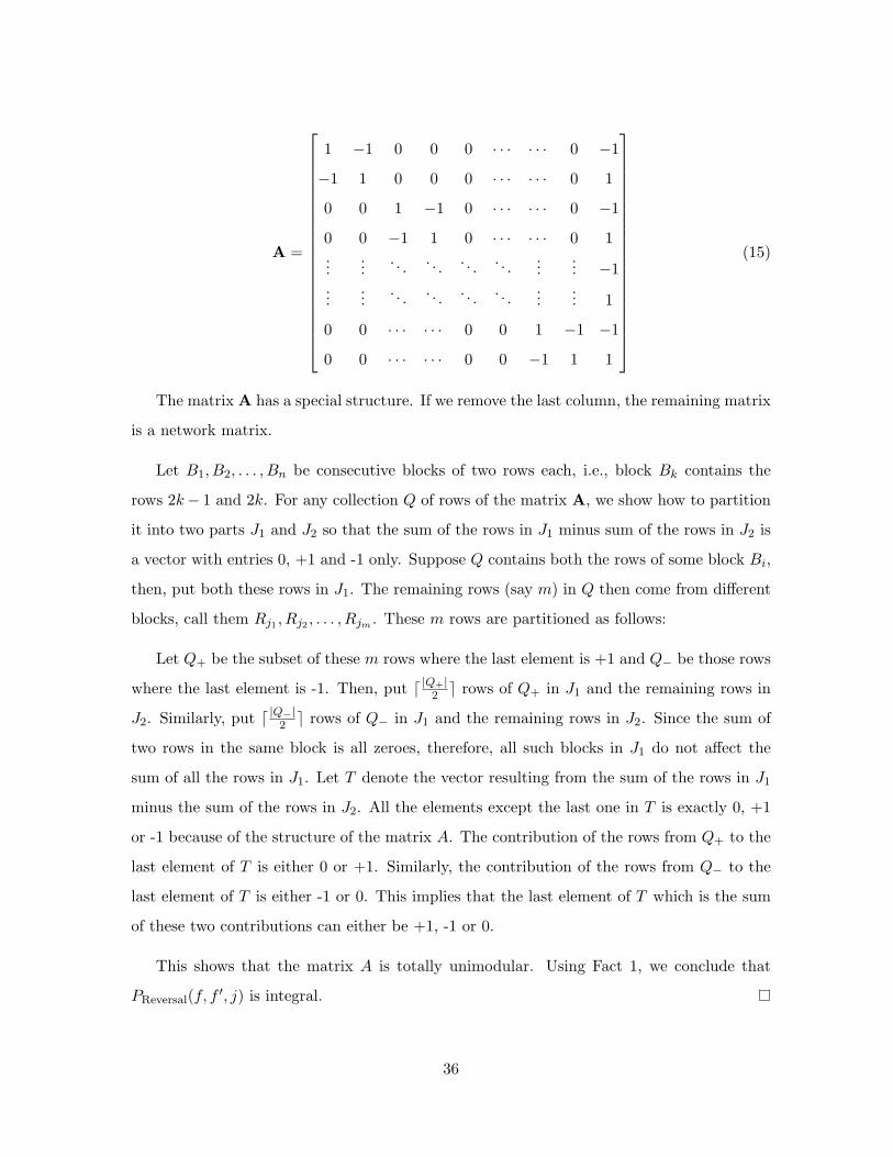
A =

1 −1 0 0 0 · · · · · · 0 −1

−1 1 0 0 0 · · · · · · 0 1

0 0 1 −1 0 · · · · · · 0 −1

0 0 −1 1 0 · · · · · · 0 1...

.... . . . . . . . . . . .

...... −1

......

. . . . . . . . . . . ....

... 1

0 0 · · · · · · 0 0 1 −1 −1

0 0 · · · · · · 0 0 −1 1 1

(15)

The matrix A has a special structure. If we remove the last column, the remaining matrix

is a network matrix.

Let B1, B2, . . . , Bn be consecutive blocks of two rows each, i.e., block Bk contains the

rows 2k− 1 and 2k. For any collection Q of rows of the matrix A, we show how to partition

it into two parts J1 and J2 so that the sum of the rows in J1 minus sum of the rows in J2 is

a vector with entries 0, +1 and -1 only. Suppose Q contains both the rows of some block Bi,

then, put both these rows in J1. The remaining rows (say m) in Q then come from different

blocks, call them Rj1 , Rj2 , . . . , Rjm . These m rows are partitioned as follows:

Let Q+ be the subset of these m rows where the last element is +1 and Q− be those rows

where the last element is -1. Then, put d |Q+|2 e rows of Q+ in J1 and the remaining rows in

J2. Similarly, put d |Q−|2 e rows of Q− in J1 and the remaining rows in J2. Since the sum of

two rows in the same block is all zeroes, therefore, all such blocks in J1 do not affect the

sum of all the rows in J1. Let T denote the vector resulting from the sum of the rows in J1

minus the sum of the rows in J2. All the elements except the last one in T is exactly 0, +1

or -1 because of the structure of the matrix A. The contribution of the rows from Q+ to the

last element of T is either 0 or +1. Similarly, the contribution of the rows from Q− to the

last element of T is either -1 or 0. This implies that the last element of T which is the sum

of these two contributions can either be +1, -1 or 0.

This shows that the matrix A is totally unimodular. Using Fact 1, we conclude that

PReversal(f, f ′, j) is integral.

36

References

[1] Air Transport Association of America Inc., 2008.http://www.airlines.org/economics/cost+of+delays

[2] Ball M., Chen C-Y., Hoffman R., and Vossen T. Colloborative decision making in airtraffic management: Current and future research directions. In Proceedings of ATM’99,Workshop on Advanced Technologies and Their Impact on Air Traffic Management inthe 21st Century. 1999.

[3] Barnhart C., Bertsimas D., Caramanis C., Fearing D. (2009). Equitable and EfficientCoordination of Traffic Flow Management Programs. Submitted to Transportation Sci-ence.

[4] Bertsimas D., Odoni A.R. (1997) A critical survey of optimization models for tacticaland strategic aspects of air traffic flow management. Technical report, NASA.

[5] Bertsimas D., Stock S. (1998) The Air Traffic Management Problem with Enroute Ca-pacities. Operations Research 46, 406-422.

[6] Bertsimas D., Stock S. (2000). The Traffic Flow Management Rerouting Problem inAir Traffic Control: A Dynamic Network Flow Approach, Transportation Science 34,239-255.

[7] Bertsimas D., Lulli G., Odoni A.R. (2008). The Air Traffic Flow Management Problem:An Integer Optimization Approach. IPCO 2008.

[8] Bertsimas D., Weismantel R. (2005). Optimization Over Integers. Dynamic Ideas.

[9] Helme M. (1992). Reducing air traffic delay in a space-time network, IEEE InternationalConference on Systems, Man and Cybernetics 1, 236-242.

[10] Hoffman R., Mukherjee A. and Vossen T. (2007). Air Traffic Flow Management. WorkingPaper.

[11] Lindsay K., Boyd E., Burlingame R. (1993). Traffic flow management modeling with thetime assignment model. Air Traffic Control Quarterly 1, (3), 255-276.

[12] Odoni A.R. (1987). The Flow Management Problem in Air Traffic Control, in FlowControl of Congested Networks, A.R. Odoni, L. Bianco and G. Szego eds., 269-288,Springer-Verlag, Berlin.

[13] Richetta O. and Odoni A.R. (1993). Solving Optimally the Static Ground-Holding PolicyProblem in Air Traffic Control. Transportation Science 27, 228-238.

[14] Richetta O. and Odoni A.R. (1994). Dynamic Solution to the Ground-Holding PolicyProblem in Air Traffic Control. Trans. Res. 28a, 167-185.

[15] Terrab M. and Odoni A.R. (1993). Strategic Flow Control on an Air Traffic Network.Operations Research 41, 138-152.

[16] Terrab M. and Paulose S. (1993). Dynamic Strategic and Tactical Air Traffic FlowControl. RPI Technical Report.

[17] U.S. Dept. of Transportation, Bureau of Transportation Statistics (2008). Airline On-Time Statistics. http://www.transtats.bts.gov/HomeDrillChart.asp

[18] Vossen T., Ball M. Slot Trading Opportunities in Collaborative Ground Delay Programs.Transportation Science. 2006.

37

[19] Vossen T., Ball M. Optimization and Mediated Bartering Models for Ground DelayPrograms. Naval Research Logistics. 2006.

[20] Vranas P.B., Bertsimas D., Odoni A.R. (1994). The Multi-Airport Ground HoldingProblem in Air Traffic Control. Operations Research, 42, 249–261.

[21] Wambsganss M. Collaborative decision making through dynamic information transfer.Air Traffic Control Quarterly, 4:107-123, 1996.

38